DigiCorr III

Leak Noise Water Correlator

User’s Guide

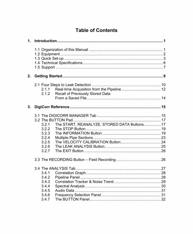
Table of Contents 1. Introduction.................................................................................................... 1 1.1 Organization of this Manual ...................................................................... 1 1.2 Equipment ................................................................................................. 2 1.3 Quick Set-up ............................................................................................. 3 1.4 Technical Specifications............................................................................ 6 1.5 Support ..................................................................................................... 7 2. Getting Started............................................................................................... 9 2.1 Four Steps to Leak Detection ................................................................. 10 2.1.1 Real-time Acquisition from the Pipeline ..................................... 12 2.1.2 Recall of Previously Stored Data From a Saved File...................................................................... 14 3. DigiCorr Reference...................................................................................... 15 3.1 The DIGICORR MANAGER Tab ............................................................ 15 3.2 The BUTTON Pad................................................................................... 17 3.2.1 The START, REANALYZE, STORED DATA Buttons................ 17 3.2.2 The STOP Button....................................................................... 19 3.2.3 The INFORMATION Button ....................................................... 19 3.2.4 Multiple Pipe Sections................................................................ 23 3.2.5 The VELOCITY CALIBRATION Button...................................... 24 3.2.6 The LEAK ANALYSIS Button..................................................... 25 3.2.7 The EXIT Button......................................................................... 26 3.3 The RECORDING Button – Field Recording .......................................... 26 3.4 The ANALYSIS Tab ................................................................................ 27 3.4.1 Correlation Graph....................................................................... 28 3.4.2 Pipeline Panel ............................................................................ 28 3.4.3 Correlation Tracker & Noise Trend ............................................ 29 3.4.4 Spectral Analysis........................................................................ 30 3.4.5 Audio Data ................................................................................. 31 3.4.6 Frequency Selection Panel ........................................................ 31 3.4.7 The BUTTON Panel ...................................................................32

4. Custom Installation ..................................................................................... 33 4.1 Display Setup .......................................................................................... 34 4.2 Serial Port Setup ..................................................................................... 35 4.3 Minimum Hardware Requirements ......................................................... 35 5. Hardware Deployment................................................................................. 37 5.1 Five Steps to Hardware Deployment ...................................................... 37 6. Field Experience .......................................................................................... 41 6.1 Accelerometer Placement....................................................................... 41 6.2 Inter-Sensor Distance ............................................................................. 42 6.3 Sound Velocity ........................................................................................ 43 6.4 Filter Settings .......................................................................................... 43 6.5 Adverse Weather Conditions .................................................................. 43 6.6 Computer Use ......................................................................................... 44 6.7 Correlator-Only Leak Surveys................................................................. 44 7. Tutorial ................................................................................................... 45 7.1 Surveying for Water Leaks Using the DigiCorr ....................................... 45 7.1.1 Planning & Setting Up the Survey.............................................. 45 7.2 Exploring the Advanced Features of the DigiCorr to Pinpoint Difficult-To-Find Leaks............................................ 48 7.2.1 Multiple Leaks Identified in One Correlation Study.................... 49 7.2.2 Frequency-Dependent Results in Correlation............................ 50 8. DigiCorr Pro ................................................................................................... 55 8.1 Digital Mapping Module........................................................................... 55 8.2 HydroData Management Module ............................................................ 56

1

1 Introduction

The DigiCorr analyzes leaks using a state-of-the-art computerized instrument running under the Windows Operating System. By combining the speed and ease of use of a visual environment with the power and flexibility of the world’s gold standard for acoustic leak detection, the DigiCorr offers the following features:

Computerized, fully-automated Field Sensor Units (FSUs)

CD quality leak sounds transmitted digitally from the FSUs to the base unit

Easy to use Windows-based software

Fully upgradeable through software from Flow Metrix Research

Simple 1-action analysis of leaks

1.1 Organization of this manual

Chapter 1 “Introduction” lists all the components of the equipment, technical specifications, and essential support information.

Chapter 2 “Getting Started” covers setting up the equipment in the field, finding leaks and will show you how to take full advantage of all of the DigiCorr’s features.

Chapter 3 “DigiCorr Reference” is a reference section explaining all of the options that the DigiCorr has to offer.

Chapter 4 “Custom Installation” explains how to install the software package on your own Windows-based computer system.

Chapter 5 “Hardware Deployment” explains the optimal hardware deployment.

Chapter 6 “Field Experience” includes actual field experience, which will help to optimize the performance of the system.

Chapter 7 “Tutorial” walks the DigiCorr user through some routine and

non-routine readings.

1.2 Equipment The DigiCorr comes with the following equipment either as part of the standard package or as options:

2

Ruggedized, all-weather computer Rugged, waterproof carrying cases

Weatherproof, computerized Field Sensor Units with digital LeDetection Processing and Digital DataStream transmission

Base Station Radio 2-way transceiver AC01 high performance accelerometers, fully immersible (150

pull force), and magnet (50 lb [23 kg] pull force) Leak detection hydrophones (optional) Headphones (not shown)

ak

lb [70 kg]

1.3 Quick Set-up Step One - Turn on the computer

NOTE: If you intend to work with the program for a long period of time, we recommend the computer be connected to an electrical source such as an auto power inverter, if working in the field, or an electrical outlet, if working in the office.

Step Two – Attach serial cable to the computer (COM1) and then to the Digital Transceiver. (Make sure the connections are tight.)

3

Step Three – Plug the USB power cord into the power socket on the Digital Transceiver and then plug into the USB socket on the computer. (This cord powers the Digital Transceiver - the LED on the Digital Transceiver should be solid green.)

Step Four – Attach an antenna to the antenna socket on the Digital Transceiver. (If operating from a vehicle, use the magnetic roof mounted antenna. If in the office or away from the vehicle attach a whiplash antenna.)

4

Step Five - Attach an Accelerometer to each Field Sensor Unit (FSU).

(It is important to inspect each cable prior to use to make sure they have not been damaged. Any cut or tear on the outer jacket may indicate internal damage and this could adversely affect any

recording. Send any damaged accelerometer assembly to Flow Metrix for repair immediately.)

Step Six – Place each accelerometer on an access point to the pipe - hydrant, valve, etc.

5

Step Seven – Turn on each FSU.

The Field Sensor Units (FSUs) are computerized and fully automated. To deploy the units in the field follow these steps:

1. Connect the sensor cable to the black chrome connector on the top

of the FSU.

2. Connect the antenna to the TNC antenna socket on the top of the FSU.

3. Press the power switch on the top of the FSU. In the “On” position,

the power light will go through the following “power up” flash sequence: red - yellow – green/green. If the FSU is not linked to the transceiver it will then turn red. It will turn green when the FSU is linked to the base transceiver.

The blue LED will flash once indicating it the unit is prepared to transmit

data. The blue LED will flash continuously when actively transmitting data.

6

1.4 Technical Specifications Field Sensor Units (FSU) Pipeline Sensors • Accelerometers: Sensitivity = 12V/g; Noise < 0.05:g/√Hz; Bandwidth = 1 – 4,000 Hz • Hydrophones and microphones are available for in-flow and other measurements FSU Radio Transceivers • Noise-free digital transmission • ISM/LAN 2.4 GHz spread spectrum, license-free worldwide, FCC approved • Range from 3300 to 10,000 feet [1 to 3 kilometers] (line-of-sight) • Two-way communication with base station radio transceiver Power Supply • Intelligent power management • Up to 50 hours battery life, rechargeable • Common re-charger for FSUs and base station radio transceiver; AC outlet or Data Acquisition • Intelligent automatic gain = 10 – 80,000 with remote manual adjustment at base station • 16-bit data acquisition, 92 dB dynamic range, 0.01% linearity, sampling rate = 5 kHz Physical Characteristics • Size and weight: cylindrical, diameter = 6 inches, height = 9 inches, 6 pounds • Rugged, metal case Base Station Radio Transceiver Power Supply • Powered through USB port of computer with supplied power cord. May also be

powered through AC outlet or standard auto DC Physical Characteristics • Size and weight: 5 x 3.25 x 1 inches, 1 pound • Rugged, metal, weatherproof enclosure DigiCorr Software Easy to use, MS Windows 95/98/2000/XP ALFATM (Automatic Leak Frequency Analysis) High resolution display of correlation function, on-screen, land-marked location of

detected leaks Correlation range: ± 880 milliseconds 15 types of pipe materials, including multiple sections of different pipe types Automatic sound velocity measurement Manual selection of possible leaks from correlation function Spectral (FFT) analysis capability Digital Filters with full manual frequency band selection available: High-pass: 10 –

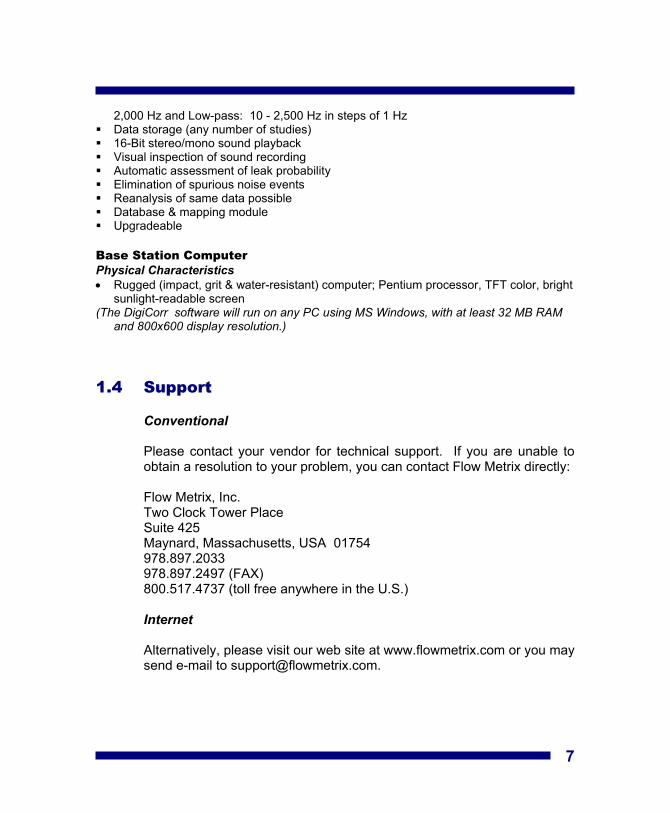
7

2,000 Hz and Low-pass: 10 - 2,500 Hz in steps of 1 Hz Data storage (any number of studies) 16-Bit stereo/mono sound playback Visual inspection of sound recording Automatic assessment of leak probability Elimination of spurious noise events Reanalysis of same data possible Database & mapping module Upgradeable

Base Station Computer Physical Characteristics • Rugged (impact, grit & water-resistant) computer; Pentium processor, TFT color, bright

sunlight-readable screen (The DigiCorr software will run on any PC using MS Windows, with at least 32 MB RAM

and 800x600 display resolution.) 1.4 Support Conventional

Please contact your vendor for technical support. If you are unable to obtain a resolution to your problem, you can contact Flow Metrix directly:

Flow Metrix, Inc. Two Clock Tower Place Suite 425 Maynard, Massachusetts, USA 01754 978.897.2033 978.897.2497 (FAX) 800.517.4737 (toll free anywhere in the U.S.) Internet

Alternatively, please visit our web site at www.flowmetrix.com or you may send e-mail to support@flowmetrix.com.

8

2

Getting Started We suggest you read this short section while working with the DigiCorr. The DigiCorr software may be started from either the Windows desktop or the task bar. The first screen should look like Figure 2.1:

9

Figure 2.1 The Splash Screen

he next screen is the Login Dialog and should look like Figure 2.2: g

nter the information requested

Location are

ng the STORED DATA

usly

The splash screen is displayed for approximately 10 seconds. During this time the DigiCorr attempts to link to the Field Sensor Units (FSUs). If the radio link is successful, the units are placed in low-power consumption mode. If the radio link is unsuccessful, the attempt will be repeated every five minutes automatically.

T Figure 2.2 The Login Dialo Ein the Login Dialog:

The User andsaved with any stored data. The Sensor Type is requiredand is saved with any stored data. Pressibutton bypasses the Login Dialog and permits a previostored data file to be opened.

10

fter you have finished entering the requested information, press OK. The

.1 Four Steps to Leak Detection

tep 1: Enter the Pipeline Information

efore a leak can be

sound velocity are available - see the next sec

To select the pipe material, click on the down arrow to the right of the

To enter the pipe diameter, click in the text box and type a value, e.g.,

ADigiCorr Manager Screen now appears as shown in Figure 3.1 (With Maps) or Figure 3.2 (With Grid) depending upon having had your distribution system maps integrated into the DigiCorr software. 2 S

Bdetected, it is necessary to know the velocity of sound propagation in the pipeline. In almost all cases, this is simply a matter of selecting the Pipeline Material and entering the Pipe Diameter. (Other means of measuring the tion.)

text box. Select a pipe material from the drop down menu of options.

“100.” Then, press ENTER or click elsewhere on the screen. The DigiCorr accepts the value if it is within range and has not been mistyped. The DigiCorr also adds units, i.e., “mm” for millimeters if the system units are metric or “inches” otherwise.

S

11

file.)

tep 2: Place Sensors on Map (Grid) & Enter Distance Between

Click on the Map icon in the Map Panel to

Navigate through the maps using the arrow

Click on the Red FSU image in the Map

A distance will be calculated based on the selected map locations. The

w and Blue Sensors

ter

Blue sensor. These addresses will be saved with the recording.

Sensors

bring a map or the grid into the Map Window. (You can also enter a map name.)

buttons in the Map Panel to find the location of the valves or hydrants where the sensors have been placed. (The Zoom icon will expand the map for easier navigation.)

Window and then click on its location on the map or grid. Then do the same for the Blue FSU. (These locations will be saved with the

distance can be overridden or entereddirectly by clicking in the Sensor Distance text box and typing in the

distance between FSUs.

Step 3: Enter Address for Yello

Click on “Address” next to the Red box on the Pipeline Graphic and enthe address of the Red sensor, such as “V152” for valve number 152, and press Enter. You will then be prompted to enter the address for the

tep 4: Start a Correlation Analysis

Click on the START button and Real-time analysis from the e

Figure 2.4 The Start Recording Dialog

2.1.1 Real-time Acquisition From the Pipeline

The Digital Data Transceiver (DDT) will attempt to link to the FSU radios.

S

pipeline begins with the Digi mpting to link to the Field SensorUnits. The Start Recording Dialog is shown in Figure 2.4:

Corr att

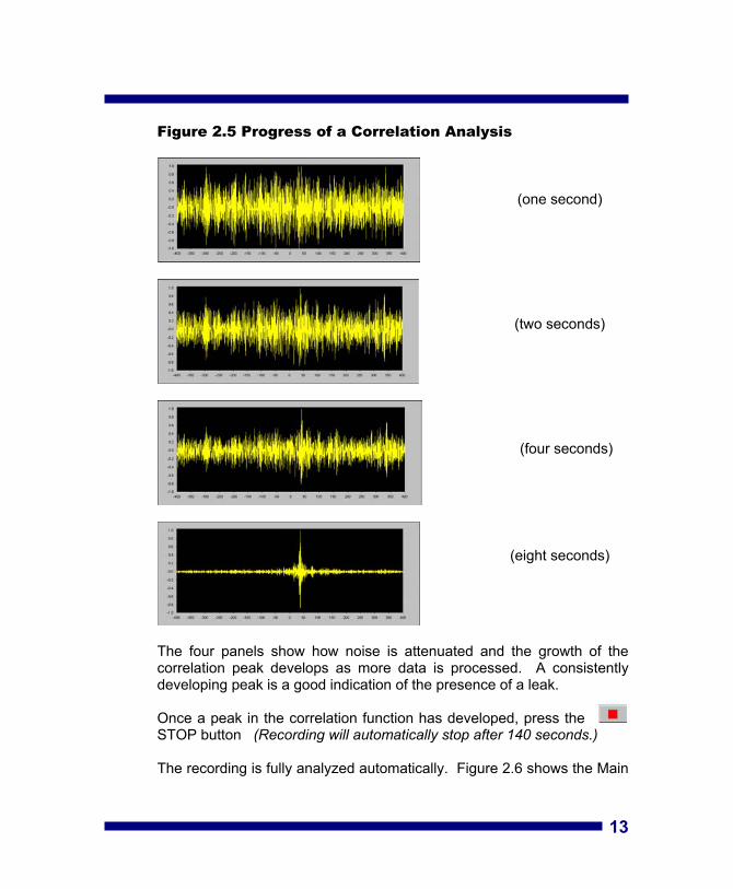
Once the DDT and FSU radios are linked, the correlation process will begin automatically. The progress of a correlation analysis is shown after 1, 2, 4 and 8 seconds (top to bottom) in the four panels in Figure 2.5. The peak that develops in the correlation function indicates a leak. It usually takes between one and thirty seconds (maximally 90 seconds) for a distinct peak to develop.

procedures

NOTE: If you are unable to link to the FSU radios, follow thedescribed in Section 3.1.1.

12

13

.5 Progress of a Correlation Analysis Figure 2

(one second)

(eight seconds)

(four seconds)

(two seconds)

The four panels show how noise is attenuated and the growth of the

Once a peak in the correlation function has developed, press the

he recording is fully analyzed automatically. Figure 2.6 shows the Main

correlation peak develops as more data is processed. A consistently developing peak is a good indication of the presence of a leak.

STOP button (Recording will automatically stop after 140 seconds.

)

T

Screen after the automatic detection of the correlation peak. Figure 2.6 The Main Screen After Correlation & Leak

The correlation peak

f the

here is an actual leak present. The distance betwee h

.1.2 Recall of Previously Stored Data From A Saved File

The example in 2.4.1 shows a real-time correlation analysis from data

Detection

shows the difference in time of arrival of the leaksound between the red sensor and the blue sensor. The position oleak is marked on thepipeline graphic by a vertical red bar. The thickness of the bar (1,to 4pixels) is proportional to the likelihood that t

n the leak position and eacof the sensors is shown above the pipeline. 2

recorded by the FSUs on the pipeline. Alternatively, correlation analyses may be made by clicking on the STORED DATA button. The Stored Data Dialog appears as shown in Figure 2.7:

Figure 2.7 The Stored Data Dialog default, the Stored Data

y

ins

ByDialog opens in the director“c:\data”. Select a data file byhighlighting the file name and click on the OK button. The correlation analysis now begautomatically and proceeds as shown above in Figures 2.5 and2.6.

14

3 DigiCorr Reference

This reference section is organized around the following: The DigiCorr Manager Tab The Recording Screen The Analysis Tab

3.1 The DigiCorr Manager Tab The DigiCorr Manager Screen appears as shown in Figure 3.1 (With Maps) or Figure 3.2 (With Grid) depending upon having had your distribution system maps integrated into the DigiCorr software.

15

Figure 3.1 The DigiCorr Manager Screen (With Maps)

Figure 3.2 The DigiCorr Manager Screen (With Grid)

16

A E

B

C

D The elements of the DigiCorr Manager Screen are: A. Correlation Window - Displays the cross-correlation function in

real-time as data is processed. B. Pipeline Graphic - Schematically represents the position of the

ed and blue Field Sensor Units (FSUs) and the position of the leak(s) if any leak is detected.

C. Button Pad - Used to control the program: the function of each button is defined in Section 3 of this manual.

D. Frequency Selection and Pipeline Panels - Shows the status of ALFA (Automatic Leak Frequency Analysis), the manual digital filter settings, the settings of the electronic gain of the FSUs, and the critical pipeline information needed to calculate the velocity of sound propagation in the pipe. ALFA is selected by default (button outlined in blue). Two other buttons are available: Advanced and Save.

E. Map/Grid Section - Allows sensors to be placed on the map (if integrated) or grid indicating the approximate placement of the sensors in the field.

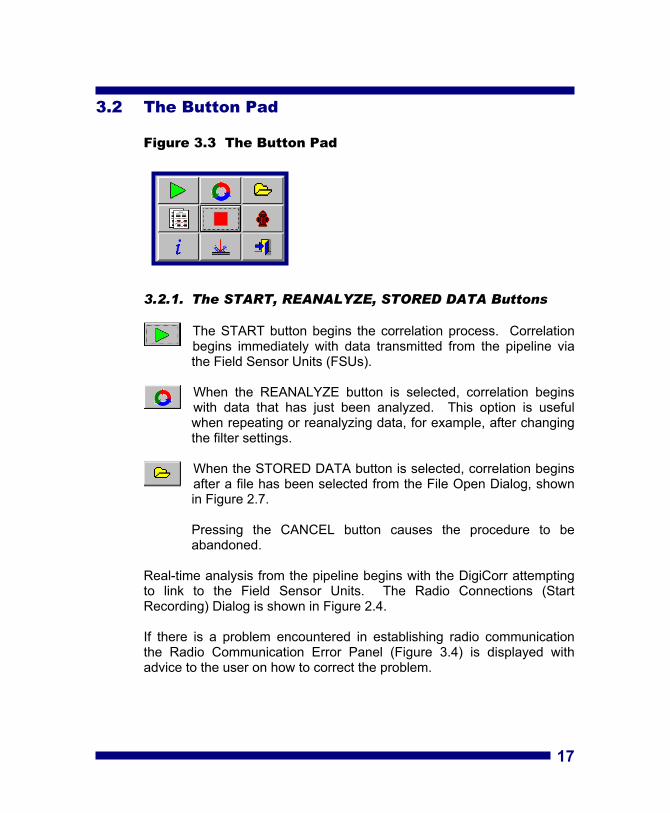
3.2 The Button Pad

Figure 3.3 The Button Pad

17

3.2.1. The START, REANALYZE, STORED DATA Buttons

The START button begins the correlation process. Correlation begins immediately with data transmitted from the pipeline via the Field Sensor Units (FSUs). When the REANALYZE button is selected, correlation begins with data that has just been analyzed. This option is useful when repeating or reanalyzing data, for example, after changing the filter settings. When the STORED DATA button is selected, correlation begins after a file has been selected from the File Open Dialog, shown in Figure 2.7.

Pressing the CANCEL button causes the procedure to be abandoned.

Real-time analysis from the pipeline begins with the DigiCorr attempting to link to the Field Sensor Units. The Radio Connections (Start Recording) Dialog is shown in Figure 2.4.

If there is a problem encountered in establishing radio communication the Radio Communication Error Panel (Figure 3.4) is displayed with advice to the user on how to correct the problem.

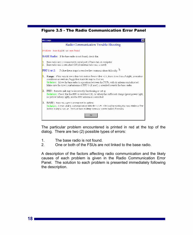
Figure 3.5 - The Radio Communication Error Panel

The particular problem encountered is printed in red at the top of the dialog. There are two (2) possible types of errors:

1. The base radio is not found. 2. One or both of the FSUs are not linked to the base radio.

A description of the factors affecting radio communication and the likely causes of each problem is given in the Radio Communication Error Panel. The solution to each problem is presented immediately following the description.

18

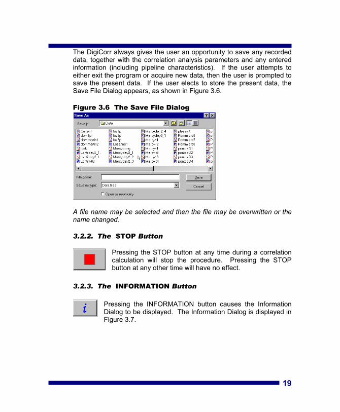
The DigiCorr always gives the user an opportunity to save any recorded data, together with the correlation analysis parameters and any entered information (including pipeline characteristics). If the user attempts to either exit the program or acquire new data, then the user is prompted to save the present data. If the user elects to store the present data, the Save File Dialog appears, as shown in Figure 3.6.

Figure 3.6 The Save File Dialog

A file name may be selected and then the file may be overwritten or the name changed. 3.2.2. The STOP Button

Pressing the STOP button at any time during a correlation calculation will stop the procedure. Pressing the STOP button at any other time will have no effect.

3.2.3. The INFORMATION Button

Pressing the INFORMATION button causes the Information

Dialog to be displayed. The Information Dialog is displayed in Figure 3.7.

19

F

20

file.

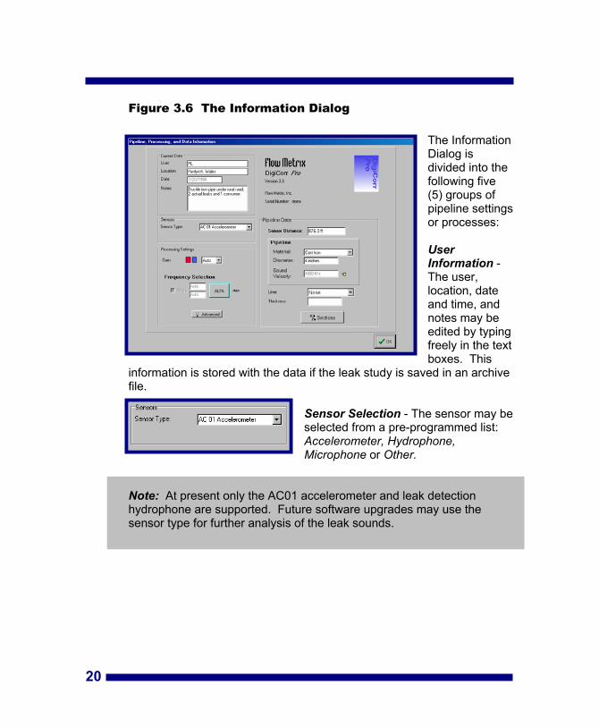
igure 3.6 The Information Dialog

divided into the ing five

ttings

boxes. This information is stored with the data if the leak study is saved in an archive

or may be

ogrammed list: Accelerometer, Hydrophone, Microphone or Other.

leak detection hydrophone are supported. Future software upgrades may use the sensor type for further analysis of the leak sounds.

The Information Dialog is

follow(5) groups of pipeline seor processes:

User Information - The user, location, dateand time, and notes may be edited by typingfreely in the text

Sensor Selection - The sensselected from a pre-pr

Note: At present only the AC01 accelerometer and

21

n

s

Gain value (initial volume is Gain = 40).

right side of the Gain list box and select a gain between 20 and 80,000.

isabled entirely by clicking the check box to the left of the label “Filters”.

ion 3.4.2) have been altered, the bulb is illuminated as shown to the left.

ber

e of can be

changed by the user.)

Gain/Filter Settings - Automatic Gaiis selected by default (“Auto”) and ioptimal for correlation in almost all situations. The headphone audio level at the FSUs is adjusted by selecting a

With Automatic Gain, the FSUs will scale the data for the best resolution. In the event that manual gain settings are needed, click on the arrow at the

The ALFA setting is active by default. With ALFA the DigiCorr software will perform optimal filtering automatically to detect any correlations present. However, digital filter settings may be changed manually by clicking the ALFA button off and entering values directly in the Filter text boxes. The range of values is 1 to 2,450 Hz, in steps of 1 Hz. Filters may be d

Advanced Dialog - The Advanced Processing Options Dialog can be accessed by pressing the ADVANCED button. In the Information Dialog of

Figure 3.6, the ADVANCED button’s bulb is off, indicating that the settings are at their default value. Once the advanced settings (see Sect

Product and Serial NumInformation - The serial number is unique to your software. Please note that each FSU has its own serial number, distinct from that of the DigiCorr software. (Nonthe items in this dialog

22

sults. Pipe pressure is stored with data saved to archive

tion

in

in

ysis:

the se

pipeline is computed

automatically from tables in the DigiCorr software.

tered directly, then the pipeline material and diameter are ot needed.

nt - see the description of the CALIBRATION button in Section 3.2.5.)

files.

ns, invokes the Multiple Pipe Sections Dialog as shown in Figure 3.7.

Pipeline Data - This panel in the InformaDialog allows more detailed information to beentered than in the MaScreen. The itemsbold are generally needed to perform automatic leak analDistance between sensors; Material of the pipeline; Diameter of pipeline. Once thevalues have been entered, the Velocity of Sound Propagation inthe

NOTE: If the Velocity of Sound Propagation in the pipe is known and has been enn Over long distances (typically over one (1) mile between sensors), the sound velocity calculation can be improved by entering the thickness of the pipe, if known. (The Velocity of the Sound Propagation can also be measured using a hydra

NOTE: The pressure of the pipeline can also be entered. Although not used directly by the DigiCorr, it can be useful to know when interpreting correlation re

Pressing the PIPE SECTIONS button, or increasing the number of pipe sectio

3.2.4. Multiple Pipe Sections

different materials or diameters, can be specified in the following ways:

Select Multiple Sections as the pipe material.

ter than one (1) in the Information Dialog.

Multiple sections of pipe, sections with

Select the number of pipe sections to be grea

23

Pressing the CLEAR button resets the dialog, losing all information.

est to the red FSU with e last filled-in section closest to the blue FSU.

Press the MULTIPLE PIPE SECTIONS button.

Figure 3.7 Multiple Sections of Pipe Dialog

ctly.

The user can now enter data for each section, up to a possible total of four (4) pipe sections. The Length, Material, and Diameter are required for each section, or the Sound Velocity may be entered dire

NOTE: The first section is assumed to be closth

24

Mode

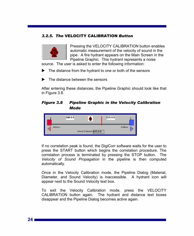
3.2.5. The VE OCITY CALIBRATION Button

the noise

The distance from the hydrant to one or both of the sensors

The distance between the sensors

nces, the Pipeline Graphic should look like that in Figure 3.8.

Figure 3.8 e Graphic in the Velocity Calibration

ound Propagation in the pipeline is then computed automatically.

sible. A hydrant icon will appear next to the Sound Velocity text box.

ce text boxes disappear and the Pipeline Dialog becomes active again.

L

Pressing the VELOCITY CALIBRATION button enablesautomatic measurement of the velocity of sound in the pipe. A fire hydrant appears on the Main Screen in Pipeline Graphic. This hydrant represents a

source. The user is asked to enter the following information:

After entering these dista

Pipelin

If no correlation peak is found, the DigiCorr software waits for the user to press the START button which begins the correlation procedure. The correlation process is terminated by pressing the STOP button. The Velocity of S

Once in the Velocity Calibration mode, the Pipeline Dialog (Material, Diameter, and Sound Velocity) is inacces

To exit the Velocity Calibration mode, press the VELOCITY CALIBRATION button again. The hydrant and distan

When the velocity of sound has been calculated, it is stored until a new velocity of sound is computed by:

1. Changing the pipeline material and diameter; or

25

n the pipeline can be

determined in one of the three following ways:

r extra accuracy) Thickness (found in the Information

Dialog).

noise source (see VELOCITY CALIBRATION button reference section).

Velocity text box, either on the ain Screen or the Information Dialog.

2. Directly entering a new value in the Sound Velocity text box.

the calibrated value, press the VELOCITY CALIBRATION button

3.2.6. The EAK ANALYSIS Button

of the leak from each sensor using the following items of information:

The distance between sensors

city of sound propagation in the pipeline

r both of these items is missing, the DigiCorr will prompt for data entry.

If a new velocity of sound value has been computed and you wish to retrieveagain. NOTE: The velocity of the sound propagation i

Calculation from formulae using Pipe Material, Diameter, and

(optionally fo

Calibration from an open hydrant or other

Direct data entry in the Sound

M

L When the LEAK ANALYSIS button is pressed, the DigiCorr searches for peaks in the current correlation waveform. Strong peaks represent the difference in time of arrival of

the leak sound at the two sensors. The timing of the peaks is translated to a distance

The velo If one o

26

3.2.7. The EXIT Button

d, the base station computer closes the DigiCorr software.

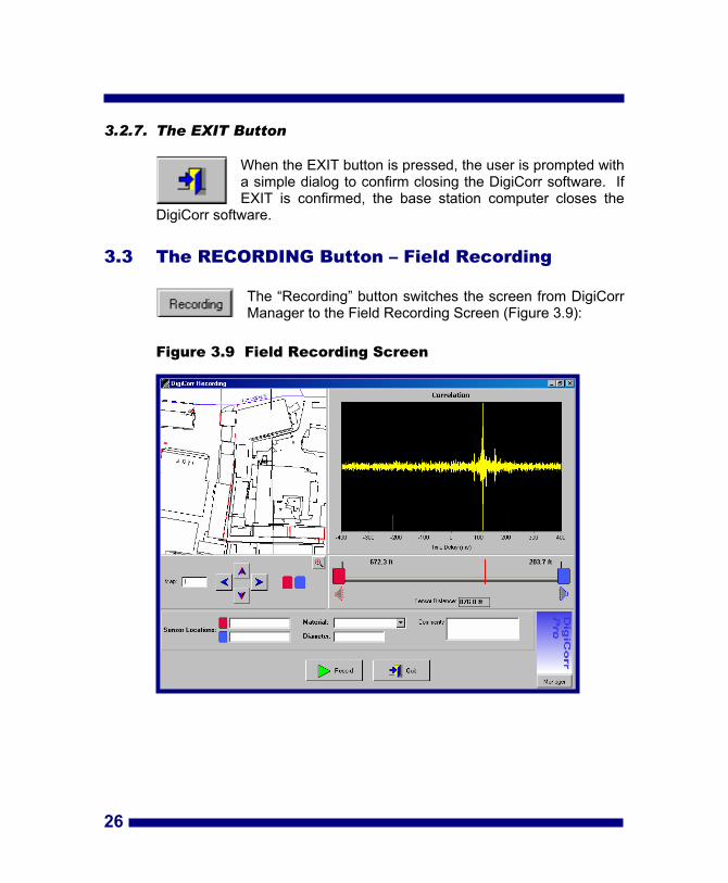
3.3 The RECORDING Button – Field Recording

iCorr Manager to the Field Recording Screen (Figure 3.9):

Figure 3.9 Field Recording Screen

When the EXIT button is pressed, the user is prompted with a simple dialog to confirm closing the DigiCorr software. If EXIT is confirme

The “Recording” button switches the screen from Dig

27

The recording process is simple:

Step 1: heir position on the map. Select the pipe material and diameter.

Step 2:

atically. (The recording information is added to the database.)

Any missing information is prompted for at the end of the recording.

e MANAGER button to return to the Manager Screen.

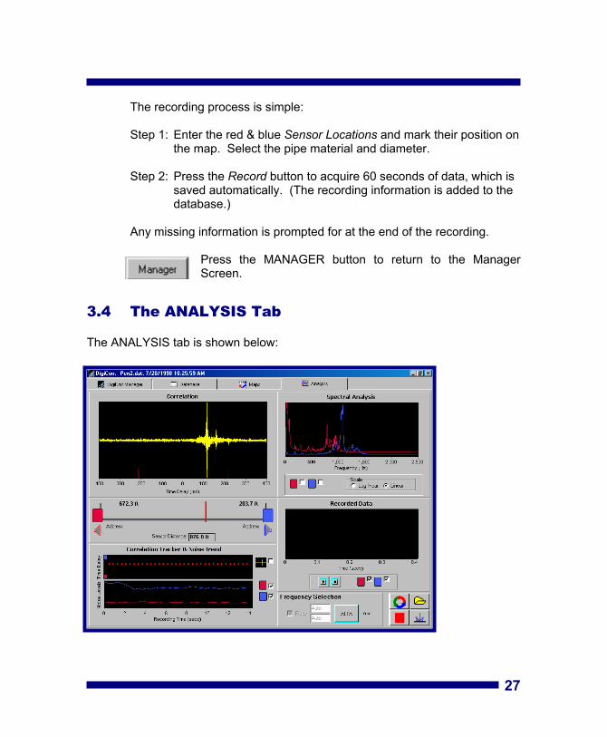
3.4 The ANALYSIS Tab

The ANALYSIS tab is shown below:

Enter the red & blue Sensor Locations and mark t

Press the Record button to acquire 60 seconds of data, which is saved autom

Press th

28

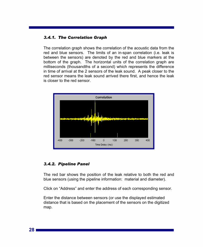
3.4.1. The Correlation Graph

sound arrived there first, and hence the leak is closer to the red sensor.

3.4.2. ipeline Panel

nd blue se ors (using the pipeline information: material and diameter).

Click on “Address” and enter the address of each corresponding sensor.

that is based on the placement of the sensors on the digitized map.

The correlation graph shows the correlation of the acoustic data from the red and blue sensors. The limits of an in-span correlation (i.e. leak is between the sensors) are denoted by the red and blue markers at the bottom of the graph. The horizontal units of the correlation graph are milliseconds (thousandths of a second) which represents the difference in time of arrival at the 2 sensors of the leak sound. A peak closer to the red sensor means the leak

P

The red bar shows the position of the leak relative to both the red ans

Enter the distance between sensors (or use the displayed estimated distance

Click the Smart Listen icon next to ea

29

ch sensor to hear the quietest 8 seconds of the recording, avoiding any traffic or other temporary disturbances that might be present.

3.4.3.

ch ½ second during the recording. The lower half of the graph is towards the red sensor, the top half towards the blue.

Correlation Tracker & Noise Trend

The Correlation Tracker shows the location of the strongest correlation peak at ea

Silver dot - a peak that is not recognized Red dot - a peak with modest probability of a leak Red open circle - a peak with moderate probability of a leak Solid red circle - a peak with high probability of a leak

The Noise Trend shows the noise levels at the red and blue ensors at the same times.

s

In the example above, there is some extraneous noise initiallythe blue sensor (a passing vehicle or sudden usage, for example). The correlation takes 4 seconds to develop into a strong peak, which does not vary in location. Noise at the red sensor after

30

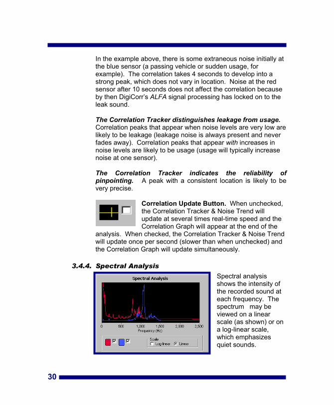
3.4.4. Spectral Analysis

at

10 seconds does not affect the correlation because y then DigiCorr’s ALFA signal processing has locked on to the

re

on peaks that appear with increases in noise levels are likely to be usage (usage will typically increase

tion Tracker indicates the reliability of pinpointing. A peak with a consistent location is likely to be very precise.

Noise Trend will update once per second (slower than when unchecked) and

te simultaneously.

ity of at

r on scale,

which emph sizes quiet sounds.

bleak sound. The Correlation Tracker distinguishes leakage from usage. Correlation peaks that appear when noise levels are very low alikely to be leakage (leakage noise is always present and never fades away). Correlati

noise at one sensor).

The Correla

Correlation Update Button. When unchecked, the Correlation Tracker & Noise Trend will update at several times real-time speed and the Correlation Graph will appear at the end of the

analysis. When checked, the Correlation Tracker &

the Correlation Graph will upda

Spectral analysis shows the intensthe recorded soundeach frequency. The spectrum may be viewed on a linear scale (as shown) oa log-linear

a

31

The e

eaks (<600 Hz) are more often associated with mains leaks

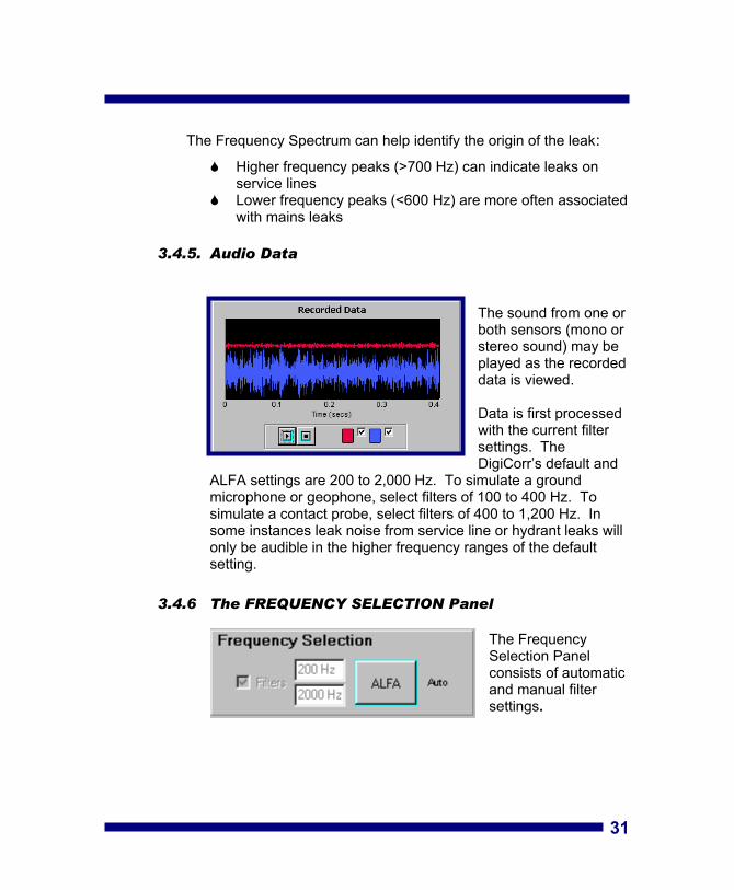
.4.5. Audio Data

corded

d

oise from service line or hydrant leaks will only be audible in the higher frequency ranges of the default

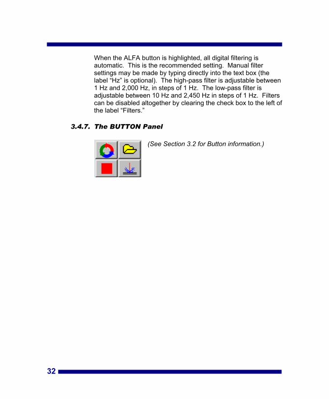
3.4.6 The FREQUENCY SELECTION Pane

automatic and manual filter

ttings.

Fr quency Spectrum can help identify the origin of the leak: Higher frequency peaks (>700 Hz) can indicate leaks on

service lines Lower frequency p

3

The sound from one or both sensors (mono or stereo sound) may be played as the redata is viewed.

Data is first processewith the current filter settings. The DigiCorr’s default and

ALFA settings are 200 to 2,000 Hz. To simulate a ground microphone or geophone, select filters of 100 to 400 Hz. To simulate a contact probe, select filters of 400 to 1,200 Hz. In some instances leak n

setting.

l

The Frequency Selection Panel consists of

se

32

, in steps of 1 Hz. The low-pass filter is adjustable between 10 Hz and 2,450 Hz in steps of 1 Hz. Filters

r by clearing the check box to the left of the label “Filters.”

l

ee Section 3.2 for Button information.)

When the ALFA button is highlighted, all digital filtering is automatic. This is the recommended setting. Manual filter settings may be made by typing directly into the text box (the label “Hz” is optional). The high-pass filter is adjustable between 1 Hz and 2,000 Hz

can be disabled altogethe

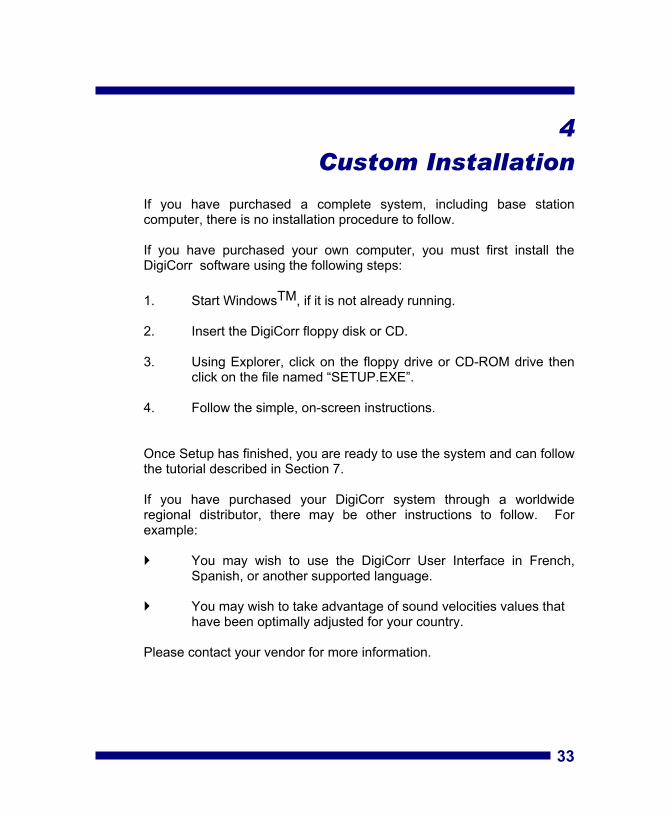
3.4.7. The BUTTON Pane (S

33

4 Custom Installation

ing base station computer, there is no installation procedure to follow.

, you must first install the

DigiCorr software using the following steps:

. Start WindowsTM, if it is not already running.

2. Insert the DigiCorr floppy disk or CD.

3. e or CD-ROM drive then click on the file named “SETUP.EXE”.

4. Follow the simple, on-screen instructions.

ady to use the system and can follow

the tutorial described in Section 7.

istributor, there may be other instructions to follow. For example:

r Interface in French, Spanish, or another supported language.

ities values that have been optimally adjusted for your country.

Please contact your vendor for more information.

If you have purchased a complete system, includ

If you have purchased your own computer

1

Using Explorer, click on the floppy driv

Once Setup has finished, you are re

If you have purchased your DigiCorr system through a worldwide regional d

You may wish to use the DigiCorr Use

You may wish to take advantage of sound veloc

4

34

ensors,

splay

tion:

1. itions, or a large number of

2. the base unit have low batteries (indicated by a yellow power light).

.1 Display Setup

ou select “large font” from the Windows Control Panel Display Option.

f you will be

using the computer to record data from the pipeline sensors.

If you have purchased your own computer, it may be necessary to select a compatible graphics display. The DigiCorr works best at a screen resolution of 800 x 600 pixels. Display resolutions of 640 x 480 and 1024 x 768 are also supported. If standard VGA resolution (640 x 480) is used, then it is recommended that y

Set the color depth (number of colors) to either 16-bit or 256 i

NOTE: If the message “Radio Transmission Interrupted - Please Restart” appears frequently when recording data from the pipeline sthen a problem related to Windows ‘95 interrupt latency is probably occurring. To resolve this problem, set the number of colors in the display to either 16-bit or 256, as needed (using the Windows ‘95 Control Panel DiOption). You may also have to disable Windows power management. Please contact your vendor for a solution if the problem persists. CauThis message may also occur under the following circumstances:

The radio link between the FSUs and the base is periodically lost due to extreme range, highly adverse weather condobstructions such as foliage and buildings. The FSUs or

4.2 Serial Port Setup

If you have purchased your own computer, it is necessary to setup the serial port for real-time data acquisition. To do this, select the System Option in the Windows ‘95 Control Panel. Select the tab labeled HARDWARE and then select PORTS and COM1. The following settings should be made:

Baud Rate: 115200 No. of Data Bits: 8 Parity: None No. of Stop Bits: 1 Flow Control: Hardware 4.3 Minimum Hardware Requirements

The DigiCorr has been designed to run on any computer that meets the following minimum configuration requirements:

Processor: 266 MHz Pentium, or faster Memory: 32 Mbytes RAM or more Hard Disk Space: 120 Mbytes or more Sound card: 16-bit Sound BlasterTM, or compatible Display: At least 640 x 480 standard VGA, active matrix

or daylight readable recommended (800 x 600 preferred)

Serial port: Standard port capable of 115 kbits/second with UART 1655 or better, assigned to COM255 0

Operating System: WindowsTM

NOTE: Every attempt has been made to ensure that the DigiCorr will run without problems on any IBM PC-compatible computer. However, there can be no guarantee that the software will operate flawlessly on any computer not supplied as part of the DigiCorr system.

35

36

37

5 Hardware Deployment

5.1 Five Steps to Hardware Deployment

Step One - Choose Sensor Type

In most cases, accelerometers will be adequate. The accelerometers provide ease and flexibility of deployment.

Consider hydrophones for:

Large diameter pipes (>12”) which may be partially filled with air Plastic pipes Service lines on the consumer side of the meter (wall faucet) Locations with excessive ambient noise (e.g. airports)

Step Two - Choose Points of Deployment

When choosing deployment sites, consider these basic

questions: Where is the leak?

Leaks tend to occur at stress points. Old repairs give clues.

Where will the sound travel?

Sound travels in the water, not the pipe. Sound is attenuated in lateral connections. Sound is proportional to pressure.

38

Select points which likely span the leak site but are as close together as possible.

1. Locate 1st sensor as close to the suspected leak site as

possible 2. Locate 2nd sensor where the leak sound is most likely to

travel: a. the same pipe; b. a lateral line with closest diameter (similar flow &

pressure); or c. physically nearest point (e.g. meter) to leak

Listening may aid in selecting sensor points, however: 1. Sound is attenuated between pipes in proportion to change in

pressure & diameter. 2. Sound levels attenuate at: 0.05 dB/m — cast iron 0.25 dB/m — PVC 3. It is often not possible to hear leaks on plastic pipes at distances

greater than 30 ft

When choosing sensor sites on mains: Hydrophones attach to hydrants (typically 300 - 500 feet spacing) Accelerometers prefer in-line main valves away from a lateral pipe

connection (avoid 4-way) OR pressurized (i.e. water-filled) hydrants (connected to base or on hydrant valve)

39

When choosing sensor sites on service lines:

Hydrophones may be useful on an outside faucet (open) if leak is on the consumer’s side of the meter

Accelerometers can be connected at meters. Fittings are usually

not ferrous (magnetic), therefore sensor must rest on pipe. Use only over short distances (< 200 feet) and avoid stand pipes or any fitting that may vibrate with flow if possible.

Step Three – Attach Sensors

Accelerometers 1. Connect to a metal fitting (preferred surface: unpainted, rust-free,

clean metal) 2. Ensure a rigid physical contact 3. Check connection in SW using View Data [F6] with no filters 4. Consider B6 magnet if having trouble getting firm connection (70

pounds pull-force versus 45 pounds for B5 magnet)

Hydrophones 1. Connect to a hydrant via an adapter (hydrant to 3/4” NPT) 2. Open the hydrant gradually. (Warning: max. pressure = 150 psi

(12 bar) 3. Bleed air out of the hydrophone. 4. Hydrant should be fully open. This closes drain flaps that are

present in some hydrant designs. If these are open, the drain will become source of turbulence and will affect the correlation measurement. In addition, opening the hydrant fully ensures the absence of air gaps that can hinder sound travel or create an echo chamber which will adversely affect the measurement.

40

5. Open hydrant slowly!

Step Four - Setup FSUs 1. Attach antennas.

2. Press the power switch on the top of the FSU. In the “On” position, the power light will go through the following “power up” flash sequence: red - yellow – green/green. If the FSU is not linked to the transceiver it will then turn red. It will turn green when the FSU is linked to the base transceiver.

Step Five – Setup Data Transceiver and Computer 1. Attach antenna.

2. Plug the USB power cord into the power socket on the Digital Transceiver and then plug into the USB socket on the computer. (This cord powers the Digital Transceiver - the LED on the Digital Transceiver should be solid green.)

41

6 Field Experience

John C. Francett of Heath Consultants has used the DigiCorr for over three years in the field and has compiled the following information regarding its deployment and performance. It is included here to give users the benefit of his experience and to provide suggestions which will help to optimize the performance of the system 6.1 Accelerometer Placement It is strongly emphasized that the accelerometers must be in direct contact with the pipe or metal fitting and have firm positioning. The shape of the magnets may sometimes make it difficult to attach them to deep, underground valve nuts; the small nut does not always provide a smooth contact surface. In such cases, some users have used a PVC tube to apply the magnet. This gives the accelerometer support and prevents it from being dislodged after initial placement. At times, the valve nut may be covered with mud, sand or rust that cannot be easily removed. In such cases, good contact can be made by using a pointed metal rod that cuts through the dirt and directly touches the valve nut. If this type of rod is used, the connection from the rod to the accelerometer must be rigid. This can be achieved by using an adapter plate between the rod and the accelerometer’s magnet or by screwing the rod directly into the accelerometer’s threads after removing the magnet. When using a rod, try to avoid touching the sides of the valve box, which may introduce vibration artifact. This effect can be minimized by using a styrofoam block to isolate the rod from the valve’s enclosure. Hydrants can cause resonance which amplifies the leak sound. For this reason, correlations can often be obtained over long distances when using hydrants as the sensor deployment sites. Do not attach an accelerometer to the hydrant’s top operating nut. This nut operates a shaft that is typically isolated from its structure by a rubber, neoprene or leather gasket, which will impede the leak

sound. In terms of accuracy, keep in mind that when using hydrants, measurements are not line-to-line and distance values must include additional piping from the main line to the hydrant. 6.2 Inter-Sensor Distance An accurate inter-sensor distance is necessary to achieve accurate leak pinpointing. Span measurements can be made using one of the following tools:

Measuring tape

Measuring wheel (Be aware that you must check your wheel’s calibration periodically against a tape to ensure that slippage is not occurring.)

Engineering scaling ruler with an accurately scaled map

Remember: The accuracy of the correlation result will be only as good as the accuracy of the distance measurement NOTE: A recording can be made and data saved without entering the inter-sensor distance. This is useful when making an initial, preliminary recording at a site. If a correlation peak is obtained, one can make accurate measurements and enter them after the recording has been made. When making distance measurements, be aware of the fact that water mains do not always run in a straight line or at a uniform depth. This is particularly true with underwater crossings. Occasionally, records of the actual pipe’s profile are available and can be used to calculate the true distance between sensors. If you encounter a stream or river crossing for which no pipe profile can be found, the software program Topo USA may help. This software provides topographical maps from the U.S. Geological Survey and has the capability to trace and measure routes. It is difficult at this time to provide an optimal inter-sensor distance to use for correlator-only leak surveys. However, spans of up to 1200 ft have been routinely used with good results.

42

6.3 Sound Velocity

43

However, if one

An accurate sound velocity is necessary to obtain an accurate leak location from the correlation result. In most cases, the sound velocity that is automatically obtained when one enters the pipe diameter and material will be adequate.

of these parameters is not known or if a large degree of build-up in the pipe is suspected (which effectively changes the diameter), you can manually measure the sound velocity. This can be done by simulating a leak via an open hydrant and using the Velocity Calibration option in the software. When you allow the software

to select the velocity (by entering in pipe material and diameter) it is assumed that the fluid in the pipe is water. If it is not water, you should use the Velocity Calibration feature or call Flow Metrix to obtain an appropriate table of values for that fluid. 6.4 Filter Settings The default filter settings will yield good results most of the time. Occasionally you may need to alter the filtering to obtain a more definitive result. It is recommended that all recordings, particularly those with puzzling or doubtful results, be stored to data files, which can be reviewed and re-analyzed at a later date. Back in the office, you will have more time to use the Frequency Analysis option to determine the optimal frequency band. For these purposes, a fully sized monitor may be connected to the DigiCorr’s rugged computer. In addition, a floppy disk containing one or more files may be sent to Flow Metrix for further analysis. 6.5 Adverse Weather Conditions Occasionally radio communications may be problematic in wet or foggy conditions. The 2.4 GHz spread-spectrum radio transmission can be adversely affected by moisture in the atmosphere. The hardware itself is impervious to moisture and can be used during wet and snowy conditions. The accelerometers are fully immersible in water to a depth of 20 feet. The FSUs and base unit can be exposed to snow and temperatures as low as –5 degrees Farenheit.

44

It is advisable to keep the electronics warm and dry. If, for example, the equipment is left in a vehicle for long periods of time in far below-freezing temperatures, the system may need time to warm up before operating properly. 6.6 Computer Use To maximize battery life, whenever possible use the computer’s AC auto adapter (via the vehicle’s cigarette lighter receptacle). The DigiCorr computer can be shipped with the Microsoft Office suite. This option is recommended because Word, Access and Excel can be used to write reports, tabulate results and create summaries using tables and charts. If your computer is equipped with a modem, you have the option to: Fax results and reports E-mail results and reports Establish a direct link with Flow Metrix for immediate help in the field The PC-based DigiCorr enables storage of up to 2000 correlation recordings before archiving to another computer is necessary. Data storage allows one to re-analyze a data recording at any time using different pipe characteristics, sound velocities or filter settings. It is strongly recommended that at the very least, all positive correlations be saved on the hard drive. Periodically, saved files should be moved off the hard drive to an appropriate archive medium. 6.7 Correlator-Only Leak Surveys Several correlator-only leak surveys have been performed. Such surveys are made possible by the digital nature of the DigiCorr. In particular, the following advantages have been noted: Digital processing and resultant sensitivity (up to 32x that of analog

correlators) allow relatively long distances between sensors. Ambient noise from traffic, etc. has minimal effect on the correlation

process. Weather is less of a factor than with other correlators.

45

7 Tutorial

7.1 Surveying For Water Leaks Using the DigiCorr 7.1.1 Planning and Setting Up The Survey

The DigiCorr is the ideal tool to survey a zone, either routinely or to track down the source of unexplained water loss. Because the DigiCorr uses new digital technology for correlation, it has unprecedented sensitivity to leak noise and can detect leaks over significant distances, even in noisy urban areas during the daytime.

An effective strategy is to consider first the water mains feeding and crossing a reveal leaks either on the main line itself or in smaller-diameter water pipes running laterally to the main line, including service lines.

Selecting an extreme point on the network for the first (red) sensor is often a good starting tactic. An extreme point is a point at the end of the network, very possibly at low pressure and with low usage. This point tends to be acoustically quiet, both within the pipe and in the environment outside the pipe. A second point on the main line can then be selected. The distance between sensors in successive recordings will depend on the number of lateral lines and meters between recording points.

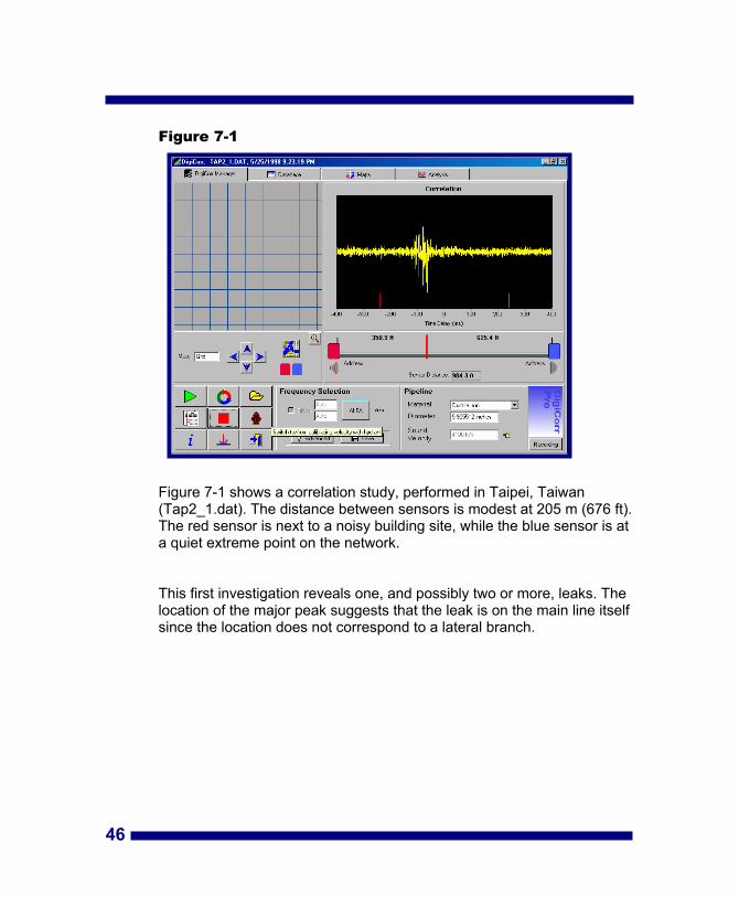
Figure 7-1

Figure 7-1 shows a correlation study, performed in Taipei, Taiwan (Tap2_1.dat). The distance between sensors is modest at 205 m (676 ft). The red sensor is next to a noisy building site, while the blue sensor is at a quiet extreme point on the network.

This first investigation reveals one, and possibly two or more, leaks. The location of the major peak suggests that the leak is on the main line itself since the location does not correspond to a lateral branch.

46

Figure 7-2

47

A subsequent study, shown in Figure 7-2 (Tap2_3.dat), was conducted between two valves 65 m apart, that is, with the sensors now closer to the suspected leak sites. This study confirmed that two distinct peaks, corresponding to positions 9 m apart on the main line, were reproducible. The positions of two leaks corresponding to the two largest peaks in the correlation function were confirmed.

There may be other leaks present in this section of pipeline. However, noise due to usage, flow, and in the environment may mask noise from other quieter leaks. If more leaks were suspected, an appropriate strategy would be first to repair the pipeline leaks detected and then to conduct another correlation study on the same section of mains.

48

7.2 Exploring the Advanced Features of the DigiCorr

to Pinpoint Difficult-To-Find Leaks

This section has been written to help you get the most out of the DigiCorr by showing clearly how to access its advanced features. In many situations the default settings of the DigiCorr (Filters: 200 to 2,000 Hz) reveal a leak automatically after a few seconds of data acquisition. This is often the case when the pipes under measurement are metal (all types of metal). The situation may be more challenging in any of the following circumstances:

1. The pipes under measurement are plastic (PVC or polyethylene). 2. Access points are limited or at a great distance. 3. Direct access to the pipeline where the leak is suspected is not

available (i.e. meters on service lines must be used or several sections of pipeline are traversed by the leak sound to reach the sensors).

4. Disturbances in the flow are present (i.e., at an intersection of

two mainline pipes). 5. Leak noise is not transmitted the entire distance between the

sensors (for example, if there is a complete break in the pipe or land subsidence has created a U shaped pipe with air in the depression).

6. Wide diameter pipes may have significant sound reflections

created by air in the pipe.

This tutorial deals with these and other measurement situations where interpretation of the correlation and successful pinpointing of the leak may require some effort. The tutorial may be read on its own or it may be advantageously followed sitting down with the program and running through the examples.

7.2.1 Multiple Leaks Identified in One Correlation Figure 7-3

49

Press the START button, select STORED DATA [F3], and open the file, Pen2.dat.

The filters are in their default position for metal pipes: 200 to 2,000 Hz. The stored leak noise data is read and the correlation develops for several seconds, concluding as in Figure 7-3.

There are 3 peaks in the correlation function:

1. The main peak (automatically detected) pinpoints a significant

leak. A peak as distinct as this, on a pipe of any material, is likely to be due to a leak if it develops consistently for a few seconds. A leak creates a point source of turbulent noise within the pipe. Since the pipe is (almost) a closed system, this leak noise has nowhere to travel but through the fluid in the pipe. This type of noise is uniquely coherent because it originates from turbulent flow within

50

the pipe. The correlator measures the difference in time of arrival of this leak sound at the yellow and blue sensors. The correlation graph displays this time difference, measured in milliseconds (thousandths of a second).

2. The second peak (to the right of the tallest peak) indicates a probable leak on a lateral line. This leak was confirmed after noting that a lateral line junction was present at position on the main pipeline predicted by the correlation result. The location of the leak can be immediately found by double clicking with the mouse pointer over the peak on the correlation graph.

3. The third peak (to the left) was considered to be probably due to usage. It was noted that a residence was located near the point on the pipeline corresponding to the peak. Repeated correlation studies did not always show a third peak. The third peak can be ruled out definitively by performing another correlation study after the repair of the first two leaks.

The noise level away from the peaks in the correlation function is low. This result is a typical example of what can often be achieved with iron (cast or ductile) or steel pipes. If the material and diameter of the pipe are known, and are consistent, then the inherent error in the correlation result is often on the order of a few inches to four feet over distances of up to 2,000 feet or more. 7.2.2 Frequency-Dependent Results in Correlation It is possible to adjust the digital filters to focus on the leak noise and to eliminate artifacts or disturbances. There are three possible strategies with digital filtering:

1. Choose a quiet part of the frequency spectrum of the pipe sound

to avoid artifacts; 2. Identify a portion of the spectrum that is coherent (plastic pipes); 3. Identify peaks in the spectrum that correspond to leak noise

(non-plastic pipes).

An example of each situation is shown in the next 3 subsections.

Elimination of Artifacts Figure 7-4

51

Press the START button, select STORED DATA [3], and open the file St-ga32.dat. The correlation function develops as shown in Figure 7-4.

There is no peak apparent in the correlation function. In this recording:

1. The correlation result is frequency sensitive.

2. The leak is directly under the yellow sensor.

Figure 7-5

52

Go to the ANALYSIS tab. In the RECORDED DATA panel make sure both the blue and the yellow boxes are checked and then push the “Go” button. Observe the sound intensity is much greater in the yellow channel than the blue due to the proximity of the leak.

If the sensor is directly over the leak (or very close), the leak sound wave may not be propagating in laminar flow at the sensor, which can disrupt the correlation function. In this example, spectral analysis is used to identify frequency ranges which contain large amounts of interference vibrations.

Still on the ANALYSIS tab, click on the ALFA button in the FREQUENCY SELECTION Panel and make sure the filters are set to 20 – 2,000 Hz. Then go to the SPECTRAL ANALYSIS Panel and make sure the scale is set to “Linear” and both the blue and the yellow boxes are checked. Press the REANALYZE button. The frequency spectra for the yellow and blue sensors are as shown in Figure 7-6.

Figure 7-6

There is significant energy at high frequencies in the yellow channel (800 Hz and greater). There is a stlow frequency component inthe blue channel. Selectfrequencies of 300 to 800 Hz for correlation will avoid these components of the

53

rong

ing

spectrum.

e

d other very loud noise sources, both

internal and external to the pipe.

CTION Panel to 300 – 800 Hz and then press the REANALYZE button.

n function computed between 300 and 800 Hz is hown in Figure 7-7.

NOTE: In this example we are following a strategy of correlating on th“quiet” part of the frequency spectrum because we suspect artifactual noise. The same strategy can also be used when there are pumps, louhighway or construction noise, or

Change the filter settings in the FREQUENCY SELE

After the correlation analysis has been repeated, the correlation functionhas a peak and the leak is identified as being 91.2 feet from the yellow sensor. The correlatios

54

igure 7-7

uency range is tried if a correlation has not been successfully obtained:

100 - 300 Hz

Spectral Coherence in Plastic Pipes

Plastic p

ction joints) which cause peaks to appear in the correlation

F Important With metal pipes the following frequency ranges have been found to be very effective. It has been suggested that each freq

200 - 2,000 Hz 300 - 800 Hz 250 - 450 Hz

ipes present special challenges to correlation due to:

Attenuation of the leak noise along the pipe length Vibration, resonance, or standing waves within the pipe

Properties of the pipe (e.g. se

8 DigiCorr Digital Mapping & Data Base

DigiCorr Pro is a computerized leakage management system which includes digital mapping and database modules in addition to all of the advanced features of the basic DigiCorr system. Leakage is tracked automatically, providing important and useful information to managers in easy to understand formats. Advanced analysis of acoustic data from the entire distribution system is possible in the field or in the office.

8.1 Digital Mapping Module

Distribution system maps are easily integrated into the DigiCorr Pro program allowing field crews to record sensor locations on the maps.

E

D

C

B

A

55

56

A. Thumbnail Panel – the red box shows the relative location of the map panel to the overall utility map

B. Map Control Panel – helps you navigate around the maps

C. The current map can be selected by clicking in the “Thumbnail

Panel” or by entering a map name

D. The map magnification can be increased or reduced using the Zoom buttons

E. Print the content of the Map Panel exactly as it appears on screen

8.2 HydroData Management Module

The DigiCorr HydroData Management module automatically saves every recording made with the DigiCorr system (either in the Field Recording Screen or the DigiCorr Manager Screen) in a special database. The database can be customized by adding new fields at any time. The file C:\Program Files\Flow Metrix\DB\DBInit.txt contains the name of the database file. This file can be edited using MS Excel or Access or any ODBC compliant database program. Any new fields added by the user become visible in DigiCorr Pro. Initially, the most recent 500 recordings are displayed in the database table: A. The user may enter an “Action” for any record. B. Click once on any row to highlight the record. C. Then click on the “Analysis” button to re-analyze that data.

(Double-clicking on any row will achieve the same results.) D. The “More” button appends the next 500 recordings to the

database table. E. The “Previous” button returns to the screen to the full database

after searching.

57

F. Any recording can be quickly located using the “Search” facility. Type in any text string, for example, “5/18/00”, “Main Street”, “L3”, or “ductile” to find all records that have an entry matching the text.

A

B

CDEF