usermanual for holostudiom4 2.6 -...

1

User Manual for HoloStudio M4 2.6.2

with HoloMonitor M4

HoloStudio 2.6.2

Software Manual

©2015 Phase Holographic Imaging AB

3

Contact us:

Phase Holographic ImagingScheelevägen 22SE-223 63 LundSweden

+46-(0)46-386080

[email protected]

www.phiab.se

4

mailto:[email protected]

Introduction to the HoloMonitorTM M4

The HoloMonitorTM M4 is a cell analyzer for adherentcells. It can count cells and analyze adherent cellmorphology and confluence. The HoloMonitorTM M4can also be used for longterm timelapse captureswhich do not harm the cells. Cells can be trackedthrough the timelapse capture, both for movementand for morphology. The HoloMonitorTM M4 is incubatorproof, allowing for experiments to be performed in acell culture incubator.

The HoloMonitorTM M4 uses digital holography. Thistechnique is based on measurements of how the cellsshift the phase of light that passes through the cells. Thiskind of live cell imaging does not require any kind oflabeling or staining.

The cells can be analyzed while growing undisturbed intheir usual cell culture vessel. The HoloMonitorTM M4works with most of the common cell culture vesselssuch as 6-well plates, petri dishes and IBIDI slides.

The HoloMonitor is equipped with a flat sample stage(Figure 1), which can be replaced with a manual XY-stage (Figure 2) or a motorized XYZ-stage (Figure 3).When the M4 is equipped with a motorized stage,samples are directed to move using the computer.

Introduction to HoloStudioTM

HoloStudioTM is a specially designed software forcapture and analysis of digital holographic imageswith the HoloMonitorTM M4. HoloStudioTM enables theuser to capture images both as single captures and astime-lapse captures.

The procedure is simple: the user captures images ofthe sample using the HoloMonitorTM M4, and the imageis analyzed in the software HoloStudioTM. The imagingprocedure does not affect the cells in any measurableway.

To simply count cells takes approximately one minute.Confluence measurements are performedsimultaneously. To analyze the cells for area, thicknessor other parameters, either the built in analysisfunctions can be used or the data can be exported asxml-files for further work in Excel or similar programs.Cell movement and morphology can be traced overtime through a timelapse sequence for both individualcells and for a cell population.

The raw data will remain intact, as all changes madeby the user only concern how the results are displayed.The changes do not affect the raw data.

Applications

Some applications have been described in applicationnotes, such as cell motility, cell death, cell cycle andtoxicology. The application notes are available on ourwebpage:http://www.phiab.se/publications/application-notes

5

Figure 1: The HoloMonitor M4 with a flat sample stage

Figure 2: The manual XY-stage

Figure 3: The HoloMonitor with a motorized XYZ-stage

Table of Contents

Introduction to the HoloMonitorTM M4...................................5Introduction to HoloStudioTM.............................................5Applications...........................................................................5Software Manual...................................................................8

HoloStudio M4 2.6 outline..........................................................9Main tabs overview...............................................................9Live Capture..........................................................................9Analyze Data..........................................................................9Main Viewing window...........................................................9Side windows.........................................................................9

Manual PART ONE, Quickguides............................................11Start up and calibrate the instrument................................12Time lapse capture..............................................................13Parallel timelapse captures.................................................14Cell counting and confluence..............................................15Proliferation studies ...........................................................16Morphology analysis...........................................................17Cell tracking........................................................................18Data backup.........................................................................19

Manual PART TWO, a user guide............................................20

1. Start up and Close down.......................................................201.1. Start up at room temperature......................................201.2. Start up in the incubator..............................................201.3. Calibration....................................................................20

1.3.1. When everything is well........................................201.3.2. If the calibration shows something amiss..............211.3.3. If the problems persist...........................................21

1.4. Close down....................................................................21

2. View live images ....................................................................222.1. Focusing .......................................................................22

2.1.1. Automatic versus manual focusing........................222.2. Focus a live holographic image using an M4 with a standard sample stage.........................................................232.3. Focus a live holographic image using an M4 with a manual XY-stage..................................................................232.4. Focus a live holographic image using an M4 with a motorized XYZ-stage..........................................................23

2.4.1. Focus the image semi-automatically.....................232.4.2. Focus the image manually.....................................23

2.5. Improve/calibrate the holographic image...................242.6. Move the sample stage..................................................242.7. Move, flip or zoom the holographic image in the MainViewing Window..................................................................242.8. Change the holographic image display.......................252.9. Change the holographic image coloring......................25

3. Capture images .....................................................................273.1. Store captured images..................................................273.2. Capture a single image.................................................273.3. Capture a time lapse sequence ....................................273.4. Creating a pattern of images to be captured in a sequence...............................................................................27

3.4.1. Select the wells to be captured..............................283.4.2. Select positions to be captured..............................283.4.3. Create identical capture patterns in all wells........283.4.4. Create random capture patterns............................293.4.5. Create patterns using the current position............293.4.6. Clearing the capture pattern.................................293.4.7. Settle time after stage movement...........................293.4.8. Capture the pattern...............................................29

3.5. Capture timelapses at several locations in parallel. . . .293.5.1. Storing Captured pattern timelapses in one group 303.5.2. Storing parallel timelapses in separate groups.....30

4. View captured images............................................................314.1. View an image...............................................................314.2. View a timelapse...........................................................314.3. View one position of several in a timelapse ................31

4.3.1. Capture pattern timelapse stored in single group. .314.3.2. Capture pattern timelapse stored in individual groups.............................................................................32

4.4. Move, flip or zoom the cell image ..............................324.5. Holographic image display...........................................32

4.5.1. Change the image display.....................................324.5.2.Change the image coloring....................................33

4.6. Move, flip or zoom the cell image................................344.7. Recalculate a holographic image.................................34

4.7.2. Recalculate the focus manually.............................344.7.1. Recalculate the focus automatically .....................344.7.3. Recalibrate a holographic image..........................354.7.4 Using a background hologram...............................35

5. Cell identification...................................................................365.1. Identify cells..................................................................36

5.1.1. Select an image.....................................................365.1.2. Automatic threshold settings.................................365.1.3. Adjust the cell identification..................................37

5.2. Make adjustments for single cells................................375.3. Save the cell identification settings..............................385.4. Change the image display............................................385.5. Image information........................................................39

6. Cell Tracking..........................................................................406.1. Start tracking cell movement.......................................40

6.1.1 Add image frames to the analysis...........................406.1.2. Select cells to be analyzed.....................................406.1.3. Displaying the cell tracking..................................40

6.2. Cell tracking warnings.................................................416.3. Adjusting the cell tracking...........................................41

6.3.1. Select the cell to be adjusted.................................416.3.2. Switch the tracking from one cell to another.........426.3.3. Discontinue a cell tracking...................................426.3.4. Continue a discontinued cell tracking...................426.3.5. Undo manual changes...........................................42

6.4. Tracking cell morphology............................................426.4.1 Display cell morphology parameters for individual cells.................................................................................426.4.2 Display different cell morphology parameters.......42

6.5. Export the tracking results..........................................43

7. Analyze and export data........................................................447.1. Measure distances directly in the currently viewed image....................................................................................447.2. Analyze results in plot..................................................44

7.2.1. Start a new analysis..............................................447.2.2. Remove data from plot .........................................45

7.3. Display results in scatter-plot.......................................457.3.1. Identify data points as cells ..................................467.3.2. Change the scatter-plot axis units.........................477.3.3. Change the scatter-plot axis display manually......477.3.4. Create, hide and delete plot regions......................47

7.4. Display results in histograms.......................................487.4.1. Change the histogram axis units...........................497.4.2. Change the histogram X-axis intervals manually. .497.4.3. Change the number of bins....................................49

7.5. Export plots and cell data............................................497.5.1. Export cell data.....................................................497.5.2. Save plots and histograms.....................................50

8. Cell Count .............................................................................518.1. Count cells.....................................................................518.2. Adjust the histogram proportions...............................528.3. Remove data from plot ................................................528.4. Export results................................................................52

6

9. Export images and movies....................................................539.1. Add and remove image frames ...................................539.2. Edit the images..............................................................53

9.2.1. Zoom, move or flip the image................................549.2.2. Adjust the image display.......................................549.2.3. Holographic image coloring.................................55

9.3. Create an AVI movie.....................................................559.4. Export images...............................................................56

10. Back up.................................................................................5710.1. Back up of individual projects, groups or frames.....5710.2. Back up of the entire database...................................57

11. Troubleshooting....................................................................5911.1. Live Imaging...............................................................59

11.1.1. The Live Capture tab is inactive..........................5911.1.2. It is impossible to focus the live image................5911.1.3. The cells are very bright and blurry, showing no inner structures...............................................................5911.1.4. The cell image is completely white......................5911.1.5. The cell image is black........................................5911.1.6. The live image focus was OK, but it slowly turned bad and now it can not be set again................................60

11.2. Capture........................................................................6011.2.1. The cell image in the Main Viewing window is white...............................................................................6011.2.2. The capture button is inactive..............................6011.2.3. In a series of captured images not all images were good................................................................................60

11.3. View Images................................................................6011.3.1. No image frames are visible in the Image Frame List window.....................................................................6011.3.2. The cell image in the Main Viewing window is white...............................................................................60

11.4. Cell Identification.......................................................6011.4.1. No image frames are visible in the Image Frame List window.....................................................................6011.4.2. The cell image in the Main Viewing window is white...............................................................................6011.4.3 The automatic cell identification looks strange... .6011.4.4. Some cells are incorrectly segmented as two or more................................................................................6011.4.5. Two cells are segmented as one...........................60

11.5. Analyze data................................................................6111.5.1. No image frames are visible in the Image Frame List window.....................................................................6111.5.2. The cell image in the Main Viewing window is white...............................................................................6111.5.3. The dots in the dot plot disappeared....................61

11.6. Cell Tracking...............................................................6111.6.1. The tracks are very irregular...............................61

11.7. Export images and movies..........................................6111.7.1. No image frames are visible in the Image Frame List window.....................................................................6111.7.2. The cell image in the Main Viewing window is white...............................................................................61

Addendum A: Morphological parameters...............................62Holographic microscopy ....................................................62

Holographic technology..................................................62Phase shift......................................................................62Threshold settings...........................................................62Note!...............................................................................62

Cell morphology parameters..............................................63References............................................................................64

Index.............................................................................................66

7

The Software Manual

In the first part of the manual there are quick guides tothe most common procedures such as cell counting,timelapse captures and cell tracking.

In the second part of the manual, there are detailedguides of how to perform different procedures usingHoloStudio, such as how to capture an image andhow to analyze the images.

The last chapter contains a trouble shooting guide.

8

HoloStudio M4 2.6 outline

Main tabs overview

HoloStudio M4 Tracking TM is divided into sevenfunctional parts that are represented in seven differenttabs (Figures 4 and 5):

1. Live Capture, which concerns the live viewingand capturing of digital hologram images.

2. View Images, which concerns viewingcaptured images.

3. Identify Cells, which concerns thesegmentation of the image, resulting in theidentification and outlining of the cells.

4. Track Cells, which concerns the tracking ofindividual cells through a series of capturedframes.

5. Analyze Data, which concerns the analysis ofcells in the captured hologram images, as wellas display and export of the results.

6. Cell Count, which concerns the counting ofadherent cells in their cell culture vessels.

7. Export Images, which concerns thevisualization and export of images and movies.

The Main Viewing window

The Main Viewing window (Figure 5) shows the actuallive cell image when the Live Capture tab is open andwhen the other tabs are open it shows the currentlyselected stored image.

The Side windows

Basic functions are found in side windows to the leftand right of the Main Viewing window (Figure 5). If theside windows are collapsed they can be expanded byclicking the black arrow tip found in every side windowheader.

Additional functions or parameters are found in theMore menus in some of the side windows. Thesefunctions are usually not needed for the user but ratherfor the service engineers.

Information concerning the different side windows canbe found by clicking the Information buttons which areplaced in the side window headers (Figure 6).

9

Figure 4: The main tabs of HoloStudio 2.6

10

Figure 6: Information button

Figure 5: Overview of a main tab

Main tabs

Main Viewing window

Side windows

Manual PART ONE

Quick guides to commonlyused procedures

Quick guides index

Start up and Calibrate the instrument...........................................12

Time lapse capture and export.....................................................13

Parallel timelapse captures..........................................................14

Cell counting and confluence measurements ..............................15

Proliferation studies ....................................................................16

Morphology analysis...................................................................17

Cell tracking in a timelapse ........................................................18

Data backup.................................................................................19

11

Quick guide: Start up and calibrate the instrument

Putting the instrument in the incubator

1. Put the HoloMonitor M4 in the incubator

and immediately attach all cords. The

instrument must be connected to the wall

socket at all times when placed in the

incubator.

2. Wait 3-4 hours for the instrument

temperature to stabilize.

Startup

3. Start the laser 30 minutes prior to use.

4. Start the computer.

5. Start HoloStudio.

Calibration at start up

6. Go to the Live Capture tab.

7. The Calibration Wizard window will appear.

8. Follow the instructions of the wizard to

perform a calibration.

9. If all values are in the green everything is

ready to go.

Calibration at other timepoints

10. To calibrate at other timepoints, select the

Help-option, and then Calibration wizard in

the top menu.

11. Proceed as above.

Troubleshooting

12. If any values are in the red, check the

following:

13. All cables and connections are correctly

attached.

14. There is laser light.

15. The objective and the small laser window

are clean.

16. Recalibrate.

Collect diagnostics

17. If problems persist, collect diagnostics by

selecting the Help-option, and then Collect

Diagnostics in the top menu. Follow the

instructions of the Collect Diagnostics

Wizard.

12

Quick guide:Time lapse capture and movie export

Startup

1. Make sure that the instrument has been

placed in an incubator for at least three

hours while switched on. If the instrument is

to be operated at room temperature, start

the HoloMonitor 30 minutes prior to use.


3. Start HoloStudio M4.

Image capture


5. Choose/create a project and a group.

6. Put the cell sample on a spacer plate or

vessel holder of the correct type. Make sure

the image is focused.

7. Activate the Timelapse function and enter

the total time and the interval between the

time points.

8. Press Capture.

9. Use the View Images tab to ensure that the

captured imges correspond to your settings.

10. When image capture is complete, proceed

to the View Images tab.

11. Run through your images by clicking the

Autoscroll button. If needed, recalculate

the images.

Export individual images or a movie

12. Go to the Export Images tab.

13. Highlight or check the image frames you

want to include in the movie or image

export.

14. Click the Add buttons in the lower right

corner of the program to add the data

from the highlighted or checked image

frames.

15. Adjust the coloring and viewing angles of

the added images.

16. Preview the movie.

Export Images or movies.

13

Quick guide:Parallel timelapse captures


placed in an incubator for at least three hours

while switched on. If the instrument is to be

operated at room temperature, start the

HoloMonitor 30 minutes prior to use.



Image capture

4. Open the Live Capture tab.

5. Put the cell sample on a spacer plate or vessel

holder of the correct type. Make sure the

image is focused.

6. Choose capture positions in the sample/s. First

select a suitable vessel in the Stage position-

box. Find an interesting position for imaging.

Click on Remember in the Stage position-box.

Repeat for as many positions as required.

7. Create a project and groups for the parallel

timelapses. First tick the Capture pattern-

checkbox in the Capture-box. Then click on

Setup storage which will show the Configure

destinations-window. Select a project and

then tick the Multiple destination groups-

checkbox. Click OK.

8. Press Capture.



10. When image capture is complete, proceed to

the View Images tab. Run through your images

by clicking the Autoscroll button. If needed,

recalculate the images.

Export individual images or a movie

11. Go to the Export Images tab.

12. Highlight or check the image frames you want

to include in the movie or image export.

13. Click the Add buttons in the lower right corner

of the program to add the data from the

highlighted or checked image frames.

14. Adjust the coloring and viewing angles of the

added images.

15. Preview the movie.

16. Export Images or movies.

14

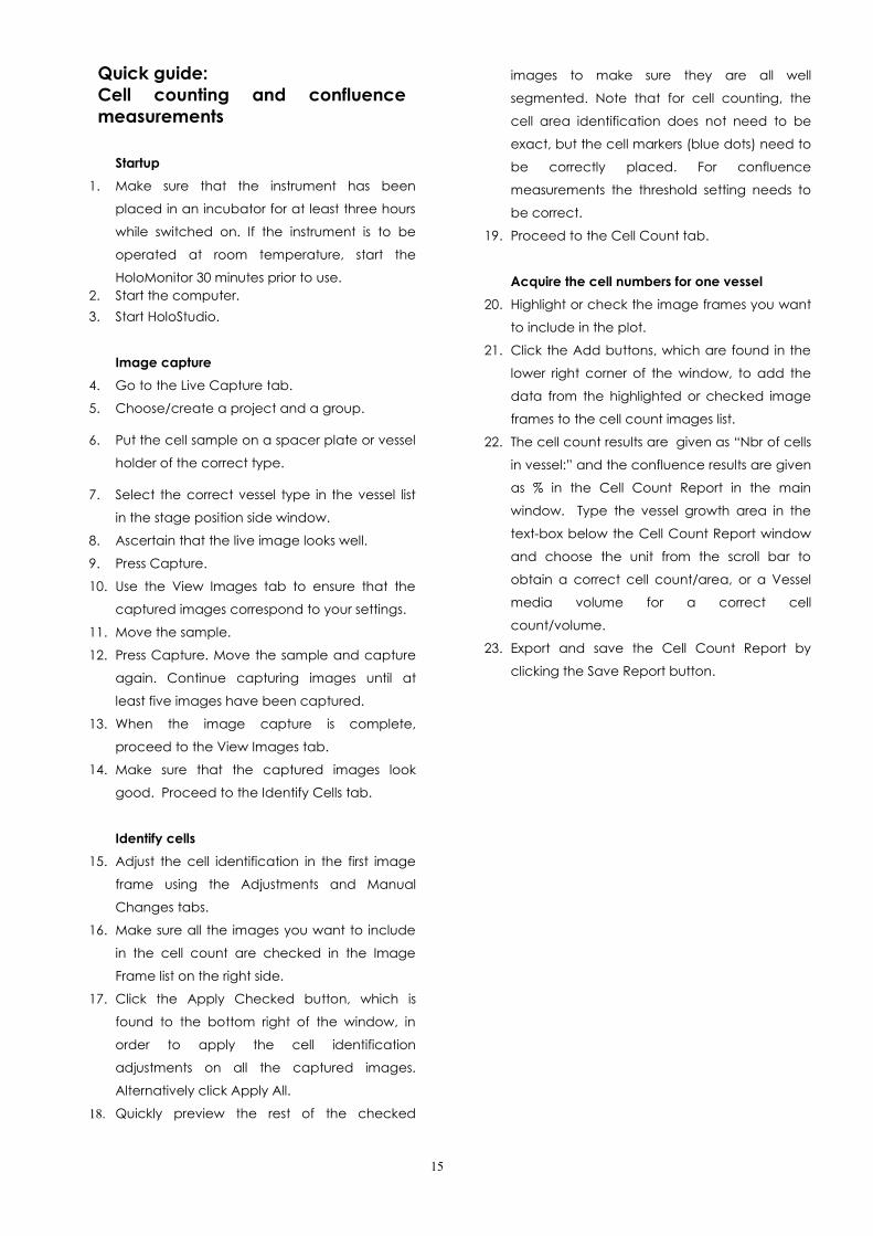
Quick guide:Cell counting and confluencemeasurements

Startup





HoloMonitor 30 minutes prior to use.2. Start the computer.


Image capture




holder of the correct type.

7. Select the correct vessel type in the vessel list

in the stage position side window.

8. Ascertain that the live image looks well.

9. Press Capture.


captured images correspond to your settings.

11. Move the sample.

12. Press Capture. Move the sample and capture

again. Continue capturing images until at

least five images have been captured.

13. When the image capture is complete,

proceed to the View Images tab.

14. Make sure that the captured images look

good. Proceed to the Identify Cells tab.

Identify cells

15. Adjust the cell identification in the first image

frame using the Adjustments and Manual

Changes tabs.

16. Make sure all the images you want to include

in the cell count are checked in the Image

Frame list on the right side.

17. Click the Apply Checked button, which is

found to the bottom right of the window, in

order to apply the cell identification

adjustments on all the captured images.

Alternatively click Apply All.

18. Quickly preview the rest of the checked

images to make sure they are all well

segmented. Note that for cell counting, the

cell area identification does not need to be

exact, but the cell markers (blue dots) need to

be correctly placed. For confluence

measurements the threshold setting needs to

be correct.

19. Proceed to the Cell Count tab.

Acquire the cell numbers for one vessel


to include in the plot.

21. Click the Add buttons, which are found in the

lower right corner of the window, to add the

data from the highlighted or checked image

frames to the cell count images list.

22. The cell count results are given as “Nbr of cells

in vessel:” and the confluence results are given

as % in the Cell Count Report in the main

window. Type the vessel growth area in the

text-box below the Cell Count Report window

and choose the unit from the scroll bar to

obtain a correct cell count/area, or a Vessel

media volume for a correct cell

count/volume.

23. Export and save the Cell Count Report by

clicking the Save Report button.

15

Quick guide:Proliferation studies

Startup








Image capture






8. Press Capture.




11. Press Capture. Continue until at least five

images have been captured.





Identify cells



Changes tabs.

15. Make sure all your images are checked in the

Image Frame list on the right side.

16. Click the Apply checked button, which is

found to the bottom right of the window, in

order to apply the cell identification

adjustments on all the captured images.

17. Quickly preview the rest of the images to

make sure they are all well segmented. Note

that for cell counting, the cell area

identification does not need to be exact, but

the cell markers (blue dots) need to be

correctly placed. For confluence

measurements the threshold setting needs to

be correct.

18. Proceed to the Cell Count tab.

Acquire the cell numbers for one vessel



20. Click the Add buttons, which are found in the

lower right corner of the window, to add the

data from the highlighted or checked image

frames to the cell count images list.

21. The cell count results are given as “Nbr of cells

in vessel:” and the confluence results are given

as % in the Cell Count Report in the main

window. Type the vessel growth area in the

text-box below the Cell Count Report window

and choose the unit from the scroll bar to

obtain a correct cell count/area, or a Vessel

media volume for a correct cell

count/volume.

22. Export and save the Cell Count Report by

clicking the Save Report button.

Acquire cell numbers for several vessels at

several time points

23. Repeat points 6-11 and 12-22 for each cell

culture vial and for each measuring time point.

24. To compare data from different time points,

note the cell number and standard deviation

values found in the Cell count report in an

Excel sheet.

16

Quick guide:Morphology analysis

Startup





HoloMonitor 30 minutes prior to use.2. Start the computer.


Image capture








9. Press Capture.











Identify cells



Changes tabs.


Image Frame List window on the right side.

17. Click the Apply checked button to the bottom

right of the program in order to apply the cell

identification adjustments on all the captured

images. Alternatively, click apply All.


make sure they are all well segmented.

19. Proceed to the Analyze data tab.

Data analysis using HoloStudio

20. Click New analysis to start a new project.





highlighted or checked image frames to the

plot.

23. Create plots showing the cell morphology by

using the X- and Y-axis labels of interest.

24. If necessary, add regions to gain separate

data for the included cells, in addition to the

complete data-set.

External data analysis

25. Go to the Export tab, below the Main Viewing

window. Click the Export data button to save

the cell data of all added image frames to an

xml-file at a location of your choice.

26. Open the data-sheet in a spreadsheet

program of choice.

27. Analyze the parameters of interest.

17

Quick guide:Cell tracking in a timelapse

Startup








Image capture








9. Press Capture.











Identify cells



Changes tabs.


Image Frame list on the right side.

17. Click the Apply checked button to the bottom

right of the program in order to apply the cell

identification adjustments on all the captured

images. Alternatively, click Apply All.


make sure they are all well segmented. Adjust

the segmentation as needed.

19. Proceed to the Track Cells tab.

Track cells through the timelapse

20. Click the button for New Analysis.


to include in the tracking.



highlighted or checked image frames.

23. Activate the Add Cells function in the Select

Mode side window. Add cells to be tracked by

clicking them.

24. Follow the tracking by using the Timeline which

is found below the Cell tracking window.

Spatial tracking

25. Select the Plot Movement tab, which is found

behind the Tracking tab. The directions of the

cell movements are given in a diagram.

Morphological tracking

26. Select the plot Features tab, which is found

behind the Tracking and Plot Movements tabs.

The Area over time is given as a default. To

view other morphological parameters, select a

different feature in the cell features list which is

found below the diagram.

Export tracking data

27. Select the Tracking tab and click export to

create an xml-file containing all the tracking

data.

28. The cell tracking image containing the tracks

can be saved by using the snapshot button in

the Tracking tab.

29. The spatial tracking diagrams can be exported

by using the Export Plot button in the Plot

Movement tab.

18

Quick guide:Data backup

Backup of individual projects, groups or

frames

1. Click Database in the top menu.

2. Go to Export.

3. When the browser window opens, create a

new folder at the selected destination.

4. Select the projects, images or groups that you

want to export/back up.

5. Click Export.

Backup of the entire database folder

6. Click Database in the top menu.

7. Click Settings.

8. Determine the Root Directory for the database

folder HstudioimageDB. This is a road map to

find the folder.

9. Go to HstudioimageDB.

10. Copy the entire HstudioimageDB folder.

19

Manual PART TWOA user guide

Chapter 1. Start up and Close down.

1.1. Start up at room temperature

• Switch on the laser and the instrument. Itneeds 15 minutes of pre-warming beforethe laser is stable.

• Start the computer.• Open HoloStudio.

If you want to work with HoloStudio without using theinstrument:


When HoloStudio is not connected to an instrumentthe Live Capture tab will be inactive.

1.2. Start up in the incubator

• Put the M4 instrument in the incubator andconnect all cords. The electricity must beconnected when the instrument is in theincubator, otherwise there will be acondensation problem.

• Wait 3-4 hours for the instrumenttemperature to stabilize.

• Switch on the laser. It needs 15 minutes ofpre-warming before the laser is stable.


1.3. Calibration

The first time the Live Capture tab is selected afterstarting the software with an instrument connected, a

Calibration Wizard window will appear (Figure 7).The wizard can also be accessed from the Help-optionin the Top Menu (Figure 8) or from the Calibration sidewindow (Figure 9).

When the instructions of the wizard are followed, theinstrument will be calibrated. Do this every time theinstrument is started or if it has been running for a longtime.

1.3.1. When everything is well

If the calibration is successful, all parameters necessaryto achieve good imaging are within their bounds. Awindow will appear to inform about the successfulcalibration of objective and background (Figure 10). Thereafter the Calibration Wizard will show the status ofthree important parameters (Figure 11). Click the Closebutton to exit from the Calibration Wizard. Valuesshown to be in the green are excellent, and values inthe yellow are acceptable.

20

Figure 7: The Calibration Wizard

Figure 8: The Calibration wizard in the top menu

Figure 9: The Calibration wizard in the Calibration side window

Figure 10: The Calibration Wizard showing a successful calibration of objective and background

1.3.2. If the calibration shows something amiss

If there is a problem with the calibration a warningwindow will appear (Figure 12). When the OK buttonhas been clicked, a window showing diagnosticsvalues in the red will appear (Figure 13).

If any values are in the red and the calibration couldnot be performed, check the following:

• That all cables and connections are correctlyattached.

• That there is laser light.• That the blue laser fiber is not pinched down,

bent or pulled in any way.

• That the objective and the small laser windoware clean, otherwise clean with a cotton swabdipped in ethanol.

Then recalibrate using the Recalibrate button (Figure13).

1.3.3. If the problems persist

If problems persist, collect diagnostics by selecting theHelp-option, and then Collect Diagnostics in the topmenu (Figure 14). Follow the instructions of the CollectDiagnostics Wizard (Figure 15).

1.4. Close down by using the on/off switch on theinstrument and by closing the computer program.

For further information concerning the handling of theHoloMonitor M4, please use the Getting Started guide.

21

Figure 12: The Calibration Warning window

Figure 13: The Calibration Wizard after an unsuccessful calibration

Figure 15: The Collect Diagnostics Wizard

Figure 14: The Collect Diagnostics Wizardin the top menu

Figure 11: The Calibration Wizard after a successful calibration

Chapter 2. View live images

Select the Live Capture tab (Figure 16).

2.1. Focusing

There are two different focusing mechanisms thatneed to cooperate in order for the image to be infocus. With the hardware focus the user places thecells to be viewed at the approximately correctdistance from the objective. The software focusdescribes how well the computer is able to calculatean image based on the light information that reachesthe sensor.

Put the cell sample on the stage. An image will appearin the Main Viewing window. If the image is correctlyfocused, the green bar in the Software Focus sidewindow will be in the green area (Figure 17).

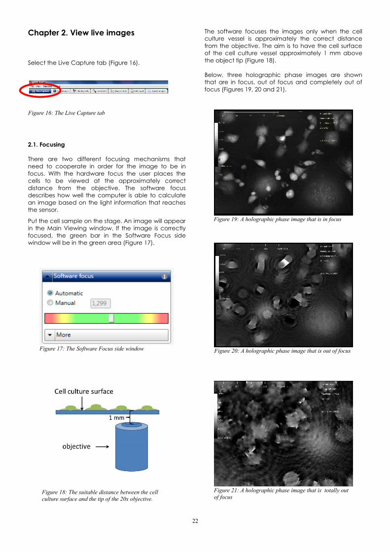
The software focuses the images only when the cellculture vessel is approximately the correct distancefrom the objective. The aim is to have the cell surfaceof the cell culture vessel approximately 1 mm abovethe object tip (Figure 18).

Below, three holographic phase images are shownthat are in focus, out of focus and completely out offocus (Figures 19, 20 and 21).

22

Figure 16: The Live Capture tab

Figure 19: A holographic phase image that is in focus

Figure 20: A holographic phase image that is out of focus

Figure 21: A holographic phase image that is totally out of focus

Figure 17: The Software Focus side window

Figure 18: The suitable distance between the cell culture surface and the tip of the 20x objective.

2.1.1. Automatic versus manual focusing

Automatic focusing mostly results in well focusedimages. Some cell samples are more demanding andneed to be focused manually. Check Manual in theSoftware Focus side window (Figure 22).

The text box next to the Manual button shows thecurrent software focus distance in mm. That distancecan be set to a different value either by entering avalue manually or by using the colored slide barbeneath the text box. Move the slide bar until theimage looks good.

2.2. Focus a live holographic image using an M4 with astandard sample stage

Choose the correct spacer plate and put it on thestage. Then put the cell sample on the stage. Animage will appear in the Main Viewing window. If theimage is correctly focused, the slide bar in theSoftware Focus side window will be in the green area(Figure 17).

The thicker the plate, the further away from theobjective the sample will be. Essentially, the image isfocused if the correct distance plate is used. If theimage is out of focus, try a different distance plate or adifferent combination of plates until the software focusis in the middle of the green.

2.3. Focus a live holographic image using an M4 with amanual XY-stage

The manual XY-stage is delivered with holders forstandard cell culture vessels. If the correct holder isselected, and then the vessel is placed on the stage,the cells will be in focus.

2.4. Focus a live holographic image using an M4 with amotorized XYZ-stage

The motorized XYZ-stage is delivered with holders forstandard cell culture vessels.

2.4.1. Focus the image semi-automatically

Place the sample on the stage. Wait for the image tostabilize. Make sure that Automatic is activated in theSoftware Focus side window (Figure 17).

Adjust the hardware focus using the MicroscopeSettings side window (Figure 23) which is found to theright of the Main Viewing window (Figure 5).

To the left in the Microscope Settings side windowthere is an objective representation and a black barthat represents the sample stage (Figure 23). Thehardware focus distance can be adjusted in largesteps by left clicking, holding and moving the blackbar with the mouse cursor. This allows the stage to bemoved up and down. The distance between theobjective and the sample is shown in the Focus textbox.

To the right in the Microscope Settings side windowthere is a double gray wheel with red knobs which isused for intermediate (outer wheel) and small (innerwheel) focus adjustment steps. The wheels are movedby left clicking, holding and moving the red knobs.

Keep adjusting the focus until the white rectangle inthe color bar in the Software Focus side window(Figure17) is placed in the center of the green area ofthe color bar. The hardware focus is now set to allowthe software focus to operate optimally.

When using the 20x objective, the aim is to have thecell culture surface 1 mm above the objective tip(Figure 18).

2.4.2. Focus the image manually

Automatic focusing mostly results in well focusedimages. Some cell samples are more demanding andneed to be focused manually. Check Manual in theSoftware Focus side window (Figure 24).

The text box next to the Manual button shows thecurrent software focus distance in mm. That distancecan be set to a different value either by entering a

23


Figure 23: The Microscope Settings side window

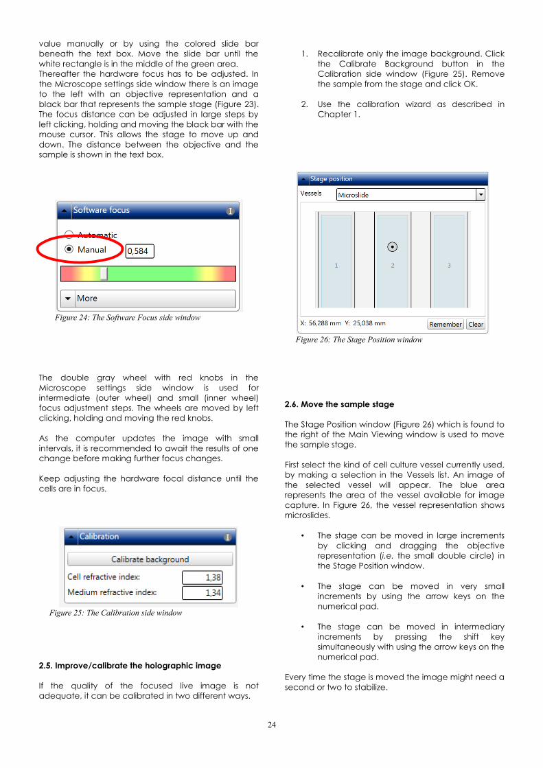
value manually or by using the colored slide barbeneath the text box. Move the slide bar until thewhite rectangle is in the middle of the green area.Thereafter the hardware focus has to be adjusted. Inthe Microscope settings side window there is an imageto the left with an objective representation and ablack bar that represents the sample stage (Figure 23).The focus distance can be adjusted in large steps byleft clicking, holding and moving the black bar with themouse cursor. This allows the stage to move up anddown. The distance between the objective and thesample is shown in the text box.

The double gray wheel with red knobs in theMicroscope settings side window is used forintermediate (outer wheel) and small (inner wheel)focus adjustment steps. The wheels are moved by leftclicking, holding and moving the red knobs.

As the computer updates the image with smallintervals, it is recommended to await the results of onechange before making further focus changes.

Keep adjusting the hardware focal distance until thecells are in focus.

2.5. Improve/calibrate the holographic image

If the quality of the focused live image is notadequate, it can be calibrated in two different ways.

1. Recalibrate only the image background. Clickthe Calibrate Background button in theCalibration side window (Figure 25). Removethe sample from the stage and click OK.

2. Use the calibration wizard as described inChapter 1.

2.6. Move the sample stage

The Stage Position window (Figure 26) which is found tothe right of the Main Viewing window is used to movethe sample stage.

First select the kind of cell culture vessel currently used,by making a selection in the Vessels list. An image ofthe selected vessel will appear. The blue arearepresents the area of the vessel available for imagecapture. In Figure 26, the vessel representation showsmicroslides.

• The stage can be moved in large incrementsby clicking and dragging the objectiverepresentation (i.e. the small double circle) inthe Stage Position window.

• The stage can be moved in very smallincrements by using the arrow keys on thenumerical pad.

• The stage can be moved in intermediaryincrements by pressing the shift keysimultaneously with using the arrow keys on thenumerical pad.

Every time the stage is moved the image might need asecond or two to stabilize.

24

Figure 25: The Calibration side window

Figure 26: The Stage Position window


2.7. Move, flip or zoom the holographic image in theMain Viewing Window

To zoom the live image, left click the image in the MainViewing window (Figure 5) and then use the mousescroll button.

To move the live image to a desired location in theMain Viewing window, click, hold and drag the imageusing the left mouse button.

To flip and move the live 3-D image, click, hold anddrag the image using the right mouse button.

2.8. Change the holographic image display

To change how the live holographicimage is displayed, open the Viewer Options sidewindow (Figure 27) on the left hand side of the MainViewing window (Figure 5).

By clicking the Center button (Figure 28) the image willbe centered in the Main Viewing window.

By pressing the Snapshot button an image of thecurrent view will be saved (Figure 29).

Different image display options are shown (Figure 27).They can be activated by checking the boxes. Someboxes can be checked in parallel, thus making itpossible to combine functions.

• Checking FFT (Figure 27) displays the FastFourier Transform which represents thefrequency domains.

• Checking Uncut displays the image as it is firstreconstructed.

• Checking Laser Pattern displays the originalinterference pattern resulting from the mergingof the object and reference laser beams.

• Checking Hologram displays the reconstructedimage which is based on the laser pattern. Thehologram can be displayed showing either thephase or amplitude information of the lightwave.

• Checking Phase displays the light wave phaseinformation in the hologram.

• Checking Amplitude displays the light waveamplitude information in the hologram.

• Checking 3-D displays the holographic data asa 3-dimensional representation.

• Checking Rotate auto-rotates the image.

• Checking Show Ruler displays a horizontalscale bar representative of the distance in Xand Y.

• Checking Show Color Bar (Figure 27) displays avertical scale bar representative of the heightin Z.

• Checking Light Effect applies an artificial lightsource to the image which may sometimesrender an improved image.

• Checking Shiny Surface applies an artificiallight source to the image which maysometimes render an improved image. ShinySurface is only visible when Light Effect ischecked.

2.9. Change the holographic image coloring

All images originally appear in gray scale. If colors areneeded or wanted, use the Coloring side window(Figure 30) to the left of the Main Viewing window(Figure 5).

A set of colors that are saved together is called aColorset. A previously saved Colorset can be used withthe current image by making a selection in theColorset list which is found at the top of the Coloringside window (Figure 30).

25

Figure 27: The Viewer Options window

Figure 28: The Center button

Figure 29: The Snapshot button

• By left clicking the R-button (Figure 31) thecoloring in the image is rescaled to betterutilize the optimal dynamic range of theimage. This button needs to be operatedevery time the image coloring is off.

• A new color can be added to the colorset byclicking the plus button (Figure 31) and selecta new color. A colored triangle representingthe new color will appear beneath thehistogram (Figure 30). Alternatively, right clickon the X-axis and select Add Color.

• Change the color by using the right mousebutton to click on a colored triangle beneaththe histogram and select a new color,alternatively left click the arrow button andselect Change Color (Figures 30 and 31).

• To change the color span, left click and movethe desired colored triangle beneath thehistogram using the cursor (Figure 30).

• To save a new colorset with the current colorsettings, left click the arrow button and chooseSave As (Figure 31).

• To save the current color settings to apreviously saved colorset, left click the arrowbutton and choose Save (Figure 31). Note thatthis will overwrite the settings previously savedto this colorset.

• To delete a colorset, select it in the Colorset listby left clicking it. Then left click the arrowbutton and select Delete Colorset (Figure 31).

26

Figure 30: The Coloring side window

Figure 31. Coloring side window functions

Chapter 3. Capture images

Note that only holographic phase representations canbe captured! If e.g. an FFT image is desired, please usethe snapshot button in the Viewer Options side window(Figures 27 and 29).

3.1. Store captured images

Select the Live Capture tab (Figure 32) Before imagescan be captured, a place of storage must beprepared. The images must be stored in a Group withina Project. Either open an existing project or create anew project in the Capture window (Figure 33). Thenopen an existing group or create a new group wherethe images will be saved.When a new project or group is created, the date andtime are automatically included in the name.

3.2. Capture a single image

Put the cell sample on the stage. A live image willappear in the Main Viewing window. Ascertain thatyou are satisfied with the quality of the live image (SeeChapter 2).

Click the Capture button.

The Capture button is inactive unless a project and agroup have been selected (Figure 34).

3.3. Capture a time lapse sequence

To enable slow events to be recorded and studied, amovie can be created from images captured atintervals, i.e. a timelapse movie.

In order to capture images for a timelapse study,check the Timelapse box (Figure 35) in the Capturewindow. Enter the total time for the timelapse andselect the desired time unit (seconds, minutes or hours).Enter the interval between the capture time points andselect the desired time unit (seconds, minutes or hours).The minimum interval between captures is given to theright of the interval time unit box.

The number of timepoints will be given when total timeand interval are entered.

Click the Capture button.

3.4. Creating a pattern of images to be captured in asequence

When it is necessary to capture several images in asequence, e.g. for cell counting purposes or for paralleltimelapses, it is convenient to create a capture

27

Figure 32: The Live Capture tab

Figure 34: The Capture window with an inactive Capturebutton

Figure 35: Activated Timelapse function

Figure 33: The Capture window

pattern. When this capture pattern is applied, theinstrument automatically captures the set number ofimages in the set pattern.

Check the Capture Pattern box (Figure 36) in theCapture side window.

3.4.1. Select the wells to be captured

Click the Selection button (Figure 36). This will make theCapture Pattern window appear, displaying arepresentation of the currently selected type of cellculture vessel (Figure 37). If necessary, change thecurrent type of vessel in the Stage Position window(Figure 38).

Even if the selected type of vessel contains only onewell, start by activating the Select Wells button (Figure39) and then click the wells. In the example below(Figure 40), the wells A2 and A3 will be captured, butnot A1 and B1-3 as they are not selected.

3.4.2. Select positions to be captured

Activate the Select Positions button (Figure 39) toselect the capture points. Select the capture points byclicking in the well representations. The selected pointswill be shown as red dots (Figure 40).

3.4.3. Create identical capture patterns in all wells

To create identical capture patterns in each of severalwells, check the box for Identical Patterns in Each Well(Figure 39). Now, every added capture point willappear in all selected wells.

28

Figure 37: Capture Pattern window showing selected wells

Figure 36: Activated Capture Pattern function

Figure 39: Activated Selection function

Figure 38: Change vessel type in the Stage position window

3.4.4. Create random capture patterns

To generate random capture patterns, first fill in thenumber of capture points in the text box and then clickthe Generate button (Figure 39).

Identical Patterns in Each well and the generation ofrandom capture points can be combined to generaterandom patterns that are identical in the selectedwells.

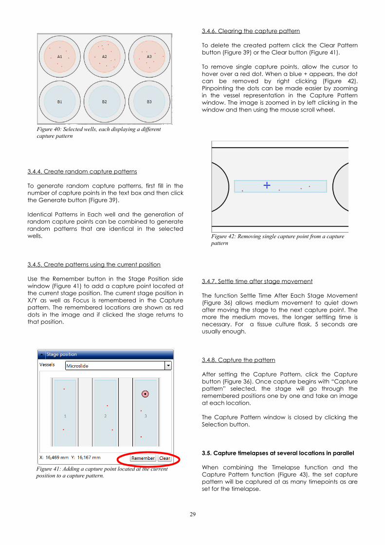
3.4.5. Create patterns using the current position

Use the Remember button in the Stage Position sidewindow (Figure 41) to add a capture point located atthe current stage position. The current stage position inX/Y as well as Focus is remembered in the Capturepattern. The remembered locations are shown as reddots in the image and if clicked the stage returns tothat position.

3.4.6. Clearing the capture pattern

To delete the created pattern click the Clear Patternbutton (Figure 39) or the Clear button (Figure 41).

To remove single capture points, allow the cursor tohover over a red dot. When a blue + appears, the dotcan be removed by right clicking (Figure 42).Pinpointing the dots can be made easier by zoomingin the vessel representation in the Capture Patternwindow. The image is zoomed in by left clicking in thewindow and then using the mouse scroll wheel.

3.4.7. Settle time after stage movement

The function Settle Time After Each Stage Movement(Figure 36) allows medium movement to quiet downafter moving the stage to the next capture point. Themore the medium moves, the longer settling time isnecessary. For a tissue culture flask, 5 seconds areusually enough.

3.4.8. Capture the pattern

After setting the Capture Pattern, click the Capturebutton (Figure 36). Once capture begins with “Capturepattern” selected, the stage will go through theremembered positions one by one and take an imageat each location.

The Capture Pattern window is closed by clicking theSelection button.

3.5. Capture timelapses at several locations in parallel

When combining the Timelapse function and theCapture Pattern function (Figure 43), the set capturepattern will be captured at as many timepoints as areset for the timelapse.

29

Figure 40: Selected wells, each displaying a different capture pattern

Figure 42: Removing single capture point from a capture pattern

Figure 41: Adding a capture point located at the current position to a capture pattern.

3.5.1. Storing Captured pattern timelapses in onegroup

By default all captures will be stored in the samegroup. This becomes impractical if the intention is tocapture a time-lapse at each location.

3.5.2. Storing parallel timelapses in separate groups

When using Capture pattern, the option to createseparate groups for each location is available. This isdone by clicking on Setup storage (Figure 36) whichwill show a configuration window (Figure 44).

In the Configure Destinations window, deafault is set toadding all captured frames into a single group. Whenchecking Multiple destination groups, the images will

be sorted into one group for each capture position(Figure 44). The group name can be set to either a newgroup or to an existing one. The default is to createnew groups. There will be an automatic suggestion ofthe group name, but it is also possible to name thegroups manually. It is possible to mix new and existinggroups. Click OK to save all groups.

In short:1. Click in the vessel image or use numeric arrow

keys to find an interesting position. 2. Click on Remember in the Stage position-box.

Every time you click Remember a captureposition is saved at the current XYZ-location.

3. Repeat 1-2 for as many positions as required.Tick the Capture pattern-checkbox in theCapture-box.

4. Click on Setup storage which will show theConfigure destinations-window.

5. Select a project and then tick the Multipledestination groups-checkbox.

6. Change group names if needed or click OK toaccept. The new groups will be created.

7. Select Time lapse in the Capture-box andenter duration and interval.

8. Click Capture.

The capturing process will begin and the resulting time-lapse images will be stored in the configured groups.

30

Figure 43: A combined timelapse and capture pattern capturing sequence

Figure 44: The Configure Destination window

Chapter 4. View captured images

In order to view and adjust captured images, selectthe View Images tab (Figure 45).

4.1. View an image

Start by selecting a Project and a Group in the ImageFrame List side window (Figure 46), which is found tothe right of the Main Viewing window.

An image frame presentation list for the selectedgroup will appear. Both holographic images andphase contrast images are presented in the list as wellas information pertaining to the images. Highlightingan image will make it appear in the Main Viewingwindow.

4.2. View a timelapse

Start by selecting a Project and a Group in the ImageFrame List side window (Figure 46), which is found tothe right of the Main Viewing window. Highlight the firstframe in the Image Frame List side window.

Below the Image Frame list there is an Auto Scrollbutton (Figure 48). Click that button to show the imageframes as a movie.

4.3. View one position of several in a timelapse

4.3.1. Capture pattern timelapse stored in single group

When a timelapse has been captured at severaldifferent positions in parallel using the motorized stageand then stored in a single group, it is possible to viewthe timelapse for each position separately.

The images in the Image Frame List will be arranged inorder of capture. If e.g. seven positions have beenselected, every seventh frame will belong to thetimelapse of that position.

First highlight the first of the images at the chosenposition. Then right click in the Image Frame List, selectCheck and thereafter Check every X frame (Figure 47).In the above example 7 would then be entered in theCheck Frames window (Figure 49). After clicking OK,check the Only Checked option found below theImage Frame List (Figure 48). Now, only the checkedimages will be displayed when Auto scrolling.

It is possible to select Check frames with comment asan alternative (Figure 47). That allows you to search fora comment such as the particular location XY-coordinate that was saved with the image (Figure 49).

31

Figure 45: The View Images tab

Figure 46: The Image Frame List side window

Figure 48: The Auto-Scroll button

Figure 47: The Check function

Figure 49: The Check Frames window

4.3.2. Capture pattern timelapse stored in individualgroups

For each position in the multi-position timelapse,images were stored in a separate group. Go to thegroup of interest. Highlight the first frame in the ImageFrame List side window.

Below the Image Frame list there is an Auto Scrollbutton (Figure 48). Click that button to show the imageframes as a movie.

4.4. Move, flip or zoom the cell image

To zoom the cell image, click the image in the MainViewing window and then use the scroll button on themouse.

To move the cell image to a desired location in theMain Viewing window, click, hold and drag the imageusing the left mouse button.

To flip and move a holographic 3-D image, click, holdand drag the image using the right mouse button onthe image.

4.5. Holographic image display

All holographic images will basically appear in grayscale and in 2-D, unless artificial coloring has beenchosen and the image display is set to 3-D.

4.5.1. Change the image display

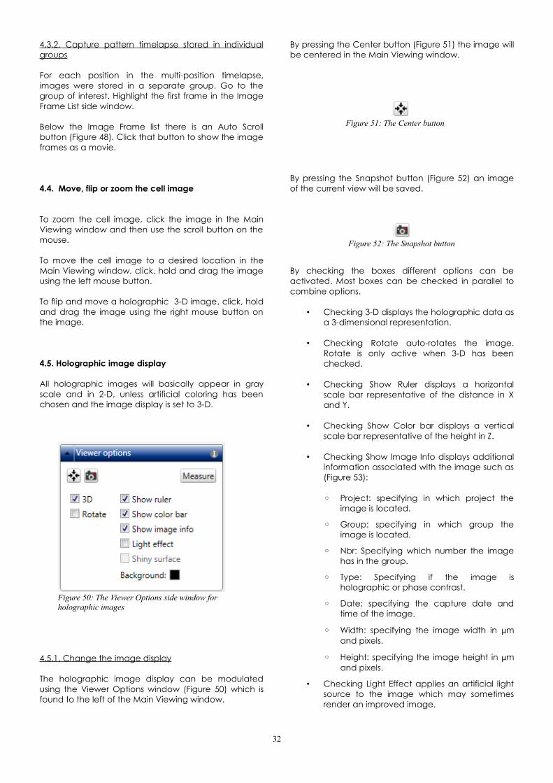
The holographic image display can be modulatedusing the Viewer Options window (Figure 50) which isfound to the left of the Main Viewing window.

By pressing the Center button (Figure 51) the image willbe centered in the Main Viewing window.

By pressing the Snapshot button (Figure 52) an imageof the current view will be saved.

By checking the boxes different options can beactivated. Most boxes can be checked in parallel tocombine options.

• Checking 3-D displays the holographic data asa 3-dimensional representation.

• Checking Rotate auto-rotates the image.Rotate is only active when 3-D has beenchecked.


• Checking Show Color bar displays a verticalscale bar representative of the height in Z.

• Checking Show Image Info displays additionalinformation associated with the image such as(Figure 53):

◦ Project: specifying in which project theimage is located.

◦ Group: specifying in which group theimage is located.

◦ Nbr: Specifying which number the imagehas in the group.

◦ Type: Specifying if the image isholographic or phase contrast.

◦ Date: specifying the capture date andtime of the image.

◦ Width: specifying the image width in μmand pixels.

◦ Height: specifying the image height in μmand pixels.


32

Figure 50: The Viewer Options side window for holographic images

Figure 51: The Center button


• Checking Shiny surface applies a change inthe surface image display that sometimesrenders a better image. Shiny surface is onlyactive when Light Effect is checked.

4.5.2.Change the image coloring

All holographic images will appear in gray scale. Usethe Coloring side window (Figure 54), which is found tothe left of the Main Viewing window, to add artificialcoloring to the images. The colors that are applied willbe distributed in the image relatively to the thicknessof the objects.

A set of colors that are saved together is called acolorset. A previously saved colorset can be used withthe current image by making a selection in theColorset list which is found at the top of the Coloringside window (Figure 54).

• By left clicking the R-button (Figure 55) thecoloring in the image is rescaled to betterutilize the optimal dynamic range of theimage. This button needs to be operatedevery time the image coloring is off.

• To add a new color, left click the plus-button(Figure 55) and click Add Color. Select a color.A colored triangle representing the new colorwill appear beneath the histogram (Figure 54).Alternatively, right click on the X-axis andselect Add Color.

• Change the color by using the right mousebutton to click on a colored triangle beneaththe histogram (Figure 54)and select a newcolor. Alternatively left click the arrow button(Figure 55) and select Change Color.

• To change the color span, left click and movethe desired colored triangle beneath thehistogram (Figure 54) using the cursor. To savethe current color settings to a new colorset, leftclick the arrow button and choose Save As(Figure 55).

• To save the current color settings to an alreadyexisting colorset, left click the arrow buttonand click save (Figure 55). Note that this willoverwrite the settings previously saved to thiscolorset.

• To delete a colorset, select it in the Colorset list.Then left click the arrow button (Figure 55) andclick Delete Colorset.

• To save a colorset to an image, left click thearrow button (Figure 55) and choose Apply Tofollowed by Frame. The current colorset will beapplied to the currently viewed frame andsaved.

• To save several images with the currentcolorset, check the box of the desired imagesin the Image Frame List side window (Figure46), left click on the arrow button in theHistogram side window (Figure 55). ChooseApply To followed by left clicking CheckedFrames. The current colorset will be applied tothe checked image frames and saved.

33

Figure 55: Additional functions found in the Coloring side window

Figure 53: Hologram Image Information


Note that changes regarding color will not in any wayaffect the raw data, and that the original gray-scaleimage always can be retrieved.

4.6. Move, flip or zoom the cell image

To zoom the cell image, click the image in the MainViewing window and then use the scroll button on themouse.

To move the cell image to a desired location in theMain Viewing window, click, hold and drag the imageusing the left mouse button.

To flip and move a holographic 3-D image, click, holdand drag the image using the right mouse button onthe image.

4.7. Recalculate a holographic image

If a holographic image is not correctly focused, as inthis example (Figure 56), the software focus can berecalculated after capture in the View Images tab bychanging the software calculation settings.

4.7.2. Recalculate the focus manually

After image capture most images are well focused.Some cell samples are more demanding and need tobe adjusted manually. Check Manual in the SoftwareFocus side window (Figure 57).

The text box next to the Manual button shows thesoftware focus distance in mm. The distance can bechanged either by entering a value manually or byusing the slide bar beneath the text box.

To determine which focal distance that will result in awell focused image is often a matter of trial and error.To find a starting value, choose an image that wascaptured at the same time and that is well focusedand note the focal distance of that image.

Highlight the image that needs to be recalculated.Select Manual in the Software Focus side window andenter the focal distance of the well focused image inthe text box.

Click Update.

If the image focus needs to be improved, enter a newfocal distance and click Update. Continue until theimage is well focused.

Use the arrow button to apply the update to either thecurrent frame or to all checked frames.

4.7.1. Recalculate the focus automatically

To replace the manual changes with the originalcomputer focus, Select Automatic in the SoftwareFocus side window (Figure 58) and then click theUpdate button.

If the result is a well focused image, use the arrowbutton to apply the update to either the current frameor to all checked frames.

34

Figure 56: An unfocused holographic image

Figure 57: The Calculation Settings side window set to manual

Figure 58. The Calculation Settings side window set to automatic

4.7.3. Recalibrate a holographic image

If a captured or imported image is not correctlycentered due to aberrant calibration of the instrument,the image will look strange (Figure 59). It can be re-calibrated. Clicking the Recalibrate button (Figure 60)in the Software Focus side window will result in a re-centered image with an adjusted focal distance(Figure 61).

4.7.4 Using a background hologram

The images are noise-improved by using a backgroundhologram to subtract noise from the image. If thebackground hologram is not correctly set, it mightinstead disturb the image calculations. There is anoption not to use the background hologram (Figure60).

35

Figure 60: The More list with the Recalibration button and the Use Background Hologram function in the Calculation settings side window

Figure 59: Example of an incorrectly calibrated image

Figure 61: An example of a recalibrated image

Chapter 5. Cell identification

The base for all image analysis is the cell identification.The software has already made a segmentationsuggestion, which might be very good, but it mightalso need adjustments.

The cell number and confluence of each image isimmediately given beside the image in the ImageFrame List window (Figure 63).

Note that the software will suggest a cell identificationat the time of capture. This automatic identificationneeds to be evaluated for each image.

5.1. Identify cells

Choose the Identify Cells tab (Figure 62).

5.1.1. Select an image

The Image Frame List side window (Figure 63) is foundto the right of the Main Viewing window (Figure 5).Select the project and group where the images aresaved (Figure 63). Highlight the image of interest tomake it appear in the Main Viewing Window.

5.1.2. Automatic threshold settings

The software will automatically make threshold settingsaccording to the default segmentation method (Figure64).

There are several other methods to calculate thethreshold settings in the Methods list in the Adjustmentswindow (Figure 65) which is found below the MainViewing window.

The different threshold settings calculation methods(Figure 65) will result in slightly different cellidentifications. It is advisable to try out which methodthat works best for every type of cell sample.

• Manual allows the user to set the globalthreshold level using the slider.

• Minimum error sets the global threshold level

36

Figure 62: The Identify Cells tab

Figure 64: Identified cells

Figure 63: The Frame List side window

Figure 65: The Adjustments tab showing the different methods to calculate threshold settings

using the minimum error histogram-basedthreshold method.

• Otsu sets the global threshold level using theOtsu method.

• Otsu in blocks: the image is split into blockswhich are thresholded separately using Otsumethod. This is a form of adaptive threshold.

• Adaptive mean sets an adaptive thresholdingusing a mean filter.

• Adaptive gaussian sets an adaptivethresholding using a gaussian filter.

• Double otsu: double thresholding is a methodwhere both a wide and a narrow thresholdmask is used. The narrow image ismorphologically reconstructed under the wideimage. The final image is used as thresholdmask. The result is a cleaner threshold mask.The Double Otsu uses double thresholding withOtsu global threshold as mid level threshold.

• Double adaptive mean: same as Double Otsubut with two adaptive mean threshold masks.

• Double adaptive gaussian: same as DoubleOtsu but with two adaptive gaussian thresholdmasks.

5.1.3. Adjust the cell identification

In the Adjustments window, which is found below theMain Viewing window (Figure 66), the cell identificationsettings can be adjusted in several ways. In addition toselecting the method to calculate the threshold, asdescribed above, adjustments can be made for eachmethod.

The slide bar labeled Adjustment (Figure 66) is used tomanually adjust the threshold that is set between cellsand background, thus adjusting the area of thesegmented cells.

The slide bar labeled Minimum Object Size (Figure 66) isused to manually adjust the size of the cell core, thusadjusting which identified areas that are cells.

• Checking Presmoothing (Figure 66) activates anoise reduction function that will smooth theedges of the cells.

• Checking Join Nearby Markers (Figure 66)results in two distinct cell markers beingcounted as one when they are very close toeach other.

5.2. Make adjustments for single cells

It is possible to make manual changes to the cellidentification for individual cells. It is possible to add,remove and delete as well as enlarge or shrinkidentified cells. These functions are found in theManual Changes window (Figure 67) below the MainViewing window.

• Add or Remove (Figure 67) allows the user toadd or remove the blue cell markers thatidentify the cell core. This results in mergers orsplits of identified cell areas.

• Grow or Shrink allows the user to enlarge orshrink the identified cell regions.

• Delete Area allows the user to removeidentified cell areas.

37

Figure 66: The Adjustments window

Figure 67: The Manual Changes window

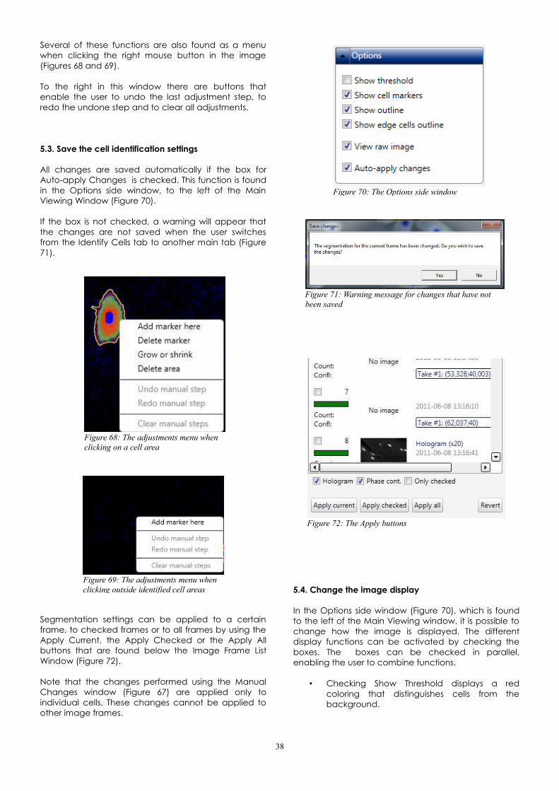
Several of these functions are also found as a menuwhen clicking the right mouse button in the image(Figures 68 and 69).

To the right in this window there are buttons thatenable the user to undo the last adjustment step, toredo the undone step and to clear all adjustments.

5.3. Save the cell identification settings

All changes are saved automatically if the box forAuto-apply Changes is checked. This function is foundin the Options side window, to the left of the MainViewing Window (Figure 70).

If the box is not checked, a warning will appear thatthe changes are not saved when the user switchesfrom the Identify Cells tab to another main tab (Figure71).

Segmentation settings can be applied to a certainframe, to checked frames or to all frames by using theApply Current, the Apply Checked or the Apply Allbuttons that are found below the Image Frame ListWindow (Figure 72).

Note that the changes performed using the ManualChanges window (Figure 67) are applied only toindividual cells. These changes cannot be applied toother image frames.

5.4. Change the image display

In the Options side window (Figure 70), which is foundto the left of the Main Viewing window, it is possible tochange how the image is displayed. The differentdisplay functions can be activated by checking theboxes. The boxes can be checked in parallel,enabling the user to combine functions.

• Checking Show Threshold displays a redcoloring that distinguishes cells from thebackground.

38

Figure 72: The Apply buttons

Figure 71: Warning message for changes that have not been saved

Figure 70: The Options side window

Figure 68: The adjustments menu when clicking on a cell area

Figure 69: The adjustments menu when clicking outside identified cell areas

• Checking Show Cell Markers displays a bluecoloring that indicates the cell core.

• Checking Show Outline displays yellow linesthat indicate the border of the cells.

• Checking Show Edge Cells Outline displaysyellow lines that indicates the border of thecells touching the image edges.

• Checking Raw Image causes the image to bedisplayed as the unadulterated gray scaleimage

• Using Auto-apply Changes allows the user toimplement all changes immediately.

5.5. Image information

When the mouse cursor hovers over one of thesegmented cells, information concerning that cell willbe displayed (Figure 73).

• Area is the cell area in m2.

• Volume is the optical cell volume in m3. Thevolume measurements are based on thephase shift of the light and are thereforecalled “optical”.

• Thickness max is the optical thickness of thecell is at its thickest in m.

• Thickness avg is the average optical thicknessof the cell in m.

• Perimeter length is the circumference of thecell in m.

• Eccentricity is how elongated the cell is or inhow much the cell deviates from being acircle, with 0 corresponding to the perfectcircle and 1 being the maximum eccentricity.

• Irregularity is how much the circumference ofthe cell deviates from the circumference of aperfect circle with 0 corresponding to theperfect circumference and 1 being themaximum deviation.

39

Figure 73: Information pertaining to a single identified cell

Chapter 6. Cell Tracking

Cells can be tracked through a timelapse sequenceand analyzed both for movement and for morphologychanges over time.

6.1. Start tracking cell movement

Go to the Cell Tracking tab (Fig 74). A window willappear where a new analysis or a stored analysis canbe selected (Figure 75).

After clicking the New Analysis button a text willappear which says that frames must be added in orderto analyze images for cell tracking (Figure76).

6.1.1 Add image frames to the analysis

Highlight or check the images to be analyzed, in theImage Frame List to the right. Click the appropriateAdd button (Figure 77). The Add buttons are foundbelow the Image Frame List. The added image frameswill be shown in the Source Frames window (Figure 78)below the Cell Tracking window (Figure 91).

6.1.2. Select cells to be analyzed

In order to follow a cell through a timelapse, the cellneeds to be added. Go to the Select Mode sidewindow (Figure 79), and activate Add Cells.

In the Cell Tracking window, the center of eachidentified cell is marked with a small orange + (Figure80). If the identification is not satisfying, go to theIdentify Cells tab, and adjust the cell identification(Chapter 5). Click each cell to be followed (Figure 80).The cell will be followed from the frame where it isadded.

6.1.3. Displaying the cell tracking

There is a Timeline below the Cell Tracking window(Figure 81). By moving the small gray slider, the imageframe sequence will be played through. The tracksshowing the cell movements movement will then bedisplayed (Figure 82).

40

Figure 74: The Cell Tracking tab

Figure 76: The Cell Tracking instruction text

Figure 78: The Source Frames window

Figure 77: The Add buttons

Figure 79: The Select Mode sidewindow

Figure 80: Clicking to add a cell to the tracking results

Figure 75: The Select Analysis buttons

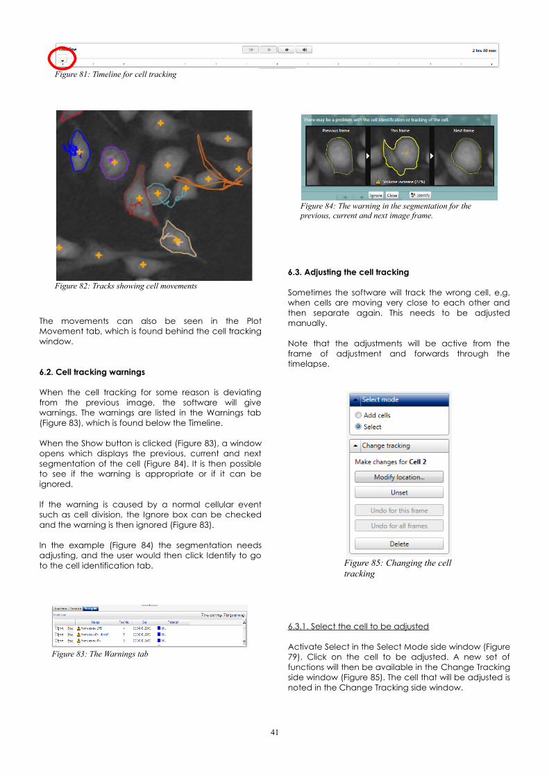
The movements can also be seen in the PlotMovement tab, which is found behind the cell trackingwindow.

6.2. Cell tracking warnings

When the cell tracking for some reason is deviatingfrom the previous image, the software will givewarnings. The warnings are listed in the Warnings tab(Figure 83), which is found below the Timeline.

When the Show button is clicked (Figure 83), a windowopens which displays the previous, current and nextsegmentation of the cell (Figure 84). It is then possibleto see if the warning is appropriate or if it can beignored.

If the warning is caused by a normal cellular eventsuch as cell division, the Ignore box can be checkedand the warning is then ignored (Figure 83).

In the example (Figure 84) the segmentation needsadjusting, and the user would then click Identify to goto the cell identification tab.

6.3. Adjusting the cell tracking

Sometimes the software will track the wrong cell, e.g.when cells are moving very close to each other andthen separate again. This needs to be adjustedmanually.

Note that the adjustments will be active from theframe of adjustment and forwards through thetimelapse.

6.3.1. Select the cell to be adjusted

Activate Select in the Select Mode side window (Figure79). Click on the cell to be adjusted. A new set offunctions will then be available in the Change Trackingside window (Figure 85). The cell that will be adjusted isnoted in the Change Tracking side window.

41

Figure 81: Timeline for cell tracking

Figure 82: Tracks showing cell movements

Figure 83: The Warnings tab

Figure 84: The warning in the segmentation for the previous, current and next image frame.

Figure 85: Changing the celltracking

6.3.2. Switch the tracking from one cell to another

After selecting the cell to be changed, click the ModifyLocation button in the Change Tracking side window.Then click the cell that actually should be followedinstead of the selected cell. Now, the colored border istransferred to the new cell to be followed (Figure 86).The software will recalculate the trackingautomatically from the present image frame andforward through the time lapse.

6.3.3. Discontinue a cell tracking

Sometimes a tracking needs to be discontinued, e.g.when a cell leaves the image area.

After selecting the cell to be changed, click the Unsetbutton in the Change Tracking side window (Figure ).The tracking will be discontinued from the presentframe.

A new button, Set location, will appear in the ChangeTracking window (Figure 87).

6.3.4. Continue a discontinued cell tracking

When a cell has been unset it will still be present in theTracked Cells list, but noted as not present. In order toresume the tracking in a different frame, select the cellin the Tracked Cells list and click the Set locationbutton (Figure 87). Then click the cell in the framewhere the tracking should be resumed.

6.3.5. Undo manual changes

If the manual changes need to be undone, start byselecting a cell. Then click either the Undo for thisFrame, or the Undo for all Frames button (Figure 85).

When clicking Undo for this Frame, the manual changein the current frame will be undone, and the trackingwill be recalculated according to the change insettings.

When clicking Undo for all Frames, the manualchanges in all frames will be removed and the trackingwill be recalculated according to the change insettings.

6.4. Tracking cell morphology

Once the cell movement has been tracked, the cellmorphology can also be followed over time by usingthe Plot Features tab (Figure 88).

6.4.1 Display cell morphology parameters for individualcells

By checking or unchecking the colored boxesdisplayed beside each cell name, morphologicalparameters are shown for that cell. Black always showsthe average of the cell population.

6.4.2 Display different cell morphology parameters

By using the Cell Feature function found below thediagram (Figure 89) different morphologicalparameters can be displayed. The list contains allparameters as well as distance and speed ofmovement. For a full list of parameters, go toAddendum A.

42

Figure 86: Transfer the tracking from one cell to another. The left image shows the selected cells, and the right image shows how the tracking is transferred.

Figure 87: Set Location

Figure 88: The Cell Morphology Tracking tab

Figure 89: Switching cell features

6.5. Export the tracking results

The raw data can be exported into an xml-file byclicking the Export button (Figure 104) which is found inthe Tracking tab. The xml-file can be imported into e.g.Xcel.

The image currently displayed in the cell trackingwindow can be saved by clicking the Save button,found below the Cell Tracking window (Figure 91),which is found in the Tracking tab.

43

Figure 91: The Save button which is found below the Cell Tracking window

Figure 90: Track and Export buttons found to the right of the Cell Tracking window in the Tracking tab

Chapter 7. Analyze and export data

The main part of the cell data analysis is performed inthe Analyze Data tab that contains tools for analyzingthe identified cells.

A simple tool for measuring distances or objects in acurrently viewed image is found in the View Imagestab.

7.1. Measure distances directly in the currently viewedimage

Choose the View Images tab (Figure 92).

Click the Measure button in the Viewer Options sidewindow (Figure 93) to make manual measurements ofobjects in the current image.When the measuring function is activated, themeasurement is started by left clicking anywhere inthe image. The measurement is finished by left clickingat a new point in the image.

The measured distance is shown with a blue bar (Figure94). A window displaying the results appear to thebottom right of the main viewing window. The resultsinclude a profile of the measured object.

The data are saved as an image when the Snapshotbutton (Figure 95) in the Viewer Options window isclicked.

It is possible to move the image in the Main Viewingwindow while the measuring function is activated. Theimage is moved by clicking and dragging.

When the Measure button is clicked again, themeasuring function is deactivated.

7.2. Analyze results in plot

7.2.1. Start a new analysis

Choose the Analyze Data tab (Figure 96).

A window will appear where a new analysis or a storedanalysis can be selected (Figure 97).

After clicking the New Analysis button a new messagewill appear (Figure 98).

44

Figure 96: The analyze data tab

Figure 94: The blue measuring bar and the results window

Figure 92: The View Images tab

Figure 93: The Viewer Options side window for holographic images

Figure 97: The Select Analysis buttons


Select a Project and a Group in the Image Frame listwindow (Figure 99), which is found to the right of theMain Viewing window (Figure 5).

To add data, highlight image/s and transfer to the plotby using the Add Selected button (Figure 100), which isfound below the Image Frame list window. Severalimages can be added simultaneously if they are allhighlighted. The shift key can be used to highlightseveral consecutive images and the ctrl key tohighlight non-consecutive images.

The images that are included in the analysis are shownin the Source Frames tab (Figure 101) which is foundbelow the Main Viewing window.

If several images are added to the plot, the data fromall images will be displayed in the same plot unless theOnly Current Frame (Figure 102) is checked. Then onlythe data from the current frame are displayed. TheOnly Current Frame function is found below theScatter-plot.

7.2.2. Remove data from plot

To remove data belonging to a single frame from aplot, highlight that frame in the Source Frames list(Figure 101). Then use the remove button that is foundabove and to the right of the Source Frames list(Figures 101 and 103).

7.3. Display results in scatter-plot

The cell morphology data are first represented as ascatter-plot, with the segmented cell images displayedbeside the plot (Figure Fel: Det gick inte att hittareferenskällan). The data point for each cell isrepresented as a colored box. If several frames arerepresented in the plot, the data points from all imageswill be displayed in the plot simultaneously, while thecell image window shows the frame that is highlightedin the Source Frames tab.

The data points will be displayed in the plot with thecolor shown in the color box in the Source Frames tab(Figure 105), which is found below the Scatter-plot tab.To change the display color, left-click the color box forthe added frame and select a different color.

45

Figure 100: The Add buttons below the Image Frame list

Figure 102: The Only Current Frames function

Figure 101: The Source Frames tab which is found below the Scatter-plot tab

Figure 103: The Remove from Plot buttons

Figure 99: The Image Frame list

Figure 98: The Add message

7.3.1. Identify data points as cells

Hover with the mouse cursor over a data point in thescatter-plot. The corresponding cell will then beidentified in one of the cell images that have beenadded to the plot (Figure 106). Data for that cell will bedisplayed simultaneously.

When hovering over a certain cell in an added imageframe, the data point representing that cell will beidentified in the scatter-plot, and data for that cell willbe displayed (Figure 107).

46

Figure 105: The several plot display colors that can be selected

Figure 106: Identifying the cell represented by a certain data point

Figure 107: Identifying the data point representing a certaincell

Figure 108: The X- and Y-axis labels

Figure 104: Results displayed in a scatter plot shown with the corresponding image frame

7.3.2. Change the scatter-plot axis units

The axis labels of the scatter-plot can be changed byusing the listed X- and Y-axis parameters found belowthe scatter plot (Figure 108). For a full list of axis labelparameters, go to Addendum A.

7.3.3. Change the scatter-plot axis display manually

The Plot Area settings (Figure 109) are found below theScatter-plot. The area of the scatter-plot (i.e. thevalues of the X- and Y-axis) is set automatically to fit inall values from all added frames.

To set the plot area manually, deactivate Auto-scaleby unchecking the box (Figure 109) and then enteringthe desired X and Y minimum and maximum values(Figure 110).

Alternatively, the plot area can be changed with themouse scroll button. Left click in the plot and scrollusing the mouse scroll button.

To move the plot area in the scatter-plot, left click inthe plot, hold and drag.

7.3.4. Create, hide and delete plot regions

The scatter-plot diagram can be divided into regionsto separate out data from certain cells or cellpopulations. When clicking the right mouse buttonwhile hovering over the plot, a menu will open. WhenDefine New Region is selected, a region menu willappear (Figure 112). Alternatively there is an DefineRegion button (Figure 111) below the Scatter-plot tab,to the right of the Auto-scale function.

In both cases a list of region types appears (Figure112). Select a region type by clicking it. Then click inthe plot where the region setting should begin.

For the linear region and the X- and Y- axis regions thesecond click in the plot determines where the regionends.

For the arbitrary region, every click in the plot will addto the region. Finish the region by clicking the startingpoint again. The starting point will expand to indicatethat the region is closed. If clicking the region does notmake it “stick”, try clicking a little slower.

• X-axis region, where X-axis values are theregion cut off values (Figure 113).

• Y-axis region, where Y-axis values are theregion cut off values (Figure 113).

• Linear region, where clicking in the diagramwindow results in straight lines that cut off theregion from origin (Figure 114).

• Arbitrary region, where repeated clicking inthe diagram window results in an irregularfigure that outlines the region. To finish theregion, close it off by clicking in the startingpoint (Figure 114).

The regions are summarized in the Regions tab (Figure115), which is found below the Scatter-plot tab.Regions can be hidden by unchecking the Displaybox.

Regions can be deleted by highlighting the region inthe Regions window and then clicking Delete, which isfound to the upper right in the regions tab (Figure 116).

47

Figure 110: The Fixed Plot Area window

Figure 112: A list of region types

Figure 111: The Define Region button

Figure 109: The Plot Area settings

7.4. Display results in histograms

The results can also be displayed as histograms, whereone cell parameter is offset against the cell number(Figures 117 and 118).

When Only Current Frame (Figure 119) is checked, thedata from each frame is displayed when thecorresponding image is highlighted in the SourceFrames tab (Figure 120) below the Scatter Plot tab.

The data from each image frame will be representedin the histogram with the color shown in the color boxin the Added Frames window.

To change the display color, left-click the color boxbeside the frame number in the Source Frames taband select a different color (Figure 121).

48

Figure 115: The Regions tab

Figure 113: An X-axis region (green) and a Y-axis region (blue)

Figure 114: A linear region (blue) and an arbitrary region(green)

Figure 117. The Histogram tab

Figure 119: The Only Current Frame button

Figure 116: The Delete buttons

Figure 118. A Histogram

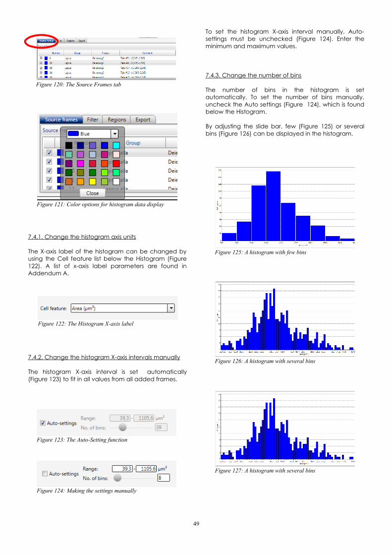
7.4.1. Change the histogram axis units

The X-axis label of the histogram can be changed byusing the Cell feature list below the Histogram (Figure122). A list of x-axis label parameters are found inAddendum A.

7.4.2. Change the histogram X-axis intervals manually

The histogram X-axis interval is set automatically(Figure 123) to fit in all values from all added frames.

To set the histogram X-axis interval manually, Auto-settings must be unchecked (Figure 124). Enter theminimum and maximum values.

7.4.3. Change the number of bins

The number of bins in the histogram is setautomatically. To set the number of bins manually,uncheck the Auto settings (Figure 124), which is foundbelow the Histogram.

By adjusting the slide bar, few (Figure 125) or severalbins (Figure 126) can be displayed in the histogram.

49

Figure 122: The Histogram X-axis label

Figure 125: A histogram with few bins

Figure 126: A histogram with several bins

Figure 120: The Source Frames tab

Figure 121: Color options for histogram data display

Figure 124: Making the settings manually

Figure 127: A histogram with several bins

Figure 123: The Auto-Setting function

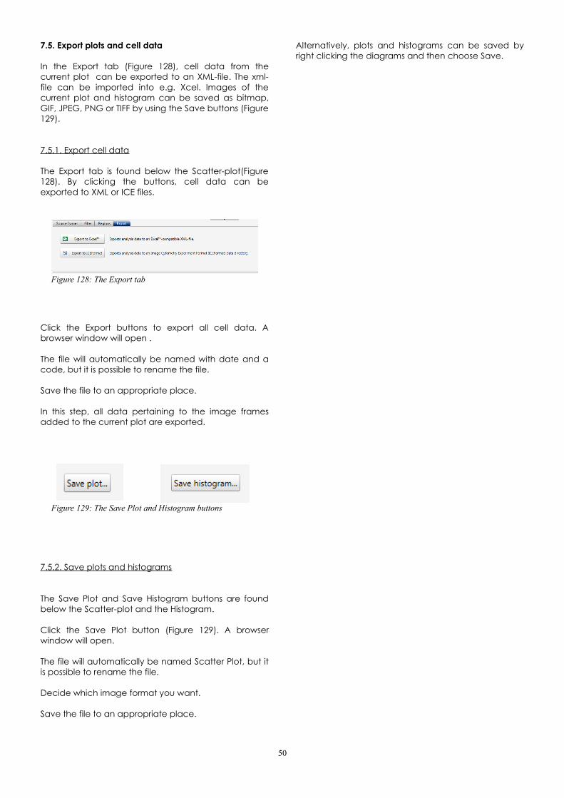
7.5. Export plots and cell data

In the Export tab (Figure 128), cell data from thecurrent plot can be exported to an XML-file. The xml-file can be imported into e.g. Xcel. Images of thecurrent plot and histogram can be saved as bitmap,GIF, JPEG, PNG or TIFF by using the Save buttons (Figure129).

7.5.1. Export cell data

The Export tab is found below the Scatter-plot(Figure128). By clicking the buttons, cell data can beexported to XML or ICE files.

Click the Export buttons to export all cell data. Abrowser window will open .

The file will automatically be named with date and acode, but it is possible to rename the file.

Save the file to an appropriate place.

In this step, all data pertaining to the image framesadded to the current plot are exported.

7.5.2. Save plots and histograms

The Save Plot and Save Histogram buttons are foundbelow the Scatter-plot and the Histogram.

Click the Save Plot button (Figure 129). A browserwindow will open.

The file will automatically be named Scatter Plot, but itis possible to rename the file.

Decide which image format you want.

Save the file to an appropriate place.

Alternatively, plots and histograms can be saved byright clicking the diagrams and then choose Save.

50

Figure 128: The Export tab

Figure 129: The Save Plot and Histogram buttons

Chapter 8. Cell Count

Cells are counted and analyzed for confluence, cellarea and volume in the Cell Count tab.

8.1. Count cells

Choose the Cell Count tab (Figure 130).

A text will appear which says that five image frames ormore must be added in order to analyze images forcell count, confluence, cell area and volume (Figure131).

Highlight or check the images to be analyzed, in theImage Frame List to the right. Click the appropriateAdd button (Figure 132). The Add buttons are foundbelow the Image Frame List. The added image frameswill be shown in the Source Frames window below theCell Count Report (Figure 133).

Fill in the correct cell culture vessel growth area andthe volume of the cell culture vessel medium contentin the text boxes below the Cell Count Report (Figure134).

The images are then analyzed, and the results arepresented in a Cell Count Report (Figure 135).

The report contains data on:

• Number of cells in the vessel.

• Number of cells per ml.

• Confluence.

• Report date.

• Capture time points.

• Vessel growth area.

• Vessel media volume.

• Total number of image frames used for theanalysis.

• The total area of the images.

• The total number of cells in the images.

• The number of cells that are placed on theimage edge, and which therefore are notincluded in the morphological analysis,although they are included in the cell count.Of the edge cells 50% are included in the thecell number while 50% are not included.

If the confidence interval is too large (larger than 10-15%) more images should be added to the analysis.The more unevenly the cells grow, the more imagesare needed for the cell count.

51

Figure 131: The Cell Count instruction text

Figure 132: The Add buttons

Figure 135: The Cell Count Report

Figure 133: The Source Frames window

Figure 130: The Cell Count tab

Figure 134: Text boxes for cell culture vessel area and volume

8.2. Adjust the histogram proportions

The X-axis of the Area and Volume histograms can beset either automatically, or manually. For each axis thelowest and the highest value can be set as well as thenumber of bins that present the data.The adjustment text boxes are found below the cellcount report window (Fig. 136).

8.3. Remove data from plot

To clear the plot from all data from all image frames,use the Remove All command, which is found with anX to the right in the Source Frames window (Figure 137).

To remove data belonging to a single frame from aplot, highlight that frame in the Source Frames windowand then use the Remove Highlighted command,which is found with an X to the right in the SourceFrames window (Figure 137).

8.4. Export results

Below the Cell Count Report there is a Save reportbutton (Figure 138). Clicking the button generates apdf containing all relevant data, including the areaand volume as histograms and a list of the includedimage frames. When the boxes are un-checked,histograms and frame list can be excluded from thereport.

52

Figure 137: The Remove functions

Figure 138: The Save Report button

Figure 136: The histogram adjustment functions

Chapter 9. Export images and movies

In the Export Images tab, image frames can be editedand exported either as individual images in severalstandard formats or as AVI movies (Figure 139).

9.1. Add and remove image frames

Below the Image Frame list (Figure 140) there arebuttons to add image frames to the Main Window. Theside windows become active only when one or severalimages have been added.

By clicking the Add Highlighted button (Figure 140)which is found below the Image Frame list, the datafrom a single image frame or from several frames canbe added when the frames are highlighted in theImage Frame list. The shift key can be used to highlightseveral consecutive images and the ctrl key tohighlight non-consecutive images.

Alternatively, the box to the left of each image can bechecked and then the Add Checked button is clicked.

All image frames can be added by clicking the Add Allbutton.

Clicking the Remove buttons (Figure 141) will removeeither only the highlighted or all of the added images.

The Main Viewing Window contains a view of thecurrently active added image as well as thumb nails ofall the added images (Figure 142). By clicking a thumbnail a new image will be displayed in the Main Viewingwindow.

53

Figure 140: The Image Frame list

Figure 142: The Main Viewing window

Figure 139: The Export Images tab

Figure 141: The Remove buttons

9.2. Edit the images

9.2.1. Zoom, move or flip the image

The Perspective side window (Figure 143) shows howthe image has beenmoved, flipped or zoomed.

To zoom, left click the cell image in the Main Viewingwindow and then use the mouse scroll button.

To move the image to a desired location in the MainViewing window, click, hold and drag using the leftmouse button.

To flip and move the 3-D image, click, hold and dragusing the right mouse button.

Click one of the Use-buttons to apply the changes tothe added images that are highlighted or to all addedimages.

9.2.2. Adjust the image display

The Viewer Options side window (Figure 144), which isfound to the left of the Main Viewing window, is usedto adjust the image display. Some of the options areinactive when a phase contrast image is viewed.

• Checking 3-D displays the image as a 3-dimensional representation.


• Checking Show Color Bar displays a verticalscale bar representative of the height in Z.

• Checking Show Image Info displays additionalinformation associated with the image suchas:

◦ First row: specifies in which project theimage is located.

◦ Second row: specifies in which group theimage is located.

◦ Nbr: specifies which number the imagehas in the group.

◦ Type: specifies if the image is holographicor phase contrast.

◦ Date: specifies the capture date and timeof the image.


54

Figure 143: The Perspective side window

Figure 145: The Background color setting

Figure 144: Viewer Options side window

• Checking Shiny surface applies a change inthe surface image display that sometimesrenders a better image. Shiny surface is onlyactive when Light Effect is checked.

• To change the Background color, left click theBackground color box and select a new color(Figure 145).

9.2.3. Holographic image coloring

Adjust the holographic image color display and theimage dynamics with the Coloring side window (Figure146).

A set of colors that are saved together is called acolorset. A previously saved colorset can be used withthe current image by making a selection in theColorset list which is found at the top of the Coloringside window (Figure 146).

Click one of the Use-buttons to apply the changes tothe added images that are highlighted or to all addedimages.

Additional functions are found as buttons and in amenu which is found at the arrow tip (Figure147).

• By left clicking the R-button (Figure 147) thecoloring in the image is rescaled to betterutilize the optimal dynamic range of theimage. Note that this button needs to beoperated every time the image coloring is off.

• To add a new color to the colorset, left clickthe plus button (Figure 147) and select a new

color. A colored triangle representing the newcolor will appear beneath the histogram(Figure 146). Alternatively, right click the x-axisat the position where a new color is wantedand select Add Color from the menu thatappears.

• Change the color by using the right mousebutton to click on a colored triangle beneaththe histogram and select a new color,alternatively left click the arrow button andselect Change Color (Figures 146 and 147).

• To change the color span, left click and movethe desired colored triangle beneath thehistogram using the cursor (Figure 146).

• To save a new colorset with the current colorsettings, left click the arrow button and chooseSave As (Figure 147).

• To save the current color settings to apreviously saved colorset, left click the arrowbutton and choose Save (Figure 147). Notethat this will overwrite the settings previouslysaved to this colorset.

9.3. Create an AVI movie

When the set of images look good, click the Use ForAll-buttons in both the Perspective side window andthe Coloring side window (Figures 143 and 146).Preview the movie by clicking the preview button Play(Figure 148). The number of slides per second are notshown as in the finished movie, but rather at a setspeed.

55

Figure 147: Additional functions foundin the Coloring side window


If the preview looks good, click the Export Moviebutton in the Export window (Figure 149).

Clicking the Export Movie button will open an exportwindow (Figure 150). Select the destination folder bybrowsing. By moving the slide bar it is possible to set thenumber of frames per second that will be shown in theAVI movie.

9.4. Export images

When the image has been set up nicely and looksgood, click the Export Images button to open anexport window (Figure 151). Select the destinationfolder by browsing. Check the box to add framecomments to the file name. The Image format can beselected in the drop menu.

When the box for Use Plain Image Images is checked,no coloring or 3-D will be displayed in the exportedimage.

When the box for Transparent Background is checked,the images will be exported without background.

56

Figure 148: The Preview side window

Figure 149: The Export window

Figure 150: The Export Movie side window

Figure 151: The Export Images side window

Chapter 10. Back up

In order to make a safety back up of your data youneed to either export or copy the database.

10.1. Back up of individual projects, groups or frames

Click Database in the top menu (Figure 152). Then clickExport.

A browser window will open (Figure 153). Click Browse.Create a new folder at the selected destination (Figure154).

When a folder has been created, a window displayingthe groups and projects will appear (Figure 155). Selectthe projects, groups or images that you want toexport/back up.

Click Export. Alla database information will now becopied to the created folder.In order to access the data in the folder, the data mustbe imported into the software again using DatabaseImport.

10.2. Back up of the entire database

First locate the database. Click Database in the topmenu (Figure 152). Then click Settings. Determine theRoot Directory for the database folderHstudioimageDB (Figure 156).

57

Figure 152: The Database menu

Figure 153: The Browser window

Figure 154: Create new folder

Figure 155: Select projects, groups or images for export

Figure 156: Database settings information containing the root directory of HstudioimageDB

Find HstudioimageDB on the computer hard drive(Figures 157 and 158). Note that the root directory isdifferent for different computers.

Copy the entire HstudioimageDB folder. In order toaccess the data in the folder, HoloStudio must bedirected to use the copied data base.

58

Figure 158: The PHI folder that contains the HstudioimageDB database

Figure 157: The pathway to the PHI folder

Chapter 11. Troubleshooting

11.1. Live Imaging

11.1.1. The Live Capture tab is inactive

Why? The software cannot find the HoloMonitor.Fix: Check that the USB- and power cables areproperly connected. Try restarting HoloStudio.

Why? The drivers are corrupt.Fix: Start the Windows Device Manager and check forany drivers with exclamation marks. Try disconnectingthe USB-cable from the instrument and connect itagain and wait a couple of minutes. If the problempersists, try to run the installation program again. Thedriver files are located under C:\PHI\Drivers assubfolders. If a driver has an exclamation mark shownin device manager it may be possible to re-install it byright-clicking in device manager and selecting Updatedriver. Then browse to driver folder underC:\PHI\Drivers.

11.1.2. It is impossible to focus the live image

Why? For M4 with distance plates, the wrong distanceplate might be used. Fix: Make sure that the correct spacer plate or vesselholder for that cell culture vessel is used. The bottom ofthe vessel (where the cells are) should beapproximately 1 mm from the objective. Vessels with athick bottom or a high socket need the thinnest spacerplate. Vessels or slides which are thin should be put onthe thickest or medium thick distance plate.

Why? The cell culture vial is scratched or smudged. Fix: Even wiping the cell culture vessel clean willprobably not help much as traces of dirt will still persist.Instead, avoid touching the top and bottom surfacesof the cell culture vessel when handling it, even whenwearing gloves. Avoid anything that might scratch thesurfaces. Cell culture plastic is very easily scratched.

Why? There is condensation on the inside of the cellculture vessel.Fix 1: If the cell culture vessel is a flask, tighten the capand gently rinse the condensation away with the cellculture medium. Avoid getting medium into the cap. Ifthe cell culture vessel is a multiwell plate or a petri dish,allow the vessel to reach room temperature,alternatively switch lids to a new lid or try workingwithout a lid. NOTE! Working without the lid is a non-sterile procedure! Fix 2: If the cell culture medium is replaced with coldPBS or cold cell culture medium immediately aftertaking the multi well plates and petri dishes from theincubator, there will not be condensation. Replace thePBS with medium again after the analysis.

Why? The laser intensity is not optimal for the chosencell sample. Fix: Make sure that the laser beam intensity is

adequate. When auto-exposure is on (cameraproperties window in the left side window), theexposure time should be less than 10 ms. If theexposure time is long, start by checking that the laserunit is connected properly both to power and to theinstrument. If the laser is connected properly and theexposure time still is very long, please contactinstrument service.

Why? The objective and the laser window needcleaning.Fix: Clean with an ethanol-soaked Q-tip and dry after with a dry Q-tip. (http://www.phiab.se/support/contact, use the cleaning movie)

Why? If the cells are very thin or very sparselydistributed in the vessel, the auto focus has difficultiesto find focus.Fix: Set the software focus manually instead ofautomatically. Activate the manual focus mode byclicking the Manual button in the Software Focus sidewindow in the Live Capture tab. Thereafter drag theslider to the green area in the focus bar, and thenadjust the hardware focus. Thin cells have a verynarrow focal distance and focusing has to beperformed with great care.

Why? The instrument was not switched on for 30minutes before use at room temperature or put in anincubator at least three hours before use. If theinstrument is warming up, the focus will change all thetime and the focus settings will need to be adjustedcontinuously.Fix: Allow the instrument the warming up period.

Why? Something causes the instrument to vibrate.Fix: Check that the cables connected to the M4 areslack and not touching anything. Ensure that novibrations come from sources like centrifuges or hardworking air vents.

11.1.3. The cells are very bright and blurry, showing noinner structures

Why?: The image dynamics are not optimally set.Fix: Press the R-button by the histogram in the Coloringside window.

11.1.4. The cell image is completely white

Why?: The image dynamics are not optimally set.Fix: Press the R-button by the histogram in the Coloringside window.

11.1.5. The cell image is black

Why? The laser unit is not switched on or connectedproperly.Fix: Start by checking that the laser unit is connectedproperly both to power and to the instrument. If the

59

http://www.phiab.se/support/contact

laser is connected properly and the image still is black,please contact instrument service

Why? The images are either zoomed in or out to much.Fix: Use the mouse scroll to scroll back.

Why? The image dynamics are not optimally set.Fix: Press the R-button by the histogram in theHistogram side window.

11.1.6. The live image focus was OK, but it slowly turnedbad and now it can not be set again

Why? There is probably a drop of water hanging fromthe top/lid of the cell culture vessel. As the drop growslarger it will increasingly disturb the image focus.Fix: Gently tilt the cell culture vessel and make the dropslide to the side of the vessel.

11.2. Capture

11.2.1. The cell image in the Main Viewing window iswhite

Why? The image dynamics are not optimal.Fix: Click the R-button in the Histogram side window.Save by clicking the arrow button and then Apply To,and then Frame.

11.2.2. The capture button is inactive

Why? The capture button is inactive when no projectand group has been selected. The program then doesnot know where to store the captured images.Fix: Select or create a Project and a Group.

11.2.3. In a series of captured images not all imageswere good

Why? There might have been a scratch or a smudgeon the vessel where the bad images were captured.Fix: Capture extra images and then discard the badones.

Why? Floating cells disturbed the automatic softwarefocus.Fix: Follow the instructions in section 4.5. to recalculatethe software focus.

11.3. View Images

11.3.1. No image frames are visible in the Image FrameList window

Why? No Project and Group has been selected.Fix: Select a Project and a Group.

Why? If the Only Checked box is checked, onlychecked images will be displayed. If no image framesin the current Group has been checked, no frames will

be visible.Fix: Uncheck the Only Checked box.


Why? The image dynamics are not optimal.Fix: Click the R-button in the Histogram side window.

11.4. Cell Identification



Why? If the Only Checked box is checked, onlychecked images will be displayed. If no image framesin the current Group has been checked, no frames willbe visible.Fix: Uncheck the Only Checked box.


Why? The image dynamics is not optimal.Fix: Click the R-button in the Histogram side window.

11.4.3 The automatic cell identification looks strange

Why? The chosen threshold setting method might notsuit the cells.Fix: Try a different threshold setting method.

Why? If the cells grow at a very high density, thethreshold setting methods are not able to identifyindividual cells. If cells are growing very closely theycannot be separated out.Fix: Adjust the threshold setting using the Adjustmentslide bar. Make sure that only the background and notany cells are defined as background. Then use theconfluency or the cell dry mass parameter todetermine the amount of cells instead of the cellnumber.

Why? There is background noise in the image thatcauses the background to be set at an incorrect level. Fix 1: Make sure that background and laser arecalibrated prior to analysis.Fix 2: Capture extra images and then discard the badones.

11.4.4. Some cells are incorrectly segmented as two ormore Why? The minimum object size is set too low. Fix: Adjust the Min object size using the slider in theObject definition box under the Adjustment tab so thateach cell has one blue marker.

60

11.4.5. Two cells are segmented as one

Why? The minimum object size is set too high.Fix: Adjust the Min object size using the slider in theObject definition box under the Adjustment tab so thateach cell has one blue marker.

Why? The cell confluency is very high and the cells aredifficult to separate out. Fix: Separate the two cells by using the Add or removebutton under the Manual changes tab in the Identifycells tab.

11.5. Analyze data




11.5.2. The cell image in the Main Viewing window iswhite .Why? The image dynamics is not optimal.Fix: Click the R-button in the Histogram side window.

11.5.3. The dots in the dot plot disappeared

Why? The changes in settings and display has causedthe dots to be outside the range of the plot values.Fix: Set the plot area to Automatic and click the ResetView button.

11.6. Cell Tracking

11.6.1. The tracks are very irregular

Why? The cell segmentation is not properly done.Fix: Go to the Identify Cells tab and ascertain that thesegmentation is properly performed.

11.7. Export images and movies




11.7.2. The cell image in the Main Viewing window iswhite .

Why? The image dynamics is not optimal.Fix: Click the R-button in the Histogram side window.

61

Addendum A: Morphological parameters

Holographic microscopy

Holographic technologyHoloMonitor creates label-free cell images by dividingred laser light into a reference and an object beam. Asthe object beam passes through the sample, a phasedelay is imprinted on the light beam. By subsequentlymerging the sample and the reference beam aninterference pattern is created. The interferencepattern is the hologram. It is recorded by a sensor andthen used to numerically reconstruct a so-called phaseimage, which is displayed and analyzed (Mölder et al2008).

Phase shiftEvery morphology calculation performed in thesoftware is based on the phase delay, i.e. the phase

shift of the light, caused by the sample. When the lightpasses through the cell, it will travel slower. Oncethrough the cell, it will regain its former speed. Thisdelay will cause the phase of the light waves to beoffset, or shifted, compared to the reference light. Thephase shift is the basic raw data in digital holography.

Phase shift=P

The optical cell thickness can be obtained bycombining information on the phase shift and wavelength of the light with the refractive index of the cells(1.38) and the refractive index of the surroundingmedium (1.34).

Wavelength=

Refractive index=n

Optical thickness=T=P x /(n cell – nmedium)

For the cells, we use an average refractive indexbased on publications worldwide (Dunn and Richards-Kortum 1996, Farina and Verkman 1996, Rappaz et al2005). Small variations in the refractive index do notcause any significant changes in the calculations. Therefractive index of the surrounding medium should notdeviate too much (+/- 0.08) from the refractive indexof the cells. It should also not be identical with therefractive index of the cells.

The optical cell thickness combined with the cell areais the base for several other morphological parameters.They are described in the parameter list below.

Threshold settingsThe morphology calculations are also often based onthreshold settings that define what is cell and what isbackground. The threshold is set by the computer andthe user in collaboration.

62

Figure 159: The holographic setup

Figure 160: Light waves passing the cell will be delayed, causinga phase shift of the light waves. Figure 161: Threshold settings

(yellow outline) determine what is cell and what is background. This step is important for both morphological determinations and cell tracking.

Note!It is important to remember that the morphologicaldata cannot be attributed to the inside or the surfaceof the cell, but rather is the sum of both. If e.g. theroughness of the cell increases, it is not possible to saywhether it depends on changes of the cell surface orin the nucleus and cytoplasm, as the phase shift foreach pixel is given as the total for both the contentsand the surface of the cell.

Cell morphology parameters

Area (µm 2) is the surface area of the image that isoccupied by the cell. The calculations are based on athreshold setting that distinguishes background fromcell.

Area (pixel): Surface area in image that the celloccupies. The calculations are based on a thresholdsetting that distinguishes background from cell.

Boxed breadth and width: In order to measure thelength and the width of the cell, a frame is fittedaround the cell. The frame that fits the cell whilecovering the smallest area is selected formeasurements. The parameter depends on thethreshold setting that distinguishes background fromcell.

Boxed breadth (pixel): Width of an area-minimized (aligned) bounding box that enclosesthe cell.

Boxed breadth (µm): Width of an area-minimized (aligned) bounding box that enclosesthe cell.

Boxed center pos X (pixel): The geometriccenter position X of an area-minimized(aligned) bounding box that encloses the cell.

Boxed center pos Y (pixel): The geometriccenter position Y of an area-minimized (aligned)bounding box that encloses the cell.

Boxed length (pixel): Length of an area-minimized (aligned) bounding box that enclosesthe cell.

Boxed length(µm): Length of an area-minimized(aligned) bounding box that encloses the cell.

Centroid: The center of mass is the arithmetic mean ofall points weighted by the thickness of the cell. If aphysical object has uniform density, then its center ofmass is the same as the centroid of its shape. Usually,but not always, the mass center corresponds to the cellnucleus.

Centroid pos X( pixel): The X position of the masscenter of the cell.

Centroid pos Y (pixel): The Y position of the masscenter of the cell.

Eccentricity is how elongated the cell is, or how muchthe cell deviates from being a circle. A value of 0corresponds to a circle and the more elongated thecell is the higher the eccentricity value becomes,approaching 1. The calculations are based on athreshold setting that distinguishes background fromcell.

Hull convexity: A measure on how much the 3D cellshape deviates from the perfect convex shape. A cellis usually rather smooth in 3D, A higher value meansless dips in cell thickness i.e. a more perfect shape.

Irregularity is a measure of how much thecircumference of the cell deviates from thecircumference of a perfect circle. A value of 0 meansthe cell is circular and higher values mean a longer,more irregular outline. The calculations are based on athreshold setting that distinguishes background fromcell.

Migration: The shortest direct distance from the startingpoint to the end point (µm).

Migration speed: The shortest direct distance from thestarting point to the end point given per hour (µm/h).

Motility: The actual way traveled from the starting pointto the end point (µm).

Motility speed: The actual way traveled from thestarting point to the end point given per hour (µm/h).

Optical path length avg (µm): How far the light hastraveled through the cell, in average for the entire cell.The calculations are based on the phase shift of thelight and the wavelength. Phase shift=P,Wavelength=Optical Path Length=OPL=P x

Optical path length max (µm): How far the light hastraveled through the cell as maximum for the cell. Thelight path becomes longer when the cell rounds up.

Peak pos X (pixel): Position X in image for the pixel withthe highest measured thickness in the cell. For healthynormal cells this usually corresponds to nucleus andnucleoli.

Peak pos Y (pixel): Position Y in image for the pixel withthe highest measured thickness in the cell. For healthynormal cells this usually corresponds to nucleus andnucleoli.

Perimeter length µm The length of the perimeteraround the cell The calculations are based on athreshold setting that distinguishes background fromcell.

Perimeter length (pixel): The length of the perimeteraround the cell. The calculations are based on athreshold setting that distinguishes background fromcell.

Phaseshift: The shift of the light caused by the cellswhen the light passes through. Phase shift is the original

63

parameter that is measured with digital holography.The different ways to look at the Phaseshift may revealdifferent effects of cell treatments.

Phaseshift avg.: The average measuredphaseshift within the cell area

Phaseshift max.: The maximum measuredphaseshift within the cell area.

Phaseshift min.: The minimum measuredphaseshift within the cell area.

Phaseshift std. dev.: Standard deviation of themeasured phaseshift within the cell area.

Phaseshift sum: The sum of the measuredphaseshift within the cell area.

Roughness is calculated by subtracting amathematically smoothed image from the actualimage in each pixel, and gives an indication of thesmoothness/roughness of the cell. The calculations arebased on the phase shift in each pixel of thethresholded cell. A healthy cell has usually a lowdegree of roughness while a dying or dead cell usuallyhas more roughness.

The roughness of cells may be differently distributed inthe cell after different treatments. The different ways tolook at the Roughness may reveal different effects ofcell treatments.

Roughness avg.: The average of the roughnessdistribution.

Roughness kurtosis: How peaked the valuedistribution is. A positive kurtosis distribution has asharper peak and longer, fatter tails (e.g. aStudent´s t distribution) while a negative kurtosisdistribution has a more rounded peak andshorter, thinner tails (e.g. a Bernoulli distribution).A neutral kurtosis distribution (=0) corresponds toa normal distribution.

Roughness RMS: The root-mean -square of thesurface roughness. This value is also known asthe quadratic mean. All the values are squared,then averaged and thereafter the square rootof the quadratic mean is presented.

Roughness skewness: How symmetrically theroughness values are distributed around themean. A negative skew indicates that there aremore values that are higher than the mean anda positive skew indicates that there are morevalues that are lower than the mean. Zero skewindicates that the values are symmetricallydistributed around the mean.

Shape convexity is a measure on how convex theoutline of the cell is. The area of a cell is usually more orless irregular and uneven. This is a measure of howuneven the shape of the area is.

Texture is a measure of the variation of the cell

structure. It describes smoothness, coarseness andregularity. The texture of an imaged cell may differdepending on where the cell is in its life cycle ordepending on different treatments. The providedtexture parameters are all different ways of presentingthe texture. The different ways to look at the texturemay reveal different effects of cell treatments. Thesetexture features are reported in Haralick et al 1973.

Texture clustershade: Clustering is the process bywhich the natural groupings are determined,such that the objects in each group exhibitmore similarity to one another than to objects inother groups. Cluster shade is a measure ofskewness of the gray levels. When the clustershade is high, the image is not symmetrical.

Texture contrast: Measures the thickness contrastbetween a pixel and its neighbor.

Texture correlation: Measures the jointprobability occurrence of specified pixel pairs,i.e. how likely it is that pixels with certain phaseshifts occur together.

Texture correlation info1: A different way ofcalculating the texture correlation.

Texture correlation info2: A different way ofcalculating the texture correlation.

Texture energy: Provides the sum of squaredelements in the gray-level co-occurrence matrix.Also known as uniformity or the angular secondmoment.

Texture entropy: Entropy is a statistical measureof randomness that can be used to characterizethe texture of the cell image.

Texture homogenity: Measures how manydifferent gray levels the image holds.

Texture maxprobability: High values occur if onecombination of pixels dominates the pixel pairsin the window.

Thickness avg is the average thickness of the cell(µm The calculations are based on the phase shift,the wavelength of the light and the refractive index ofthe cell.

Thickness max is the maximum optical thickness of thecell (µm The calculations are based on the phaseshift, the wavelength of the light and the refractiveindex of the cell.

Volume is the optical cell volume (µm 3). It is based onArea and Thickness.

ReferencesDunn and Richards-Kortum (1996) Three-Dimensional

Computation of Light Scattering From Cells, IEEE J.Selected Topics Quant. Elec., Vol. 2: 898-905

64

Farina and Verkman (1996) Cell Volume and PlasmaMembrane Osmotic Water Permeability in EpithelialCell Layers Measured by Interferometry, BiophysicalJ., Vol. 71: 3511-3522

Haralick et al (1973) Textural Features for ImageClassification, IEEE Transactions on Systems, Manand Cybernetics, Vol. SMC-3 : 610-621

Mölder et al (2008) Non-invasive, label-free cellcounting and quantitative analysis of adherent cellsusing digital holography, J. of Microscopy 232: 240–247

Rappaz et al (2005) Measurement of the integralrefractive index and dynamic cell morphometry ofliving cells with digital holographic microscopy,Optics Express, Vol. 13: 9361-9372

65

Index3-D........................................................................................32, 543-D .............................................................................................25A user guide.................................................................................20Adaptive gaussian........................................................................37Adaptive mean.............................................................................37Add All .......................................................................................53Add button.............................................................................40, 51Add Cells.....................................................................................40Add Checked...............................................................................53Add Highlighted .........................................................................53Add or Remove...........................................................................37Add Selected...............................................................................45Adjustment, slide bar...................................................................37Adjustments window.................................................................36f.Amplitude....................................................................................25Analyze Data tab.........................................................................44Apply All.....................................................................................38Apply Checked............................................................................38Apply Current..............................................................................38Arbitrary region...........................................................................47Area.............................................................................................39Area (pixel).................................................................................63Area (µm 2).................................................................................63Auto-apply Changes....................................................................39Auto-apply Changes ...................................................................38Automatic....................................................................................23axis labels....................................................................................47back up........................................................................................57Background color........................................................................55bins, number of...........................................................................49Boxed breadth.............................................................................63Boxed breadth and width.............................................................63Boxed center pos X.....................................................................63Boxed center pos Y......................................................................63Boxed length...............................................................................63Capture button.............................................................................27capture pattern.............................................................................28Capture pattern............................................................................30Capture Pattern window, closed...................................................29capture patterns, random .............................................................29Capture window..........................................................................27cell core, adjust the size of the ....................................................37Cell Count.....................................................................................9Cell Count Report........................................................................51Cell Count tab..............................................................................51cell culture vessel growth area.....................................................51Cell feature list............................................................................49cell identification.........................................................................36cell identification settings ...........................................................38cell information...........................................................................39cell number..................................................................................36Cell Tracking ..............................................................................40Center button...............................................................................32Center image...............................................................................25Centroid.......................................................................................63Centroid pos X............................................................................63Centroid pos Y.............................................................................63change color................................................................................55change the color ..........................................................................33change the color span.............................................................33, 55Change Tracking..........................................................................41clear all........................................................................................38Clear Pattern button.....................................................................29Close down..................................................................................21color settings, save the current.....................................................26color span, change the ................................................................26color, add a new...........................................................................33color, Change the ........................................................................26color, change the plot display .....................................................45

color, new ...................................................................................26Coloring......................................................................................55coloring, rescaled.........................................................................33colorset..................................................................................33, 55Colorset.......................................................................................26Colorset list...........................................................................33, 55colorset, delete a..........................................................................26colorset, save a new ....................................................................26colorset, saved ............................................................................33condensation................................................................................59Configure Destinations................................................................30confluence...................................................................................36Count cells...................................................................................51Date.......................................................................................32, 54Define Region.............................................................................47delete a colorset...........................................................................33Delete Area..................................................................................37delete regions...............................................................................47Double adaptive gaussian............................................................37Double adaptive mean.................................................................37Double otsu.................................................................................37Eccentricity............................................................................39, 63Export..........................................................................................49Export button...............................................................................43Export Images..........................................................................9, 56Export Movie ..............................................................................56FFT..............................................................................................25flip and move a holographic 3-D image......................................32flip and move the 3-D image.......................................................54flip and move the live 3-D image................................................25focal distance...............................................................................34focus adjustment..........................................................................23focus distance .............................................................................23focused manually.........................................................................23Generate button...........................................................................29gray scale...............................................................................25, 32Group.....................................................................................27, 32Grow or Shrink............................................................................37hardware focus..........................................................................23f.Height..........................................................................................32histogram data display color........................................................48histograms...................................................................................48Hologram.....................................................................................25holographic image color.............................................................55Holographic technology..............................................................62Hull convexity.............................................................................63Identical Patterns in Each Well....................................................28Identify Cells.................................................................................9Identify Cells tab.........................................................................36image coloring.............................................................................33image dynamics...........................................................................55Image Frame list window............................................................45Image Frame List Window..........................................................38image frame presentation list.......................................................31Irregularity.............................................................................39, 63Join Nearby Markers...................................................................37Laser Pattern................................................................................25Light Effect............................................................................32, 54Light Effect ................................................................................25Linear region...............................................................................47Live Capture tab..........................................................................22Main tabs.......................................................................................9Manual........................................................................................36manual changes...........................................................................37Manual PART ONE.....................................................................11Manual PART TWO....................................................................20Microscope Settings....................................................................23Migration.....................................................................................63Migration speed...........................................................................63Minimum error............................................................................36

66

Minimum Object Size..................................................................37Modify Location button...............................................................42Motility........................................................................................63Motility speed..............................................................................63move the cell image.....................................................................32move the image...........................................................................54move the live image.....................................................................24Nbr........................................................................................32, 54new color.....................................................................................55new group....................................................................................27new project .................................................................................27on/off switch................................................................................21Only Current Frame...............................................................45, 48Optical path length avg (µm).......................................................63Optical path length max (µm)......................................................63Options........................................................................................38Otsu.............................................................................................37Otsu in blocks..............................................................................37Parallel timelapse captures..........................................................14Peak pos X ..................................................................................63Peak pos Y ..................................................................................63Perimeter length..........................................................................39Perimeter length .........................................................................63Phase...........................................................................................25Phase shift...................................................................................62Phaseshift....................................................................................63Phaseshift avg..............................................................................63Phaseshift max.............................................................................64Phaseshift min.............................................................................64Phaseshift std. dev.......................................................................64Phaseshift sum.............................................................................64Plot Area......................................................................................47plot area manually.......................................................................47plus button...................................................................................55pre-warming................................................................................20Presmoothing...............................................................................37Preview .......................................................................................55Project...................................................................................27, 32R-button...........................................................................26, 33, 55Raw Image..................................................................................39Recalculate a holographic image.................................................34recalculate software focus............................................................34Recalibrate button........................................................................35redo.............................................................................................38region type...................................................................................47Regions tab..................................................................................47Remove.......................................................................................53Remove All command.................................................................52Remove data from plot .........................................................45, 52Remove Highlighted command...................................................52remove single capture points.......................................................29Rotate....................................................................................25, 32Roughness...................................................................................64Roughness avg.............................................................................64Roughness kurtosis......................................................................64Roughness RMS..........................................................................64Roughness skewness...................................................................64save a colorset.............................................................................33save a new colorset......................................................................55save images with the current colorset..........................................33Save report button.......................................................................52save the current color settings................................................33, 55scatter-plot...................................................................................45scatter-plot display color..............................................................45scratch.........................................................................................59Select Mode.................................................................................41Select Positions button.................................................................28Select Wells button......................................................................28Selection .....................................................................................28Set location..................................................................................42

Settle Time After Each Stage Movement.....................................29Shape convexity..........................................................................64Shiny surface.........................................................................33, 55Shiny Surface..............................................................................25Show Cell Markers......................................................................39Show Color..................................................................................32Show Color Bar.....................................................................25, 54Show Edge Cells Outline.............................................................39Show Image Info...................................................................32, 54Show Outline...............................................................................39Show Ruler......................................................................25, 32, 54Show Threshold...........................................................................38Side windows................................................................................9Snapshot button.....................................................................25, 32software focus.............................................................................23Software Focus............................................................................34software focus distance................................................................34Source Frames tab.......................................................................45Source Frames window..........................................................40, 51stage............................................................................................23stage movement...........................................................................24Stage Position..............................................................................24Start up at room temperature.......................................................20Start up in the incubator...............................................................20Texture........................................................................................64Texture clustershade....................................................................64Texture contrast...........................................................................64Texture correlation.......................................................................64Texture correlation info1.............................................................64Texture correlation info2.............................................................64Texture energy.............................................................................64Texture entropy............................................................................64Texture homogenity.....................................................................64Texture maxprobability................................................................64Thickness avg........................................................................39, 64Thickness avg .............................................................................64Thickness max.......................................................................39, 64threshold settings, automatic........................................................36threshold settings, methods..........................................................36threshold, adjust the ....................................................................37time lapse ...................................................................................27timelapse.....................................................................................40Timelapse....................................................................................27Timeline .....................................................................................40Track Cells....................................................................................9tracks ..........................................................................................40Troubleshooting...........................................................................59Type.......................................................................................32, 54Uncut...........................................................................................25undo.............................................................................................38Undo for all Frames.....................................................................42Undo for this Frame.....................................................................42Unset button................................................................................42Use Plain Image Images..............................................................56Use-buttons...............................................................................54f.Vessels list...................................................................................24View Images..................................................................................9View Images tab..........................................................................44Viewer Options......................................................................25, 54Volume..................................................................................39, 64Width...........................................................................................32X-axis..........................................................................................52X-axis interval.............................................................................49X-axis label, histogram................................................................49X-axis region...............................................................................47Y-axis region...............................................................................47zoom............................................................................................54zoom the cell image.....................................................................32zoom the live image.....................................................................24

67

usermanual for holostudiom4 2.6 -...

Documents