user-defined material model for progressive failure … user-defined material model for progressive...

December 2006

NASA/CR-2006-214526

User-Defined Material Model for Progressive Failure Analysis Norman F. Knight, Jr. General Dynamics – Advanced Information Systems, Chantilly, Virginia

https://ntrs.nasa.gov/search.jsp?R=20070000534 2018-06-02T02:55:48+00:00Z

The NASA STI Program Office . . . in Profile

Since its founding, NASA has been dedicated to the advancement of aeronautics and space science. The NASA Scientific and Technical Information (STI) Program Office plays a key part in helping NASA maintain this important role.

The NASA STI Program Office is operated by Langley Research Center, the lead center for NASA’s scientific and technical information. The NASA STI Program Office provides access to the NASA STI Database, the largest collection of aeronautical and space science STI in the world. The Program Office is also NASA’s institutional mechanism for disseminating the results of its research and development activities. These results are published by NASA in the NASA STI Report Series, which includes the following report types:

• TECHNICAL PUBLICATION. Reports of

completed research or a major significant phase of research that present the results of NASA programs and include extensive data or theoretical analysis. Includes compilations of significant scientific and technical data and information deemed to be of continuing reference value. NASA counterpart of peer-reviewed formal professional papers, but having less stringent limitations on manuscript length and extent of graphic presentations.

• TECHNICAL MEMORANDUM. Scientific

and technical findings that are preliminary or of specialized interest, e.g., quick release reports, working papers, and bibliographies that contain minimal annotation. Does not contain extensive analysis.

• CONTRACTOR REPORT. Scientific and

technical findings by NASA-sponsored contractors and grantees.

• CONFERENCE PUBLICATION. Collected

papers from scientific and technical conferences, symposia, seminars, or other meetings sponsored or co-sponsored by NASA.

• SPECIAL PUBLICATION. Scientific,

technical, or historical information from NASA programs, projects, and missions, often concerned with subjects having substantial public interest.

• TECHNICAL TRANSLATION. English-

language translations of foreign scientific and technical material pertinent to NASA’s mission.

Specialized services that complement the STI Program Office’s diverse offerings include creating custom thesauri, building customized databases, organizing and publishing research results ... even providing videos. For more information about the NASA STI Program Office, see the following: • Access the NASA STI Program Home Page at

http://www.sti.nasa.gov • E-mail your question via the Internet to

[email protected] • Fax your question to the NASA STI Help Desk

at (301) 621-0134 • Phone the NASA STI Help Desk at

(301) 621-0390 • Write to:

NASA STI Help Desk NASA Center for AeroSpace Information 7115 Standard Drive Hanover, MD 21076-1320

National Aeronautics and Space Administration Langley Research Center Prepared for Langley Research Center Hampton, Virginia 23681-2199 under NASA Order No. NNL06AA48T

December 2006

NASA/CR-2006-214526

User-Defined Material Model for Progressive Failure Analysis Norman F. Knight, Jr. General Dynamics – Advanced Information Systems, Chantilly, Virginia

Available from: NASA Center for AeroSpace Information (CASI) National Technical Information Service (NTIS) 7115 Standard Drive 5285 Port Royal Road Hanover, MD 21076-1320 Springfield, VA 22161-2171 (301) 621-0390 (703) 605-6000

The use of trademarks or names of manufacturers in the report is for accurate reporting and does not constitute an official endorsement, either expressed or implied, of such products or manufacturers by the National Aeronautics and Space Administration.

i

User-Defined Material Model for Progressive Failure Analysis

Norman F. Knight, Jr.

General Dynamics – Advanced Information Systems Chantilly, VA

Abstract An overview of different types of composite material system architectures and a brief review of progressive failure material modeling methods used for structural analysis including failure initiation and material degradation are presented. Different failure initiation criteria and material degradation models are described that define progressive failure formulations. These progressive failure formulations are implemented in a user-defined material model (or UMAT) for use with the ABAQUS/Standard1 nonlinear finite element analysis tool. The failure initiation criteria include the maximum stress criteria, maximum strain criteria, the Tsai-Wu failure polynomial, and the Hashin criteria. The material degradation model is based on the ply-discounting approach where the local material constitutive coefficients are degraded. Applications and extensions of the progressive failure analysis material model address two-dimensional plate and shell finite elements and three-dimensional solid finite elements. Implementation details and use of the UMAT subroutine are described in the present paper. Parametric studies for composite structures are discussed to illustrate the features of the progressive failure modeling methods that have been implemented.

1 ABAQUS/Standard is a trademark of ABAQUS, Inc.

ii

This page left blank intentionally.

iii

Table of Contents Abstract ............................................................................................................................................ i Table of Contents........................................................................................................................... iii Introduction..................................................................................................................................... 1 Composite Materials ....................................................................................................................... 2

Laminated Composites ............................................................................................................... 2 Woven-Fabric Composites ......................................................................................................... 3 Carbon-Carbon Composites........................................................................................................ 5

Constitutive Models ........................................................................................................................ 7 Two-Dimensional Material Model ............................................................................................. 8 Three-Dimensional Material Model ......................................................................................... 10 Implications for UMAT............................................................................................................ 11

Failure Initiation Criteria .............................................................................................................. 13 Maximum Stress Criteria .......................................................................................................... 15 Maximum Strain Criteria .......................................................................................................... 15 Tsai-Wu Failure Polynomial..................................................................................................... 16 Hashin Failure Criteria.............................................................................................................. 18

Damage Progression Models ........................................................................................................ 19 Ply-Discounting Approach ....................................................................................................... 19 Internal State Variable Approach ............................................................................................. 21

UMAT Implementation ................................................................................................................ 22 Numerical Results and Discussion................................................................................................ 27

Demonstration Problems........................................................................................................... 27 Open-Hole-Tension Coupons ................................................................................................... 30

Concluding Remarks..................................................................................................................... 34 References..................................................................................................................................... 36 Appendix A – Description of ABAQUS UMAT Arguments....................................................... 45 Appendix B – LS-DYNA MAT58 Input Data.............................................................................. 48 Appendix C – MLT Continuum-Damage-Mechanics Model....................................................... 50 Appendix D – Representative ABAQUS/Standard Input File for the Demonstration Problems . 57

iv

This page left blank intentionally.

1

Introduction Advanced composite structures are a challenge to analyze. This challenge is driven by the evolution of new material systems and novel fabrication processes. Analytical procedures available in commercial nonlinear finite element analysis tools for modeling these new material forms are often lagging behind the material science developments. That is to say, analytical models implemented in the analysis tools must frequently be “engineered” for new material systems through the careful extension, within the known limits of applicability, of existing material models. When the materials technology matures sufficiently, verified analytical models can be developed, validated, and become available in the commercially available tools. In the interim, some commercial finite element analysis tool developers have responded to user needs by providing a capability to embed user-defined special-purpose finite elements and material models.

This need for a capability to explore user-defined material models exists – particularly for composite structures. Composite material systems have unique characteristics and capabilities not seen in metals. Characteristics such as being brittle rather than ductile, being directional in stiffness and strength, and being open to different fabrication architectures. These characteristics enable advanced design concepts including structural tailoring, multifunctional features, and performance enhancements.

Another consideration for the material model developer is the intended application and target finite element analysis tool. Applications involving an explicit transient dynamic nonlinear tool impose different requirements on the material model developer than applications involving implicit (or quasi-static) nonlinear tools. In explicit formulations, only the current stress state is needed to evaluate the current internal force vector in order to march the transient solution forward in time. In implicit (or quasi-static) formulations, the current stress state and a consistent local tangent material stiffness matrix are needed to form the internal force vector for the residual computation and to form the tangent stiffness matrix for the Newton-Raphson iteration procedure.

The objective of the present paper is to describe a user-defined material model for progressive failure analysis that is applicable to composite laminates and focuses on implicit, quasi-static applications. This material model accounts for a linear elastic-brittle bimodulus material behavior as seen in some refractory composites such as reinforced carbon-carbon material used on the wing leading edges of the Space Shuttle Orbiter. Several options for detecting failure initiation and subsequent damage progression are provided in this user-defined material model. The material model can be applied even when only laminate-level or “apparent” material data rather than lamina-level data are available. Implementation of the material model for progressive failure analysis is demonstrated using the user-defined material model or UMAT-feature provided in ABAQUS/Standard nonlinear finite element analysis tool [1]. A description of the UMAT subroutine calling arguments based on the ABAQUS/Standard documentation is given in Appendix A for convenience.

The present paper is organized in the following way. First, a brief overview of composite materials is presented to define terminology. Second, the basic equations for constitutive modeling in two- and three-dimensions are described. Next, the failure initiation and material degradation models proposed for use with laminated composites are defined. Then, the implementation of the material model for traditional progressive failure analyses is described as

2

a UMAT subroutine for ABAQUS/Standard. Numerical results and discussion are presented for uniaxial demonstration problems using two materials and for 16-ply open-hole-tension coupons using two different stacking sequences. Concluding remarks are given in the final section of the paper.

Composite Materials Composite materials can be defined as materials comprised of more than one material, such as a bimetallic strip or as concrete (e.g., see Refs. [2-8]). However, composite materials are more commonly defined as materials formed using fiber-reinforced materials combined with some matrix material (e.g., graphite fibers embedded in an epoxy resin system). Typical fiber materials include graphite and glass, and typical matrix materials include polymer, metallic, ceramic, and phenolic materials. Composite material systems are available as unidirectional or textile laminas that are used to design laminated composite structures. Subsequent processing can be done to create refractory composites where the matrix material is converted into its basic constitute material (i.e., phenolic to basic carbon). Background material and issues for laminated, woven-fabric, and carbon-carbon composites are briefly described in the next subsections.

Laminated Composites Laminated composite structures are formed by stacking (or laying up) unidirectional lamina with each layer having different properties and/or different orientations in order to form a composite laminate of a given total thickness. The elastic analysis of such composite structures is well developed [2-9]. Typically composite structures are thin structures that are modeled using two-dimensional plate or shell elements formulated in terms of stress resultants and based on an assumed set of kinematical relations. Hence, pre-integration through the shell thickness is performed and the constitutive relations are in terms of resultant quantities rather than point stresses and strains. Integrating the constitutive relations through the thickness generates the so-called “ABD” stiffness coefficients where the “A” terms denote membrane, the “B” terms denote membrane-bending coupling, and the “D” terms denote bending stiffness coefficient matrices, respectively. However in some cases, composite structures are relatively thick and require three-dimensional modeling and analysis.

Material characterization of laminated composite structures has been demonstrated to be quite good, and failure prediction models for damage modes associated with fiber failure in polymeric composites have also been successful. In laminated composite structures, fiber-dominated failure modes (e.g., axial tension) are better-understood and analyzed than matrix-dominated failure modes (e.g., axial compression, transverse tension). Methods to predict failure initiation (e.g., see Refs. [10-11]) and to perform material degradation remain active areas of research. Material degradation can be performed using a ply-discounting approach or an internal state variable approach based on continuum damage mechanics. Most composite failure analysis methods embedded within a finite element analysis tool perform a point-stress analysis, evaluate failure criteria, possibly degrade material properties, and then continue to the next solution increment (e.g., see Refs. [13-32]). Application of progressive failure analysis methods to postbuckled composite structures continues to challenge analysts due to the complexity and interaction of failure modes with the nonlinear structural analysis strategies (e.g., see Refs. [16-21, 24, 29, 30]).

3

Damage associated with matrix cracking, the onset of delaminations, and crack growth is very difficult to predict for laminated composite structures. Analytical methods for predicting matrix cracking, delamination, and crack growth are still immature although current research associated with decohesive models appears promising (e.g., see Refs. [30, 33-35]). Failure analysis procedures based on the use of overlaid two-dimensional meshes of shell finite elements [24], the use of computed transverse stress fields from the equilibrium equations [16], and the use of decohesion or interface elements [30, 33-35] have met with limited success.

Woven-Fabric Composites Woven-fabric composite structures can be formed by laying up woven-fabric layers or by weaving through the total thickness. Fabric layers usually have interwoven groups of fibers in multiple orientations. Plain- and satin-weave fabrics have warp and weft (0-degree and 90-degree, respectively) yarns only. Woven-fabric composites are different from unidirectional-based laminated composites, and different analysis methods are needed. Often, however, plain- and satin-weave fabrics of a given thickness are modeled as an equivalent set of two unidirectional layers (i.e., [0/90]) where each unidirectional layer has half the fabric layer thickness. Alternatively, a single fabric layer is modeled as an “equivalent” single layer of the same thickness and having equal in-plane longitudinal and transverse moduli (E11=E22). This equivalence is a modeling simplification and does not accurately represent the micromechanics of the fabric composite.

Woven-fabric composites are two-dimensional composites, which exhibit three-dimensional characteristics, and exhibit good mechanical properties and better impact resistance than laminated composites formed from unidirectional tape. Material characterization of woven-fabric composites is also well understood for predicting equivalent elastic material properties based on three-dimensional unit-cell models (e.g., see Refs. [36-38]). Nonlinear material behavior is more difficult to predict due in part to the complexity of the fabric-weave geometry and its influence on failure mechanisms. Three-dimensional models at the same scale as the fabric architecture, such as those shown by Whitcomb [39] and Glaessgen et al. [40], are required to study woven-fabric material behavior. Aitharaju and Averill [41] presented an alternate approach of comparable accuracy for estimating the effective stiffness properties that is more computational efficient than three-dimensional analysis models.

Ishikawa and Chou [42] present three two-dimensional models for analyzing the stiffness and strength of woven-fabric composites but do not address damage modeling. Results from these elastic models are compared with test and reported to be in good agreement. The three models are the mosaic model, the fiber undulation model and the bridging model. Each model has benefits and capabilities for woven-fabric composites. However, they are not available in commercial finite element codes.

Raju and Wang [43] present a formulation for woven-fabric composites based on classical laminate theory. The extension to woven-fabric composites determines the global engineering properties based on the fiber and matrix constituent material properties and on the fabric geometry. Good agreement is shown for the mechanical properties between results obtained using their method and test results.

Naik [44] developed a general-purpose micro-mechanics analysis tool called TEXCAD [45] for textile composites based on the repeating unit-cell approach. TEXCAD can be used to predict

4

thermoelastic material properties, damage initiation and growth, and strength for different textile architectures. This tool enables a systematic evaluation of different textile configurations and has been correlated with experimental data. Correlation with elastic material data is better than correlation with experimentally determined damage and failure metrics.

Chung and Tamma [46] describe various methods used with woven-fabric composite to determine bounds on elastic stiffness terms. Various approaches are described and compared. Their goal is to provide a bridge between methods to generate stiffness terms based on unit-cell models and macroscopic methods based on a homogenization of the material. While attractive, this approach is still at the research level with limited applications demonstrated.

Swan [47]

Kwon and Altekin [48] describe a multi-level, micro/macro-approach for woven-fabric composite plates. A computational procedure for their multilevel approach is described and demonstrated using standard problems. Comparisons for stiffness, strength and failure are reported to be in good agreement with other predictions. Direct comparison for postbuckled panels is needed.

Nonlinear material models including failure analysis for textile composites are not well developed. In 1995, Cox [49] presented a concise summary of different failure models for textile composites. Within a finite element analysis at a structural level, the failure analysis and damage progression models are essentially extensions of techniques developed for laminated composite structures. Damage modeling for textile composites has been the subject of much research (e.g., see Refs. [50-61]. Much of the early work has focused on failure analysis and damage accumulation for unit-cell models. Extending these unit-cell concepts to a macroscopic structural level has received attention as well (e.g., see Refs. [52, 56-60]).

Blackketter et al. [52] incorporate the three-dimensional elastic modeling and analysis features with an inelastic constitutive response for modeling damage propagation in woven-fabric composites. The fabric weave geometry is explicitly modeled with three-dimensional finite elements and a maximum stress theory is evaluated to determine the onset of local material failure. Degrading the elastic mechanical properties according to one of the six different failure modes imposes material degradation. Good correlation is shown between analysis and test for specimen-level tests.

Schwer and Whirley [58] analyzed a three-dimensional woven textile composite panel subjected to impact loading using the explicit nonlinear transient dynamics finite element tool DYNA3D from the Lawrence Livermore National Laboratory. Laminate properties are available rather than lamina data, and hence, an alternate material modeling approach based on a two-dimensional resultant shell element formulation is developed. Failure initiation is detected using the Tsai-Wu failure polynomial [10] using the outer fiber stresses obtained from the stress resultants of the shell element. Damage modeling is accomplished using a damage parameter that varies from zero (no damage) to unity (complete damage) and multiplies the stress component.

Tabiei et al. [59, 60] describe additional examples of finite element modeling and analysis of textile composite structures. A computational micro-mechanical model for woven composites is presented and implemented within the explicit nonlinear dynamics finite element analysis tool

5

LS-DYNA2 (commercial version of DYNA3D from Lawrence Livermore National Laboratory). The constituent material properties and fabric geometric definition are accounted for in the material definition. The failure model is based on the maximum principal stress. Stiffness degradation follows the Blackketter et al. [52] approach. Nonlinearity of the in-plane shear stress-shear strain response is also included. Again, good results are presented for a validation problem.

Carbon-Carbon Composites Carbon-carbon composites consist of carbon fibers reinforced in a carbon matrix. Fitzer and Manocha [61] provide further background information. Initially carbon-carbon composites were used only on ablative structures (e.g., nozzles, re-entry surfaces) on aerospace systems. Later carbon-carbon composites were recognized as a candidate material for the Space Shuttle program. They exhibited lightweight, high thermal-shock resistance, low coefficient of thermal expansion, high stiffness, and retention of strength at high temperatures. These properties make carbon-carbon composites a good candidate for high-temperature structural applications such as the wing leading edge of the Space Shuttle Orbiter. While carbon-carbon composites have found applications in other areas, they are still predominantly used by in the aerospace industry.

The basic composition for a carbon-carbon composite is a laminate of graphite-impregnated fabric, further impregnated with phenolic resin and layered one ply at a time, in a unique mold for each part, then cured, rough-trimmed, and inspected. The part is then packed in calcined coke and fired in a furnace to convert the phenolic resin to its basic carbon, and its density is increased by one or more cycles of furfuryl alcohol vacuum impregnation and firing. This multi-stage process of densification and pyrolysis converts the phenolic to the carbon matrix and increases the mass density and strength of the carbon-carbon part.

The carbon-carbon substrate carries the load and exhibits good strength and stiffness at high temperatures. It also exhibits a low coefficient of thermal expansion. However it is subject to oxidation and exposed surfaces are typically coated. Choice of coating material depends on the application. For the Space Shuttle application, the outer layers of the carbon substrate are converted into a layer of silicon carbide. The silicon-carbide coating protects the carbon substrate from oxidation. Unfortunately, craze cracks form in the outer layers because the thermal expansion rates of silicon carbide and the carbon substrate differ. As a result, coated carbon-carbon composites exhibit different stress-strain responses in tension and compression, as indicated in Figure 1. The differences in initial elastic moduli and ultimate strength allowable values are subsequently denoted using the notation E0

t,c and Xt,c , respectively. Such a material is referred to as a bimodulus material. Basic constitutive relations for a bimodulus material are presented by Ambarysumyan [62], Tabaddor [63], Jones [64], Bert [65], Reddy and Chao [66], and Vijayakumar and Rao [67].

Often engineering analysis models of the carbon-carbon structure are employed to examine structural-level response characteristics. Detailed micromechanics analyses correlated with test data are rare. Limited information is available on the fracture behavior, damage mechanisms, and failure modes of carbon-carbon composites. However, some basic work on carbon-carbon

2 LS-DYNA is a registered trademark of Livermore Software Technology Corporation (LSTC).

6

composites is available in the open literature (e.g., see Refs. [61, 68-81]). For example, Piat and Schnack [78] proposed a hierarchical modeling approach to obtain bounds on the mechanical properties, Hatta et al. [80] determined the transition from Mode I to Mode II fracture for compact-tension specimens was related to the cross-ply volume fractions, and early work [82] from the Space Shuttle program examined the influence of substrate oxidation on the mechanical properties of reinforced carbon-carbon material.

Reinforced carbon-carbon or RCC is a two-dimensional plain-weave carbon-carbon textile composite with its outer layers coated to prevent oxidation. The RCC material is used on the wing leading edge (WLE) structural subsystem and two other locations on the Space Shuttle Orbiter [83]. The WLE RCC panels provide aerodynamic performance and thermal protection for the wing internal structure. Mechanical properties for the refractory composite constituents (carbon-carbon substrate and coating materials) are generally not available. Basic RCC material characterization is described by Curry et al. [84]. Data are given for the “apparent” mechanical properties (that is, for the laminate rather than for the carbon-carbon substrate and/or coating layer). Wakefield and Fowler [82] reported a relationship between the substrate and coating properties. They postulated that the coating modulus ECoat is a scalar (α) multiple of the substrate modulus ESubstrate. This factor α was a function of whether the material is loaded in tension or compression:

ECoat = αESubstrate (1)

where α equals 0.33 for tension and 1.37 for compression. Hence, even if lamina properties were available, the coating properties still exhibit a bimodulus characteristic that is carried over to the laminate. In addition, the in-plane shear modulus G will be assumed to be independent of the sign of the shear strain, and the in-plane shear stress-shear strain relationship will be assumed to be linear. A nonlinear in-plane normal stress behavior as well as Hahn-type in-plane shear nonlinearity (see Refs. [85, 86]) can be incorporated as part of a UMAT material model.

A bimodulus elastic orthotropic material model for a modern composite material is not readily available in most commercial general-purpose finite element tools. In some cases, various options can be combined or semi-automated procedures developed to address bimodulus composite material systems. For example in a linear stress analysis, an iterative process to assign material properties can be used that defines the appropriate material properties based on the local principal strains. Such an iterative process is typically manually performed or may be semi-automated, and the process needs to be repeated for each different loading case since the local strain state changes. For a nonlinear analysis that accounts for material degradation and damage, a semi-automatic material iteration approach is not viable. In such cases, user-defined material models can be developed for certain commercial finite element tools (e.g., ABAQUS/Standard). Alternatively, “engineering” models (e.g., use only the tensile modulus, use an average modulus, or some other engineering approximation for the material response) can be developed that approximate the mechanical behavior provided these approximations are defined and limitations are understood by the end-users (or stakeholders) of the analysis results.

As part of the Return-to-Flight effort, impact damage assessments were performed for the Space Shuttle Orbiter’s wing leading edge (e.g., see Refs. [87-99]). The NASA-Boeing impact damage

7

threshold team investigated the debris impact damage threshold3 of the RCC panels (see Refs. [89, 91-99]). Their studies used the LS-DYNA explicit nonlinear transient dynamics finite element analysis tool [100] to simulate the impact event and subsequent structural response of the RCC panel. In the LS-DYNA analyses, the basic material model being used to model RCC material is Material Type 58 (or simply MAT58), which is described in Refs. [101, 102]. MAT58 is based on the continuum-damage-mechanics model of Matzenmiller, Lubliner, and Taylor [101], and the LS-DYNA implementation and extensions are based on Schweizerhof, Weimar, Münz, and Rottner [102]. MAT58 is also referred to as MAT58 and is only available for selected two-dimensional shell finite elements in LS-DYNA – not three-dimensional solid finite elements. A summary description of the user input for MAT58 based on the LS-DYNA Users Manual [100] is presented in Appendix B for convenience.

The continuum-damage-mechanics (CDM) model of Matzenmiller, Lubliner, and Taylor [101] for laminated, unidirectional, orthotropic, polymeric composites uses a statistical distribution of defects and strength, Hashin–like failure criteria [12] as a “loading criteria”, and three state variables for damage evolution. This model is often referred to as the MLT model. Schweizerhof et al. [102] described an extension of this model for fabric materials based on equating failure modes and strength allowable values associated with the two in-plane directions. Applications of the MAT58 material model to laminated composite plate impact problems are available in Refs. [102-106]. Williams and Vaziri [103] apparently had an early implementation of the MLT model for evaluation. Since then, variations of the MLT CDM material model have been under development and reported in the literature.

The present paper describes the development of a user-defined material model (or UMAT) for the ABAQUS/Standard nonlinear finite element analysis tool [1] to represent the basic nonlinear material response including progressive failure. This material model is consistent with the available material data and accounts for its unique bimodulus characteristic. The philosophy adopted for this effort is similar to that used for the material model developed by Schwer and Whirley [58] for a three-dimensional woven textile composite including damage and failure that exploited only the known “apparent” values of the laminate. The next sections describe the constitutive models used for two-dimensional and three-dimensional stress analysis

Constitutive Models The constitutive models in a quasi-static stress analysis relate the state of strain to the state of stress. These relations may be different depending on the kinematic assumptions of the formulation (e.g., different through-the-thickness assumptions for the displacement fields). However, in performing point strain analyses, the state of stress at a point is desired and is readily computed once the point strains are determined through the use of the kinematics relations. Dimensional reduction may result in one or more of the stress components being assumed to be zero. For two-dimensional models, C0 plate and shell kinematics models have five non-zero components and typically account at least for constant non-zero transverse shear

3 Threshold is defined in terms of the kinetic energy of the impacting debris. Impact threshold is defined as the threshold kinetic energy level associated with the formation of through-thickness penetration of the RCC. Damage threshold is defined as the threshold kinetic energy level associated with the onset of NDE-detectible damage – a much more difficult computational task.

8

stresses through the thickness, while C1 plate and shell kinematics models have only three stress components and neglect transverse stresses. For three-dimensional models, all six stresses and six strains are evaluated. The subsequent sections describe the constitutive relations for these kinematics models. Additional details on laminated composite structures are provided in Refs. [2-9]. The engineering material constants in subsequent equations are the linear elastic mechanical property values ) and ,, , , , ,, ,( 231312231312332211 νννGGGEEE .

Two-Dimensional Material Model In two dimensions, the strain-stress relations for a typical linear elastic orthotropic material for shell elements based on C0 continuity requirements implemented within ABAQUS are written as:

ε{ }=

ε11

ε22

γ12

γ13

γ 23

⎧

⎨

⎪ ⎪ ⎪

⎩

⎪ ⎪ ⎪

⎫

⎬

⎪ ⎪ ⎪

⎭

⎪ ⎪ ⎪

=

S110 S12

0 0 0 0S21

0 S220 0 0 0

0 0 S440 0 0

0 0 0 S550 0

0 0 0 0 S660

⎡

⎣

⎢ ⎢ ⎢ ⎢ ⎢ ⎢

⎤

⎦

⎥ ⎥ ⎥ ⎥ ⎥ ⎥

σ11

σ 22

σ12

σ13

σ 23

⎧

⎨

⎪ ⎪ ⎪

⎩

⎪ ⎪ ⎪

⎫

⎬

⎪ ⎪ ⎪

⎭

⎪ ⎪ ⎪

= S0[ ] σ{ } (2)

For C1 shell elements, the terms associated with the transverse or interlaminar shear effects (i.e., terms associated with γ13 and γ23) are eliminated. It is clear from Eq. 2 that the normal components are coupled to one another, while the shear components are completely uncoupled. The compliance coefficients Sij

0 in this matrix are defined in terms of the elastic engineering material constants (see Ref. [1], Vol. II, p. 10.2.1-3). Namely, the non-zero terms are:

S110 =

1E11

; S220 =

1E22

;

S120 = S21

0 = −ν 21

E22

= −ν12

E11

;

S440 = 1

G12

; S550 = 1

G13

; S660 = 1

G23

(3)

Hence, the stress-strain relations can be obtained directly from the compliance relations given in Eq. 2 as:

σ{ }=

σ11

σ 22

σ12

σ13

σ 23

⎧

⎨

⎪ ⎪ ⎪

⎩

⎪ ⎪ ⎪

⎫

⎬

⎪ ⎪ ⎪

⎭

⎪ ⎪ ⎪

=

C110 C12

0 0 0 0C21

0 C220 0 0 0

0 0 C440 0 0

0 0 0 C550 0

0 0 0 0 C660

⎡

⎣

⎢ ⎢ ⎢ ⎢ ⎢ ⎢

⎤

⎦

⎥ ⎥ ⎥ ⎥ ⎥ ⎥

ε11

ε22

γ12

γ13

γ 23

⎧

⎨

⎪ ⎪ ⎪

⎩

⎪ ⎪ ⎪

⎫

⎬

⎪ ⎪ ⎪

⎭

⎪ ⎪ ⎪

= S0[ ]−1ε{ }= C 0[ ]ε{ } (4)

Note that the order of the stress and strain terms is the convention used by ABAQUS. The stiffness coefficients Cij

0 in this matrix are defined in terms of the elastic material constants (see Ref. [1], Vol. II, p. 10.2.1-3). Namely,

9

C110 =

E11

Δ; C22

0 =E22

Δ;

C12

0 = C210 =

ν12E22

Δ=

ν 21E11

Δ;

C440 = G12; C55

0 = G13; C660 = G23

Δ =1−ν12ν 21

(5)

and based on the reciprocity relation for plane elasticity given by:

E11ν 21 = ν12E22 (6)

In this approach, the material is modeled implicitly through the thickness by using the kinematics assumptions of the two-dimensional shell elements (i.e., in-plane strains vary linearly through the shell thickness and the transverse normal strain is zero).

Similarly, the stress-strain relations for a typical linear elastic orthotropic material for shell elements based on the C1 continuity requirements are written as:

{σ} =σ11

σ 22

σ12

⎧

⎨ ⎪

⎩ ⎪

⎫

⎬ ⎪

⎭ ⎪ =

C110 C12

0 0C21

0 C220 0

0 0 C440

⎡

⎣

⎢ ⎢ ⎢

⎤

⎦

⎥ ⎥ ⎥

ε11

ε22

γ12

⎧

⎨ ⎪

⎩ ⎪

⎫

⎬ ⎪

⎭ ⎪ = [C0]{ε} (7)

where the Cij0 coefficients were defined in Eq. 5.

At each planar Gaussian integration point within each shell element surface plane (e.g., 2×2 Gaussian integration points for a fully integrated two-dimensional shell element), material points through the entire thickness (referred to as section points in ABAQUS) are evaluated to determine the through-the-thickness state of strain and to estimate the trial stresses (i.e., point stresses and strains). For a homogeneous orthotropic material, these values are defined as:

K11ts =

56

G13t; K22ts =

56

G23t; K12ts = 0 (8)

where 5/6 represents the shear correction factor for an isotropic member, G13 and G23 are the elastic transverse shear moduli on the 13- and 23-planes, respectively, and t is the thickness of the shell. Shear correction factors for orthotropic laminates can be computed using the approach presented by Whitney [107].

ABAQUS, however, does not allow the user-defined material models to modify the constitutive terms associated with the transverse shear strains (i.e., C55

0 and C660 ). The transverse shear

stiffness terms are defined only once and only outside of the UMAT subroutine by using the keyword command *TRANSVERSE SHEAR STIFFNESS followed by the input of three numerical values: the transverse shear stiffness in each planar direction and the coupling transverse shear stiffness. As a result, the UMAT subroutine for either two-dimensional shell element formulation (C0 or C1) is the same. No failure can be detected or imposed on the transverse shear components, and the constitutive matrix returned by the UMAT subroutine is always, and only, a 3×3 matrix.

10

Three-Dimensional Material Model In three dimensions, the strain-stress relations for a typical linear elastic orthotropic material implemented within ABAQUS are written as:

ε{ }=

ε11

ε22

ε33

γ12

γ13

γ 23

⎧

⎨

⎪ ⎪ ⎪

⎩

⎪ ⎪ ⎪

⎫

⎬

⎪ ⎪ ⎪

⎭

⎪ ⎪ ⎪

=

S110 S12

0 S130 0 0 0

S210 S22

0 S230 0 0 0

S310 S32

0 S330 0 0 0

0 0 0 S440 0 0

0 0 0 0 S550 0

0 0 0 0 0 S660

⎡

⎣

⎢ ⎢ ⎢ ⎢ ⎢ ⎢ ⎢

⎤

⎦

⎥ ⎥ ⎥ ⎥ ⎥ ⎥ ⎥

σ11

σ 22

σ 33

σ12

σ13

σ 23

⎧

⎨

⎪ ⎪ ⎪

⎩

⎪ ⎪ ⎪

⎫

⎬

⎪ ⎪ ⎪

⎭

⎪ ⎪ ⎪

= S0[ ] σ{ } (9)

From Eq. 9, it is clear that the normal components are coupled to one another, while the shear components are completely uncoupled. The compliance coefficients Sij

0 in the matrix given in Eq. 9 are defined in terms of the elastic engineering material constants (see Ref. [1], Vol. II, p. 10.2.1-3). Namely, the non-zero terms of Sij

0 are:

S110 =

1E11

; S220 =

1E22

; S330 =

1E33

;

S120 = S21

0 = − ν 21

E22

= − ν12

E11

;

S130 = S31

0 = −ν 31

E33

= −ν13

E11

;

S230 = S32

0 = −ν 32

E33

= −ν 23

E22

;

S440 =

1G12

; S550 =

1G13

; S660 =

1G23

(10)

Hence, the stress-strain relations can be obtained directly from the compliance relations (Eq. 9) as:

σ{ }=

σ11

σ 22

σ 33

σ12

σ13

σ 23

⎧

⎨

⎪ ⎪ ⎪

⎩

⎪ ⎪ ⎪

⎫

⎬

⎪ ⎪ ⎪

⎭

⎪ ⎪ ⎪

=

C110 C12

0 C130 0 0 0

C210 C22

0 C230 0 0 0

C310 C32

0 C330 0 0 0

0 0 0 C440 0 0

0 0 0 0 C550 0

0 0 0 0 0 C660

⎡

⎣

⎢ ⎢ ⎢ ⎢ ⎢ ⎢ ⎢

⎤

⎦

⎥ ⎥ ⎥ ⎥ ⎥ ⎥ ⎥

ε11

ε22

ε33

γ12

γ13

γ 23

⎧

⎨

⎪ ⎪ ⎪

⎩

⎪ ⎪ ⎪

⎫

⎬

⎪ ⎪ ⎪

⎭

⎪ ⎪ ⎪

= S0[ ]−1ε{ }= C0[ ] ε{ } (11)

Note that the order of the stress and strain terms is the convention used by ABAQUS. The stiffness coefficients Cij

0 in this matrix are defined in terms of the elastic material constants (see Ref. [1], Vol. II, p. 10.2.1-5). Namely, the non-zero terms are:

11

133221311332232112

2306613

05512

044

2212313233211323032

023

1123213133321213031

013

1123312122321312021

012

332112033

223113022

113223011

21

= ;= ;=

;)()(

;)()(

;)()(

;)1(

;)1(

;)1(

ννννννννν

νννννν

νννννν

νννννν

νννννν

−−−−=Δ

Δ+

=Δ

+==

Δ+

=Δ

+==

Δ+

=Δ

+==

Δ−

=Δ

−=

Δ−

=

GCGCGC

EECC

EECC

EECC

EC

EC

EC

(12)

and the reciprocity relations for three-dimensional elasticity are:

E11ν 21 = ν12E22

E11ν 31 = ν13E33

E22ν 32 = ν 23E33

(13)

In the three-dimensional approach, the laminate is modeled explicitly through the thickness by using a series of three-dimensional solid elements through the entire laminate thickness. Within each solid element, each of the material points (e.g., a 2×2×2 array of Gaussian integration points) through the element thickness is evaluated to determine the state of strain and estimate the trial stresses.

Implications for UMAT The ABAQUS/Standard is a nonlinear finite element analysis tool [1]. In an ABAQUS/Standard analysis, the analyst defines various analysis “steps” to perform. Step 1 may be a nonlinear stress analysis for one set of boundary conditions; Step 2 may be a nonlinear stress analysis for a different set of boundary conditions, and so forth. Within each “step”, a number of solution increments may be performed depending on the type of analysis for that solution step. ABAQUS uses the concept of an accumulated “pseudo-time” to cover all types of solution steps within a complete analysis and a separate “pseudo-time” variable for each individual solution step. In a quasi-static analysis, “pseudo-time” is related to the load factor. In the present analyses, only a single solution step is employed – quasi-static nonlinear analysis through the keyword *STATIC. Within the solution step, the pseudo-time variable is used to scale the applied loads and displacements. The analyst specifies the starting solution increment, the maximum value of the scaling parameter (also called the solution step period or duration), the minimum solution increment value, and the maximum solution increment value. These factors are referred to as the

12

solution increment size factors in later sections. If automatic solution step size is permitted the solution process within a solution step will begin with the initial solution increment value. Then depending on convergence ease or difficulty, the solution increment size may increase to a maximum value defined by the maximum solution increment value or decrease to a minimum value defined by the minimum solution increment value. The analysis for each solution step ends when the accumulated “pseudo-time” reaches the solution step period. Typical ABAQUS keyword input records for a geometrically nonlinear static analysis are:

**STEP 1 *STEP, NLGEOM, INC=10000 *STATIC 0.10, 1.0, 1.0e-04, 0.10

ABAQUS/Standard is based on an incremental formulation where each increment in displacement generates an increment of strain. For the k+1th solution increment, the strains may be written as:

ε{ }k +1,i = ε{ }k,∞ + Δε{ }k +1,i (14)

where ε{ }k,∞ represents the strains from the previous kth converged solution increment (denoted by letting the iteration index i go to infinity or i → ∞), Δε{ }k +1,i represents the increment of strain from the previous kth converged step to the ith iteration of the current k+1th solution increment, and ε{ }k +1,i represents the estimate of the strains for the ith iteration of the current k+1th solution increment. The recovery of the stress state involves two aspects of the constitutive relations: those stresses computed using the reference deformation state defined by the previous converged solution and the increment of stress computed using the current local tangent state. As a result, the stress-strain relations are written as:

{ } { }( ){ } { }( ){ }

{ }( ){ } { }

{ }( ){ } { }( )[ ] { } ikikkk

ikik

kk

ikikkkik

J ,1,1,,

,1.1

,,

,1,1,,,1

++∞∞

++

∞∞

++∞∞+

Δ+=

Δ⎥⎦⎤

⎢⎣⎡

ΔΔ

+=

Δ+=

εεεσ

εε∂σ∂εσ

εσεσσ

(15)

Here σ ε{ }k,∞( ){ }k,∞

represents the stress state at the previous kth converged solution increment

(denoted by the superscript ∞), σ ε{ }k +1,i( ){ }k +1,i

represents the trial stress state for the ith iteration of

the current k+1th solution increment, and J ε{ }( )[ ]k +1,i represents the trial local tangent stiffness matrix (or trial local material Jacobian matrix) for the ith iteration of the current k+1th solution increment. The trial stress state and the trial local tangent stiffness matrix need to represent a consistent set of relations. To obtain a consistent set, these terms are derived based on the strain energy density functional U written as:

13

U =12

σ{ }T ε{ }=12

σ rsεrs (16)

where the stress terms are expressed as functions of the strains through the stress-strain constitutive relations. For a linear elastic material, the stress-strain constitutive relations, as given in Eq. 11, are expressed as:

σ{ }= C 0[ ] ε{ } (17)

The first variation of the strain energy density functional U given by Eq. 16 with respect to the strain terms gives the expressions for the stress terms as:

σ rs =∂U∂εrs

(18)

The second variation of the strain energy density functional given by Eq. 16 with respect to the strain terms gives the local tangent stiffness coefficients Jrsmn, which may be expressed in compact matrix form J ε{ }( )[ ] as:

Jrsmn =∂ 2U

∂εrs∂εmn=

∂σ rs

∂εmn⇒ J ε{ }( )[ ] (19)

In the nonlinear iteration process, the next solution goes from a converged solution increment k (denoted by letting the iteration index i go to infinity or i → ∞) to the solution for the ith iteration of solution increment k+1. The local tangent stiffness coefficients are determined as:

∂σ rs∂εmn

⎛

⎝ ⎜

⎞

⎠ ⎟

k +1,i

=∂ σ rs( )k,∞ + Δσ rs( )k+1,i( )∂ εmn( )k,∞ + Δεmn( )k +1,i( )

=∂Δσ rs∂Δεmn

⎛

⎝ ⎜

⎞

⎠ ⎟

k +1,i

(20)

These two sets of relations need to be provided by the UMAT subroutine after being called by ABAQUS/Standard; namely, the trial stress estimates, Eq. 18, and the trial tangent constitutive coefficients, Eq. 20, for the ith iteration of the current k+1th solution increment. For a linear elastic brittle material, the trial local tangent stiffness coefficients are independent of the current strain values and are defined using the local secant stiffness approach from the ply-discounting material degradation process. For a material that exhibits a nonlinear relationship in terms of strains, special consideration must be taken in defining these terms.

The trial stress estimates and the trial constitutive coefficients are returned to ABAQUS/Standard from the UMAT subroutine at each material point and incorporated into the computations that generate the internal force vector for the residual vector (or force imbalance vector) and the tangent stiffness matrix for a particular iteration and solution increment. The next section describes failure initiation (or failure detection) criteria commonly used with laminated composite structures.

Failure Initiation Criteria Having described the basic constitutive models for two- and three-dimensional formulations for the recovery of stresses at a material point in a composite structure, the failure initiation criteria implemented in this UMAT subroutine for ABAQUS/Standard are now described. When only “apparent” material data are available (i.e., only laminate-level material data), failure initiation criteria are defined in a manner consistent with the available data. As such, the through-the-

14

thickness material definition is smeared over the laminate and any lamina properties are essentially those of identical orthotropic layers with E1 and E2 being equal to the corresponding effective engineering values (Ex and Ey) obtained from a laminate analysis. An average lamina thickness is defined as the local total laminate thickness divided by the number of apparent ply layers.

The present UMAT subroutine implementation for failure initiation includes four common criteria; namely, the maximum stress criteria, the maximum strain criteria, the Tsai-Wu failure polynomial [10, 18, 19, 28], and the Hashin criteria [12]. Note that two- and three-dimensional versions of this UMAT subroutine are required depending on whether the finite element model of the structural component involves two-dimensional shell elements or three-dimensional solid elements, and both versions are included within this single UMAT subroutine. Even though transverse shear behavior is not treated explicitly within an ABAQUS/Standard UMAT subroutine, their failure criteria are defined herein for completeness.

At each material point in the finite element analysis model, ABAQUS/Standard provides the strain state referenced to a specific coordinate system. The default coordinate system is the global coordinate system of the finite element model. Frequently, this default coordinate system is not aligned with the material coordinate system for the composite lamina. For simple geometries, an alternate reference orientation can be specified using ABAQUS keyword input:

** Align fiber direction (1-direction) with global Y *ORIENTATION,NAME=FIBER 0.,-1.,0.,+1.,0.,0. 3,0.

In this example, the original global Y axis is aligned with the fiber direction and hence, an alternate reference frame is needed to transform the reference coordinate system to have a new X′ axis aligned with the fiber direction. This transformation is defined by specifying two points (three values each) on the input record after the *ORIENTATION keyword. The first three values give the global coordinates of a point that when combined with the origin defines the new X′ axis. The second set of three values defines a point that when combined with the origin defines the new Y′ axis. This alternate coordinate system has the X′ axis aligned with the 1-direction of the material (fiber direction). Then the stacking sequence of the laminate can be specified relative to this alternate reference coordinate system. For example, the following input records define a four-layer laminate with a [0 /45/ 90 /− 45] stacking sequence, a single integration point in each layer, a layer thickness of 0.00645 inches, and reference a material named T800H39002 within the ABAQUS input:

*SHELL SECTION, COMPOSITE, ELSET=PLATE1, ORIENTATION=FIBER 0.00645, 1, T800H39002, 0.0 0.00645, 1, T800H39002, +45.0 0.00645, 1, T800H39002, 90.0 0.00645, 1, T800H39002, -45.0

where the first entry is the layer thickness, the second entry is the number of integration points for this layer, the third entry is the material name for the material in this layer, and the last entry is the orientation angle (in degrees) relative to a rotation about the normal using the coordinate systems defined on the *SHELL SECTION keyword record (i.e., in this example it is FIBER). As a result, the strains enter the UMAT subroutine referenced to this alternate coordinate system.

15

The stresses in the material coordinate system are computed within the current UMAT subroutine using the given strains and the material stiffness coefficients at each material point. Having these stresses, failure criteria are evaluated and material degradation is imposed as warranted. In the following subsections, the different failure criteria implemented within the current UMAT subroutine are described. Then, in a separate section of the present paper, the material degradation approach is described.

Maximum Stress Criteria The maximum stress criteria are simple non-interacting failure criteria that compare each stress component against the corresponding material ultimate strength allowable value. The maximum stress criteria for three-dimensional problems are written as:

e1t =

σ11

XT

for σ11 ≥ 0; e1c =

σ11

XC

for σ11 ≤ 0

e2t =

σ 22

YT

for σ 22 ≥ 0; e2c =

σ 22

YC

for σ 22 ≤ 0

e3t =

σ 33

ZT

for σ 33 ≥ 0; e3c =

σ 33

ZC

for σ 33 ≤ 0

e4 =τ12

S12

; e5 =τ 23

S23

; e6 =τ13

S13

(21)

where each stress component is compared to its allowable value (either tension or compression). If that ratio ei

t,c exceeds unity, then failure initiation has occurred for that stress component at that material point and material degradation will be performed. That is, each component may fail independently at different load levels, and the maximum stress failure flags fi

MS are set accordingly:

f iMS =

0 for eit,c ≤ 1

±1 for eit,c > 1

⎧ ⎨ ⎩

for i = 1, 6 (22)

The failure flags take on a positive value for tensile-related failures and a negative value for compressive-related values. Shear-related failures have positive values for the failure flag. The UMAT subroutine then assigns the solution increment number to nonzero failure flags that are subsequently archived by ABAQUS for post-processing. In this way, an indication of failure progression (by increment number) can be visualized.

Maximum Strain Criteria The maximum strain criteria are simple non-interacting failure criteria that compare the strain components against the corresponding material ultimate strain allowable value. The maximum strain criteria for three-dimensional problems are written as:

16

e1t =

ε11

ε11Tult for ε11 ≥ 0; e1

c =ε11

ε11Cult for ε11 ≤ 0

e2t =

ε22


c =ε22


e3t =

ε33


c =ε33


e4 =γ12

γ12ult ; e5 =

γ 23

γ 23ult ; e6 =

γ13

γ13ult

(22)

where each strain component is compared to its allowable value (either tension or compression). If that ratio ei

t,c exceeds unity, then failure initiation has occurred for that strain component at that material point and material degradation will be performed. That is, each component may fail independently at different load levels, and the maximum strain failure flags f i

ME are set accordingly:

f iME =

0 for eit,c ≤ 1

±1 for eit,c > 1

⎧ ⎨ ⎩

for i = 1, 6 (23)

Tsai-Wu Failure Polynomial The Tsai-Wu failure polynomial [10] is an interacting failure criterion since all stress components are used simultaneously to determine whether a failure at a material point has occurred or not. The three-dimensional form of the Tsai-Wu failure polynomial for three-dimensional problems is written as:

( ) ( ) ( )

( ) ( ) ( )

2222

12662

23552

1344

331113332223221112

23333

22222

21111333222111

σσσ

σσσσσσσσσσσσφ

FFF

FFFFFFFFF

+++

++++++++=

(24)

In this expression, the linear terms (Fi) account for the sign of the stresses and the quadratic terms (Fij) define an ellipsoid in the stress space [10]. The values of the polynomial coefficients, Fi and Fij, are dependent on the material ultimate strength allowable values as given by:

F1 =1

XT−

1XC

; F2 =1

YT−

1YC

; F3 =1

ZT−

1ZC

F11 =1

XT XC; F22 =

1YT YC

; F33 =1

ZT ZC

F44 =1

S13( )2 ; F55 =1

S23( )2 ; F66 =1

S12( )2

F12 = −12

1XT XCYT Y C

; F13 = −12

1XT XC ZT Z C

F23 = −12

1YT YC ZT Z C

(25a)

Note that other definitions of the cross terms in Eq. 25a (F12, F13, and F23) do appear in the literature; however, these definitions are implemented in the present UMAT subroutine. The magnitude of the interaction terms are constrained by the inequality [10]:

17

FiiFjj − Fij2 ≥ 0 (25b)

where summation is not implied by repeated indices. Since the Tsai-Wu failure model is an interacting failure model that provides only a single condition for local material failure (i.e., where φ>1 denotes failure initiation), identifying the mode of failure requires a different approach for the material degradation step in the progressive failure model from that used with the maximum stress criteria. Reddy and Reddy [18] proposed using the relative contribution of each stress component to the failure polynomial as a strategy to define the failure mode. Singh et al. [19] proposed a slightly different strategy for failure mode identification using the Tsai-Wu model. Huybrechts et al. [28] incorporated the out-of-plane shear terms into the failure polynomial and achieved better correlation with test. A dominant component of the failure polynomial is identified, and the corresponding failure indicator is set. Terms in the failure polynomial involving stress component products are distributed equally between the associated failure polynomial terms. This procedure is defined by writing the failure polynomial φ as a sum of six components for a three-dimensional problem as given by:

∑= ⎩

⎨⎧>≤

==+++++=6

1654321 Failure ... 1

failure No ... 1

iiφφφφφφφφ (26)

Failure initiation occurs when φ exceeds a value of unity. The individual components φi are defined by collecting like terms in Eq. 24. For three-dimensional problems, this grouping is given by:

φ1 = F1σ11 + F11 σ11( )2 + F12σ11σ 22 + F13σ11σ 33

φ2 = F2σ 22 + F22 σ 22( )2 + F12σ11σ 22 + F23σ 22σ 33

φ3 = F3σ 33 + F33 σ 33( )2 + F13σ11σ 33 + F23σ 22σ 33

φ4 = F66 σ12( )2

φ5 = F44 σ13( )2

φ6 = F55 σ 23( )2

(27a)

For two-dimensional C1 problems, this grouping is given by:

φ1 = F1σ11 + F11 σ11( )2 + F12σ11σ 22

φ2 = F2σ 22 + F22 σ 22( )2 + F12σ11σ 22

φ3 = F66 σ12( )2 (27b)

Once the value of the failure polynomial φ exceeds unity, the individual components φi expressed by Eq. 27a for three-dimensional problems (or Eq. 27b for two-dimensional problems) are used to define the failure indices. Each failure polynomial component is assigned to a failure index in that:

ei = φi for i = 1,2,...,6 when φ ≥ 1 (28)

The largest value of the failure indices ei defines the failure mode as imax. That is,

18

f iTW =

0 for ei where i ≠ imax

1 for ei where i = imax

⎧ ⎨ ⎩

for i =1, 6 (29)

No distinction is made between tension and compression values for the normal stress components in evaluating the Tsai-Wu failure polynomial terms.

Hashin Failure Criteria The Hashin failure criteria [12] are also interacting failure criteria as the failure criteria use more than a single stress component to evaluate different failure modes. The Hashin criteria were originally developed as failure criteria for unidirectional polymeric composites, and hence, application to other laminate types or non-polymeric composites represents a significant approximation. Usually the Hashin criteria are implemented within a two-dimensional classical lamination approach for the point-stress calculations with ply discounting as the material degradation model. Failure indices for the Hashin criteria are related to fiber and matrix failures and involve four failure modes. Additional failure indices result from extending the Hashin criteria to three-dimensional problems wherein the extensions are simply the maximum stress criteria for the transverse normal stress components. The failure modes included with the Hashin criteria [12] are:

• Tensile fiber failure – for 011 ≥σ

e1t( )2

=σ11

XT

⎛

⎝ ⎜

⎞

⎠ ⎟

2

+σ12

2 + σ132

S122 =

>1 failure≤1 no failure

⎧ ⎨ ⎩

(30)

• Compressive fiber failure – for 011 <σ

e1c( )2

=σ11

XC

⎛

⎝ ⎜

⎞

⎠ ⎟

2

=>1 failure≤1 no failure

⎧ ⎨ ⎩

(31)

• Tensile matrix failure – for σ 22 + σ 33 > 0

e2t( )2

=σ 22 + σ 33( )2

YT2 +

σ 232 −σ 22σ 33( )

S232 +

σ122 + σ13

2

S122 =


⎧ ⎨ ⎩

(32)

• Compressive matrix failure – for σ 22 + σ 33 < 0

e2c( )2

=YC

2S23

⎛

⎝ ⎜

⎞

⎠ ⎟

2

−1⎡

⎣ ⎢ ⎢

⎤

⎦ ⎥ ⎥ σ 22 +σ 33

YC

⎛

⎝ ⎜

⎞

⎠ ⎟ +

σ 22 +σ 33( )2

4S232

+σ 23

2 −σ 22σ 33( )S23

2 +σ12

2 +σ132

S122 =


⎧ ⎨ ⎪

⎩ ⎪

(33)

• Interlaminar normal tensile failure – for σ 33 > 0

e3t( )2

=σ 33

ZT

⎛

⎝ ⎜

⎞

⎠ ⎟

2


⎧ ⎨ ⎪

⎩ ⎪ (34)

19

• Interlaminar normal compression failure – for σ 33 < 0

e3c( )2

=σ 33

ZC

⎛

⎝ ⎜

⎞

⎠ ⎟

2


⎧ ⎨ ⎪

⎩ ⎪ (35)

In these failure criteria, lamina strength allowable values for tension and compression in the lamina principle material directions (fiber or 1-direction and matrix or 2-direction) as well as the in-plane shear strength allowable value are denoted by XT, XC, YT, YC, and S12, respectively, ZT and ZC are the transverse normal strength allowable values in tension and compression, respectively, and S13 and S23 are the transverse shear strength allowable values. In Eq. 30-35, the in-plane normal and shear stress components are denoted by σij (i, j=1, 2). The failure indices for the transverse normal stress component σ33 are based on the maximum stress criteria, as indicated by Eqs. 34 and 35. Finally, failure indices for tension and compression are then compared to unity to determine whether failure initiation is predicted.

If any failure index eit,c exceeds unity, then failure initiation has occurred for that strain

component at that material point and material degradation will be performed. That is, each failure mode may fail independently at different load levels, and the Hashin failure flags f i

H are set accordingly:

f iH =

0 for eit,c ≤ 1

±1 for eit,c > 1

⎧ ⎨ ⎩

for i = 1, 3 (36)

Damage Progression Models The previous two sections of the present paper described the constitutive models and the failure initiation criteria implemented in the current UMAT subroutine. This section presents the damage progression strategies that provide material degradation and also the heuristics associated with the material degradation models for these failure initiation criteria. Various material degradation models have been proposed and demonstrated for laminated composite structures (e.g., see Refs. [13-35]). Ochoa and Reddy [4] present an excellent discussion of progressive failure analyses. These models may be generally categorized into two main groups: heuristic models based on a ply-discounting material degradation approach and models based on a continuum-damage-mechanics (CDM) approach using internal state variables. Representative models for the ply-discounting material degradation approach are implemented within the current UMAT subroutine; however, both approaches are described subsequently in the present paper.

Ply-Discounting Approach Traditionally, ply-discounting material degradation models are based on the degradation (or discounting) of the elastic material stiffness coefficients by a value βI that, in essence, generates a diminishing stiffness value (i.e., approaches zero as the number of solution increments from failure initiation increases) for the ith stress component. In this strategy, the ith diagonal entry of the elastic constitutive matrix Cii

0 is set equal to βI multiplied by Cii0 , and the other row and

column entries of the elastic constitutive matrix [C0] are also degraded in a similar manner. Another strategy to ply discounting involves degrading the elastic mechanical properties of the material directly (i.e., assumption of vanishing elastic moduli after failure initiation is detected)

20

and then re-computing the local material stiffness coefficients using the degraded mechanical properties. In this strategy, special care needs to be given to maintain symmetry in the degraded constitutive matrix.

The application of material degradation implemented in this UMAT subroutine is related to the rate of material degradation once failure initiation is detected. Instantaneous or single-step degradation degrades the material stiffness coefficients only once by the degradation factor. Typical values for the degradation factor can range from a very small value (e.g., 10-6) to a large value (e.g., 0.8) for this type of material degradation. Recursive degradation successively degrades the material stiffness coefficients in a gradual manner and thereby avoids some of the numerical convergence issues associated with an instantaneous local change in material stiffness. Specifying recursive degradation with a near-zero degradation factor is nearly equivalent to specifying instantaneous degradation with the same near-zero factor.

Methods based on recursive material degradation have been implemented to minimize the computational impact of localized changes in material stiffness terms, and recursive degradation is included in the current UMAT subroutine implementation. Artificial viscous damping has also been used to improve the convergence behavior of the nonlinear solution procedure in quasi-static analyses [15, 29]. Examples of the ply-discounting approach and related computational details are presented in Refs. [16-21, 29]. The ply-discounting approach based on degrading the constitutive matrix coefficients including options for either recursive or single-step (instantaneous) material degradation (controlled by the parameter RECURS) has been implemented into the current UMAT subroutine and is available as a user-specified option.

For the ply-discounting models, the analyst selects the failure initiation criterion (PDA), the material degradation factor (β), and the type of degradation (instantaneous or recursive). The failure initiation criteria implemented in this UMAT are the maximum stress criteria (PDA=1), maximum strain criteria (PDA=2), Tsai-Wu failure polynomial (PDA=3) [10, 18, 19, 28], and the Hashin criteria (PDA=4) [12]. The form of the material degradation is selected by the parameter RECURS. When RECURS equals zero, instantaneous degradation is imposed. When RECURS equals unity, recursive degradation is imposed. Material degradation is also dependent on the failure mode (tension, compression, or shear) and independent degradation factors can be specified in this UMAT subroutine (i.e., Dgrd(1) for tension, Dgrd(2) for compression, and Dgrd(3) for shear). The material degradation factor implemented in this UMAT subroutine multiplies the material stiffness coefficients directly rather than multiplying the engineering material properties themselves. By multiplying the stiffness coefficients directly, the issue of maintaining the reciprocity relations for degraded engineering material properties is avoided.

The combined use of recursive degradation (RECURS=1) and a fractional degradation factor (e.g., β=0.5) can provide a gradual degradation of material stiffness over several solution increments in an attempt to minimize numerical convergence difficulties attributed to near singularities in the stiffness matrix caused by localized material failures. In the present paper, the degradation factor β will be shown to have a significant effect on the failure prediction. The numerical studies reported here use a degradation factor of 0.5 as a default value for β. This value gives successive reductions in the stiffness coefficients by a factor of two on each solution increment after initial failure has been detected. While somewhat arbitrary, this value has been shown to give good convergence behavior for the overall nonlinear solution algorithm for progressive failure simulations.

21

For the failure initiation criteria described previously, six failure indices ei are evaluated for the three-dimensional analysis models. Failure initiation is defined when one or more of these failure indices reach or exceed unity. The material degradation rules for the ply-discounting approach are defined in Table 1 for the maximum stress and maximum strain failure criteria, in Table 2 for the Tsai-Wu failure polynomial criterion, and in Table 3 for the Hashin criteria. For the various criteria, the material degradation rules follow the heuristics available in the literature. Typically when a failure is detected in a particular mode, say when the first failure flag is nonzero, then the local material stiffness associated with the fiber direction is degraded.

This approach to material degradation may lead to very conservative predictions for interacting failure criteria. For example, the tensile fiber failure mode given by Eq. 30 for the Hashin [12] criteria in the present UMAT subroutine implementation is will result in a degradation of the fiber related stiffness coefficients as well as the in-plane shear coefficients (see Table 3). However, if a first term in Eq. 30 does not cause failure initiation (maximum stress comparison) but the entire term does exceed unity, then the failure mode could be interpreted as a fiber-matrix shearing failure mode wherein only the in-plane shear stiffness coefficients are degraded. No material degradation rules were presented by Hashin [12].

In this UMAT subroutine, the ply-discounting material degradation models are based on discounting (or degrading) the terms of the elastic stiffness constitutive matrix (i.e., Cij

Degraded = βICij0). Degradation factors βI are defined for three failure types: tension-failure

degradation factor βT, compression-failure degradation factor βC, and shear-failure degradation factor βS. Off-diagonal terms in the constitutive coefficient matrix along the same row and column are also degraded in the same manner. Material degradation can be performed either only once when failure initiation is detected (single-step approach), or it can be done recursively on each solution increment after failure initiation is detected (recursive approach). Recursive material degradation typically provides a more “gentle” process of degrading material stiffness data and potentially can improve convergence characteristics of the solution procedure compared to an “abrupt” single-step degradation approach using near zero values for the degradation factors. In addition, once a failure mode is detected that failure mode is not checked at that material point again; however, recursive degradation of the material stiffness coefficients will continue to be applied. Material degradation continues until the degradation factor reaches a specified minimum value and then is held constant at that minimum value (currently set as 10-30). At subsequent solution increments, other failure modes within a given failure criteria are evaluated at that material point and potentially could lead to a subsequent failure in a different mode.

Internal State Variable Approach Continuum-damage-mechanics (or CDM) models generally describe the internal damage in the material by defining one or more internal state variables. Regardless of the damage state, these CDM models still represent the material as continuum having smooth, continuous field equations. Krajcinovic [108] described CDM “as a branch of continuum solid mechanics characterized by the introduction of a special (internal) field variable representing, in an appropriate (statistical) sense, the distribution of microcracks locally.” Talreja [109] was one of the earliest to propose such a model for laminated composites along with Chang and Chang [15]. Ladevèze and LeDantec [110], Shahid and Chang [111], and Barbero and Lonetti [25] have additional CDM models. CDM models express the constitutive relations in a manner similar to

22

the elastic constitutive relations given previously, except that the coefficients (i.e., either compliance coefficients, stiffness coefficients, or the mechanical properties themselves) are functions of one or more internal state variables. CDM models also generally require additional material data as part of the material property definition. For example, one may require a material strength allowable value to be defined as a function of an internal state variable, which may themselves be dependent on laminate stacking sequence. As such, their use requires even more care than material degradation models based on heuristic rules as used in ply-discounting material degradation models. Krajcinovic [112] provides additional details on CDM methods for damage modeling.

One approach is to incorporate the statistical nature of the material into the constitutive relations. Matzenmiller et al. [101] proposed such a model (called the MLT model) based on the use of a Weibull function [113] to describe the statistical nature of internal defects and the ultimate strength of a fiber bundle within a composite lamina. Creasy [114] developed a different model based on the Weibull function, and Moas and Griffin [21] used Weibull functions in their degradation model. In the MLT model, the Weibull factor m is a primary control parameter that affects the strain-energy density at a given material point. By adjusting the value m, the degree of strain softening in the post-ultimate region is controlled. Nonlinearity in the pre-ultimate region is controlled by the independent specification of the ultimate stress value, the ultimate strain value, and a parameter similar to a material modulus. Hahn and Tsai [115] considered the post-ultimate behavior of symmetric cross-ply laminates. Their results indicate that a gradual degradation of the cross-ply stiffness terms explains the bilinear stress-strain behavior that occurred prior to total failure. Furthermore, they suggested that any failed lamina continues to carry its failure load in the post-ultimate range until the laminate fails (see Refs. [115-117]). Hence, Schweizerhof et al. [102] incorporated a stress limit factor that sets the minimum stress value in the post-ultimate regime of the stress-strain curve.

The Matzenmiller et al. [101] formulation as extended by Schweizerhof et al. [102] is available in LS-DYNA [100] as material MAT58. The MLT continuum-damage-mechanics or CDM approach for progressive failure analysis is described in Appendix C for one-dimensional problems. Parametric studies for a quasi-static one-dimensional uniaxial test case are also described in Appendix C to illustrate the MLT approach.

UMAT Implementation Having a user-defined material feature is becoming an increasingly important capability for commercial finite element software systems. Developers of commercial finite element analysis tools frequently provide entry points for material data through special features and well-documented subroutine calling arguments. Within the ABAQUS/Standard finite element tool, this feature is referred to as a UMAT subroutine (see Ref. [1], Volume III, p. 23.2.29-1). The user is given various computational results from the element routines and solution procedure that are passed to the UMAT subroutine through the calling arguments and may be used to determine new trial values for the stresses and constitutive coefficients based on the current deformation state. It is important to realize that the UMAT subroutine actually defines a trial stress state for the end of the increment and as such, damage can evolve as the nonlinear solution procedure

23

iterates to find the solution for the current increment.4 These new trial values are returned to the main program for additional computations (i.e., element stiffness matrices and internal force vectors). The reader is referred to Appendix A for a description of the ABAQUS/Standard UMAT subroutine calling arguments, which is included for convenience and completeness.

The material models described in the previous sections have been implemented as a UMAT subroutine for ABAQUS/Standard to describe the mechanical behavior of a laminated composite material system including progressive failure analysis. Different options are provided within the UMAT subroutine. This UMAT subroutine may be used with either two-dimensional shell elements or three-dimensional solid elements. It may be used for linear elastic bimodulus response only (PDA=0). In addition, it may be used for progressive failure analysis based on point-stress analysis, failure criteria assessment (i.e., maximum stress criteria (PDA=1), maximum strain criteria (PDA=2), Tsai-Wu failure polynomial (PDA=3) or Hashin criteria (PDA=4)), and material degradation based on the ply-discounting approach.

For all values of the parameter PDA, this UMAT subroutine computes several strain-energy-density-related parameters at each element integration point. The use of strain-energy density as a computational sensor in progressive failure analyses is not new. Strain-energy density can be used as a scalar parameter to identify highly stressed regions in the structure. In addition, damage initiation and propagation has been related to strain-energy density – perhaps more so for metal structures than composite structures. The total strain-energy density TotalU at a material point corresponding to the current strain level is computed first and is approximated by the total area under the nonlinear stress-strain curve up to the current strain state ˜ ε ij (and corresponding stress state ˜ σ ij ) as given by:

ijijTotal dUij

εσε

∫=~

0

(37)

This integral is evaluated at each material point during the incremental solution process using the trapezoidal rule for numerical integration to the current strain state. The recoverable strain-energy density RecoverU based on a secant-modulus approach is computed next and represents the triangular-shaped area bounded between the strain axis and intersection of the current strain level with the stress-strain curve. That is,

URecover =12

˜ σ ij ˜ ε ij (38)

The modulus of toughness can be defined as the failure strain-energy density FailureU and is equal to the area under the stress-strain curve up to material failure. For a brittle material, this failure strain energy density can be related to the critical strain-energy release-rate cG of the material and the width of the fracture-process zone FPZW by the following relationship:

4 Alternatively, the ABAQUS/Standard user-defined field approach using the USDFLD subroutine explicitly defines the stress state at the beginning of the increment and maintains that stress state over the increment. Such an approach is generally used in explicit solution procedures and in implicit procedures wherein the solution increment size is limited to be a small value.

24

FPZ

cFailure W

GU = (39)

The width of the fracture-process zone FPZW can be set by the user as an input parameter to the UMAT subroutine. In finite element analyses, the value of this parameter is frequently related to the smallest dimension of a finite element in the local region of interest, and in these analyses, it is assumed to be 0.2 inches. Hence for any value of strain, the strain-energy density loss LossU is given by the difference between the total and recoverable strain-energy densities. An energy-based damage estimate energyD is then expressed as the ratio of the strain-energy density loss and the failure strain energy density:

Failure

Total

Failure

Lossenergy U

UUUUD Recover−

== (40)

When this energy-based damage estimate energyD approaches a value of unity, complete failure at that material point has occurred. This approach to estimating damage appears to be applicable for strain-softening material models and follows an approach used by Hillerborg [95, 96] for concrete.

The current version of the UMAT subroutine requires the user to specify fifty-five input values defining material property values and analysis options. The input variables to this UMAT subroutine are listed in Table 4. Output from this UMAT subroutine includes a set of solution-dependent variables or SDVs that are computed at each material point in the finite element model and returned on exit from this UMAT subroutine: eight variables for two-dimensional shell elements and fourteen variables for three-dimensional solid elements. The solution-dependent variables listed in Table 5 are assigned within this UMAT subroutine and stored for post-processing. For this UMAT subroutine, the solution-dependent variables represent the degradation factors for each stress component, the failure flags for each component, the total strain energy density, and the energy-based damage estimate for each solution increment of the nonlinear analysis. The failure flags are defined as the increment number when first failure is detected. Hence, a plot of the failure flags can be used to give an indication of the damage progression. Solution-dependent variables can be selected for output to the ABAQUS solution database (*.odb file) for subsequent post-processing of the solution using ABAQUS VIEWER5. Note that for user-defined material models, ABAQUS/Standard actually does not distinguish between C0 and C1 shell elements – only the in-plane stress and strain states can be treated within the UMAT subroutine (i.e., all two-dimensional shell elements are treated as C1 shell elements, transverse shear components are not available to the user).

Applying the current UMAT subroutine to structures composed of multiple materials requires a capability to handle multiple sets of material properties where each set is associated with different local thickness value or a different material type. Material properties are required to be specified by the user for each thickness value including the tensile modulus ET, the compression modulus EC, the in-plane shear modulus G, Poisson’s ratio ν, the tensile material strength allowable value XT, the compressive material strength allowable value XC, and the in-plane shear

5 ABAQUS VIEWER is a trademark of ABAQUS, Inc.

25

material strength allowable value S. Essentially each thickness value would define a separate material number or name within the UMAT subroutine and the analysis input data.

The UMAT material property data for a representative T800/3900-2 graphite epoxy composite material named T800H39002 are defined using the following records: ** ========================================================================================== ** ========================================================================================== ** UMAT Property Data Definitions ** props(1-8):E11t,E22t,E33t,E11c,E22c,E33c,G12,G13, ** props(9-16):G23,nu12,nu13,nu23, Xt, Yt, Zt, Xc, ** props(17-24):Yc,Zc,S12,S13,S23,Eps11T,Eps22T,Eps33T, ** props(25-32):Eps11C,Eps22C,Eps33C,Gam12,Gam13,Gam23,Eps11Tmx,Eps22Tmx, ** props(33-40):Eps33Tmx,Eps11Cmx,Eps22Cmx,Eps33Cmx,Gam12mx,Gam13mx,Gam23mx,GIc, ** props(41-48):FPZ,SlimT,SlimC,SlimS,weibull(1),weibull(2),weibull(3),weibull(4), ** props(49-55):weibull(5),weibull(6),Dgrd(1),Dgrd(2),Dgrd(3),RECURS,PDA ** ========================================================================================== ** T300H/3900-2 Material 1 with total thickness = 0.00645 inches per ply *MATERIAL, NAME=T800H39002 *USER MATERIAL, CONSTANTS=55 2.320E+07, 1.300E+06, 1.300E+06, 2.320E+07, 1.300E+06, 1.300E+06, 0.900E+06, 0.900E+06, 0.500E+06, 2.800E-01, 2.800E-01, 2.800E-01, 4.120E+05, 8.720E+03, 8.720E+03, 2.250E+05, 2.430E+04, 2.430E+04, 1.376E+04, 1.376E+04, 7.644E+03, 0.178E-01, 0.671E-02, 0.671E-02, 0.970E-02, 0.187E-01, 0.187E-01, 0.153E-01, 0.153E-01, 0.153E-01, 1.000E-01, 1.000E-01, 1.000E-01, 1.000E-01, 1.000E-01, 1.000E-01, 1.000E-01, 1.000E-01, 1.000E-01, 0.860E+00, 2.000E-01, 0.800E+00, 0.800E+00, 0.800E+00, 1.000E+00, 1.000E+00, 1.000E+00, 1.000E+00, 1.000E+00, 1.000E+00, 5.000E-01, 5.000E-01, 5.000E-01, 1.000E+00, 4.000E+00 *DEPVAR 8 ** ========================================================================================== ** ==========================================================================================

Note that the only difference for applying this UMAT subroutine to two-dimensional or three-dimension problems is the last keyword *DEPVAR. This keyword defines the number of solution-dependent variables or SDVs for the problem. For two-dimensional finite elements, it is 8, and for three-dimensional finite elements, it is 14.

Material-property data and state-variable data from an ABAQUS execution are passed as calling arguments to the UMAT subroutine. In addition, input variables to UMAT from an ABAQUS execution include the total strains from the previous solution increment k and the current iterative increment of strains (increment k+1) for a given material point in the structure. Given these values, the principal strains can be computed for this material point in the structure and then control is transferred to the appropriate branch within the UMAT subroutine (i.e., tension branch or compression branch). That is, on entry to the UMAT subroutine, an estimate of the current total strains for the current iteration is determined:

εij( )k +1= εij( )k

+ Δεij( )k +1 (41)

Using the total strains from the previous solution increment, the first invariant of the strain tensor is computed, which represents the volumetric strain from the previous solution increment,

Iε = trace(εij ) =εxx + εyy for 2Dεxx + εyy + εzz for 3D

⎧ ⎨ ⎩

(42)

The sign of the first invariant of the strain tensor determines the overall stress state at that material point (i.e., either tensile or compressive). This scalar quantity is invariant with regard to coordinate system and is used within the UMAT subroutine to determine whether the material

26

point is in a state of tension or compression. Based on the sign of the first invariant of the strain tensor, the appropriate branch of the material response curve is selected. That is,

⎩⎨⎧<≥

nCompressio 0Tension 0

εI (43)

Once on the appropriate branch, new trial constitutive coefficients and new trial stresses are determined. These stresses are then used to evaluate failure initiation criteria (if the input variable PDA is non-zero). If failure initiation is detected, material degradation is imposed using the ply-discounting approach if PDA equals 1, 2, 3 or 4. The constitutive relations, the failure initiation criteria, and the material degradation models needed for both three-dimensional solid elements and two-dimensional shell elements in ABAQUS/Standard are described earlier in the present paper.

The implementation process for the three-dimensional solid elements follows the next series of steps. For each element integration point, these basic steps are followed:

1. Call the user-defined subroutine UMAT with the previous strain vector, the iterative increment in strains, and trial values for the constitutive matrix at this material point (i.e., the element integration point through the thickness).

2. Compute the current total strains for this iteration by summing the total strains from the previous increment and the corresponding iterative increments of strain.

3. Using the current total strains, compute the first invariant of the strain tensor at that material point. Based on sign of the first invariant of the strain tensor, set the engineering material properties to either their tension or compression values. Then compute the trial constitutive matrix.

4. Compute the trial stresses using the trial constitutive matrix and the total strains at this material point.

5. Perform failure initiation check using a point-stress analysis approach for either:

a. Evaluate the maximum stress failure criteria (PDA=1) and determine whether any material failure initiated. If so, perform material degradation. Or,

b. Evaluate the maximum strain failure criteria (PDA=2) and determine whether any material failure initiated. If so, perform material degradation. Or,

c. Evaluate the Tsai-Wu failure polynomial (PDA=3) and determine whether any material failure initiated. If so, perform material degradation. Or,

d. Evaluate the Hashin criteria (PDA=4) and determine whether any material failure initiated. If so, perform material degradation.

6. Perform material degradation using a ply-discounting approach – If material failure is detected, then degrade the material properties by degrading the entries in the constitutive matrix, rather than degrading the engineering properties, so that the appropriate stress component will approach zero after failure initiation. If the degradation factors are set to zero, then instantaneous degradation to zero will occur. Recursive degradation is imposed when the variable RECURS is set to unity, while instantaneous (single or one-time) degradation is imposed when RECURS equals zero.

27

7. Re-compute the trial constitutive matrix and the trial stresses, update the solution-dependent variables, and return to ABAQUS.

The input data to the UMAT subroutine include the strain state and the estimate of the constitutive coefficients based on user data defined in the property array PROPS (see Table 6) and on the computed data defined in the solution-dependent variable array STATEV (see Table 7). The output variables passed back to ABAQUS/Standard from the UMAT subroutine includes the trial stresses, the trial constitutive matrix coefficients, and updated values of the solution-dependent variable array.

The overall nonlinear solution strategy is essentially unchanged from the default approach in ABAQUS/Standard. However, it may be necessary to disable the extrapolation feature for the next solution increment in order to enhance numerical convergence. This is accomplished using the ABAQUS keyword command *STEP EXTRAPOLATION=NO.

Numerical Results and Discussion Example problems have been solved using this user-defined material model, and selected results are described in the present paper. First, a basic demonstration problem is described to illustrate the basic features of the user-defined material model. Then a tension-loaded coupon strip with a center circular hole is described, and results compared with existing test data. Results are presented in terms of xy-plots of results recovered from the history variables and in terms of contour plots of results recovered from the field variables stored in the solution database (*.odb file). Output of the history variables to the solution database occurs after every ten solution increments or at the end of the simulation provided the maximum solution factor was obtained. If convergence difficulties are encountered, say during increment 39, and the solution process stops, then history variable output only up to the increment 30 is stored in the solution database. However, field variable output is stored for every solution increment. Convergence of the solution process can be monitored using the *.sta file provided by ABAQUS.

Demonstration Problems To demonstrate the various features of this user-defined material model implemented as a UMAT subroutine within ABAQUS/Standard, a two-dimensional rectangular panel, shown in Figure 3, subjected to uniform extension is solved using a single 4-node flat quadrilateral finite element. A right-hand coordinate system is used with positive z directed out of the paper and toward the reader. This problem simulates a uniaxial response. The dimensions of the panel are 4-inches by 8-inches and a total thickness of 0.2 inches. The loading is an applied edge displacement in the long (positive x) direction of the panel. The boundary conditions provide restraint from rigid body motion and permit contraction in the shorter (y) dimension to prevent the development of stresses transverse to the loading direction (i.e., develop a uniaxial stress state). A representative ABAQUS/Standard input file for this problem set is given in Appendix D.

Two different isotropic materials are considered as indicated in Figure 4. Both materials have the following tensile properties: 2.0 Msi for the elastic modulus, 0.25 for Poisson’s ratio, and 7,000 psi for the ultimate longitudinal tensile strength. The first material has a linear elastic isotropic brittle response with an ultimate longitudinal tensile strain value of 0.0035 in./in. The second material has a nonlinear elastic isotropic brittle response with an ultimate longitudinal tensile

28

strain value of 0.006 in./in. The only difference in input data for these two material systems is the ultimate tensile strain values. For the linear elastic brittle material, the ultimate tensile strain is computed using the elastic modulus and the ultimate tensile stress value. For the nonlinear elastic material, the ultimate strain is specified independent of the ultimate stress value and the linear elastic modulus. These problems demonstrate the basic functionality of the UMAT subroutine and illustrate the progressive failure analysis options provided. Typical input records for the UMAT subroutine for these demonstration problems are given in Appendix D.

The first problem solved involves the linear elastic brittle material system (see Figure 4) and considers several of the progressive failure analysis options provided in the UMAT subroutine. The basic stress-strain response is shown in Figure 5 for different progressive failure analysis options. All solutions employ instantaneous material degradation (RECURS=0), a material degradation factor of 10-6, and a fixed solution increment size factor of 0.01. The linear elastic response (PDA=0) as well as the response predicted using the stress-based failure criteria (PDA=1, maximum stress criteria; PDA=3, Tsai-Wu failure polynomial; PDA=4, Hashin criteria) and using the strain-based criteria (PDA=2, maximum strain criteria) each provide identical solutions for the uniaxial tension case. Stress-based and strain-based failure criteria predict the same response for linear elastic brittle material systems.

Other response quantities are shown in Figure 6. The resultant axial force as a function of applied strain is shown in Figure 6a. The peak axial force is 5,600 pounds and is predicted by all methods. The material degradation factor as a function of applied strain is shown in Figure 6b. In these cases, instantaneous material degradation (RECURS=0), and a degradation factor of 10-6 were used in all cases; hence the factor starts with a value of unity (no damage) and changes to 10-6 once failure is detected (solution increment 35). The strain energy density TotalU at a material point (see Eq. 37) is shown in Figure 6c and represents the area under the stress-strain curve. For the elastic case, the value continues to increase regardless of the strain level. For the progressive failure analyses, the strain energy density continually increases until a value of 12.55 in.-lb/in.3 is attained and then remains constant due to the material failures and the material degradation factor. Due to the solution increment size, this computed strain energy density value is slightly larger than the theoretical maximum value at ultimate of 12.25 in.-lb/in.3 (i.e., computed using ult

TTX 1121 ε ). The energy-based damage parameter energyD (see Eq. 40) as a function of applied strain is shown in Figure 6d. It maintains a zero value until failure initiation and then exhibits a step increase to a constant value for the remainder of the simulation. The value of energyD is dependent upon the size of the fracture process zone WFPZ, which typically is related to a characteristic length of an element. This energy-based damage parameter appears to have limited use for the ply-discounting progressive failure analysis models applied to linear elastic brittle materials. However, application to strain softening materials needs to be assessed.

The sensitivity of the progressive failure analysis results to the maximum solution increment size factor is indicated in Figure 7. Using the maximum stress criteria (PDA=1) and instantaneous degradation (RECURS=0) with a degradation factor of 10-6, results are presented for three different solution increment size factors; namely, 0.01, 0.05, and 0.10. For the smallest factor value, a near vertical reduction in stress from 7,000 psi to zero is achieved with little increase in strain. For the value of 0.05, the same peak value is achieved; however, zero stress occurs for a somewhat larger strain than 0.0035 in./in. (ultimate strain value). For the value of 0.1, the peak stress is below the ultimate stress value because the next solution increment would result in

29

exceeding the failure criteria. These results indicate that when the solution increment size is too large, failure initiation may be predicted prematurely. However, the use of a very small value can increase the overall computational cost of the simulation. Solution increment size has an influence on the progressive failure simulation depending on its value.

The effect of recursive material degradation for various values of the degradation factor is seen by comparing Figures 8a and 8b for the stress-strain response, Figures 9a and 9b for the material degradation factor, and Figures 10a and 10b for the strain energy density. The linear elastic results (PDA=0) are presented on the figures for comparison. Again all progressive failure analysis results are computed using the linear elastic isotropic brittle material, the maximum stress criteria (PDA=1), and a solution increment factor of 0.01.

The influence of different values of the degradation factor β combined with instantaneous degradation (RECURS=0) is shown in Figures 8a, 9a, and 10a. Since the degradation factor is only applied once at failure initiation, the degradation occurs at the same stress level; however, the post-ultimate stress-strain response shown in Figure 8a is very dependent on the degradation factor. Values larger than 0.01 appear to result in nonzero stresses within the model that increase as the applied strain increases. The variation of the degradation factor as a function of applied strain is shown in Figure 9a (i.e., a single application of the degradation factor). The strain energy density variation shown in Figure 10a indicates a significant increase in total strain energy density even after failure initiation when the degradation factor is larger than 0.01. Hence, the degradation factors should be very small when used with instantaneous degradation.

The influence of different values of the degradation factor β combined with recursive degradation (RECURS=1) is shown in Figures 8b, 9b, and 10b. In these cases, the degradation factor is recursively applied on each solution increment after failure initiation. The degradation factor is first applied at failure initiation, which occurs at the same stress level for all values of β. Subsequent solution steps recursively apply the degradation factor, and the material constitutive stiffness coefficients are continually degraded. In addition, the post-ultimate stress-strain response shown in Figure 8b is very similar in all cases with only minimal stress levels occurring as the applied strain increases. The variation of the degradation factor as a function of applied strain is shown in Figure 9b (i.e., recursive application of the degradation factor). The strain energy density variation shown in Figure 10b indicates only a modest increase in total strain energy density even after failure initiation when the degradation factor is larger than 0.1. Hence, the degradation factor used with recursive degradation can be an order of magnitude larger than the value used with instantaneous degradation.

The second problem solved involves the nonlinear elastic isotropic brittle material system (see Figure 4) and considers several of the progressive failure analysis options provided in the UMAT subroutine. The predicted stress-strain response for the single element model is shown in Figure 11 for different progressive failure analysis options. This UMAT subroutine considers the pre-ultimate response to be linear elastic in all cases. All solutions employ instantaneous material degradation (RECURS=0), a material degradation factor of 10-6, and a fixed solution increment size factor of 0.01. The linear elastic response (PDA=0) as well as responses predicted using the stress-based failure criteria (PDA=1, maximum stress criteria) and using the strain-based criteria (PDA=2, maximum strain criteria) provide different solutions for the uniaxial tension case of a nonlinear elastic material.

30

Stress-based and strain-based failure criteria predict different responses for the nonlinear elastic brittle material system. Stress values predicted by a linear elastic model exceed the ultimate stress level as the applied strain level increases – response is elastic and no failures are ever indicated. Stress value for failure initiation predicted by the maximum stress criteria is predicted correctly; however, failure initiation is predicted to occur at a significantly lower strain level than the ultimate strain allowable value. Failure initiation occurs once the nominal failure strain based on the elastic modulus and ultimate stress allowable value is reached. Stress values predicted by the maximum strain criteria exceed the ultimate stress level as the applied strain level increases; however, failure initiation is indicated at the specified ultimate strain value (i.e., 0.006 in./in.). These results indicate that a material model is needed to address nonlinear pre-ultimate stress-strain behavior, and one such model is the MLT model described in Appendix C.

The effect of recursive material degradation for various values of the degradation factor is shown in Figure 12 for the stress-strain response. Again all results are computed using the nonlinear elastic isotropic brittle material, the maximum strain criteria (PDA=2), recursive degradation, and a solution increment factor of 0.01. These results indicate that the stress-strain response is minimally affected by the size of the degradation factor when recursive degradation is used. Failure initiation occurs at the same stress level in all cases.

These results demonstrate the features and capabilities of the UMAT subroutine described in the present paper for a simple uniaxial problem modeled with a single 4-node finite element. For a linear elastic isotropic brittle material, all failure criteria predict the same behavior. Instantaneous degradation has been shown to require a smaller degradation factor than when recursive degradation is used. For a nonlinear elastic isotropic brittle material, stress-based criteria under predict the strain level for failure initiation and strain-based criteria over predict the stress level for failure initiation. In all cases, the pre-ultimate stress-strain behavior is assumed to be linear elastic and any nonlinear elastic effects are ignored in the current implementation. Based on these results, the UMAT subroutine is applied next to a more complex analysis problem involving many finite elements, many layers of material, general quadrilateral finite element shapes, a combined stress state, and a local stress gradient.

Open-Hole-Tension Coupons Tension-loaded coupons with a center circular hole are examined and compared with available test data [120]. Each coupon is 9-in. long and 1-in. wide. The hole diameter is 0.25 in. The laminate is a 16-ply T300H/3900-2 graphite-epoxy with an average ply thickness of 0.00645 in. for a 0.1032-inch total laminate thickness. Two stacking sequences are analyzed in the present paper: a [(0/90)4]s cross-ply laminate and a [(0/45/90/-45)2]s quasi-isotropic laminate. Three open-hole-tension tests were reported in Ref. [120] for the cross-ply laminate giving a net-section average strength of 124.1 ksi, which equates to an average failure load of 9,605 lb. Two open-hole-tension tests were reported in Ref. [120] for the quasi-isotropic laminate giving a net-section average strength of 100.9 ksi, which equates to an average failure load of 7,810 lb. Progressive failure analyses of these two laminates are reported in Ref. [120] using a continuum-damage-mechanics model based on crack density as an internal state variable. The predicted net-section strength values (failure load values) of 122.5 ksi (9,482 lb) for the cross-ply laminate and 110.0 ksi (8,514 lb) for the quasi-isotropic laminate are given in Ref. [120].

Material data for this graphite-epoxy system are given in Ref. [120] as: E11=23.2 Msi, E22=E33=1.30 Msi, G12=G13=0.90 Msi, G23=0.50 Msi, ν12=ν13=ν23=0.28, XT=412 ksi,

31

YT=ZT=8.72 ksi, XC=225 ksi, YC=ZC=24.3 ksi, S12=S13=13.76 ksi, S23=7.64 ksi, and GIc=0.86 in.-lb/in.2 The allowable strains are obtained by dividing the strength allowable values by the elastic modulus for that component. The tensile and compressive elastic moduli are the same, and the response is assumed to be linear elastic up to the ultimate strength values of the material. Hence, the progressive failure analyses performed using either stress- or strain-based non-interacting failure criteria should provide the same solution for this UMAT subroutine. The UMAT input records for the lamina modeling approach are listed in the UMAT Implementation section of the present paper.

As mentioned earlier in the present paper, plain-weave textile composites are often modeled by treating each fabric layer as a pair of [0/90] cross-ply layers with each layer having half the thickness of the single fabric layer. For the present 16-ply cross-ply laminate, the effective engineering properties were calculated and used as the “apparent” mechanical properties for the entire 16-ply laminate. These effective or apparent properties for the 0.1032-inch-thick laminate are: Ex=Ey=12.29 Msi, νxy=0.029, Gxy=0.90 Msi, XT=YT=210.4 ksi, XC=YC=124.7 ksi, and Sxy=Sxz=13.76 ksi. The corresponding ultimate normal strains are 0.0171 in./in. in tension, and 0.0101 in./in. in compression, and the ultimate shearing strain is 0.0153 in./in. The input records for the UMAT subroutine based on smeared or effective engineering properties of this system are: ** ========================================================================================== ** ========================================================================================== ** UMAT Property Data Definitions ** props(1-8):E11t,E22t,E33t,E11c,E22c,E33c,G12,G13, ** props(9-16):G23,nu12,nu13,nu23, Xt, Yt, Zt, Xc, ** props(17-24):Yc,Zc,S12,S13,S23,Eps11T,Eps22T,Eps33T, ** props(25-32):Eps11C,Eps22C,Eps33C,Gam12,Gam13,Gam23,Eps11Tmx,Eps22Tmx, ** props(33-40):Eps33Tmx,Eps11Cmx,Eps22Cmx,Eps33Cmx,Gam12mx,Gam13mx,Gam23mx,GIc, ** props(41-48):FPZ,SlimT,SlimC,SlimS,weibull(1),weibull(2),weibull(3),weibull(4), ** props(49-55):weibull(5),weibull(6),Dgrd(1),Dgrd(2),Dgrd(3),RECURS,PDA ** ========================================================================================== ** T800H/3900-2 graphite epoxy with 0.00645 inches per ply ** Smeared laminate values based on effective engineering properties Ex and Ey ** for the [(0/90)_4]_s laminate *MATERIAL, NAME=SMEARED16 *USER MATERIAL, CONSTANTS=55 1.229E+07, 1.229E+07, 1.300E+06, 1.229E+07, 1.229E+07, 1.300E+06, 0.900E+06, 0.900E+06, 0.500E+06, 2.970E-02, 2.970E-02, 2.970E-02, 2.104E+05, 2.104E+05, 8.720E+03, 1.247E+05, 1.247E+05, 2.430E+04, 1.376E+04, 1.376E+04, 7.644E+03, 0.171E-01, 0.171E-01, 0.671E-02, 0.101E-01, 0.101E-01, 0.187E-01, 0.153E-01, 0.153E-01, 0.153E-01, 1.000E-01, 1.000E-01, 1.000E-01, 1.000E-01, 1.000E-01, 1.000E-01, 1.000E-01, 1.000E-01, 1.000E-01, 0.860E+00, 2.000E-01, 0.000E+00, 0.000E+00, 0.000E+00, 1.000E+00, 1.000E+00, 1.000E+00, 1.000E+00, 1.000E+00, 1.000E+00, 5.000E-01, 5.000E-01, 5.000E-01, 1.000E+00, 3.000E+00 *DEPVAR 8 ** ========================================================================================== ** ==========================================================================================

Progressive failure analyses are performed using these apparent or smeared properties with a single equivalent layer and compared with the predictions obtained using a layer-by-layer laminate modeling approach.

The finite element analysis model for this problem is the same as the analysis model used in Ref. [29] and is shown in Figure 13. A right-hand coordinate system is used with positive z directed out of the paper and toward the reader. A total of 80 4-node S4R5 shell elements are distributed around the perimeter of the hole, and ten rings of elements are distributed between the hole boundary and the edge of the coupon (i.e., the one-inch-square region in the vicinity of the hole). The entire coupon is modeled using a total of 1,200 4-node S4R5 shell elements.

32

Boundary conditions indicated on Figure 13 were imposed on opposite ends of the finite element models to simulate the clamped edge and the edge with an imposed uniform longitudinal (y-direction) displacement δ. In the analyses, the bottom edge is fully restrained (i.e.,

0v ====== zyxwu θθθ ), while the top edge is restrained except for the applied

displacement (i.e., δθθθ ====== vand 0zyxwu ). The end displacement is specified and incrementally increased (tensile loading), and the nonlinear solution process of ABAQUS/Standard is under displacement control.

Nonlinear analyses are performed using a full Newton-Raphson procedure without extrapolation for the next solution increment. The initial factor for the solution increment size is set at 0.005 with a minimum value specified as 0.0001 and a maximum value specified as 0.02. Automatic solution increment size control is permitted. Solution increment size may be adjusted by the nonlinear solution strategy implemented in ABAQUS/Standard. and twenty equilibrium iterations can occur before the solution step size is reduced. In addition, progressive failure analyses were performed using the various failure criteria based on the value of PDA. The progressive failure analyses utilize the user-defined material model described in the present paper and implemented as a UMAT subroutine within the ABAQUS/Standard nonlinear finite element tool.

Progressive failure simulations are performed on the cross-ply open-hole-tension coupon using different failure criteria (different values of PDA). The applied tension load as a function of end displacement for different failure criteria are summarized in Figure 14. The short-dash line indicates the average failure load from three tests reported in Ref. [120]. The long-dash line represents the linear elastic response from the finite element analysis. Progressive failure analysis results were generated using the nominal lamina material data, a single integration point through the thickness of each lamina within the 16-ply laminate, and recursive degradation with a degradation factor β of 0.5. Results obtained using two different values of the maximum increment size factor for the nonlinear analysis are indicated in Figure 14 – 0.02 in Figure 14a and 0.01 in Figure 14b. For both values of this factor, the predicted progressive failure responses are similar. The maximum stress criteria and the maximum strain criteria predict nearly the same failure load (i.e., peak load) of approximately 11,200 pounds. The Tsai-Wu failure polynomial predicts a lower failure load (10,263 pounds) due the interactive nature of the failure criterion since the material system is a linear elastic brittle material. The Hashin criteria under predict the failure load by nearly 30% due to the degradation model associated with tensile fiber failure, also referred to as fiber-matrix shear, see Eq. 30. As the maximum solution increment size factor is reduced, the peak load predictions obtained from the other failure criteria are reduced except for the Hashin criteria, which increased to 7,129 pounds. By reducing the maximum solution increment size, a smooth response is still predicted, and numerical drift in the simulation due to smaller solution increments is minimal.

The influence of the maximum increment size factor is shown in Figure 15a for the maximum strain criteria and in Figure 15b for the Hashin criteria. Recursive degradation with a degradation factor β of 0.5 is used in all cases. Four values of the maximum increment size factor are considered. As the factor is reduced in size for the maximum strain criteria, the peak load prediction is also reduced as shown in Figure 15a. However, the load value corresponding to local fiber failure near the hole is the same for all values – approximately 7,000 pounds. For the Hashin criteria, the peak load prediction generally were unchanged with decreasing

33

maximum solution increment size. However, for the smallest value considered (0.001), the peak load prediction is reduced by approximately 30%. The maximum solution increment size factor, which is used in the nonlinear solution strategy, apparently influences the post-ultimate behavior of the simulation, and its influence on the response needs to be established for each new analysis effort.

The influence of the degradation factor β is shown in Figure 16a for the maximum strain criteria and in Figure 16b for the Hashin criteria. Recursive degradation and a maximum solution increment size factor of 0.02 are used in all cases. Five values of the degradation factor are considered for both criteria. As the degradation factor β is reduced, the peak load prediction for the maximum strain criteria is also reduced as indicated in Figure 16a; however, the load value corresponding to the initiation of local fiber failure near the hole is the same for all values of β. As the degradation factor β is reduced, the peak load prediction for the Hashin criteria is also reduced as indicated in Figure 16b. When recursive degradation is used, the degradation factor and the solution increment size have a combined effect on the predicted progressive failure response. For small values of the degradation factor, the local material stiffness coefficients degrade in value at a faster rate than when larger degradation factors are used and tend to simulate instantaneous degradation with a near zero degradation factor.

The influence of the maximum solution increment size factor is shown in Figure 17 for the maximum strain criteria using instantaneous degradation with a degradation factor β of 10-6. Three values of the maximum increment size factor are considered. As the factor is reduced, the peak load prediction is essential the same as the peak load predicted using recursive degradation with a degradation factor of 0.001. Reducing the maximum solution increment size factor has little effect on the progressive failure response prediction when using instantaneous degradation with a very small value of the degradation factor (i.e., β=10-6).

Peak failure loads are summarized in Table 6 for different criteria using recursive degradation with a degradation factor β of 0.5 and a maximum increment size factor of 0.01. The maximum stress (PDA=1) and maximum strain (PDA=2) criteria give essentially the same result since the material is a linear elastic brittle material, and these predicted failure loads correlate well with the reported average test value. The Tsai-Wu failure polynomial (PDA=3) predicts a similar behavior and onset of damage; however, a lower failure load is predicted. The Hashin criteria (PDA=4) under predict the peak load by nearly 25%.

Progressive failure simulations performed on the cross-ply open-hole-tension coupon using different failure criteria are also performed using the apparent or smeared material properties for the cross-ply laminate. These progressive failure analysis results are generated using the effective engineering material data, three integration points through the laminate thickness, and recursive degradation with a degradation factor β of 0.5. The maximum solution increment size factor is 0.01 for the nonlinear analysis. The results shown in Table 6 are consistent with the results obtained using the cross-ply laminate (ply-by-ply) modeling approach with a single integration point in each layer; however, information on lamina failure mode is not recoverable. In addition, results generated for the case of none integration points through the laminate thickness agree with those generated using only three integration points.

Progressive failure simulations performed on the quasi-isotropic open-hole-tension coupon using different failure criteria are summarized in Figure 18. The short-dash line indicates the average failure load from two tests [120]. The long-dash line represents the linear elastic response from

34

the finite element analysis. These progressive failure analysis results are generated using the nominal lamina material data, a single integration point through the thickness of each lamina, recursive degradation with a degradation factor β of 0.5, and a maximum solution increment size factor of 0.01. The maximum stress (PDA=1) and maximum strain (PDA=2) criteria again give essentially the same result because the material is a linear elastic brittle material. The Tsai-Wu failure polynomial (PDA=3) predicts a similar behavior and failure load since the laminate is quasi-isotropic. The Hashin criteria (PDA=4) under predict the peak load. This under (or conservative) prediction of the peak load by the Hashin criteria is due to the tensile-fiber failure mode defined in Eq. 30 and associated degradation rules. Alternate failure criteria and degradation rules are given by Chang et al. [120].

The predicted peak failure loads for the open-hole-tension coupons are summarized in Table 6. For the cross-ply laminate case, the peak failure loads predicted by the maximum stress, maximum strain, and Tsai-Wu criteria are within 10% of the average failure load from test. The Hashin criteria gave very conservative predictions (lower by more than 25%). Similar trends are obtained for the cross-ply case using smeared or apparent material data. For the quasi-isotropic laminate case, the peak failure loads predicted by the maximum stress, maximum strain, and Tsai-Wu criteria are within 2% of the average failure load from test. The Hashin criteria again gave conservative predictions (lower by 23%).

Concluding Remarks A user-defined material model for laminated composite materials and structures is described in the present paper. The material model is leveraged on previous work in progressive failure analysis of laminated polymeric composites. In addition, extensions of these models are provided for bimodulus materials. Progressive failure analysis options are provided for different point-stress methods with traditional failure initiation and material degradation models as well as from a linear elastic model. These models are implemented within an UMAT subroutine and are executed using the ABAQUS/Standard nonlinear finite element tool.

Each of the progressive failure analysis models is described in the present paper. For the ply-discounting models, the failure initiation criteria are described as well as the procedure for material degradation. Material degradation is achieved through a set of degradation factors dependent on whether the failure mode is tension, compression or shear driven. Material degradation is applied to the material stiffness coefficients rather than the elastic engineering mechanical properties to maintain symmetry in the local material stiffness matrix. Material degradation can be applied instantaneously or recursively in the ply-discounting models. Recursive degradation in combination with fractional degradation factors is found to provide reliable progressive failure solutions.

The features of the progressive failure analysis models implemented in this UMAT subroutine are illustrated using a single two-dimensional shell finite element as a uniaxial demonstration problem. The characteristics of stress-based and strain-based ply-discounting models are illustrated. For material systems that exhibit nonlinear stress-strain behavior in the pre-ultimate regime, strain-based failure initiation models are recommended. Having a capability to represent the nonlinear pre-ultimate material response is a continuing need that is met in part by the MLT formulation.

35

In addition, progressive failure simulations are performed for two 16-ply open-hole-tension coupons. One coupon has a cross-ply lamination scheme, and the other coupon has a quasi-isotropic lamination scheme. This material exhibited a linear elastic orthotropic brittle behavior. The form of degradation, the degradation factor, and the solution increment size are found to influence the progressive failure predictions. The maximum stress and maximum strain criteria predicted nearly the same peak failure loads and nonlinear response. The Tsai-Wu failure polynomial predicted lower peak failure loads but still in good agreement with test results. The Hashin criteria typically under predicted the peak failure loads by approximately 25% for a nominal value of the degradation factor (β=0.5) when combined with recursive degradation. This result is tied to the material degradation model in Table 3 for the tensile fiber failure mode given by Eq. 30. This expression typically implies a fiber-matrix shear failure, and material degradation should only be applied to the in-plane shear coefficients [120]. However, typical material degradation implementations associated with the Hashin criteria, including the present UMAT subroutine, degrade the in-plane normal coefficients as well as the in-plane shear term when this failure mode is detected, which leads to a very conservative failure prediction.

36

References 1. Anon., ABAQUS/Standard User’s Manual, Version 6.5, ABAQUS, Inc., Providence, RI,

2004.

2. Jones, Robert M., Mechanics of Composite Materials, McGraw-Hill Book Company, New York, 1975. Second Edition, Taylor and Francis, Philadelphia, PA, 1999.

3. Tsai, Stephen W. and Hahn, H. Thomas, Introduction to Composite Materials, Technomic Publishers, Westport, CN, 1980.

4. Ochoa, O. and Reddy, J. N., Finite Element Analysis of Composite Laminates, Kluwer Academic Publishers, Dordrecht, The Netherlands, 1992.

5. Silverman, Edward M. (compiler), Composite Spacecraft Structures Design Guide, NASA CR 4708, Part 1, March 1996.

6. Silverman, Edward M. (compiler), Composite Spacecraft Structures Design Guide, NASA CR 4708, Part 2, March 1996.

7. Hyer, Michael H., Stress Analysis of Fiber-Reinforced Composite Materials, McGraw-Hill, Boston, 1998.

8. Herakovich, Carl T., Mechanics of Fibrous Composites, John Wiley and Sons, New York, 1998.

9. Kelly, A. and Zweben, C. (editors), Comprehensive Composite Materials, Elsevier Science Ltd., 2000.

10. Tsai, S. W. and Wu, E. M., “A General Theory of Strength for Composite Anisotropic Materials,” Journal of Composite Materials, Vol. 5, January 1971, pp. 58-80.

11. Rosen, B. W. and Zweben, C. H., Tensile Failure Criteria for Fiber Composite Materials, NASA CR-2057, August 1972.

12. Hashin, Z. “Failure Criteria for Unidirectional Fiber Composites,” ASME Journal of Applied Mechanics, Vol. 47, No. 2, June 1980, pp. 329-334.

13. Lee, J. D., “Three Dimensional Finite Element Analysis of Damage Accumulation in Composite Laminate,” Computers and Structures, Vol. 15, No. 3, 1982, pp. 335-350.

14. Ochoa, O. O. and Engblom, J. J., “Analysis of Failure in Composites,” Composites Science and Technology, Vol. 28, 1987, pp. 87-102.

15. Chang, F. K. and Chang, K. Y., “A Progressive Damage Model for Laminated Composites Containing Stress Concentrations,” Journal of Composite Materials, Vol. 21, No. 9, 1987, pp. 834-855.

16. Engelstad, S. P., Reddy, J. N., and Knight, N. F., Jr., “Postbuckling Response and Failure Prediction of Graphite-Epoxy Plates Loaded in Compression,” AIAA Journal, Vol. 30, No. 8, August 1992, pp. 2106-2112.

17. Krishnamurty, A.V. and Reddy, J. N., “Compressive Failure of Laminates and Delamination Buckling: A Review,” The Shock and Vibration Digest, Vol. 25, No. 3, March 1993, pp. 3-12.

37

18. Reddy, Y. S. and Reddy, J. N., “Three-Dimensional Finite Element Progressive Failure Analysis of Composite Laminates under Axial Compression,” Journal of Composite Technology and Research, Vol. 15, No. 2, Summer 1993, pp. 73-87.

19. Singh, S. B., Kumar, A., and Iyengar, N. G. R., “Progressive Failure of Symmetrically Laminated Plates under Uni-axial Compression,” Structural Engineering and Mechanics, Vol. 5, No. 4, 1997, pp. 433-450.

20. Sleight, D. W., Knight, N. F., Jr., and Wang, J. T., “Evaluation of a Progressive Failure Analysis Methodology for Laminated Composite Structures,” AIAA Paper No. 97-1187, presented at the AIAA/ASME/ASCE/AHS/ASC 38th Structures, Structural Dynamics, and Materials Conference, Kissimmee, FL, April 7-10, 1997.

21. Moas, E. and Griffin, O. H., Jr., “Progressive Failure Analysis of Laminated Composite Structures,” AIAA Paper No. 97-1186, presented at the AIAA/ASME/ASCE/AHS/ASC 38th Structures, Structural Dynamics, and Materials Conference, Kissimmee, FL, April 7-10, 1997

22. Soden, P. D., Hinton, M. J., and Kaddour, A. S., “A Comparison of the Predictive Capabilities of Current Failure Theories for Composite Structures,” Composite Science and Technology, Vol. 58, 1998, pp. 1225-1254.

23. Huybrechts, S., “Failure of Composite Structures,” in Advances in Composite Materials and Mechanics, Arup Maji (editor), ASCE, 1999, pp. 34-41.

24. Dávila, C. G., Ambur, D. R., and McGowan, D. M., “Analytical Prediction of Damage Growth in Notches Composite Panels Loaded in Compression,” Journal of Aircraft, Vol. 37, No. 5, September-October 2000, pp. 898-905.

25. Barbero, E. J. and Lonetti, P., “An Inelastic Damage Model for Fiber Reinforced Laminates,” Journal of Composite Materials, Vol. 36, No. 8, 2002, pp. 941-962.

26. Lin, W.-P. and Hu, H.T., “Nonlinear Analysis of Fiber-Reinforced Composite Laminates Subjected to Uniaxial Tensile Load,” Journal of Composite Materials, Vol. 36, No. 12, 2002, pp. 1429-1450.

27. Lin, W.-P. and Hu, H.T., “Parametric Study on the Failure of Fiber-Reinforced Composite Laminates under Biaxial Tensile Load,” Journal of Composite Materials, Vol. 36, No. 12, 2002, pp. 1481-1503.

28. Huybrechts, S., Maji, A., Lao, J., Wegner, P., and Meink, T., “Validation of the Quadratic Composite Failure Criteria with Out-of-Plane Shear Terms,” Journal of Composite Materials, Vol. 36, No. 15, 2002, pp. 1879-1888.

29. Knight, N. F., Jr., Rankin, C. C., and Brogan, F. A., “STAGS Computational Procedure for Progressive Failure Analysis of Laminated Composite Structures,” International Journal of Non-Linear Mechanics, Vol. 37, No. 4-5, 2002, pp. 833-849.

30. Goyal, V. K., Jaunky, N., Johnson, E. R., and Ambur, D. R., “Intralaminar and Interlaminar Progressive Failure Analyses of Composite Panels with Circular Cutouts,” AIAA Paper No. 2002-1745, presented at the AIAA/ASME/ASCE/AHS/ASC 43rd Structures, Structural Dynamics, and Materials Conference, Denver, CO, April 22-25, 2002.

38

31. Hinton, M., Kaddour, A. S., and Soden, P. D., Failure Criteria in Fibre-Reinforced-Polymer Composites: The World-Wide Failure Exercise, Elsevier Science Publishing Company, 2004.

32. Dávila, C. G., Camanho, P. P., and Rose, C. A., “Failure Criteria for FRP Laminates,” Journal of Composite Materials, Vol. 39, No. 4, February 2005, pp. 323-345.

33. Chen, J., Crisfield, M., Kinloch, A. J., Busso, E. P., Matthews, F. L., and Qiu, Y., “Predicting Progressive Delamination of Composite Material Specimens via Interface Elements,” Mechanics of Composite Materials and Structures, Vol. 6, No. 4, Oct.-Dec. 1999, pp. 303-317.

34. Camanho, P. P., Dávila, C. G., and Ambur, D. R., Numerical Simulation of Delamination Growth in Composite Materials, NASA TP 2001-211041, August 2001.

35. Dávila, C. G., Camanho, P. P., and de Moura, M. F., “Mixed-Mode Decohesion Elements for Analyses of Progressive Delamination,” AIAA Paper No. 2001-1486, presented at the AIAA/ASME/ASCE/AHS/ASC 42nd Structures, Structural Dynamics, and Materials Conference, Seattle, WA, April 16-19, 2001.

36. Poe, C. C., Jr. and Harris, C. E. (editors), Mechanics of Textile Composites Conference, NASA CP-3311, Parts 1 and 2, October 1995.

37. Cox, B. and Flanagan, G., Handbook of Analytical Methods for Textile Composites, NASA CR-4750, March 1997.

38. Poe, C. C., Jr., Dexter, H. B., and Raju, I. S., “Review of the NASA Textile Composites Research,” Journal of Aircraft, Vol. 36, No. 5, September-October 1999, pp. 876-884.

39. Whitcomb, J. D., Three-Dimensional Stress Analysis of Plain Weave Composites, NASA TM-101672, November 1989.

40. Glaessgen, E. H., Pastore, C. M., Griffin, O. H., and Birger, A., “Geometrical and Finite Element Modelling of Textile Composites,” Composites: Part B, Vol. 27B, No. 1, 1996, pp. 43-50.

41. Aitharaju, V. R. and Averill, R. C., “Three-Dimensional Properties of Woven-Fabric Composites,” Composite Science and Technology, Vol. 59, 1990, pp. 1901-1911.

42. Ishikawa, T. and Chou, T.-W., “Stiffness and Strength Behaviour of Woven Fabric Composites,” Journal of Material Science, Vol. 17, 1982, pp. 3211-3220.

43. Raju, I. S. and Wang, J. T., “Classical Laminate Theory Models for Woven Fabric Composites,” Journal of Composites Technology and Research, Vol. 16, No. 4, October 1994, pp. 289-303.

44. Naik, R. A., “Failure Analysis of Woven and Braided Fabric Reinforced Composites,” Journal of Composite Materials, Vol. 29, No. 17, 1995, pp. 2334-2363.

45. Naik, Rajiv, TEXCAD – Textile Composite Analysis for Design, Version 1.0 User’s Manual, NASA CR-4639, December 1994.

46. Chung, P. W. and Tamma, K. K., “Woven Fabric Composites – Developments in Engineering Bounds, Homogenization and Applications,” International Journal for Numerical Methods in Engineering, Vol. 45, No. 12, 1999, pp. 1757-1790.

39

47. Swan, C. C., “Unit Cell Analysis of 3-D Graphitic Textile-Reinforced Polymer Matrix Composites,” in Advances in Composite Materials and Mechanics, Arup Maji (editor), ASCE, 1999, pp. 65-75.

48. Kwon, Y. W. and Altekin, A., “Multilevel, Micro/Macro-Approach for Analysis of Woven-Fabric Composite Plates,” Journal of Composite Materials, Vol. 36, No. 12, April 2002, pp. 1005-1022.

49. Cox, B., Failure Models for Textile Composites, NASA CR-4686, August 1995.

50. Svensson, N. and Gilchrist, M. D., “Modelling of Failure of Structural Textile Composites,” Computational Mechanics, Vol. 26, No. 3, September 2000, pp. 223-228.

51. Bolotina, K. S., Murzakhanov, G. Kh., and Schugorev, V. N., “Damage and Fracture Mechanisms of Textile Composites,” Mechanics of Composite Materials, Vol. 36, No. 1, 2000, pp. 45-48.

52. Blackketter, D. M., Walrath, D. E., and Hansen, A. C., “Modeling Damage in a Plain Weave Fabric-Reinforced Composite Material,” Journal of Composites Technology and Research, Vol. 15, No. 2, Summer 1993, pp. 136-142.

53. Karayaka, M. and Kurath, P., “Deformation and Failure Behavior of Woven Composite Laminates,” Journal of Engineering Materials and Technology, Vol. 116, No. 2, April 1994, pp. 222-232.

54. Kollegal, M. G. and Sridharan, S., “Compressive Behavior of Plain Weave Lamina,” Journal of Composite Materials, Vol. 32, No. 15, 1998, pp. 1334-1355.

55. Adeyemi, N. B., Shivakumar, K. N., and Avva, V. S., “Delamination Fracture Toughness of Woven-Fabric Composites under Mixed-Mode Loading,” AIAA Journal, Vol. 37, No. 4, April 1999, pp. 517-520.

56. Gao, F., Boniface, L., Ogin, S. L., Smith, P. A., and Greaves, R. P., “Damage Accumulation in Woven-Fabric CFRP Laminates under Tensile Loading: Part 1. Observations of Damage Accumulation,” Composite Science and Technology, Vol. 59, 1999, pp. 123-136.

57. Gao, F., Boniface, L., Ogin, S. L., Smith, P. A., and Greaves, R. P., “Damage Accumulation in Woven-Fabric CFRP Laminates under Tensile Loading: Part 2. Modelling the Effect of Damage on Macro-Mechanical Properties,” Composite Science and Technology, Vol. 59, 1999, pp. 137-145.

58. Schwer, L. E. and Whirley, R. G., “Impact of a 3D Woven Textile Composite Thin Panel: Damage and Failure Modeling,” Mechanics of Composite Materials and Structures, Vol. 6, No. 1, 1999, pp. 9-30.

59. Tabiei, A. and Jiang, Y., “Woven Fabric Composite Material Model with Material Nonlinearity for Nonlinear Finite Element Simulation,” International Journal of Solids and Structures, Vol. 36, 1999, pp. 2757-2771.

60. Tabiei, A. and Ivanov, I., “Materially and Geometrically Non-Linear Woven Composite Micro-Mechanical Model with Failure for Finite Element Simulations,” International Journal of Non-Linear Mechanics, Vol. 39, No. 2, March 2004, pp. 175-188.

40

61. Fitzer, E. and Manocha, L. M., Carbon Fiber, Carbon Reinforcements and Carbon/Carbon Composites, Springer, New York, 1998.

62. Ambartsumyan, S. A., “The Basic Equations and Relations of the Different-Modulus Theory of Elasticity of an Anisotropic Body,” Mechanics of Solids, Vol. 4, No. 3, 1969, pp. 48-56. Originally in Russian in Akademiia Nauk SSSR, Izvestiia, Mekhanika Tverdogo Tela, Vol. 4, No. 3, pp. 51-61, 1969.

63. Tabaddor, F., “Constitutive Equations for Bimodulus Elastic Materials,” AIAA Journal, Vol. 10, No. 4, April 1972, pp. 516-518.

64. Jones, R. M., “Stress-Strain Relations for Materials with Different Moduli in Tension and Compression,” AIAA Journal, Vol. 15, No. 1, January 1977, pp. 16-23.

65. Bert, C. W., “Models for Fibrous Composites with Different Properties in Tension and Compression,” ASME Journal of Engineering Materials and Technology, Vol. 99, No. 4, October 1977, pp. 344-349.

66. Reddy, J. N. and Chao, W. C., “Finite-Element Analysis of Laminated Bimodulus Composite-Material Plates,” Computers and Structures, Vol. 12, 1980, pp. 245-251.

67. Vijayakumar, K. and Rao, K. P., “Stress-Strain Relations for Composites with Different Stiffnesses in Tension and Compression,” Computational Mechanics, Vol. 2, No. 3, 1987, pp. 167-175.

68. Guess, T. R. and Hoover, W. R., “Fracture Toughness of Carbon-Carbon Composites,” Journal of Composite Materials, Vol. 7, January 1973, pp. 2-20.

69. Perry, J. L. and Adams, D. F., “An Experimental Study of Carbon-Carbon Composite Materials,” Journal of Materials Science, Vol. 9, No. 11, 1974, pp. 1764-1774.

70. Pollock, P. B., “Tensile Failure in 2-D Carbon-Carbon Composites,” Carbon, Vol. 28, No. 5, 1990, pp. 717-732.

71. Gupta, V., Anand, K., and Dartfort, D., “Failure Mechanisms of Laminated Carbon-Carbon Composites – Part I: Under Uniaxial Compression Loading,” Acta Metallurgica et Materialia, Vol. 42, No. 3, 1994, pp. 781-795.

72. Anand, K., Gupta, V., and Dartfort, D., “Failure Mechanisms of Laminated Carbon-Carbon Composites – Part II: Under Shear Loading,” Acta Metallurgica et Materialia, Vol. 42, No. 3, 1994, pp. 797-809.

73. Anand, K., Gupta, V., and Y-He, M., “A Numerical Study of the Compression and Shear Failure of Woven Carbon-Carbon Laminates,” Journal of Composite Materials, Vol. 29, No. 18, 1995, pp. 2446-2463.

74. Ochoa, O. O., Aikens, Q. Y., and Engblom, J. J., “An Integrated Numerical and Statistical Model for Woven 2D Carbon-Carbon Composites,” in Mechanics of Composites at Elevated and Cryogenic Temperatures, S. N. Singhal, W. F. Jones, and C. T. Herakovich (editors), ASME AMD Vol. 108, 1991, pp. 157-169.

75. Ashley, T. H. and Ochoa, O. O., “Structural Response of Oxidation-Resistant Carbon/Carbon Composites,” Composite Science and Technology, Vol. 59, 1999, pp. 1959-1967.

41

76. Chapman, C. D. and Whitcomb, J. D., “Strategy for Modeling Eight-Harness Satin Weave Carbon/Carbon Composites Subjected to Thermal Loads,” AIAA Paper No. AIAA-96-1520-CP, presented at the AIAA/ASME/ASCE/AHS/ASC 37th Structures, Structural Dynamics, and Materials Conference, Salt Lake City, UT, April 15-17, 1996.

77. Aubard, X., Cluzel, C., Guitard, L., and Ladevèze, P., “Damage Modeling at Two Scales for 4D Carbon/Carbon Composites,” Computers and Structures, Vol. 78, 2000, pp. 83-91.

78. Piat, R. and Schnack, E., “Hierarchical Material Modeling of Carbon/Carbon Composites,” Carbon, Vol. 41, 2000, pp. 2121-2129.

79. Siron, O. and Lamon, J., “Damage and Failure Mechanisms of a 3-Directional Carbon/Carbon Composite under Uniaxial Tensile and Shear Loads,” Acta Material, Vol. 46, No. 18, 1998, pp. 6631-6643.

80. Hatta, H., Denk, L., Watanabe, T., Shiota, I., and Aly-Hassan, M. S., “Fracture Behavior of Carbon-Carbon Composites with Cross-ply Lamination,” Journal of Composite Materials, Vol. 38, No. 17, September 2004, pp. 1479-1494.

81. Hatta, H., Aoi, T., Kawahara, I., Kogo, Y., and Shiota, I., “Tensile Strength of Carbon-Carbon Composites: I – Effect of C-C Density,” Journal of Composite Materials, Vol. 38, No. 19, October 2004, pp. 1667-1684.

82. Wakefield, R. M. and Fowler, K. R., “A Method for Determining Structural Properties of RCC Thermal Protection Material,” AIAA Paper No. 78-869, presented at the 2nd AIAA/ASME Thermophysics and Heat Transfer Conference, Palo Alto, CA, May 24-26, 1978.

83. Gordon, M. P., Leading Edge Structural Subsystem and Reinforced Carbon-Carbon Reference Manual, Boeing Report No. KSC-KLO-98-008, October 19, 1998.

84. Curry, D. M., Scott, H. C., and Webster, C. N., “Material Characterization of Space Shuttle Reinforced Carbon-Carbon,” in The Enigma of the Eighties: Environment, Economics, Energy, Vol. 24, Part 2, SAMPE, 1979, pp. 1524-1539.

85. Hahn, H. T., “Nonlinear Behavior of Laminated Composites,” Journal of Composite Materials, Vol. 7, No. 2, April 1973, pp. 257-271.

86. Hahn, H. T., “A Note on Determination of the Shear Stress-Strain Response of Unidirectional Composites,” Journal of Composite Materials, Vol. 7, No. 3, July 1973, pp. 383-386.

87. Gehman, Jr., H. W., et al., Columbia Accident Investigation Board Report, Volume 1, NASA, Washington, DC, August 2003.

88. Fahrenthold, E. P. and Park, Y.-K., “Simulation of Foam Impact Effects on Components of the Space Shuttle Thermal Protection System,” AIAA Paper No. 2004-940, presented at the AIAA Aerospace Sciences Meeting, Reno, NV, January 5-8, 2004. Also available in Journal of Spacecraft and Rockets, Vol. 42, No. 2, 2005, pp. 201-207.

89. Melis, M., Carney, K., Gabrys, J., Fasanella, E., and Lyle, K., “A Summary of the Space Shuttle Tragedy and the Use of LS-DYNA in the Accident Investigation and

42

Return to Flight Efforts,” in Proceedings of the Eighth International LS-DYNA Users Conference, Dearborn, Michigan, May 2-4, 2004.

90. Park, Y.-K. and Fahrenthold, E. P., “Simulation of Hypervelocity Impact Effects on Reinforced Carbon-Carbon,” Journal of Spacecraft and Rockets, Vol. 43, No. 1, January-February 2006, pp. 200-206.

91. Fasanella, E. L., Lyle, K. H., Gabrys, J., Melis, M., and Carney, K., “Test and Analysis Correlation of Foam Impact onto Space Shuttle Wing Leading Edge RCC Panel 8,” in Proceedings of the Eighth International LS-DYNA Users Conference, Dearborn, Michigan, May 2-4, 2004.

92. Carney, K., Melis, M., Fasanella, E., Lyle, K., and Gabrys, J., “Material Modeling of the Space Shuttle Leading Edge and External Tank Materials for Use in the Columbia Accident Investigations,” in Proceedings of the Eighth International LS-DYNA Users Conference, Dearborn, Michigan, May 2-4, 2004.

93. Gabrys, J., Schatz, J., Carney, K., Melis, M., Fasanella, E., and Lyle, K., “The Use of LS-DYNA in the Columbia Accident Investigation and Return to Flight Activities,” in Proceedings of the Eighth International LS-DYNA Users Conference, Dearborn, Michigan, May 2-4, 2004.

94. Goldberg, R. K. and Carney, K., “Modeling the Nonlinear, Strain Rate Dependent Deformation of Woven Ceramic Matrix Composites with Hydrostatic Stress Effects Included,” in Proceedings of the Eighth International LS-DYNA Users Conference, Dearborn, Michigan, May 2-4, 2004.

95. Jackson, K. E., Fasanella, E. L., Lyle, K. H., and Spellman, R. L., The Influence of Mesh Density on the Impact Response of a Shuttle Leading-Edge Panel Finite Element Simulation, NASA TM-2004-213501, November 2004.

96. Stockwell, A. E., The Influence of Model Complexity on the Impact Response of a Shuttle Leading-Edge Panel Finite Element Simulation, NASA CR-2005-213535, March 2005.

97. Fasanella, E. L., Jackson, K. E., Lyle, K. H., Jones, L. E., Hardy, R. C., Spellman, R. L., Carney, K. S., Melis, M. E., and Stockwell, A. E., “Dynamic Impact Tolerance of the Shuttle RCC Leading Edge Panels Using LS—DYNA, AIAA Paper No. 2005-3631, presented at the 41st AIAA/ASME/SAE/ASEE Joint Propulsion Conference and Exhibit, July 10-13, 2005, Tucson, AZ.

98. Jackson, K. E., Fasanella, E. L., Lyle, K. H., and Spellman, R. L., “A Mesh Refinement Study on the Impact Response of a Shuttle Leading-Edge Panel Finite Element Simulation,” in Proceedings of the Ninth International LS-DYNA Users Conference, Dearborn, Michigan, June 4-6, 2006.

99. Carney, K. S., Benson, D. J., Du Bois, P., and Lee, R., “A High Strain rate Model with Failure for Ice in LS-DYNA,” in Proceedings of the Ninth International LS-DYNA Users Conference, Dearborn, Michigan, June 4-6, 2006.

100. Anon., LS-DYNA Users Manual – Volume II (Material Models, References and Appendices), Version 960, Livermore Software Technology Corporation, Livermore, CA, March 2001.

43

101. Matzenmiller, A., Lubliner, J., and Taylor, R. L., “A Constitutive Model for Anisotropic Damage in Fiber-Composites,” Mechanics of Materials, Vol. 20, No. 2, April 1995, pp. 125-152.

102. Schweizerhof, K., Weimer, K., Münz, Th., and Rottner, Th., “Crashworthiness Analysis with Enhanced Composite Material Models in LS-DYNA – Merits and Limits,” in Proceedings of the 5th International LS-DYNA Users Conference, Southfield, MI, September 21-22, 1998.

103. Williams, K. and Vaziri, R., “Finite Element Analysis of the Impact Response of CFRP Composite Plates,” in Proceedings of Tenth International Conference on Composite Materials – Volume V: Structures, A. Poursartip and K. Street (editors), Woodhead Publishing Limited, 1995, pp. 647-654.

104. Williams, K. V., Vaziri, R., Floyd, A. M., and Poursartip, A., “Simulation of Damage Progression in Laminated Composite Plates using LS-DYNA,” in Proceedings of the 5th International LS-DYNA Users Conference, Southfield, MI, September 21-22, 1998.

105. Delfosse, D. and Poursartip, A., “Energy-Based Approach to Impact Damage in CFRP Laminates,” Composites Part A, Vol. 28A, 1997, pp. 647-655.

106. Nandlall, D, Williams, K., and Vaziri, R., “Numerical Simulation of the Ballistic Response of GRF Plates,” Composite Science and Technology, Vol. 58, No. 9, 1998, pp. 1463-1469.

107. Whitney, J. M., “Shear Correction Factors for Orthotropic Laminates under Static Load,” ASME Journal of Applied Mechanics, Vol. 40, March 1973, pp. 302-304.

108. Krajcinovic, D., “Continuum Damage Mechanics,” Applied Mechanics Reviews, Vol. 37, No. 1, January 1984, pp. 1-6.

109. Talreja, R., “Modeling of Damage Development in Composites using Internal Variable Concepts,” in Damage Mechanics in Composites, A. S. D. Wang and G. K. Haritos (editors), ASME AD-Vol. 12, 1987, pp. 11-16.

110. Ladevèze, P. and LeDantec, E., “Damage Modeling of the Elementary Ply for Laminated Composites,” Composites Science and Technology, Vol. 43, 1992, pp. 257-267.

111. Shahid, I. and Chang, F.-K., “Accumulative Damage Model for Tensile and Shear Failures of laminated Composite Plates,” Journal of Composite Materials, Vol. 29, No. 7, July 1995, pp. 926-981.

112. Krajcinovic, D., Damage Mechanics, North Holland Publishing, Amsterdam, 1996.

113. Weibull, W., “A Statistical Distribution Function of Wide Applicability,” ASME Journal of Applied Mechanics, Vol. 18, September 1951, pp. 293-297.

114. Creasy, T. S., “Modeling Analysis of Tensile Tests of Bundled Filaments with a Bimodal Weibull Survival Function,” Journal of Composite Materials, Vol. 36, No. 2, 2002, pp. 183-194.

115. Hahn, H. T. and Tsai, S. W., “On the Behavior of Composite Laminates after Initial Failures,” Journal of Composite Materials, Vol. 8, July 1974, pp. 288-305.

44

116. Petit, P. H. and Waddoups, M. E., “A Method of Predicting the Nonlinear Behavior of Laminated Composites,” Journal of Composite Materials, Vol. 3, January 1969, pp. 2-19.

117. Matzenmiller, A. and Schweizerhof, K. “Crashworthiness Simulations of Composite Structures – A First Step with Explicit Time Integration,” in Nonlinear Computational Mechanics – State of the Art, P. Wriggers and W. Wagner (editors), Springer-Verlag, Berlin, 1991, pp. 642-670.

118. Hillerborg, A., “The Theoretical Basis of a Method to Determine the Fracture Energy GF of Concrete,” Materiaux et Constructions (Materials and Structures), Vol. 18, No. 106, 1985, pp. 291-296.

119. Hillerborg, A., “Numerical Methods to Simulate Softening and Fracture of Concrete,” in Fracture Mechanics of Concrete: Structural Application and Numerical Calculation, G. C. Sih and A. DiTommaso (editors), Martinus Nijhoff Publishers, Dordrecht, 1985, pp. 141-170.

120. Chang, F.-K., Qing, X., Sun, H.-T., and Yan, Y., Damage Tolerance-Based Design of Bolted Composite Joints, Final Report under Contract No. TZ-370444-07LHN, Department of Aeronautics and Astronautics, Stanford University, 2000.

45

Appendix A – Description of ABAQUS UMAT Arguments The main purpose of a user-defined material model is to return a trial stress state and trial values for the constitutive coefficients for the given strain state. Input values to an ABAQUS/Standard UMAT subroutine [1] include the strain state from the previous solution increment (STRAN array) and the increment in strain from that point to the current iteration cycle (DSTRAN array). Then UMAT returns the current strain state (STRAN on exit), trial stress state (STRESS array) and trial constitutive coefficients (DDSDDE array), and updated solution-dependent variables set by the user (STATEV array). These trial values are computed based on the strain state from the previous solution increment, the increment in strain from that point to the present iteration cycle of the current solution increment, and the trial constitutive coefficients corresponding to the present iteration cycle of the current solution increment.

The calling sequence for UMAT subroutine based on the ABAQUS/Standard documentation [1] is: SUBROUTINE UMAT(STRESS,STATEV,DDSDDE,SSE,SPD,SCD,RPL,DDSDDT, 1 DRPLDE,DRPLDT,STRAN,DSTRAN,TIME,DTIME,TEMP,DTEMP,PREDEF,DPRED, 2 CMNAME,NDI,NSHR,NTENS,NSTATV,PROPS,NPROPS,COORDS,DROT,PNEWDT, 3 CELENT,DFGRD0,DFGRD1,NOEL,NPT,LAYER,KSPT,KSTEP,KINC)

The arguments in the UMAT subroutine calling sequence are defined as followed:

• STRESS – stress vector at the beginning of the solution increment on entry and updated to the trial stress vector at the present iteration of the current increment; dimensioned NTENS

• STATEV – array of solution-dependent variables saved from the previous solution increment at each material point and updated on exit to the trial values at the present iteration for the current solution increment; defined by the UMAT developer and equal to NSTATV in number

• DDSDDE – matrix of secant constitutive coefficients dimensioned NTENS × NTENS

• SSE – strain energy density at a material point

• SPD – specific plastic dissipation at a material point

• SCD – specific creep or viscous dissipation at a material point

• RPL – volumetric heat generation per unit time

• DDSDDT – variation of the stress increments with respect to temperature; dimensioned NTENS

• DRPLDE – variation of RPL with respect to strain increment; dimensioned NTENS

• DRPLDT – variation of RPL with respect to temperature increment, dimensioned NTENS

• STRAN – total strain from the previous solution increment on entry; total strain for present iteration of the current increment on exit; dimensioned NTENS

46

• DSTRAN – strain increment from previous solution increment to present iteration of the current solution increment; dimensioned NTENS

• TIME – array with two entries; TIME(1) is the value of step time at beginning of current increment; TIME(2) is the value of total time at the beginning of the current increment

• DTIME – time increment or step size in a static analysis

• TEMP – temperature at the beginning of the increment

• DTEMP – increment of temperature

• PREDEF – array of interpolated values of predefined field variables at this material point at the start of this increment

• DPRED – array of increments of predefined field variables

• CMNAME – name of material within this UMAT subroutine

• NDI – number of direct stress terms: 2 for shell elements, 3 for solid elements

• NSHR – number of shear stress terms: 1 for shell elements, 3 for solid elements

• NTENS – size of the stress or strain component array; dimensioned NDI+NSHR

• NSTATV – number of solution-dependent variable to be archived at each material point

• PROPS – material properties and parameters for this material model; defined and ordered by the UMAT developer; dimensioned NPROPS

• NPROPS – number of properties and values defined for this material model

• COORDS – array containing the coordinates of this material point; dimensioned 3

• DROT – rotation increment matrix; dimensioned 3×3

• PNEWDT – ratio of suggested new time increment to the time increment being used

• CELENT – characteristic element length

• DFGRD0 – array containing the deformation gradient at the beginning of the increment; dimensioned 3×3

• DFGRD1 – array containing the deformation gradient at the end of the increment; dimensioned 3×3

• NOEL – element number for this material point

• NPT – surface integration point number within the NOEL element

• LAYER – layer number within the total laminate for this material point

• KSPT – section point within the current layer in the laminate; continuous numbering of the layer integration points throughout the laminate from bottom layer to top layer

47

• KSTEP – ABAQUS analysis step number; typically constant and equal to unity

• KINC – ABAQUS solution increment number in the analysis

Typically a user-defined material model is defined within a single FORTRAN file, commonly named UMAT.f; however, a user may choose to develop the material model using modular programming and have several subroutines that are called by the UMAT subroutine as an overall driver subroutine. It is the user’s responsibility to insure that the subroutine names are unique. ABAQUS/Standard UMAT documentation recommends a starting letter of “k” for the name of each user-supplied subroutine called by the UMAT subroutine (e.g., kDGRADE instead of just DGRADE).

48

Appendix B – LS-DYNA MAT58 Input Data The input for material type 58 (MAT58) of LS-DYNA is summarized in this appendix based on the descriptions given in the LS-DYNA User Manual [100] and is included for the convenience of the reader. The material name for MAT58 in keyword format is *MAT_LAMINATED_COMPOSITE_FABRIC. Seven input records are required for this material type; however, all values do not need to be defined or specified. The entries on the first three records and the last two records are of primary interest. MAT58 input variables are listed next.

Record 1

• MID – material identification number

• RO – mass density

• EA – Young’s elastic modulus in the longitudinal direction, a

• EB – Young’s elastic modulus in the transverse direction, b

• EC – Young’s elastic modulus in the normal direction, c – not used

• PRBA – Poisson’s ratio

• TAU1 – stress limit for the first nonlinear part of the shear stress vs. shear strain curve

• GAMM1– strain limit for the first nonlinear part of the shear stress vs. shear strain curve

Record 2

• GAB – elastic shear modulus ab

• GBC – elastic shear modulus bc

• GCA – elastic shear modulus ca

• SLIMT1 – factor to determine the minimum stress limit after stress maximum (fiber tension)

• SLIMC1 – factor to determine the minimum stress limit after stress maximum (fiber compression)

• SLIMT2 – factor to determine the minimum stress limit after stress maximum (matrix tension)

• SLIMC2 – factor to determine the minimum stress limit after stress maximum (matrix compression)

• SLIMS – factor to determine the minimum stress limit after stress maximum (shear)

Record 3

• AOPT – material axes option

• TSIZE – time step size for automatic element erosion

• ERODS – maximum effective strain for element layer failure. A value of unity would equal 100% strain

49

• SOFT – softening reduction factor for strength in the crash front

• FS – failure surface type

Record 4

• XP, YP, ZP – define the coordinates of point p for AOPT=1

• A1, A2, A3 – define the components of vector a for AOPT=2

Record 5

• V1, V2, V3 – define the components of vector v for AOPT=3

• D1, D2, D3 – define the components of vector d for AOPT=2

• BETA – material angle in degrees for AOPT=3

Record 6

• E11C – strain at longitudinal compressive strength, a-axis

• E11T – strain at longitudinal tensile strength, a-axis

• E22C – strain at transverse compressive strength, b-axis

• E22T – strain at transverse compressive strength, b-axis

• GMS – strain at shear strength, ab plane

Record 7

• XC – longitudinal compressive strength

• XT – longitudinal tensile strength

• YC – transverse compressive strength

• YT – transverse tensile strength

• SC – shear strength, ab plane

If the quantity E11C*EA/XC is less than zero, then the input parameters E11C, E11T, E22C, E22T, and GMS are not interpreted as strains but instead they are interpreted as the Weibull scale parameters (m) as defined by Matzenmiller et al. [101]; otherwise, the Schweizerhof et al. [102] approach is followed.6

6 Based on personal communication with Dr. James Day, LSTC, December 16, 2004.

50

Appendix C – MLT Continuum-Damage-Mechanics Model For the present study, the continuum-damage-mechanics (CDM) model described by Matzenmiller et al. [101] and extended by Schweizerhof et al. [102] is referred to as the MLT model. The MLT model is considered as an optional damage progression approach implemented within the current UMAT subroutine that can be selected by the user. The MLT model was originally developed for uniaxial polymeric composites [101], and hence again, application to other laminate types or non-polymeric composites represents a significant approximation. Schweizerhof et al. [102] implemented the MLT model within LS-DYNA, and within LS-DYNA, the MLT model is referred to as Material Type 58 or simply MAT58. Williams and Vaziri [103] also have evaluated this CDM model for application to the impact of laminated composite plates; however, the primary references for theoretical and implementation details of the MLT model are Refs. [101, 102]. The explicit evaluation of failure initiation criteria has a different meaning for the CDM model since damage evolution is dependent on a set of “internal state variables”. The MLT internal state variables, denoted by the symbol ωij, are dependent on the sign of the normal strain terms (i.e., different for tension and compression) and independent of the sign of the shear strain terms.

The elastic constitutive coefficients themselves, as well as the stress-strain behavior, are modified by this set of internal state variables. Nonlinearity in the pre-ultimate stress-strain response is dependent on the ratio of the secant modulus determined from the ultimate values and the initial linear elastic modulus. The initial elastic modulus is actually a misnomer in that this value is unrelated to the modulus of the stress-strain curve but instead contributes to defining the nonlinearity of the stress-strain curve prior to ultimate stress. This modulus ratio also influences the behavior of the internal state variables as a function of the applied strain. The MLT stress-strain curve is based on a Weibull-distribution function [113] to represent the stress-strain nonlinearity through the use of internal state variables for damage evolution.

The internal state variables introduced by the MLT model vary from zero (indicating no damage) to unity (indicating complete damage). These internal state variables increase from zero as the local strain level increases and serve as indicators of the local reduction in load carrying capability of a lamina. This reduction is caused by failure of weaker material or the coalescence of local defects within the lamina. Within a lamina, some fiber bundles are statistically stronger while others are weaker than the average fiber bundle, and the ultimate strength for the lamina is the accumulation of all fiber bundle strengths. As the strain level increases, the weaker fiber bundles fail and the total number of fiber bundles available to carry load decreases. However, those fiber bundles that remain are the statistically stronger fiber bundles. This behavior is accounted for in the MLT model by the Weibull-distribution assumption for the stress-strain curve. A reduction in the number of load-carrying fiber bundles relates to a reduction in the effective lamina cross-sectional area. Hence, a possible physical interpretation of the MLT internal state variables is that they represent the fractional loss of load-carrying capability in a particular mode or direction within an individual lamina.

The overall approach for the MLT model involves a series of key steps. The first step is selecting appropriate values of the input parameters that affect the MLT stress-strain representation. For example, in a one-dimensional uniaxial problem, five sets of parameters (or nine independent values) need to be assigned by the user: a pseudo initial tensile modulus tE0 ,

51

the ultimate tensile strength values Xt,c, ultimate strain values εultt,c , stress limit factors after

ultimate SLIM or αt,c, and maximum strain limits EROD or εmaxt,c . The first three sets of

parameters can be used to match measured stress-strain behavior up to ultimate including bimodulus material behavior and nonlinearity in the pre-ultimate response. The last two sets of parameters can be tuned to match the final damage state – within the approximations of the analysis model. Thus, an empirically derived material model can be defined – one that matches the stress-strain response up to the ultimate strength values in tension and compression (i.e., pre-ultimate response) and is empirically correlated to the post-ultimate response.

Within LS-DYNA, the MLT model is known as MAT58, and the input variables are used to define a nonlinear, bimodulus stress-strain behavior through the definition of five parameters: an initial modulus, tension and compression ultimate strength allowable values, and tension and compression ultimate strain allowable values. A secant modulus can be defined as the ultimate strength allowable value divided by the ultimate strain allowable value in tension or compression. The ratio of the initial modulus and this secant modulus influences the behavior of the internal state variable as a function of the applied strain. In the LS-DYNA implementation, Schweizerhof et al. [102] also implemented stress limiting factors (SLIMT, SLIMC, SLIMS) and a maximum strain limit (ERODS) that control the post-ultimate stress-strain response (i.e., impose a perfect-plasticity-like stress-strain behavior and a maximum-strain-based element-removal criterion).

The next steps are associated with a sequence of computations performed for the MLT model. Based on a computed strain state, a trial stress state is determined using the linear elastic constitutive relations based on the initial elastic moduli. The Hashin failure criteria [12] are then evaluated using these trial stresses where the failure indices are considered as “loading” indices. Once a loading index exceeds unity, then the constitutive terms are evaluated using the internal state variable approach and new trial stresses are determined. Note that this initial elastic state may be neglected (or insignificant) if the material system exhibits the onset of damage almost immediately. Next, when the ultimate strength allowable value has been exceeded, the trial stresses are limited to minimum values defined by the stress limit factors (SLIM) and the ultimate strength allowable values based on the Schweizerhof et al. [102] implementation. These post-ultimate stress limits are maintained until the computed strain values reach specified maximum strain limits at which time the applicable trial stress components are set to zero and the values of the state variables ωij become unity. After this occurs, this material point only minimally contributes to the local material stiffness. Once all through-the-thickness material points at a specific surface-integration point for two-dimensional finite elements have a value of unity for the state variable, then that local material is considered “failed.” For two-dimensional finite elements with a single surface-integration point, such an occurrence would result in the removal of that finite element from any further computations (this process is often called element extinction or element erosion). For two-dimensional finite elements with multiple surface-integration points, all surface-integration points would need to “fail” for the element removal process to occur. These steps define the basic computational process for the MLT model in an explicit finite element tool such as LS-DYNA. Similar steps can be applied to three-dimensional finite elements. However, element extinction is not available for implicit solvers such as ABAQUS/Standard finite element tool.

As an illustrative example, the MLT material degradation approach is first described using a one-dimensional uniaxial stress-strain model as illustrated in Figure C1. The one-dimensional

52

uniaxial model is instructive for understanding the role of the internal state variable ω, the elastic mechanical properties, and the material ultimate strength values. In this one-dimensional uniaxial model, the stress-strain relations are defined using the MLT model as:

σ =E t ,c (ω)ε for 0 ≤ ε ≤ εmax

t ,c

0 for ε > εmaxt,c

⎧ ⎨ ⎩

(C1)

where the current total strain level is denoted by ε (could be tensile or compressive), the effective modulus E t,c (ω) (in either tension or compression, denoted by the superscript t or c, respectively) as a function of the internal state variable ω, and the maximum strain value εmax

t,c . The effective modulus E t,c (ω) in terms of the internal state variable ω, and the initial elastic modulus E0

t,c is given by:

E t,c (ω) = (1−ω)E0t ,c (C2)

where the superscripts (or subscripts) “t,c” indicate whether tension or compression is considered. The internal state variable ω of Eq. C2 is given by:

ω =1− exp −ln(β t ,c )

eE0

t,c εXt,c

⎡

⎣ ⎢

⎤

⎦ ⎥

1ln(β t ,c )

⎛

⎝

⎜ ⎜ ⎜

⎞

⎠

⎟ ⎟ ⎟ (C3)

and

β t,c =εult

t,c

Xt,c

E0t,c =

E0t,c

E t,c( )secant

ult =εult

t ,c

εultt,c( )nominal

(C4)

The actual ultimate strain allowable in either tension or compression is given by εultt,c , and the

nominal ultimate strain allowable computed from the initial elastic modulus and the ultimate strength allowable is given by:

εultt ,c( )nominal

=Xt,c

E0t,c (C5)

These expressions hold for β t ,c greater than unity. The parameter β t ,c is a ratio of the initial elastic modulus to the secant modulus at ultimate based on the specified values of the ultimate strength allowable Xt,c and the ultimate strain εult

t,c . When the parameter β t ,c has a value of unity, the material response essentially mimics a linear elastic brittle material. As the parameter β t ,c increases above a value of unity, the degree of material nonlinearity (strain-softening behavior) increases in the pre-ultimate regime of the stress-strain curve up to the ultimate strain value εult

t,c . Beyond the ultimate strain value, the stress decreases according to an exponential function (i.e., Weibull distribution) defining the internal state variable. The parameter β t ,c is related to the Weibull distribution parameter m t ,c as:

mt,c =1

ln(β t,c )⇒ β t,c = e

1m t ,c (C6)

53

Taking the basic uniaxial stress-strain functional relationship normalized by the ultimate strength allowable and writing it in terms of this Weibull parameter m t ,c gives:

σXt,c

= exp −1

mt,ceε

εultt,c( )nominal

⎛

⎝

⎜ ⎜

⎞

⎠

⎟ ⎟

m t,c⎡

⎣

⎢ ⎢ ⎢

⎤

⎦

⎥ ⎥ ⎥

εεult

t,c( )nominal

(C7)

or written in a slightly different form gives:

σ = exp −1

mt,ceε

εultt,c( )nominal

⎛

⎝

⎜ ⎜

⎞

⎠

⎟ ⎟

m t,c⎡

⎣

⎢ ⎢ ⎢

⎤

⎦

⎥ ⎥ ⎥ E0

t,cε = (1− ω)E0t,cε = Et,c (ω)ε (C8)

Matzenmiller et al. [101] proposed this basic form. From this form of the stress-strain relationship, the nature of the Weibull distribution function is evident for the stress-strain relationship (Weibull [113]).

Schweizerhof et al. [102] incorporated a stress limit factor α t ,c that sets the minimum stress value in the post-ultimate regime of the stress-strain curve. If the factor α t ,c is non-zero, then the MLT-predicted stress level in the post-ultimate regime of the stress-strain curve is modified to represent a perfect-plasticity-type response commonly seen in metals. Hence, the stress is computed using the MLT model until the MLT-predicted stress level in the post-ultimate regime is reduced to a value below the stress limit value given by ±α t ,c Xt,c (positive if tensile and negative if compressive). Below this stress limit value, the stress is held constant and equal to ±α t ,c Xt,c until the local computed strain exceeds the specified maximum strain value εmax

t,c . That is,

σ =E t,c (ω)ε for 0 ≤ ε ≤ εmax

t ,c

±α t,c Xt,c for ε ≥ εultt,c and E t,c (ω)ε < α t,c Xt ,c and α t,c ≠ 0

0 for ε > εmaxt,c

⎧

⎨ ⎪

⎩ ⎪

(C9)

where the factor α t,c imposes a minimum stress value in the post-ultimate regime of the stress-strain curve as illustrated in Figure C1. When the factor α t ,c is nonzero, the internal state variable ω is redefined as:

ω =1−α t,c Xt,c

E t ,c ε for ε > εult

t ,c and σ < α t,c Xt ,c (C10)

Based on these expressions, a simple uniaxial stress-strain curve can be represented that exhibits nonlinear behavior through the internal state variable ω up to the ultimate strain level (i.e., up to εult

t,c ). This nonlinear stress-strain response can be different in tension and compression based on the user-specified values of E0

t,c , Xt,c , and εultt,c . The degree of material nonlinearity (or strain

softening) in the pre-ultimate range is indicated by the parameter β t ,c . As the value of β t ,c increases above unity, the degree of nonlinearity increases. This parameter can be defined in terms of these user-specified material values (see Eq. C4) or in terms of the Weibull parameter

54

m t ,c (see Eq. C6) as originally proposed by Matzenmiller et al. [101]. As such, the definition of the initial tensile elastic modulus tE0 is somewhat arbitrary since the local tangent modulus varies as a function of strain level, and the initial elastic modulus can be used to tune the pre-ultimate stress-strain representation empirically.

Beyond the ultimate strain value (i.e., in the post-ultimate range, ε > εultt,c ), the internal state

variable ω is also used to adjust the stress-strain curve according to an exponential decay function. Once the ultimate stress value (in either tension or compression) Xt,c is obtained and the strain level exceeds the ultimate strain value εult

t,c , the stress level will decrease with increasing strain values (strain-softening behavior). If the factor α t,c is nonzero, then once the stress level decreases to a value equal to ±α t ,c Xt,c (positive if tensile, and negative if compressive), the stress level is held constant at this value and the internal state variable ω is computed accordingly until a specified maximum strain value εmax

t,c (or ERODS) is reached. For strain values larger than this maximum value, the stress is set to zero and the internal state variable is set to unity. The factor α t,c is therefore defined as the minimum stress limit factor (SLIMT for tension or SLIMC for compression) for the damaged material in the post-ultimate regime until the specified maximum strain value εmax

t,c is reached (ERODT for tension or ERODC for compression).

Representative material behavior is illustrated for two cases of uniaxial tension loading in Figures C2 and C3. First, an initially linear elastic material with ct ,β equal to unity as shown in Figure C2 is considered wherein the ultimate strain and ultimate strength allowable values are related by the initial elastic modulus (i.e., Xt,c = E0

t,cεultt,c ). The predicted stress-strain response is

shown in Figure C2a, and the internal state variable ω as a function of strain is shown in Figure C2b. The behavior for three values of the stress limit factor α t,c (i.e., SLIMT or SLIMC) is shown in Figure C2: 1.0, 0.8, and 0. In this first case, the pre-ultimate stress-strain behavior is essentially linear up to the ultimate strain value of 0.0025 in./in. as indicated in Figure C2a. The internal state variable ω shown in Figure C2b remains zero up to the ultimate strain value. For strain values larger than the ultimate strain value (i.e., in the post-ultimate regime), the stress-strain behavior is dependent on β t ,c as well as on the stress limit factor. For SLIMT equal to unity, once the stress level reaches the ultimate strength value, the stress remains constant at that level until the strain value reaches the user-specified maximum strain limit (i.e., ERODS), say 0.008 in./in., as shown in this example in Figure C2a. Then the stress becomes zero. Likewise, the internal state variable ω is initially zero and remains zero until the stress level reaches the ultimate strength value as shown in Figure C2b. At this value, the internal state variable increases until the maximum strain value is reached. As the SLIMT value is reduced from a value of unity, a corresponding reduction in the stress level occurs after the ultimate strength Xt,c has been exceeded. The reduction continues until the stress level in the post-ultimate regime of the stress-strain curve is reduced to a value given by α t,c Xt ,c . This minimum stress value is held constant until the strain reaches the maximum strain (or ERODT). Setting SLIMT to zero for the ct ,β equal to unity case appears to mimic the traditional ply-discounting material degradation model with instantaneous material degradation for a linear elastic brittle material, see Figure C2.

55

The second case is the nonlinear strain-softening material with β t ,c > 1 as shown in Figure C3 wherein the ultimate strain and ultimate strength allowable values are not related by the initial elastic modulus but instead have values equal to 0.004 in./in., 5,000 psi and 2 Msi, respectively. The maximum strain (or ERODT) is set to 0.008 in./in. The results are shown in Figure C3 for three values of the minimum stress limit factor α t,c (or SLIMT): 1.0, 0.8, and 0. The predicted stress-strain response is shown in Figure C3a, and the internal state variable ω as a function of strain is shown in Figure C3b. The nonlinearity of the stress-strain behavior prior to reaching the ultimate strength allowable is evident in Figure C3a, and the internal state variable ω initially takes on nonzero values as indicated in Figure C3b.

The effect of different values of the initial modulus E0t,c on the predicted stress-strain response

for the MLT model and on the internal state variable ω is shown in Figure C4. In these cases, the ultimate strength Xt,c, ultimate strain εult

t,c , minimum stress limit after ultimate α t,c Xt ,c , and maximum strain limit εmax

t,c have values equal to 5,000 psi, 0.004 in./in., 0.0, and 0.008 in./in., respectively, while the initial modulus is varies. As the initial modulus E0

t,c increases from 2 Msi to 4 Msi and then 10 Msi (i.e., β t ,c = 1.6, 3.2, and 8.0 , respectively, or m t ,c = 0.47, 1.16, and 2.08 ), a shift occurs in the pre-ultimate stress-strain curve shown in Figure C4a. The pre-ultimate stress-strain response appears to exhibit a stiffer, more nonlinear behavior prior to reaching the ultimate values. The post-ultimate behavior is also stiffer. Changes in the initial modulus value have a larger effect on the area under the stress-strain curve in the post-ultimate region than in the pre-ultimate region of the stress-strain curve. Interestingly the internal state variable changes its character with increasing values of the initial modulus as indicated in Figure C4b. For E0

t,c equal to 2 Msi, the internal state variable increases gradually at low strain levels. As E0

t,c (and therefore β t ,c ) increases, the value of the internal state variable increases rapidly at low strain levels. The effect of the maximum strain value (ERODT) on the post-ultimate stress-strain curve is also evident in Figure C4.

The variation of the internal state variable ω with different values of the initial modulus E0t,c is

examined further in Figure C5. In these cases, the ultimate strength Xt,c, ultimate strain εultt,c ,

minimum stress limit after ultimate α t,c Xt ,c , and maximum strain limit εmaxt,c have values of

5,000 psi, 0.004 in./in., 0.0, and 0.008 in./in., respectively, while the initial modulus E0t,c (Eo in

Figure C5) is varies. Recall that β t ,c represents the ratio of the initial modulus to the secant modulus at ultimate (see Figure C1). As β t ,c approaches unity from above, the response of the internal state variable ω as a function of strain approaches a step function as shown in Figure C5. As β t ,c increases above unity, the step-function response tends to rotate clockwise and exhibits smooth transitions near values of zero and unity, and the internal state variable ω begins to change from zero sooner and increases faster (i.e., at lower strain levels). When the value of β t ,c is approximately two, the internal state variable ω tends to increase even faster for values of strain smaller than the ultimate strain level, it reaches a value near 0.9 when the strain reaches the ultimate strain level εult

t,c , and a value of unity at the maximum strain limit εmaxt,c .

56

For this one-dimensional case, the stress-strain relationship is readily described. For explicit transient dynamics nonlinear finite element analysis tools (e.g., for ABAQUS/Explicit7 or LS-DYNA), only this type of relationship is needed as it defines the stress state for the internal force vector calculations. However, for implicit transient dynamics or quasi-static nonlinear finite element analysis tools (e.g., ABAQUS/Standard), the internal force vector and the tangent stiffness matrix are both required, and hence, the Jacobian of the stress-strain relationship must be formulated. For the one-dimensional case, the Jacobian is a single equation given by:

J =∂σ∂ε

(C11)

The derivation of a consistent set of stress and tangent stiffness terms is accomplished by examining the first and second variations of the strain energy density functional U given by:

U (ε,ω) =12

E(ω)ε 2 (C12)

where E(ω) is the instantaneous uniaxial material modulus as a function of the internal state variable ω and ε is the strain. Then the expressions for a consistent set of the one-dimensional uniaxial stress and tangent stiffness (Jacobian) terms are defined as:

σ =∂U∂ε

(C13)

and

J =∂ 2U∂ε 2 =

∂σ∂ε

(C14)

Within the UMAT subroutine, the Jacobian matrix for the material model is defined by the subroutine argument array named ddsdde (see Appendix A). Implicit solvers require both the internal force vector and the tangent stiffness matrix and introduce significant complexity to the material model development process applicable to two- and three-dimensional finite element analyses.

7 ABAQUS/Explicit is a trademark of ABAQUS, Inc.

57

Appendix D – Representative ABAQUS/Standard Input File for the Demonstration Problems

The following records define the ABAQUS/Standard finite element model for the demonstration problem used to illustrate this UMAT subroutine’s capabilities and features. It involves a single 4-node shell element with boundary conditions and loading resulting in a uniaxial uniform stress condition. *HEADING ** *NODE 1, 0., 0. 2, 0., 4.0 3, 8., 0. 4, 8., 4.0 ** *ELEMENT, TYPE=S4R, ELSET=MODEL 1, 1, 3, 4, 2 ** ** DEMOMAT1 = linear elastic brittle ** DEMOMAT2 = nonlinear elastic brittle ** *SHELL SECTION, COMPOSITE, ELSET=MODEL 0.1, 1, DEMOMAT2, 0.0 0.1, 1, DEMOMAT2, 0.0 *TRANSVERSE SHEAR STIFFNESS 1.0E6, 1.0E6 ** ** ========================================================================================== ** ========================================================================================== ** UMAT Property Data Definitions ** props(1-8):E11t,E22t,E33t,E11c,E22c,E33c,G12,G13, ** props(9-16):G23,nu12,nu13,nu23, Xt, Yt, Zt, Xc, ** props(17-24):Yc,Zc,S12,S13,S23,Eps11T,Eps22T,Eps33T, ** props(25-32):Eps11C,Eps22C,Eps33C,Gam12,Gam13,Gam23,Eps11Tmx,Eps22Tmx, ** props(33-40):Eps33Tmx,Eps11Cmx,Eps22Cmx,Eps33Cmx,Gam12mx,Gam13mx,Gam23mx,GIc, ** props(41-48):FPZ,SlimT,SlimC,SlimS,weibull(1),weibull(2),weibull(3),weibull(4), ** props(49-55):weibull(5),weibull(6),Dgrd(1),Dgrd(2),Dgrd(3),RECURS,PDA ** ========================================================================================== ** Demo problem material definition #1, total thickness = 0.20 inches ** - Linear elastic brittle *MATERIAL, NAME=DEMOMAT1 *USER MATERIAL, CONSTANTS=55 2.000E+06, 2.000E+06, 2.000E+06, 4.500E+06, 4.500E+06, 4.500E+06, 0.800E+06, 0.800E+06, 0.800E+06, 2.500E-01, 2.500E-01, 2.500E-01, 7.000E+03, 7.000E+03, 7.000E+03, 1.800E+04, 1.800E+04, 1.800E+04, 6.200E+03, 6.200E+03, 6.200E+03, 3.500E-03, 3.500E-03, 3.500E-03, 4.000E-03, 4.000E-03, 4.000E-03, 7.750E-03, 7.750E-03, 7.750E-03, 0.200E-01, 0.200E-01, 0.200E-01, 0.200E-01, 0.200E-01, 1.000E-01, 1.000E-01, 1.000E-01, 1.000E-01, 3.000E+01, 2.000E-01, 0.000E+00, 0.000E+00, 0.000E+00, 0.000E+00, 0.000E+00, 0.000E+00, 0.000E+00, 0.000E+00, 0.000E+00, 1.000E-06, 1.000E-06, 1.000E-06, 1.000E+00, 1.000E+00 *DEPVAR 8 ** ========================================================================================== ** Demo problem material definition #2, total thickness = 0.20 inches ** - Nonlinear elastic brittle *MATERIAL, NAME=DEMOMAT2 *USER MATERIAL, CONSTANTS=55 2.000E+06, 2.000E+06, 2.000E+06, 4.500E+06, 4.500E+06, 4.500E+06, 0.800E+06, 0.800E+06, 0.800E+06, 2.500E-01, 2.500E-01, 2.500E-01, 7.000E+03, 7.000E+03, 7.000E+03, 1.800E+04, 1.800E+04, 1.800E+04, 6.200E+03, 6.200E+03, 6.200E+03, 6.000E-03, 6.000E-03, 6.000E-03, 5.800E-03, 5.800E-03, 5.800E-03, 7.750E-03, 7.750E-03, 7.750E-03, 0.200E-01, 0.200E-01, 0.200E-01, 0.200E-01, 0.200E-01, 1.000E-01, 1.000E-01, 1.000E-01, 1.000E-01, 3.000E+01, 2.000E-01, 0.000E+00, 0.000E+00, 0.000E+00, 0.000E+00, 0.000E+00, 0.000E+00, 0.000E+00, 0.000E+00, 0.000E+00, 1.000E-06, 1.000E-06, 1.000E-06, 1.000E+00, 2.000E+00

58

*DEPVAR 8 ** ========================================================================================== ** ** Solution step 1 ** *STEP,NLGEOM, INC=10000 *STATIC 0.01, 1.0, 1.0e-04, 0.01 *CONTROLS, PARAMETERS= TIME INCREMENTATION 10,10,10,10,10,, , 10, 10 ** ** Boundary conditions ** *NSET, NSET=UVWDIS 1, *NSET, NSET=UWDIS 2, *NSET, NSET=DIS, GENERATE 3, 4, 1 ** ** uvwdis ** *BOUNDARY, OP=MOD UVWDIS, 1,, 0. UVWDIS, 2,, 0. UVWDIS, 3,, 0. ** ** uwdis ** *BOUNDARY, OP=MOD UWDIS, 1,, 0. UWDIS, 3,, 0. ** ** dis - imposed displacement ** *BOUNDARY, OP=MOD DIS, 1,, 0.080 ** *OUTPUT, FIELD, FREQ=1 *NODE OUTPUT U, *ELEMENT OUTPUT S, E, SDV, *OUTPUT, HISTORY, FREQ=1 *NODE OUTPUT, NSET=DIS U, RF, *ELEMENT OUTPUT, ELSET=MODEL E, S, SDV, *NODE FILE, FREQ=1 U, ** *EL FILE, FREQ=1 E, S, *END STEP

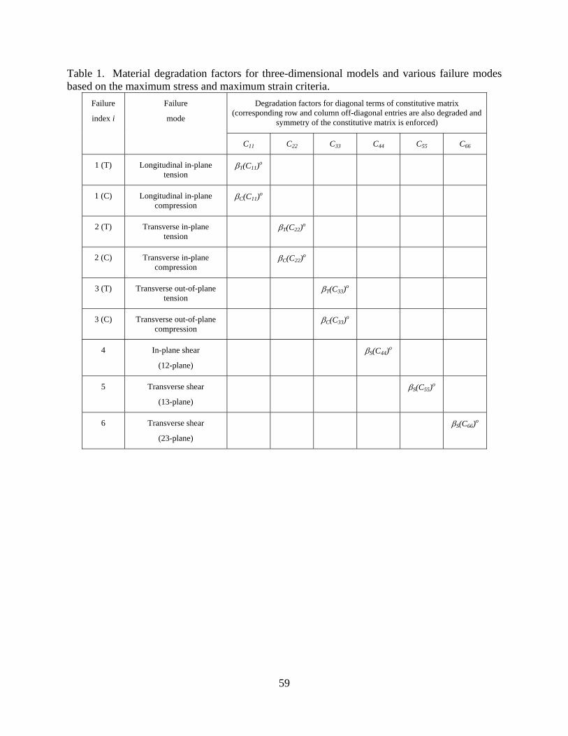
59

Table 1. Material degradation factors for three-dimensional models and various failure modes based on the maximum stress and maximum strain criteria.

Degradation factors for diagonal terms of constitutive matrix (corresponding row and column off-diagonal entries are also degraded and

symmetry of the constitutive matrix is enforced)

Failure

index i

Failure

mode

C11 C22 C33 C44 C55 C66

1 (T) Longitudinal in-plane tension

βT(C11)o

1 (C) Longitudinal in-plane compression

βC(C11)o

2 (T) Transverse in-plane tension

βT(C22)o

2 (C) Transverse in-plane compression

βC(C22)o

3 (T) Transverse out-of-plane tension

βT(C33)o

3 (C) Transverse out-of-plane compression

βC(C33)o

4 In-plane shear

(12-plane)

βS(C44)o

5 Transverse shear

(13-plane)

βS(C55)o

6 Transverse shear

(23-plane)

βS(C66)o

60

Table 2. Material degradation factors for three-dimensional models and various failure modes based on the Tsai-Wu criteria.



Failure

index i

Failure

mode

C11 C22 C33 C44 C55 C66


βT(C11)o


βC(C11)o


βT(C22)o


βC(C22)o


βT(C33)o


βC(C33)o

4 In-plane shear

(12-plane)

βS(C44)o

5 Transverse shear

(13-plane)

βS(C55)o

6 Transverse shear

(23-plane)

βS(C66)o

61

Table 3. Material degradation factors for three-dimensional models and various failure modes based on the Hashin criteria.



Failure

index i

Failure

mode

C11 C22 C33 C44 C55 C66


βT(C11)o βS(C44)o


βC(C11)o


βT(C22)o βS(C44)o


βC(C22)o βS(C44)o


βT(C33)o


βC(C33)o

4 In-plane shear

(12-plane)

βS(C44)o

5 Transverse shear

(13-plane)

βS(C55)o

6 Transverse shear

(23-plane)

βS(C66)o

62

Table 4. User-defined property data for the UMAT subroutine. PROPS array

entry, i Variable

name Description

1,2,3 Et(i) Initial elastic tension moduli: E11t, E22t, E33t 4,5,6 Ec(i) Initial elastic compression moduli: E11c, E22c, E33c 7,8,9 G0(i) Initial elastic shear moduli: G12, G13, G23

10,11,12 Anu(i) Poisson’s ratios: ν12, ν13, ν23 13,14,15 Xt(i) Ultimate tension stress allowable values in the 1-, 2-, 3-directions 16,17,18 Xc(i) Ultimate compression stress allowable values in the 1-, 2-, 3-directions 19,20,21 S(i) Ultimate shear (12-, 13-, 23-planes) stress allowable values 22,23,24 EpsT(i) Ultimate normal tension strain allowable values in the 1-, 2-, 3-directions 25,26,27 EpsC(i) Ultimate normal compression strain allowable values in the 1-, 2-, 3-

directions 28,29,30 GamS(i) Ultimate shear (12-, 13-, 23-planes) strain allowable values 31,32,33 EpsTx(i) Maximum normal tension strain allowable value in the 1-, 2-, 3-directions;

currently not used 34,35,36 EpsCx(i) Maximum normal compression strain allowable values in the 1-, 2-, 3-

directions; currently not used 37,38,39 GamSx(i) Maximum shear (12-, 13-, 23-planes) strain allowable values; currently not

used 40 GIc Critical strain energy release rate for Mode I fracture 41 FPZ Width of the fracture process zone 42 SlimT Stress limit factor for tension behavior; currently not used 43 SlimC Stress limit factor for compression behavior; currently not used 44 SlimS Stress limit factor for in-plane shear behavior; currently not used

45, 46, 47 Weibl(i) Weibull parameter of MLT model for normal stress components (i=1, 2, 3); currently not used

48, 49, 50 Weibl(j) Weibull parameter of MLT model for shear stress components (j=4, 5, 6); currently not used

51 Dgrd(1) Material degradation factor for tension failures, non-zero values result in degradation after failure initiation; active only when PDA=1 to 4

52 Dgrd(2) Material degradation factor for compression failures, non-zero values result in degradation after failure initiation; active only when PDA=1 to 4

53 Dgrd(3) Material degradation factor for shear failures, non-zero values result in degradation after failure initiation; active only when PDA=1 to 4

54 RECURS Flag for selecting the type of material degradation: 0=instantaneous, 1=recursive when PDA=1 to 4

55 PDA Progressive failure analysis option (0=linear, elastic, bimodulus response, 1=use maximum stress criteria, 2=use maximum strain criteria, 3=use Tsai-Wu polynomial, 4=use Hashin criteria)

63

Table 5. UMAT-defined solution-dependent variables. STATEV

array entry i

Solution-Dependent Variable

Name

Description of Solution-Dependent Variables

Two-dimensional shell elements, NDV=8 1 dmg(1) Degradation factor for the σ11 stress component 2 dmg(2) Degradation factor for the σ22 stress component 3 dmg(3) Degradation factor for the σ12 stress component 4 fflags(1) Failure flag for first failure mode 5 fflags(2) Failure flag for second failure mode 6 fflags(3) Failure flag for third failure mode 7 SEDtot Total strain-energy density 8 Damage Damage estimate based on energy lost (total minus

recoverable)/(fracture toughness) Three-dimensional solid elements. NDV=14

1 dmg(1) Degradation factor for the σ11 stress component 2 dmg(2) Degradation factor for the σ22 stress component 3 dmg(3) Degradation factor for the σ33 stress component 4 dmg(4) Degradation factor for the σ12 stress component 5 dmg(5) Degradation factor for the σ13 stress component 6 dmg(6) Degradation factor for the σ23 stress component 7 fflags(1) Failure flag for first failure mode 8 fflags(2) Failure flag for second failure mode 9 fflags(3) Failure flag for third failure mode 10 fflags(4) Failure flag for fourth failure mode 11 fflags(5) Failure flag for fifth failure mode 12 fflags(6) Failure flag for sixth failure mode 13 SEDtot Total strain-energy density 14 Damage Damage estimate based on energy lost (total minus

recoverable)/(fracture toughness)

Note: The degradation solution-dependent variables (SDVs) should be zero until failure initiation is detected. Once failure initiation has been detected, the degradation SDVs will be non-zero and approach a value of unity (i.e., complete degradation at that material point). The failure flag SDVs are the solution increment number when failure initiation at that material point and for that stress component is detected. Contour plots of the failure flag SDVs can be used to give an indication of the evolution of the damage progression.

64

Table 6. Summary of the peak failure loads for the cross-ply and quasi-isotropic 16-layer graphite-epoxy open-hole-tension coupons using different failure criteria, a maximum solution

increment size of 0.01, and a recursive degradation with a degradation factor β of 0.5.

Peak Failure Load, pounds

Progressive

failure Analysis

(PDA)

Cross-ply

(laminate)

Cross-ply

(smeared)

Quasi-

isotropic

(laminate)

Max. Stress (1) 9,531 10,041 7,975

Max. Strain (2) 9,620 9,996 7,941

Tsai-Wu (3) 8,655 9,466 7,869

Hashin (4) 7,129 6,056 5,985

Test Average

[120]

9,605 9,605 7,810

65

Figure 1. Typical stress-strain curve for a linear elastic-brittle bimodulus material.

Figure 2. Representative uniaxial stress-strain curve for strain-softening material –

nomenclature.

Strain

Stress

ET

EC

σTall

σCall

66

Figure 3. Geometry and boundary conditions for the demonstration problem.

Figure 4. Stress-strain curves for the two materials studied in the demonstration problems.

67

Figure 5. Stress-strain behavior for different progressive failure analysis criteria implemented within the UMAT subroutine obtained using instantaneous degradation, a degradation factor of

10-6, and a maximum solution increment size factor of 0.01.

68

(a) Axial reaction force as a function of applied strain.

(b) Material degradation factor as a function of applied strain.

Figure 6. Selected response parameters for different progressive failure analysis criteria implemented within the UMAT subroutine obtained using instantaneous degradation, a

degradation factor of 10-6, and a maximum solution increment size factor of 0.01.

69

(c) Strain energy density as a function of applied strain.

(d) Energy-based damage factor as a function of applied strain.

Figure 6. Concluded.

70

Figure 7. Stress-strain behavior for the linear elastic brittle material obtained using selected

maximum solution increment size factors, instantaneous degradation, a degradation factor of 10-

6, and the maximum stress criteria.

71

(a) Effect of different degradation factors combined with instantaneous degradation.

(b) Effect of different degradation factors combined with recursive degradation.

Figure 8. Stress-strain behavior for the linear elastic brittle material obtained using a maximum solution increment size factor of 0.01and the maximum stress criteria.

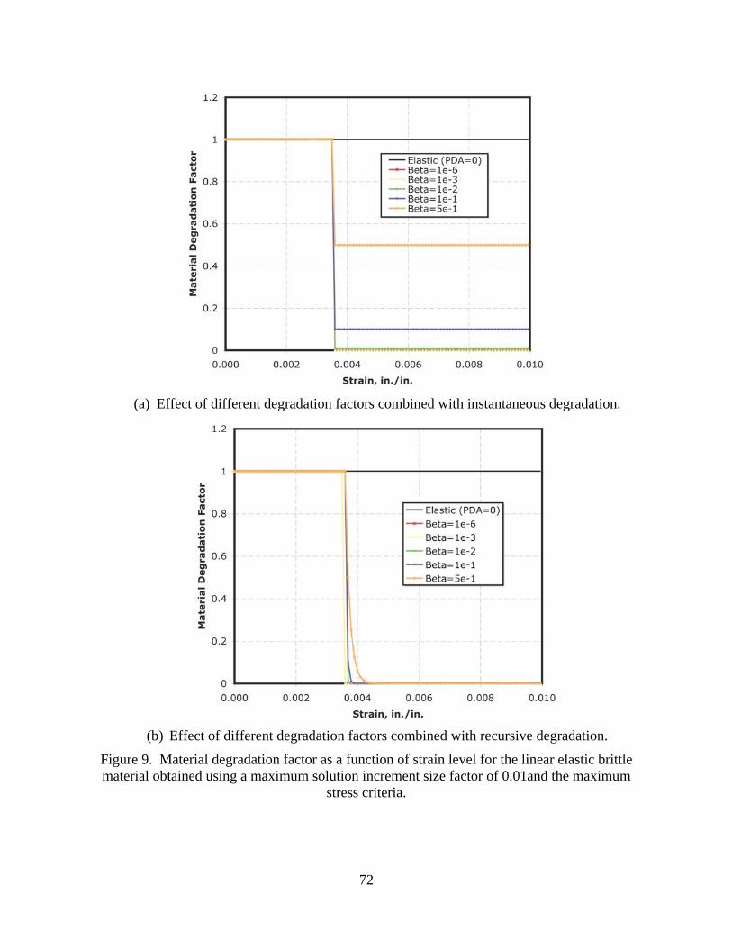
72



Figure 9. Material degradation factor as a function of strain level for the linear elastic brittle material obtained using a maximum solution increment size factor of 0.01and the maximum

stress criteria.

73



Figure 10. Strain energy density predictions for the linear elastic brittle material obtained using a maximum solution increment size factor of 0.01and the maximum stress criteria.

74

Figure 11. Stress-strain behavior predicted using the maximum stress and maximum strain

criteria with instantaneous degradation, a degradation factor of 10-6, and a maximum solution increment size factor of 0.01 and applied to the nonlinear elastic brittle material.

Figure 12. Stress-strain behavior predicted using the maximum strain criteria with recursive

degradation, a degradation factor of 10-6, and a maximum solution increment size factor of 0.01 and applied to the nonlinear elastic brittle material.

75

(a) Complete model. (b) Close-up view of region near the hole.

Figure 13. Finite element model of the open-hole-tension coupon.

76

(a) Predictions obtained using a 0.02 value for the maximum solution increment size.

(b) Predictions obtained using a 0.01 value for the maximum solution increment size.

Figure 14. Comparison of different progressive failure analysis models for the 16-ply cross-ply open-hole-tension coupon using recursive degradation with a degradation factor β of 0.5.

77

(a) Results using maximum strain criteria (PDA=2).

(b) Results using Hashin criteria (PDA=4).

Figure 15. Influence of maximum solution increment size on the progressive failure predictions for the 16-ply cross-ply open-hole-tension coupon using recursive degradation with a

degradation factor β of 0.5.

78

(a) Results using maximum strain criteria (PDA=2).

(b) Results using Hashin criteria (PDA=4).

Figure 16. Influence of degradation factor β on the progressive failure predictions for the 16-ply

cross-ply open-hole-tension coupon using recursive degradation and a maximum solution increment size of 0.02.

79

Figure 17. Influence of maximum solution increment size on the progressive failure predictions for the 16-ply cross-ply open-hole-tension coupon using the maximum strain criteria (PDA=2)

and instantaneous degradation with a degradation factor β of 10-6.

Figure 18. Comparison of different progressive failure analysis models for the 16-ply quasi-

isotropic open-hole-tension coupon using recursive degradation with a degradation factor β of 0.5 and a maximum solution increment size of 0.01.

80

Figure C1. Representative uniaxial stress-strain curve for MLT material model – nomenclature.

81

(a) Predicted stress-strain response.

(b) State variable ω as a function of strain.

Figure C2. Predicted uniaxial response for different values of SLIM when initial and secant moduli are equal (E0=2 Msi, XT=5,000 psi, and εult=0.0025 in./in., EROD=0.008).

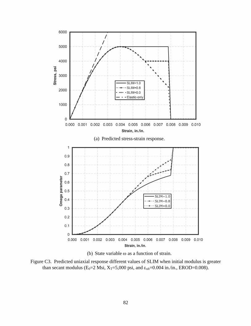
82



Figure C3. Predicted uniaxial response different values of SLIM when initial modulus is greater than secant modulus (E0=2 Msi, XT=5,000 psi, and εult=0.004 in./in., EROD=0.008).

83



Figure C4. Predicted uniaxial response for different values of the initial modulus E0 (XT=5,000 psi, and εult=0.004 in./in., SLIM=0.0, EROD=0.008).

84

Figure C5. Effect of the ratio of initial modulus to secant modulus β on the internal state

variable ω as a function of strain (XT=5,000 psi, and εult=0.004 in./in., SLIM=0.0, EROD=0.008).

REPORT DOCUMENTATION PAGE Form ApprovedOMB No. 0704-0188

2. REPORT TYPE Contractor Report

4. TITLE AND SUBTITLE

User-Defined Material Model for Progressive Failure Analysis5a. CONTRACT NUMBER

6. AUTHOR(S)

Knight, Norman F., Jr.

7. PERFORMING ORGANIZATION NAME(S) AND ADDRESS(ES)

NASA Langley Research Center General DynamicsHampton, VA 23681-2199 Advanced Information Systems 14700 Lee Road Chantilly, VA 20151 9. SPONSORING/MONITORING AGENCY NAME(S) AND ADDRESS(ES)

National Aeronautics and Space AdministrationWashington, DC 20546-0001

8. PERFORMING ORGANIZATION REPORT NUMBER

10. SPONSOR/MONITOR'S ACRONYM(S)

NASA

13. SUPPLEMENTARY NOTESPrepared for Langley Research Center under GSA Task Order GS-00F-0067M, NASA Order No. NNL06AA48T.Langley Technical Monitor: James R. ReederAn electronic version can be found at http://ntrs.nasa.gov

12. DISTRIBUTION/AVAILABILITY STATEMENTUnclassified - UnlimitedSubject Category 39Availability: NASA CASI (301) 621-0390

19a. NAME OF RESPONSIBLE PERSON

STI Help Desk (email: [email protected])

14. ABSTRACT

An overview of different types of composite material system architectures and a brief review of progressive failure materialmodeling methods used for structural analysis including failure initiation and material degradation are presented. Differentfailure initiation criteria and material degradation models are described that define progressive failure formulations. Theseprogressive failure formulations are implemented in a user-defined material model (or UMAT) for use with theABAQUS/Standard nonlinear finite element analysis tool. Implementation details and use of the UMAT subroutine aredescribed in the present paper. Parametric studies for composite structures are discussed to illustrate the features of theprogressive failure modeling methods that have been implemented.

15. SUBJECT TERMSProgressive failure analysis; Nonlinear analysis; Composite structures

18. NUMBER OF PAGES

9319b. TELEPHONE NUMBER (Include area code)

(301) 621-0390

a. REPORT

U

c. THIS PAGE

U

b. ABSTRACT

U

17. LIMITATION OF ABSTRACT

UU

Prescribed by ANSI Std. Z39.18Standard Form 298 (Rev. 8-98)

3. DATES COVERED (From - To)

5b. GRANT NUMBER

5c. PROGRAM ELEMENT NUMBER

5d. PROJECT NUMBER

NNL06AA48T5e. TASK NUMBER

Task 105f. WORK UNIT NUMBER

732759.07.09

11. SPONSOR/MONITOR'S REPORT NUMBER(S)

NASA/CR-2006-214526

16. SECURITY CLASSIFICATION OF:

The public reporting burden for this collection of information is estimated to average 1 hour per response, including the time for reviewing instructions, searching existing data sources, gathering and maintaining the data needed, and completing and reviewing the collection of information. Send comments regarding this burden estimate or any other aspect of this collection of information, including suggestions for reducing this burden, to Department of Defense, Washington Headquarters Services, Directorate for Information Operations and Reports (0704-0188), 1215 Jefferson Davis Highway, Suite 1204, Arlington, VA 22202-4302. Respondents should be aware that notwithstanding any other provision of law, no person shall be subject to any penalty for failing to comply with a collection of information if it does not display a currently valid OMB control number.PLEASE DO NOT RETURN YOUR FORM TO THE ABOVE ADDRESS.

1. REPORT DATE (DD-MM-YYYY)

12 - 200601-

user-defined material model for progressive failure … user-defined material model for progressive...

Documents