factors influencing progressive failure analysis predictions for laminated composite ... · ·...

American Institute of Aeronautics and Astronautics

092407

1

Factors Influencing Progressive Failure Analysis Predictions for Laminated Composite Structure

Norman F. Knight, Jr.1 General Dynamics – Advanced Information Systems, Chantilly, VA 20151

Progressive failure material modeling methods used for structural analysis including failure initiation and material degradation are presented. Different failure initiation criteria and material degradation models are described that define progressive failure formulations. These progressive failure formulations are implemented in a user-defined material model for use with a nonlinear finite element analysis tool. The failure initiation criteria include the maximum stress criteria, maximum strain criteria, the Tsai-Wu failure polynomial, and the Hashin criteria. The material degradation model is based on the ply-discounting approach where the local material constitutive coefficients are degraded. Applications and extensions of the progressive failure analysis material model address two-dimensional plate and shell finite elements and three-dimensional solid finite elements. Implementation details are described in the present paper. Parametric studies for laminated composite structures are discussed to illustrate the features of the progressive failure modeling methods that have been implemented and to demonstrate their influence on progressive failure analysis predictions.

I. Introduction Advanced composite structures are a challenge to analyze. This challenge is driven by the evolution of new

material systems and novel fabrication processes. Analytical procedures available in commercial nonlinear finite element analysis tools for modeling these new material forms are often lagging behind the material science developments. That is to say, analytical models implemented in the analysis tools must frequently be “engineered” for new material systems through the careful extension, within the known limits of applicability, of existing material models available in the analysis tools. When the materials technology matures sufficiently, verified analytical models can be developed, validated, and become available in the commercially available tools. In the interim, some commercial finite element analysis tool developers have responded to user needs by providing a capability to embed user-defined, special-purpose finite elements and material models.

This need for a capability to explore user-defined material models exists – particularly for composite structures. Composite material systems have unique characteristics and capabilities not seen in metals. These characteristics include being brittle rather than ductile, being directional in stiffness and strength, and being applicable to different fabrication architectures. These characteristics enable advanced design concepts including structural tailoring, multifunctional features, and performance enhancements.

Another consideration for the material model developer is the intended application and target finite element analysis tool. Applications involving an explicit transient dynamic nonlinear tool impose different requirements on the material model developer than applications involving implicit (or quasi-static) nonlinear tools. In explicit formulations, only the current stress state is needed to evaluate the current internal force vector in order to march the transient solution forward in time. In implicit (or quasi-static) formulations, the current stress state and a consistent local tangent material stiffness matrix are needed to form the internal force vector for the residual (imbalance) force vector computation and to form the tangent stiffness matrix for the Newton-Raphson iteration procedure.

The objective of the present paper is to describe a progressive failure analysis methodology [1] that is applicable to laminated composite structures and focuses on implicit, quasi-static applications. This material model accounts for a linear elastic-brittle bimodulus material behavior. Several options for detecting failure initiation and subsequent damage progression are provided in this user-defined material model. The material model can be

1 Chief Engineer, Structural Mechanics. Associate Fellow AIAA, Fellow ASME.

https://ntrs.nasa.gov/search.jsp?R=20080015744 2018-06-27T00:58:18+00:00Z


092407

2

applied even when only laminate-level or “apparent” material data rather than lamina-level data are available. Factors influencing the progressive failure analysis prediction are identified and discussed. Implementation of the material model for progressive failure analysis is demonstrated using the user-defined material modeling (or UMAT) feature provided in the ABAQUS/Standard2 nonlinear finite element analysis tool [2].

The present paper is organized in the following way. First, a brief overview of composite materials is presented to define terminology. Second, the basic equations for constitutive modeling in two- and three-dimensions are described. Next, the failure initiation and material degradation models proposed for use with laminated composites are defined. Then, the nonlinear solution process and implementation details of the material model for traditional progressive failure analyses are described. Numerical results and discussion are presented for a 16-ply open-hole-tension coupon using two different stacking sequences. Concluding remarks are given in the final section of the paper.

II. Composite Materials Composite materials can be defined as materials comprised of more than one material, such as a bimetallic strip

or as concrete (e.g., see Refs. [3-8]). However, composite materials are more commonly defined as materials formed using fiber-reinforced materials combined with some matrix material (e.g., graphite fibers embedded in an epoxy resin system). Typical fiber materials include graphite and glass, and typical matrix materials include polymer, metallic, ceramic, and phenolic materials. Composite material systems are available as unidirectional or textile laminas that are used to design laminated composite structures. Background material and issues are briefly described in the next subsections.

A. Unidirectional Laminated Composites

Unidirectional laminated composite structures are formed by stacking (or laying up) unidirectional lamina with each layer having different properties and/or different orientations in order to form a composite laminate of a given total thickness. The elastic analysis of such composite structures is well developed [3-8]. Typically, composite structures are thin structures that are modeled using two-dimensional plate or shell elements formulated in terms of stress resultants and based on an assumed set of kinematical relations. Hence, pre-integration through the shell thickness is performed and the constitutive relations are in terms of resultant quantities rather than point stresses and strains. Integrating the constitutive relations through the thickness generates the so-called “ABD” stiffness coefficients where the “A” terms denote membrane, the “B” terms denote membrane-bending coupling, and the “D” terms denote bending stiffness coefficient matrices, respectively. However, in some cases, composite structures are relatively thick and require three-dimensional modeling and analysis.

Material characterization of laminated composite structures has been demonstrated to be quite good, and failure prediction models for damage modes associated with fiber failure in polymeric composites have also been successful. Ochoa and Reddy [5] present an excellent discussion of progressive failure analyses. In laminated composite structures, fiber-dominated failure modes (e.g., axial tension) are better-understood and analyzed than matrix-dominated failure modes (e.g., axial compression, transverse tension). Methods to predict failure initiation (e.g., see Refs. [9-11]) and to perform material degradation remain active areas of research. Material degradation can be performed using a ply-discounting approach or an internal state variable approach based on continuum damage mechanics. Most composite failure analysis methods embedded within a finite element analysis tool perform a point-stress analysis, evaluate failure criteria, possibly degrade material properties, and then continue to the next solution increment (e.g., see Refs. [12-31]). Application of progressive failure analysis methods to postbuckled composite structures continues to challenge analysts due to the complexity and interaction of failure modes with the nonlinear structural response (e.g., see Refs. [15-20, 23, 28, 29]).

Damage associated with matrix cracking, the onset of delaminations, and crack growth is very difficult to predict for laminated composite structures. Failure analysis procedures based on the use of overlaid two-dimensional meshes of shell finite elements [23], the use of computed transverse stress fields from the equilibrium equations [15], and the use of decohesion or interface elements [29, 32-36] have met with limited success. Analytical methods for predicting matrix cracking, delamination, and crack growth are still immature while current research associated with decohesive models appears promising, these failure prediction models require additional material properties obtained from further testing and material characterization.

2 ABAQUS/Standard is a trademark of ABAQUS, Inc.


092407

3

B. Woven-Fabric Laminated Composites

Woven-fabric laminated composite structures (e.g., see Refs. [37-44]) can be formed by laying up woven-fabric layers or by weaving through the total thickness. Fabric layers usually have interwoven groups of fibers in multiple orientations. Plain- and satin-weave fabrics have warp and weft (0-degree and 90-degree, respectively) yarns only. Woven-fabric laminated composites are different from unidirectional-based laminated composites, and different analysis methods are needed. Often, however, plain- and satin-weave fabrics of a given thickness are modeled as an equivalent set of two unidirectional layers (i.e., [0/90]) where each unidirectional layer has half the fabric layer thickness. Alternatively, a single fabric layer is modeled as an “equivalent” single layer of the same thickness and having equal in-plane longitudinal and transverse moduli (E11=E22). This equivalence is a modeling simplification and does not accurately represent the micromechanics of the woven-fabric composite. When only “apparent” material data are available (i.e., only laminate-level material data), failure initiation criteria should be defined in a manner consistent with the available data [44]. As such, the through-the-thickness material definition is smeared over the laminate, and lamina properties are essentially those of identical orthotropic layers with E1 and E2 being equal to the corresponding effective engineering values (Ex and Ey) obtained from a laminate analysis. An average lamina thickness is defined as the local laminate thickness divided by the number of apparent ply layers.

III. Constitutive Models The constitutive models in a quasi-static stress analysis relate the state of strain to the state of stress. These

relations may be different depending on the kinematic assumptions of the formulation (e.g., different through-the-thickness assumptions for the displacement fields). However, in performing point strain analyses, the state of stress at a point is desired and is readily computed once the point strains are determined through the use of the kinematics relations. Dimensional reduction may result in one or more of the stress components being assumed to be zero. For two-dimensional models, C0 plate and shell kinematics models have five non-zero components and typically account at least for constant non-zero transverse shear stresses through the thickness, while C1 plate and shell kinematics models have only three stress components and neglect transverse stresses. For three-dimensional models, six stress and six strain components are evaluated. The subsequent sections describe the constitutive relations for these kinematics models. Additional details on laminated composite structures are provided in Refs. [3-8]. The engineering material constants appearing in subsequent equations are the linear elastic mechanical property values ) and ,, , , , ,, , (e.g., 231312231312332211 νννGGGEEE .

A. Two-Dimensional Material Model

In two dimensions, the strain-stress relations for a typical linear elastic orthotropic material used with two-dimensional plate and shell elements based on C0 continuity requirements and implemented within ABAQUS are written as:

ε{ }=

ε11

ε22

γ12

γ13

γ 23

⎧

⎨

⎪ ⎪ ⎪

⎩

⎪ ⎪ ⎪

⎫

⎬

⎪ ⎪ ⎪

⎭

⎪ ⎪ ⎪

=

S110 S12

0 0 0 0S21

0 S220 0 0 0

0 0 S440 0 0

0 0 0 S550 0

0 0 0 0 S660

⎡

⎣

⎢ ⎢ ⎢ ⎢ ⎢ ⎢

⎤

⎦

⎥ ⎥ ⎥ ⎥ ⎥ ⎥

σ11

σ 22

σ12

σ13

σ 23

⎧

⎨

⎪ ⎪ ⎪

⎩

⎪ ⎪ ⎪

⎫

⎬

⎪ ⎪ ⎪

⎭

⎪ ⎪ ⎪

= S0[ ] σ{ } (1)

For C1 shell elements, the terms associated with the transverse or interlaminar shear effects (i.e., terms associated with γ13 and γ23) are neglected. It is clear from Eq. 1 that the normal components are coupled to one another, while the shear components are completely uncoupled. The compliance coefficients Sij

0 in this matrix are defined in terms of the elastic engineering material constants (see Ref. [2], Vol. II, p. 10.2.1-3). Namely, the non-zero terms are:


092407

4

S110 =

1E11

; S220 =

1E22

;

S120 = S21

0 = −ν 21

E22

= −ν12

E11

;

S440 =

1G12

; S550 =

1G13

; S660 =

1G23

(2)

Hence, the stress-strain relations can be obtained directly from the compliance relations given in Eq. 1 as:

σ{ }=

σ11

σ 22

σ12

σ13

σ 23

⎧

⎨

⎪ ⎪ ⎪

⎩

⎪ ⎪ ⎪

⎫

⎬

⎪ ⎪ ⎪

⎭

⎪ ⎪ ⎪

=

C110 C12

0 0 0 0C21

0 C220 0 0 0

0 0 C440 0 0

0 0 0 C550 0

0 0 0 0 C660

⎡

⎣

⎢ ⎢ ⎢ ⎢ ⎢ ⎢

⎤

⎦

⎥ ⎥ ⎥ ⎥ ⎥ ⎥

ε11

ε22

γ12

γ13

γ 23

⎧

⎨

⎪ ⎪ ⎪

⎩

⎪ ⎪ ⎪

⎫

⎬

⎪ ⎪ ⎪

⎭

⎪ ⎪ ⎪

= S0[ ]−1ε{ }= C 0[ ]ε{ } (3)

Note that the order of the stress and strain terms is defined by the convention used by ABAQUS. The stiffness coefficients Cij

0 in this matrix are defined in terms of the elastic material constants (see Ref. [2], Vol. II, p. 10.2.1-3). Namely,

C110 = E11

Δ; C22

0 = E22

Δ;

C12

0 = C210 =

ν12E22

Δ=

ν 21E11

Δ;

C440 = G12; C55

0 = G13; C660 = G23

Δ =1−ν12ν 21

(4)

and based on the reciprocity relation for plane elasticity given by:

E11ν 21 = ν12E22 (5)

In this approach, the material is modeled implicitly through the thickness by using the kinematics assumptions of the two-dimensional shell elements (i.e., in-plane strains vary linearly through the shell thickness and the transverse normal strain is zero). Typically, the in-plane shear stress-shear strain relationship is assumed to be linear; however, nonlinear in-plane normal stress behavior as well as Hahn-type in-plane shear nonlinearity [45, 46] can be incorporated as part of a material model. In addition, shear correction factors for orthotropic laminates can be computed using the approach presented by Whitney [47].

Similarly, the stress-strain relations for a typical linear elastic orthotropic material used with two-dimensional plate and shell elements based on the C1 continuity requirements are written as:

{σ} =σ11

σ 22

σ12

⎧

⎨ ⎪

⎩ ⎪

⎫

⎬ ⎪

⎭ ⎪ =

C110 C12

0 0C21

0 C220 0

0 0 C440

⎡

⎣

⎢ ⎢ ⎢

⎤

⎦

⎥ ⎥ ⎥

ε11

ε22

γ12

⎧

⎨ ⎪

⎩ ⎪

⎫

⎬ ⎪

⎭ ⎪ = [C0]{ε} (6)

where the Cij0 coefficients are defined in Eq. 4.

At each planar Gaussian integration point within each plate or shell element surface plane (e.g., 2×2 Gaussian integration points for a fully integrated two-dimensional plate or shell element), material points through the entire thickness (referred to as section points in ABAQUS) are evaluated to determine the through-the-thickness state of strain and to estimate the trial stresses (i.e., point stresses and strains).


092407

5

Implicit in the previous discussion is the assumption that the elastic response is the same in tension and compression; however, some composite systems exhibit a bimodulus behavior. A bimodulus elastic orthotropic material exhibits a different stress-strain response in tension and compression. Basic constitutive relations for a bimodulus material are presented by Ambartsumyan [48], Tabaddor [49], Jones [50], Bert [51], Reddy and Chao [52], and Vijayakumar and Rao [53]. However, such a material model for a modern composite material is not readily available in most commercial general-purpose finite element tools. In some cases, various options can be combined or semi-automated procedures developed to address bimodulus composite material systems. In a linear stress analysis, for example, a material iterative process to assign material properties can be used that defines the appropriate material properties based on the local principal strains. Such a material iterative process is typically performed manually or it may be a semi-automated process, and the process needs to be repeated for each different loading case since the local strain state changes. For a nonlinear analysis that accounts for material degradation and damage, a semi-automatic material iteration approach is not viable. In such cases, user-defined material models can be developed for certain commercial finite element tools (e.g., ABAQUS/Standard). Alternatively, “engineering” models (e.g., use only the tensile modulus, use an average modulus, or some other engineering approximation for the material response) can be developed that approximate the mechanical behavior provided these approximations are defined and limitations are understood by the end-users (or stakeholders) of the analysis results. The next section describes failure initiation (or failure detection) criteria commonly used with laminated composite structures

IV. Failure Initiation Criteria Having described the basic constitutive models for two-dimensional formulations for the recovery of stresses at a

material point in a composite structure, the failure initiation criteria implemented in this UMAT subroutine for ABAQUS/Standard are now described. Four common failure initiation criteria have been implemented; namely, the maximum stress criteria, the maximum strain criteria, the Tsai-Wu failure polynomial [9, 17, 18, 27], and the Hashin criteria [11]. Both two- and three-dimensional implementations of these criteria are required depending on whether the finite element model of the structural component involves two-dimensional shell elements or three-dimensional solid elements, and both implementations are included within this single UMAT subroutine. Even though transverse shear behavior is not treated explicitly within an ABAQUS/Standard UMAT subroutine, their failure criteria are defined herein for completeness.

The stresses in the material coordinate system are computed within the current UMAT subroutine using the given strains and the material stiffness coefficients at each material point. Having these stresses, the stress-based failure criteria are evaluated, and material degradation is imposed as warranted. In the following subsection, the Hashin failure criteria implemented within the current UMAT subroutine is described. The other criteria implemented in this UMAT subroutine are described in Ref. [1]. Later, in a separate section of the present paper, the material degradation approach is described.

A. Hashin Failure Criteria

The Hashin failure criteria [11] are also interacting failure criteria as the failure criteria use more than a single stress component to evaluate different failure modes. The Hashin criteria were originally developed as failure criteria for unidirectional polymeric composites, and hence, application to other laminate types or non-polymeric composites represents a significant approximation. Usually, the Hashin criteria are implemented within a two-dimensional classical lamination approach for the point-stress calculations with ply discounting as the material degradation model. Failure indices for the Hashin criteria are related to fiber and matrix failures and involve four failure modes. Additional failure indices result from extending the Hashin criteria to three-dimensional problems wherein the extensions are simply the maximum stress criteria for the transverse normal stress component. The failure modes included with the Hashin criteria [11] when extended to three dimensions are:

• Tensile fiber failure – for 011 ≥σ

e1t( )2

=σ11

XT

⎛

⎝ ⎜

⎞

⎠ ⎟

2

+σ12

2 + σ132

S122 =

>1 failure≤1 no failure

⎧ ⎨ ⎩

(7)


092407

6

• Compressive fiber failure – for 011 <σ

e1c( )2

=σ11

XC

⎛

⎝ ⎜

⎞

⎠ ⎟

2

=>1 failure≤1 no failure

⎧ ⎨ ⎩

(8)

• Tensile matrix failure – for σ 22 + σ 33 > 0

e2t( )2

=σ 22 + σ 33( )2

YT2 +

σ 232 −σ 22σ 33( )

S232 +

σ122 + σ13

2

S122 =


⎧ ⎨ ⎩

(9)

• Compressive matrix failure – for σ 22 + σ 33 < 0

e2c( )2

=YC

2S23

⎛

⎝ ⎜

⎞

⎠ ⎟

2

−1⎡

⎣ ⎢ ⎢

⎤

⎦ ⎥ ⎥ σ 22 +σ 33

YC

⎛

⎝ ⎜

⎞

⎠ ⎟ +

σ 22 +σ 33( )2

4S232

+σ 23

2 −σ 22σ 33( )S23

2 +σ12

2 +σ132

S122 =


⎧ ⎨ ⎪

⎩ ⎪

(10)

• Interlaminar normal tensile failure – for σ 33 > 0

e3t( )2

=σ 33

ZT

⎛

⎝ ⎜

⎞

⎠ ⎟

2


⎧ ⎨ ⎪

⎩ ⎪ (11)

• Interlaminar normal compression failure – for σ 33 < 0

e3c( )2

=σ 33

ZC

⎛

⎝ ⎜

⎞

⎠ ⎟

2


⎧ ⎨ ⎪

⎩ ⎪ (12)

In these failure criteria, lamina strength allowable values for tension and compression in the lamina principle material directions (fiber or 1-direction and matrix or 2-direction) as well as the in-plane shear strength allowable value are denoted by XT, XC, YT, YC, and S12, respectively, ZT and ZC are the transverse normal strength allowable values in tension and compression, respectively, and S13 and S23 are the transverse shear strength allowable values. In Eqs. 7-12, the in-plane normal and shear stress components are denoted by σij (i, j=1, 2). The failure indices for the transverse normal stress component σ33 are based on the maximum stress criteria for tension and compression, as indicated by Eqs. 11 and 12. Finally, failure indices for tension and compression are then compared to unity to determine whether failure initiation is predicted. If any failure index ei

t,c exceeds unity, then failure initiation has occurred for that stress component at that material point and material degradation will be performed. That is, each failure mode may fail independently at different load levels, and the Hashin failure flags fi

H are set accordingly:

f iH =

0 for eit,c ≤ 1

±1 for eit,c > 1

⎧ ⎨ ⎩

for i = 1, 3 (13)

Once a failure flag is nonzero, material degradation is performed as described in the next section. Also, once a failure flag becomes nonzero, it remains nonzero (i.e., no self healing of the material is permitted).

V. Damage Progression Models Previous sections described the constitutive models and the failure initiation criteria implemented in the current

UMAT subroutine. This section presents the damage progression strategies that provide material degradation and also the heuristics associated with the material degradation models for these failure initiation criteria. Various material degradation models have been proposed and demonstrated for laminated composite structures (e.g., see Refs. [12-36]). These models may be generally categorized into two main groups: heuristic models based on a ply-discounting material degradation approach and models based on a continuum-damage-mechanics (CDM) approach


092407

7

using internal state variables. Representative models for the ply-discounting material degradation approach are implemented within the current UMAT subroutine [1]; however, both approaches are described subsequently in the present paper.

A. Ply-Discounting Approach

Traditionally, ply-discounting material degradation models are based on the degradation (or discounting) of the elastic material stiffness coefficients by a value βI that, in essence, generates a diminishing stiffness value (i.e., approaches zero as the number of solution increments from failure initiation increases) for the ith stress component. In this strategy, the ith diagonal entry of the elastic constitutive matrix Cii

0 is set equal to βI multiplied by Cii0 , and

the other row and column entries of the elastic constitutive matrix [C0] are also degraded in a similar manner. Another ply-discounting strategy involves degrading the elastic mechanical properties of the material directly (i.e., assumption of vanishing elastic moduli after failure initiation is detected) and then re-computing the local material stiffness coefficients using the degraded mechanical properties. In this strategy, special care needs to be given to maintain symmetry in the degraded constitutive matrix.

The application of material degradation implemented in this UMAT subroutine is related to the rate of material degradation once failure initiation is detected. Instantaneous or single-step degradation degrades the material stiffness coefficients only once by the degradation factor. Typical values for the degradation factor can range from a very small value (e.g., 10-6) to a large value (e.g., 0.8) for this type of material degradation. Recursive degradation successively degrades the material stiffness coefficients in a gradual manner. When the degradation factor is not small (e.g., say 0.5), then some of the numerical convergence issues associated with an instantaneous local change in material stiffness are avoided. Specifying recursive degradation with a near-zero degradation factor is nearly equivalent to specifying instantaneous degradation with the same near-zero factor.

Methods based on recursive material degradation have been implemented to minimize the computational impact of localized changes in material stiffness terms, and the recursive degradation option is included in the current UMAT subroutine implementation. Artificial viscous damping has also been used to improve the convergence behavior of the nonlinear solution procedure in quasi-static analyses [14, 28]. Examples of the ply-discounting approach and related computational details are presented in Refs. [15-20, 28]. The ply-discounting approach based on degrading the constitutive matrix coefficients including options for either recursive or single-step (instantaneous) material degradation (controlled by the parameter RECURS) has been implemented in the current UMAT subroutine and is available as a user-specified option.

For the ply-discounting models, the analyst selects the failure initiation criterion (PDA), the material degradation factor (β), and the type of degradation (instantaneous or recursive). The failure initiation criteria implemented in this UMAT subroutine are the maximum stress criteria (PDA=1), maximum strain criteria (PDA=2), Tsai-Wu failure polynomial (PDA=3), and the Hashin criteria (PDA=4). The form of the material degradation is selected by the parameter RECURS. When RECURS equals zero, instantaneous degradation is imposed. When RECURS equals unity, recursive degradation is imposed. Material degradation is also dependent on the failure mode (tension, compression, or shear) and independent degradation factors can be specified in this UMAT subroutine (i.e., Dgrd(1) for tension, Dgrd(2) for compression, and Dgrd(3) for shear). The material degradation factor implemented in this UMAT subroutine multiplies the material stiffness coefficients directly rather than multiplying the engineering material properties themselves. By multiplying the stiffness coefficients directly, the issue of maintaining the reciprocity relations for degraded engineering material properties is avoided.

The combined use of recursive degradation (RECURS=1) and a fractional degradation factor (e.g., β=0.5) can provide a gradual degradation of material stiffness over several solution increments in an attempt to mitigate numerical convergence difficulties attributed to near singularities in the stiffness matrix caused by localized material failures. In the present paper, the degradation factor β will be shown to have a significant effect on the failure prediction. The numerical studies reported here use a degradation factor of 0.5 as a default value for β. This value gives successive reductions in the stiffness coefficients by a factor of two on each solution increment after initial failure has been detected. While somewhat arbitrary, this value has been shown to give good convergence behavior for the overall nonlinear solution algorithm applied to progressive failure simulations.

For each failure initiation criteria, six failure indices ei are evaluated for the three-dimensional analysis models. Failure initiation is defined when one or more of these failure indices reach or exceed unity. For the various criteria, the material degradation rules follow the heuristics available in the literature. Typically, when a failure is detected


092407

8

in a particular mode, say when the first failure flag is nonzero, then the local material stiffness associated with the fiber direction is degraded.

This approach to material degradation may lead to very conservative predictions for interacting failure initiation criteria. For example, the tensile fiber failure mode given by Eq. 7 for the Hashin [11] criteria in the present UMAT subroutine implementation will result in a degradation of the fiber related stiffness coefficients as well as the in-plane shear coefficients. However, if the first term in Eq. 7 is close to unity but does not cause failure initiation (maximum stress comparison) but the entire term does exceed unity, then the failure mode could be interpreted as a fiber-matrix shearing failure mode wherein only the in-plane shear stiffness coefficients are degraded. While Hashin [11] developed failure initiation criteria, no material degradation rules were presented.

In this UMAT subroutine, the ply-discounting material degradation models are based on discounting (or degrading) the terms of the elastic stiffness constitutive matrix (i.e., Cij

Degraded = βICij0). Degradation factors βI are

defined for three failure types: tension-failure degradation factor βT, compression-failure degradation factor βC, and shear-failure degradation factor βS. Off-diagonal terms in the constitutive coefficient matrix along the same row and column are also degraded in the same manner. Material degradation can be performed either only once when failure initiation is detected (single-step approach), or it can be done recursively on each solution increment after failure initiation is detected (recursive approach). Recursive material degradation typically provides a more “gentle” process of degrading material stiffness data and potentially can improve convergence characteristics of the solution procedure compared to an “abrupt” single-step degradation approach using near zero values for the degradation factors. In addition, once a failure mode is detected, that failure mode is not checked at that material point again; however, recursive degradation of the material stiffness coefficients will continue to be applied. Material degradation continues until the degradation factor reaches a specified minimum value, and then it is held constant at that minimum value (currently set to a value of 10-30). At subsequent solution increments, other failure modes within a given failure criteria are evaluated at that material point and potentially could lead to a subsequent failure in a different mode.

B. Internal State Variable Approach

Continuum-damage-mechanics (or CDM) models generally describe the internal damage in the material by defining one or more internal state variables. Regardless of the damage state, these CDM models still represent the material as continuum having smooth, continuous field equations. Krajcinovic [54] described CDM “as a branch of continuum solid mechanics characterized by the introduction of a special (internal) field variable representing, in an appropriate (statistical) sense, the distribution of microcracks locally.” Early continuum damage mechanics work for metal structures is discussed by Lemaitre [55]. Talreja [56] was one of the earliest to propose such a model for laminated composites along with Chang and Chang [14]. Ladevèze and LeDantec [57], Shahid and Chang [58], and Barbero and Lonetti [24] have additional CDM models. CDM models express the constitutive relations in a manner similar to the elastic constitutive relations given previously, except that the coefficients (i.e., either compliance coefficients, stiffness coefficients, or the mechanical properties themselves) are functions of one or more internal state variables. CDM models also generally require additional material data as part of the material property definition. For example, one may require a material strength allowable value to be defined as a function of internal state variables, which may themselves be dependent on laminate stacking sequence. As such, their use requires even more care than material degradation models based on heuristic rules as used in ply-discounting material degradation models. Krajcinovic [59] provides additional details on CDM methods for damage modeling.

One approach is to incorporate the statistical nature of the material into the constitutive relations. Matzenmiller et al. [60] proposed such a model (called the MLT model) based on the use of a Weibull function [61] to describe the statistical nature of internal defects and the ultimate strength of a fiber bundle within a composite lamina. In the MLT model, the Weibull factor m is a primary control parameter that affects the strain-energy density at a given material point. By adjusting the value m, the degree of strain softening in the post-ultimate region is controlled. Nonlinearity in the pre-ultimate region is controlled by the independent specification of the ultimate stress value, the ultimate strain value, and a parameter similar to a material modulus.

Creasy [62] developed a different model based on the Weibull function, and Moas and Griffin [20] also used Weibull functions in their material degradation model. Hahn and Tsai [63] considered the post-ultimate behavior of symmetric cross-ply laminates. Their results indicate that a gradual degradation of the cross-ply stiffness terms explains the bilinear stress-strain behavior that occurred prior to total failure. Furthermore, they suggested that any failed lamina continues to carry its failure load in the post-ultimate range until the laminate fails (see Refs. [63, 64]).


092407

9

Hence, Schweizerhof et al. [65] incorporated a stress limit factor that sets the minimum stress value in the post-ultimate regime of the stress-strain curve. The MLT model as extended by Schweizerhof et al. [65] is available in LS-DYNA3 [66] as MAT58.

VI. Nonlinear Solution Process The very nature of a progressive failure analysis implies a nonlinear solution process is required. The

framework for the present study is ABAQUS/Standard – an implicit nonlinear finite element analysis tool [2] that provides a user-defined material modeling interface using a UMAT subroutine. Having a user-defined material feature is becoming an increasingly important capability for commercial finite element software systems. Developers of commercial finite element analysis tools frequently provide entry points for material data through special features and well-documented definition of the subroutine calling arguments. The user is given various computational results from the element routines and solution procedure that are passed to the UMAT subroutine through the calling arguments. These values may be used to determine new trial values for the stresses and constitutive coefficients based on the current deformation state.

In an ABAQUS/Standard analysis, the analyst defines various analysis “steps” to perform. Within each “step”, a number of solution increments may be performed depending on the type of analysis for that solution step. ABAQUS uses the concept of an accumulated “pseudo-time” to cover all types of solution steps within a complete implicit nonlinear analysis and a separate “pseudo-time” variable for each individual solution step. In a quasi-static analysis, “pseudo-time” is related to the load factor. In the present analyses, only a single solution step is employed – quasi-static nonlinear analysis through the keyword *STATIC. Within the solution step, the pseudo-time variable is used to scale the applied loads and displacements. The analyst specifies the starting solution increment, the maximum value of the scaling parameter (also called the solution step period or duration), the minimum solution increment value, and the maximum solution increment value. These factors are referred to as the solution increment size factors in later sections. If automatic solution step size adjustment is permitted, the solution process within a solution step will begin with the initial solution increment size. Then, depending on convergence ease or difficulty, the solution increment size may increase to the maximum value defined by the maximum solution increment value or decrease to the minimum value defined by the minimum solution increment value. The analysis for each solution step ends when the accumulated “pseudo-time” reaches the solution step period.

The nonlinear formulation is based on an incremental-iterative formulation where each increment in displacement generates an increment of strain during a Newton-Raphson iteration procedure. Results are defined using two superscripts k,i where k denotes the solution increment number and i denotes the iteration number for the current solution increment. For the k+1th solution increment, the strains for the ith iteration may be written as:

ε{ }k +1,i = ε{ }k,∞ + Δε{ }k +1,i (14)

where ε{ }k,∞ represents the strains from the previous kth converged solution increment (denoted by letting the

iteration index i go to infinity or i → ∞), Δε{ }k +1,i represents the increment of strain from the previous kth

converged step to the ith iteration of the current k+1th solution increment, and ε{ }k +1,i represents the estimate of the strains for the ith iteration of the current k+1th solution increment. The recovery of the stress state involves two aspects of the constitutive relations: those stresses computed using the reference deformation state defined by the previous converged solution and the increment of stress computed using the current local tangent state. As a result, the current trial stresses are defined as:

{ } { } { } { } { } { } [ ] { } ikikkikik

kikkik J ,1,1,,1.1

,,1,,1 ++∞++

∞+∞+ Δ+=Δ⎥⎦⎤

⎢⎣⎡

ΔΔ

+=Δ+= εσεε∂σ∂σσσσ (15)

Here { } ik ,1+σ represents the trial stress state for the ith iteration of the current k+1th solution increment,

{ } ∞,kσ represents the stress state at the previous kth converged solution increment (denoted by the superscript ∞),

and [ ] ikJ ,1+ represents the trial local tangent stiffness matrix (or trial local material Jacobian matrix) for the ith

3 LS-DYNA is a registered trademark of Livermore Software Technology Corporation (LSTC).


092407

10

iteration of the current k+1th solution increment. The trial stress state and the trial local tangent stiffness matrix need to represent a consistent set of relations. To obtain a consistent set, these terms are derived based on the first and second variations of the strain energy density functional.

These two sets of relations (namely, the trial stress estimates and the trial tangent constitutive coefficients for the ith iteration of the current k+1th solution increment) need to be provided by the UMAT subroutine after being called by ABAQUS/Standard. For a linear elastic brittle material, the trial local tangent stiffness coefficients are independent of the current strain values and are defined using the local secant stiffness approach from the ply-discounting material degradation process. For a material model that exhibits a nonlinear relationship in terms of strains (e.g., the MLT formulation [60]), special consideration must be taken in defining these terms.

The trial stress estimates and the trial constitutive coefficients are returned to ABAQUS/Standard from the UMAT subroutine at each material point and incorporated into the computations that generate the internal force vector for the residual vector (or force imbalance vector) and the tangent stiffness matrix for a particular iteration and solution increment. It is important to realize that the UMAT subroutine actually defines a trial stress state for the end of the increment and as such, damage can evolve as the nonlinear solution procedure iterates to find the solution for the current increment.4 These new trial values are returned to the main program for additional computations (i.e., element stiffness matrices and internal force vectors).

The overall nonlinear solution strategy is essentially unchanged from the default approach in ABAQUS/Standard. However, it may be necessary to disable the extrapolation feature for the next solution increment in order to enhance numerical convergence. This is accomplished using the ABAQUS keyword command *STEP EXTRAPOLATION=NO. The overall convergence behavior of the solution process can be monitored using the *.sta file provided by ABAQUS.

VII. UMAT Implementation The material models described in the previous sections have been implemented as a UMAT subroutine [1] for

ABAQUS/Standard to describe the mechanical behavior of a laminated composite material system including progressive failure analysis. Different options are provided within the UMAT subroutine. This UMAT subroutine may be used with either two-dimensional shell elements or three-dimensional solid elements. It may be used for linear elastic bimodulus response (PDA=0). In addition, it may be used for progressive failure analysis based on point-stress approach, failure criteria assessment (i.e., maximum stress criteria (PDA=1), maximum strain criteria (PDA=2), Tsai-Wu failure polynomial (PDA=3) or Hashin criteria (PDA=4)), and material degradation based on the ply-discounting approach.

The current version of the UMAT subroutine requires the user to specify fifty-five input values defining material property values and analysis options. Output from this UMAT subroutine includes a set of solution-dependent variables or SDVs that are computed at each material point in the finite element model and returned on exit from this UMAT subroutine: eight variables for two-dimensional shell elements and fourteen variables for three-dimensional solid elements. For this UMAT subroutine, the solution-dependent variables represent the degradation factors for each stress component, the failure flags for each component, the total strain energy density, and the energy-based damage estimate for each solution increment of the nonlinear analysis. The failure flags are defined as the increment number when first failure is detected. Hence, a plot of the failure flags can be used to give an indication of the damage progression. Solution-dependent variables can be selected for output to the ABAQUS solution database (*.odb file) for subsequent post-processing of the solution using ABAQUS VIEWER5. Note that for user-defined material models, ABAQUS/Standard actually does not distinguish between C0 and C1 shell elements – only the in-plane stress and strain states can be treated within the UMAT subroutine (i.e., all two-dimensional shell elements are treated as C1 shell elements, transverse shear components are not available to the user).

Applying the current UMAT subroutine to structures composed of multiple materials requires a capability to handle multiple sets of material properties where each set is associated with a different local thickness value or a different material type. Material properties are required to be specified by the user for each thickness value 4 Alternatively, the ABAQUS/Standard user-defined field approach using the USDFLD subroutine explicitly defines the stress state at the beginning of the increment and maintains that stress state over the increment. Such an approach is generally used in explicit solution procedures and in implicit procedures wherein the solution increment size is limited to be a small value. 5 ABAQUS VIEWER is a trademark of ABAQUS, Inc.


092407

11

including the tensile modulus ET, the compression modulus EC, the in-plane shear modulus G, Poisson’s ratio ν, the tensile material strength allowable value XT, the compressive material strength allowable value XC, and the in-plane shear material strength allowable value S. Essentially, each thickness value would define a separate material number or name within the UMAT subroutine and the analysis input data.

Material-property data and state-variable data from an ABAQUS execution are passed as calling arguments to the UMAT subroutine. In addition, input variables to UMAT from an ABAQUS execution include the total strains from the previous solution increment k and the current iterative increment of strains (increment k+1) for a given material point in the structure. Given these values, the principal strains can be computed for this material point in the structure, and then control is transferred to the appropriate branch within the UMAT subroutine (i.e., tension branch or compression branch). That is, on entry to the UMAT subroutine, an estimate of the current total strains for the current iteration is determined:

εij( )k +1= εij( )k

+ Δεij( )k +1 (16)

Using the total strains from the previous solution increment, the first invariant of the strain tensor is computed, which represents the volumetric strain from the previous solution increment,

Iε = trace(εij ) =εxx + εyy for 2Dεxx + εyy + εzz for 3D

⎧ ⎨ ⎩

(17)

The sign of the first invariant of the strain tensor determines the overall stress state at that material point (i.e., either tensile or compressive). This scalar quantity is invariant with regard to coordinate system and is used within the UMAT subroutine to determine whether the material point is in a state of tension or compression. Based on the sign of the first invariant of the strain tensor, the appropriate branch of the material response curve is selected. That is,

⎩⎨⎧<≥

nCompressio 0Tension 0

εI (18)

Once on the appropriate branch, new trial constitutive coefficients and new trial stresses are determined. These stresses are then used to evaluate failure initiation criteria (if the input variable PDA is non-zero). If failure initiation is detected, material degradation is imposed using the ply-discounting approach when PDA equals 1, 2, 3 or 4. The constitutive relations, the failure initiation criteria, and the material degradation models needed for both three-dimensional solid elements and two-dimensional shell elements in ABAQUS/Standard are described in Ref. [1].

The implementation process for the three-dimensional solid elements follows the next series of steps. For each element integration point, these basic steps are followed:

1. Call the user-defined subroutine UMAT with the previous strain vector, the iterative increment in strains, and trial values for the constitutive matrix at this material point (i.e., the element integration point through the thickness).

2. Compute the current total strains for this iteration by summing the total strains from the previous increment and the corresponding iterative increments of strain.

3. Using the current total strains, compute the first invariant of the strain tensor at that material point. Based on the sign of the first invariant of the strain tensor, set the engineering material properties to either their tension or compression values. Then, compute the trial constitutive matrix.

4. Compute the trial stresses using the trial constitutive matrix and the total strains at this material point.

5. Perform a failure initiation check using a point-stress analysis approach for either:

a. Evaluate the maximum stress failure criteria (PDA=1) and determine whether any material failure initiated. If so, perform material degradation. Or,

b. Evaluate the maximum strain failure criteria (PDA=2) and determine whether any material failure initiated. If so, perform material degradation. Or,


092407

12

c. Evaluate the Tsai-Wu failure polynomial (PDA=3) and determine whether any material failure initiated. If so, perform material degradation. Or,

d. Evaluate the Hashin criteria (PDA=4) and determine whether any material failure initiated. If so, perform material degradation.

6. Perform material degradation using a ply-discounting approach – If material failure is detected, then degrade the material properties by degrading the entries in the constitutive matrix, rather than degrading the engineering properties, so that the appropriate stress component will approach zero after failure initiation. If the degradation factors are set to zero, then instantaneous degradation to zero will occur. Recursive degradation is imposed when the variable RECURS is set to unity, while instantaneous (single or one-time) degradation is imposed when RECURS equals zero.

7. Re-compute the trial constitutive matrix and the trial stresses, update the solution-dependent variables, and return to ABAQUS.

The input data to the UMAT subroutine include the strain state and the estimate of the constitutive coefficients based on user data defined in the user-defined material property array PROPS and on the computed data defined in the solution-dependent variable array STATEV (see Ref. [1]). The output variables passed back to ABAQUS/Standard from the UMAT subroutine includes the trial stresses, the trial constitutive matrix coefficients, and updated values of the solution-dependent variable array.

VIII. Numerical Results and Discussion An example problem has been solved using this user-defined material model, and selected results are described

in the present paper. The example problem is a tension-loaded coupon strip with a center circular hole, and results compared with existing test data. Results are presented in terms of xy-plots of results recovered from the history variables and in terms of contour plots of results recovered from the field variables stored in the solution database (*.odb file). Output of the history variables to the solution database occurs after every ten solution increments or at the end of the simulation provided the maximum solution factor was obtained. Field-variable output is stored for every solution increment.

A. Open-Hole-Tension Coupons

Tension-loaded coupons with a center circular hole are examined and compared with available test data [67]. Each coupon is 9-in. long and 1-in. wide. The hole diameter is 0.25 inches. The laminate is a 16-ply T300H/3900-2 graphite-epoxy with an average ply thickness of 0.00645 in. for a 0.1032-inch total laminate thickness. Two stacking sequences are analyzed in the present paper: a [(0/90)4]s cross-ply laminate and a [(0/45/90/-45)2]s quasi-isotropic laminate. Three open-hole-tension tests were reported in Ref. [67] for the cross-ply laminate giving a net-section average strength of 124.1 ksi, which equates to an average failure load of 9,605 lb. Two open-hole-tension tests were reported in Ref. [67] for the quasi-isotropic laminate giving a net-section average strength of 100.9 ksi, which equates to an average failure load of 7,810 lb. Progressive failure analyses of these two laminates are reported in Ref. [67] using a continuum-damage-mechanics model based on crack density as an internal state variable. The predicted net-section strength values (failure load values) of 122.5 ksi (9,482 lb) for the cross-ply laminate and 110.0 ksi (8,514 lb) for the quasi-isotropic laminate are given in Ref. [67].

Material data for a representative T800/3900-2 graphite-epoxy system are given in Ref. [67] as: E11=23.2 Msi, E22=E33=1.30 Msi, G12=G13=0.90 Msi, G23=0.50 Msi, ν12=ν13=ν23=0.28, XT=412 ksi, YT=ZT=8.72 ksi, XC=225 ksi, YC=ZC=24.3 ksi, S12=S13=13.76 ksi, S23=7.64 ksi, and GIc=0.86 in.-lb/in.2 The allowable strains are obtained by dividing the strength allowable values by the elastic modulus for that component. The tensile and compressive elastic moduli are the same, and the response is assumed to be linear elastic up to the ultimate strength values of the material. Hence, the progressive failure analyses performed using either stress- or strain-based non-interacting failure criteria should provide the same solution for this UMAT subroutine. The UMAT input records for the lamina modeling approach are given in the appendix.

As mentioned earlier in the present paper, plain-weave textile composites are often modeled by treating each fabric layer as a pair of [0/90] cross-ply layers with each layer having half the thickness of the single fabric layer. For the present 16-ply cross-ply laminate, the effective engineering properties were calculated and used as the “apparent” mechanical properties for the entire 16-ply laminate. These effective or apparent properties for the


092407

13

0.1032-inch-thick laminate are: Ex=Ey=12.29 Msi, νxy=0.029, Gxy=0.90 Msi, XT=YT=210.4 ksi, XC=YC=124.7 ksi, and Sxy=Sxz=13.76 ksi. The corresponding ultimate normal strains are 0.0171 in./in. in tension, and 0.0101 in./in. in compression, and the ultimate shearing strain is 0.0153 in./in. The input records for the UMAT subroutine based on the apparent or smeared or effective engineering properties of this laminate system are also given in the appendix. Progressive failure analyses are performed using these apparent or smeared properties with a single equivalent layer and compared with the predictions obtained using a layer-by-layer laminate modeling approach.

The finite element analysis model for this problem is the same as the analysis model used in Ref. [28] and is shown in Figure 1. A right-hand coordinate system is used with positive z directed out of the paper and toward the reader. A total of 80 4-node S4R5 shell elements are distributed around the perimeter of the hole, and ten rings of elements are distributed between the hole boundary and the edge of the coupon (i.e., the one-inch-square region in the vicinity of the hole as shown in Figure 1b). The entire coupon is modeled using a total of 1,200 4-node S4R5 shell elements.

Boundary conditions indicated on Figure 1a were imposed on opposite ends of the finite element model to simulate the clamped edge and the edge with an imposed uniform longitudinal (y-direction) end displacement δ. In the analyses, the bottom edge is fully restrained (i.e., 0v ====== zyxwu θθθ ), while the top edge is restrained except for the applied displacement (i.e., δθθθ ====== vand 0zyxwu ). The end displacement is specified and incrementally increased (tensile loading), and the nonlinear solution process of ABAQUS/Standard is under displacement control.

Nonlinear analyses are performed using a full Newton-Raphson procedure without extrapolation for the next solution increment. The initial factor for the solution increment size is set at 0.005 with a minimum value specified as 0.0001 and a maximum value specified as 0.02. Automatic solution increment size control is permitted. Solution increment size may be adjusted by the nonlinear solution strategy implemented in ABAQUS/Standard, and twenty equilibrium iterations can occur before the solution step size is reduced. In addition, progressive failure analyses were performed using various failure criteria based on the value of PDA. The progressive failure analyses utilize the user-defined material model described in the present paper and implemented as a UMAT subroutine within the ABAQUS/Standard nonlinear finite element tool.

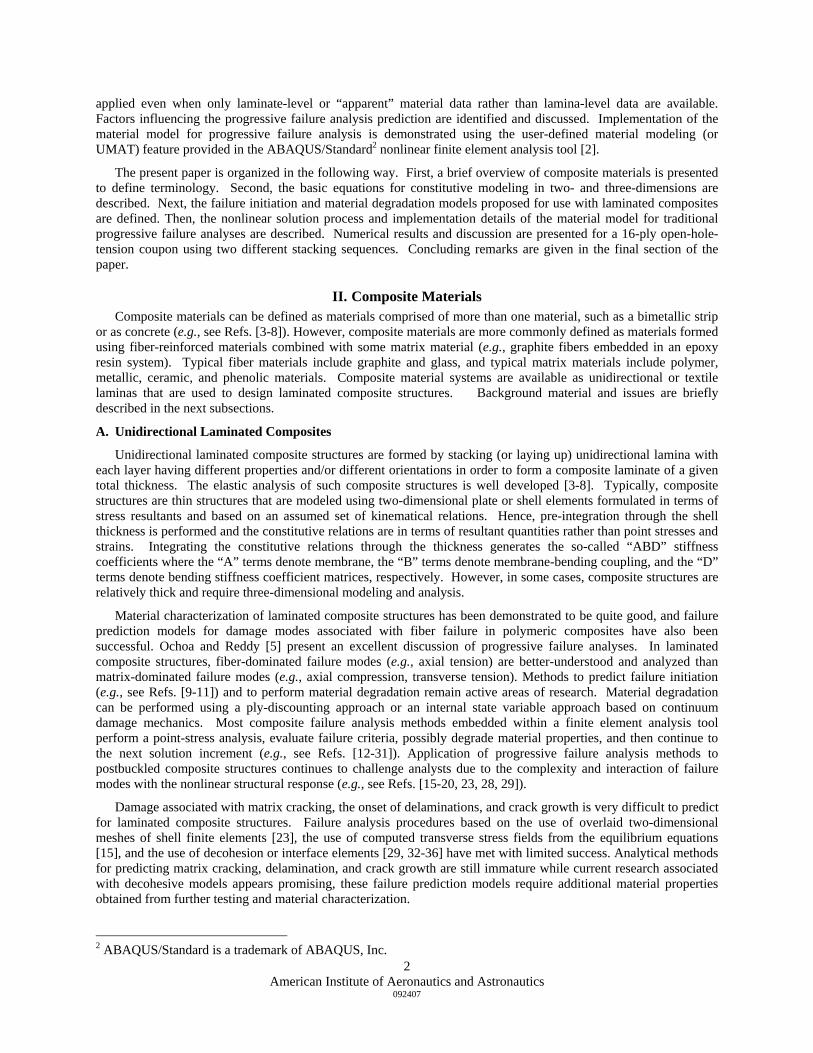
Progressive failure simulations are performed on the cross-ply open-hole-tension coupon using different failure criteria (different values of PDA). The applied tension load as a function of end displacement for different failure criteria are summarized in Figure 2 for two values of the maximum solution increment size. The short-dash line indicates the average failure load from three tests reported in Ref. [67]. The long-dash line represents the linear elastic response from the finite element analysis. Progressive failure analysis results were generated using the nominal lamina material data, a single integration point through the thickness of each lamina within the 16-ply laminate, and recursive degradation with a degradation factor β of 0.5. Results obtained using two different values of the maximum solution increment size factor for the nonlinear analysis are indicated in Figure 2 – 0.02 in Figure 2a and 0.01 in Figure 2b. For both values of this factor, overall the predicted progressive failure responses are similar. The maximum stress criteria (PDA=1) and the maximum strain criteria (PDA=2) predict nearly the same failure load (i.e., peak load) of approximately 11,200 pounds using the 0.02 value for the maximum solution increment size factor and approximately 9,500 pounds using the 0.01 value. The Tsai-Wu failure polynomial (PDA=3) predicts a lower failure load (10,300 pounds using the 0.02 value and 8,700 using the 0-.01 value) due the interactive nature of the failure criterion since the material system is a linear elastic brittle material. The Hashin criteria (PDA=4) under predict the failure load by nearly 30% due to the degradation model associated with tensile fiber failure, also referred to as fiber-matrix shear, see Eq. 7. As the maximum solution increment size factor is reduced, the peak load predictions obtained from the other failure criteria are reduced except for the Hashin criteria, which increased to 7,129 pounds. By reducing the maximum solution increment size, a smooth response is still predicted, and numerical drift in the simulation due to smaller solution increments is minimal.

The influence of the maximum increment size factor is shown in Figure 3a for the maximum strain criteria (PDA=2) and in Figure 3b for the Hashin criteria (PDA=4). Recursive degradation with a degradation factor β of 0.5 is used in all cases. Four values of the maximum increment size factor are considered. As the factor is reduced in size for the maximum strain criteria, the peak load prediction is also reduced as shown in Figure 3a. However, the load value corresponding to local fiber failure near the hole is the same for all values – approximately 7,000 pounds. For the Hashin criteria, the peak load predictions generally were unchanged with decreasing maximum solution increment size. However, for the smallest value considered (0.001), the peak load prediction is reduced by


092407

14

approximately 30%. The maximum solution increment size factor, which is used in the nonlinear solution strategy, apparently influences the post-ultimate behavior of the simulation, and its influence on the response needs to be established for each new analysis effort.

The influence of the degradation factor β is shown in Figure 4a for the maximum strain criteria (PDA=2) and in Figure 4b for the Hashin criteria (PDA=4). Recursive degradation and a maximum solution increment size factor of 0.02 are used in all cases. Five values of the degradation factor are considered for both criteria. As the degradation factor β is reduced, the peak load prediction for the maximum strain criteria is also reduced as indicated in Figure 4a; however, the load value corresponding to the initiation of local fiber failure near the hole is the same for all values of β. As the degradation factor β is reduced, the peak load prediction for the Hashin criteria is also reduced as indicated in Figure 4b. When recursive degradation is used, the degradation factor and the solution increment size have a combined effect on the predicted progressive failure response. For small values of the degradation factor, the local material stiffness coefficients degrade in value at a faster rate than when larger degradation factors are used and tend to simulate instantaneous degradation because of a near-zero degradation factor.

The influence of the maximum solution increment size factor is shown in Figure 5 for the maximum strain criteria (PDA=2) using instantaneous degradation with a degradation factor β of 10-6. Three values of the maximum increment size factor are considered. As the factor is reduced, the peak load prediction is essentially the same as the peak load predicted using recursive degradation with a degradation factor of 0.001. Reducing the maximum solution increment size factor has little effect on the progressive failure response prediction when using instantaneous degradation with a very small value of the degradation factor (i.e., β=10-6).

Peak failure loads are summarized in Table 1 for different failure criteria using recursive degradation with a degradation factor β of 0.5 and a maximum increment size factor of 0.01. The maximum stress (PDA=1) and maximum strain (PDA=2) criteria give essentially the same result since the material is a linear elastic brittle material, and these predicted failure loads correlate well with the reported average test value [67]. The Tsai-Wu failure polynomial (PDA=3) predicts a similar behavior and onset of damage; however, a lower failure load is predicted. The Hashin criteria (PDA=4) under predict the peak load by nearly 25%.

Progressive failure simulations performed on the cross-ply open-hole-tension coupon using different failure criteria are also performed using the apparent or smeared material properties for the cross-ply laminate given in the appendix. These progressive failure analysis results are generated using the effective engineering material data, three integration points through the laminate thickness, and recursive degradation with a degradation factor β of 0.5. The maximum solution increment size factor is 0.01 for the nonlinear analysis. The results obtained using the effective material data are shown in Table 1 and are consistent with the results obtained using the cross-ply laminate (ply-by-ply) modeling approach with a single integration point in each layer. However, information on individual lamina failure modes is not recoverable when the effective properties and laminate modeling approach is used. In addition, results generated for the case of a single integration point through the laminate thickness agree with those generated using only three integration points for this example problem.

Progressive failure simulations performed on the quasi-isotropic open-hole-tension coupon using different failure criteria are summarized in Figure 6. The short-dash line indicates the average failure load from two tests [67]. The long-dash line represents the linear elastic response from the finite element analysis. These progressive failure analysis results are generated using the nominal lamina material data, a single integration point through the thickness of each lamina, recursive degradation with a degradation factor β of 0.5, and a maximum solution increment size factor of 0.01. The maximum stress (PDA=1) and maximum strain (PDA=2) criteria again give essentially the same result because the material is a linear elastic brittle material. The Tsai-Wu failure polynomial (PDA=3) predicts a similar behavior and failure load since the laminate is quasi-isotropic. The Hashin criteria (PDA=4) under predict the peak load. This lower peak load prediction by the Hashin criteria is due to the tensile fiber failure mode defined in Eq. 7 and its associated degradation rules. Alternate failure criteria and degradation rules are given by Chang et al. [67]; however, they are not included in the current version of this UMAT subroutine [1].

The predicted peak failure loads for the open-hole-tension coupons are summarized in Table 1. For the cross-ply laminate case, the peak failure loads predicted by the maximum stress, maximum strain, and Tsai-Wu criteria are within 10% of the average failure load from test. The Hashin criteria gave very conservative predictions (lower by more than 25%). Similar trends are obtained for the cross-ply case using smeared or apparent material data. For the quasi-isotropic laminate case, the peak failure loads predicted by the maximum stress, maximum strain, and Tsai-


092407

15

Wu criteria are within 2% of the average failure load from test. The Hashin criteria again gave conservative predictions (lower by 23%).

IX. Concluding Remarks A user-defined material model for laminated composite structures is described in the present paper. This

material model takes advantage of previous work in progressive failure analysis of laminated polymeric composites. In addition, extensions of these models are provided for bimodulus materials. Progressive failure analysis options are provided for different point-stress methods with traditional failure initiation and material degradation models as well as from a linear elastic model. These models are implemented within an UMAT subroutine and are executed using the ABAQUS/Standard nonlinear finite element tool.

Each of the progressive failure analysis models is summarized in the present paper and fully described in Ref. [1]. For the ply-discounting models, the failure initiation criteria are described as well as the procedure for material degradation. Material degradation is achieved through a set of degradation factors dependent on whether the failure mode is tension, compression or shear driven. Material degradation is applied to the material stiffness coefficients rather than the elastic engineering mechanical properties to maintain symmetry in the local material stiffness matrix. Material degradation can be applied instantaneously or recursively in the ply-discounting models. Recursive degradation in combination with fractional degradation factors is found to provide reliable progressive failure solutions.

The features of the progressive failure analysis models implemented in this UMAT subroutine are illustrated using two 16-ply open-hole-tension coupons. One coupon has a cross-ply lamination scheme, and the other coupon has a quasi-isotropic lamination scheme. This material exhibited a linear elastic orthotropic brittle behavior. The form of degradation, the degradation factor, and the solution increment size are found to influence the progressive failure predictions. The maximum stress and maximum strain criteria predicted nearly the same peak failure loads and nonlinear response. While the Tsai-Wu failure polynomial criterion predicted lower peak failure loads, these predictions are still in good agreement with test results. The Hashin criteria typically under predicted the peak failure loads by approximately 25% for a nominal value of the degradation factor (β=0.5) when combined with recursive degradation. This result is tied to the material degradation model for the tensile fiber failure mode given by Eq. 7. This expression typically implies a fiber-matrix shear failure, and material degradation should only be applied to the in-plane shear coefficients [67]. However, typical material degradation implementations associated with the Hashin criteria, including the present UMAT subroutine, degrade the in-plane normal coefficients as well as the in-plane shear term when this failure mode is detected, which leads to a conservative failure prediction.


092407

16

Appendix The UMAT material property data for a representative T800/3900-2 graphite epoxy composite material [67]

named T800H39002 are defined using the following records:

** UMAT Property Data Definitions ** props(1-8):E11t,E22t,E33t,E11c,E22c,E33c,G12,G13, ** props(9-16):G23,nu12,nu13,nu23, Xt, Yt, Zt, Xc, ** props(17-24):Yc,Zc,S12,S13,S23,Eps11T,Eps22T,Eps33T, ** props(25-32):Eps11C,Eps22C,Eps33C,Gam12,Gam13,Gam23,Eps11Tmx,Eps22Tmx, ** props(33-40):Eps33Tmx,Eps11Cmx,Eps22Cmx,Eps33Cmx,Gam12mx,Gam13mx,Gam23mx,GIc, ** props(41-48):FPZ,SlimT,SlimC,SlimS,weibull(1),weibull(2),weibull(3),weibull(4), ** props(49-55):weibull(5),weibull(6),Dgrd(1),Dgrd(2),Dgrd(3),RECURS,PDA ** ========================================================================================== ** T300H/3900-2 Material 1 with total thickness = 0.00645 inches per ply *MATERIAL, NAME=T800H39002 *USER MATERIAL, CONSTANTS=55 2.320E+07, 1.300E+06, 1.300E+06, 2.320E+07, 1.300E+06, 1.300E+06, 0.900E+06, 0.900E+06, 0.500E+06, 2.800E-01, 2.800E-01, 2.800E-01, 4.120E+05, 8.720E+03, 8.720E+03, 2.250E+05, 2.430E+04, 2.430E+04, 1.376E+04, 1.376E+04, 7.644E+03, 0.178E-01, 0.671E-02, 0.671E-02, 0.970E-02, 0.187E-01, 0.187E-01, 0.153E-01, 0.153E-01, 0.153E-01, 1.000E-01, 1.000E-01, 1.000E-01, 1.000E-01, 1.000E-01, 1.000E-01, 1.000E-01, 1.000E-01, 1.000E-01, 0.860E+00, 2.000E-01, 0.800E+00, 0.800E+00, 0.800E+00, 1.000E+00, 1.000E+00, 1.000E+00, 1.000E+00, 1.000E+00, 1.000E+00, 5.000E-01, 5.000E-01, 5.000E-01, 1.000E+00, 4.000E+00 *DEPVAR 8 Note that the only difference for applying this UMAT subroutine to two-dimensional or three-dimension problems is the last keyword *DEPVAR. This keyword defines the number of solution-dependent variables or SDVs for the problem. For two-dimensional finite elements, it is 8, and for three-dimensional finite elements, it is 14.

For the present 16-ply cross-ply laminate, the effective engineering properties were calculated and used as the “apparent” mechanical properties for the entire 16-ply laminate. The input records for the UMAT subroutine based on smeared or effective engineering properties of this system are: ** UMAT Property Data Definitions ** props(1-8):E11t,E22t,E33t,E11c,E22c,E33c,G12,G13, ** props(9-16):G23,nu12,nu13,nu23, Xt, Yt, Zt, Xc, ** props(17-24):Yc,Zc,S12,S13,S23,Eps11T,Eps22T,Eps33T, ** props(25-32):Eps11C,Eps22C,Eps33C,Gam12,Gam13,Gam23,Eps11Tmx,Eps22Tmx, ** props(33-40):Eps33Tmx,Eps11Cmx,Eps22Cmx,Eps33Cmx,Gam12mx,Gam13mx,Gam23mx,GIc, ** props(41-48):FPZ,SlimT,SlimC,SlimS,weibull(1),weibull(2),weibull(3),weibull(4), ** props(49-55):weibull(5),weibull(6),Dgrd(1),Dgrd(2),Dgrd(3),RECURS,PDA ** ========================================================================================== ** T800H/3900-2 graphite epoxy with 0.00645 inches per ply ** Smeared laminate values based on effective engineering properties Ex and Ey ** for the [(0/90)_4]_s laminate *MATERIAL, NAME=SMEARED16 *USER MATERIAL, CONSTANTS=55 1.229E+07, 1.229E+07, 1.300E+06, 1.229E+07, 1.229E+07, 1.300E+06, 0.900E+06, 0.900E+06, 0.500E+06, 2.970E-02, 2.970E-02, 2.970E-02, 2.104E+05, 2.104E+05, 8.720E+03, 1.247E+05, 1.247E+05, 2.430E+04, 1.376E+04, 1.376E+04, 7.644E+03, 0.171E-01, 0.171E-01, 0.671E-02, 0.101E-01, 0.101E-01, 0.187E-01, 0.153E-01, 0.153E-01, 0.153E-01, 1.000E-01, 1.000E-01, 1.000E-01, 1.000E-01, 1.000E-01, 1.000E-01, 1.000E-01, 1.000E-01, 1.000E-01, 0.860E+00, 2.000E-01, 0.000E+00, 0.000E+00, 0.000E+00, 1.000E+00, 1.000E+00, 1.000E+00, 1.000E+00, 1.000E+00, 1.000E+00, 5.000E-01, 5.000E-01, 5.000E-01, 1.000E+00, 3.000E+00 *DEPVAR 8


092407

17

References 1. Knight, N. F., Jr., User-Defined Material Model for Progressive Failure Analysis, NASA CR-2006-214526,

December 2006.

2. Anon., ABAQUS/Standard User’s Manual, Version 6.5, ABAQUS, Inc., Providence, RI, 2004.

3. Jones, Robert M., Mechanics of Composite Materials, McGraw-Hill Book Company, New York, 1975. Second Edition, Taylor and Francis, Philadelphia, PA, 1999.

4. Tsai, Stephen W. and Hahn, H. Thomas, Introduction to Composite Materials, Technomic Publishers, Westport, CN, 1980.

5. Ochoa, O. and Reddy, J. N., Finite Element Analysis of Composite Laminates, Kluwer Academic Publishers, Dordrecht, The Netherlands, 1992.

6. Hyer, Michael H., Stress Analysis of Fiber-Reinforced Composite Materials, McGraw-Hill, Boston, 1998.

7. Herakovich, Carl T., Mechanics of Fibrous Composites, John Wiley and Sons, New York, 1998.

8. Kelly, A. and Zweben, C. (editors), Comprehensive Composite Materials, Elsevier Science Ltd., 2000.

9. Tsai, S. W. and Wu, E. M., “A General Theory of Strength for Composite Anisotropic Materials,” Journal of Composite Materials, Vol. 5, January 1971, pp. 58-80.

10. Rosen, B. W. and Zweben, C. H., Tensile Failure Criteria for Fiber Composite Materials, NASA CR-2057, August 1972.

11. Hashin, Z. “Failure Criteria for Unidirectional Fiber Composites,” ASME Journal of Applied Mechanics, Vol. 47, No. 2, June 1980, pp. 329-334.

12. Lee, J. D., “Three Dimensional Finite Element Analysis of Damage Accumulation in Composite Laminate,” Computers and Structures, Vol. 15, No. 3, 1982, pp. 335-350.

13. Ochoa, O. O. and Engblom, J. J., “Analysis of Failure in Composites,” Composites Science and Technology, Vol. 28, 1987, pp. 87-102.

14. Chang, F. K. and Chang, K. Y., “A Progressive Damage Model for Laminated Composites Containing Stress Concentrations,” Journal of Composite Materials, Vol. 21, No. 9, 1987, pp. 834-855.

15. Engelstad, S. P., Reddy, J. N., and Knight, N. F., Jr., “Postbuckling Response and Failure Prediction of Graphite-Epoxy Plates Loaded in Compression,” AIAA Journal, Vol. 30, No. 8, August 1992, pp. 2106-2112.

16. Krishna Murty, A.V. and Reddy, J. N., “Compressive Failure of Laminates and Delamination Buckling: A Review,” The Shock and Vibration Digest, Vol. 25, No. 3, March 1993, pp. 3-12.

17. Reddy, Y. S. and Reddy, J. N., “Three-Dimensional Finite Element Progressive Failure Analysis of Composite Laminates under Axial Compression,” Journal of Composite Technology and Research, Vol. 15, No. 2, Summer 1993, pp. 73-87.

18. Singh, S. B., Kumar, A., and Iyengar, N. G. R., “Progressive Failure of Symmetrically Laminated Plates under Uni-axial Compression,” Structural Engineering and Mechanics, Vol. 5, No. 4, 1997, pp. 433-450.

19. Sleight, D. W., Knight, N. F., Jr., and Wang, J. T., “Evaluation of a Progressive Failure Analysis Methodology for Laminated Composite Structures,” AIAA Paper No. 97-1187, presented at the AIAA/ASME/ASCE/AHS/ASC 38th Structures, Structural Dynamics, and Materials Conference, Kissimmee, FL, April 7-10, 1997.

20. Moas, E. and Griffin, O. H., Jr., “Progressive Failure Analysis of Laminated Composite Structures,” AIAA Paper No. 97-1186, presented at the AIAA/ASME/ASCE/AHS/ASC 38th Structures, Structural Dynamics, and Materials Conference, Kissimmee, FL, April 7-10, 1997.

21. Soden, P. D., Hinton, M. J., and Kaddour, A. S., “A Comparison of the Predictive Capabilities of Current Failure Theories for Composite Structures,” Composite Science and Technology, Vol. 58, 1998, pp. 1225-1254.


092407

18

22. Huybrechts, S., “Failure of Composite Structures,” in Advances in Composite Materials and Mechanics, Arup Maji (editor), ASCE, 1999, pp. 34-41.

23. Dávila, C. G., Ambur, D. R., and McGowan, D. M., “Analytical Prediction of Damage Growth in Notches Composite Panels Loaded in Compression,” Journal of Aircraft, Vol. 37, No. 5, September-October 2000, pp. 898-905.

24. Barbero, E. J. and Lonetti, P., “An Inelastic Damage Model for Fiber Reinforced Laminates,” Journal of Composite Materials, Vol. 36, No. 8, 2002, pp. 941-962.

25. Lin, W.-P. and Hu, H.T., “Nonlinear Analysis of Fiber-Reinforced Composite Laminates Subjected to Uniaxial Tensile Load,” Journal of Composite Materials, Vol. 36, No. 12, 2002, pp. 1429-1450.

26. Lin, W.-P. and Hu, H.T., “Parametric Study on the Failure of Fiber-Reinforced Composite Laminates under Biaxial Tensile Load,” Journal of Composite Materials, Vol. 36, No. 12, 2002, pp. 1481-1503.

27. Huybrechts, S., Maji, A., Lao, J., Wegner, P., and Meink, T., “Validation of the Quadratic Composite Failure Criteria with Out-of-Plane Shear Terms,” Journal of Composite Materials, Vol. 36, No. 15, 2002, pp. 1879-1888.

28. Knight, N. F., Jr., Rankin, C. C., and Brogan, F. A., “STAGS Computational Procedure for Progressive Failure Analysis of Laminated Composite Structures,” International Journal of Non-Linear Mechanics, Vol. 37, No. 4-5, 2002, pp. 833-849.

29. Goyal, V. K., Jaunky, N., Johnson, E. R., and Ambur, D. R., “Intralaminar and Interlaminar Progressive Failure Analyses of Composite Panels with Circular Cutouts,” AIAA Paper No. 2002-1745, presented at the AIAA/ASME/ASCE/AHS/ASC 43rd Structures, Structural Dynamics, and Materials Conference, Denver, CO, April 22-25, 2002.

30. Hinton, M. J., Kaddour, A. S., and Soden, P. D. (editors), Failure Criteria in Fibre-Reinforced-Polymer Composites: The World-Wide Failure Exercise, Elsevier Science Publishing Company, Oxford, 2004.

31. Dávila, C. G., Camanho, P. P., and Rose, C. A., “Failure Criteria for FRP Laminates,” Journal of Composite Materials, Vol. 39, No. 4, February 2005, pp. 323-345.

32. Shahwan, K. W. and Waas, A. M., “Non-Self-Similar Decohesion along a Finite Interface of Unilaterally Constrained Delaminations,” Proceedings of the Royal Society of London, Series A: Mathematical, Physical and Engineering Sciences, Vol. 453, Issue 1958, March 8, 1997, pp. 515-550.

33. Chen, J., Crisfield, M., Kinloch, A. J., Busso, E. P., Matthews, F. L., and Qiu, Y., “Predicting Progressive Delamination of Composite Material Specimens via Interface Elements,” Mechanics of Composite Materials and Structures, Vol. 6, No. 4, Oct.-Dec. 1999, pp. 303-317.

34. Camanho, P. P., Dávila, C. G., and Ambur, D. R., Numerical Simulation of Delamination Growth in Composite Materials, NASA TP 2001-211041, August 2001.

35. Dávila, C. G., Camanho, P. P., and de Moura, M. F., “Mixed-Mode Decohesion Elements for Analyses of Progressive Delamination,” AIAA Paper No. 2001-1486, presented at the AIAA/ASME/ASCE/AHS/ASC 42nd Structures, Structural Dynamics, and Materials Conference, Seattle, WA, April 16-19, 2001.

36. Goyal, V. K., Analytical Modeling of the Mechanics of Nucleation and Growth of Cracks, Ph. D. Dissertation, Department of Aerospace and Ocean Engineering, Virginia Polytechnic Institute and State University, Blacksburg, VA, December 2002.

37. Ishikawa, T. and Chou, T.-W., “Stiffness and Strength Behaviour of Woven Fabric Composites,” Journal of Material Science, Vol. 17, 1982, pp. 3211-3220.

38. Raju, I. S. and Wang, J. T., “Classical Laminate Theory Models for Woven Fabric Composites,” Journal of Composites Technology and Research, Vol. 16, No. 4, October 1994, pp. 289-303.

39. Naik, R. A., “Failure Analysis of Woven and Braided Fabric Reinforced Composites,” Journal of Composite Materials, Vol. 29, No. 17, 1995, pp. 2334-2363.


092407

19

40. Poe, C. C., Jr. and Harris, C. E. (editors), Mechanics of Textile Composites Conference, NASA CP-3311, Parts 1 and 2, October 1995.

41. Cox, B., Failure Models for Textile Composites, NASA CR-4686, August 1995.

42. Cox, B. and Flanagan, G., Handbook of Analytical Methods for Textile Composites, NASA CR-4750, March 1997.

43. Poe, C. C., Jr., Dexter, H. B., and Raju, I. S., “Review of the NASA Textile Composites Research,” Journal of Aircraft, Vol. 36, No. 5, September-October 1999, pp. 876-884.

44. Schwer, L. E. and Whirley, R. G., “Impact of a 3D Woven Textile Composite Thin Panel: Damage and Failure Modeling,” Mechanics of Composite Materials and Structures, Vol. 6, No. 1, 1999, pp. 9-30.

45. Hahn, H. T., “Nonlinear Behavior of Laminated Composites,” Journal of Composite Materials, Vol. 7, No. 2, April 1973, pp. 257-271.

46. Hahn, H. T., “A Note on Determination of the Shear Stress-Strain Response of Unidirectional Composites,” Journal of Composite Materials, Vol. 7, No. 3, July 1973, pp. 383-386.

47. Whitney, J. M., “Shear Correction Factors for Orthotropic Laminates under Static Load,” ASME Journal of Applied Mechanics, Vol. 40, March 1973, pp. 302-304.

48. Ambartsumyan, S. A., “The Basic Equations and Relations of the Different-Modulus Theory of Elasticity of an Anisotropic Body,” Mechanics of Solids, Vol. 4, No. 3, 1969, pp. 48-56. Originally in Russian in Akademiia Nauk SSSR, Izvestiia, Mekhanika Tverdogo Tela, Vol. 4, No. 3, pp. 51-61, 1969.

49. Tabaddor, F., “Constitutive Equations for Bimodulus Elastic Materials,” AIAA Journal, Vol. 10, No. 4, April 1972, pp. 516-518.

50. Jones, R. M., “Stress-Strain Relations for Materials with Different Moduli in Tension and Compression,” AIAA Journal, Vol. 15, No. 1, January 1977, pp. 16-23.

51. Bert, C. W., “Models for Fibrous Composites with Different Properties in Tension and Compression,” ASME Journal of Engineering Materials and Technology, Vol. 99, No. 4, October 1977, pp. 344-349.

52. Reddy, J. N. and Chao, W. C., “Finite-Element Analysis of Laminated Bimodulus Composite-Material Plates,” Computers and Structures, Vol. 12, 1980, pp. 245-251.

53. Vijayakumar, K. and Rao, K. P., “Stress-Strain Relations for Composites with Different Stiffnesses in Tension and Compression,” Computational Mechanics, Vol. 2, No. 3, 1987, pp. 167-175.

54. Krajcinovic, D., “Continuum Damage Mechanics,” Applied Mechanics Reviews, Vol. 37, No. 1, January 1984, pp. 1-6.

55. Lemaitre, J., “How to Use Damage Mechanics,” Nuclear Engineering and Design, Vol. 80, 1984, pp. 233-245.

56. Talreja, R., “Modeling of Damage Development in Composites using Internal Variable Concepts,” in Damage Mechanics in Composites, A. S. D. Wang and G. K. Haritos (editors), ASME AD-Vol. 12, 1987, pp. 11-16.

57. Ladevèze, P. and LeDantec, E., “Damage Modeling of the Elementary Ply for Laminated Composites,” Composites Science and Technology, Vol. 43, 1992, pp. 257-267.

58. Shahid, I. and Chang, F.-K., “Accumulative Damage Model for Tensile and Shear Failures of Laminated Composite Plates,” Journal of Composite Materials, Vol. 29, No. 7, July 1995, pp. 926-981.

59. Krajcinovic, D., Damage Mechanics, North Holland Publishing, Amsterdam, 1996.

60. Matzenmiller, A., Lubliner, J., and Taylor, R. L., “A Constitutive Model for Anisotropic Damage in Fiber-Composites,” Mechanics of Materials, Vol. 20, No. 2, April 1995, pp. 125-152.

61. Weibull, W., “A Statistical Distribution Function of Wide Applicability,” ASME Journal of Applied Mechanics, Vol. 18, September 1951, pp. 293-297.


092407

20

62. Creasy, T. S., “Modeling Analysis of Tensile Tests of Bundled Filaments with a Bimodal Weibull Survival Function,” Journal of Composite Materials, Vol. 36, No. 2, 2002, pp. 183-194.

63. Hahn, H. T. and Tsai, S. W., “On the Behavior of Composite Laminates after Initial Failures,” Journal of Composite Materials, Vol. 8, July 1974, pp. 288-305.

64. Petit, P. H. and Waddoups, M. E., “A Method of Predicting the Nonlinear Behavior of Laminated Composites,” Journal of Composite Materials, Vol. 3, January 1969, pp. 2-19.

65. Schweizerhof, K., Weimer, K., Münz, Th., and Rottner, Th., “Crashworthiness Analysis with Enhanced Composite Material Models in LS-DYNA – Merits and Limits,” in Proceedings of the 5th International LS-DYNA Users Conference, Southfield, MI, September 21-22, 1998.

66. Anon., LS-DYNA Users Manual – Volume II (Material Models, References and Appendices), Version 960, Livermore Software Technology Corporation, Livermore, CA, March 2001.

67. Chang, F.-K., Qing, X., Sun, H.-T., and Yan, Y., Damage Tolerance-Based Design of Bolted Composite Joints, Final Report under Contract No. TZ-370444-07LHN, Department of Aeronautics and Astronautics, Stanford University, 2000.

Table 1. Summary of the peak failure loads for the cross-ply and quasi-isotropic 16-layer graphite-epoxy open-hole-

tension coupons using different failure criteria, a maximum solution increment size of 0.01, and recursive degradation with a degradation factor β of 0.5.

Peak Failure Load, pounds

Progressive

Failure

Analysis

(value of PDA)

Cross-ply

(laminate)

Cross-ply

(smeared)

Quasi-

isotropic

(laminate)

Max. Stress (1) 9,531 10,041 7,975

Max. Strain (2) 9,620 9,996 7,941

Tsai-Wu (3) 8,655 9,466 7,869

Hashin (4) 7,129 6,056 5,985

Test Average

[67]

9,605 9,605 7,810


092407

21

(a) Complete model. (b) Close-up view of region near the hole.

Figure 1. Finite element model of the open-hole-tension coupon.


092407

22

(a) Predictions obtained using a 0.02 value for the maximum solution increment size.

(b) Predictions obtained using a 0.01 value for the maximum solution increment size.

Figure 2. Comparison of different progressive failure analysis models for the 16-ply cross-ply open-hole-tension coupon using recursive degradation with a degradation factor β of 0.5.


092407

23

(a) Results using maximum strain criteria (PDA=2).

(b) Results using Hashin criteria (PDA=4).

Figure 3. Influence of maximum solution increment size on the progressive failure predictions for the 16-ply cross-ply open-hole-tension coupon using recursive degradation with a degradation factor β of 0.5.


092407

24

(a) Results using maximum strain criteria (PDA=2).

(b) Results using Hashin criteria (PDA=4).

Figure 4. Influence of degradation factor β on the progressive failure predictions for the 16-ply cross-ply open-hole-tension coupon using recursive degradation and a maximum solution increment size of 0.02.


092407

25

Figure 5. Influence of maximum solution increment size on the progressive failure predictions for the 16-ply cross-

ply open-hole-tension coupon using the maximum strain criteria (PDA=2) and instantaneous degradation with a degradation factor β of 10-6.

Figure 6. Comparison of different progressive failure analysis models for the 16-ply quasi-isotropic open-hole-

tension coupon using recursive degradation with a degradation factor β of 0.5 and a maximum solution increment size of 0.01.

factors influencing progressive failure analysis predictions for laminated composite ... · ·...

Documents