use power series for solve differential equations
TRANSCRIPT
Ministry of Higher Education
and Scientific Research
University of Al-Qadisiyha
College of Education
A Research
Submitted to the College Education of University of Al-
Qadisiyha in partial fulfillment of the erquirements for the
Degree of Bachelor's in Mathematies
By
Huda Kadhem Abied
Supervised by
Asst .Dr. Khalid MINDEEL AL – Abraheme
2019AD 1440AH
Use power series for solve differential equations

الرحيم الرحمن الله بسم
(قليلا الا العلم من وأوتيتم)
العظيم العلي الله صدق

Dedication
To…..
My dear father .
My compassionate mother .
My brother and sisters .
My husband.

الشكر و التقدير
بعد شكري لـلـه عز وجل أن أعانني على انجاز هذا البحث المتواضع اتقدم بجزيل الشكر
على تفضله بقبول الاشراف على خالد منديل الإبراهيمي والامتنان الى الاستاذ الفاضل الدكتور
س المنير في كل ابحثي هذا، وعلى ما اسداه لي من نصائح وارشادات كانت بمثابة النبر
.خطواتي يفوتني بهذه المناسبة ان اوجه شكري واحترامي الى كل من ساعدني من قريب او ولا
اختي العزيزة زهراء متواضع، واخص بالذكر بعيد في انجاز هذا الجهد ال

Supervisor is Certification
Certify that the research entitled "Use power series for solve differential equations" ,was
prepared by " Huda Kadhem Abied" under my supervision at Baghdad University ,College of
Science , Department of Mathematics as a partial fulfillment of the requirements for the
degree of Doctor of Philosophy in Mathematics.
Signature:
Name : Khalid Mindeel Al- Abraheme
Title:
Date : / / 2019

Abstract
In this paper we in traduce New method for
solve ordinary differential equation by power
series and compare this method withe some of
method We have compared the proposed
method with some traditional methods and
found our method followed by a more accurate,
faster and less error ratio

contents Tvo.page
Contents
Chapter 1 : Background
1-1 Background
1-2 Hinger order equations
1-3 Numerical Solution
1-4 Initial – Value Problems For Ordinary
Differential Equations
Chapter 2 : Using power Series to Solve
Differential Equations
2-1 Using power Series to Solve Differential
Equations
2-2 Examples
1
5
6
7
13
13

Chapter 1
Background

Chapter one Background
1. 1- Background
Many ordinary differential equations encountered do not have easily obtain able closed
from solutions , and we must seek other methods by which solutions can be constructed .
Numerical methods provide an alternative way of constructing solutions to these some times
difficult problems . In this chapter we present an introduction to some numerical methods which
can be applied to awide variety of ordinary differential equations . These methods can be
programmed into a digital computer or even programmed into some hand – held calculators .
Many of the numerical techniques introduced in this chapter are readily available in the from of
subroutine packages available from the internet .
An equation that consists of derivatives is called a differential equation .
Differential equations have applications in all areas of science and engineering .
Mathematical formulation of most of the physical and engineering problems lead to differential
equations .
So , it is important for engineers and scientists to know how to set up differential equations and
solve them .
Differential equations are of two types ordinary differential equation " ODE " and partial
differential equations "PDE" .

Chapter one Background
An ordinary differential equation is that in which all the derivatives are with respect to a single
independent variable . Examples of ordinary differential equation include .
1- 4y(0) , 2)0(dx
dy , 0y
dx
dy2
dx
yd2
2
.
2- 4y(0) , 12)0(dx
yd sin x y
dx
dy5
dx
yd3
dx
yd2
2
2
2
3
3
4y(0) , 2)0(dx
dy
Note : In this first part , we will see how to solve ODE of the form.
0yy(0) , y)f(x,dx
dy
In another sextion , we will discuss how to solve higher ordinary differential equations
or coupled "simultaneous" differential equations .
But first , How to write a first order differentia
Equation for example

Chapter one Background
5y(0) , 1.3e2ydx
dy x-
Is rewritten as :
5y(0) ,2y -1.3edx
dy x-
Is this case : y21.3ey)f(x, x
Example (2) : 5y(0) , 2sin(3x)yxdx
dye 2y
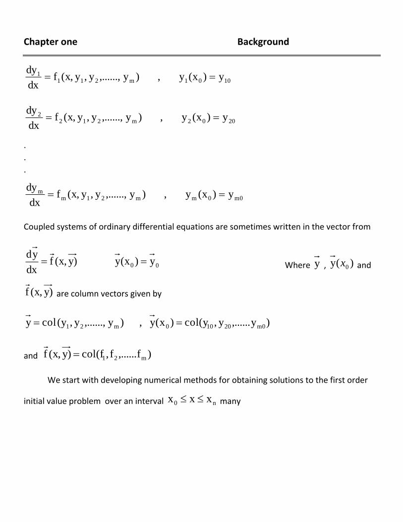
We consider the problem of developing numerical methods to solve a first order initial
value problem of the form.
00 y)y(x , y)f(x,dx
dy
and then consider how to generalize these methods to solve systems of ordinary differential
equations having the form .
Chapter one Background
1001m2111 y)(xy , )y,......,y,y(x,f
dx
dy
2002m2122 y)(xy , )y,......,y,y(x,f
dx
dy
.
.
.
m00mm21mm y)(xy , )y,......,y,y(x,f
dx
dy
Coupled systems of ordinary differential equations are sometimes written in the vector from
00 y)(xy y)(x,fdx
yd Where y , )(y 0x and
y)(x,f are column vectors given by
)y,......y,col(y)x(y , )y,......,y,(y coly m020100m21
and )f,......f,col(fy)(x,f m21
We start with developing numerical methods for obtaining solutions to the first order
initial value problem over an interval n0 xxx many
Chapter one Background
of the techniques developed for this first order equation can with modifications , also be
applied to solve a first order system of differential equations.
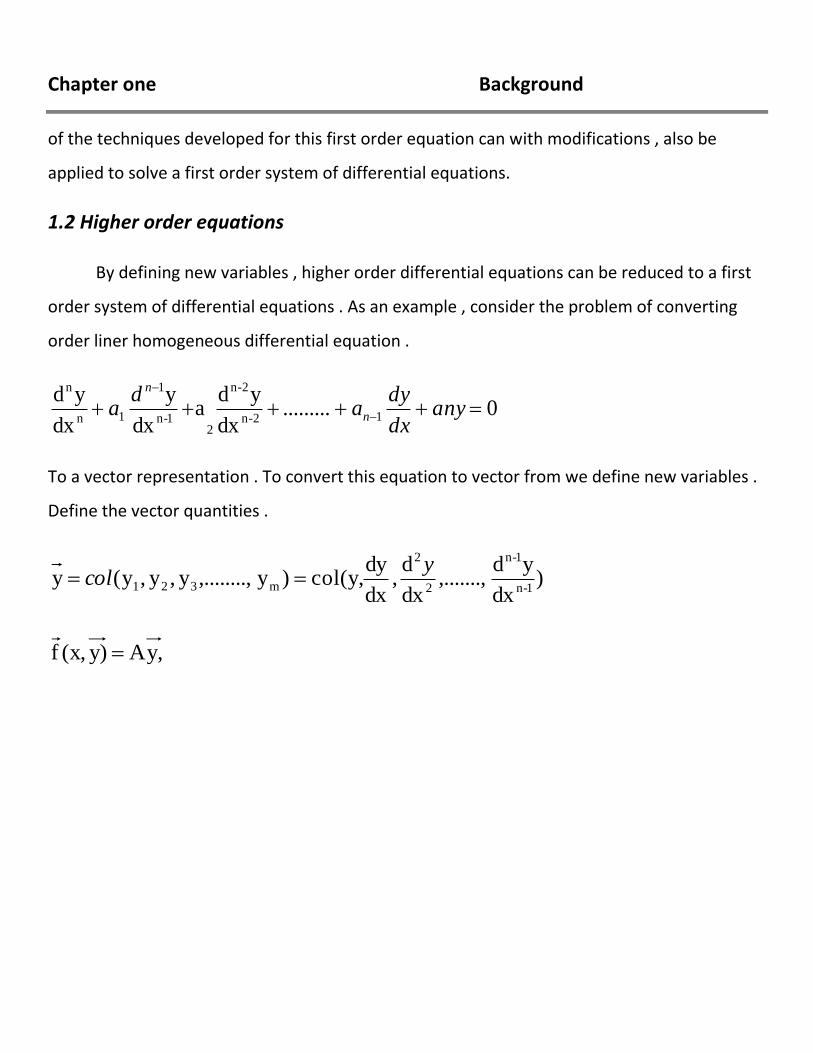
1.2 Higher order equations
By defining new variables , higher order differential equations can be reduced to a first
order system of differential equations . As an example , consider the problem of converting
order liner homogeneous differential equation .
0.........dx
yda
dx
y
dx
yd12-n
2-n
21-n
1
1n
n
anydx
dya
da n
n
To a vector representation . To convert this equation to vector from we define new variables .
Define the vector quantities .
)dx
yd,.......,
dx
d,
dx
dycol(y,)y,........,y,y,y(y
1-n
1-n
2
2
m321
ycol
y,Ay)(x,f
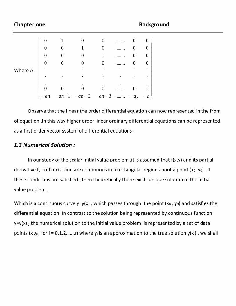
Chapter one Background
Where A =
12........321
10........0000
.
.
.
.
.
.
.
.
.
.
.
.
.
.
.
.
.
.
.
.
.00........0000
00........1000
00........0100
00........0010
aaanananan
Observe that the linear the order differential equation can now represented in the from
of equation .In this way higher order linear ordinary differential equations can be represented
as a first order vector system of differential equations .
1.3 Numerical Solution :
In our study of the scalar initial value problem .it is assumed that f(x,y) and its partial
derivative fy both exist and are continuous in a rectangular region about a point (x0 ,y0) . If
these conditions are satisfied , then theoretically there exists unique solution of the initial
value problem .
Which is a continuous curve y=y(x) , which passes through the point (x0 , y0) and satisfies the
differential equation. In contrast to the solution being represented by continuous function
y=y(x) , the numerical solution to the initial value problem is represented by a set of data
points (xi,yi) for i = 0,1,2,…..,n where yi is an approximation to the true solution y(xi) . we shall

Chapter one Background
investigate various methods for constructing the data points (xi,yi) , for i=1,2,…,n which
approximate the true solution to the given initial value problem . The given rule or technique
used to obtain the numerical solution is called anumerical method or algorithm . There are
many numerical methods for solving ordinary differential equations . In this chapter we will
consider only a select few of the mor popular methods . The numerical methods considered
can be classified as either single – step methods or multi-step methods . We begin our
introduction to numerical methods for ordinary differential
equations by considering single step methods .
1.4 Initial – Value Problems For Ordinary Differential Equations
Many problems in engineering and science can be formulated in terms of differential
equations . A differential equation is an equation involving a relation between an un known
function and one or more of its derivatives . Equations involving derivatives of only one
independent variable are called ordinary differential equations and may be classified as either
initial – value problems " IVP " or boundary value problems "BVP" . Examples of the two types
are :
-yxy:IVP

Chapter one Background
Y(0) = 2 , 1(0)y
-yxy : BVP
Y(0) = 2 , y(1) = 1
Where the prime denotes differentiation with respect to x. The distinction between the two
classifications lies in the location where the extra conditions are specified . For an IVP , the
conditions are given at the same value of , where as in the case of the BVP , They are
prescribed at two different values of x .
Since there are relatively few differential equations arising from practical problems for
which anal arising from practical problems for which analytical solutions are known , one must
resort to numerical methods . In this situation it turns out that the numerical methods for each
type of problem , IVP or BVP , are quite different and require separate treatment . In this
chapter we discuss .
Consider the problem of solving the mth-order differential equation .
conditions initial with ),...,,,(y )1((m) myyyxf

Chapter one Background
1)-(m
00
1)-(m
00
00
y)x(y
.
.
.
y)(xy
y)y(x
Where f is known function and 1)-(m
000 y,........,y,y are constants . It is customary to
rewrite as an equivalent system of m first – order equations . To do so , we define a new set of
dependent variables y(x) , y2(x) , ……. , ym(x) by :
1)-(m
m
3
2
1
yy
.
.
.
yy
yy
y
y
And transform into :

Chapter one Background
)y,.......,y,yfm(x,)y,,.........y,yf(x,y
.
.
(1.5) .
)y,,.........y,yx,(f yy
)y.,,.........y,yx,(f yy
m21m21m
m21232
m21121
1-m
00m
002
001
y)x(y
.
.
.
y)(xy
y)x(y
In vector notation because :
00 y)y(x
y)f(x,(x)y
Where

Chapter one Background
1)-(m
0
0
0
0
m
2
1
m
2
1
y
.
.
.
y
y
y ,
y)x,(f
.
.
.
y)x,(f
y)x,(f
y)f(x, ,
x)(y
.
.
.
x)(y
(x)y
y(x)
It is easy to see that can represent either an mth-order different equation . A system of
equations of mixed order but with total order of m , or a system of , first order equations .
In general , subroutines for solving IVPS as same that the problem is in the form. In
order to simplify the analysis , we begin by examining a single first – order IVP , after which we
extend the discussion to include systems of the form .
Consider the initial – value problem .
00 y)y(x y)f(x,y
xxx0

Chapter one Background
We assume that yf
is continuous on the strip xxx0 , thus guaranteeing that
possesses unique solution If y(x) is the exact solution to its graph is a curve in the xy-plane
passing through the point (x0 , y0) .
A discrete numerical solution of is defined to be a set point
0ii )u,(x i , Where u0 =
y0 and each point (xi , y(xi)) on the solution curve . Note that the numerical solution is only a
set of points , and nothing is said about values between the points . In the remainder of this
chapter we describe various methods for obtaining a numerical solution .
0ii )]u,[(x i
Chapter 2
Using power Series to Solve
Differential Equations
Chapter two Using power Series to Solve Differential Equations
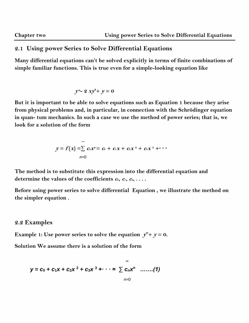
2.1 Using power Series to Solve Differential Equations
Many differential equations can’t be solved explicitly in terms of finite combinations of
simple familiar functions. This is true even for a simple-looking equation like
y n- 2 xy'+ y = 0
But it is important to be able to solve equations such as Equation 1 because they arise
from physical problems and, in particular, in connection with the Schrödinger equation
in quan- tum mechanics. In such a case we use the method of power series; that is, we
look for a solution of the form
y = f (x) =∑ cnxn = c0 + c1x + c2x 2 + c3x 3 +· · ·
The method is to substitute this expression into the differential equation and
determine the values of the coefficients c0, c1, c2, . . . .
Before using power series to solve differential Equation , we illustrate the method on
the simpler equation .
2.2 Examples
Example 1: Use power series to solve the equation y”+ y = 0.
Solution We assume there is a solution of the form
y = c0 + c1x + c2x 2 + c3x 3 +· · · = ∑ cnxn …….(1)
∞
n=0
∞
n=0

Chapter two Using power Series to Solve Differential Equations
We can differentiate power series term by term, so
y' = c1 + 2c2x + 3c3x 2 +· · · = ∑ncnxn—1
n=1
y” = 2c2 + 2 · 3c3x + . . . = ∑ n(n — 1)cn xn—2 ………(2) n=2
In order to compare the expressions for y and y” more easily, we rewrite y” as follows
4- y” =∑(n + 2)(n + 1)cn +2xn
Substituting the expressions in Equations 2 and 4 into the differential equation, we obtain
∑ (n + 2)(n + 1)cn+2xn +∑cn xn = 0
or
∑ [(n + 2)(n + 1)cn+2 + cn] xn = 0 ………(3)
If two power series are equal, then the corresponding coefficients must be equal. There- fore, the coefficients of xn in Equation 5 must be 0:
(n + 2)(n + 1)cn+2 + cn = 0
CN+2= - 𝑪𝒏
(𝒏 + 𝟏)(𝒏 + 𝟐) n=0,1,2,3, …. (4)
∞
∞
n=2
∞
n=0
∞
n=0 n=0
n=0
Chapter two Using power Series to Solve Differential Equations
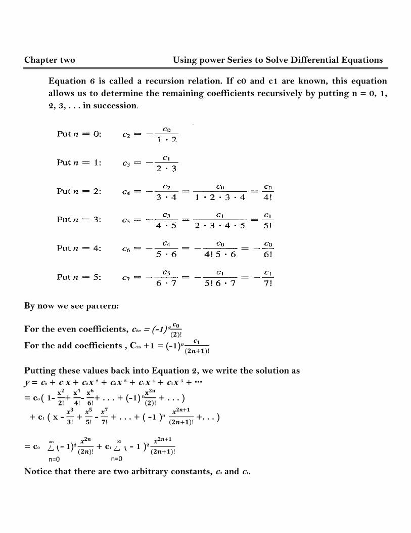
Equation 6 is called a recursion relation. If c0 and c1 are known, this equation
allows us to determine the remaining coefficients recursively by putting n = 0, 1,
2, 3, . . . in succession.
By now we see pattern:
For the even coefficients, c2n = (-1) 2𝒄𝟎
(𝟐)!
For the add coefficients , C2n +1 = (-1)n 𝒄𝟏
(𝟐𝒏+𝟏)!
Putting these values back into Equation 2, we write the solution as
y = c0 + c1x + c2x 2 + c3x 3 + c4x 4 + c5x 5 + ···
= c0 ( 1- 𝐱𝟐
𝟐!+
𝐱𝟒
𝟒!-
𝐱𝟔
𝟔!+ . . . + (-1) n
𝐱𝟐𝐧
(𝟐)! + . . . )
+ c1 ( x - 𝒙𝟑
𝟑! +
𝒙𝟓
𝟓! -
𝒙𝟕
𝟕! + . . . + ( -1 )n
𝒙𝟐𝒏+𝟏
(𝟐𝒏+𝟏)! +. . . )
= c0 ∑ (- 1)2 𝒙𝟐𝒏
(𝟐𝒏)! + c1 ∑ ( - 1 )2
𝒙𝟐𝒏+𝟏
(𝟐𝒏+𝟏)!
Notice that there are two arbitrary constants, c0 and c1.
n=0
∞
n=0
∞
Chapter two Using power Series to Solve Differential Equations
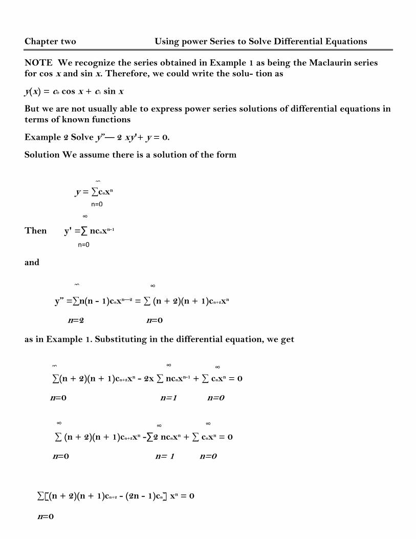
NOTE We recognize the series obtained in Example 1 as being the Maclaurin series for cos x and sin x. Therefore, we could write the solu- tion as
y(x) = c0 cos x + c1 sin x
But we are not usually able to express power series solutions of differential equations in terms of known functions
Example 2 Solve y”— 2 xy'+ y = 0.
Solution We assume there is a solution of the form
y = ∑cnxn
Then y' =∑ ncnxn-1
and
y” =∑n(n - 1)cnxn—2 = ∑ (n + 2)(n + 1)cn+2xn
n=2 n=0
as in Example 1. Substituting in the differential equation, we get
∑(n + 2)(n + 1)cn+2xn - 2x ∑ ncnxn-1 + ∑ cnxn = 0
n=0 n=1 n=0
∑ (n + 2)(n + 1)cn+2xn -∑2 ncnxn + ∑ cnxn = 0
n=0 n= 1 n=0
∑[(n + 2)(n + 1)cn+2 - (2n - 1)cn] xn = 0
n=0
∞
n=0
∞
n=0
∞ ∞
∞ ∞ ∞
∞ ∞ ∞

Chapter two Using power Series to Solve Differential Equations
This equation is true if the coefficient of xn is 0:
(n + 2)(n + 1)cn+2 - (2n - 1)cn = 0
cn+2 = 𝟐𝒏− 𝟏
(𝒏 + 𝟏)(𝒏 + 𝟐) cn n = 0, 1, 2, 3, …
We solve this recursion relation by putting n = 0, 1, 2, 3, . . . successively in Equation :
cn+2 = 𝟐𝒏− 𝟏
(𝒏 + 𝟏)(𝒏 + 𝟐) cn n = 0, 1, 2, 3, …
Put n = 0: C2= −𝟏
𝟏.𝟐 C0
Put n = 1: C3 = 𝟏
𝟐.𝟑 C1
Put n = 2: C4 = 𝟑
𝟑.𝟒 C2 = -
𝟑
𝟏.𝟐.𝟑.𝟒 C0 =
𝟑
𝟒! C0
Put n = 3: C5 = 𝟓
𝟒.𝟓 C3 =
𝟏.𝟓
𝟐.𝟑.𝟒.𝟓 C1 =
𝟏.𝟓
𝟓! C1
Put n = 4: C6 = 𝟕
𝟓.𝟔 C4 = -
𝟑.𝟕
𝟒!𝟓.𝟔 C0 = -
𝟑.𝟕
𝟔! C0
Put n = 5: C7 = - 𝟗
𝟔.𝟕 𝑪𝟓 =
𝟏.𝟓.𝟗
𝟓!𝟔.𝟕 𝑪𝟏 = -
𝟏.𝟓.𝟗
𝟕! C1
Put n = 6: C8 = 𝟏𝟏
𝟕.𝟖C6 = -
𝟑.𝟕.𝟏𝟏
𝟖! C0
Put n = 7: C9 = 𝟏𝟑
𝟖.𝟗 C7 =
𝟏.𝟓.𝟗.𝟏𝟑
𝟗! C1
In general, the even coefficients are given by
C2n = - 𝟑.𝟕.𝟏𝟏…..(𝟒𝒏−𝟓)
(𝟐𝒏)! C0
and the odd coefficients are given by
C2n+1= 𝟏.𝟓.𝟗…..( 𝟒𝒏−𝟑 )
(𝟐𝒏+𝟏)! C1

Chapter two Using power Series to Solve Differential Equations
The solution is
y= C0 + C1 X + C2 X2 + C3 X3 + C4 X4 + . . .
= C0 ( 1 - 𝟏
𝟐! X2 -
𝟑
𝟒! X4 -
𝟑.𝟕
𝟔! X6 -
𝟑.𝟕.𝟏𝟏
𝟖! X8 - . . . )
+ C1 ( X + 𝟏
𝟑! X3 +
𝟏.𝟓
𝟑! X5 +
𝟏.𝟓.𝟗
𝟕! X7 +
𝟏.𝟓.𝟗.𝟏𝟑
𝟗! X9 + . . . )
Or
y = C0 ( 1 - 𝟏
𝟐! X2 - X2n )
+ C1 ( X + X2n+1 )
Note : In Example 2 we had to assume that the differential equation had a series
solution . But now we could verify directly that the function given by Equation 8 is
indeed a solution .
Note : Unlike the situation of Example 1 , the power series that arise in the solution of
Example 2 do not define elementary functions . The functions .
y1 ( X ) = 1 - 𝟏
𝟐! X2 - X2n
and
y2 ( X) = X + X2n+1
are perfectly good functions but they can’t be expressed in terms of familiar functions.
We can use these power series expressions for y1 and y2 to compute approximate values
of the functions and even to graph them. Figure 1 shows the first few partial sums T0
,T2 , T4 , . . .(Taylor polynomials) for y1 ( X ) , and we see how they converge to y1 . In
this way we can graph both and in Figure 2.
∑3.7. . . . (4n − 5)
(2n)!
∞
𝑛=2
∑1 .5 .9 . . . . . (4𝑛 − 3 )
(2𝑛 + 1)!
∞
𝑛=1
∑3 .7 . . . . . . (4𝑛 − 5 )
(2𝑛)!
∞
𝒏=𝟐
∑1 .5 .9 . . . . . (4𝑛 − 3 )
(2𝑛 + 1)!
∞
𝑛=1

Chapter two Using power Series to Solve Differential Equations
NOTE : If we were asked to solve the initial-value problem .
y" – 2xy' + y = 0 y (0) = 0 y' (0) = 1
We would observe that
C0 = y (0) = 0 C1 = y' (0) = 1
This would simplify the calculations in Example 2, since all of the even coefficients
would be 0. The solution to the initial-value problem is :
y (X) = X + X2n+1
∑1 .5 .9 . . . . . (4𝑛 − 3 )
(2𝑛 + 1)!
∞
𝑛=1

References
[1] K.M. Mohammed ,"On Solution of Two Point Second Order
Boundary Value Problems by Using Semi-Analytic Method", MSc
thesis, University of Baghdad, College of Education – Ibn – Al-
Haitham, 2009 .
[2] K. S. Mc Fall, "An Artificial Neural Network Method for Solving
Boundary Value Problems with Arbitrary Irregular Boundaries ",
PhD Thesis , Georgia Institute of Technology , 2006 .
[3] K. S. Mc Fall and J. R. Mahan, " Investigation of Weight Reuse
in Multi-Layer Perceptron Networks for Accelerating the Solution
of Differential Equations ",IEEE International Conference on
Neural Networks, Vol.14, pp:109-114, 2004.
[4] L.N.M.Tawfiq and Q.H.Eqhaar, "On Multilayer Neural
Networks and its Application For Approximation Problem ", 3rd
scientific conference of the College of Science ", University of
Baghdad. 24 to 26 March 2009.
[5] L.N.M.Tawfiq and Q.H.Eqhaar, "On Radial Basis Function
Neural Networks, Al-Qadisiyah Journal for Pure Sciences", Vol. 12
, No. 4, 2007