Zachi Baharav

000064130

May-05-2009

Course: Methods 394.

Prof. Cheryl Roddick.

Unit Plan: Differential equations

This document includes the following items:

1. 1-page summary of the unit plan.

2. Items mandated by the format of this assignment.

3. General considerations in the design of the unit.

4. Short description of lesson plans + Elaboration on 2 lessons.

5. Assessment.

Appendix A: Calendar.

Appendix B: Calculus AB and BC requirements.

Appendix C: Unit Summary work-sheet.

In addition, accompanying this document are PowerPoint slides on the rubric and assessment, and the unit-test

assessment itself.

1. Unit Plan: Differential Equations

Lesson #

Subject Details Special comments / HW*

1 * Introduction. *Connection to Prior-knowledge. * Motivation. * Map of the unit + description. * Terms we will use. * Verifying solution.

2 * General solution and verifying solution. * Initial conditions and Particular solution.

* Use simple cases students already know how to solve. * Important: The solution is a FUNCTION, not a number!

3 *Word problem. * Putnam question.

* Simple worddrawingEquation. * Introduce Putnam exams. Introduce the problem at hand.

“Problem-Solving”

4 * Solution curves + Slope fields.

* Start plotting on transparencies.

5 * Unit project intro. * Reading on application.

* This can be moved around. * Reading: Soccer-Ball, Navier-Stokes.

“Literacy-Friday” Collect Class Journals

6 * Slope fields (cont.) * This is one of the critical subjects, so worth spending another full lesson on!

Start introducing some AP question every day.

7 * Separation of Variables.

* The only method tested.

8 * Exponential solutions.

* Exponential solutions – Most important

ones!

9 *Problem solving: word problem.

* Understanding the concept of one-value + differential eqn get any value.

“Problem-Solving”

10 * Unit project. * Finishing it all up. * Write three question (+solutions) for the test: Easy, Medium, Hard.

“Literacy-Friday” Collect Class Journals

11 * Match the cards game * This is a good review game, that combines a lot of the previous concepts.

“Problem-Solving”

12 *Presentation of unit-projects.

* Peers evaluation.

13 *Unit-Review. * Summary sheet.

14 *Test.

* Homework practice – didn’t include these ones here.

Some things I changed from my previous plan: 1. Took off Euler method (1-lesson). 2. Explicitly put in ‘Literacy Friday’ and ‘Problem Solving’. 3. Removed some of the ‘Working in class on Unit Project’.

Questions: zachi@baharav.org Online info: www.baharav.org

2. Items mandated for the format of this assignment.

2.1 Unit Title – Differential Equations

2.2 Course – Calculus AB

2.3 Time allotted – 15 days (Including Test, test-return, and so on).

2.4 Goals – The students will be able to create, manipulate, and interpret Differential Equations (at the

appropriate level).

2.5 Objectives – The above goal is first translated into the more practical goal of preparing students for the

AP test on this subject. Breaking it down to specific objectives, at the completion of this unit, the

students should:

2.5.1 Familiar with terms relating to differential equations. (Bloom’s (1) Remembering)

2.5.2 Be able to find general solution and particular solution. (Bloom’s (2) Understanding and (3)

Applying)

2.5.3 Can draw solution curves. (Bloom’s (2) Understanding and (3) Applying )

2.5.4 Can draw slope fields. (Bloom’s (2) Understanding)

2.5.5 Can relate slope-fields to solution curves. (Bloom’s (2) Understanding and (3) Applying, and

also (5) Synthesis – putting things together)

2.5.6 Can solve word problems using differential equations. (It starts with the lower levels, but

climbs to (4) Analysis and (5) Synthesis - See for example the Putnam problem).

2.5.7 Can verify and interpret a solution. (Bloom’s (6) Evaluation).

2.6 NCTM Standards – As mentioned above, this course is driven more by the requirements of the College

Board AP- test requirements, which are given in Appendix A, but just to highlight the relevant part here:

“

Applications of derivatives (just pointing to the one relevant for this unit)…

Geometric interpretation of differential equations via slope fields and the relationship between slope fields and solution curves for differential equations

“

OF course, this unit addresses some of the ideas in the NCTM Standards, but it ventures to do it in a

subject-matter beyond the scope the NCTM covers (High-School). The items of the NCTM which are

addressed here are Problem-Solving, Connections, and Representation. This is especially true as this unit

combines many of the ideas learned in calculus into applicable Physics problems. This is the point to

mention that many of the students also take Physics AP, and therefore many of the problems will be

related to real-world physics problems.

2.7 California Standards – Amazingly enough, California Standards do venture into this area as well, even

though they do admit that one may take into consideration the College Board syllabi for Calculus AB as a

guide. The relevant item is:

“

27.0 Students know the techniques of solution of selected elementary differential equations and their

applications to a wide variety of situations, including growth-and-decay problems.

“

2.8 Prerequisite Knowledge and Skills – The students should master basic integration and differentiation

techniques. These are all part of the course syllabus before we reach this unit.

2.9 Lessons – See below.

2.10 Assessment – See below.

2.11 Resources:

2.11.1 Course Text-Book – “Calculus with Analytic Geometry”, 8th edition, by Larson, Hostetler, and

Edwards. Publisher: Houghton Mifflin Company. We cover most of Chapter 6: “Differential

Equations”

2.11.2 “Match the Card” Game – Houston Area Calculus Teachers Workshop Materials:

http://www.houstonact.org/HoustonACTmaterials.htm , and specifically there see :

http://www.houstonact.org/documents/StephensonSFCardMatch.pdf .

2.11.3 Literacy – Plus magazine: http://plus.maths.org/ , and also Nrich:

http://nrich.maths.org/public/ .

3. Considerations in the unit design. Top Down considerations: “External constraints”

1. About 2.5 weeks for the whole unit (not less than 2 weeks, and not more than 3 weeks).

2. Cover Chapter 6 in the book: “Differential Equations”. This covers material needed for the AP exam.

Bottom up considerations: Things we view as focal points to the subject.

NOTE: According to the curriculum required for the AP Calculus AB and BC: (See Appendix A)

AB: • Geometric interpretation of differential equations via slope fields and the relationship between slope fields and solution curves for differential equations

BC adds: + Numerical solution of differential equations using Euler’s method

Below is the material in the chapter, and I will comment on which I think is relevant in light of the above:

1. Introduction: Needed. This is plenty, and some is really important, and will take a few lessons to cover.

a. General solution.

b. Verifying solution

c. Characteristic curves.

d. Initial conditions and Particular solution.

2. Slope fields. Needed for AB!

3. Euler’s method – numerical approximation of solution. Somewhat confusing for students. Will cover in BC.

4. Separation of variables: Useful to go over just because they use it all the time.

a. Exponential solution: Growth and Decay. important example/application

i. Constant as a multiplier rather than addition.

ii. Make sure students realize that there are equivalent forms: 𝑒−𝑎𝑡 = 𝑒−𝑎 𝑡 .

b. Logistic equation. Possibly important example/application, but not as much as exponentials.

c. Good application to explore: Finding orthogonal trajectories.

5. Homogeneous equation. Skip

6. First order linear differential equation. Skip

7. Bernoulli equation. Skip

Lateral considerations: A project to span the whole unit.

We will have a unit-project that will span the whole unit period. Will start in the first week, and will be finished and

presented by the end of the unit. It will be done in groups. Description of the project is in a separate document.

Also, including “Literacy-Friday” and “Problem-solving” Wednesday.

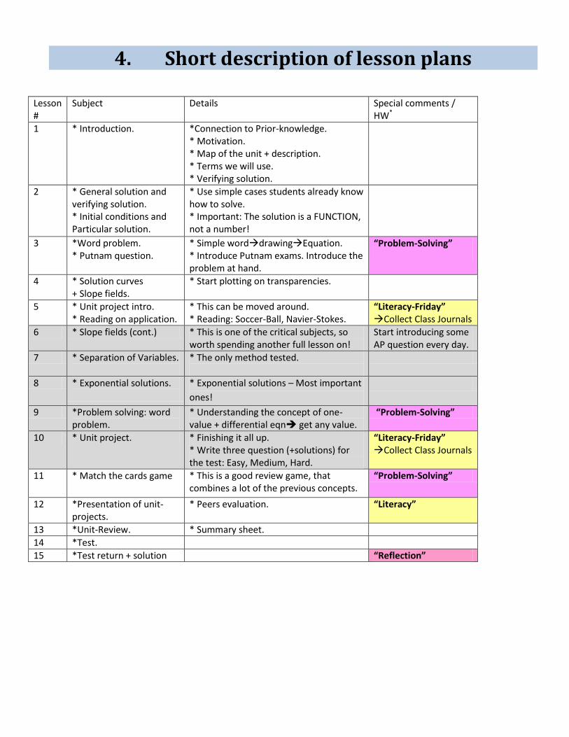
4. Short description of lesson plans

Lesson #

Subject Details Special comments / HW*

1 * Introduction. *Connection to Prior-knowledge. * Motivation. * Map of the unit + description. * Terms we will use. * Verifying solution.

2 * General solution and verifying solution. * Initial conditions and Particular solution.

* Use simple cases students already know how to solve. * Important: The solution is a FUNCTION, not a number!

3 *Word problem. * Putnam question.

* Simple worddrawingEquation. * Introduce Putnam exams. Introduce the problem at hand.

“Problem-Solving”

4 * Solution curves + Slope fields.

* Start plotting on transparencies.

5 * Unit project intro. * Reading on application.

* This can be moved around. * Reading: Soccer-Ball, Navier-Stokes.

“Literacy-Friday” Collect Class Journals

6 * Slope fields (cont.) * This is one of the critical subjects, so worth spending another full lesson on!

Start introducing some AP question every day.

7 * Separation of Variables.

* The only method tested.

8 * Exponential solutions.

* Exponential solutions – Most important

ones!

9 *Problem solving: word problem.

* Understanding the concept of one-value + differential eqn get any value.

“Problem-Solving”

10 * Unit project. * Finishing it all up. * Write three question (+solutions) for the test: Easy, Medium, Hard.

“Literacy-Friday” Collect Class Journals

11 * Match the cards game * This is a good review game, that combines a lot of the previous concepts.

“Problem-Solving”

12 *Presentation of unit-projects.

* Peers evaluation. “Literacy”

13 *Unit-Review. * Summary sheet.

14 *Test.

15 *Test return + solution “Reflection”

(If you wish to see full lesson plans on these subjects, you can find most on www.baharav.org/math . Here, however, I changed order and added more literacy/problem-solving in an explicit manner. So the regular plans are all there, but might be in different order).

Lesson-1 - Introduction. Learning Objectives:

o Place of unit in the scheme of things taught in this semester. o Motivation for the subject. o Description of the unit content. o First intro of unit project. o Some terms we will use.

Lesson-2 – General solution and Particular solution – The students already encountered the integration constant previously in the course. This lesson is therefore more of placing this all in the new context, and familiarity with the terms and their meaning (e.g., initial condition). Learning Objectives

o Recognize multiplicity of general solution. o Using initial condition, reducing it to particular solution.

Lesson 3 – “Problem Solving Wednesday” – word problem and Putnam question. o Introduce the Putnam competition (What it is, history, etc).

o Go over the question, explain how to attack it, then dissect it, explain terms, and finally emphasize the

notion that the differential equation describes the SLOPE of the tangent to the solution curve in a point.

Do not completely solve: Give them the chance to do it.

o Emphasize the need for ‘problem solving’ skills.

Question:

Prove that if the family of integral curves of the differential equation

𝑑𝑦

𝑑𝑥+ 𝑃 𝑥 ∗ 𝑦 = 𝑞 𝑥 , 𝑝 𝑥 ∗ 𝑞 𝑥 ≠ 0

is cut by the line x=k, the tangents at the points of intersection are concurrent.

Lesson 4 – Solution curves + Slope Fields – Keep in mind the students already saw slope-fields earlier in the book. We can just review what it is, and the main thing here is to show the connection to the solution curves. Learning Objectives

o Given general solution, draw solution curves. o Two ways to get to slope-fields:

From the derivatives of the solution curves. From the differential equation.

o See the various relations between Solution-curves and Slope-field. (Use transparencies to show the relation!)

Lesson 5 – Literacy Friday – Introduce Unit project, and reading on application. See full lesson plan below. Learning Objectives

o What is the unit-project. o Students will know their group, project subject, expectations from a complete project, and the time line. o Reading a piece on the application of Differential Equations to Soccer:

http://plus.maths.org/latestnews/may-aug06/teamgeist/index.html

Lesson 6 – Slope fields – extra exercise. See full lesson plan below. Practice and apply the various aspects of Slope-fields in a social setting (Speed-dating mode, in order to cover a lot of stuff).

Lesson 7 – Separation of Variables – The students already use it and are familiar with this. Learning Objectives

o Formally introduce the method of Separation of Variables.

Lesson 8 – Exponential Solutions – This is probably the most important and widely encountered solution, and specifically highlighted in the California standards. Learning Objectives

o An application to exponential curves solutions. o Half-life time, and behaviors as t grows, or at t=0.

Lesson 9 – Problem solving – We will dwell over the following two questions. One is a word-problem, and the other requires understanding of the concept of derivative of a question.

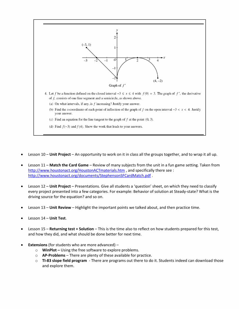
Lesson 10 – Unit Project – An opportunity to work on it in class all the groups together, and to wrap it all up.

Lesson 11 – Match the Card Game – Review of many subjects from the unit in a fun game setting. Taken from http://www.houstonact.org/HoustonACTmaterials.htm , and specifically there see : http://www.houstonact.org/documents/StephensonSFCardMatch.pdf .

Lesson 12 – Unit Project – Presentations. Give all students a ‘question’ sheet, on which they need to classify every project presented into a few categories. For example: Behavior of solution at Steady-state? What is the driving source for the equation? and so on.

Lesson 13 – Unit Review – Highlight the important points we talked about, and then practice time.

Lesson 14 – Unit Test.

Lesson 15 – Returning test + Solution – This is the time also to reflect on how students prepared for this test, and how they did, and what should be done better for next time.

Extensions (for students who are more advanced) – o WinPlot – Using the free software to explore problems. o AP-Problems – There are plenty of these available for practice. o TI-83 slope field program - There are programs out there to do it. Students indeed can download those

and explore them.

Differential Equations: Calculus AB Lesson Plan 5: Unit Project + Literacy Friday

Overview

This serves to set up the Unit-project. The students will work on it as groups, and present it at the end of the unit.

In the second half we will read a text describing an application.

Learning Objectives

What is the unit-project.

Students will know their group, project subject, expectations from a complete project, and the time line.

Read on real-world application.

Prior Knowledge needed

The students are already in the unit, so they will know ‘some’ of the project elements. Depending on when it is

presented exactly during the unit, they might know more (or less).

Materials

Handout of unit-project.

Handout of the article we will read. See copies below!

Instruction and activity

1. Unit project:

a. It’s place in the unit as tying all subjects touched.

b. Component of grade.

c. Will be done in groups during a few lessons, and

eventually presentation.

d. We will be filling things in it as we learn them.

2. Go over the handout.

3. Go over a sample project. <- I have one in transparencies that I shared (Because they also made it on

transparencies)!

a. Show ‘fact gathering’ phase.

b. Final result.

4. Getting ready with groups, and maybe start working on it (time permitting).

5. Reading article:

a. Describe (show) the two ball designs:

zachi@baharav.org www.baharav.org

Use of cooperative learning activity:

Different people in the group took

responsibility for different parts, and later

on combined it all together. For example:

doing the slope fields, drawing solutions,

history part, application, and so forth.

Bloom’s Taxonomy used here:

From (3) Application (solving the problem), to

(5) Synthesis – putting equations and graphs

together, to (6) Evaluation – evaluating peers

projects for correctness and fit into the

worksheet I hand out at the end.

The (4) Analysis also comes into play in the

project when students look for application:

Students need to be able to go from the real-

world application into the equation.

• Pre-reading: Anticipation questions:

– Do you think there will be any difference in behavior between old-ball and new-ball?

• If yes, What?

• If no, Why?

– What may cause a change of behavior in a new ball design?

• Short discussion, followed by silent reading.

• Full class discussion of the result, and then a video from youTube on the two balls.

6. Home Practrice:.

7. Wrap-up : A big project, with many parts, which we will work on during a few sessions. We’ll monitor progress

as we go.

====End====

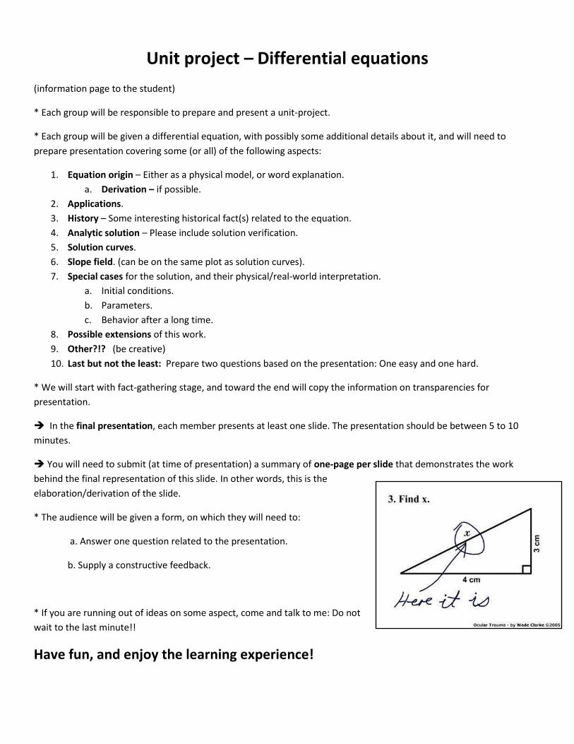
Unit project – Differential equations

(information page to the student)

* Each group will be responsible to prepare and present a unit-project.

* Each group will be given a differential equation, with possibly some additional details about it, and will need to

prepare presentation covering some (or all) of the following aspects:

1. Equation origin – Either as a physical model, or word explanation.

a. Derivation – if possible.

2. Applications.

3. History – Some interesting historical fact(s) related to the equation.

4. Analytic solution – Please include solution verification.

5. Solution curves.

6. Slope field. (can be on the same plot as solution curves).

7. Special cases for the solution, and their physical/real-world interpretation.

a. Initial conditions.

b. Parameters.

c. Behavior after a long time.

8. Possible extensions of this work.

9. Other?!? (be creative)

10. Last but not the least: Prepare two questions based on the presentation: One easy and one hard.

* We will start with fact-gathering stage, and toward the end will copy the information on transparencies for

presentation.

In the final presentation, each member presents at least one slide. The presentation should be between 5 to 10

minutes.

You will need to submit (at time of presentation) a summary of one-page per slide that demonstrates the work

behind the final representation of this slide. In other words, this is the

elaboration/derivation of the slide.

* The audience will be given a form, on which they will need to:

a. Answer one question related to the presentation.

b. Supply a constructive feedback.

* If you are running out of ideas on some aspect, come and talk to me: Do not

wait to the last minute!!

Have fun, and enjoy the learning experience!

Group 1: RC-Circuit with Voltage Source.

𝑅𝐶𝑑𝑉

𝑑𝑡+ 𝑉 = 𝑉𝑠 ; 𝑉(𝑡 = 0) = 0

V(t) is the unknown function. R (resistor), C (Capacitor) , and 𝑉𝑠 (Voltage source) are all known constants.

Group 2: RC-Circuit.

𝑅𝐶𝑑𝑉

𝑑𝑡+ 𝑉 = 0 ; 𝑉 𝑡 = 0 = 𝑉0

V(t) is the unknown function. R (resistor), C (Capacitor) , and 𝑉0 (Initial Voltage) are all known constants.

Group 3: RL-Circuit with Voltage Source.

𝐿𝑑𝐼

𝑑𝑡+ 𝑅𝐼 = 𝑉𝑠 ; 𝐼(𝑡 = 0) = 0

I(t) is the unknown function. R (resistor), L (Inductor) , and 𝑉𝑠 (Voltage source) are all known constants.

Group 4: RL-Circuit.

𝐿𝑑𝐼

𝑑𝑡+ 𝑅𝐼 = 0 ; 𝐼 𝑡 = 0 = 𝐼0

I(t) is the unknown function. R (resistor), L (Inductor) , and 𝐼0 (Initial current) are all known constants.

Group 5: Non linear RC Circuit. (Desoer and Kuh, pp. 116-117) (H)

(where 𝐼𝑅 = 𝑉𝑅3 , and assume C=1F)

𝐶𝑑𝑉

𝑑𝑡+ 𝑉3 = 0 ; 𝑉(𝑡 = 0) = 0

Group 6: Mass Moving on a Plane with Friction.

𝑀𝑑𝑣

𝑑𝑡= −𝐵𝑣 ; 𝑣(𝑡 = 0) = 𝑣0

M – known mass ; B – Known friction coefficient ; 𝑣(𝑡) – unknown function to be determined.

Group 7: Population Growth Models. (H)

𝑑𝑁

𝑑𝑡= 𝑘𝑁 𝑁𝑒𝑞𝑢𝑖 – 𝑁 ; 𝑁 𝑡 = 0 = 𝑁0

𝑁(𝑡) is the population number, to be solved for. 𝐾, 𝑁𝑒𝑞𝑢𝑖 , and 𝑁0 are known constants.

Group 8: Radioactive Decay.

𝑑𝑚

𝑑𝑡= −𝑘𝑚 ; 𝑚 𝑡 = 0 = 𝑚0

𝑚(𝑡) is the mass to be solved for. 𝑘 and 𝑚0 are known constants.

(In reality, we gave (they picked) also other equations from Biology etc…)

The Teamgeist has a distinctly

different construction than past footballs, with only 14 panels.

Eye on the ball

England will play Portugal in the World Cup quarterfinals on Saturday night, but it might come down to goalkeeper Paul Robinson versus

Teamgeist — the new World Cup ball.

The ball has drawn criticism from a number of goalkeepers for its unpredictable movement in the air. Robinson told BBCSport the ball was "very goalkeeper unfriendly" and that it moves "about

all over the place". And goalkeepers are not the only ones commenting on the Teamgeist's design: scientists agree that it could cause some upsets in this year's competition.

Teamgeist (which means team spirit in German) has a very unusual construction consisting of just 14 curved

panels wrapping around the football. This is a dramatic change from the 32 panel (12 pentagons and 20

hexagons) balls used in the World Cup since 1970.

Adidas, who created the Teamgeist for the World Cup, say their design gives the ball an almost

perfectly spherical shape and makes it the most accurate ball ever. But scientists claim that in certain instances, this smoother shape could make

the ball wildly unpredictable in flight because of the aerodynamics of its design.

Dr. Ken Bray, a sports scientist at the University

of Bath, studies the aerodynamics of footballs in flight. The movement of a ball through the air can be described by differential equations, one equation

for each of the three dimensions. The basis for this description are the Navier-Stokes equations, which describe

the behaviour of any fluid, and are used in many applications such as weather prediction.(You can read more about the Navier-Stokes equations in How maths can make you rich and

famous from issue 25 of Plus, and about weather prediction inAnd now, the weather....)

These complicated equations cannot be easily solved, but Bray can find approximate solutions which explain the behaviour of a ball in flight. And the findings from Bray's research indicate there may be a mathematical truth behind Robinson's concerns about the Teamgeist — the ball

is not aerodynamically stable.

When a ball is kicked slowly, the airflow separates from the ball leaving a large zone of turbulence behind it, creating drag which slows the ball down. But over a certain speed, 12mph

for a football, the airflow sticks to the surface of the ball for longer, and this late separation results in less turbulence and reduced drag. This thin layer of airflow clinging very close to the surface of the ball is called the boundary layer. When the boundary layer is created, or "tripped",

the ball will move in a much more predictable way. (You can read more detail about tripping the boundary layer in Bray's article The science behind the swerve on the BBC.)

It is now understood that surface imperfections, such as the seams on a football, contribute to

the boundary layer being tripped: more imperfections result in improved aerodynamic stability.

However the Teamgeist's 14 panels gives it less seams than other footballs, and this is the factor that makes Bray fear for Robinson and his goalkeeping peers.

It appears that the boundary layer is tripped by discontinuities being present on particular

sections of the ball as it moves during its flight. This is not a problem if the ball is spinning quickly enough — the quick rotation means that, on average, a seam will be where needed to

trip the boundary layer more or less continuously.

"Because the Teamgeist ball has just 14 panels it is aerodynamically more similar to the baseball which only has two panels," Bray says. And what goalkeepers have to watch out for is the equivalent of baseball's knuckleball — when the ball has very little spin at all. Due to the fewer

seams on the Teamgeist, they may move in and out of the right location to trip the boundary layer, so the ball will veer between stable and unstable movement in the air.

"Occasionally pitchers will throw a 'knuckleball' which bobs about randomly in flight and is very

disconcerting for batters. It happens because pitchers throw the ball with very little spin and as the ball rotates lazily in the air, the seam disrupts the air flow around the ball at certain points

on the surface, causing an unpredictable deflection."

So if we're lucky (and Robinson or one of his peers isn't), we might see the first of a new breed of goal — the knucklegoal. "Watch the slow motion replays to spot the rare occasions where the ball produces little or no rotations," says Bray, "and where goalkeepers will frantically attempt to

keep up with the ball's chaotic flight path."

But 14 panels or 32, with the best players from around the world in Germany this summer, we can look forward to many spectacular saves — as well as many spectacular goals.

Navier-Stokes equations fluid mechanicsmathematics in

sport football statistics aerodynamicsdifferential equation turbulence mathematical modellingprobability Rachel Thomas

Differential Equations: Calculus AB Lesson Plan 6: Slope fields.

Overview

After learning about Slope fields, and their relation to other aspects of the differential equation, we will get our feet wet

with plenty of examples.

Learning Objectives

Practice the various aspects of Slope Fields.

Prior Knowledge needed

The students should have learned in the previous lesson slope-fields

and solution-curves, and the relation therein.

Special Materials

Work sheet: See below (one page, double sided).

Transparencies + Sharpies for students to draw their group work.

Instruction and activity

1. Warm-up problem (from AP), and by that review of what we did yesterday.

2. Group work w/presentations:

The idea is to let the student solve, and see, quite a few slope-field equations, while not getting bored. Various

options:

a. Speed dating mode very useful to covering a lot of stuff quickly, and with different partners.

Or alternitvally:

b. Small groups, and then switch.

At any rate, at the end (last session), need to draw on Transparencies so we can all share.

The students will solve the following question, for each:

a. Draw slope field.

b. Draw solution curves (if needed and possible, solve equation first).

c. Draw a particular solution using the initial conditions.

The 4 questions will be on the sheet handed out. See at the bottom.

3. Presentation of the solution and discussions.

a. Teacher can use Winplot to share results of slope-fields and equations.

4. Wrap-up : Two options.

zachi@baharav.org www.baharav.org

Use of cooperative learning activity: In

many groups the kids parted into doing

the slope-field and the general solution,

and then checked each other and

combined results.

a. We mentioned a few concepts. Write down what the connection between those is:

i. Differential equation

ii. Solution curves

iii. Slope curve

iv. Particular solution

OR

b. Which was the hardest one for you to solve (question and item) ? Why? Which was the easiest?

5. Home Practice assignments.

====End==== (Well, the worksheet is below)

Student Name: ____________________________________ Date:__________________

Slope Field worksheet

NOTE: NOT every tick on the grid should be taken as ‘1’, and slope fields should NOT be drawn on each point. Use your own

judgment for how to do it.

𝑑𝑦

𝑑𝑥 = 𝑐𝑜𝑠(𝑥) ; y(0)=1

* Draw slope field.

* Draw solution curves (solve equation first).

* Draw a particular solution using the initial conditions.

𝑑𝑦

𝑑𝑥 = 3𝑥2 − 4 ; y(0)=-1

* Draw slope field.

* Draw solution curves (solve equation first).

* Draw a particular solution using the initial conditions.

Bloom’s (3) Application

Bloom’s (3) Application

AND (5) Synthesis –

Looking for a fit between

the slope field and

solutions, and Particular

solution.

𝑑𝑦

𝑑𝑥 = 𝑥 + 𝑦 ; y(0)=1

* Draw slope field.

* Draw solution curves.

Check the possible solution: 𝑦 = 𝑘𝑒𝑥 − 1 − 𝑥 .

What’s special about this solution?!?

* Draw a particular solution using the initial conditions.

𝑑𝑦𝑑𝑥

=2𝑥

𝑦 ; y(1) = 1

* Draw slope field.

* Draw solution curves (solve equation first).

* Draw a particular solution using the initial conditions.

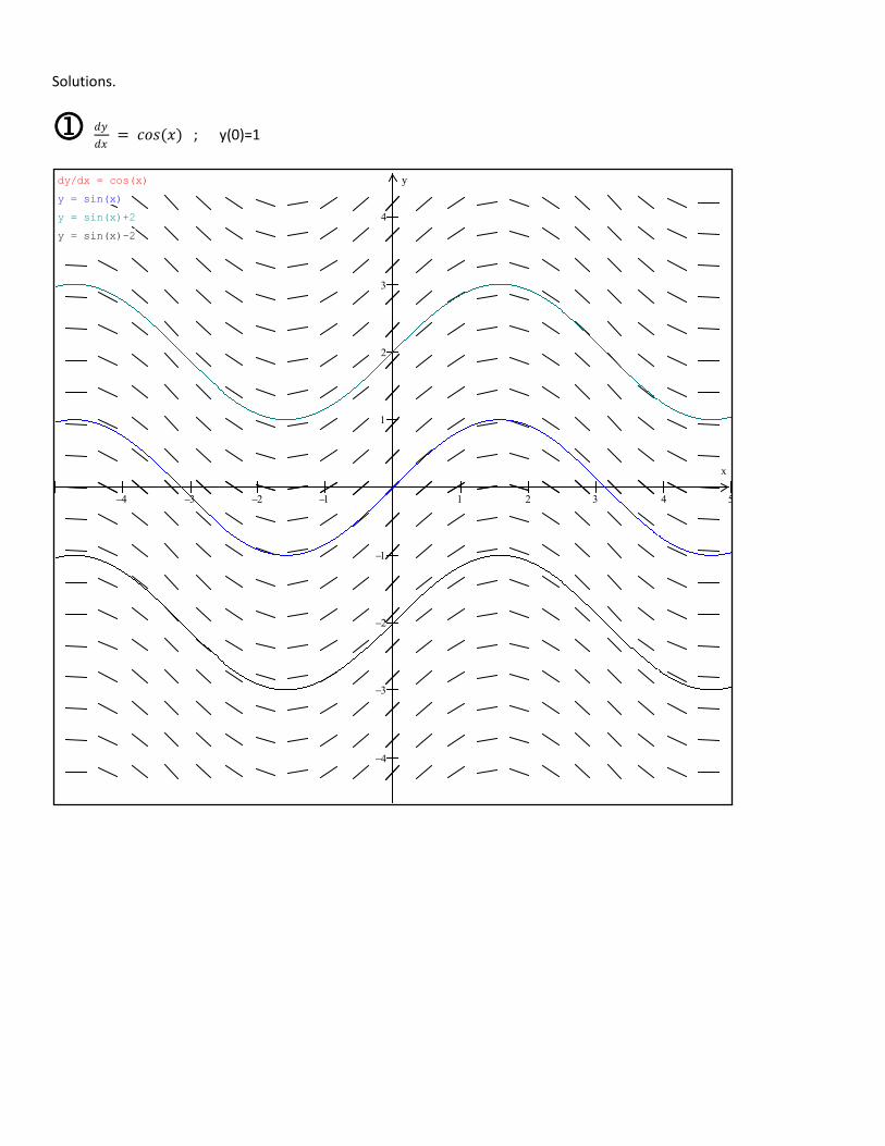
Solutions.

𝑑𝑦

𝑑𝑥 = 𝑐𝑜𝑠(𝑥) ; y(0)=1

x

ydy/dx = cos(x)

y = sin(x)

y = sin(x)+2

y = sin(x)-2

𝑑𝑦

𝑑𝑥 = 3𝑥2 − 4 ; y(0)=-1

x

ydy/dx = 3x^2-4

y = x^3-4x

y = x^3-4x-2

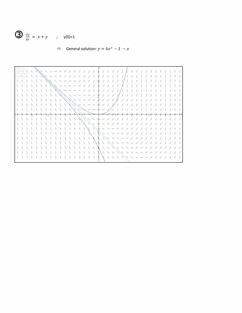
𝑑𝑦

𝑑𝑥 = 𝑥 + 𝑦 ; y(0)=1

General solution: 𝑦 = 𝑘𝑒𝑥 − 1 − 𝑥

x

ydy/dx = x+y

y = e^x-1-x

y = 0*e^x-1-x

y = -e^x-1-x

𝑑𝑦𝑑𝑥

=2𝑥

𝑦 ; y(1) = 1

==END (Of lesson plan on Slope Fields)===

x

ydy/dx = 2x/y

y = sqrt(2*x^2)

5. Assessment

See attached Power point for the rubric, and demonstration of its application to the unit test of a student. Other than the summative final unit-test, which is attached and is analyzed with its rubric in the slides, other means of assessments can be used throughout: 1. Homework practice assignments – The students get problems from the book, and submit those. 2. Group project – With a final presentation, it is an appropriate tool for assessment. See in the lesson plan

(Lesson 5) for the specifics details on Bloom’s taxonomy. 3. Group-work in class – For example, the problems solved in lesson-6 is a good chance to wander among the

groups and see how students are dealing with the subject matter. 4. AP-Problems – Every day, when solving an AP-Problem as a warm up, bringing up a student to the board is

another good way to evaluate. 5. Last but not the least: Extra-credit quizzes – For example, turning an AP-problem warm-up into an extra-

credit quiz is a good tool to evaluate where the class stands. As mentioned, the Bloom’s taxonomy specifics as applied to the assessment tools are described in the Project lesson plan and in the slides for the test.

Appendix A: Calendar Fe

bru

ary

2

00

9

Mon Tue Wed Thu Fri Sat Sun 1

2 3 4 5 6 7 8

9 10 11 12 13 14 15

16

Week off

17

In IHS

18

19

20

21 22

23 24 25 26 27 28

Mar

ch

20

09

Mon Tue Wed Thu Fri Sat Sun 1

2 3 4 5 6 7 8

9 10 11 12 13 14 15

16 17 18 19 20 21 22

23 24 25 26 27 28 29

30 31

Appendix B : Calculus AB and BC requirements.

Curriculum needed for the AP exam (and some details about the exams): Taken verbatim from : ap08_calculus_coursedesc.pdf :: http://www.collegeboard.com/student/testing/ap/calculus_ab/samp.html

===== Start of “Verbatim” from AP document===

Topic Outline for Calculus AB This topic outline is intended to indicate the scope of the course, but it is not necessarily the order in which the topics need to be taught. Teachers may fi nd that topics are best taught in different orders. (See AP Central [apcentral.collegeboard. com] for sample syllabi.) Although the exam is based on the topics listed here, teachers may wish to enrich their courses with additional topics. II. Derivatives Concept of the derivative • Derivative presented graphically, numerically, and analytically • Derivative interpreted as an instantaneous rate of change • Derivative defined as the limit of the difference quotient • Relationship between differentiability and continuity Derivative at a point • Slope of a curve at a point. Examples are emphasized, including points at which there are vertical tangents and points at which there are no tangents. • Tangent line to a curve at a point and local linear approximation • Instantaneous rate of change as the limit of average rate of change • Approximate rate of change from graphs and tables of values Derivative as a function • Corresponding characteristics of graphs of ƒ and ƒ_ • Relationship between the increasing and decreasing behavior of ƒ and the sign of ƒ_ • The Mean Value Theorem and its geometric interpretation • Equations involving derivatives. Verbal descriptions are translated into equations involving derivatives and vice versa. Second derivatives • Corresponding characteristics of the graphs of ƒ, ƒ_, and ƒ _ • Relationship between the concavity of ƒ and the sign of ƒ _ • Points of inflection as places where concavity changes Applications of derivatives • Analysis of curves, including the notions of monotonicity and concavity • Optimization, both absolute (global) and relative (local) extrema • Modeling rates of change, including related rates problems • Use of implicit differentiation to find the derivative of an inverse function • Interpretation of the derivative as a rate of change in varied applied contexts, including velocity, speed, and acceleration • Geometric interpretation of differential equations via slope fields and the relationship between slope fields and solution curves for differential equations

Computation of derivatives • Knowledge of derivatives of basic functions, including power, exponential, logarithmic, trigonometric, and inverse trigonometric functions • Derivative rules for sums, products, and quotients of functions • Chain rule and implicit differentiation

=====

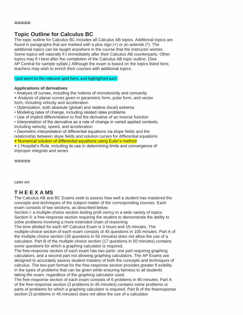
Topic Outline for Calculus BC The topic outline for Calculus BC includes all Calculus AB topics. Additional topics are found in paragraphs that are marked with a plus sign (+) or an asterisk (*). The additional topics can be taught anywhere in the course that the instructor wishes. Some topics will naturally fi t immediately after their Calculus AB counterparts. Other topics may fi t best after the completion of the Calculus AB topic outline. (See AP Central for sample syllabi.) Although the exam is based on the topics listed here, teachers may wish to enrich their courses with additional topics.

I just went to the relevant spot here, and highlighted part:

Applications of derivatives • Analysis of curves, including the notions of monotonicity and concavity + Analysis of planar curves given in parametric form, polar form, and vector form, including velocity and acceleration • Optimization, both absolute (global) and relative (local) extrema • Modeling rates of change, including related rates problems • Use of implicit differentiation to find the derivative of an inverse function • Interpretation of the derivative as a rate of change in varied applied contexts, including velocity, speed, and acceleration • Geometric interpretation of differential equations via slope fields and the relationship between slope fields and solution curves for differential equations + Numerical solution of differential equations using Euler’s method + L’Hospital’s Rule, including its use in determining limits and convergence of improper integrals and series

=====

Later on:

T H E E X A MS The Calculus AB and BC Exams seek to assess how well a student has mastered the concepts and techniques of the subject matter of the corresponding courses. Each exam consists of two sections, as described below. Section I: a multiple-choice section testing profi ciency in a wide variety of topics Section II: a free-response section requiring the student to demonstrate the ability to solve problems involving a more extended chain of reasoning The time allotted for each AP Calculus Exam is 3 hours and 15 minutes. The multiple-choice section of each exam consists of 45 questions in 105 minutes. Part A of the multiple-choice section (28 questions in 55 minutes) does not allow the use of a calculator. Part B of the multiple-choice section (17 questions in 50 minutes) contains some questions for which a graphing calculator is required. The free-response section of each exam has two parts: one part requiring graphing calculators, and a second part not allowing graphing calculators. The AP Exams are designed to accurately assess student mastery of both the concepts and techniques of calculus. The two-part format for the free-response section provides greater fl exibility in the types of problems that can be given while ensuring fairness to all students taking the exam, regardless of the graphing calculator used. The free-response section of each exam consists of 6 problems in 90 minutes. Part A of the free-response section (3 problems in 45 minutes) contains some problems or parts of problems for which a graphing calculator is required. Part B of the freeresponse section (3 problems in 45 minutes) does not allow the use of a calculator.

During the second timed portion of the free-response section (Part B), students are permitted to continue work on problems in Part A, but they are not permitted to use a calculator during this time. In determining the grade for each exam, the scores for Section I and Section II are given equal weight. Since the exams are designed for full coverage of the subject matter, it is not expected that all students will be able to answer all the questions.

Calculus AB: Section I Section I consists of 45 multiple-choice questions. Part A contains 28 questions and does not allow the use of a calculator. Part B contains 17 questions and requires a graphing calculator for some questions. Twenty-four sample multiple-choice questions for Calculus AB are included in the following sections. Answers to the sample questions are given on page 27.

Part A Sample Multiple-Choice Questions A calculator may not be used on this part of the exam. Part A consists of 28 questions. In this section of the exam, as a correction for guessing, one-fourth of the number of questions answered incorrectly will be subtracted from the number of questions answered correctly. Following are the directions for Section I, Part A, and a representative set of 14 questions. Directions: Solve each of the following problems, using the available space for scratch work. After examining the form of the choices, decide which is the best of the choices given and fill in the corresponding oval on the answer sheet. No credit will be given for anything written in the exam book. Do not spend too much time on any one problem.

In this exam:

(1) Unless otherwise specified, the domain of a function f is assumed to be the set of

all real numbers x for which f (x) is a real number.

(2) The inverse of a trigonometric function f may be indicated using the inverse

function notation f _1 or with the prefix “arc” (e.g., sin_1 x _ arcsin x).

Part B Sample Multiple-Choice Questions A graphing calculator is required for some questions on this part of the exam.

Part B consists of 17 questions. In this section of the exam, as a correction for guessing,

one-fourth of the number of questions answered incorrectly will be subtracted from the

number of questions answered correctly. Following are the directions for Section I, Part

B, and a representative set of 10 questions.

Directions: Solve each of the following problems, using the available space for scratch

work. After examining the form of the choices, decide which is the best of the choices

given and fi ll in the corresponding oval on the answer sheet. No credit will be given for

anything written in the exam book. Do not spend too much time on any one problem.

===== End of “Verbatim” from AP document===

The following page is the back-side of the unit-plan page that will be given to the students.

Student Name: ____________________________________ Date:___________

Unit Summary worksheet