use of fluxnet in the community land model development

Use of FLUXNET in the Community Land Model development

R. Stockli,1,2,3 D. M. Lawrence,4 G.-Y. Niu,5 K. W. Oleson,4 P. E. Thornton,4 Z.-L. Yang,5

G. B. Bonan,4 A. S. Denning,1 and S. W. Running6

Received 26 July 2007; revised 12 October 2007; accepted 21 December 2007; published 19 March 2008.

[1] The Community Land Model version 3 (CLM3.0) simulates land-atmosphereexchanges in response to climatic forcings. CLM3.0 has known biases in the surfaceenergy partitioning as a result of deficiencies in its hydrological and biophysicalparameterizations. Such models, however, need to be robust for multidecadal globalclimate simulations. FLUXNET now provides an extensive data source of carbon, waterand energy exchanges for investigating land processes, and it encompasses a global rangeof ecosystem-climate interactions. Data from 15 FLUXNET sites are used to identifyand improve model deficiencies. Including a prognostic aquifer, a bare soil evaporationresistance formulation and numerous other changes in the model result in a significantlyimproved soil hydrology and energy partitioning. Terrestrial water storage increased by upto 300 mm in warm climates and decreased in cold climates. Nitrogen control ofphotosynthesis is revealed as another missing process in the model. These improvementsincrease the correlation coefficient of hourly and monthly latent heat fluxes from a rangeof 0.5–0.6 to the range of 0.7–0.9. RMSE of the simulated sensible heat fluxesdecrease by 20–50%. Primary production is overestimated during the wet season inmediterranean and tropical ecosystems. This might be related to missing carbon-nitrogendynamics as well as to site-specific parameters. The new model (CLM3.5) with animproved terrestrial water cycle should lead to more realistic land-atmosphere exchangesin coupled simulations. FLUXNET is found to be a valuable tool to develop and validateland surface models prior to their application in computationally expensive globalsimulations.

Citation: Stockli, R., D. M. Lawrence, G.-Y. Niu, K. W. Oleson, P. E. Thornton, Z.-L. Yang, G. B. Bonan, A. S. Denning,

and S. W. Running (2008), Use of FLUXNET in the Community Land Model development, J. Geophys. Res., 113, G01025,

doi:10.1029/2007JG000562.

1. Introduction

[2] The land surface provides a lower boundary to theatmosphere for exchanges of radiation, heat, water, momen-tum and chemical species such as CO2. The importance ofthese exchanges for the climate system is increasingly beingrecognized [Betts et al., 2000; Cox et al., 2000; Pielke,2001; Friedlingstein et al., 2003; Seneviratne et al., 2006;Betts et al., 2007]. Storage of heat and water on landconstitutes a significant memory component within theclimate system. For instance, soil moisture has strong

controls on ecosystem function and boundary layer processesin regions where evapotranspiration as a biophysical processis limited by soil moisture availability [Seneviratne andStockli, 2007]. Furthermore the global carbon cycle interactswith soil and vegetation biophysics since carbon assimila-tion and ecosystem respiration are regulated by the landsurface radiation, water and heat balances.[3] Land surface models for use in global climate models

have been developed over the last three decades. They rangefrom simple energy balance parameterizations to complexschemes including the full terrestrial biogeochemical cycle[Sellers et al., 1997; Friedlingstein et al., 2006] and arebased on knowledge gained from field and laboratoryresearch in plant physiology, soil science and micrometeo-rology. However, many model components resulted fromrelatively few observations and from idealized laboratoryexperiments. This leads to significant uncertainty in theparameterization of processes which are now employed on aglobal scale for studying land-climate interaction at seasonalto decadal timescales.[4] These model uncertainties have been documented in

model inter-comparison studies (e.g., PILPS [Henderson-Sellers et al., 1996; Pitman et al., 1999; Nijssen et al.,2003]). Large differences still exist in the simulation of

JOURNAL OF GEOPHYSICAL RESEARCH, VOL. 113, G01025, doi:10.1029/2007JG000562, 2008ClickHere

for

FullArticle

1Department of Atmospheric Science, Colorado State University, FortCollins, Colorado, USA.

2Climate Services, Federal Office of Meteorology and ClimatologyMeteoSwiss, Zurich, Switzerland.

3NASA Earth Observatory, Goddard Space Flight Center, Greenbelt,Maryland, USA.

4Terrestrial Sciences Section, National Center for AtmosphericResearch, Boulder, Colorado, USA.

5Department of Geological Sciences, University of Texas at Austin,Austin, Texas, USA.

6Numerical Terradynamics Simulation Group, University of Montana,Missoula, Montana, USA.

Copyright 2008 by the American Geophysical Union.0148-0227/08/2007JG000562$09.00

G01025 1 of 19

http://dx.doi.org/10.1029/2007JG000562

seasonal and annual evapotranspiration and runoff dynam-ics [Gedney et al., 2000]. It is not clear how much presentclimate model predictions are affected by these limitations.For instance, coupling strength between the land surfaceand the atmosphere varies not only by region but also by theused parameterization [Koster et al., 2004]. A realisticrepresentation of land surface responses to climatic vari-ability as part of global climate simulations is important forfuture climate impact studies. It is also mandatory in theprediction of the global carbon balance, with regional sinksand sources, which will be part of the next generation earthsystem models.[5] The Community Land Model version 3 (CLM3.0) is a

community-developed land surface model maintained atNCAR (National Center for Atmospheric Research) andincludes a comprehensive set of mechanistic descriptions ofsoil physical and vegetation biophysical processes [Olesonet al., 2004]. The model can be extended to a full biogeo-chemical description of the terrestrial carbon-nitrogen inter-actions [Thornton et al., 2007] based on the BIOME-BGCmodel and vegetation biogeography with disturbancedynamics [Levis et al., 2004] based on the LPJ model.[6] Despite being an advanced process-based land surface

model, CLM3.0 has known deficiencies in simulating thelong term terrestrial hydrological cycle in climate simula-tions. They can influence the surface climate and vegetationbiogeography through plant-soil carbon and water dynamics[Dickinson et al., 2006]. In coupled simulations with manyfeedback processes, these shortcomings can further amplifyerrors from the atmospheric model, with unhealthy con-sequences for the simulated climate system and land-atmosphere interactions [Bonan and Levis, 2006; Hack etal., 2006; Lawrence et al., 2007]. The CLM model devel-opment community has proposed a number of improved soilhydrological and plant physiological formulations that rep-resent previously missing processes that appear to beresponsible for a damped soil water storage cycle in thetropics and the generally dominating fraction of bare soilevaporation to plant transpiration [see, e.g., Lawrence et al.,2007]. For details about the full set of proposed changes toCLM, see Oleson et al. [2007]. Here, we both evaluate howthese changes have improved the model and also elucidatehow the use of FLUXNET data has contributed to theidentification of deficiencies in the model including theaforementioned missing processes. The subset of changes tothe model evaluated in detail here include: (1) a Topmodel-based runoff, infiltration and aquifer model, (2) a bare soilevaporation resistance and, (3) an empirical function fornitrogen control of the photosynthesis-conductance formu-lation. The aim of this study is to individually implementand evaluate the proposed algorithms and to quantify theirimpact on the simulated terrestrial carbon and water cycleon hourly to seasonal timescales.[7] Such a study is difficult for a global land surface model

due to a lack of suitable global observations [Henderson-Sellers et al., 2003]. However, long-term ground-basedecosystem observations such as FLUXNET [Baldocchi etal., 2001], the global network of research sites where theeddy covariance technique is used to monitor surface-atmosphere exchanges of carbon, water, and energy, are aunique data source for process-based land surface modeldevelopment [Running et al., 1999; Canadell et al., 2000;

Reichstein et al., 2002; Turner et al., 2004; Stockli andVidale, 2005; Bogena et al., 2006; Friend et al., 2007]although it is important to remember that these observationsare of local scale and can be subject to potentially largerandom and systematic errors [Wilson et al., 2002; Foken,2008]. FLUXNET is probably the most comprehensiveterrestrial ecosystem data set today, and uncertainties inradiation, heat, water and carbon flux measurements can beaccurately quantified [Falge et al., 2001; Schmid, 2002;Hollinger and Richardson, 2005; Richardson et al., 2006].Flux tower observations per se only have limited spatialscalability and do not provide a gridded global coverage.They do, however, span a global range of ecosystems wherewe can exercise land surface models like CLM3.0. Theimportance of individual processes regulating the heat,water and carbon exchanges varies by climate. Certainprocesses may only play a role at one end of the multidi-mensional spectrum of climatic environments.[8] In this study we use 15 FLUXNET tower sites from

the temperate, mediterranean, tropical, north boreal andsubalpine climate zones to interactively assess the realismof proposed CLM3.0 enhancements during model develop-ment. Gap-filled yearly meteorological forcing data sets atthe tower sites are used to conduct off-line single-pointsimulations. In the results section quality-screened heat,water and carbon fluxes as well as soil moisture and soiltemperature measurements are compared to simulatedequivalents. Several model hydrological deficiencies con-trolling turbulent surface fluxes, are successively identifiedand corrected with this study. It is therefore demonstratedhow FLUXNET helps to reduce model biases in thesimulation of land surface processes and how it can beused as an efficient tool for the reevaluation of land surfacemodels like CLM3.0 during their development stage.

2. Methods

2.1. Model

[9] CLM3.0 (Community Land Model Version 3 [Olesonet al., 2004]) is the land model component of CCSM3(Community Climate System Model Version 3 [Collins etal., 2006]). It includes mechanistic formulations of physical,biophysical and biogeochemical processes that simulate theterrestrial radiation, heat, water and carbon fluxes inresponse to climatic forcings. CLM3.0 provides an integratedcoupling of photosynthesis, stomatal conductance, andtranspiration. Therefore vegetation biophysical processesstrongly interact with soil hydrological processes. TheCLM3.0 community has proposed a number of modelchanges as a response to the above discussed deficienciesof the CLM3.0 code. Three of them, in particular, aredirectly related to simulations of the global hydrologicalcycle and are summarized here (full documentation inOleson et al. [2007]):[10] 1. Infiltration, runoff and groundwater: A Topmodel-

based infiltration, saturation and runoff scheme [Beven andKirkby, 1979; Niu et al., 2005] introduces catchment-scalesoil water dynamics from classical hydrological modeling toa land surface model for global applications. Additionally, aprognostic aquifer scheme [Niu et al., 2007] allows forseasonal to inter-annual soil water storage fluctuationswhich involve soil depths beyond the 3.43 m deep soil of

G01025 STOCKLI ET AL.: USE OF FLUXNET IN THE CLM DEVELOPMENT

2 of 19

G01025

CLM3.0. The depth of the water table is highly related tosubsurface runoff magnitude [Sivapalan et al., 1987; Chenand Kumar, 2001]. During dry periods the aquifer contrib-utes to base-flow and provides a long-term storage for soilwater. It is hydraulically connected to the root zone andtherefore interacts with vegetation biophysical state andfunction. During rainfall events or in moist climates thewater table can rise into the model soil column, whichincreases root zone soil moisture and subsurface runoff. Italso increases infiltration since soil hydraulic conductivityshows a highly nonlinear dependence on soil water content.In the original CLM3.0 the magnitude of soil water dynam-ics is constrained to total soil depth, while here the aquiferacts as a buffer with a storage capacity varying by climate,soil, vegetation and topography.[11] 2. Soil evaporation: In the original CLM3.0 an

unreasonably high fraction of evapotranspiration comesfrom bare soil evaporation [Lawrence et al., 2007]. Inaddition to the already simulated top soil humidity [Olesonet al., 2007, equations (F1)–(F4)] a new resistance functionwas implemented, based on work by Sellers et al. [1992].Equation (F5) in Oleson et al. [2007] is an empiricalparameterization of the bare soil evaporation resistance,which was developed on a limited number of FIFE 87measurements. It had previously been successfully used inSiB 2 and 2.5 (Simple Biosphere Model Versions 2 and 2.5[Sellers et al., 1996; Vidale and Stockli, 2005]).[12] 3. Nitrogen limitation: Initial simulations including

the above soil hydrological processes revealed an exagger-ated light response of photosynthesis, resulting in too muchprimary production and slightly overestimated latent heatflux. Apart from soil water, temperature, humidity andradiation, leaf nitrogen content can define the maximumrate of carboxylation in the photosynthesis formulation andtherefore stomatal opening. While prognostic nitrogen ispart of the separately developed biogeochemistry schemeCLM-CN [Thornton et al., 2007], many applications requirethe standard CLM. In order to simulate nitrogen control on

photosynthesis and therefore stomatal conductance, PFT-dependent factors f(N) were diagnosed from a simulationemploying CLM-CN from a fully spun-up preindustrialstate of terrestrial biogeochemistry. f(N) represents theproportion of potential photosynthesis that is realized inthe face of nitrogen limitation, as predicted by CLM-CN.For our simulations f(N) is imposed on the maximum rate ofcarboxylation Vmax in a similar manner to, e.g., plant waterstress, as described in Oleson et al. [2007, Appendix G].Vmax then modulates canopy photosynthesis and thereforecarbon uptake as well as canopy conductance and thereforetranspiration in the model.

2.2. Data

[13] FLUXNET is a global network of currently morethan 400 flux towers which operate independently or aspart of regional networks (CarboEurope, AmeriFlux, LBA,etc.). The off-line single point simulations with CLM3.0were carried out at 15 FLUXNET sites covering a rangeof climatic environments listed in Table 1: temperate (5),mediterranean (3), boreal (3), tropical (2), north boreal(1) and subalpine (1). Only towers providing three or moreyears of continuous driver and validation data as part of thepublicly accessible AmeriFlux or CarboEurope standardizedLevel 2 database have been selected. In order to obtain abalanced set of flux towers, only a few temperate sites couldbe used. On the other hand arctic and especially more aridsites with multiyear continuous coverage were difficult tofind.2.2.1. Forcing Data[14] Yearly gap-filled meteorological driver data were

created from level 2 flux tower data sets at 30 or 60 mintime steps. For off-line simulations the model requires RGd

(downwelling short-wave radiation; W m�2), LWd

(downwelling long-wave radiation; W m�2), Ta (air temper-ature; K), RHa (relative humidity; %), u (wind speed; m s�1),Ps (surface pressure; Pa), P (rainfall rate; mm s�1). Mea-surements of these quantities at the tower reference height

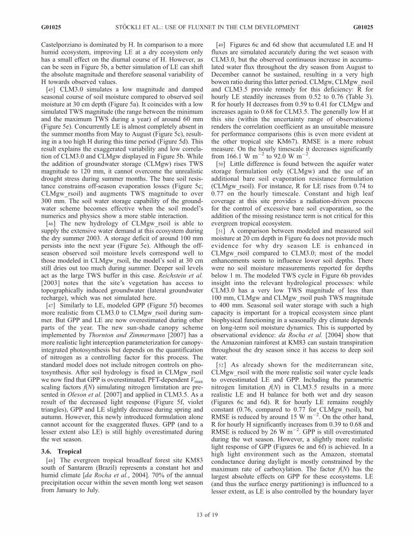
Table 1. Flux Towers Used in This Studya

Number Site Lon [�E] Lat [�N] Alt (Hgt) [m] Biome Type Soil Type Years Climate Zone

CarboEurope1 Vielsalm [Aubinet et al., 2001] 6.00 50.30 450 (40) MF loam 1997–2005 Temperate2 Tharandt [Grunwald and Bernhofer, 2007] 13.57 50.96 380 (42) ENF loam 1998–2003 Temperate3 Castel Porziano [Valentini, 2003] 12.38 41.71 68 (25) EBF loamy sand 2000–2005 Mediterranean4 Collelongo [Valentini, 2003] 13.59 41.85 1550 (32) DBF silt loam 1999–2003 Mediterranean5 Kaamanen [Laurila et al., 2001] 27.30 69.14 155 (5) TUN loam 2000–2005 North boreal6 Hyytiala [Suni et al., 2003] 24.29 61.85 181 (23) ENF loamy sand 1997–2005 Boreal7 El Saler [Ciais et al., 2005] �0.32 39.35 10 (15) ENF loamy sand 1999–2005 Mediterranean

LBA8 Santarem KM83 [Goulden et al., 2004] �54.97 �3.02 130 (64) EBF sandy clay 2001–2003 Tropical9 Tapajos KM67 [Hutyra et al., 2007] �54.96 �2.86 130 (63) EBF clay 2002–2005 Tropical

AmeriFlux10 Morgan Monroe [Schmid et al., 2000] �86.41 39.32 275 (46) DBF clay loam 1999–2005 Temperate11 Boreas OBS [Dunn et al., 2007] �98.48 55.88 259 (30) ENF clay loam 1994–2005 Boreal12 Lethbridge [Flanagan et al., 2002] �112.94 49.71 960 (4) GRA silt loam 1998–2004 Boreal13 Fort Peck [Gilmanov et al., 2005] �105.10 48.31 634 (4) GRA sandy loam 2000–2005 Temperate14 Harvard Forest [Urbanski et al., 2007] �72.17 42.54 303 (30) DBF sandy loam 1994–2003 Temperate15 Niwot Ridge [Monson et al., 2002] �105.55 40.03 3050 (26) ENF clay 1999–2004 SubalpineaBiome types: mixed forest (MF), evergreen needleleaf forest (ENF), deciduous broadleaf forest (DBF), tundra (TUN), evergreen broadleaf forest (EBF),

grasslands (GRA). Alt is the elevation of the tower above the sea level, and Hgt is the approximate height of the wind/temperature and flux measurementsabove the surface.


3 of 19

G01025

(Table 1) were used. Outliers which deviated ns times fromthe median-filtered time series were removed (s is thestandard deviation of the original time series and n = 4,except for RHa where n = 8; for u where n = 20 and for LWd

where n = 16). Up to two month long successive gaps werefilled by applying a 30 day running mean diurnal cycleforwards and backwards through the yearly time series.Years with more than 2 month of consecutive missing datawere not used.[15] The following exceptions were applied to the above

procedure:[16] 1. RGd was not median-filtered since most of its

variability occurs on diurnal timescale. Instead the potentialsolar radiation as a function of latitude and local solar time,scaled with the annual maximum observed RGd, providedan upper bound for RGd.[17] 2. P was neither median-filtered nor gap-filled.

Where provided by tower sites, daily precipitation totalsfrom nearby stations were used to replace missing 30 or60 min tower data. Daily precipitation totals were evenlydistributed at night between 00:00–04:00 during days whenno daily 30 or 60 min were available; and they were used toaugment valid 30 and 60 min data during days with partialmissing data periods.[18] 3. For sites with no Ps, it was estimated by

Ps ¼ Ps0e�Mgz

RTa ; ð1Þ

where Ps0is the mean sea level pressure (101300 Pa), M is

the molecular weight of air (0.029 kg mol�1), g is thegravitational acceleration (9.81 m s�2), z is the tower heightabove sea level (m) and R is the universal gas constant(8.314 J K�1 mol�1).[19] 4. For sites with no LWd (most sites), it was estimated

from the surface radiation balance:

LWd ¼ Rn � RGd þ RGu þ sTa þ Tr

2

� �4

; ð2Þ

where Rn and RGu are non-gap-filled net radiation (Wm�2)and upwelling solar radiation (Wm�2), s is the Stefan-Bolzmann constant (5.67 � 10�8 Wm�2K�4) and Tr is eitherthe canopy temperature or soil surface temperature (K),depending on data availability. As a backup algorithm (anyof the right hand side variables in equation (2) missing,most sites, again) downwelling long-wave radiation wasestimated by using the clear-sky LWd parameterization byIdso [1981], modified by an emissivity correction factor asproposed by Gabathuler et al. [2001]:

LWd ¼ �c�0sT4a ; ð3Þ

where:

�c ¼ 1þ 0:3 1� K0ð Þ2 and ð4Þ

�0 ¼ 0:7þ ea � 5:95 � 10�5e1500Ta ; ð5Þ

where �0 is the clear sky atmospheric emissivity as afunction of Ta and atmospheric vapor pressure ea (mb).�c adjusts �0 for cloud cover. It depends on the clearnessindex K0, which ranges from 0 to 1 (full cloud cover to clearsky). K0 can be approximated by dividing measured bypotential downwelling solar radiation, but only duringdaytime. We replaced all nocturnal K0 values where RGd

was below 50 W m�2 with linearly interpolated values.While clear sky LWd can be reasonably estimated the aboveformulation for all-sky LWd is a rough fix in need of somedata. Since cloud emissivity depends on, e.g., cloud type,water content and cloud vertical extent an uncertainty ofroughly 5–20 W m�2 is introduced to the driver data set[Gabathuler et al., 2001] by using this algorithm.[20] The consistently gap-filled meteorological forcing

data from the above 15 sites (and from around 50 additionalsites) are available from the authors (upon request also asALMA-compliant NetCDF files).2.2.2. Validation Data[21] Turbulent surface fluxes and soil physical state

variables from the Level 2 flux tower data sets were usedto validate the model during the implementation stage ofabove-described modifications. None of the validation datawere gap-filled since our intention was to look at timing andphase of the seasonal fluxes in response to climatic forcingsrather than to match the local-scale heat, water and carbonbalance at the end of the year. LE (latent heat flux; W m�2),H (sensible heat flux; W m�2), and NEE (net ecosystemexchange; mmol m�2 s�1) were u* filtered in order toaccount for the well documented biases in eddy covariancemeasurements during periods of low turbulence [Schmid etal., 2003]: comparisons to modeled fluxes were onlyperformed for times when the u* value was above 0.2 ms�1 (in the mean 67.4% of the data). Ideally, the u*threshold should be site-dependent and would only needto be applied to nocturnal data. Random uncertainties inturbulent surface fluxes [Hollinger and Richardson, 2005]were estimated based on empirical findings by Richardsonet al. [2006]. Systematic errors in measured surface fluxesdue to failure in energy balance closure were accounted forby multiplying u*-screened surface fluxes with the residualof the energy balance closure (as % of Rn) for each site, whichwas calculated from the regression of hourly observed Rn

versus LE and H fluxes [Wilson et al., 2002; Grunwald andBernhofer, 2007]. In all LE and H plots, the total errors werecalculated as the square root of the sum of the squares ofrandom and systematic errors for each analysis time step(e.g., hourly or monthly). Table 2 presents a summary ofthese uncertainty estimates for each site.[22] The model in its standard configuration simulates

GPP (gross primary productivity; mmol m�2 s�1) but not Re

(ecosystem respiration; mmol m�2 s�1). In order to calculateNEE (net ecosystem exchange; mmol m�2 s�1), which is thedifference between two large terms GPP and Re, both termswould need to be accurately prognosed. This requires amechanistic formulation involving prognostic carbon andnitrogen fluxes and pools as for instance presented byThornton et al. [2007]. In order to compare modeled carbonuptake to observations, observed estimates of GPP wereempirically derived from observed NEE, PAR (photosyn-thetically active radiation; mmol m�2 s�1), and Ts (5 cm soil


4 of 19

G01025

temperature; K) using the algorithms by Desai et al. [2005].Measured volumetric soil moisture was converted to percentsaturation by assuming a porosity of 0.48 and by using themodel soil layer which was closest to observation depth.

2.3. Experiment

[23] Single point model simulations were performed foreach of the 15 flux tower sites. The original model(CLM3.0) was successively modified with the proposedchanges:[24] 1. CLM3.0: the original and publicly available

release code of CLM3.0.[25] 2. CLMgw: addition of a Topmodel-based infiltra-

tion, runoff and aquifer storage formulation to CLM3.0.CLMgw (gw stands for groundwater) further includes allother major updates in the model (e.g., a new canopy

integration scheme, canopy interception changes, new fro-zen soil and plant soil water availability parameterizations)as described in Oleson et al. [2007] which were not part ofthe original CLM3.0.[26] 3. CLMgw_rsoil: addition of the bare soil evapora-

tion resistance formulation to CLMgw (rsoil stands for soilresistance).[27] 4. CLM3.5: addition of a PFT-dependent nitrogen

limitation factor to CLMgw_rsoil. This simulation is equiv-alent to the public release code of CLM3.5.2.3.1. Boundary Conditions[28] Vegetation and soil parameters for each site were

derived from the standard CLM3.0 PFT-dependent look-uptables based on vegetation type and soil type (constantvertical profiles of sand/clay fractions for each site) fromTable 1. A single PFT was used for each site. Visible and

Table 2. Uncertainty of Observations: % of u* Filtered Data (u*), % of Energy Balance Closure (ebc), Mean Error in LE Due to Failure

of Energy Balance Closure (ebc LE), Mean Random Error in LE (ran LE), Mean Error in H Due to Failure of Energy Balance Closure

(ebc H), and Mean Random Error in H (ran H)

Number Site u* % ebc % ebc LE W m�2 ran LE W m�2 ebc H W m�2 ran H W m�2

1 Vielsalm 21 73 7.0 20.2 7.5 29.72 Tharandt 44 78 8.4 24.5 7.7 29.83 Castel Porziano 34 83 8.6 25.7 13.9 36.64 Collelongo 41 81 8.8 28.1 12.3 37.15 Kaamanen 56 72 10.4 23.9 3.4 22.96 Hyytiala 47 72 8.3 21.5 6.2 26.17 El Saler 24 83 7.8 25.6 12.3 39.18 Santarem KM83 47 81 32.7 59.2 8.6 27.79 Tapajos KM67 36 81 24.9 44.9 6.5 26.310 Morgan Monroe 22 65 18.8 28.2 11.0 29.511 Boreas OBS 25 80 5.8 20.7 10.4 31.112 Lethbridge 42 77 7.3 21.8 8.8 34.313 Fort Peck 42 68 13.6 24.6 13.2 30.314 Harvard Forest 17 84 6.9 24.9 6.4 31.115 Niwot Ridge 17 76 12.7 27.6 12.3 40.7

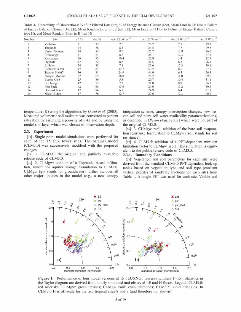
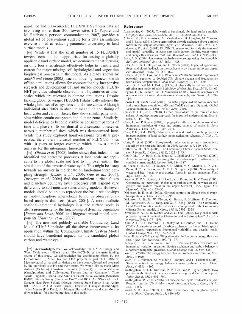
Figure 1. Performance of four model versions at 15 FLUXNET towers (numbers 1–15). Statistics inthe Taylor diagram are derived from hourly simulated and observed LE and H fluxes. Legend: CLM3.0:red asterisks; CLMgw: green crosses; CLMgw_rsoil: cyan diamonds; CLM3.5: violet triangles. InCLM3.0 H is off-scale for the two tropical sites 8 and 9 (and therefore not shown).


5 of 19

G01025

near-infrared soil albedos were set to arbitrary values of0.18/0.36 for a dry top soil and 0.09/0.18 for a saturated topsoil due to a lack of in-situ information at most sites. StemArea Index was set to 0.08. Vegetation top/bottom heightswere 35 m/1 m for tropical forests, 20m/10m for otherforests, and 1 m/0.1 m for short vegetation. A climatologicalmonthly Leaf Area Index for each site came from the 1982–2001 EFAI-NDVI data set [Stockli and Vidale, 2004]. Sinceour intent was to perform a process-based analysis of aglobal model, PFT-dependent model parameters were nottuned to site-specific and species-specific conditions.2.3.2. Initial Conditions and Spin-Up[29] The model was initialized from its standard arbitrary

initial conditions of 283 K vegetation, ground and soiltemperatures, 30% (CLM3.0) 40% (CLMgw, CLMgw_rsoil,CLM3.5) volumetric soil water content and with emptyground snow and canopy interception water stores. Spin-upwas achieved by repeating the full range of available yearsfive times for each site (five spin-up cycles). Mean yearlylatent and sensible heat fluxes were within 0.1 W m�2 ofthose from the previous spin-up cycle after a single spin-upcycle (similar to PILPS 2a spin-up criteria [Chen et al.,1997]). More arid climates would need longer spin-up timessince the water table there takes longer to adjust (see, e.g.,the global simulations by Oleson et al. [2008]). Neverthe-less, surface fluxes are not affected by variations of a verydeep water table in such areas.

2.3.3. Analysis[30] Hourly model output from the last spin-up cycle was

used for the analysis. At sites where 30 min measurementswere available they were averaged to 60 min values.

3. Results

[31] Comparisons between modeled and observed LE andH in Figure 1 (Taylor Diagram) and Table 3 (R and RMSE)provide a quick overview of performance changes acrossmodel versions: the original CLM3.0; modifications using agroundwater scheme (CLMgw), addition of a bare soilevaporation resistance (CLMgw_rsoil) and further additionof PFT-dependent nitrogen limitation factor in the finalmodel version (CLM3.5). (In the Taylor diagram [Taylor,2001], four statistical quantities are geometricallyconnected: the correlation coefficient R, standard deviationof observations so, standard deviation of the model sm, andthe centered pattern root-mean-square error E0. The polaraxis displays R and the radial axes display the standarddeviation of the modeled variable divided by the standarddeviation of the observed variable sm/so. The geometricrelationship of this diagram is such that the distancebetween the 1.0 value of the X-axis and the plotted valueshow E0 and thus is a measure for the absolute model error.Root-mean-square error E is given by: E = E + E0, where Eis the mean bias. The four statistical moments are connected

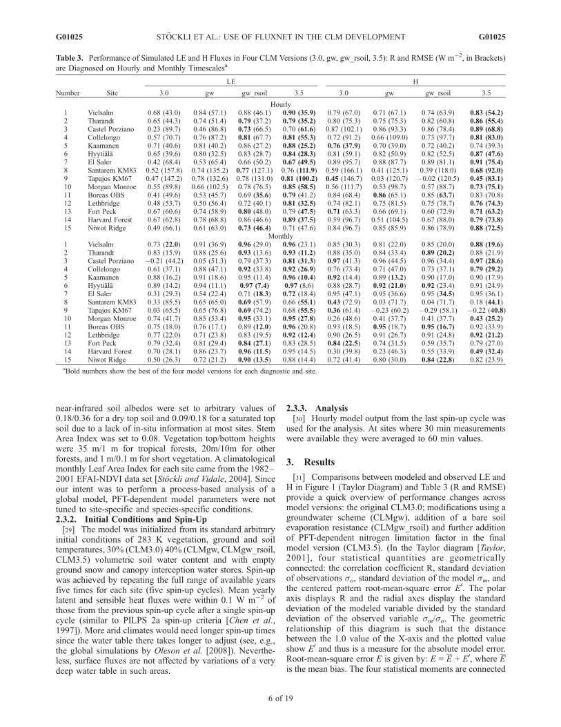
Table 3. Performance of Simulated LE and H Fluxes in Four CLM Versions (3.0, gw, gw_rsoil, 3.5): R and RMSE (W m�2, in Brackets)

are Diagnosed on Hourly and Monthly Timescalesa

Number Site

LE H

3.0 gw gw_rsoil 3.5 3.0 gw gw_rsoil 3.5

Hourly1 Vielsalm 0.68 (43.0) 0.84 (57.1) 0.88 (46.1) 0.90 (35.9) 0.79 (67.0) 0.71 (67.1) 0.74 (63.9) 0.83 (54.2)2 Tharandt 0.65 (44.3) 0.74 (51.4) 0.79 (37.2) 0.79 (35.2) 0.80 (75.3) 0.75 (75.3) 0.82 (60.8) 0.86 (55.4)3 Castel Porziano 0.23 (89.7) 0.46 (86.8) 0.73 (66.5) 0.70 (61.6) 0.87 (102.1) 0.86 (93.3) 0.86 (78.4) 0.89 (68.8)4 Collelongo 0.57 (70.7) 0.76 (87.2) 0.81 (67.7) 0.81 (55.3) 0.72 (91.2) 0.66 (109.0) 0.73 (97.7) 0.81 (83.0)5 Kaamanen 0.71 (40.6) 0.81 (40.2) 0.86 (27.2) 0.88 (25.2) 0.76 (37.9) 0.70 (39.0) 0.72 (40.2) 0.74 (39.3)6 Hyytiala 0.65 (39.6) 0.80 (32.5) 0.83 (28.7) 0.84 (28.3) 0.81 (59.1) 0.82 (50.9) 0.82 (52.5) 0.87 (47.6)7 El Saler 0.42 (68.4) 0.53 (65.4) 0.66 (50.2) 0.67 (49.5) 0.89 (95.7) 0.88 (87.7) 0.89 (81.1) 0.91 (75.4)8 Santarem KM83 0.52 (157.8) 0.74 (135.2) 0.77 (127.1) 0.76 (111.9) 0.59 (166.1) 0.41 (125.1) 0.39 (118.0) 0.68 (92.0)9 Tapajos KM67 0.47 (147.2) 0.78 (132.6) 0.78 (131.0) 0.81 (100.2) 0.45 (146.7) 0.03 (120.7) �0.02 (120.5) 0.45 (83.1)10 Morgan Monroe 0.55 (89.8) 0.66 (102.5) 0.78 (76.5) 0.85 (58.5) 0.56 (111.7) 0.53 (98.7) 0.57 (88.7) 0.73 (75.1)11 Boreas OBS 0.41 (49.6) 0.53 (45.7) 0.69 (35.6) 0.79 (41.2) 0.84 (68.4) 0.86 (65.1) 0.85 (63.7) 0.83 (70.8)12 Lethbridge 0.48 (53.7) 0.50 (56.4) 0.72 (40.1) 0.81 (32.5) 0.74 (82.1) 0.75 (81.5) 0.75 (78.7) 0.76 (74.3)13 Fort Peck 0.67 (60.6) 0.74 (58.9) 0.80 (48.0) 0.79 (47.5) 0.71 (63.3) 0.66 (69.1) 0.60 (72.9) 0.71 (63.2)14 Harvard Forest 0.67 (62.8) 0.78 (68.8) 0.86 (46.6) 0.89 (37.5) 0.59 (96.7) 0.51 (104.5) 0.67 (88.0) 0.79 (73.8)15 Niwot Ridge 0.49 (66.1) 0.61 (63.0) 0.73 (46.4) 0.71 (47.6) 0.84 (96.7) 0.85 (85.9) 0.86 (78.9) 0.88 (72.5)

Monthly1 Vielsalm 0.73 (22.0) 0.91 (36.9) 0.96 (29.0) 0.96 (23.1) 0.85 (30.3) 0.81 (22.0) 0.85 (20.0) 0.88 (19.6)2 Tharandt 0.83 (15.9) 0.88 (25.6) 0.93 (13.6) 0.93 (11.2) 0.88 (35.0) 0.84 (33.4) 0.89 (20.2) 0.88 (21.9)3 Castel Porziano �0.21 (44.2) 0.05 (51.3) 0.79 (37.3) 0.81 (31.3) 0.97 (41.3) 0.96 (44.5) 0.96 (34.4) 0.97 (28.6)4 Collelongo 0.61 (37.1) 0.88 (47.1) 0.92 (33.8) 0.92 (26.9) 0.76 (73.4) 0.71 (47.0) 0.73 (37.1) 0.79 (29.2)5 Kaamanen 0.88 (16.2) 0.91 (18.6) 0.95 (11.4) 0.96 (10.4) 0.92 (14.4) 0.89 (13.2) 0.90 (17.0) 0.90 (17.9)6 Hyytiala 0.89 (14.2) 0.94 (11.1) 0.97 (7.4) 0.97 (8.6) 0.88 (28.7) 0.92 (21.0) 0.92 (23.4) 0.91 (24.9)7 El Saler 0.31 (29.3) 0.54 (22.4) 0.71 (18.3) 0.72 (18.4) 0.95 (47.1) 0.95 (36.6) 0.95 (34.5) 0.95 (36.1)8 Santarem KM83 0.33 (85.5) 0.65 (65.0) 0.69 (57.9) 0.66 (55.1) 0.43 (72.9) 0.03 (71.7) 0.04 (71.7) 0.18 (44.1)9 Tapajos KM67 0.03 (65.5) 0.65 (76.8) 0.69 (74.2) 0.68 (55.5) 0.36 (61.4) �0.23 (60.2) �0.29 (58.1) �0.22 (40.8)10 Morgan Monroe 0.74 (41.7) 0.85 (53.4) 0.95 (33.1) 0.95 (27.8) 0.26 (48.6) 0.41 (37.7) 0.41 (37.7) 0.43 (25.2)11 Boreas OBS 0.75 (18.0) 0.76 (17.1) 0.89 (12.0) 0.96 (20.8) 0.93 (18.5) 0.95 (18.7) 0.95 (16.7) 0.92 (33.9)12 Lethbridge 0.77 (22.0) 0.71 (23.8) 0.83 (19.5) 0.92 (12.4) 0.90 (26.5) 0.91 (26.7) 0.91 (24.8) 0.92 (21.2)13 Fort Peck 0.79 (32.4) 0.81 (29.4) 0.84 (27.1) 0.83 (28.5) 0.84 (22.5) 0.74 (31.5) 0.59 (35.7) 0.79 (27.0)14 Harvard Forest 0.70 (28.1) 0.86 (23.7) 0.96 (11.5) 0.95 (14.5) 0.30 (39.8) 0.23 (46.3) 0.55 (33.9) 0.49 (32.4)15 Niwot Ridge 0.50 (26.3) 0.72 (21.2) 0.90 (13.5) 0.88 (14.4) 0.72 (41.4) 0.80 (30.0) 0.84 (22.8) 0.82 (23.9)aBold numbers show the best of the four model versions for each diagnostic and site.


6 of 19

G01025

by: E02 = sm2 + so

2 � 2smsoR.) General changes in LE and Hon the hourly and monthly timescale covering all sites arediscussed first, followed by a close inspection of results atindividual sites encompassing temperate, north boreal,mediterranean and the tropical ecosystems.

3.1. Latent Heat Flux

[32] The R of LE shown in Figure 1a increases with thenew groundwater scheme (CLMgw, green crosses) com-pared to the original CLM3.0 (red asterisks). However, thevariability of LE is now exaggerated compared to observa-tions. The inclusion of the bare soil evaporation resistance(CLMgw_rsoil, cyan diamonds) generates more realistic LEvariability, resulting in a higher R than with the groundwa-ter formulation alone. A further improvement in bothcorrelation and variability is achieved with the nitrogenlimitation (CLM3.5, violet triangles). R for hourly LE atmost sites increases from around 0.4–0.7 (CLM3.0) and0.5 – 0.8 (CLMgw) to 0.7 – 0.9 (CLMgw_rsoil andCLM3.5). For all 15 sites hourly and monthly LE has ahigher R and a lower RMSE for CLM3.5 compared toCLM3.0. Some sites display substantial improvements: e.g.,the mediterranean site Castelporziano (R increases from0.23 to 0.70 for hourly LE and from �0.21 to 0.81 formonthly LE) and the tropical site KM67 (R for hourly LEincreases from 0.47 to 0.81; and for monthly LE from 0.03to 0.68). Similarly, temperate ecosystems show a steadyimprovement (e.g., Vielsalm or Morgan Monroe). Highlatitude ecosystems (e.g., Kaamanen and Hyytiala) arealready well simulated by CLM3.0, but they also slightlyimprove. RMSE decreases at all sites (except for Vielsalm atthe monthly timescale) from CLM3.0 to CLM3.5 on bothhourly and monthly timescale. The grassland sites Leth-bridge and Fort Peck improve on both hourly and monthlytimescale, but to a lesser extent than forest sites.

3.2. Sensible Heat Flux

[33] The changes in H, shown in Figure 1b, are not aseasily generalized as LE, although the model changesappear to result in an overall improvement. Even thoughchanges in LE are almost fully compensated by oppositechanges in H, the new hydrology formulations do not affectR of H as much. This is due to a number of factors. First ofall, H is smaller than LE for most sites. Secondly, while LEcan completely be shut down by soil moisture, H is stronglycoupled to net shortwave radiation through skin tempera-ture, largely independent of the state of subsurface hydrol-ogy [Betts, 2004]. R is a good indicator for phase but not formagnitude in this case. For sites like Castelporziano, wherethe R of LE increased substantially, R of H remains constant(R increases from 0.87 to 0.89; hourly timescale). ButRMSE of H decreases from 102.1 W m�2 to 68.8 W m�2.Remaining high RMSE values should also be viewed withrespect to uncertainties in observed fluxes (Table 2). Thisresult suggests that the mean error and variability of H wasimproved with the new hydrology, and not the timing andphase of H. Indeed, in Figure 1b R values remain roughlythe same for all four model versions. But the spread in theradial direction decreases and successively moves symbolscloser towards observed variability at the 1.0 arc by use ofthe new formulations. Several sites actually show a slightlyworse R with the new hydrology, but they still have a

decreased RMSE compared to CLM3.0. For the two tropicalsites hourly R for H becomes worse in CLMgw andCLMgw_rsoil and increases again with CLM3.5. Hourlyand monthly RMSE for those sites significantly decreasesby around 35–45%. Only small changes in R and RMSE onboth hourly and monthly timescale can be seen for the twograsslands Fort Peck and Lethbridge. They cannot make useof the groundwater if the water table falls below theirshallow rooting depth, which is most likely the case atthose two sites.

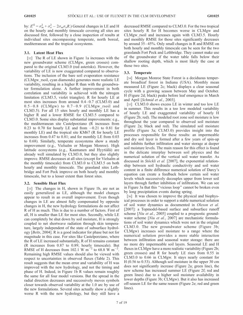
3.3. Temperate

[34] Morgan Monroe State Forest is a deciduous temper-ate broadleaf forest in Indiana (USA). Monthly meanmeasured LE (Figure 2c; black) displays a clear seasonalcycle with a growing season between May and October.H (Figure 2d; black) peaks before leaf emergence in Marchand April [Schmid et al., 2003].[35] CLM3.0 shows excess LE in winter and too low LE

in summer. This results in a too low modeled variabilityof hourly LE and exaggerated variability of hourly H(Figure 2b; red). The modeled root zone soil moisture is lowthroughout the year compared to observed soil moisture(Figure 2a; black and red). The simulated soil moistureprofile (Figure 3a; CLM3.0) provides insight into theprocesses responsible for these results: an impermeableand dry soil layer is formed after a few years of spin-upand inhibits further infiltration and water storage at deepersoil moisture levels. The main reason for this effect is foundin the delicate interplay between soil physics and thenumerical solution of the vertical soil water transfer. Asdiscussed in Stockli et al. [2007], the exponential relation-ship between soil hydraulic conductivity and soil watercontent in a finite difference numerical solution of Darcy’sequation can create a feedback below certain soil waterlevels which successively decouples upper from lower soillayers through further inhibition of infiltration. We can seein Figure 3a that this ‘‘vicious loop’’ cannot be broken evenby long precipitation events during spring.[36] It was chosen to improve the physical and biophys-

ical processes in order to support a stable numerical solutionof soil water dynamics as documented in Oleson et al.[2007]: a Topmodel-based surface and subsurface runoffscheme [Niu et al., 2005] coupled to a prognostic ground-water scheme [Niu et al., 2007] are mechanistic formula-tions of soil water dynamics which were not in the originalCLM3.0. The new groundwater scheme (Figure 3b;CLMgw) increases soil moisture to a range where thenumerical solution provides a more stable interactionbetween infiltration and seasonal water storage: there areno more dry impermeable soil layers. Seasonal LE and Hfluxes in CLMgw have amore realistic variability (Figure 2b;green crosses) and R for hourly LE rises from 0.55 inCLM3.0 to 0.66 in CLMgw. It stays nearly constant forH (0.56 to 0.53). Although soil moisture in the upper 30 cmdoes not significantly increase (Figure 2a; green line), thenew scheme has increased summer LE (Figure 2f; red andgreen lines) due to a higher soil moisture availability inlower depths (Figure 3b; CLMgw). But it also has increasedoff-season LE for the same reason (Figure 2e; red and greenlines).


7 of 19

G01025

Figure 2. Model diagnostics at a temperate deciduous forest (Morgan Monroe State Forest, USA)during 2003: (a) soil moisture relative to saturation at 30 cm depth; (b) Taylor diagram with hourlystatistics of LE and H fluxes; (c) monthly LE fluxes; (d) monthly H fluxes; (e) diurnal cycle of LE fluxesin February; (f) diurnal cycle of LE fluxes in August. Error bars show estimated uncertainties of observedturbulent fluxes. Legend: observations: black plus signs; CLM3.0: red asterisks; CLMgw: green crosses;CLMgw_rsoil: cyan diamonds; CLM3.5: violet triangles.


8 of 19

G01025

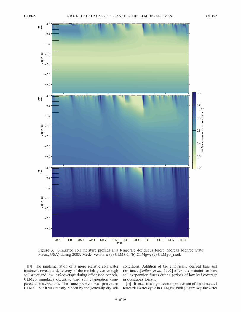
[37] The implementation of a more realistic soil watertreatment reveals a deficiency of the model: given enoughsoil water and low leaf-coverage during off-season periods,CLMgw simulates excessive bare soil evaporation com-pared to observations. The same problem was present inCLM3.0 but it was mostly hidden by the generally dry soil

conditions. Addition of the empirically derived bare soilresistance [Sellers et al., 1992] offers a constraint for baresoil evaporation fluxes during periods of low leaf coveragein deciduous forests.[38] It leads to a significant improvement of the simulated

terrestrial water cycle in CLMgw_rsoil (Figure 3c): the water

Figure 3. Simulated soil moisture profiles at a temperate deciduous forest (Morgan Monroe StateForest, USA) during 2003. Model versions: (a) CLM3.0; (b) CLMgw; (c) CLMgw_rsoil.


9 of 19

G01025

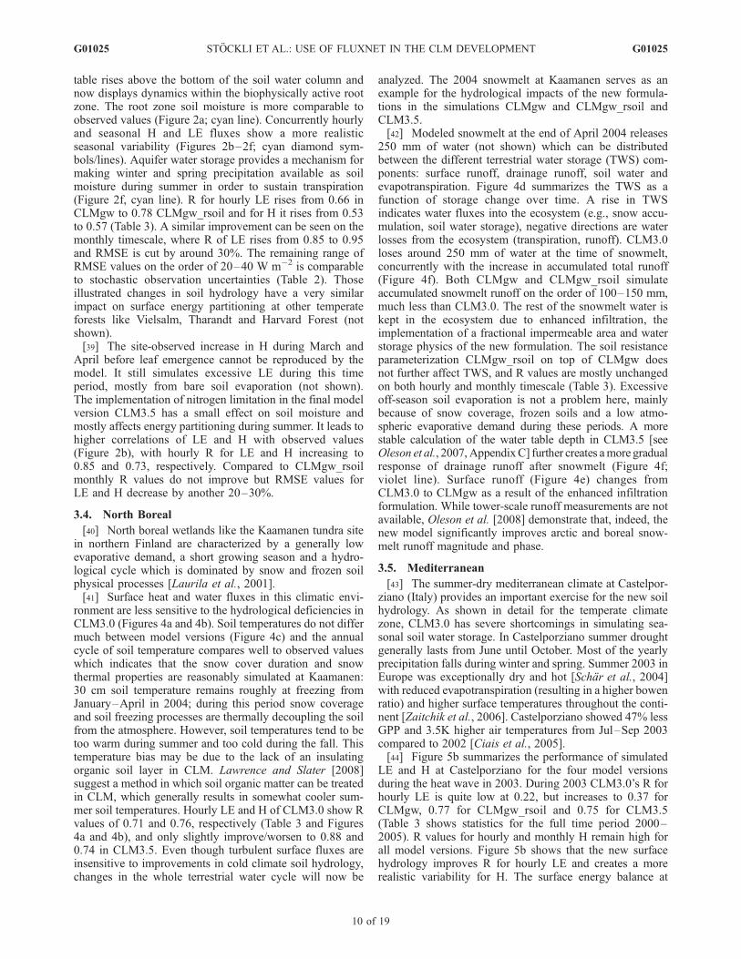
table rises above the bottom of the soil water column andnow displays dynamics within the biophysically active rootzone. The root zone soil moisture is more comparable toobserved values (Figure 2a; cyan line). Concurrently hourlyand seasonal H and LE fluxes show a more realisticseasonal variability (Figures 2b–2f; cyan diamond sym-bols/lines). Aquifer water storage provides a mechanism formaking winter and spring precipitation available as soilmoisture during summer in order to sustain transpiration(Figure 2f, cyan line). R for hourly LE rises from 0.66 inCLMgw to 0.78 CLMgw_rsoil and for H it rises from 0.53to 0.57 (Table 3). A similar improvement can be seen on themonthly timescale, where R of LE rises from 0.85 to 0.95and RMSE is cut by around 30%. The remaining range ofRMSE values on the order of 20–40 W m�2 is comparableto stochastic observation uncertainties (Table 2). Thoseillustrated changes in soil hydrology have a very similarimpact on surface energy partitioning at other temperateforests like Vielsalm, Tharandt and Harvard Forest (notshown).[39] The site-observed increase in H during March and

April before leaf emergence cannot be reproduced by themodel. It still simulates excessive LE during this timeperiod, mostly from bare soil evaporation (not shown).The implementation of nitrogen limitation in the final modelversion CLM3.5 has a small effect on soil moisture andmostly affects energy partitioning during summer. It leads tohigher correlations of LE and H with observed values(Figure 2b), with hourly R for LE and H increasing to0.85 and 0.73, respectively. Compared to CLMgw_rsoilmonthly R values do not improve but RMSE values forLE and H decrease by another 20–30%.

3.4. North Boreal

[40] North boreal wetlands like the Kaamanen tundra sitein northern Finland are characterized by a generally lowevaporative demand, a short growing season and a hydro-logical cycle which is dominated by snow and frozen soilphysical processes [Laurila et al., 2001].[41] Surface heat and water fluxes in this climatic envi-

ronment are less sensitive to the hydrological deficiencies inCLM3.0 (Figures 4a and 4b). Soil temperatures do not differmuch between model versions (Figure 4c) and the annualcycle of soil temperature compares well to observed valueswhich indicates that the snow cover duration and snowthermal properties are reasonably simulated at Kaamanen:30 cm soil temperature remains roughly at freezing fromJanuary–April in 2004; during this period snow coverageand soil freezing processes are thermally decoupling the soilfrom the atmosphere. However, soil temperatures tend to betoo warm during summer and too cold during the fall. Thistemperature bias may be due to the lack of an insulatingorganic soil layer in CLM. Lawrence and Slater [2008]suggest a method in which soil organic matter can be treatedin CLM, which generally results in somewhat cooler sum-mer soil temperatures. Hourly LE and H of CLM3.0 show Rvalues of 0.71 and 0.76, respectively (Table 3 and Figures4a and 4b), and only slightly improve/worsen to 0.88 and0.74 in CLM3.5. Even though turbulent surface fluxes areinsensitive to improvements in cold climate soil hydrology,changes in the whole terrestrial water cycle will now be

analyzed. The 2004 snowmelt at Kaamanen serves as anexample for the hydrological impacts of the new formula-tions in the simulations CLMgw and CLMgw_rsoil andCLM3.5.[42] Modeled snowmelt at the end of April 2004 releases

250 mm of water (not shown) which can be distributedbetween the different terrestrial water storage (TWS) com-ponents: surface runoff, drainage runoff, soil water andevapotranspiration. Figure 4d summarizes the TWS as afunction of storage change over time. A rise in TWSindicates water fluxes into the ecosystem (e.g., snow accu-mulation, soil water storage), negative directions are waterlosses from the ecosystem (transpiration, runoff). CLM3.0loses around 250 mm of water at the time of snowmelt,concurrently with the increase in accumulated total runoff(Figure 4f). Both CLMgw and CLMgw_rsoil simulateaccumulated snowmelt runoff on the order of 100–150 mm,much less than CLM3.0. The rest of the snowmelt water iskept in the ecosystem due to enhanced infiltration, theimplementation of a fractional impermeable area and waterstorage physics of the new formulation. The soil resistanceparameterization CLMgw_rsoil on top of CLMgw doesnot further affect TWS, and R values are mostly unchangedon both hourly and monthly timescale (Table 3). Excessiveoff-season soil evaporation is not a problem here, mainlybecause of snow coverage, frozen soils and a low atmo-spheric evaporative demand during these periods. A morestable calculation of the water table depth in CLM3.5 [seeOleson et al., 2007, AppendixC] further creates amore gradualresponse of drainage runoff after snowmelt (Figure 4f;violet line). Surface runoff (Figure 4e) changes fromCLM3.0 to CLMgw as a result of the enhanced infiltrationformulation. While tower-scale runoff measurements are notavailable, Oleson et al. [2008] demonstrate that, indeed, thenew model significantly improves arctic and boreal snow-melt runoff magnitude and phase.

3.5. Mediterranean

[43] The summer-dry mediterranean climate at Castelpor-ziano (Italy) provides an important exercise for the new soilhydrology. As shown in detail for the temperate climatezone, CLM3.0 has severe shortcomings in simulating sea-sonal soil water storage. In Castelporziano summer droughtgenerally lasts from June until October. Most of the yearlyprecipitation falls during winter and spring. Summer 2003 inEurope was exceptionally dry and hot [Schar et al., 2004]with reduced evapotranspiration (resulting in a higher bowenratio) and higher surface temperatures throughout the conti-nent [Zaitchik et al., 2006]. Castelporziano showed 47% lessGPP and 3.5K higher air temperatures from Jul–Sep 2003compared to 2002 [Ciais et al., 2005].[44] Figure 5b summarizes the performance of simulated

LE and H at Castelporziano for the four model versionsduring the heat wave in 2003. During 2003 CLM3.0’s R forhourly LE is quite low at 0.22, but increases to 0.37 forCLMgw, 0.77 for CLMgw_rsoil and 0.75 for CLM3.5(Table 3 shows statistics for the full time period 2000–2005). R values for hourly and monthly H remain high forall model versions. Figure 5b shows that the new surfacehydrology improves R for hourly LE and creates a morerealistic variability for H. The surface energy balance at


10 of 19

G01025

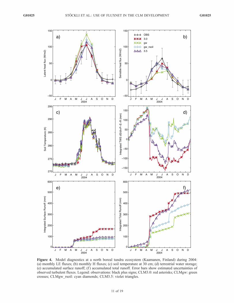
Figure 4. Model diagnostics at a north boreal tundra ecosystem (Kaamanen, Finland) during 2004:(a) monthly LE fluxes; (b) monthly H fluxes; (c) soil temperature at 30 cm; (d) terrestrial water storage;(e) accumulated surface runoff; (f ) accumulated total runoff. Error bars show estimated uncertainties ofobserved turbulent fluxes. Legend: observations: black plus signs; CLM3.0: red asterisks; CLMgw: greencrosses; CLMgw_rsoil: cyan diamonds; CLM3.5: violet triangles.


11 of 19

G01025

Figure 5. Model diagnostics at a mediterranean hardwood forest (Castel Porziano, Italy) for 2003:(a) soil moisture at 30 cm depth; (b) Taylor diagram showing statistics from hourly LE and H fluxes;(c) monthly LE fluxes; (d) monthly H fluxes; (e) terrestrial water storage; (f ) modeled versus NEE-derived GPP. Error bars show estimated uncertainties of observed turbulent fluxes. Legend: observations:black plus signs; CLM3.0: red asterisks; CLMgw: green crosses; CLMgw_rsoil: cyan diamonds;CLM3.5: violet triangles.


12 of 19

G01025

Castelporziano is dominated by H. In comparison to a morehumid ecosystem, improving LE at a dry ecosystem onlyhas a small effect on the diurnal course of H. However, ascan be seen in Figure 5b, a better simulation of LE can shiftthe absolute magnitude and therefore seasonal variability ofH towards observed values.[45] CLM3.0 simulates a low magnitude and damped

seasonal course of soil moisture compared to observed soilmoisture at 30 cm depth (Figure 5a). It coincides with a lowsimulated TWS magnitude (the range between the minimumand the maximum TWS during a year) of around 60 mm(Figure 5e). Concurrently LE is almost completely absent inthe summer months from May to August (Figure 5c), result-ing in a too high H during this time period (Figure 5d). Thisresult explains the exaggerated variability and low correla-tion of CLM3.0 and CLMgw displayed in Figure 5b. Whilethe addition of groundwater storage (CLMgw) rises TWSmagnitude to 120 mm, it cannot overcome the unrealisticdrought stress during summer months. The bare soil resis-tance constrains off-season evaporation losses (Figure 5c;CLMgw_rsoil) and augments TWS magnitude to over300 mm. The soil water storage capability of the ground-water scheme becomes effective when the soil model’snumerics and physics show a more stable interaction.[46] The new hydrology of CLMgw_rsoil is able to

supply the extensive water demand at this ecosystem duringthe dry summer 2003. A storage deficit of around 100 mmpersists into the next year (Figure 5e). Although the off-season observed soil moisture levels correspond well tothose modeled in CLMgw_rsoil, the model’s soil at 30 cmstill dries out too much during summer. Deeper soil levelsact as the large TWS buffer in this case. Reichstein et al.[2003] notes that the site’s vegetation has access totopographically induced groundwater (lateral groundwaterrecharge), which was not simulated here.[47] Similarly to LE, modeled GPP (Figure 5f) becomes

more realistic from CLM3.0 to CLMgw_rsoil during sum-mer. But GPP and LE are now overestimated during otherparts of the year. The new sun-shade canopy schemeimplemented by Thornton and Zimmermann [2007] has amore realistic light interception parameterization for canopy-integrated photosynthesis but depends on the quantificationof nitrogen as a controlling factor for this process. Thestandard model does not include nitrogen controls on pho-tosynthesis. After soil hydrology is fixed in CLMgw_rsoilwe now find that GPP is overestimated. PFT-dependent Vmax

scaling factors f(N) simulating nitrogen limitation are pre-sented in Oleson et al. [2007] and applied in CLM3.5. As aresult of the decreased light response (Figure 5f, violettriangles), GPP and LE slightly decrease during spring andautumn. However, this newly introduced formulation alonecannot account for the exaggerated fluxes. GPP (and to alesser extent also LE) is still highly overestimated duringthe wet season.

3.6. Tropical

[48] The evergreen tropical broadleaf forest site KM83south of Santarem (Brazil) represents a constant hot andhumid climate [da Rocha et al., 2004]. 70% of the annualprecipitation occur within the seven month long wet seasonfrom January to July.

[49] Figures 6c and 6d show that accumulated LE and Hfluxes are simulated accurately during the wet season withCLM3.0, but the observed continuous increase in accumu-lated water flux throughout the dry season from August toDecember cannot be sustained, resulting in a very highbowen ratio during this latter period. CLMgw, CLMgw_rsoiland CLM3.5 provide remedy for this deficiency: R forhourly LE steadily increases from 0.52 to 0.76 (Table 3).R for hourly H decreases from 0.59 to 0.41 for CLMgw andincreases again to 0.68 for CLM3.5. The generally low H atthis site (within the uncertainty range of observations)renders the correlation coefficient as an unsuitable measurefor performance comparisons (this is even more evident atthe other tropical site KM67). RMSE is a more robustmeasure. On the hourly timescale it decreases significantlyfrom 166.1 W m�2 to 92.0 W m�2.[50] Little difference is found between the aquifer water

storage formulation only (CLMgw) and the use of anadditional bare soil evaporation resistance formulation(CLMgw_rsoil). For instance, R for LE rises from 0.74 to0.77 on the hourly timescale. Constant and high leafcoverage at this site provides a radiation-driven processfor the control of excessive bare soil evaporation, so theaddition of the missing resistance term is not critical for thisevergreen tropical ecosystem.[51] A comparison between modeled and measured soil

moisture at 20 cm depth in Figure 6a does not provide muchevidence for why dry season LE is enhanced inCLMgw_rsoil compared to CLM3.0; most of the modelenhancements seem to influence lower soil depths. Therewere no soil moisture measurements reported for depthsbelow 1 m. The modeled TWS cycle in Figure 6b providesinsight into the relevant hydrological processes: whileCLM3.0 has a very low TWS magnitude of less than100 mm, CLMgw and CLMgw_rsoil push TWS magnitudeto 400 mm. Seasonal soil water storage with such a highcapacity is important for a tropical ecosystem since plantbiophysical functioning in a seasonally dry climate dependson long-term soil moisture dynamics. This is supported byobservational evidence: da Rocha et al. [2004] show thatthe Amazonian rainforest at KM83 can sustain transpirationthroughout the dry season since it has access to deep soilwater.[52] As already shown for the mediterranean site,

CLMgw_rsoil with the more realistic soil water cycle leadsto overestimated LE and GPP. Including the parametricnitrogen limitation f(N) in CLM3.5 results in a morerealistic LE and H balance for both wet and dry season(Figures 6c and 6d). R for hourly LE remains roughlyconstant (0.76, compared to 0.77 for CLMgw_rsoil), butRMSE is reduced by around 15 W m�2. On the other hand,R for hourly H significantly increases from 0.39 to 0.68 andRMSE is reduced by 26 W m�2. GPP is still overestimatedduring the wet season. However, a slightly more realisticlight response of GPP (Figures 6e and 6f) is achieved. In ahigh light environment such as the Amazon, stomatalconductance during daylight is mostly constrained by themaximum rate of carboxylation. The factor f(N) has thelargest absolute effects on GPP for these ecosystems. LE(and thus the surface energy partitioning) is influenced to alesser extent, as LE is also controlled by the boundary layer


13 of 19

G01025

Figure 6. Model diagnostics at a tropical evergreen forest (Santarem KM83, Brazil) during 2002:(a) soil moisture at 20 cm depth; (b) terrestrial water storage; (c) accumulated LE fluxes; (d) accumulatedH fluxes; (e) modeled versus NEE-derived GPP; (f ) mean light response curves for modeled and NEE-derived GPP (binned by incoming solar radiation). Error bars show estimated uncertainties of observedturbulent fluxes. Legend: observations: black plus signs; CLM3.0: red asterisks; CLMgw: green crosses;CLMgw_rsoil: cyan diamonds; CLM3.5: violet triangles.


14 of 19

G01025

vapor pressure gradient, bare soil evaporation and aerody-namical properties.

4. Discussion

[53] Turbulent heat and water fluxes of the originalCLM3.0 show significant biases in tropical, mediterraneanand temperate climatic environments. These biases resultfrom a poor representation of soil moisture storage and itsinteraction with seasonal variations of the surface climate.Modeled plant transpiration generally shuts down duringeither summer or dry seasons due to a lack of soil moisturesupply. Observations from the 15 flux tower sites, however,indicate that plants can sustain their physiological functionduring seasonal-scale and longer term drought periods.Subsurface hydrological processes on which these plantslargely depend therefore need to be properly represented inland surface models in order to simulate the terrestrialcarbon and water cycle [Reichstein et al., 2002]. Thisrequirement gains further importance in view of the pre-dicted temperature and precipitation changes in future cli-mate scenarios, which could severely affect ecosystemfunction during hotter and drier summer periods [Seneviratneet al., 2006].

4.1. Terrestrial Water Storage

[54] To achieve a higher water storage capacity in a landsurface model, the total soil depth and other soil parametersare often modified as a first guess. The above findings,however, suggest that soil water storage capacity is adynamic quantity. It does not primarily depend on soilphysical parameters. It rather results from a consistentinterplay between the soil and vegetation biophysicalparameterizations on one side and the soil numericalscheme on the other side: they both depend on each otherin order to provide a realistic simulation of the terrestrialwater cycle.[55] At the mediterranean and temperate sites only small

improvements in surface fluxes result from the implemen-tation of larger soil water storage capacity by use of aprognostic aquifer scheme. Soil water infiltration and stor-age are both still largely inhibited by excessive bare soilevaporation during off-season periods in those ecosystems.Further addition of a bare soil evaporation resistance finallyresults in a realistic TWS magnitude and concurrently in asubstantial increase of turbulent flux R and decrease inRMSE at most sites. Figures 3a–3c illustrate the underlyingsoil hydrological processes:[56] 1. A dry soil can continuously inhibit vertical soil

moisture fluxes and thus decrease seasonal water storage byhydrologically decoupling upper from lower soil layers.[57] 2. Extending the storage pool by implementing a

prognostic aquifer breaks the infiltration barrier by provid-ing ample soil moisture to the root zone but TWS remains ata low seasonal magnitude (e.g., Figure 5e).[58] 3. Bare soil evaporation during off-season periods

was identified as the main process which dampens TWSmagnitude for deciduous vegetation in temperate and med-iterranean climate zones. With a more realistic off-seasonbare soil evaporation TWS becomes positive during thewinter or wet season when moisture is stored in the soil. Asa consequence transpiration fluxes during months of low

rainfall (dry season) or large atmospheric demands (summerseason) substantially improve.[59] While a prognostic aquifer model [Niu et al., 2005,

2007] provides the physical framework for simulating largeseasonal TWS fluctuations, the size of TWS magnitudedepends on a dynamically varying set of involved soil andvegetation processes. The new hydrological formulationsenhance TWS by 200–300 mm compared to the originalCLM3.0, with quite beneficial effects for the simulatedsurface energy and water balances in seasonally dry cli-mates. This result is highly consistent with comparisonsbetween modeled and GRACE estimates of TWS at catch-ment scale presented by Oleson et al. [2008]. They showthat CLM3.5 enhances TWS magnitude by 50–300 mmcompared to CLM3.0, with improved correlations andsubstantial decreases in RMSE.[60] In northern boreal regions like Kaamanen, however,

TWS magnitude decreases by around 100 mm whengroundwater storage is added (Figure 4e). This behavior isopposite to what one would expect. As in warm climates,soil water storage function of cold climates not onlydepends on storage capacity, but closely interacts with thedominant hydrological processes through time-delayedfeedbacks: the analysis shows that snowmelt water can bestored in spring after soil thaw and should not completelyrun off into rivers like in the original formulation. Soilmoisture storage seems to dampen the seasonal course ofTWS at Kaamanen. While adding groundwater does notmuch affect turbulent surface fluxes in cold climates(Figures 4a and 4b) it could lead to improvements in highlatitude runoff timing and magnitude (Figures 4e and 4f).This is documented in Oleson et al. [2008] by comparisonof global simulated versus observed river discharge andrunoff.

4.2. Nitrogen Limitation

[61] Results from the mediterranean and tropical sitessuggest that the enhanced and more realistic water storageprocesses in the model can lead to excessive transpiration.The addition of a parameterized nitrogen control for pho-tosynthesis decreases light sensitivity of stomatal openingas expected (Figures 5f, 6e, and 6f). The need for thisparameterization only became evident after the new soilhydrology and the new canopy integration scheme wasimplemented: maximum photosynthesis rates in CLM3.0were fixed, based on observed values. Low soil moisturelevels furthermore limited the plant physiological activity inmost climates. Parameterized nitrogen control became anecessity with the new hydrological modifications. Whilenitrogen is an important controlling factor for most terres-trial ecosystems (f(N) ranging from 0.60–0.84 in Oleson etal. [2007]), our results suggest that it mostly affects thesurface energy and water balance in environments with highGPP. Tropical broadleaf forests have the lowest diagnosednitrogen limitations among the 16 PFTs (highest f(N) =0.84). However, they mostly operate at high light levels,resulting in the largest nitrogen-controlled decreases in GPPin absolute terms. In comparison to GPP, LE is less sensitiveto changes in stomatal conductance through nitrogen controlbecause LE is a composite of transpiration and bare soilevaporation. The latter is independent of nitrogen availabil-ity. LE is further controlled by boundary layer aerodynamical


15 of 19

G01025

resistances, which only indirectly and weakly influenceGPP. Nevertheless, results show a positive effect of thenewly introduced f(N) on R and RMSE of hourly andmonthly LE and H fluxes. The two tropical sites KM67and KM83 show the largest decrease in RMSE (Table 3) byincluding f(N) compared to simulations with changes in soilhydrology alone. Boundary layer processes for these eco-systems are expected to benefit from this model enhance-ment in coupled simulations.

4.3. Open Questions

[62] Figures 5f and 6f show that yet another processmight be missing. LE and GPP are still overestimatedduring the wet season at the mediterranean and the tropicalsite. LE is less of a problem than GPP since LE is alsodriven by the atmospheric vapor pressure gradient andsurface layer aerodynamics. It furthermore is compositedfrom plant transpiration and bare soil evaporation, the latterbeing unrelated to stomatal functioning. Suggestions formissing processes are, e.g., a prognostic dry season phe-nology (which can also vary in tropical ecosystems [Myneniet al., 2007]) and dynamic allocation of leaf structure andphotosynthates [Dickinson et al., 2002], which are notsimulated in the standard CLM. Simulations for mediterra-nean and tropical FLUXNET sites employing CLM3.5 withits full biogeochemistry scheme [Thornton et al., 2007]could shed some light into these open questions. Figures 2cand 2d show that CLM3.5 still cannot represent the H peakduring March and April just before leaf emergence intemperate forests. This problem is common to many landsurface models and might be related to model deficienciesin either phenology (too early leaf emergence) or surfacelitter cover (too much bare soil evaporation) and should beaddressed in future studies.

5. Conclusion

[63] The Community Land Model version 3 includesmechanistic representations of terrestrial radiation, heat,water and carbon exchange processes, which have beendeveloped from laboratory experiments and field studies.Deficiencies in the CLM3.0 soil hydrology have beenrevealed from long-term climate simulations, with some-times negative effects on surface climate and plant bioge-ography. In this study new algorithms for removing thesedeficiencies were tested in off-line simulations at 15 FLUX-NET tower sites.[64] 1. The prognostic aquifer scheme [Niu et al., 2007]

extends the soil storage pool of CLM3.0, but this enhance-ment only becomes effective when bare soil evaporation iscurtailed by the application of an empirical bare soilresistance term [Sellers et al., 1992]. Soil water storage inmodels like CLM strongly depends on the interplaybetween soil numerics (nonlinear state-parameter depen-dence) and terrestrial biophysics. In this case excessiveoff-season bare soil evaporation in deciduous ecosystemsinhibited groundwater storage by successively reducinglong term soil moisture levels below a threshold at whichhydraulic conductivity allows for vertical water transfer inthe finite difference soil water scheme.[65] 2. As a consequence of these two enhancements,

CLM3.5 now includes a more dynamic soil water storage

capacity: TWS magnitude increases in tropical, mediterra-nean and temperate climates and decreases in cold climates.This result was mainly achieved by introduction of mech-anistic hydrological processes and neither by extending thesoil depth nor by modifying soil hydraulic parameters. Insupport of this conclusion [Gulden et al., 2007] find that amodel with a prognostic aquifer is less sensitive to thelargely unknown and spatially variable set of soil hydraulicparameters compared to a model with a deep soil alone. Theuncertainty in the prescription of soil physical parameters inland surface models should therefore be mitigated by use ofmore mechanistic formulations for soil water storage. Fur-thermore this result justifies and facilitates comparisonsbetween tower sites with similar vegetation but differentsoils.[66] 3. Nitrogen control of photosynthesis (and therefore

stomatal opening and transpiration) is needed in order tocorrectly partition energy into turbulent heat and waterfluxes in environments with high GPP. This missing processwas only uncovered after soil hydrological modificationsled to a better simulated subsurface water balance and thenew canopy integration scheme created a more realistic lightresponse of photosynthesis. The original CLM3.0 wasproviding the right results for the wrong reasons: stomatesin tropical and mediterranean ecosystems were seasonallyclosing due to missing water supply while observationsindicate that photosynthesis in those ecosystems is not sosensitive to drought effects.[67] 4. Despite above improvements CLM3.5 still over-

estimates GPP during the wet season in mediterranean andtropical ecosystems. Although the surface energy partition-ing is less sensitive to stomatal response than GPP, wehypothesize that drought phenology or biogeochemicalfeedbacks involving the full terrestrial carbon-nitrogencycle could be responsible for these differences. Local-scaleand species-specific soil and vegetation properties andfurthermore the general underestimation of eddy covariancefluxes might explain some differences between observedand modeled turbulent fluxes [Wilson et al., 2002; Foken etal., 2006]. The steady reduction of RMSE into the range ofobservation uncertainty (or below; e.g., for monthly fluxesat Kaamanen: RMSE = 10–20 W m�2) in boreal, northernboreal and temperate climates as a result of the newmechanistic formulations is a strong indicator for thesuccess of CLM’s new hydrology. In seasonally dry andtropical climates most uncertainty may still be on themodel’s side, since monthly RMSE ranges between 30–50 W m�2), which is larger than estimated errors inobservations.[68] 5. A land surface model should as a first step include

a realistic set of mechanistic formulations, which was thefocus of this study. This leads to a better understanding ofthe role of ecophysiological drivers such as water, light andnitrogen in controlling photosynthesis at a range of ecosys-tems, and it thus helps to either support or invalidate someof our above hypotheses. It further makes the model suitablefor global predictive applications across a range of spatialand timescales. As noted by Abramowitz [2005], there are,however, still considerable opportunities for improvementsin such models. In a second step, the many empirical modelparameters should be constrained in order to further reducemodel uncertainty. The currently developed standardized,


16 of 19

G01025

gap-filled and bias-corrected FLUXNET Synthesis data setinvolving more than 200 tower sites (D. Papale andM. Reichstein, personal communication, 2007) provides aglobal set of observations suitable for a data assimilationexercise aimed at reducing parameter uncertainty in landsurface models.[69] While at first the small number of 15 FLUXNET

towers seems to be inappropriate for testing a globallyapplicable land surface model, we demonstrate that focusingon only four sites already effectively helps to identify andcorrect for major missing soil hydrological and vegetationbiophysical processes in the model. As already shown byStockli and Vidale [2005], such a modeling framework withoffline simulations allows for computationally inexpensiveresearch and development of land surface models. FLUX-NET provides valuable observations of quantities at time-scales which are relevant in climate simulations. Despitelacking global coverage, FLUXNET statistically inherits thewhole global set of ecosystems and climate zones. Althoughindividual sites differ in absolute magnitude and timing ofheat, water and carbon fluxes, they show similar patterns forsites within certain ecosystem and climate zones. Similarly,model deficiencies become visible as consistent patterns oftime and phase shifts on diurnal and seasonal timescalesacross a number of sites, which was demonstrated here.While this study explored hourly-seasonal terrestrial pro-cesses, there is an increased number of FLUXNET siteswith 10 years or longer coverage which allow a similaranalysis for the interannual timescale.[70] Oleson et al. [2008] further shows that, indeed, those

identified and corrected processes at local scale are appli-cable to the global scale and lead to improvements in thesimulation of the terrestrial water cycle. This might be a steptowards an answer in the debate on land-atmosphere cou-pling strength [Koster et al., 2006; Guo et al., 2006].Dirmeyer et al. [2006] find that turbulent surface fluxesand planetary boundary layer processes still respond verydifferently to soil moisture states among models. However,models should be able to reproduce the basic relationshipsin land-atmosphere interactions found in observational-based analysis data sets [Betts, 2004]. A more realisticseasonal-interannual hydrology in a land surface model isalso a prerequisite for the functioning of dynamic vegetation[Bonan and Levis, 2006] and biogeochemical model com-ponents [Thornton et al., 2007].[71] The new and publicly available Community Land

Model CLM3.5 includes all the above improvements. Itsapplication within the Community Climate System Modelshould have beneficial impacts on the simulated globalcarbon and water cycle.

[72] Acknowledgments. We acknowledge the NASA Energy andWater Cycle Study (NEWS) grant NNG06CG42G as the main fundingsource of this study. We acknowledge the coordinating efforts by theCarboEurope IP, AmeriFlux and LBA projects as part of FLUXNET.Meteorological driver and validation data have been collected and preparedby the individual site PIs and their teams. We would like to thank MarcAubinet (Vielsalm), Christian Bernhofer (Tharandt), Riccardo Valentini(Castelporziano and Collelongo), Tuomas Laurila (Kaamanen), TimoVesala (Hyytiala), Maria Jose Sanz (El Saler), Mike Goulden (SantaremKM83), Steven Wofsy (Santarem Km67 and BOREAS NSA Old BlackSpruce), Hans Peter Schmid (Morgan Monroe State Forest), Brian Amiro(BOREAS NSA Old Black Spruce), Lawrence Flanagan (Lethbridge),Tilden Meyers (Fort Peck), Bill Munger (Harvard Forest) and Russ Monson(Niwot Ridge) for contributing data to this study.

ReferencesAbramowitz, G. (2005), Towards a benchmark for land surface models,Geophys. Res. Lett., 32, L22702, doi:10.1029/2005GL024419.

Aubinet, M., B. Chermanne, M. Vandenhaute, B. Longdoz, M. Yernaux,and E. Laitat (2001), Long term carbon dioxide exchange above a mixedforest in the Belgian ardennes, Agric. For. Meteorol., 108(4), 293–315.

Baldocchi, D., et al. (2001), FLUXNET: A new tool to study the temporaland spatial variability of ecosystem-scale carbon dioxide, water vapor,and energy flux densities, Bull. Am. Meteorol. Soc., 82(11), 2415–2433.

Betts, A. K. (2004), Understanding hydrometeorology using global models,Bull. Am. Meteorol. Soc., 85, 1673–1688.

Betts, A. K., R. L. Desjardins, and D. Worth (2007), Impact of agriculture,forest and cloud feedback on the surface energy budget in boreas, Agric.For. Meteorol., 142(2–4), 156–169.

Betts, R. A., P. M. Cox, and F. I. Woodward (2000), Simulated responses ofpotential vegetation to doubled-CO2 climate change and feedbacks onnear-surface temperature, Global Ecol. Biogeogr., 9, 171–180.

Beven, K. J., and M. J. Kirkby (1979), A physically based, variable con-tributing area model of basin hydrology, Hydrol. Sci. Bull., 24(1), 43–69.

Bogena, H., K. Schulz, and H. Vereecken (2006), Towards a network ofobservatories in terrestrial environmental research, Adv. Geosci., 9, 109–114.

Bonan, G. B., and S. Levis (2006), Evaluating aspects of the community landand atmosphere models (CLM3 and CAM3) using a Dynamic GlobalVegetation model, J. Clim., 19(11), 2290–2301.

Canadell, J. G., et al. (2000), Carbon metabolism of the terrestrial bio-sphere: A multitechnique approach for improved understanding, Ecosys-tems, 3, 115–130.

Chen, J., and P. Kumar (2001), Topographic influence on the seasonal andinterannual variation of water and energy balance of basins in NorthAmerica, J. Clim., 14(9), 1989–2014.

Chen, T. H., et al. (1997), Cabauw experimental results from the project forintercomparison of land-surface parameterization schemes, J. Clim., 10,1194–1215.

Ciais, P., et al. (2005), Europe-wide reduction in primary productivitycaused by the heat and drought in 2003, Nature, 437, 529–533.

Collins, W. D., et al. (2006), The Community Climate System Model ver-sion 3 (ccsm3), J. Clim., 19(11), 2122–2143.

Cox, P. M., R. A. Betts, C. D. Jones, S. A. Spall, and I. J. Totterdell (2000),Acceleration of global warming due to carbon-cycle feedbacks in acoupled climate model, Nature, 408, 184–187.

da Rocha, H. R., M. L. Goulden, S. D. Miller, M. C. Menton, L. D. V. O.Pinto, H. C. de Freitas, and A. M. E. S. Figueira (2004), Seasonality ofwater and heat fluxes over a tropical forest in eastern amazonia, Ecol.Appl., 14(4), 22–32.

Desai, A. R., P. V. Bolstad, B. D. Cook, K. J. Davis, and E. V. Carey (2005),Comparing net ecosystem exchange of carbon dioxide between an old-growth and mature forest in the upper Midwest, USA, Agric. For.Meteorol., 128(1–2), 33–55.

Dickinson, R. E., et al. (2002), Nitrogen controls on climate model evapo-transpiration, J. Clim., 15, 278–295.

Dickinson, R. E., K. W. Oleson, G. Bonan, F. Hoffman, P. Thornton,M. Vertenstein, Z. L. Yang, and X. B. Zeng (2006), The CommunityLand Model and its climate statistics as a component of the CommunityClimate System model, J. Clim., 19(11), 2302–2324.

Dirmeyer, P. A., R. D. Koster, and Z. C. Guo (2006), Do global modelsproperly represent the feedback between land and atmosphere?, J. Hydro-meteorol., 7(6), 1177–1198.

Dunn, A. L., C. C. Barford, S. C. Wofsy, M. L. Goulden, and B. C. Daube(2007), A long-term record of carbon exchange in a boreal black spruceforest: means, responses to interannual variability, and decadal trends,Global Change Biol., 13(3), 577–590.

Falge, E., et al. (2001), Gap filling strategies for long term energy flux datasets, Agric. For. Meteorol., 107, 71–77.

Flanagan, L. B., L. A. Wever, and P. J. Carlson (2002), Seasonal andinterannual variation in carbon dioxide exchange and carbon balance ina northern temperate grassland, Global Change Biol., 8, 599–615.

Foken, T. (2008), The energy balance closure problem - an overview, Ecol.Appl., in press.

Foken, T., F. Wimmer, M. Mauder, C. Thomas, and C. Liebethal (2006),Some aspects of the energy balance closure problem, Atmos. Chem.Phys., 6, 4395–4402.

Friedlingstein, P., J. L. Dufresne, P. M. Cox, and P. Rayner (2003), Howpositive is the feedback between climate change and the carbon cycle?,Tellus, Ser. B, 55(2), 692–700.

Friedlingstein, P., et al. (2006), Climate-carbon cycle feedback analysis:Results from the (CMIP)-M-4 model intercomparison, J. Clim., 19(14),3337–3353.

Friend, A. D., et al. (2007), FLUXNET and modelling the global carboncycle, Global Change Biol., 13, 610–633.


17 of 19

G01025

Gabathuler, M., C. A. Marty, and K. W. Hanselmann (2001), Parameteriza-tion of incoming longwave radiation in high-mountain environments,Phys. Geogr., 22(2), 99–114.

Gedney, N., P. M. Cox, H. Douville, J. Polcher, and P. J. Valdes (2000),Characterizing GCM land surface schemes to understand their responsesto climate change, J. Clim., 13, 3066–3079.

Gilmanov, T. G., L. L. Tieszen, B. K. Wylie, L. B. Flanagan, A. B. Frank,M. R. Haferkamp, T. P. Meyers, and J. A. Morgan (2005), Integration ofCO2 flux and remotely-sensed data for primary production and ecosystemrespiration analyses in the northern Great Plains: potential for quantitativespatial extrapolation, Global Ecol. Biogeogr., 14(3), 271–292.

Goulden, M. L., S. D. Miller, H. R. da Rocha, M. C. Menton, H. C. deFreita, A. M. E. S. Figueira, and C. A. D. de Sousa (2004), Diel andseasonal patterns of tropical forest CO2 exchange, Ecol. Appl., 14(4),42–54.

Grunwald, T., and C. Bernhofer (2007), A decade of carbon, water andenergy flux measurements of an old spruce forest at the anchor stationTharandt, Tellus, Ser. B, 59, 387–396.

Gulden, L. E., E. Rosero, Z. L. Yang, M. Rodell, C. S. Jackson, G. Y. Niu,P. J. F. Yeh, and J. Famiglietti (2007), Improving land-surface modelhydrology: Is an explicit aquifer model better than a deeper soil profile?,Geophys. Res. Lett., 34, L09402, doi:10.1029/2007GL029804.

Guo, Z. C., et al. (2006), Glace: The Global Land-Atmosphere CouplingExperiment. Part II: analysis, J. Hydrometeorol., 7(4), 611–625.

Hack, J. J., J. M. Caron, S. G. Yeager, K. W. Oleson, M. M. Holland, J. E.Truesdale, and P. J. Rasch (2006), Simulation of the global hydrologicalcycle in the CCSM Community Atmosphere Model version 3 (CAM3):Mean features, J. Clim., 19(11), 2199–2221.

Henderson-Sellers, A., K. McGuffie, and A. J. Pitman (1996), The Projectfor Intercomparison of Land-surface Parametrization Schemes (PILPS):1992 to 1995, Clim. Dyn., 12, 849–859.

Henderson-Sellers, A., P. Irannejad, K. McGuffie, and A. J. Pitman (2003),Predicting land-surface climates - better skill or moving targets?, Geo-phys. Res. Lett., 30(14), 1777, doi:10.1029/2003GL017387.

Hollinger, D. Y., and A. D. Richardson (2005), Uncertainty in eddy covar-iance measurements and its application to physiological models, TreePhysiol., 25(7), 873–885.

Hutyra, L., J. W. Munger, S. R. Saleska, E. W. Gottlieb, B. C. Daube, A. L.Dunn, D. F. Amaral, P. B. de Camargo, and S. C. Wofsy (2007), Seasonalcontrols on the exchange of carbon and water in an Amazonian rainforest, J. Geophys. Res., 112, G03008, doi:10.1029/2006JG000365.

Idso, S. B. (1981), A set of equations for full spectrum and 8-mu-m to14-mu-m and 10.5-mu-m to 12.5-mu-m thermal-radiation from cloud-less skies, Water Resour. Res., 17, 295–304.

Koster, R. D., et al. (2004), Regions of strong coupling between soilmoisture and precipitation, Science, 305, 1138–1140.

Koster, R. D., et al. (2006), Glace: The Global Land-Atmosphere CouplingExperiment. Part I: overview, J. Hydrometeorol., 7(4), 590–610.

Laurila, T., H. Soegaard, C. R. Lloyd, M. Aurela, J. P. Tuovinen, andC. Nordstroem (2001), Seasonal variations of net CO2 exchange in Eur-opean Arctic ecosystems, Theor. Appl. Climatol., 70(1–4), 183–201.

Lawrence, D. M., and A. G. Slater (2008), Incorporating organic soil into aglobal climate model,Clim. Dyn., doi:10.1007/s00382-007-0278-1, in press.

Lawrence, D. M., P. E. Thornton, K. W. Oleson, and G. B. Bonan (2007),The partitioning of evapotranspiration into transpiration, soil evaporation,and canopy evaporation in a gcm: Impacts on land-atmosphere interac-tion, J. Hydrometeorol., 8, 862–880.

Levis, S., G. B. Bonan, M. Vertenstein, and K. W. Oleson (2004), Thecommunity land model’s dynamic global vegetation model (clm-dgvm):Technical description and user’s guide, NCAR Tech. Note TN-459+IA,Natl. Cent. for Atmos. Res., Boulder, Colo.

Monson, R. K., A. A. Turnipseed, J. P. Sparks, P. C. Harley, L. E. Scott-Denton, K. Sparks, and T. E. Huxman (2002), Carbon sequestration in ahigh-elevation, subalpine forest, Global Change Biol., 8(5), 459–478.

Myneni, R. B., et al. (2007), Large seasonal swings in leaf area of Amazonrainforests, Proc. Natl. Acad. Sci., doi:10.1073/pnas.0611338104.

Nijssen, B., et al. (2003), Simulation of high latitude hydrological processesin the Torne-Kalix basin: PILPS phase 2 (e) - 2: Comparison of modelresults with observations, Global Planet. Change, 38, 31–53.

Niu, G. Y., Z. L. Yang, R. E. Dickinson, and L. E. Gulden (2005), A simpleTOPMODEL-based runoff parameterization (SIMTOP) for use in globalclimate models, J. Geophys. Res., 110, D21106, doi:10.1029/2005JD006111.

Niu, G. Y., Z. L. Yang, R. E. Dickinson, L. E. Gulden, and H. Su (2007),Development of a simple groundwater model for use in climate modelsand evaluation with Gravity Recovery and Climate Experiment data,J. Geophys. Res., 112, D07103, doi:10.1029/2006JD007522.

Oleson, K. W., et al. (2004), Technical description of the community landmodel, NCAR Tech. Note TN-461+STR, Natl. Cent. for Atmos. Res.,Boulder, Colo.

Oleson, K. W., et al. (2007), CLM3.5 documentation, technical report, Natl.Cent. for Atmos. Res., Boulder, Colo. (Available at http://www.cgd.ucar.edu/tss/clm/distribution/clm3.5/)

Oleson, K. W., et al. (2008), Improvements to the Community Land Modeland their impact on the hydrological cycle, J. Geophys. Res., 113, G01021,doi:10.1029/2007JG000563.

Pielke, R. A., Sr. (2001), Influence of the spatial distribution of vegetationand soils on the prediction of cumulus convective rainfall, Rev. Geophys.,39(2), 151–177.

Pitman, A. J., et al. (1999), Key results and implications from phase 1(c) ofthe Project for Intercomparison of Land-Surface Parametrizationschemes, Clim. Dyn., 15, 673–684.

Reichstein, M., et al. (2002), Severe drought effects on ecosystem CO2 andH2O fluxes at three Mediterranean evergreen sites: revision of currenthypotheses?, Global Change Biol., 8(10), 999–1017.

Reichstein, M., et al. (2003), Inverse modeling of seasonal drought effectson canopy CO2/H2O exchange in three Mediterranean ecosystems,J. Geophys. Res., 108(D23), 4726, doi:10.1029/2003JD003430.

Richardson, A. D., et al. (2006), A multi-site analysis of random error intower-based measurements of carbon and energy fluxes, Agric. For. Me-teorol., 136(1–2), 1–18.

Running, S. W., D. D. Baldocchi, D. P. Turner, S. T. Gower, P. S. Bakwin,and K. A. Hibbard (1999), A global terrestrial monitoring network inte-grating tower fluxes, flask sampling, ecosystem modeling and EOSsatellite data, Remote Sens. Environ., 70, 108–127.

Schar, C., P. L. Vidale, D. Luthi, C. Frei, C. Haberli, M. A. Liniger, andC. Appenzeller (2004), The role of increasing temperature variability ineuropean summer heatwaves, Nature, 427(22), 332–336.

Schmid, H. P. (2002), Footprint modeling for vegetation atmosphereexchange studies: a review and perspective, Agric. For. Meteorol., 113,159–183.

Schmid, H. P., C. S. B. Grimmond, F. Cropley, B. Offerle, and H.-B. Su(2000), Measurements of CO2 and energy fluxes over a mixed hardwoodforest in the mid-western United States, Agric. For. Meteorol., 103, 357–374.

Schmid, H. P., H. B. Su, C. S. Vogel, and P. S. Curtis (2003), Ecosystem-atmosphere exchange of carbon dioxide over a mixed hardwood forest innorthern lower Michigan, J. Geophys. Res., 108(D14), 4417, doi:10.1029/2002JD003011.

Sellers, P. J., M. D. Heiser, and F. G. Hall (1992), Relations between surfaceconductance and spectral vegetation indexes at intermediate (100 m2 to15 km2) length scales, J. Geophys. Res., 97(D17), 19,033–19,059.

Sellers, P. J., D. A. Randall, G. J. Collatz, J. A. Berry, C. B. Field, D. A.Dazlich, C. Zhang, G. D. Collelo, and L. Bounoua (1996), A revised landsurface parameterization (SiB2) for atmospheric GCMs .1. Model formu-lation, J. Clim., 9, 676–705.

Sellers, P. J., et al. (1997), Modeling the exchanges of energy, water, andcarbon between continents and the atmosphere, Science, 275(5299),502–509.

Seneviratne, S. I. and R. Stockli (2007), The role of land-atmosphere inter-actions for climate variability in europe, in Climate Variability andExtremes During the Past 100 Years, Advances in Global ChangeResearch, vol. 33, edited by S. Bronnimann et al., 390 pp., Springer,New York.

Seneviratne, S. I., D. Luthi, M. Litschi, and C. Schar (2006), Land-atmospherecoupling and climate change in europe, Nature, 443(7108), 205–209.

Sivapalan, M., K. Beven, and E. F. Wood (1987), On hydrologic similarity.2. a scaled model of storm runoff production,Water Resour. Res., 23(12),2266–2278.

Stockli, R., and P. L. Vidale (2004), European plant phenology and climateas seen in a 20-year AVHRR land-surface parameter data set, Int.J. Remote Sens., 25(17), 3303–3330.

Stockli, R., and P. L. Vidale (2005), Modeling diurnal to seasonal water andheat exchanges at European FLUXNET sites, Theor. Appl. Climatol., 80,229–243.

Stockli, R., P. L. Vidale, A. Boone, and C. Schar (2007), Impact of scaleand aggregation on the terrestrial water exchange: integrating land sur-face models and rhone catchment observations., J. Hydrometeorol., 8(5),1002–1015.

Suni, T., J. Rinne, A. Reissell, N. Altimir, P. Keronen, U. Rannik, M. D.Maso, M. Kulmala, and T. Vesala (2003), Long-term measurements ofsurface fluxes above a Scots pine forest in Hyytiala, southern Finland,1996–2001, Boreal Environ. Res., 8(4), 287–301.

Taylor, K. E. (2001), Summarizing multiple aspects of model performancein a single diagram, J. Geophys. Res., 106(D7), 7183–7192.

Thornton, P. E., and N. E. Zimmermann (2007), An improved canopyintegration scheme for a land surface model with prognostic canopystructure, J. Clim., 20, 3902–3923.

Thornton, P. E., J.-F. Lamarque, N. A. Rosenbloom, and N. Mahowald (2007),Influence of carbon-nitrogen cycle coupling on land model response to CO2


18 of 19

G01025

fertilization and climate variability, Global Biogeochem. Cycles, 21,GB4018, doi:10.1029/2006GB002868.

Turner, D. P., S. V. Ollinger, and J. S. Kimball (2004), Integrating remotesensing and ecosystem process models for landscape- to regional-scaleanalysis of the carbon cycle, Bioscience, 54, 573–584.

Urbanski, S., et al. (2007), Factors controlling CO2 exchange on timescalesfrom hourly to decadal at Harvard forest, J. Geophys. Res., 112, G02020,doi:10.1029/2006JG000293.

Valentini, R. (Ed.) (2003), Fluxes of Carbon, Water and Energy of Eur-opean Forests, Ecol. Stud. Ser., vol. 163, 274 pp., Springer, New York.

Vidale, P. L., and R. Stockli (2005), Prognostic canopy air space solutionsfor land surface exchanges, Theor. Appl. Climatol., 80, 245–257.

Wilson, K., et al. (2002), Energy balance closure at FLUXNET sites, Agric.For. Meteorol., 113, 223–243.

Zaitchik, B. F., A. K. Macaldy, L. R. Bonneau, and R. B. Smith (2006),Europe’s 2003 heat wave: a satellite view of impacts and land atmospherefeedbacks, Int. J. Climatol., 26(6), 743–769.

��G. B. Bonan, D. M. Lawrence, K. W. Oleson, and P. E. Thornton,

Terrestrial Sciences Section, National Center for Atmospheric Research,Boulder, CO 80305, USA.A. S. Denning, Department of Atmospheric Science, Colorado State

University, Fort Collins, CO 80523, USA.G.-Y. Niu and Z.-L. Yang, Department of Geological Sciences,

University of Texas at Austin, Austin, TX 78712, USA.S. W. Running, Numerical Terradynamics Simulation Group, University

of Montana, Missoula, MT 59812, USA.R. Stockli, Climate Services, Federal Office of Meteorology and

Climatology MeteoSwiss, Krahbuhlstrasse 58, 8044 Zurich, Switzerland.([email protected])


19 of 19

G01025

use of fluxnet in the community land model development

Documents