USE OF DYNAMIC SIMULATION IN THE DESIGN OF ETHYLENE PLANTS Vinod Patel

Chief Technical Advisor KBR

Jeffrey Feng Technical Advisor

KBR Surajit Dasgupta

Senior Technology Manager KBR

Jack Kramer Chief Technology Engineer

KBR

Abstract: An ethylene plant experiences startup, shutdown, restart, feed variation and other non-steady state operations over its life cycle. Proper design and protection of process equipment units during these operations are key to the safe and sustained operation of the entire facility. Dynamic simulation is routinely used to determine plant conditions during such transients and ensure that equipment design has covered the entire range of operation. This article reviews some of the relevant application areas of dynamic simulation, and discusses several case studies based on past projects. The case studies cover several critical equipment units relevant to ethylene plants, including compressors, steam turbine/motor drivers and furnaces. One example shows how dynamic simulation was used to evaluate the operation of process gas and refrigerant compressors and the steam turbine/motor drivers. Other examples show how dynamic simulation was used in the validation of steam letdown philosophy and evaluation of furnace control.

97

Introduction An ethylene plant experiences startup, shutdown, restart, feed variation and a multitude of other non-steady state operations over its life cycle. Proper design, control and protection of process equipment units during these operations are key to the safe and sustained operation of the entire facility. Dynamic simulation is routinely used to determine plant conditions during such transients and ensure that equipment design covers the entire range of operation (Ref 1, 2). An additional issue that has become important of late is plot size constraints – plants of increasingly larger capacities are being designed within very tight plot spaces. Optimum sizing of process equipment and piping is critical to the feasibility and constructability of such plants under this scenario. This article reviews some of the relevant application areas of dynamic simulation and discusses several case studies based on recent projects. The case studies cover several critical equipment units relevant to ethylene plants, including compressors, steam turbine/motor drivers and furnaces. Examples of uses of a few other advanced simulation technologies such as Operator Training Simulators and Computational Fluid Dynamics are also discussed.

Dynamic Simulation Application Areas Main sections of a representative ethylene plant are shown in the simplified Block Flow Diagram (BFD) in Figure 1 below.

There are many areas of application for dynamic simulation for an ethylene plant. In this article, we have selected a few areas where dynamic simulation has been used routinely in the industry. The examples below cover process equipment such as the ethylene cracking furnace and process gas and refrigerant compressors and drivers, and utility systems in an ethylene plant such as steam, fuels gas and flare. Examples from each of these systems are given to highlight typical applications and benefits.

Figure 1: Simplified BFD Showing Process/Utility Interactions

98

Compressor Dynamic Simulation An ethylene plant has three major compression systems: Process Gas Compressor (PGC), Ethylene Refrigerant Compressor and Propylene Refrigerant Compressor. These three compressor systems represent a significant capital investment and operating expense of an ethylene plant, and are essential components in sustaining the revenue stream of the plant. Therefore, operation and protection of the compressors are critical issues in the plant design and operation. These compressors can experience a wide range of operating conditions over their life cycle, including startup, shutdown, restart and speed/load variation. The operating conditions should remain within the flow, pressure and speed boundaries as defined by the compressor and driver manufacturers. Figure 2 shows a typical compressor head vs flow map. The minimum stable flow limit (surge limit) is shown on the left and maximum flow limit (stonewall) is shown on the right. Each compressor is equipped with an anti-surge control system to maintain adequate stable flow through the compressor. The refrigerant compressors generally have multiple compression stages, and each stage requires an anti-surge valve. Figure 3 shows the general configuration of the anti-surge controller. In this example, the compressor is driven by a steam turbine (ST). The system shown uses liquid quench to cool the recycle stream. An alternative is to use a recycle cooler.

Anti-surge systems typically become active during an upset or other non-steady state condition. Therefore, dynamic simulation has been used routinely in the industry to address issues associated with anti-surge system, such as the number of recycle loops, sizing of anti-surge valves and stability of overall anti-surge control system (Ref 3, 4). A few examples of compressor dynamic studies are presented below.

Surge L

imit L

ine (S

LL)

Hea

d

Figure 2: Typical Compressor Performance Map Figure 3: Anti-Surge Controller Configuration

99

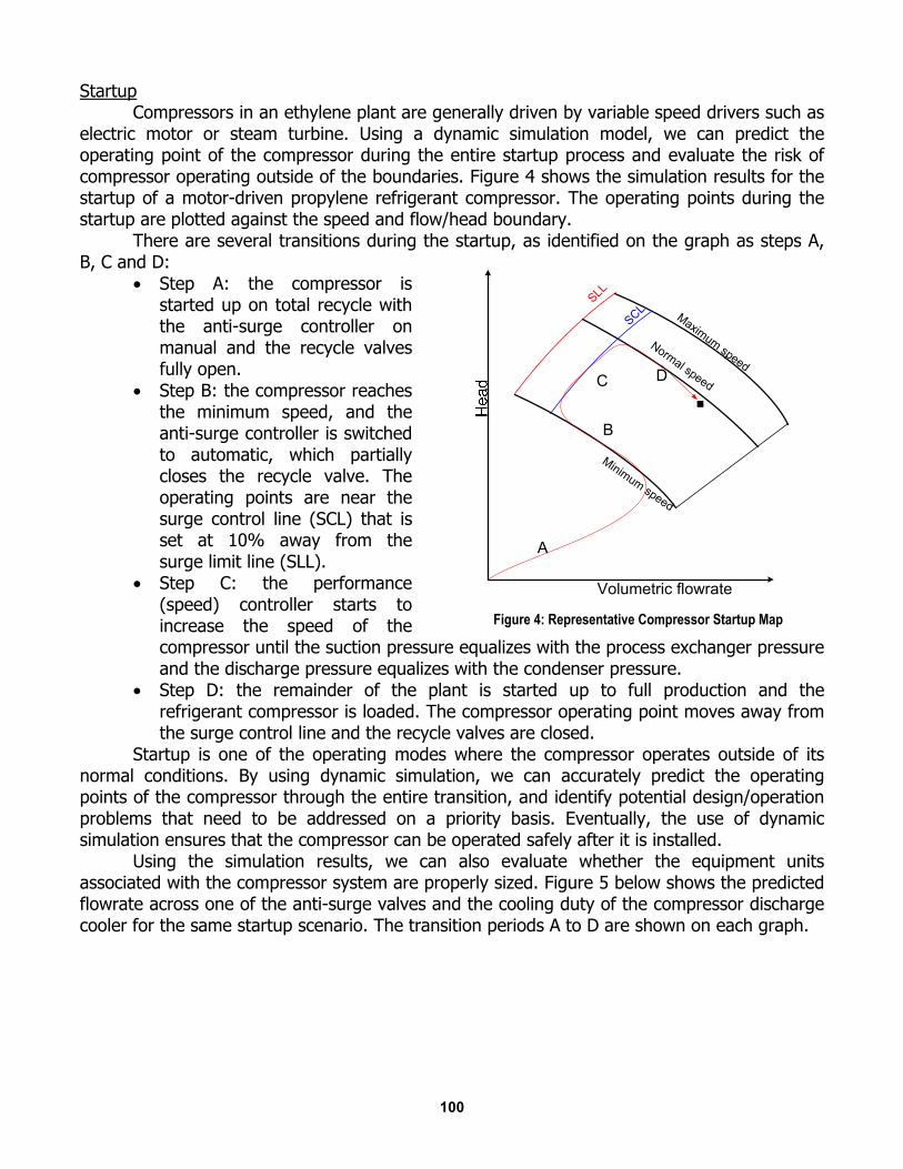
Startup Compressors in an ethylene plant are generally driven by variable speed drivers such as electric motor or steam turbine. Using a dynamic simulation model, we can predict the operating point of the compressor during the entire startup process and evaluate the risk of compressor operating outside of the boundaries. Figure 4 shows the simulation results for the startup of a motor-driven propylene refrigerant compressor. The operating points during the startup are plotted against the speed and flow/head boundary.

There are several transitions during the startup, as identified on the graph as steps A, B, C and D:

• Step A: the compressor is started up on total recycle with the anti-surge controller on manual and the recycle valves fully open.

• Step B: the compressor reaches the minimum speed, and the anti-surge controller is switched to automatic, which partially closes the recycle valve. The operating points are near the surge control line (SCL) that is set at 10% away from the surge limit line (SLL).

• Step C: the performance (speed) controller starts to increase the speed of the compressor until the suction pressure equalizes with the process exchanger pressure and the discharge pressure equalizes with the condenser pressure.

• Step D: the remainder of the plant is started up to full production and the refrigerant compressor is loaded. The compressor operating point moves away from the surge control line and the recycle valves are closed.

Startup is one of the operating modes where the compressor operates outside of its normal conditions. By using dynamic simulation, we can accurately predict the operating points of the compressor through the entire transition, and identify potential design/operation problems that need to be addressed on a priority basis. Eventually, the use of dynamic simulation ensures that the compressor can be operated safely after it is installed. Using the simulation results, we can also evaluate whether the equipment units associated with the compressor system are properly sized. Figure 5 below shows the predicted flowrate across one of the anti-surge valves and the cooling duty of the compressor discharge cooler for the same startup scenario. The transition periods A to D are shown on each graph.

SLL

Maximum speed

Minimum speed

Normal speed

Volumetric flowrate

A

SCL

B

C D

Figure 4: Representative Compressor Startup Map

100

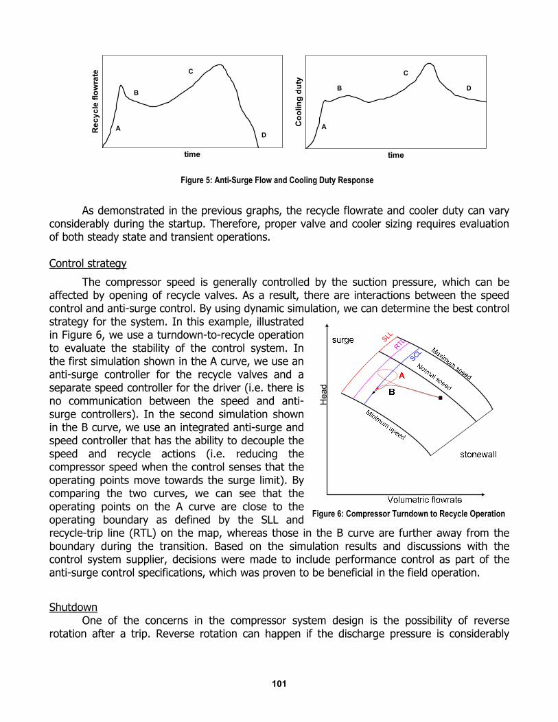
As demonstrated in the previous graphs, the recycle flowrate and cooler duty can vary considerably during the startup. Therefore, proper valve and cooler sizing requires evaluation of both steady state and transient operations. Control strategy

The compressor speed is generally controlled by the suction pressure, which can be affected by opening of recycle valves. As a result, there are interactions between the speed control and anti-surge control. By using dynamic simulation, we can determine the best control strategy for the system. In this example, illustrated in Figure 6, we use a turndown-to-recycle operation to evaluate the stability of the control system. In the first simulation shown in the A curve, we use an anti-surge controller for the recycle valves and a separate speed controller for the driver (i.e. there is no communication between the speed and anti-surge controllers). In the second simulation shown in the B curve, we use an integrated anti-surge and speed controller that has the ability to decouple the speed and recycle actions (i.e. reducing the compressor speed when the control senses that the operating points move towards the surge limit). By comparing the two curves, we can see that the operating points on the A curve are close to the operating boundary as defined by the SLL and recycle-trip line (RTL) on the map, whereas those in the B curve are further away from the boundary during the transition. Based on the simulation results and discussions with the control system supplier, decisions were made to include performance control as part of the anti-surge control specifications, which was proven to be beneficial in the field operation.

Shutdown

One of the concerns in the compressor system design is the possibility of reverse rotation after a trip. Reverse rotation can happen if the discharge pressure is considerably

Figure 5: Anti-Surge Flow and Cooling Duty Response

time

Rec

ycle

flow

rate

A

B

C

D

time

Coo

ling

duty

A

B

C

D

SLLH

ead

SCLRTL

Figure 6: Compressor Turndown to Recycle Operation

101

higher than the suction pressure at the moment the compressor stops (i.e. P2 is considerably greater than P1 as shown in Figure 7). The risk is high when there is a large discharge volume but the recycle valve is not adequate to depressure the discharge volume quickly during coastdown.

In a recent project, dynamic simulation was used to predict speed decay and the pressure differential across the compressor. The results are shown in Figure 8 below.

In this study, the results showed that when the compressor stopped, the pressure differential was small (less than 5 psi), so the risk of reverse rotation was low. To further reduce the risk, an isolation valve was added to the compressor discharge (circled in the sketch) with a control action to close the isolation valves on trip. Field operation confirmed the effectiveness of the design. It is worth noting that the results from this type of modeling are sensitive to the speed decay during coastdown. To ensure the validity of the results, the predicted coastdown curve should be reviewed by the compressor supplier or validated by field testing. Compressor Simulation Summary These examples show how dynamic simulation can be used to evaluate compressor operation and protection over a wide range of operating conditions and identify design and operation issues prior to commissioning. Industry experience shows that in many instances the use of rigorous dynamic simulations was able to identify and resolve design issues that could not be fully addressed by just steady state simulation (Ref 5, 6).

Rigorous Furnace Simulation Ethylene cracking furnaces are highly complex equipment. Efficient operation of furnaces requires a thorough understanding of the following issues:

a) pass-by-pass control of reactor outlet temperature and coking b) control of cracking in the radiant coils and transfer lines

Figure 8: Compressor Speed Decay and Discharge-Suction Pressure Differential during Coastdown time

Com

pres

sor s

peed

timePr

essu

res

Figure 7: Pressures Differential across a Compressor

102

c) accurate balancing of pre-heat needs with reaction duty needs Studying these issues requires a rigorous dynamic simulation model with the following components:

a) an accurate yield model that can predict the product distribution over a wide range of operating conditions. In this example, the yield model was compiled in Fortran and linked to the dynamic model as a .dll file.

b) calculation of pre-cracking in the cross-over c) accurate thermodynamics for the characterization of a wide variety of feedstock d) physical dimension of the furnace, including the coils, radiant tubes and fire box e) two-phase vaporization, heat transfer and pressure drop f) details of control scheme for feed, firing, coil outlet temperature (COT), excess

oxygen and ID fan The example below (Figure 9) shows a typical lineup of a naphtha or gas type of cracker. Typical scenarios that can be studied for such furnaces are transition from cracking to decoking and then back to cracking, change of firing conditions, change of hydrocarbon/steam ratio, trip of induced draft (ID) fan and pass-by-pass variations, such as excess coking in one pass or decoking in one pass.

Recently, dynamic simulation was used to evaluate the stability of different furnace control schemes. Figure 10 below shows the simulation results for one of simulation scenarios – increase of firing at time 0. As a result of firing change, the coil outlet temperature (COT) increases momentarily before the returning back to the set point after the control system

Figure 9: Gas or Naphtha Cracker Furnace Simplified Schematic

103

increases the feedrate. By using these kinds of results, we were able to confirm the stability of the overall control system and tune the controllers prior to commissioning.

Another application of a rigorous furnace model was to study “what-if” cases for basic design. All major components of the furnace were integrated into a single model: hydrocarbon/steam in the coils, fluegas in the stack, firing and cracking. This kind of integrated model can be used to quickly evaluate design alternatives such as changes in the heat transfer areas of convective bundles, impact of fuel type, impact of changes in various control set points, etc.

Steam System Simulation A simplified representative schematic of an ethylene plant steam system is shown in Figure 11 below for illustrative purposes. The four horizontal headers represent the low-pressure (at the bottom), medium-pressure, high-pressure and high-high-pressure steam headers. Ethylene plants are complex heat integrated systems where the energy from the process (shown in Figure 11 as coming from Plants 1 and 2) is used to generate high-pressure steam which is then used to power steam turbines, provide process heat to auxiliary systems, supply the ‘dilution’ steam used in the process, and in some cases directly used for online ‘decoking’ of furnace tubes. The systems are further complicated by having multiple pressure levels and auxiliary backup boilers in case of plant trips, all of which leads to complex control system design for the steam letdown stations, the handling of process upsets or trips, and sparing philosophies.

Figure 10: Representative Simulation Results for Furnace COT Control

time

Coi

l out

let t

empe

ratu

re

time

Feed

rate

104

The list of issues that lead to complexities in ethylene plant steam system design can be summarized as follows:

• Multiple sources of steam – e.g. primary steam generated through heat recovery from process and auxiliary boilers

• Large let down valves to provide emergency steam to lower pressure headers • Large multi-stage turbines with extraction and admission steam • Minimum pressure limits in each of the steam headers • Very compact design with relatively small header volumes • Steam and motor drives

Thus dynamic simulation has been frequently used in the industry to study the following:

• Confirm adequacy of auxiliary boiler ramp up specifications • Confirm optimum base loading for auxiliary boilers • Confirm stability of the steam headers and control system with respect to critical

process variations and upsets • Confirm adequacy of let-down valve sizing and controls • Verify relief valve placement and size

Figure 11: Representative Steam System

105

• Determine preliminary tuning constants for control loops In cases where a single integrated steam system services multiple plants in a complex, advanced feedforward controls and de-coupling strategies may also need to be designed and tested. The plots in Figure 12 below show examples of the complex dynamics that might result in steam systems due to plant upsets and trips. The first figure shows the variation of steam make from Heat Recovery Steam Generator (HRSG) due to a gas turbine trip, while the second figure shows the ramp up dynamics of an auxiliary boiler due to process trip. As the results show in the cases below, the control systems were able to manage the upset however it is the quality of control that is the key criteria for design based on these dynamic results.

The benefits generated from such studies can be summarized as: a) prevention of under-sizing or over-sizing of let down and relief valves, b) validation of the sizing and ramping specifications for auxiliary boilers, c) validation of basic control philosophy and tuning constants prior to actual plant startup, and d) validation of alarm settings and trip points for the overall system. The last benefit is critical in cases where steam system upsets may lead to process trips caused by inadequate setting of process trip points.

Fuel Gas System Simulation Fuel gas systems are another critical area where dynamic simulation is often used to determine the adequacy of the system with respect to plant upsets and trips. An illustrative sketch of a representative fuel gas system is shown in Figure 13 to highlight the practical complexities of such a system. Note the potential multiplicities of fuel types, different user levels, and the various backup and failover strategies. Typically the Low Pressure (LP) users are process boilers, incinerators and such. In this example, the plant also has gas turbines that operate with High Pressure (HP) fuel gas. The requirement is to maintain header pressures and fuel gas quality parameters such as Heating Value and Wobbe Index. There may also be restrictions on rate of change of these fuel gas parameters. Dynamic simulation of postulated plant upsets is then the only useful way to validate the adequacy of the process and control system design for the fuel systems.

Figure 12: Representative Steam System Dynamics due to Process Upsets

timeH

eade

r pre

ssur

e

Con

trolle

r out

put

Header pressure

Controller output(output of auxiliary boiler)

time

Stea

m g

ener

atio

n ra

te

106

Figure 14 below shows some typical examples of dynamic responses for fuel gas systems. The first plot shows the pressure recovery and heating value response to a primary fuel source trip. As the plot shows, pressure recovery (top curve on the first graph) is possible in a few minutes; however the header may experience a low pressure trip in addition to a decrease in heating value. The second plot shows the ramp up rate of the secondary fuel sources following a trip.

Decisions regarding the size of the equipment or specific control strategies that have to be designed for a specific plant can be derived or validated based on these kinds of responses.

Figure 14: Representative Fuel Gas System Dynamics due to Process Upsets

05

101520253035404550

time

Fuel

rate

Primary fuel gas

Makeup fuel from feed

Makeup fuel from LPG

time

Hea

der p

ress

ure

Hea

ting

valu

e

Header pressure

Heating value

Figure 13: Representative Fuel Gas System

Main Fuel Gas Supply

Aux. Fuel Gas

Fuel User 1

LPG

Steam

Condensate

Vaporizer

Aux.LPG

TIC001

PIC001

FIC003 FIC

002

FIC001

Aux. Fuel Gas

Fuel User 2

Fuel User 3

Fuel User 4

LIC001

LP User 1

LP User 2

LP User 3

LP User 4

LP HDR

HP HDR

PIC002

107

In this example, the size of the LPG makeup capacity was increased to minimize the fluctuations in the fuel gas system on the loss of primary fuel gas.

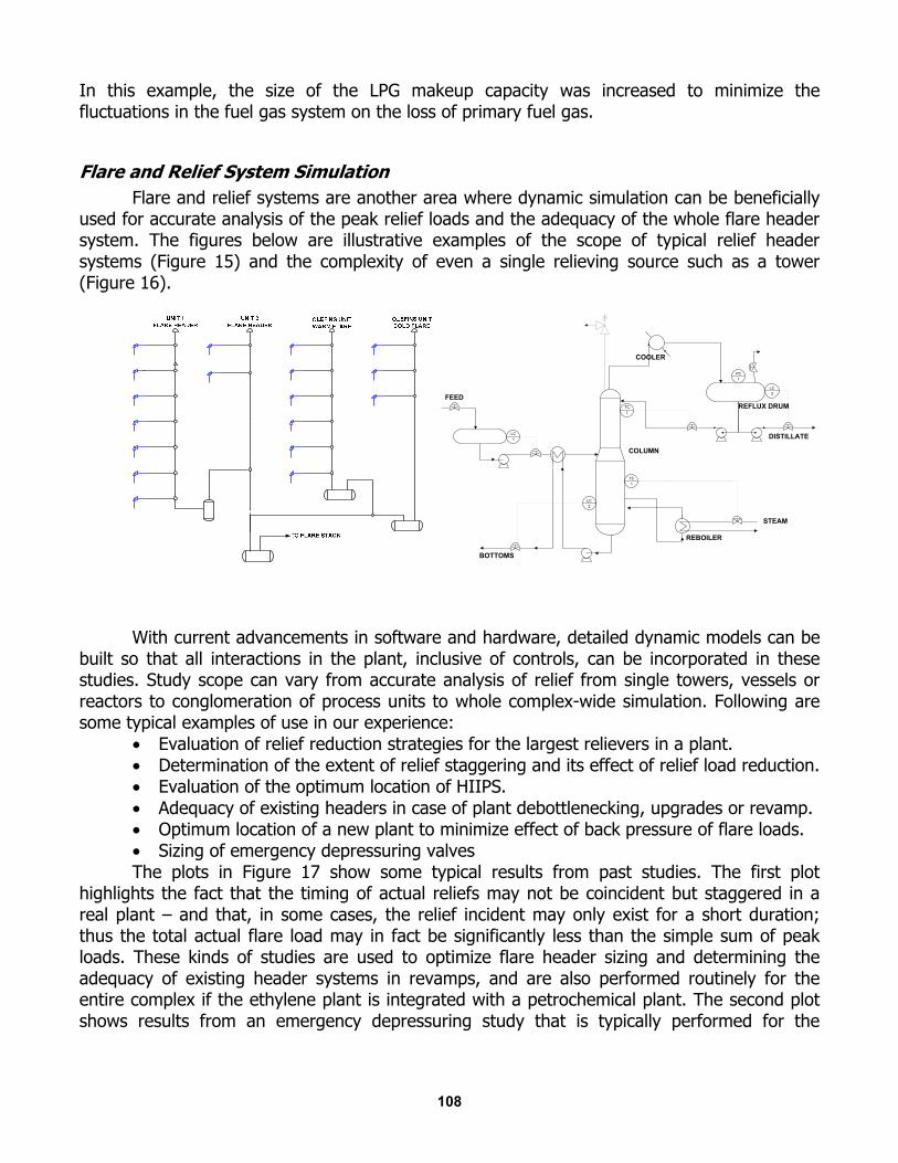
Flare and Relief System Simulation Flare and relief systems are another area where dynamic simulation can be beneficially used for accurate analysis of the peak relief loads and the adequacy of the whole flare header system. The figures below are illustrative examples of the scope of typical relief header systems (Figure 15) and the complexity of even a single relieving source such as a tower (Figure 16).

With current advancements in software and hardware, detailed dynamic models can be built so that all interactions in the plant, inclusive of controls, can be incorporated in these studies. Study scope can vary from accurate analysis of relief from single towers, vessels or reactors to conglomeration of process units to whole complex-wide simulation. Following are some typical examples of use in our experience:

• Evaluation of relief reduction strategies for the largest relievers in a plant. • Determination of the extent of relief staggering and its effect of relief load reduction. • Evaluation of the optimum location of HIIPS. • Adequacy of existing headers in case of plant debottlenecking, upgrades or revamp. • Optimum location of a new plant to minimize effect of back pressure of flare loads. • Sizing of emergency depressuring valves

The plots in Figure 17 show some typical results from past studies. The first plot highlights the fact that the timing of actual reliefs may not be coincident but staggered in a real plant – and that, in some cases, the relief incident may only exist for a short duration; thus the total actual flare load may in fact be significantly less than the simple sum of peak loads. These kinds of studies are used to optimize flare header sizing and determining the adequacy of existing header systems in revamps, and are also performed routinely for the entire complex if the ethylene plant is integrated with a petrochemical plant. The second plot shows results from an emergency depressuring study that is typically performed for the

LC2

PC1

LC3

TC1

TC1

COLUMN

REFLUX DRUM

DISTILLATELC1

BOTTOMS

FEED

STEAM

REBOILER

COOLER

108

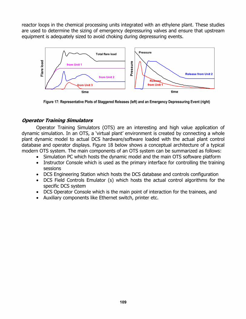
reactor loops in the chemical processing units integrated with an ethylene plant. These studies are used to determine the sizing of emergency depressuring valves and ensure that upstream equipment is adequately sized to avoid choking during depressuring events.

Operator Training Simulators Operator Training Simulators (OTS) are an interesting and high value application of dynamic simulation. In an OTS, a ‘virtual plant’ environment is created by connecting a whole plant dynamic model to actual DCS hardware/software loaded with the actual plant control database and operator displays. Figure 18 below shows a conceptual architecture of a typical modern OTS system. The main components of an OTS system can be summarized as follows:

• Simulation PC which hosts the dynamic model and the main OTS software platform • Instructor Console which is used as the primary interface for controlling the training

sessions • DCS Engineering Station which hosts the DCS database and controls configuration • DCS Field Controls Emulator (s) which hosts the actual control algorithms for the

specific DCS system • DCS Operator Console which is the main point of interaction for the trainees, and • Auxiliary components like Ethernet switch, printer etc.

Figure 17: Representative Plots of Staggered Releases (left) and an Emergency Depressuring Event (right)

time

Pres

sure

Pressure

Releasefrom Unit 1

Release from Unit 2

time

Flar

e lo

ad

Total flare load

from Unit 3

from Unit 1

from Unit 2

109

The following are some of the key functionalities of OTS systems:

• Ability to initialize the system from any initial state such as normal design or cold start – this allows many modes of training

• Ability to save and restore any intermediate operating state – this allows training to occur over long durations without losing data and also to capture interesting case studies for future review

• Ability to cause standard or generic equipment faults – this allows the operators to train on wide variety of faults and upsets

• Ability to run pre-programmed scenarios – this allows operators to repeatedly train on specific scenarios to gradually build up expertise

• Ability to track operator performance – this provides Instructors with an objective measure of operator proficiency both as a way to gauge skills progress and as a method for operator certification for specific job classifications.

The primary uses of these systems can be summarized as follows: • comprehensive training of plant operators – while these systems are primarily used

for new operator training, they are also used for refresher training and for operator certification

• validation and optimization of plant operating procedures, and • control system refinement.

Figure 19 below shows a representative example of an OTS display for an ethylene furnace to illustrate the degree of detail and rigor that is typically included. In general the

Figure 18: Typical Architecture of an Operator Training Simulator

110

models consist of a whole plant dynamic model inclusive of all basic controls, all field operations, all panel operations and relevant safety logic.

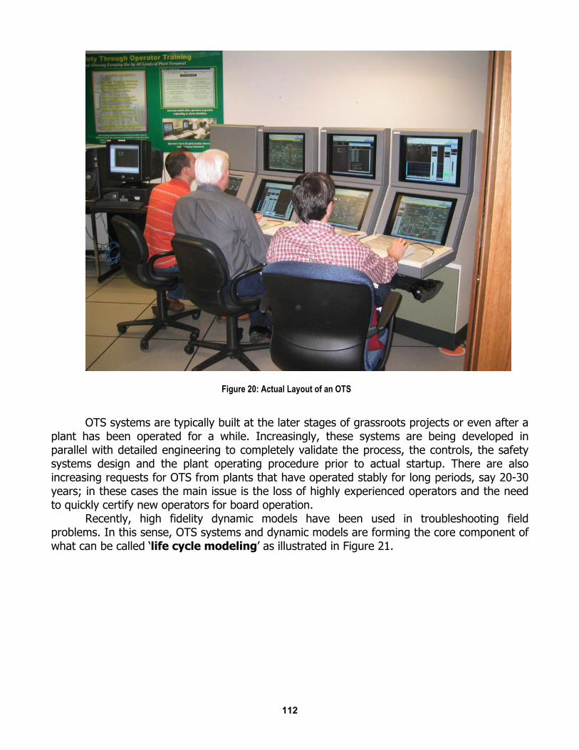
Figure 20 below shows the layout of a complete OTS system. The computer on the left is one of the PC’s for the Simulation Components. The three sets of screens on the right are the Operator Consoles.

Figure 19: Typical Furnace Detail Display in an OTS

111

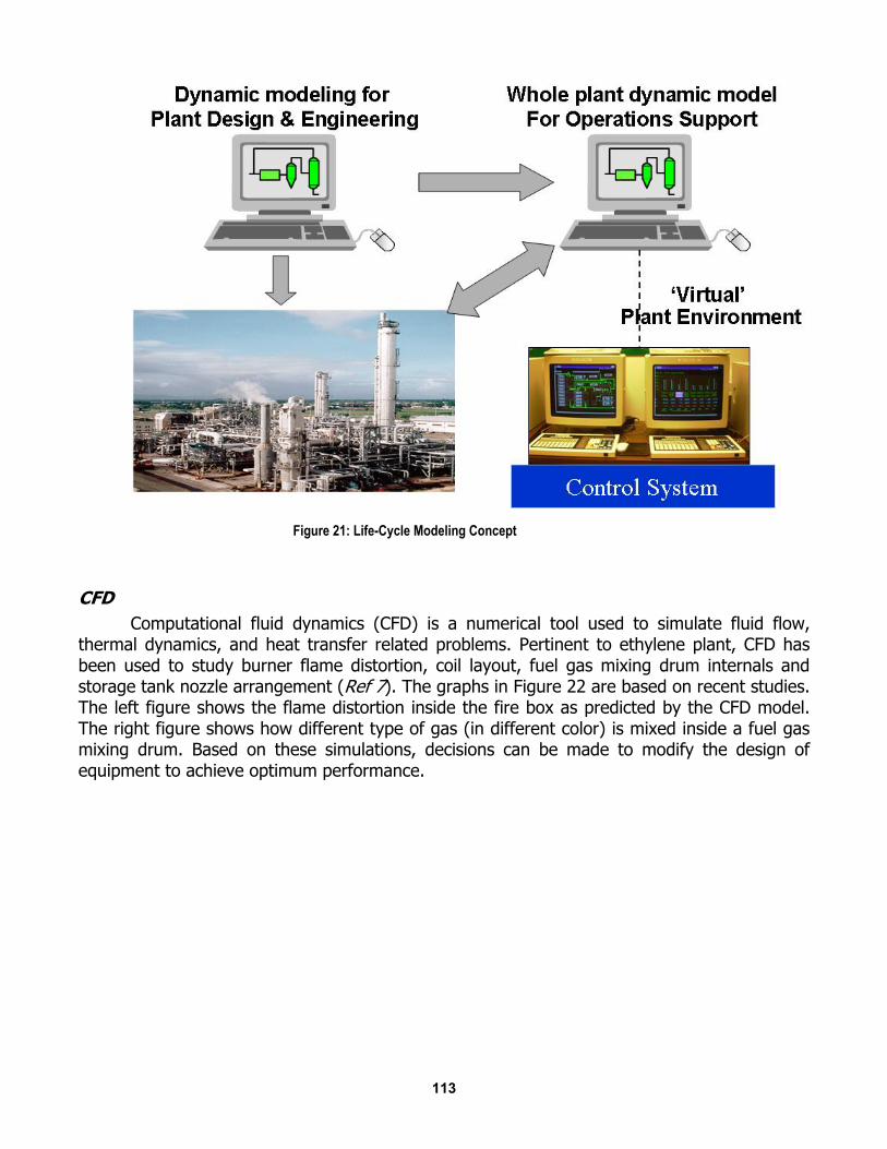
OTS systems are typically built at the later stages of grassroots projects or even after a plant has been operated for a while. Increasingly, these systems are being developed in parallel with detailed engineering to completely validate the process, the controls, the safety systems design and the plant operating procedure prior to actual startup. There are also increasing requests for OTS from plants that have operated stably for long periods, say 20-30 years; in these cases the main issue is the loss of highly experienced operators and the need to quickly certify new operators for board operation. Recently, high fidelity dynamic models have been used in troubleshooting field problems. In this sense, OTS systems and dynamic models are forming the core component of what can be called ‘life cycle modeling’ as illustrated in Figure 21.

Figure 20: Actual Layout of an OTS

112

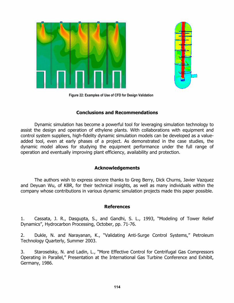
CFD Computational fluid dynamics (CFD) is a numerical tool used to simulate fluid flow, thermal dynamics, and heat transfer related problems. Pertinent to ethylene plant, CFD has been used to study burner flame distortion, coil layout, fuel gas mixing drum internals and storage tank nozzle arrangement (Ref 7). The graphs in Figure 22 are based on recent studies. The left figure shows the flame distortion inside the fire box as predicted by the CFD model. The right figure shows how different type of gas (in different color) is mixed inside a fuel gas mixing drum. Based on these simulations, decisions can be made to modify the design of equipment to achieve optimum performance.

Figure 21: Life-Cycle Modeling Concept

113

Conclusions and Recommendations Dynamic simulation has become a powerful tool for leveraging simulation technology to assist the design and operation of ethylene plants. With collaborations with equipment and control system suppliers, high-fidelity dynamic simulation models can be developed as a value-added tool, even at early phases of a project. As demonstrated in the case studies, the dynamic model allows for studying the equipment performance under the full range of operation and eventually improving plant efficiency, availability and protection.

Acknowledgements The authors wish to express sincere thanks to Greg Berry, Dick Churns, Javier Vazquez and Deyuan Wu, of KBR, for their technical insights, as well as many individuals within the company whose contributions in various dynamic simulation projects made this paper possible.

References 1. Cassata, J. R., Dasgupta, S., and Gandhi, S. L., 1993, “Modeling of Tower Relief Dynamics”, Hydrocarbon Processing, October, pp. 71-76. 2. Dukle, N. and Narayanan, K., “Validating Anti-Surge Control Systems,” Petroleum Technology Quarterly, Summer 2003. 3. Staroselsky, N. and Ladin, L., “More Effective Control for Centrifugal Gas Compressors Operating in Parallel,” Presentation at the International Gas Turbine Conference and Exhibit, Germany, 1986.

Figure 22: Examples of Use of CFD for Design Validation

114

4. Wilson, J. and Sheldon, A., 2006, “Matching Antisurge Control Valve Performance with Integrated Turbomachinery Control System,” Hydrocarbon Processing, August, pp. 55-58. 5. Patel, V., Feng, J., Dasgupta, S., Ramdoss, P., and Wu, J., 2007, “Application of Dynamic Simulation in the Design, Operation and Troubleshooting of Compressor Systems,” Presented at the 13th Turbomachinery Symposium. 6. Wu, J., Feng, J., Dasgupta, S., and Keith, I., 2007, “A realistic dynamic modeling approach to support LNG Plant Compressor Operation,” LNG Journal, October, pp. 27-30. 7. Barnett, D. and Deyuan, W., "Fluegas Circulation and Heat Distribution in Large Scale Down-fired Reformer Furnaces,” Presentation at the AIChE, September 2000.

115