US Crashes of 2008 and 1929How did the French market react? An empirical

study.

Raphaël Hekimian∗ David Le Bris†

April 24, 2015

Abstract

We compare the reaction of the Paris bourse to the US crashes during boththe 2008 and the 1929 crises. We constitute a new dataset of daily French stockprices from February 1929 to March 1930 that we combine to the already ex-isting daily series of the Dow Jones. We also use newspapers and minutes fromthe Banque de France and from the Paris Stock Exchange’s brokers syndicatein order to confront quantitative data with historical narratives. We finallyrun contagion tests in both periods, using adjusted correlation coefficients totest for pure contagion. In 1929, the Paris stock market does not exhibit anyreaction to the New-York crash. The recent crisis is totally different with aclear contagion of the US crash. This study highlights a significant differencebetween the two crises and provides strong evidence that the transmission ofthe Great Depression used other channels than stock markets.

JEL Classification: G150, G010, N12, N13Key Words: Financial history, Financial crisis, Stock market, Contagion

∗EconomiX-CNRS, UPOND, 200, avenue de la République, 92001 Nanterre, France. Email:raphael.hekimian@yahoo.fr

†Kedge Business School, 690, Cours de la Libération, 33405 Talence. Email:david.lebris@gmail.com

1

1 Introduction

World has been affected by an economic and a financial crisis started in 2008 in theUS. Stock markets all over the world followed New-York in his fall. Most of theeconomists quite agree that the only comparable crisis is the Great depression of the1930s (Almunia and al., 2010). This major event of the 20th century also startedin the US before spreading all over the planet. France is one of the most impactedcountries by the Great Depression even if it is with a lag compared to the US; theFrench industrial production of 1937 is 28 % lower than the one observed in 1929(Landes, 2000 p. 534).

The US stock market crash is usually seen as the starting point of the Great De-pression. But the channel of the propagation of the crisis from US to the other partsof the world especially to France is still an open question. A propagation of the UScrash in France could have happened in 1929 because the two markets were relatedwithout capital controls. The US crash Paris could have had an important echo inFrance since the Paris market was seen in the early thirties as the most importantfinancial place of continental Europe (Jacques, 1932). Studying the internationalcorrelations among the major world equity markets over 150 years, Goetzmann andal (2001) show that the equity market correlation between Paris and New York dur-ing the interwar was at the his second highest history just after the recent period.The period we study in our empirical exercise stops in 1930, when controls on capitalflows were not that important, allowing large international flows (see Obstfeld andTaylor 1997 and Mitchener and Wandschneider 2014). In fact, the main controls tocapital flows appeared by 1931 and afterward, when the UK went out of the goldblock and imposed controls on foreign exchanges.

The literature generally mentions that “the Great Depression was transmittedinternationally through trade flows, capital flows and commodity prices.” (Almuniaand al., 2010). Especially for France, the devaluation of the Sterling in September1931 is frequently observed as the starting point of the local version of the Great De-pression (Sauvy, 1984). Thus, even implicitly, most of the existing literature excludesthe stock market as a channel of transmission but without dedicated demonstration.This lack has become more problematic since the crisis of 2008 exhibits a very strongcorrelation among international stock markets.

In this paper, we investigate the short term reaction of the Paris Bourse in thesix month after both the US crashes of October 1929 and Lehman failure in 2008.To measure the behavior of the French market in 1929 we build a new dataset ofdaily stock prices collected at the archives of the French bourse (conserved at theFrench Ministry of Finance). These daily prices provide a clear demonstration thatthe propagation of the Great Depression is not the result of a contagion of the stockmarket crash. Indeed, the French stock market remains stable during the US crash.This stability is demonstrated using four kinds of evidence: a descriptive measureof the stability of the French market during the US crash, the lack of any structuralbreaks in the French series in 1929, the stability of the volumes trades in Paris and

2

few narratives of the practitioners of that time.

Thus, we lend support to the standard claim of channels different than stockmarket by providing strong evidences of the absence of any contagion (co-movementof asset prices beyond what is warranted by fundamentals) in 1929. To our bestknowledge, it is the first study aiming at proving the absence of any contagion ofthe Wall Street crash to Europe, using data on a daily basis.

A second contribution is to characterize the relationship between the French andUS markets using these high frequency data and compare it with the same indices inthe recent period. There is no doubt that the US stock market leads the French onein the recent period but it is less clear in 1929. Despite the leading role of the USeconomy at that time, the two markets remain broadly independent. We do observean influence of the US market on the French one but at a weak level as demonstratedby the very low correlation among the two markets.

Previous studies indicate important differences in the behavior of the two mar-kets. The US market exhibits a very high volatility during the Great Depressioncontrasting to a stable level for the rest of the history (Schwert, 1997). In France,the maximum of the volatility is ten years later at the end of the World War II (LeBris, 2012). Using our daily dataset, we investigate more deeply these differencesand confirm the higher stability of the French market compared to the US in 1929.This stability is not affected by the US crash.

Our evidence joins claims made by Mauro and al. (2002 and 2006) in which theyargue that the modern global financial system suffers from contagion whereas thehistorical financial system of the pre-world War I era was less prone to it. We showthat it is still true during the interwar period, at least between US and France. Theabsence of contagion is consistent with the structural differences between the twomarkets.

The last contribution of this research is to identify a crucial difference betweenthe episodes of 2008 and 1929. The behavior of the French market in 1929 contrastsstrongly with what has been observed during the recent crisis with a general dropon international stock market after the Lehman default. On this crucial point, 2008is thus different from 1929. Several studies offer narrative comparisons between theGreat Depression and the Great Recession, as the recent crisis is sometimes named.They stressed the similarities between the two episodes. For example, Peicuti (2014)makes an interesting list of their analogies, highlighting some stylized facts to showthe similarities between the periods 1921-1929 and 2001-2007. In particular, therapid growth without contraction, the increase in global liquidity and the lack ofinflation are common to both France and the US for those periods. Moreover, theinternational spillover effects are a strong common feature of both crises. Gross-man and Meissner (2010) also compare the two international crises and try to drawlessons from them in terms of both trade and financial linkages, but without empir-ical tests. In the recent empirical literature, Mehl (2013) study the impact of global

3

volatility shocks from 1885 to 2011 with monthly data. One of his results is thatthe two most severe global stock market volatility shocks are the late October 1929stock market crash at the NYSE and the collapse of Lehman Brothers in 2008.

After describing the dataset in Section 2, Section 3 presents four types of ev-idences demonstrating the absence of any specific movement in the French stockmarket in 1929. Section 4 shows a clear contagion in 2008 but not in 1929. We testfor the presence of contagion after the crash at the NYSE in both 1929 and 2008.In section 5, we implement VAR / VECM models in order to characterize the rela-tionship between the French and the American stock price indexes. In both periods,the returns on the American index seem to have an influence over the French one.Section 6 concludes.

2 Data

Regarding French stock prices during the interwar period, only monthly data areavailable. The two most common sources are the stock price index of the Leagueof Nations and the one of the Statistique Générale de la France (i.e. the NationalInstitute for Statistics). Both of those indexes are un-weighted. More recently, LeBris and Hautcoeur (2010) constructed a Blue Chips index of French stock pricesweighted by market capitalization over 150 years, but the frequency is also monthly.

To build the French market daily prices of 1929, we collected daily spot1 pricesfor forty individual stocks listed at the official list2 of the Paris Bourse. Those stocksare the forty highest market capitalizations at the beginning of 1929 as identified byLe Bris and Hautcoeur (2010). Our dataset covers the period from February 1929through the end of March 1930.

We reconstruct a blue chip weighted index we call HCAC 40 (H for Historical),for which the daily return is given by:

RHCACt =

∑40i=0 number of sharei × price of shareit+1∑40i=0 number of sharei × price of shareit

− 1

For each stock,3 we collected the closing price every day. If a stock has no trans-action price for a given day, we use the last transaction price in order not to keepthe index away from fluctuations due to a lack of liquidity, and not due to a themechanism of supply and demand.

This index allows us to interpret most of the movements of the French equitymarket since we know that the aggregated market capitalization of our forty firms

1The Paris Stock Exchange had already a term market and an option market but we onlycollected prices for the spot market.

2There was already an OTC market inside the Paris Bourse, but all the data we collected onlyconcerns the official market.

3The complete list of stocks we used are reported in Appendix 1.

4

represents around 60% of the total market capitalization of the Paris Bourse at thistime (Le Bris and Hautcoeur, 2010). A blue chips index does reflect the overallmarket (Annaert and al., 2011). The daily data of 2008 are from Euronext CAC 40.We checked whether our index could be biased since some companies might be moreprone to international fluctuations than others. Typically, the banking sector couldsuffer more from exogenous shocks like the Great Crash of October 1929, while com-panies which have their business totally grounded in France (e.g. railroads) shouldbe more isolated. For that matter, we made a sectorial analysis (reported in ap-pendix 1) where we computed a banking index, that include all of the nine banks wehave in our database, and a “French only” index that include railroads, utilities andcoal mines firms. The Figure 8 presented in Appendix 1 shows that the trends seemto be similar between the two sub-indices and the main one. This claim is verifiedthrough a simple test on the means and the variances of the indice returns.4

For US data, we use the Dow Jones Industrial index. While the Dow Jones is aninaccurate index for measuring long-term stock performances, since it is weighted bystock prices, it can be useful in the analysis of short term movements. Additionally,it is the single source of daily data for the 1929 period. We also take the Dow Jonesfor the recent period in order to have the same measure in both periods.5

3 1929 in the French stock market: a peaceful pe-riod

We rely on four types of evidences to demonstrate that the French stock market isnot affected by any specific phenomenon in 1929.

3.1 Descriptive analysis

It is well-known that the French market, like other international markets, closely fol-lowed the US into the crash after the failure of Lehman brothers (Figure 1). Despitefew differences in the behaviours of the two markets prior months, we graphicallyidentify that the two markets evolve closely after the Lehman failure.

The story is really different when we look at the 1929 case (Figure 2) since noshock occurred on the French stock market after the crash at the NYSE. It is quitesurprising to observe that even the worst days in the NYSE seems free of any impactin the Paris market; 1929 October 28, the Dow Jones fell by 13.47% but our Frenchindex decreased by 0.60% and 2.99% the day after when the Dow Jones sufferedanother fall of 11.73%. After these two days, the loss is 23% in New-York and only5% in Paris. The only sharp decrease that we can observe is in late November (reddashed circle), so over a month after the crash. This absence of any contagion of theUS crash is really different from what was observed during the last financial crisis.

4Results are reported in Table ??, in Appendix 1.5We checked if the results would be different by taking the S&P 500, but the correlations

between this later and the Dow Jones is over 0.99 for the period.

5

Figure 1: Dow Jones and CAC Indices in 2008

Notes: base 2008M09=100.Source: Dow-Jones, Federal Reserve of Saint Louis; CAC, calculation from authors

In Appendix 2 are reported the graphs of the returns on the indexes in bothperiods. We easily observe that the magnitude of the volatility of the French indexin 1929 is a lot lower than the American one. It is quite different in 2008, wherethe magnitude of the volatility is very high for both indexes. Moreover, we can seevolatility clusters in each graphs but the French index in 1929: the Historical CAC40 does not exhibit any particular volatility structure, whereas modern financialseries are featured by asymmetric volatility.

3.2 1929 in France does not exhibit any structural break

A more formalized test for the presence of a specific activity in 1929 in France isto compare the stability of the parameters when we model the stock returns. Asin modern series, unit root tests6 (not reported) lead us to use returns, rather thanthe series in level to get stationary series. A first glance at the data indicate thatthe volatility of the returns does not seem to have a particular structure: the highvolatilities are not clearly followed by other high volatilities and it is the same forlow volatilities. It seems then legitimate to use linear specifications.

We use the Box and Jenkins (1970) methodology in order to specify the bestARMA process to model RCACt . We end up estimating an autoregressive process atthe order 1 (AR(1)):

RCACt = α0 + β1RCACt−1 + εt (1)

6ADF and Perron tests have been used to detect the trend for both series. Results show thatthey are all I(1).

6

Figure 2: Dow Jones and CAC Indices in 1929

Notes: base 1929M09=100.Source: Dow-Jones, Federal Reserve of Saint Louis; CAC, calculation from authors

Variables Coefficient Std. Error t-statistic p-valueα0 -0.0005 0.0006 -0.8051 0.42β1 -0.2299 0.0555 -4.1394 0.00***

Notes: ∗ ∗ ∗ denotes significance at the 1% confidence level.

Table 1: Results

The estimation output shows that the estimated βt is significant. Moreover, aftertesting for the absence of autocorrelation and homoscedasticity7 on the residuals,we find that εt follow a white noise. It is important to notice that we do not detectany ARCH effect, which is usually the case for equity returns (especially at a dailyfrequency).This feature allows us to test for the stability of the parameters. Indeed,since there are no issues on the residuals, we are able to apply a basic Chow testby estimating the model (1) in two sub-samples, before and after the crash at theNYSE in late October 1929.

F -statistic Log likelihood ratio Wald Statistics2.63 5.29 5.26(0.073) (0.071) (0.072)

Notes: Sample: 2/05/1929 - 2/31/1930. p-values are reported in parentheses.

Table 2: Chow Breakpoint Test: 10/28/1929

The p-value of the F -test (2,296) = 0.0736 > 0.05: the null hypothesis is rejectedat the 5% confidence level. The parameters are stable before and after the crash.

7We used a Ljung-Box test based on the correlogram of the residuals to detect the presence ofautocorrelation and an ARCH test for the homoscedasticity.

7

The crash in New-York is free of any effect on the nature of the stock price variationsin Paris.

3.3 The volumes traded in the Paris bourse remain stable

A third evidence of the absence of any specific phenomenon in France in 1929 is thestability of the volumes exchanged. The increase of the quantity of stocks traded inNYSE during the crash is a common knowledge. Even in the absence of a violentprice movement in France the US crash could have had consequences in the Frenchmarket through specific movements leading to a rise of the volumes traded.

When researchers in history of finance study the Paris Bourse, a prominent weak-ness is the lack of data about the volume traded. We tried to solve this issue bycollecting two series that we take as proxies for the volumes: the tax on financialtransactions and the amount of compensations in between the brokers. However,both series have several limits that we discuss below.

The first one is a tax on financial transactions which is available on bi-monthlybasis. The tax levies a fixed rate on the total volume traded at the Paris Bourse forsecurities listed on the official list, for both the spot and the term markets. Sincewe only have spot prices, there is an upward bias that is difficult to estimate if wewant to link our prices with this volume proxy. We can suppose this bias constantovertime. Moreover, there is a frequency issue because our stock prices are dailyand the tax is only available every two weeks. Figure 3 exhibits this series:

Figure 3: Bi-monthly amount of taxes raised in million Francs

Source: Authors.

Our second proxy for the volume traded is the daily amount of compensationsbetween brokers operating on the official market. Here, the frequency is daily andmoreover, it only concerns the spot market. Nevertheless, there is another potentialbias, once again very hard to estimate. When a broker executes an order for a client,another broker has to compensate for the amount of the transaction, by an order

8

of his own clients that goes on the opposite way. But if a broker has already twoclients giving him opposite orders, he can compensate by himself and then doesn’thave to ask a colleague. In this case, the compensation is not reported in the brokerscompany’s balance sheet.8 This also constitutes a downward bias but we can alsosuppose it constant over time. Figure 4 illustrates this series:

Figure 4: Daily compensation in million Francs

Notes: Source: Authors.

We can see that the volumes are pretty stable except for the end of the year 1929where some pics appear in November and December, so few weeks after the crashat the NYSE. This seems to indicate some sort of lagged impact on the Paris StockExchange, but it contrasts with our descriptive data on prices.

3.4 Narratives of practitioners

In this subsection, we look in financial newspapers and in the archives of both theminutes of the Banque de France, and the Compagnie des agents de change. We alsolooked at some research papers published by French economists at the time. Theaim is to check if the story told by the contemporaries fits with our three quantita-tive evidences previously exposed.

Jean Dessirier (1930), a famous French analyst of the stock exchange, noticedthat French asset prices did not follow the downturn of US equity prices. He insistson the French monetary situation, featured by “the maintenance of an easy mone-tary situation, despite the international tension”. He tries to explain that the Frenchstock market hung on because of the nature of French investors comparing to theAmerican ones, much more prone to speculation.

8Until 1987, a brokers company called Compagnie des Agents de Change had the monopolyon all the transactions at the Paris Bourse, but the institution had to remain accountable by theState.

9

The French monetary situation of the late 1920’s and the early 1930’s has beenmuch studied in the literature about the Great Depression and it links with theGold Standard.9 This situation is featured by an increasing amount of gold reservesduring the period 1927-1932, while the authorities kept the monetary base stable byincreasing the cover ratio.We looked at the bi-weekly reports of the board of gover-nors of the Banque de France over the period and found some interesting statements.Indeed, Emile Moreau explicitly warns off against the monetary circulation move-ments in early 193010 and especially in terms of gold inflows coming from abroad. InMay 1930, he even plans on decreasing the discount rate after the Bank of Englanddecreased its own, in order not to see more gold inflowing. This suggests that thevery first goal of the authorities at this time was to keep the prices stable.

We also looked at the bi-monthly minutes of the Compagnie des Agents deChange. The only time they mentioned a bear market is on December the 5th.However, they do not explain the reasons of this downturn. They only focus on theannouncement made by the new government that the fiscal surplus will be investedin the economy and therefore that there are no reasons to be pessimistic.

Finally, we went through financial newspapers in order to find some citationsthat would explain the pics observable on Figure 4, as well as the decrease in theprices depicted on Figure 2 (dashed circle). We can read in Le temps of Novemberthe 18th that “rumours on failures in Germany did participate, to a certain extent,in the fall of the prices” and that “Before going back to business, the Paris’ Bourseis waiting to know the evolution of Wall Street”. These quotes suggest that whathappens in other financial places seems to influence the behaviour of investors inParis at that time. However, and more interestingly, the editions of November 21st,22nd, 26th and 27th all present the same explanation for the slump of late November:a wave of sale orders coming from foreign accounts, ‘in particular from Germany andEastern European countries”. However, they point out that those sales are quite wellabsorbed by French investors, which is confirmed by our data because the prices donot fall very sharply and for a short period. Finally, on December the 3st (the secondpic on 4), this day is a “liquidation day” (i.e. the day when every term and optioncontracts are either reported or concluded), which explains partially the increase inthe volume. However, it is also mentioned that the monetary situation is playinga large part in the good behaviour of the stock exchange: “The widecomfort of themonetary situation appears, regarding the stock market,at the same time than theexcellent position of the stock exchange”.

The study of those historical sources seems to confirm the descriptive analysis ofour data. In the next section, we make of comparison of the econometrical findingsof the study of the relationship between the returns on the Dow Jones the ones ofthe CAC 40 in both periods.

9 We can cite, among others, Hamilton (1987), Bernanke and James (1991), Eichengreen andTemin (1996), Irwin (2012).

10See bi-weekly minutes of the Banque de France from 1930/01/02; 1930/01/23; 1930/01/30;1930/02/20; 1930/03/20.

10

4 The presence of contagion in 2008 but not in 1929

Since we didn’t detect any specific movement in the French stock market in 1929, weshould reject a contagion from New-York to Paris. Based on the Forbes and Rigobon(2000, 2002) methodology, we adjust correlation coefficients from the heteroscedas-ticity bias that occurs during crisis periods. Indeed, volatility increases after shockson stock markets and the two authors show that the usual correlation coefficientsare then biased by construction.

Such a methodology has been used in Bordo and Murshid (2000) to test forcontagion for several historical international financial crises, including the interwarperiod. However, they use weekly foreign government bond prices traded at theNYSE for several countries, while we focus on only two countries and use stockprices traded in each country’s stock exchange.

For our two series of stock index returns RDJt and RCACt , the Pearson correlationcoefficient is given by:

ρRDJt ,RCACt=

Cov(RDJt , RCACt)

σRDJt× σRCACt

Looking at this equation, we notice that a raise in the volatility of the stock marketwhere the crisis occurred, causes a mechanic raise of ρ because the variance of thereturns is going to increase in this market after the shock. Therefore, Forbes andRigobon (2002) propose to calculate an adjusted correlation coefficient given by:

ρ∗i =ρ√

1 + δ[1− ρ2]

with

δ =V cRDJ

V tRDJ

− 1

and c and t respectively represents periods of crisis and tranquility.11 . δ correspondsto the relative increase in the variance after the shock in the country where the crisisoccurs.

In order to test the variation in the adjusted correlation coefficient is significantor not between the two sub-periods, we use a Student test with the hypothesis below:{

H0 : ρ∗1 = ρ∗2H1 : ρ∗1 > ρ∗2

with ρ∗1 the adjusted coefficient during the crisis period and in the calm period.

The t-stat is given by:11The crisis period starts in october for 1929 and in septbember 2008 for the recent period.

11

t = (ρ∗1 − ρ∗2)√

n1 + n2 − 4

1− (ρ∗1 − ρ∗2)

Table 3 reports the calculation for the two sub-periods. Clearly, the test rejects

1929 2008pre-crisis post-crisis pre-crisis post-crisis

ρ 0.0003 0.15 -0.0379 0.1798σRDJ

0.0133 0.0324 0.0131 0.025VRDJ

0.0002 0.001 0.0002 0.0006δ 4.935 2.642ρ∗i 0.0001 0.0622 -0.0199 0.0953t-stat -1.037 -2.68

Table 3: Adjusted Correlation Coefficients

the null hypothesis in 2008 (|-2.68|>1.96) but not in 1929 (|-1.037|<1.96). Thisresult confirms our precedent evidences that there was no impact of the NYSE crashat the Paris Stock Exchange. However, this contrasts with the fact that in our VAR(1) specification, the returns of the Dow Jones should have an influence over theHistorical CAC 40 in 1929 as will be explained below.

5 French and US markets are much more integratedin 2008 than in 1929

As a general explanation of the difference in the reaction of the French market to theUS crashes of 1929 and 2008, we assess the relationship between the two marketsin both periods. This measure of the nature of the relationship remain open thequestion of the fundamental causes. We use VAR/VECM specifications in order tocharacterize the relationship between RCACt and RDJt . Such model has been firstlyused for lower frequency (i.e. monthly or yearly) macroeconomic time series, start-ing with Sims (1980). However, studies such as Masih and Masih (1997) use thismethodology on daily financial time series to analyse the impact of the 1987 crash onthe co-movements among different markets. Chien-Chung Nieh and Cheng-Few Lee(2001) also use it to characterize the relationship between stock prices and exchangerates among the G7 countries at a daily frequency.

In this paper, we apply those models to see if there are differences in the rela-tionship between the returns in both periods.

5.1 The co-movements between American and French stockreturns in 2008

The first step is to run a cointegration test in order to find out if there is a commontrend in the two series. We run the “trace” test of Johansen (1991). Annexe 2 re-

12

ports the results of the test and enables us to conclude in favour of a cointegrationrelationship between RCACt and RDJt . In other words, one can conclude that thereexists a long term relationship between the two returns.

This first result leads us to the existence of a Vector Error Correction Model(VECM) to model the dynamics of the relationship between the indexes. In fact,such a model allows us to look for both the long term relationship, which take intoaccount the cointegration, and the short term relationship between the variables.The results of the estimation are reported in Annexe 3, Table 10. We normalizedthe French index (LCAC in the table), assuming it is our endogenous variable. Theestimated cointegration relationship is given by:12

LCACt−1 = −2.65 + 1.18(20.87)

LDJt−1 + zt−1

With zt−1 the lagged residuals.

Results for the short term relationship are also interesting:

RCACt = −0.0005(−1.06)

− 0.45(−11.37)

RCACt−1 + 0.82(24.63)

RDJt−1 + 0.35(8.01)

RDJt−2 − 0.04(−3.10)

zt−1

The error correction term zt−1 is negative and significant. But if we reverse theequation and we take LDJt as endogenous, the error correction term becomes non-significant (See Table 10). This result means that there is one restoring force towardsthe long term equation: the two series co-move in the long term and if there is adeviation from the mean, it is LCACt that will adjust. LDJt is the driving forcein this long term relationship. RCACt depends significantly on his value lagged onceand on the lagged values of RDJt . Once again, if we take RDJt as the endogenousvariable, we can see that it only depends on his own lagged values but that RDJt

has no influence over RDJt in the short term.

Those results are consistent with what we expected: the US market is the leaderand the French market follows during that period.

5.2 The co-movements in 1929

We run the same cointegration test on our 1929 sample,13 leading us to rely on aVectorAutoRegressive (VAR) model as we fail to reject the presence of a long-runrelationship. First we test for Ganger causality between RCACt and RDJt in orderto choose the endogenous variable. We ran several tests for each number of lags upto 6. Results are reported in Appendix 3. We can see that for any lag from 1 to 6,the null hypothesis of RDJt not causing RCACt is rejected, while the opposite is onlyverified when we take one lag. This suggests we should take RCACt as endogenous.

12t-stats are reported in parentheses. All results are available in the Appendix 3, Table 10.13Results are reported in Appendix 3, Table 11.

13

Following Engle and Granger’s methodology (1987), we estimate VAR with p lags,chosen as to minimize the information criteria, hence p = 3. Finally, we estimate:14

RCACt = a0+b1RCACt−1 +b2RCACt−2 +b3RCACt−3 +c1RDJt−1 +c2RDJt−2 +c3RDJt−2 +εt(2)

Table 4: Estimation Results of (2)Variable Coefficient Std. Error t-statistic

a0 −0.0006 0.0007 −0.85b1 −0.22 0.06 −3.87b2 −0.01 0.06 −0.24b3 −0.07 0.06 −1.34c1 0.18 0.03 5.39c2 −0.007 0.03 −0.21c3 0.01 0.03 0.31

As one can note in Table 4, the only significant coefficients are associated withRCACt−1 and RDJt−1 . This means that the only useful information helping predictingthe returns of RCACt is contained in of RCACt−1 and RDJt−1 . In this case, we estimatea second VAR(p) with p = 1. The new relationship we estimate is given by:

RCACt = a0 + b1RCACt−1 + c1RDJt−1 + εt (3)

Table 5: Estimation Results of (3)Variable Coefficient Std. Error t-statistic

a0 -0.005 0.007 -0.76b1 −0.25 0.05 −4.82c1 0.18 0.03 5.82

Nonetheless, for p = 1, the results of the Granger causality test show that thereare feedback effects, meaning that we can use both variables as endogenous. Theestimation output of the VAR(1) (reported in Annexe 2) gives us the same estimationwith RDJt as the endogenous variable:

RDJt = a0 + b1RCACt−1 + c1RDJt−1 + εt (4)

For both equations, the coefficients of the lagged values of the indexes are sig-nificant at the 10% confidence level. Consequently, it is hard to determine whichmarket leads the other, compared to 2008.

However, we observed in this section that the two markets seem to be muchless integrated in 1929 compared to 2008. This is interesting in the sense that the

14The complete estimation output is reported in Appendix 3.

14

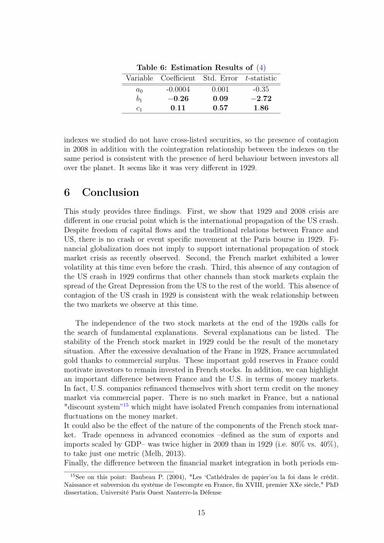
Table 6: Estimation Results of (4)Variable Coefficient Std. Error t-statistic

a0 -0.0004 0.001 -0.35b1 −0.26 0.09 −2.72c1 0.11 0.57 1.86

indexes we studied do not have cross-listed securities, so the presence of contagionin 2008 in addition with the cointegration relationship between the indexes on thesame period is consistent with the presence of herd behaviour between investors allover the planet. It seems like it was very different in 1929.

6 Conclusion

This study provides three findings. First, we show that 1929 and 2008 crisis aredifferent in one crucial point which is the international propagation of the US crash.Despite freedom of capital flows and the traditional relations between France andUS, there is no crash or event specific movement at the Paris bourse in 1929. Fi-nancial globalization does not imply to support international propagation of stockmarket crisis as recently observed. Second, the French market exhibited a lowervolatility at this time even before the crash. Third, this absence of any contagion ofthe US crash in 1929 confirms that other channels than stock markets explain thespread of the Great Depression from the US to the rest of the world. This absence ofcontagion of the US crash in 1929 is consistent with the weak relationship betweenthe two markets we observe at this time.

The independence of the two stock markets at the end of the 1920s calls forthe search of fundamental explanations. Several explanations can be listed. Thestability of the French stock market in 1929 could be the result of the monetarysituation. After the excessive devaluation of the Franc in 1928, France accumulatedgold thanks to commercial surplus. These important gold reserves in France couldmotivate investors to remain invested in French stocks. In addition, we can highlightan important difference between France and the U.S. in terms of money markets.In fact, U.S. companies refinanced themselves with short term credit on the moneymarket via commercial paper. There is no such market in France, but a national"discount system”15 which might have isolated French companies from internationalfluctuations on the money market.It could also be the effect of the nature of the components of the French stock mar-ket. Trade openness in advanced economies –defined as the sum of exports andimports scaled by GDP– was twice higher in 2009 than in 1929 (i.e. 80% vs. 40%),to take just one metric (Melh, 2013).Finally, the difference between the financial market integration in both periods em-

15See on this point: Baubeau P. (2004), "Les ‘Cathédrales de papier’ou la foi dans le crédit.Naissance et subversion du système de l’escompte en France, fin XVIII, premier XXe siècle," PhDdissertation, Université Paris Ouest Nanterre-la Défense

15

phasized in the paper could be completed by an analysis in terms of interest rateparity.

7 References

Annaert and al. (2011), « Are blue chip stock market indices good proxies forall-shares market indices? The case of the Brussels Stock Exchange 1833-2005 »,Financial History Review.

Almunia, M., Bénétrix, A., Eichengreen, B., O’Rourke, K. H., and G. Rua (2010),From Great Depression to Great Credit Crisis: similarities, differences and lessons,Economic Policy, 25(62), pp. 219-265.

Baubeau P. (2004), "Les ‘Cathédrales de papier’ou la foi dans le crédit. Naissanceet subversion du système de l’escompte en France, fin XVIII, premier XXe siècle,"PhD dissertation, Université Paris Ouest Nanterre-la Défense

Bordo, M. and Murshid A. P. (2000), Are Financial Crises Becoming IncreasinglyMore Contagious? What is the Historical Evidence on Contagion?, NBER WorkingPaper No.7900.

Chien-Chung N. and Cheng-Few L. (2001), Dynamic relationship between stockprices and exchange rates for G-7 countries, , The Quarterly Review of Economicsand Finance, 41, pp. 477-490.

Desirier Jean (1930), La bourse de valeur, Revue d’Economie Politique.

Forbes K. and Rigobon R. (2000), Measuring Contagion : Conceptual and EmpiricalIssues, NBER Working paper.

Forbes K. and Rigobon R. (2002), No Contagion, Only Interdependence : MeasuringStock Market Comovements, The Journal of Finance, October, pp. 2223-2261.

Goetzmann, W. N., Lingfeng L., Geert R. (2001), Long-Term Global Market Corre-lations, NBER Working Paper No. 8612.

Grossman Richard S., Meissner Christopher M. (2010), International Aspects ofthe Great Depression and the Crisis of 2007: Similarities, Differences, and Lessons,NBER Working Paper No. 16269.

Jacques, R. (1932), Paris peut-il remplacer Londres comme Marché financier inter-national ?, Revue d’Economie Politique, janvier-février 1932.

Landes D. (2000), L’Europe technicienne, Paris, Gallimard.

Le Bris D. and Hautcoeur P. C.(2010), A challenge to triumphant optimists? A bluechips index for the Paris stock exchange, 1854-2007, Financial History Review.

Le Bris, D. (2012), La volatilité des actions françaises sur le long terme, RevueEconomique, 63.3, pp. 569-580.

Mauro, Paolo, Nathan Sussman and Yishay Yafeh (2002), “Emerging Market Spreads:Then Versus Now,” Quarterly Journal of Economics, 117.2, pp. 695-733.

16

Mauro, Paolo, Nathan Sussman and Yishay Yafeh (2006), Emerging Markets andFinancial Globalization: Sovereign Bond Spreads in 1870-1913 and Today, Oxford,Oxford University Press.

Masih, A. M. and Masih, R. (1997), Dynamic Linkages and the Propagation Mech-anism Driving Major International Stock Markets: An Analysis of the Pre- andPost-Crash Eras, The Quarterly Review of Economics and Finance, Vol 37, No. 4,Fall 1997.

Melh Arnaud (2013), Large Global Volatility Shocks, Equity Markets and Globali-sation 1885-2011, ECB Working Paper No. 1548.

Mitchener K. J. and Wandschneider K. (2014), Capital Controls and Recovery Fromthe Financial Crisis of the 1930s, NBER Working paper No. 20220.

Obstfeld M., Taylor A. M. (1997), The Great Depression as a Watershed: Interna-tional Capital Mobility Over the Long Run, NBER Working Paper No. 5960.

Peicuti, C. (2014), The Great Depression and the Great Recession: A comparativeAnalysis of their Analogies, MPRA Working paper No. 57883.

Sauvy A. (1984), Histoire économique de la France entre les deux guerres, volume3, Paris, Economica.

Schwert, G. (1997), “Stock Market Volatility: Ten Years after the Crash”, NBERWorking paper No. 6381.

17

Appendix 1

Table 7: Index CompositionShare in Number of Price on Market

Security the index shares January 4th 1929 capitalizationCanal maritime de Suez 17,87% 446 796 24 600 10 991 181 600Banque de France 6,97% 182 500 23 500 4 288 750 000Saint Gobain 5,44% 410 000 8 160 3 345 600 000Crédit Foncier de France 4,88% 600 000 5 000 3 000 000 000Brasseries Argentine Quilmès 3,53% 240 000 9 040 2 169 600 000Mines de Lens SC 3,37% 2 050 000 1 010 2 070 500 000Banque de Paris et des Pays-Bas 3,34% 400 000 5 140 2 056 000 000Crédit Lyonnais 3,32% 500 000 4 090 2 045 000 000Banque de l’Indo-Chine 3,24% 144 000 13 850 1 994 400 000Société Générale 3,06% 1 000 000 1 880 1 880 000 000Produits chimiques d’Alais et Camargue 2,71% 400 000 4 170 1 668 000 000Mines de Courrières 2,48% 1 080 000 1 411 1 523 880 000Nord (Chemins de fer) 1,96% 525 000 2 300 1 207 500 000Mines de Marles 1,96% 1 040 000 1 160 1 206 400 000Comptoir Nationale d’Escompte 1,91% 500 000 2 355 1 177 500 000Paris Lyon Méditérannée 1,90% 800 000 1 460 1 168 000 000Mines d’Anzin 1,77% 400 600 2 725 1 091 635 000Etb Kuhlmann 1,63% 720 000 1 395 1 004 400 000Banque de l’Union Parisienne 1,56% 300 000 3 190 957 000 000Banque de l’Algérie 1,47% 50 000 18 050 902 500 000Raffinerie Say 1,46% 368 156 2 440 898 300 640Mines d’Aniche 1,41% 320 000 2 715 868 800 000Sarre et Moselle 1,41% 400 000 2 170 868 000 000Houilles de Blanzy 1,40% 600 000 1 435 861 000 000Banque Nationale de Crédit 1,39% 500 000 1 705 852 500 000Cie Parisienne de distribution d’électricité 1,39% 400 000 2 130 852 000 000Sté Lyonnaise des Eaux et d’Eclairage AJ 1,38% 250 000 3 390 847 500 000Mines de Vicoigne et Noeux SC 1,35% 600 000 1 380 828 000 000Charbonnages du Tonkin 1,33% 64 000 12 800 819 200 000Union d’électricité 1,31% 800 000 1 008 806 400 000Air Liquide 1,30% 600 000 1 335 801 000 000Penarroya 1,28% 585 000 1 345 786 825 000Orléans (Chemins de fer) 1,22% 600 000 1 255 753 000 000Cie de Béthune 1,19% 85 000 8 600 731 000 000Forges et Aciéries du Nord et de l’Est 1,18% 440 000 1 655 728 200 000Citroën 1,14% 400 000 1 760 704 000 000Mines de Dourges SC 1,14% 285 000 2 460 701 100 000Est-Lumière 1,13% 675 000 1 026 692 550 000Ouest Parisien 1,12% 840 000 820 688 800 000Est (Chemins de fer) 1,10% 584 000 1 160 677 440 000Total 100% 61 513 462 24

Notes: In francs. Source: Authors.

18

Figure 5: Sub-indices in 1929

Notes: base 1929M02=100. Source: calculation from authors

Table 8: Sub-Indices (Industrial, Banks) vs. Total (HCAC 40) index

Mean VarianceVariable t-test F -testIndustrial -0.149 1.364

(0.88) (0.007)

Banks 0.260 1.219(0.79) (0.08)

Notes: Tests were applied on stationary data. a denotesrejection of the null of equality in mean (or variance). p-values are reported in parentheses.

Appendix 2

19

Figure 6: Stock returns volatility in 1929

Figure 7: Stock returns volatility in 2008

Appendix 3• The Great RecessionBoth series in levels seem to have a downward trend. Regarding the unit root tests,there are both I(1), we can then suppose there is a constant term in the error cor-rection model.

20

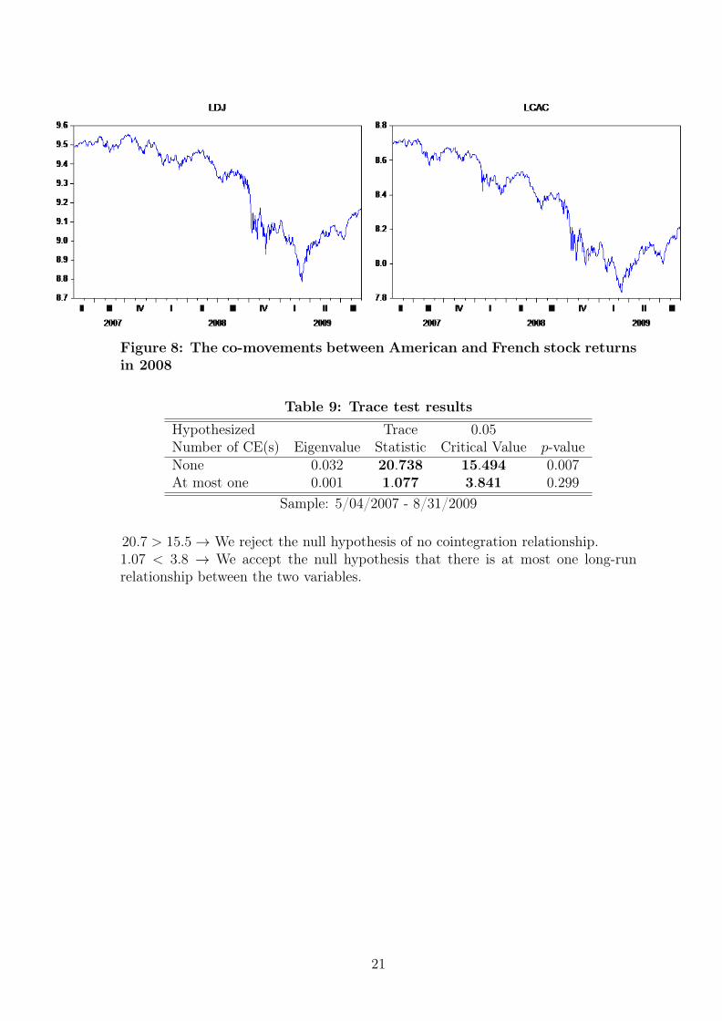
Figure 8: The co-movements between American and French stock returnsin 2008

Table 9: Trace test results

Hypothesized Trace 0.05Number of CE(s) Eigenvalue Statistic Critical Value p-valueNone 0.032 20.738 15.494 0.007At most one 0.001 1.077 3.841 0.299

Sample: 5/04/2007 - 8/31/2009

20.7 > 15.5→ We reject the null hypothesis of no cointegration relationship.1.07 < 3.8 → We accept the null hypothesis that there is at most one long-runrelationship between the two variables.

21

Table 10: Vector Error Correction Estimates

Cointegrating Equation zt−1

LCACt−1 1LDJt−1 -1.185

(0.056)

Intercept 2.649Error Correction ∆LCAC ∆LDJ

zt−1 -0.041 0.004(0.013) (0.018)

∆LCACt−1 -0.456 -0.044(0.040) (0.055)

∆LCACt−2 -0.030 -0.025(0.027) (0.038)

∆LDJt−1 0.827 -0.159(0.033) (0.046)

∆LDJt−2 0.355 -0.092(0.044) (0.061)

Intercept -0.0005 -0.0007(0.0005) (0.0007)

Sample 5/7/2007 - 8/31/2009 (606 observations)R-squared 0.58 0.04F -stat 170.60 5.11AIC -5.77 -5.13Notes: standard errors are reported in brackets.

• The Great Depression

Table 11: Trace test results

Hypothesized Trace 0.05Number of CE(s) Eigenvalue Statistic Critical Value p-valueNone 0.015 7.169 15.497 0.558At most one 0.008 2.541 3.841 0.111

Sample: 2/05/1929 - 3/31/1930

27.17 < 15.5 → We accept the null hypothesis at the 5% confidence level, thusthere is no cointegration.

22

Table 12: Pairwise Granger causality test

Number of lags p = 1 p = 2 p = 3 p = 4 p = 5 p = 6RDJ → RCAC < 0.01 0.481 0.264 0.377 0.374 0.451RCAC → RDJ < 0.01 < 0.01 < 0.01 < 0.01 < 0.01 < 0.01Notes: the probabilities of incorrectly rejecting the null of no causality are reported above.

Table 13: VAR(3) Estimates

∆LDJ ∆LHCAC

∆LDJt−1 0.215 0.184(0.056) (0.034)

∆LDJt−2 -0.352 -0.007(0.056) (0.034)

∆LDJt−3 0.265 0.011(0.058) (0.035)

∆LHCACt−1 -0.131 -0.227(0.097) (0.058)

∆LHCACt−2 -0.129 -0.014(0.099) (0.059)

∆LHCACt−3 0.071 -0.074(0.092) (0.055)

Intercept -0.0004 -0.0006(0.0001) (0.0007)

Sample 2/07/1929 - 3/31/1930 (298 obs.)R-squared 0.19 0.14F -stat 12.11 8.21AIC -4.83 -5.84Notes: standard errors are reported in brackets.

Table 14: VAR(1) Estimates

∆LDJ ∆LHCAC

∆LDJt−1 0.106 0.184(0.057) (0.032)

∆LHCACt−1 -0.259 –0.255(0.095) (0.052)

Intercept -0.0004 -0.0005(0.001) (0.0007)

Sample 2/05/1929 - 3/31/1930 (300 obs.)R-squared 0.03 0.15F -stat 5.04 26.48AIC -4.67 -5.82Notes: standard errors are reported in brackets.

23