unsteady axial flows of upper-convected maxwell fluid in …15) 1 - 16.pdf · unsteady axial flows...

Arab Journal of Nuclear Science and Applications, 94 (4), (129-141) 2016

921

Unsteady Axial Flows of Upper-Convected Maxwell Fluid in Pipe

M. Saleh Yousef1,2, M. H. M. Soleiman2, and A. M. O. Elshini2,* (1)Department of Physics, Taibah University, Almadinah Almunawwarah, Saudi Arabia

(2)Department of Physics, Cairo University, Giza 12613, Egypt

Received: 5/11/2015 Accepted: 4/1/2016

ABSTRACT1

The present research involves an analytical examination of the unsteady

axial flow of an incompressible viscoelastic upper-convected Maxwell fluid

through a straight tube of circular cross-section in the absence of external

forces. The flow is considered initially at rest and the flow pattern is

investigated through the velocity profiles for four cases of pressure -gradient field: (i) Constant pressure-gradient, (ii) Exponentially rising pressure-

gradient with time, (iii) Exponentially falling pressure-gradient with time, and

(iv) Periodic pressure-gradient. Fourier-Bessel series solution is assumed in a

general form for the velocity field. The integral-transforms and the inverse

derivative technique are used to obtain the exact solution of the considered

initial-boundary value problem. The limiting flow of the Newtonian fluids is

well described in this approach by removing the relaxation-time dependence. The velocity profiles have been determined.

Keywords: Upper-Convected Maxwell Fluid / Viscoelastic / Circularcross-section

/Fourier-BesselSeries / Periodic Pressure-Gradient / Traverse-Time.

1- INTRODUCTION

The study of the pipe flows of fluids is of immense importance and serves a wide variety of practical applications, e.g. food, chemical, petroleum, mechanical, material processing, and nuclear industries. The simplest rheological studies are carried out on the Newtonian fluids as Newton’s law for the viscous fluids exhibits a direct proportionality between stress and strain rate in laminar flow for which the constitutive law is,

𝐓 = 𝜇𝐃 (1)

The stress T versus the strain rate D graph presents a straight line that passes the origin and the

viscosity𝜇is independent of the strain rate although it may be affected by other physical parameters, e.g. temperature and pressure, for a studied fluid system(1). The unsteady pipe flows of Newtonian fluids have been studied by several authors, e.g.(2–6). In practice, the applications of Newtonian fluid are limited as very few fluids obey Newton’s law of viscosity. Moreover, there are several fluids of importance, both in technology and in nature, that deviate greatly from Newtonian fluid in behavior which and are called non-linear viscoelastic fluids. Many authors studied those fluids (7–11). Pascal and Pascal(7) studied the power-law fluid and formulated it using non-linear shear flows of non-Newtonian fluids. Dabe et al.(8) studied Rivlin-Ericksen fluid in tube of a little deformation in cross-section with mass and heat transfer. Avinash et al.(9) studied Bingham fluid flow through a tapered tube with a permeable wall. Tong et al.(10) studied unsteady helical flows of a generalized Oldroyd-B fluid. Kamran et al.(11) obtained exact solutions for the unsteady rotational flow of a generalized second grade fluid through a circular cylinder. The upper-convected Maxwell (UCM) fluid is a non-linear viscoelastic fluid model, which exhibits a simple combination of the Newton’s law for viscous fluids and the derivative of Hook’s law for elastic solids(12).

1Corresponding author e-mail:[email protected]


931

The channel and pipe flows of Maxwell fluid have been studied by several authors (13–19). Zidan(13) studied the unsteady flow of viscoelastic fluid in confocal elliptic cylinders. Yin and Zhu(14) investigated the oscillating flow of a viscoelastic fluid in a pipe with the fractional Maxwell model. Qi and Jin(15) studied the unsteady rotating flows of a viscoelastic fluid with the fractional Maxwell model between coaxial cylinders. Miranda and Oliveira (16) determined the start-up times in viscoelastic channel and pipe flows. Wang et al.(17) investigated the transient electro-osmotic flow of generalized Maxwell fluids in a straight pipe of circular cross-section. Zhou and Hou(18)used the least-squares finite element method to solve the steady upper-convected Maxwell fluid.Jiméneza et al.(19)

investigated the start-up electro-osmotic flow of Maxwell fluids in a rectangular microchannel with high zeta potentials.

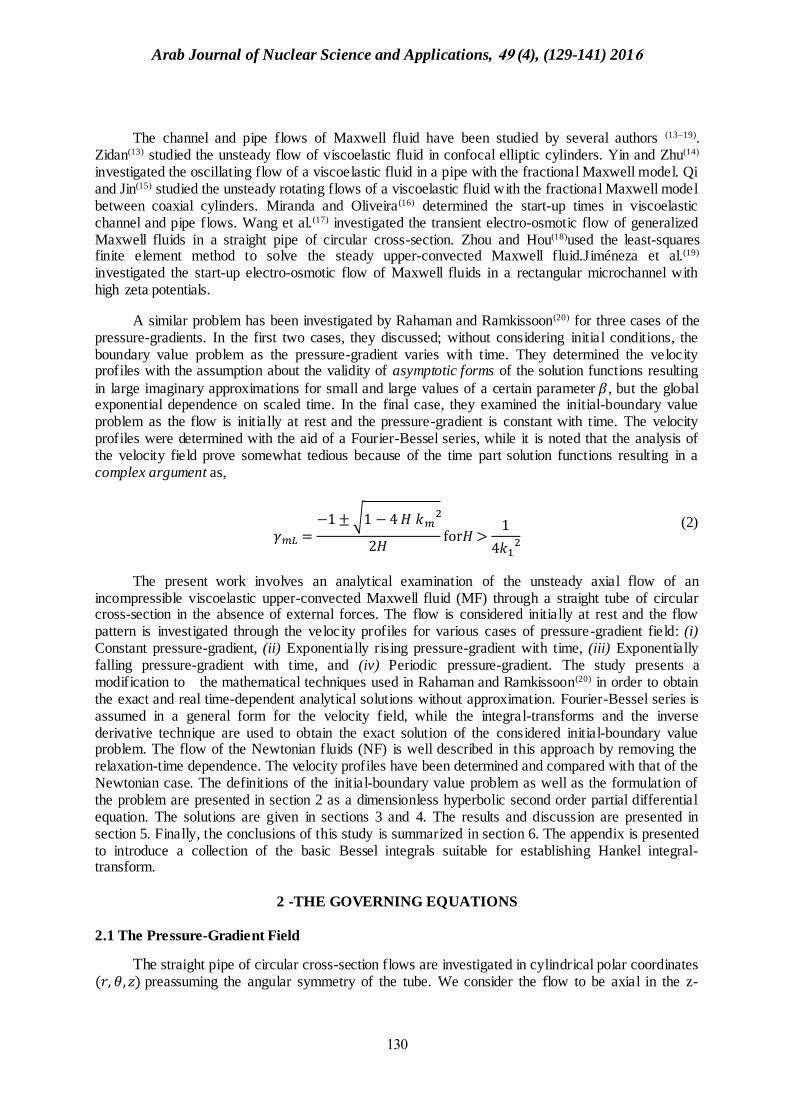
A similar problem has been investigated by Rahaman and Ramkissoon(20) for three cases of the pressure-gradients. In the first two cases, they discussed; without considering initial conditions, the boundary value problem as the pressure-gradient varies with time. They determined the velocity profiles with the assumption about the validity of asymptotic forms of the solution functions resulting

in large imaginary approximations for small and large values of a certain parameter 𝛽, but the global exponential dependence on scaled time. In the final case, they examined the initial-boundary value problem as the flow is initially at rest and the pressure-gradient is constant with time. The velocity profiles were determined with the aid of a Fourier-Bessel series, while it is noted that the analysis of the velocity field prove somewhat tedious because of the time part solution functions resulting in a complex argument as,

𝛾𝑚𝐿 =−1 ± √1 − 4 𝐻 𝑘𝑚

2

2𝐻for𝐻 >

1

4𝑘12

(2)

The present work involves an analytical examination of the unsteady axial flow of an incompressible viscoelastic upper-convected Maxwell fluid (MF) through a straight tube of circular cross-section in the absence of external forces. The flow is considered initially at rest and the flow pattern is investigated through the velocity profiles for various cases of pressure-gradient field: (i) Constant pressure-gradient, (ii) Exponentially rising pressure-gradient with time, (iii) Exponentially falling pressure-gradient with time, and (iv) Periodic pressure-gradient. The study presents a modification to the mathematical techniques used in Rahaman and Ramkissoon(20) in order to obtain the exact and real time-dependent analytical solutions without approximation. Fourier-Bessel series is assumed in a general form for the velocity field, while the integral-transforms and the inverse derivative technique are used to obtain the exact solution of the considered initial-boundary value problem. The flow of the Newtonian fluids (NF) is well described in this approach by removing the relaxation-time dependence. The velocity profiles have been determined and compared with that of the Newtonian case. The definitions of the initial-boundary value problem as well as the formulation of the problem are presented in section 2 as a dimensionless hyperbolic second order partial differential equation. The solutions are given in sections 3 and 4. The results and discussion are presented in section 5. Finally, the conclusions of this study is summarized in section 6. The appendix is presented to introduce a collection of the basic Bessel integrals suitable for establishing Hankel integral-transform.

2 -THE GOVERNING EQUATIONS

2.1 The Pressure-Gradient Field

The straight pipe of circular cross-section flows are investigated in cylindrical polar coordinates (𝑟, 𝜃, 𝑧) preassuming the angular symmetry of the tube. We consider the flow to be axial in the z-


939

direction which implies that the pressure acts on the fluid parcel parallel to the tube axis and thus the

pressure-gradient field −𝛁𝑝 (𝑧, 𝑡) will have the form,

−𝛁 𝑝(𝑧, 𝑡) = (0,0, −𝜕𝑧 𝑝(𝑧, 𝑡)) (3)

2.2 The Continuity Equation

We assume that the fluid under consideration is incompressible(21,22) for which the continuity equation reads:

𝛁 . 𝐯 = 0, (4) then, the axial flow velocity field will have the form,

𝐯 = (0,0, 𝜔(𝑟, 𝑡)), (5)

where𝜔(𝑟, 𝑡) is the axial flow speed.

2.3 The Dynamical Equation

In the absence of external forces, Cauchy’s first law of motion(21,22) for a fluid parcel reads;

𝜌𝐷𝑡𝐯 = 𝛁. 𝐓, (6)

𝐓 = −𝑝𝐈 + 𝐒. (7)

where 𝜌 is the fluid mass density, 𝐓 is the tensor of the total stress field acting on the fluid, 𝐒 is the tensor of the extra (friction) stress field due to the fluid viscosity, 𝑝 is the isotropic pressure field, 𝐈 is the identity matrix and 𝐷𝑡 is a generalized differentiation operator. The dynamical equations are obtained by substitution of Eqs. (3), (5) and (7) into Eq. (6) which yield the system of equations, 𝜕𝑧𝑆𝑟𝑧 = 0, (8)

𝜌𝜕𝑡 𝜔(𝑟, 𝑡) − (𝜕𝑟 +1

𝑟)𝑆𝑧𝑟 −

1

𝑟𝜕𝜃𝑆𝑧𝜃 − 𝜕𝑧𝑆𝑧𝑧 = −𝜕𝑧𝑝(𝑧, 𝑡).

(9)

where the initial conditions are, 𝜔(𝑟, 0) = 0 and𝜕𝑡𝜔(𝑟, 0) = 0 for0 ≤ 𝑟 ≤ 𝑅 (10)

and the boundary conditions are, 𝜔(𝑅, 𝑡) = 0 and𝜕𝑟𝜔(0, 𝑡) = 0 for 0 ≤ 𝑡 ≤ 𝑇 (11)

where 𝑅 and 𝑇 are the radius of the tube and the scaling time, respectively. 2.4 The Constitutive Equations:

We take the upper-convected Maxwell fluid(23–25) to be the fluid model of the study for which

the rheological equation of state is, ∇

𝐒 + 𝜆𝐒= 2𝜇𝐃

(12)

where the upper-convected derivative of the extra stress tensor∇𝐒 and the deformation rate tensor 𝐃 are

defined as, ∇

𝐒 = 𝐷𝑡𝐒 − [𝐒 . (𝛁𝐯) + (𝛁𝐯)T . 𝐒],

(13)

𝐃 =1

2[𝛁𝐯 + (𝛁𝐯)T].

(14)


932

while 𝜆 is the relaxation-time, 𝜇 is the viscosity coefficient and (. ) 𝑇 is the matrix transpose operation. The substitutions by Eq. (5) into Eqs. (13) and (14) then by the modified Eqs. (13) and (14) into Eq. (12) yield the constitutive equations; (𝜆𝜕𝑡 + 1)𝑆𝑧𝑟 = 𝜇𝜕𝑟𝜔(𝑟, 𝑡), (15)

(𝜆𝜕𝑡 + 1)𝑆𝑧𝑧 = 2𝜆𝑆𝑧𝑟𝜕𝑟𝜔(𝑟, 𝑡). (16)

2.5 The Equation of Motion

The equation of motion is easily obtained via eliminating the S-components between the

constitutive and dynamical equations,

𝜌(𝜆𝜕𝑡2 + 𝜕𝑡)𝜔(𝑟, 𝑡) − 𝜇 (𝜕𝑟

2 +1

𝑟𝜕𝑟) 𝜔(𝑟, 𝑡) = (𝜆𝜕𝑡 + 1)(−𝜕𝑧𝑝(𝑧, 𝑡))

(17)

The above equation is transformed a into non-dimensional form by introducing the following scaled variables,

𝜂 = (1

𝑅) 𝑟, ℎ = (

1

𝐿) 𝑧,

𝜏 = (

𝜇

𝜌𝑅2)𝑡, 𝐻 = (

𝜇

𝜌𝑅2)𝜆,

𝜙(𝜂, 𝜏) = (

𝜌𝑅

𝜇) 𝜔(𝑟, 𝑡), 𝑔(ℎ, 𝜏) = (

𝜌𝑅2

𝜇2)𝑝(𝑧, 𝑡).

where 𝑅 and 𝐿 are the radius and length of the tube. Hence the scaled equation of motion becomes,

(𝐻𝜕𝜏2 + 𝜕𝜏)𝜙(𝜂, 𝜏) −

1

𝜂𝜕𝜂 (𝜂𝜕𝜂𝜙(𝜂, 𝜏)) = 𝑓(𝜏)

(18)

This is a hyperbolic partial differential equation for a scaled velocity field. The initial-boundary conditions appropriate for our study are, 𝜙(𝜂, 0) = 0 and𝜕𝜏𝜙(𝜂, 0) = 0 for 0 ≤ 𝜂 ≤ 1, (19) 𝜙(1, 𝜏) = 0 and𝜕𝜂𝜙(0, 𝜏) = 0 for 0 ≤ 𝜏 ≤ 1. (20)

The first equation expresses the no-slippage condition of the interaction of the viscoelastic fluid of the tube walls. The second equation fixes the velocity profiles at the tube axis to be of local extreme value.

where 𝑓(𝜏) = (𝐻𝜕𝜏 + 1)𝜋(𝜏) while the pressure-gradient field reads 𝜋(𝜏) = (−𝑅

𝐿) 𝜕ℎ𝑔(ℎ, 𝜏).

3- THE GENERAL FORM OF THE VELOCITY FIELD

We express the velocity field as a Fourier-Bessel series(26),

𝜙(𝜂, 𝜏) = ∑ 𝐴𝑛(𝜏)𝐽0(𝜁𝑛𝜂),

∞

𝑛=1

(21)

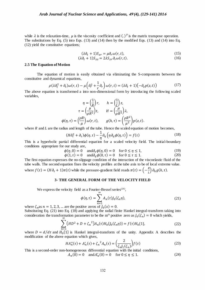
where 𝜁𝑛as 𝑛 = 1, 2, 3, … are the positive zeros of 𝐽0(𝑥) = 0. Substituting Eq. (21) into Eq. (18) and applying the radial finite Hankel integral-transform taking into

consideration the transformation parameter to be the mth positive zero as 𝐽0(𝜁𝑛) = 0 which yields,

∑(𝐻𝐷2 + 𝐷 + 𝜁𝑛2)𝐴𝑛(𝜏)𝐻0{𝐽0(𝜁𝑛𝜂)}

∞

𝑛=1

= 𝑓(𝜏)𝐻0{1},

(22)

where 𝐷 = 𝑑 𝑑𝜏⁄ and 𝐻0{1} is Hankel integral-transform of the unity. Appendix A describes the modification of the above equation which gives,

𝐻𝐴𝑛′′(𝜏) + 𝐴𝑛

′ (𝜏) + 𝜁𝑛2𝐴𝑛(𝜏) = (

2

𝜁𝑛𝐽1(𝜁𝑛))𝑓(𝜏)

(23)

This is a second-order non-homogeneous differential equation with the initial conditions, 𝐴𝑛(0) = 0 and𝐴𝑛

′ (0) = 0 for 0 ≤ 𝜂 ≤ 1. (24)


933

The auxiliary equation of Eq. (23) exhibits complex roots and the general solution reads, 𝐴𝑛(𝜏) = 𝑒𝛽𝜏 (𝐵𝑛 cos𝛾𝑛𝜏 + 𝐶𝑛 sin 𝛾𝑛𝜏) + 𝜓𝑛(𝜏) (25)

where 𝛽 = −

1

2𝐻,

𝛾𝑛 =√4𝐻𝜁𝑛

2 − 1

2𝐻for 𝐻 >

1

4𝜁12 .

The particular solution 𝜓𝑛(𝜏) is obtained via the inverse derivative technique(27) which reads,

𝜓𝑛(𝜏) = (2

𝜁𝑛𝐽1(𝜁𝑛))[𝐹(𝐷)]−1 𝑓(𝜏),

(26)

Where the differential operator is 𝐹(𝐷) = 𝐻𝐷2 + 𝐷 + 𝜁𝑛2

and the inverse differential operator 1 𝐹(𝐷)⁄ or[𝐹(𝐷)]−1 is defined as 𝐹(𝐷)[𝐹(𝐷)]−1𝑓(𝜏) = 𝑓(𝜏), see(27).

The evaluation of the integration constants 𝐵𝑛 and 𝐶𝑛 implies applying the initial conditions in Eq. (24), 𝐵𝑛 = −𝑘𝑛, (27)

𝐶𝑛 =𝛽𝑘𝑛 − 𝜓𝑛

′ (0)

𝛾𝑛,

(28)

where 𝑘𝑛 = 𝜓𝑛(0). Finally, the MF-velocity field will have the general form,

𝜙(𝜂, 𝜏) = ∑ {𝜓𝑛(𝜏) − 𝑒𝛽𝜏 [𝑘𝑛 cos𝛾𝑛𝜏 − (𝛽𝑘𝑛 − 𝜓𝑛

′ (0)

𝛾𝑛

)sin 𝛾𝑛𝜏]}𝐽0(𝜁𝑛𝜂)

∞

𝑛=1

(29)

4- THE VELOCITY PROFILES

4.1 The Constant Pressure-Gradient with Time

Over the flow time interval, the pressure-gradient is considered to be constant with the form, 𝜋(𝜏) = 𝑘, (30) 𝑓(𝜏) = 𝑘. (31)

𝜓𝑛(𝜏) is determined via the inverse derivative technique(27) and the binomial theorem(26), knowing

that(1 + 𝑥)−1 = ∑ (−1)𝑛𝑥𝑛∞𝑛=0 , which yields,

𝜓𝑛(𝜏) = 𝑘𝑛, (32) 𝜓𝑛

′ (0) = 0. (33)

The resulting MF-velocity field is then,

𝜙(𝜂, 𝜏) = ∑ 𝑘𝑛(1 − 𝑒𝛽𝜏[cos𝛾𝑛𝜏 + 𝐷𝑛 sin 𝛾𝑛𝜏])𝐽0(𝜁𝑛𝜂)

∞

𝑛=1

(34)

Finally, the NF-velocity field readily becomes,

��(𝜂, 𝜏) = ∑ 𝑘𝑛(1 − 𝑒−𝜁2𝜏)𝐽0(𝜁𝑛𝜂)

∞

𝑛=1

,

(35)

where 𝑘𝑛 =

2𝑘

𝜁𝑛3𝐽1(𝜁𝑛)

,

𝐷𝑛 = − (

𝛽

𝛾𝑛

).

4.2 The Rising Pressure-Gradient with Time

We consider the pressure-gradient is rising exponentially as, 𝜋(𝜏) = 𝑘𝑒𝛼𝜏 , (36)


931

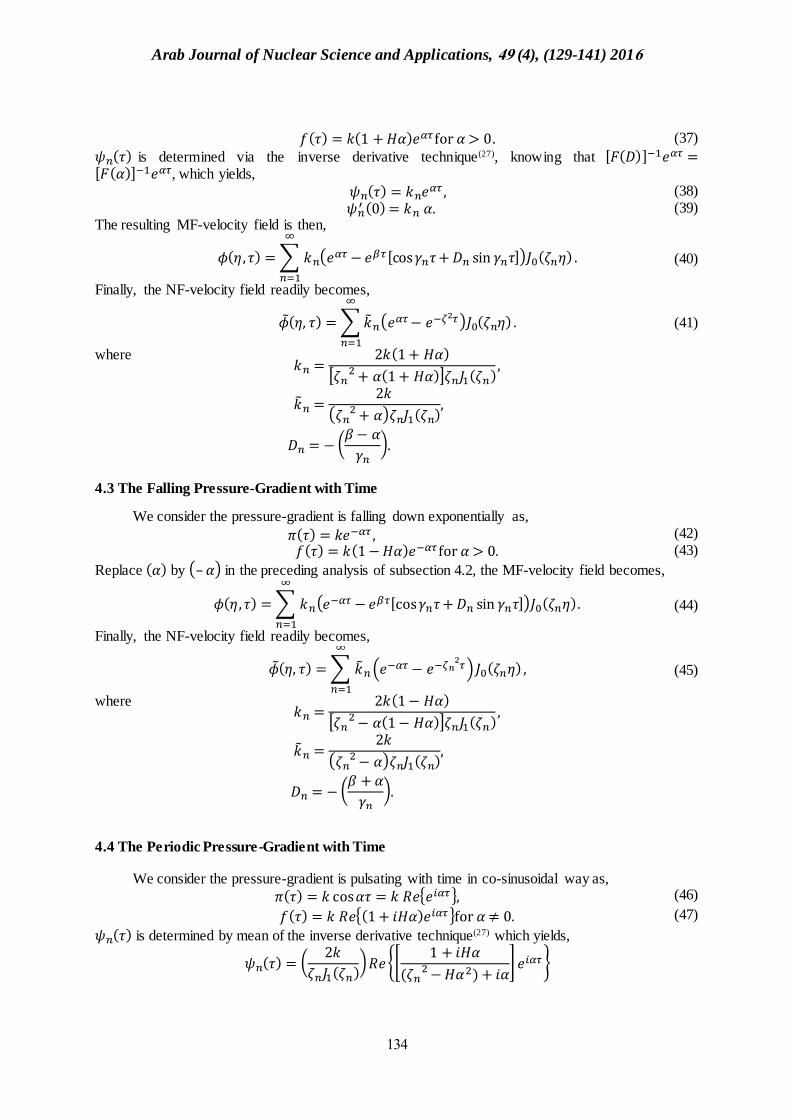
𝑓(𝜏) = 𝑘(1 + 𝐻𝛼)𝑒𝛼𝜏 for 𝛼 > 0. (37)

𝜓𝑛(𝜏) is determined via the inverse derivative technique(27), knowing that [𝐹(𝐷)]−1𝑒𝛼𝜏 =[𝐹(𝛼)]−1𝑒𝛼𝜏, which yields, 𝜓𝑛(𝜏) = 𝑘𝑛𝑒𝛼𝜏 , (38) 𝜓𝑛

′ (0) = 𝑘𝑛 𝛼. (39) The resulting MF-velocity field is then,

𝜙(𝜂, 𝜏) = ∑ 𝑘𝑛(𝑒𝛼𝜏 − 𝑒𝛽𝜏 [cos𝛾𝑛𝜏 + 𝐷𝑛 sin 𝛾𝑛𝜏])𝐽0(𝜁𝑛𝜂)

∞

𝑛=1

.

(40)


��(𝜂, 𝜏) = ∑ ��𝑛(𝑒𝛼𝜏 − 𝑒−𝜁2𝜏)𝐽0(𝜁𝑛𝜂)

∞

𝑛=1

.

(41)

where 𝑘𝑛 =

2𝑘(1 + 𝐻𝛼)

[𝜁𝑛2 + 𝛼(1 + 𝐻𝛼)]𝜁𝑛𝐽1(𝜁𝑛)

,

��𝑛 =

2𝑘

(𝜁𝑛2 + 𝛼)𝜁𝑛𝐽1(𝜁𝑛)

,

𝐷𝑛 = − (

𝛽 − 𝛼

𝛾𝑛

).

4.3 The Falling Pressure-Gradient with Time

We consider the pressure-gradient is falling down exponentially as, 𝜋(𝜏) = 𝑘𝑒−𝛼𝜏 , (42) 𝑓(𝜏) = 𝑘(1 − 𝐻𝛼)𝑒−𝛼𝜏 for 𝛼 > 0. (43)

Replace (𝛼) by (– 𝛼) in the preceding analysis of subsection 4.2, the MF-velocity field becomes,

𝜙(𝜂, 𝜏) = ∑ 𝑘𝑛(𝑒−𝛼𝜏 − 𝑒𝛽𝜏[cos𝛾𝑛𝜏 + 𝐷𝑛 sin 𝛾𝑛𝜏])𝐽0(𝜁𝑛𝜂)

∞

𝑛=1

.

(44)


��(𝜂, 𝜏) = ∑ ��𝑛 (𝑒−𝛼𝜏 − 𝑒−𝜁𝑛2

𝜏 )𝐽0(𝜁𝑛𝜂)

∞

𝑛=1

,

(45)

where 𝑘𝑛 =

2𝑘(1 − 𝐻𝛼)

[𝜁𝑛2 − 𝛼(1 − 𝐻𝛼)]𝜁𝑛𝐽1(𝜁𝑛)

,

��𝑛 =

2𝑘

(𝜁𝑛2 − 𝛼)𝜁𝑛𝐽1(𝜁𝑛)

,

𝐷𝑛 = − (

𝛽 + 𝛼

𝛾𝑛

).

4.4 The Periodic Pressure-Gradient with Time

We consider the pressure-gradient is pulsating with time in co-sinusoidal way as, 𝜋(𝜏) = 𝑘 cos𝛼𝜏 = 𝑘 𝑅𝑒{𝑒𝑖𝛼𝜏 }, (46)

𝑓(𝜏) = 𝑘 𝑅𝑒{(1 + 𝑖𝐻𝛼)𝑒𝑖𝛼𝜏 }for 𝛼 ≠ 0. (47)

𝜓𝑛(𝜏) is determined by mean of the inverse derivative technique(27) which yields,

𝜓𝑛(𝜏) = (2𝑘

𝜁𝑛𝐽1(𝜁𝑛))𝑅𝑒{[

1 + 𝑖𝐻𝛼

(𝜁𝑛2 − 𝐻𝛼2) + 𝑖𝛼

] 𝑒𝑖𝛼𝜏 }


931

Using Euler's identities for the relationship between exponential and trigonometric functions (28) for the

complex argument 𝑒𝑖𝛼𝜏 and multiplying by the self conjugate of (𝜁𝑛2 − 𝐻𝛼2) + 𝑖𝛼, we get,

𝜓𝑛(𝜏) = 𝑘𝑛(cos𝛼𝜏 + 𝑅𝑛 sin 𝛼𝜏), (48) 𝜓𝑛

′ (0) = 𝑘𝑛𝑅𝑛 𝛼. (49) The resulting MF-velocity field is then,

𝜙(𝜂, 𝜏) = ∑ 𝑘𝑛(cos𝛼𝜏 + 𝑅𝑛 sin 𝛼𝜏 − 𝑒𝛽𝜏[cos𝛾𝑛𝜏 + 𝐷𝑛 sin 𝛾𝑛𝜏])𝐽0(𝜁𝑛𝜂)

∞

𝑛=1

.

(50)


��(𝜂, 𝜏) = ∑ ��𝑛 (cos𝛼𝜏 + ��𝑛 sin 𝛼𝜏 − 𝑒−𝜁𝑛

2𝜏 )𝐽0(𝜁𝑛𝜂)

∞

𝑛=1

,

(51)

where 𝑘𝑛 =

2𝑘𝜁𝑛

[(𝜁𝑛2 − 𝐻𝛼2)

2+ 𝛼2]𝐽1 (𝜁𝑛)

,

��𝑛 =2𝑘𝜁𝑛

(𝜁𝑛4 + 𝛼2)𝐽1(𝜁𝑛)

,

𝑅𝑛 = −𝛼 (

𝐻𝜁𝑛2 − 𝐻2𝛼2 − 1

𝜁𝑛2 ),

��𝑛 =𝛼

𝜁𝑛2,

𝐷𝑛 = − (

𝛽 − 𝛼𝑅𝑛

𝛾𝑛

).

5- RESULTS AND DISCUSSION

It was found that the velocity profile depends to an extent on the radial distance 𝜂and we investigate it at short and long times after the flow start. Fig.(1) shows a plot of the solutions for the four cases with the parameters given in Table (1) of dynamic pressure-gradient.

Table (1): Values of the parameters for each case-study.

Pressure-Gradient 𝑘 𝐻 𝛼

Constant 1.0 0.2 None

Rising 1.0 0.2 1.0

Falling 1.0 0.2 1.0

Periodic 1.0 0.2 2𝜋


931

Fig. (1): Features of pressure-gradient functions when: (a) Constant; (b) Rising; (c) Falling and (d) Periodic over normalized one period

Fig. (1) (a) to (d) shows the behaviors of the four pressure-gradient functions 𝜋(𝜏)used in the present study. Each pressure-gradient behaviour is a case study with distinguishable velocity profile.

A comparison is made between the MF-velocity profiles and those at the limit of NF, keeping for each case the instances of time when the two velocity profiles behave similarly, and obtaining the velocity profiles at short and long times of flow.

The variations of the MF-velocity field 𝜙 are given at two values of the dimensionless radius parameter 𝜂: One along the tube axis (𝜂 = 0) and the other near the tube wall (𝜂 = 0.95); as shown in Figs. (2), (4), (6) and (8). It can be seen from these figures that the velocity profiles for the two fluids become identical at certain times, which we have called traverse-speeds at traverse-times.

5.1 The Constant Pressure-Gradient with Time

In the case of constant pressure-gradient, the traverse-speeds occur at the tube axis and near the walls at only one traverse-time before the maximum velocity ( Fig. (2) (a) and (b)), (Fig. (3) (a) to(d) ) illustrate the time evolution of the profiles along the tube radius to be parabolic.

Moreover , at earlier time, the MF-velocities are smaller than that of NF but they are increasing with time until they become identical. After that the velocities continue increasing till their maximum, they decay then and behave very much like NF at later times. Simpler problem of constant pressure-gradient had been discussed before by Ci-qtm and Jun-qi (29). They examined a simple Maxwell fluid and obtained the analytical solution by means of Hankel integral-transform and its inverse. We obtain the similar behaviors of velocity profile curves (29).


931

Fig. (2): Velocity variations for MF (solid line) and NF (dashed line) when: (a) 𝜂 = 0 and (b) 𝜂 = 0.95~~~~~~~~~~~~~~

Fig. (3): Radial velocity profiles for MF (solid line) and NF (dashed line)

when: (a) 𝜏 = 0.1; (b) 𝜏 = 0.3939; (c) 𝜏 = 0.5 and (d) 𝜏 = 1

5.2 The Rising Pressure-Gradient with Time

The traverse-speeds occur at the tube axis and near the tube walls for only one traverse time before

the half period of time of flow. Fig. (4) (a) and (b) and Fig. (5) (a) to (d) show samples of the time

evolution of the velocity profiles along the tube radius. The profiles are parabolic. At short times, the MF-

velocities are increasing more than that of NF, but, the velocity field nearly behaves like NF at later times.

Fig. (4): Velocity variations for MF (solid line) and NF (dashed line)

when: (a) 𝜂 = 0 and (b) 𝜂 = 0.95~


931



5.3 The Falling Pressure-Gradient with Time

In this case, the traverse-speeds occur at the tube axis and near the tube walls. There are two traverse

times before and after the maximum velocities, see Fig. (6) (a) and (b).

Fig. (6): Velocity variations for MF (solid line) and NF (dashed line)

when: (a) 𝜂 = 0 and (b) 𝜂 = 0.95~ ~~~~~~~~~~~~~

The velocity profiles development with radial distance is obtained for different time instants in Fig.

(7) (a) to (d). The profiles are parabolic. Moreover, the two fluids behave almost similarly at intermediate

times of flow, while the MF-velocity is smaller than that of NF at earlier and later times only.




931

In cases of constant and falling pressure-gradients at a long time, the two fluids have similar velocity profiles, which are asymptotically convergent. Consequently, and as expected, the non-Newtonian effects partially disappear with time. A similar effect had been discussed before by Fetecau et al.(30).

5.4 The Periodic Pressure-Gradient with Time

It was also obtained in this fourth case of the study, the traverse-speeds at the tube axis and near the walls occur at only one traverse time as well as there are phase shifts in the wavy velocity profiles of the two fluids dependent on radial distance, see Fig. (8) (a) and (b).

Fig. (8) Velocity variations for MF (solid line) and NF (dashed line)

when: (a) 𝜂 = 0 and (b) 𝜂 = 0.95~~~~~~~~~~~~~

The velocity profiles along the tube radius are plotted in Fig. (9) (a) to (f) at six time instances taken over one normalized period. The MF shows drop in speed at the tube axis, which becomes a smeared minimum at around half of the one flow period, while the NF-velocity profile behaves as a parabola with global maximum at the tube axis. The flow pattern is shown to be reversed for MF and periodic for NF up to the end of one flow period.

The wall effects on the velocity profile of the two fluids around a circular cylinder were investigated by Huang and Feng (31). They have studied as well the interplay among wall effects, elasticity, shear thinning and inertia for the MF between the parallel walls of the two cylinders and compared it with NF.

Fig. (9): Radial velocity profiles for MF (solid line) and NF (dashed line) over one normalized period

when: (a) 𝜏 = 0.0; (b) 𝜏 = 0.25; (c) 𝜏 = 0.5; (d) 𝜏 = 0.75; (e) 𝜏 = 0.9170 and (f) 𝜏 = 1.0


911

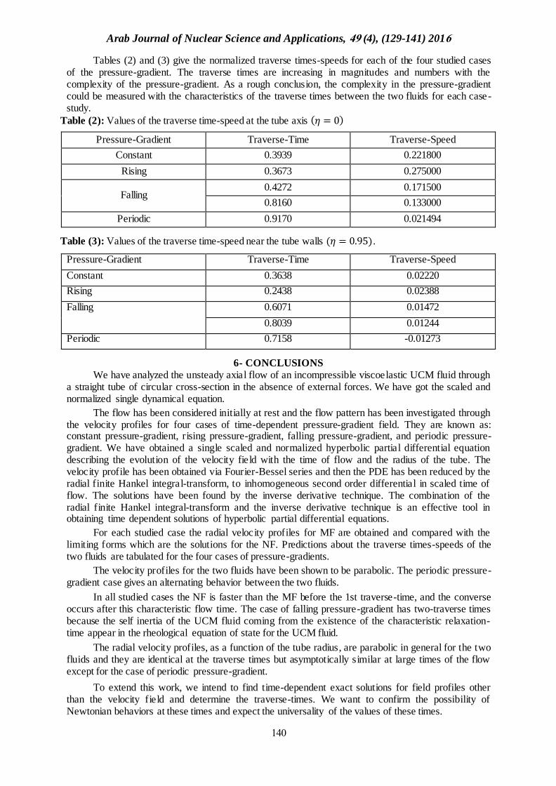
Tables (2) and (3) give the normalized traverse times-speeds for each of the four studied cases of the pressure-gradient. The traverse times are increasing in magnitudes and numbers with the complexity of the pressure-gradient. As a rough conclusion, the complexity in the pressure-gradient could be measured with the characteristics of the traverse times between the two fluids for each case-study.

Table (2): Values of the traverse time-speed at the tube axis (𝜂 = 0)

Pressure-Gradient Traverse-Time Traverse-Speed

Constant 0.3939 0.221800

Rising 0.3673 0.275000

Falling 0.4272 0.171500

0.8160 0.133000

Periodic 0.9170 0.021494

Table (3): Values of the traverse time-speed near the tube walls (𝜂 = 0.95).

Pressure-Gradient Traverse-Time Traverse-Speed

Constant 0.3638 0.02220

Rising 0.2438 0.02388

Falling 0.6071 0.01472

0.8039 0.01244

Periodic 0.7158 -0.01273

6- CONCLUSIONS

We have analyzed the unsteady axial flow of an incompressible viscoelastic UCM fluid through a straight tube of circular cross-section in the absence of external forces. We have got the scaled and normalized single dynamical equation.

The flow has been considered initially at rest and the flow pattern has been investigated through the velocity profiles for four cases of time-dependent pressure-gradient field. They are known as: constant pressure-gradient, rising pressure-gradient, falling pressure-gradient, and periodic pressure-gradient. We have obtained a single scaled and normalized hyperbolic partial differential equation describing the evolution of the velocity field with the time of flow and the radius of the tube. The velocity profile has been obtained via Fourier-Bessel series and then the PDE has been reduced by the radial finite Hankel integral-transform, to inhomogeneous second order differential in scaled time of flow. The solutions have been found by the inverse derivative technique. The combination of the radial finite Hankel integral-transform and the inverse derivative technique is an effective tool in obtaining time dependent solutions of hyperbolic partial differential equations.

For each studied case the radial velocity profiles for MF are obtained and compared with the limiting forms which are the solutions for the NF. Predictions about the traverse times-speeds of the two fluids are tabulated for the four cases of pressure-gradients.

The velocity profiles for the two fluids have been shown to be parabolic. The periodic pressure-gradient case gives an alternating behavior between the two fluids.

In all studied cases the NF is faster than the MF before the 1st traverse-time, and the converse occurs after this characteristic flow time. The case of falling pressure-gradient has two-traverse times because the self inertia of the UCM fluid coming from the existence of the characteristic relaxation-time appear in the rheological equation of state for the UCM fluid.

The radial velocity profiles, as a function of the tube radius, are parabolic in general for the two fluids and they are identical at the traverse times but asymptotically similar at large times of the flow except for the case of periodic pressure-gradient.

To extend this work, we intend to find time-dependent exact solutions for field profiles other than the velocity field and determine the traverse-times. We want to confirm the possibility of Newtonian behaviors at these times and expect the universality of the values of these times.


919

APPENDIX

To modify Eq. (22), Bessel’s differential equation is reformulated as,

(𝑑𝜂2 +

1

𝜂𝑑𝜂) 𝐽0

(𝜁𝑛𝜂) = −𝜁𝑛2𝐽0

(𝜁𝑛𝜂)

(52)

Hankel integral-transform is defined by,

𝐻0

{𝐽0(𝜁𝑛𝜂)} = ∫ 𝐽0

(𝜁𝑚𝜂)𝐽0(𝜁𝑛𝜂)𝜂 𝑑𝜂

1

0

(53)

where the ortho-normalization relations(26) of the Bessel function reads,

∫ 𝐽𝑖 (𝑆𝑚

𝑟

𝑎) 𝐽0 (𝑆𝑛

𝑟

𝑎) 𝑟𝑑𝑟

𝑎

0

= (𝑎2

2) 𝐽𝑖+1

2(𝑆𝑚)𝛿𝑚𝑛 for 𝑚, 𝑛 > −1,

(54)

𝐻0

{𝐽0(𝜁𝑛𝜂)} = (

1

2) 𝐽1

2(𝜁𝑚)𝛿𝑚𝑛 .

(55)

The indefinite integral involving Bessel function(28) will become,

∫ 𝐽0(𝑟)𝑟𝑑𝑟 = 𝑟 𝐽1

(𝑟), (56)

𝐻0

{1} = (1

𝜁𝑛

) 𝐽1(𝜁𝑛

). (57)

ACKNOWLEDGEMENT

The authors would like to express their gratitude to Prof. Dr. O. M. Osman, Department of

Physics, Cairo University, Giza 12613, Egypt, for his careful assessment and the fruitful comments and

suggestions regarding the whole research and the initial version of this work.

REFERENCES

(1) R. P. Chhabra and J. F. Richardson; Non-Newtonian Flow in the Process Industries: Fundamentals and

Engineering Applications, Butterworth Heinemann Publishers; 1–5 (1999).

(2) G. Radhakrishnamacharya, P. Chandra and M. R. Kaimal; Bulletin Math. Biol.; 43(2), 151–163 (1981).

(3) C. Kouris and J. Tsamopoulos; Chem. Eng. Sci.; 55, 5509–5530 (2000).

(4) M. G. Blyth, P. Hall and D. T. Papageorgiou; J. Fluid Mech.; 481, 187–213 (2003).

(5) G. K. Ramesh, Mahesha, B. J. Gireesha and C. S. Bagewadi; Acta Math. Univ. Comenianae; LXXX(2),

171–184 (2011).

(6) I. Siddique and S. Iftikhar; Appl. Math. Inf. Sci.; 6(3), 483–489 (2012).

(7) J. P. Pascal and H. Pascal; Int. J. Non-Linear Mech.; 30(4), 487–500 (1995).

(8) N. T. E. Dabe, G. M. Moatimid and H. S. M. Ali; Z. Naturforsch; 57a, 863–873 (2002).

(9) K. Avinash, J. A. Rao, Y. V. K. R. Kumar and S. Sreenadh; J. of Appl. Fluid Mech.; 6(1), 143–148 (2013).

(10) D. Tong, Xianmin Zhang and Xinhong Zhang; J. Non-Newton. Fluid Mech.; 156, 75–83 (2009).

(11) M. Kamran, M. Imran and M. Athar; Nonlinear Analysis: Modelling and Control; 15(4), 437–444 (2010).

(12) J. M.-Mardones and C. P.-Garcia; J. Phys.: Condens. Matter; 2(5), 1281–1290 (1990).

(13) M. Zidan; Rheol. Acta; 20(4), 324–333 (1981).

(14) Y. Yin and K.-Q. Zhu; Appl. Math. Comput.; 173, 231–242 (2006).

(15) H. Qi and H. Jin; Acta Mechanica Sinica; 22, 301–305 (2006).

(16) A. I. P. Miranda and P. J. Oliveira; Korea-Australia Rheol. J.; 22(1), 65–73 (2010).

(17) S. Wang, M. Zhao and X. Li; Cent. Eur. J. Phys.; 12(6), 445–451 (2014).

(18) S. L. Zhou and L. Hou;Advances in Pure Mathematics; 5, 233–239 (2015).

(19) E. Jiméneza, J. Escandóna, O. Bautista and F. Méndezb; J. Non-Newton. Fluid Mech.;227, 17–29 (2016).

(20) K. D. Rahaman and H. Ramkissoon; J. Non-Newton. Fluid Mech.; 57, 27–38 (1995).

(21) H. T. Banks, S. Hu and Z. R. Kenz; Adv. Appl. Math. Mech.; 3(1), 1–51 (2011).

(22) J. H. Spurk and N. Aksel; Fluid Mechanics second edition, Springer; 269–278 (2008).

(23) D. Terzopoulos and K. Fleiseher; Comput. Graph.; 22(4), 269–278 (1988).

(24) F. Olsson and J. Ystrom; J. Non-Newton. Fluid Mech.; 48, 125–145 (1993).

(25) D. M. Carvalho, M. F. Tome’, J. A. Cuminato, A. Castelo and V. G. Ferreira; TEMA Tend. Mat. Appl.

Comput.; 5(2), 195–204 (2004).

(26) G. B. Arfken and H. J.Weber; Mathematical Methods for Physicists sixth edition, Elsevier Inc.; 695, 694–

696 and 356 (2005).

(27) K. V. Zhukovsky; App. Math.; 2(2), 34–39 (2012).

(28) M. R. Spiegel, S. Lipschutz and J. Liu; Schaum’s Outline Series: Mathematical Handbook of Formulas

and Tables third edition, The McGraw-Hill Companies Inc.; 159 and 54 (2009).

(29) L. Ci-qtm and H. Jun-qi; Appl. Mathe. Mech. English edition; 10(II), 989–996 (1989).

(30) C. Fetecau, A. Mahmood and M. Jamil; Commun. Nonlinear Sci. Numer. Simulat.; 15, 3931–3938

(2010).

(31) P. Y. Huang and J. Feng; J. Non-Newtonian Fluid Mech.; 60, 179–198 (1995).

unsteady axial flows of upper-convected maxwell fluid in …15) 1 - 16.pdf · unsteady axial flows...

Documents