Unsecured Indebtedness in the United Kingdom — implicationsfrom a rational agent model∗

Justin van de Ven†and Martin Weale‡

Contents1 Introduction 5

2 Recent Trends in Personal Sector Indebtedness 72.1 Aggregate trends . . . . . . . . . . . . . . . . . . . . . . . . . . . . . . . . . . . . . . . . 72.2 Distributional data . . . . . . . . . . . . . . . . . . . . . . . . . . . . . . . . . . . . . . . 102.3 Summary . . . . . . . . . . . . . . . . . . . . . . . . . . . . . . . . . . . . . . . . . . . . 17

3 A Rational Agent Model of Consumption and Labour Supply 183.1 The utility function . . . . . . . . . . . . . . . . . . . . . . . . . . . . . . . . . . . . . . . 193.2 The wealth constraint . . . . . . . . . . . . . . . . . . . . . . . . . . . . . . . . . . . . . 203.3 The tax function . . . . . . . . . . . . . . . . . . . . . . . . . . . . . . . . . . . . . . . . 223.4 Household income dynamics . . . . . . . . . . . . . . . . . . . . . . . . . . . . . . . . . . 233.5 Modelling adults and children . . . . . . . . . . . . . . . . . . . . . . . . . . . . . . . . . 233.6 Model solution procedure . . . . . . . . . . . . . . . . . . . . . . . . . . . . . . . . . . . 273.7 Summary . . . . . . . . . . . . . . . . . . . . . . . . . . . . . . . . . . . . . . . . . . . . 29

4 Model Calibration 304.1 The data . . . . . . . . . . . . . . . . . . . . . . . . . . . . . . . . . . . . . . . . . . . . 324.2 Calibration of the income process . . . . . . . . . . . . . . . . . . . . . . . . . . . . . . . 334.3 Calibration of preference parameters . . . . . . . . . . . . . . . . . . . . . . . . . . . . . 344.4 The fit between simulated and sample age profiles . . . . . . . . . . . . . . . . . . . . . 354.5 Summary . . . . . . . . . . . . . . . . . . . . . . . . . . . . . . . . . . . . . . . . . . . . 43

5 Dis-aggregating Net Wealth to Identify Housing and Collateralised Debt 455.1 Summary . . . . . . . . . . . . . . . . . . . . . . . . . . . . . . . . . . . . . . . . . . . . 48

6 Intuition Behind the Life-cycle Model of Behaviour 48

7 Saving and Indebtedness in a Rational Agent Model 507.1 Behaviour a representative population cohort . . . . . . . . . . . . . . . . . . . . . . . . 507.2 Population subgroups distinguished by education . . . . . . . . . . . . . . . . . . . . . . 617.3 Housing and mortgage debt . . . . . . . . . . . . . . . . . . . . . . . . . . . . . . . . . . 657.4 Summary . . . . . . . . . . . . . . . . . . . . . . . . . . . . . . . . . . . . . . . . . . . . 67

8 The Incidence of Poverty and Over-Indebtedness 678.1 Some definitions . . . . . . . . . . . . . . . . . . . . . . . . . . . . . . . . . . . . . . . . 688.2 The characteristics that lead to over-indebtedness and poverty . . . . . . . . . . . . . . 698.3 The likelihood of becoming over-indebted when behaving rationally . . . . . . . . . . . . 758.4 Summary . . . . . . . . . . . . . . . . . . . . . . . . . . . . . . . . . . . . . . . . . . . . 80

∗Draft — Preliminary and Incomplete. Please do not quote without the prior permission of the authors.†NIESR. jvandeven@niesr.ac.uk‡NIESR. mweale@niesr.ac.uk

1

9 Summary and Conclusions 80

A Household level data for assets and debt from the British Household Panel Survey 88A.1 Housing wealth . . . . . . . . . . . . . . . . . . . . . . . . . . . . . . . . . . . . . . . . . 88A.2 Securities wealth . . . . . . . . . . . . . . . . . . . . . . . . . . . . . . . . . . . . . . . . 89A.3 Pension wealth . . . . . . . . . . . . . . . . . . . . . . . . . . . . . . . . . . . . . . . . . 89

B Simulated Tax and Benefits Policy 95

C Calibration Statistics for Education Specific Subgroups 95

D Additional Contour Maps of Over-Indebtedness and Poverty 95

List of Figures1 Historical Economic Indicators for the UK . . . . . . . . . . . . . . . . . . . . . . . . . . 92 Debt to Disposable Income Ratios for the UK . . . . . . . . . . . . . . . . . . . . . . . . 103 Debt Servicing and Debt to Assets Ratios for the UK . . . . . . . . . . . . . . . . . . . 114 Proportion of Population Net Debtors by Age — BHPS data for 2000/01 . . . . . . . . . 125 Average Net Wealth by Age Group and Wealth Quintile . . . . . . . . . . . . . . . . . . 146 Average Net Liquid Wealth by Age Group, Education, and Wealth Quintile . . . . . . . 157 Cumulative Proportion of Births by Household Age . . . . . . . . . . . . . . . . . . . . . 258 Timing of Retirement — simulated versus survey data . . . . . . . . . . . . . . . . . . . . 379 Private Non-Property Income Profiles by Age — simulated versus survey data . . . . . . 3810 Disposable Non-Property Income Profiles by Age — simulated versus survey data . . . . 3911 Consumption Profiles by Age — simulated versus survey data . . . . . . . . . . . . . . . 4012 Wealth Profiles by Age — simulated versus survey data . . . . . . . . . . . . . . . . . . . 4313 Proportion of Population Net Debtors by Age — simulated and sample data . . . . . . . 5314 Average Net Debt per Debtor (liquid wealth) — simulated and sample statistics . . . . . 5415 Life Profiles of Financial Statistics Generated by Model Calibrated to the Full UK Pop-

ulation . . . . . . . . . . . . . . . . . . . . . . . . . . . . . . . . . . . . . . . . . . . . . . 5816 Simulated Life Profiles of Demographic and Labour Statistics . . . . . . . . . . . . . . . 6017 Average Net Income of Simulated Households by Age and Education Level . . . . . . . 6218 Indebtedness by Age and Education — simulated data . . . . . . . . . . . . . . . . . . . 6319 Housing and Mortgage Statistics by Age — simulated and survey data . . . . . . . . . . 6620 Probability of Being Over-Indebted or Poor in at least One Year Between Ages 20 and

24 — contour maps by wage and wealth at age 20 . . . . . . . . . . . . . . . . . . . . . . 7021 Probability of Being Over-Indebted or Poor in at least One Year Between Ages 25 and

29 — contour maps by wage and wealth at age 25 . . . . . . . . . . . . . . . . . . . . . . 7222 Probability of Being Over-Indebted or Poor in at least One Year Between Ages 60 and

64 — contour maps by wage and wealth at age 60 . . . . . . . . . . . . . . . . . . . . . . 7423 Proportions of Population Over-Indebted / Credit Constrained by Age . . . . . . . . . . 7524 Probability of Single Adults Being Over-Indebted or Poor in at least One Year Between

Ages 25 and 29 — contour maps by wage and wealth at age 25 . . . . . . . . . . . . . . 7725 Probability of Couples Being Over-Indebted or Poor in at least One Year Between Ages

25 and 29 — contour maps by wage and wealth at age 25 . . . . . . . . . . . . . . . . . 7826 Life profiles of households constrained at age 30 . . . . . . . . . . . . . . . . . . . . . . . 8127 Wage Profiles by Age and Education . . . . . . . . . . . . . . . . . . . . . . . . . . . . . 9328 Simulated Tax Functions — Working Lifetime . . . . . . . . . . . . . . . . . . . . . . . . 9629 Tax Functions for Early and Later Retirement . . . . . . . . . . . . . . . . . . . . . . . 9730 Tax Functions for Retirement . . . . . . . . . . . . . . . . . . . . . . . . . . . . . . . . . 9831 Timing of Retirement — simulated versus survey data for lower educated households . . 9832 Private Non-Property Income Profiles by Age — simulated versus survey data for lower

educated households . . . . . . . . . . . . . . . . . . . . . . . . . . . . . . . . . . . . . . 9933 Disposable Non-Property Income Profiles by Age — simulated versus survey data for lower

educated households . . . . . . . . . . . . . . . . . . . . . . . . . . . . . . . . . . . . . . 100

2

34 Consumption Profiles by Age — simulated versus survey data for lower educated households10135 Timing of Retirement — simulated versus survey data for higher educated households . . 10236 Private Non-Property Income Profiles by Age — simulated versus survey data for higher

educated households . . . . . . . . . . . . . . . . . . . . . . . . . . . . . . . . . . . . . . 10337 Disposable Non-Property Income Profiles by Age — simulated versus survey data for

higher educated households . . . . . . . . . . . . . . . . . . . . . . . . . . . . . . . . . . 10438 Consumption Profiles by Age — simulated versus survey data for higher educated households10539 Probability of Being Over-Indebted or Poor in at least One Year Between Ages 34 and

39 — contour maps by wage and wealth at age 34 . . . . . . . . . . . . . . . . . . . . . . 10640 Probability of Being Over-Indebted or Poor in at least One Year Between Ages 34 and

39 — contour maps by wage and wealth at age 34 . . . . . . . . . . . . . . . . . . . . . . 107

List of Tables1 Statistical Correlations between Debt and Household Characteristics — BHPS survey data 172 Regression Statistics for Nested Logit Model of Household Size . . . . . . . . . . . . . . 263 Distribution of the Amount Owed by Debtors (Unsecured Debt) . . . . . . . . . . . . . 314 Calibrated Model Parameters for Representative Sample of UK Population . . . . . . . 365 Calibrated Model Parameters for Population Sub-samples Distinguished by Level of Ed-

ucation . . . . . . . . . . . . . . . . . . . . . . . . . . . . . . . . . . . . . . . . . . . . . 446 Regression Statistics for Equations Used to Simulate Housing . . . . . . . . . . . . . . . 477 Regression Statistics for Equations Used to Simulate Mortgages . . . . . . . . . . . . . . 488 Sample Selection Model of Weekly Wages . . . . . . . . . . . . . . . . . . . . . . . . . . 93

3

Summary

This report is the end of project submission for the Understanding Debt project undertaken by NIESR

for the DWP and DTI. The report focuses upon undertaking a rigorous analysis of private sector

indebtedness, and unsecured debt in particular. Key objectives include:

• to explore the interactions between saving and unsecured indebtedness that are derived from an

articulated and carefully calibrated rational agent model of the household,

• to consider the extent to which the current accumulation of debt can be explained as the productof rational responses to the prevailing economic environment,

• to explore the determinants and prevalence of over-indebtedness when individuals make sensiblefinancial decisions,

Key findings of the current report are:

• rational households take on unsecured debt when they expect incomes to rise in the future — inthis context debt is a positive mechanism allowing income smoothing over the lifecycle.

• the rational agent model substantially under-states both non-pension wealth and unsecured debtreported for the private sector in the National Accounts. Although it is conjectured that the

disparity for non-pension wealth could be resolved by including a bequest motive, best estimates

for the effects of adjustments to reconcile the levels of unsecured debt suggest that the model

would still understate the National Accounts aggregate by 30%.

• unsecured debt generated by the rational agent model tends to arise as the product of low incomes,which in turn are due to a marital dissolution or involuntary unemployment. These observations

are qualitatively consistent with survey data, and emphasise the importance of “indirect drivers”

of private sector indebtedness.

• the rational agent model suggests that the trend toward a higher educated population shouldresult in greater demand for credit early in any given birth cohort’s lifetime, and larger debts for

those who are indebted. If this result is valid, then it may provide a motive to expand the role of

student loan programmes.

• the rational agent model implies that approximately one fifth of all households should experienceat least one year of over-indebted and poverty during their lives. This result implies that over-

indebtedness and financial deprivation cannot simply be dismissed as a product of poor financial

planning.

4

1 Introduction

Unsecured indebtedness in the UK personal sector has risen sharply during the last half century, from

6.3% of GDP in 1950 to 17.7% of GDP — £234 billion — today (2007Q1).1 This trend, matched by

the experience of other G7 countries, has been the subject of growing public concern.2 Nevertheless,

it remains unclear whether current borrowing patterns should excite alarm. The trend toward higher

household debt may, for example, be a rational response to the favourable economic conditions that

have prevailed during recent decades, and the increasingly liberal terms of personal borrowing. This

report explores the interactions between household savings and indebtedness that are described by

a rational agent model, under the assumption that individuals are perfect financial planners. Given

credible assumptions regarding the economic environment, we also consider how closely the behaviour

generated by our rational agent model reflects the pattern of unsecured debt that is currently observed

in the UK.

The related literature

A large literature has tested the ability of the life-cycle framework to capture observed aspects of

consumer behaviour.3 Most of this literature has, however, ignored the specific effects of consumer

credit on consumption decisions by assuming either that individuals cannot borrow, or that they have

infinite available credit. In the former case, consumer credit is explicitly omitted, and in the latter debt

affects consumption only to the extent that it determines the lifetime resources that are available for

allocation. For debt to have a prominent influence on consumer behaviour under the life-cycle model,

borrowing must be rationed so that it is either subject to strict limits, or to higher interest rates than

those earned on financial assets.

Since the mid 1980’s, a great deal of work has been done to consider the influence of liquidity

constraints on consumption and savings behaviour in the context of uncertain future labour income.4

Simulation studies have suggested that liquidity constraints can affect the consumption behaviour of

individuals, even if they have a low probability of ever actually being constrained, and theoretical

advances mean that the underlying processes are now well understood.5 Furthermore, empirical analyses

1Solomou & Weale (1997) report that personal sector indebtedness in the UK was £2.175bn in 1950. Personal sectorunsecured indebtedness for 2006Q1 reported by the Office for National Statistics, ONS (calculated as the sum of codesNNRG, NNRK and NNRU). GDP in the UK was £13.162bn in 1950, and £1,319.485bn for the 12 months to 2007Q1, asreported by the ONS, code YBHA.

2See, for example, articles in the Financial Times, 28/07/2006 “Banks see rise in bad debts”, and the Daily Express,27/09/2006 “Brits ‘have worst debts in Europe’”. Similarly, in the Australian broadsheet, The Age, 12/11/2006, “Debthell for middle class”.

3 See Browning & Crossley (2001) for a review.4Carroll (2001), p.27, cites Zeldes (1984) as the first study in this field.5 See Zeldes (1989b) for an early example of simulation work, and Low (2005) for a contemporary example. Regarding

the theoretical underpinnings of precautionary savings motives, see Carroll & Kimball (1996) for behavioural responsesin the absence of liquidity constraints, Carroll & Kimball (2001) when households are not permitted to borrow, andFernandez-Corugedo (2002) when differential interest rates apply to savings and borrowing (so-called “soft constraints”).

5

suggest that liquidity constraints play an important role in determining consumer behaviour in practice

(e.g. Zeldes (1989a) and Gross & Souleles (2002) using US data, and Stephens (2006) and Benito &

Mumtaz (2006) for recent studies using UK data). Gross & Souleles (2002), for example, use a detailed

panel data set compiled by several different credit card providers in the US to determine the influence

of credit supply on consumption. They find that the average marginal propensity to consume out of

liquidity is strongly significant, ranging between 10 and 14 percent. They also find that the MPC is

higher for individuals who are close to their credit limit (consistent with a binding liquidity constraint),

and lower but significant for those starting well below their credit limit (consistent with a precautionary

savings motive).

Key objectives of the analysis

The primary purpose of the current study is to explore the interactions between saving and unsecured

indebtedness that are derived from an articulated and carefully calibrated structural model of the

household. The model is ‘articulated’ in the sense that a great deal of effort has been spent in obtaining

a reasonably detailed reflection of the characteristics that have been cited in survey data as key drivers

of unsecured indebtedness. It is a structural model in the sense that it is based upon an explicit

behavioural framework in which agents — households in the current study — are considered to make

their decisions regarding saving and labour supply to maximise expected lifetime utility, subject to the

various uncertainties that influence their future circumstances.

It is hoped that this analysis will help to inform policy makers regarding the motives that provide

potential explanations for patterns of behaviour toward unsecured indebtedness and saving more gener-

ally. Furthermore, by comparing the simulated behaviour against data regarding actual consumer credit

use, the study contributes to the substantial literature that tests whether the rational agent life-cycle

model provides an adequate representation of real-world behaviour, or in what ways it may be deficient.

Comparisons with survey data will also help to identify whether — given plausible assumptions regarding

the economic environment — contemporary consumer borrowing may be imprudent.

Analytical approach

Indebtedness bears upon the financial circumstances of individuals in three important respects. It is a

liability on the lifetime resources that are available for consumption, it draws individuals closer to any

period specific liquidity constraint that they may face, and it influences implicit rates of return to the

extent that it is used to finance investment. This study focuses primarily on unsecured indebtedness,

omitting incentives for financial leveraging. The current focus reflects the observation that repayment

difficulties (and hence liquidity constraints) are strongly associated with unsecured indebtedness, with

6

consequent implications for consumption and welfare.6

The stochastic dynamic programming model that is used to undertake the analysis has been carefully

designed to capture key factors that influence household indebtedness. Households are subject to

both hard and soft liquidity constraints, in the sense that the interest rate charged on debt is an

increasing function of a household’s debt to income ratio, and each household is subject to an age specific

credit limit. This specification implies that simulated households may experience a downward spiral

of increasing indebtedness and higher interest charges, which influences their precautionary savings

motive. Households are considered to make consumption and labour supply decisions to maximise

expected lifetime utility, subject to uncertainty regarding their labour income, marital status, number

of dependent children, and time of death. This model is calibrated to survey data, and is used to explore

the interaction between indebtedness, saving, and labour supply.

Outline of the report

Section 2 presents statistics that place current levels of household debt in their historical context, and

describes the contemporary distribution of indebtedness. Section 3 describes the structural dynamic

programming model that we use to analyse behaviour towards indebtedness, and Sections 4 and 5

report the model calibration. The paper has been structured so that the policy focussed reader may

omit the subsections of Section 3 (a review of the introductory discussion is encouraged), and Sections

4 and 5 without handicap. A brief review of the intuition behind the life-cycle model, as it relates

to household saving and indebtedness is provided in Section 6. Section 7 focuses upon describing

the behaviour toward saving and indebtedness implied by our rational agent model, and relating the

behaviour toward indebtedness to contemporary survey data. Implications of the model for the related

issues of over-indebtedness and poverty are explored in Section 8. A summary of results and associated

discussion are provided in a concluding section.

2 Recent Trends in Personal Sector Indebtedness

This section provides a brief review of statistical evidence regarding household indebtedness in the UK.

We begin by describing trends in aggregate data, before reporting distributional observations for a

contemporary population cross-section.

2.1 Aggregate trends

The period following the housing market crisis of the early 1990’s has been particularly favourable

for holding debt in the UK. Figure 1 displays five key statistics that place the current borrowing

6See, for example, Inflation Report, November 2006, Bank of England, p. 15.

7

environment in its historical context. The top panel of the figure reports quarterly data for income

growth and fluctuations in the unemployment rate observed since 1971Q1 (the earliest date for which

data are available). These data indicate that real disposable household income has grown reasonably

smoothly at a rate of 2.8% per annum during the last three and a half decades, and is now 2.7 times

what it was in 1971.7 At the same time, the unemployment data reveal a substantial degree of temporal

variation, peaking at values in excess of 10% during the recessions of the early 1980’s and early 1990’s,

between troughs that are as low as 3.4% (1973Q4). In this context, the last 10 years are notable for

the low and stable unemployment rates observed.

The bottom panel of Figure 1 reports 12 month moving averages for inflation, the base interest rate,

and interest rate volatility. The figure makes clear that all three of these statistics have exhibited a

downward trend during the past three decades, and have been relatively low and stable for the last

decade. Although the highs observed following the OPEC oil crisis may be taken as something of an

outlier, inflation, interest rates, and interest rate volatility were also substantially higher during the

recessions of the early 1980’s and 1990’s than they have been for the last 10 years.8

Strong income growth, low inflation, and low interest rates imply that debt is now more affordable

than it was in the past. Low unemployment, and low interest rate volatility imply that debt servicing

has been less risky. In this context, it is of little surprise that households have chosen to take on more

debt. The extent to which household indebtedness has grown is depicted in Figure 2, which reports

quarterly ratios of mortgage debt and unsecured credit to disposable income. These data reveal that

mortgage debt has grown particularly strongly over the 20 year period for which data are available — the

mortgage to disposable income ratio is now (2007Q1) just over twice what it was in 1987Q1. Although

the ratio of unsecured debt to disposable income has exhibited more variation than that for mortgages

(declining after the housing crisis of 1990), it has also exhibited strong growth, and is now more than

one and a half times what it was in 1993Q4. It is of note that both debt ratios are now higher than

they have been at any other time in the past 20 years.

Although the debt to income ratios reported in Figure 2 show substantial growth since 1987, the

favourable economic conditions have offset the associated impact on household budgets and balance

sheets. Figure 3 reports quarterly data for the mortgage debt to financial assets ratio, unsecured debt

to financial assets ratio, and the aggregate debt servicing ratio.9 The figure indicates that all three

7Code NRJR refers to population aggregates, and so tends to slightly overstate the growth of disposable incomemeasured on a per capita basis.

8The low and stable rates of inflation that have been observed during the last five years in the UK co-incide with the implementation of inflation targeting that began in 1992. See the Bank of England website(http://www.bankofengland.co.uk/monetarypolicy/history.htm) for details regarding the evolution of monetary policyin the UK.

9As Nickell (2004) notes, the rise in the value of household assets is predominantly due to an increase in financialassets, as the effects of the housing boom tend to cancel out from a population wide perspective.

8

0

50

100

150

200

250

300

1971 Q1 1976 Q1 1981 Q1 1986 Q1 1991 Q1 1996 Q1 2001 Q1 2006 Q1year

Hou

seho

ld In

com

e (1

971

= 10

0)

0

2

4

6

8

10

12

14

Une

mpl

oym

ent R

ate

real household disposable income (1971 = 100) (Left Axis) unemployment rate (Right Axis)

0

5

10

15

20

25

30

1976 01 1986 01 1996 01 2006 01year

per c

ent

0

0.5

1

1.5

2

2.5

3

3.5

4

4.5

per c

ent

RPI annual percentage changes (annual averages) (Left Axis) official Bank interest rate (Left Axis)

12 month standard deviation of official Bank interest rate (Right Axis)

12 month moving averages

S o u r c e : D a t a r e p o r t e d by th e O N S o r th e B an k o f E n g la n d

O N S c o d e s : R e a l h o u s e h o ld d is p o s a b le in c om e = N R JR , u n em p loym en t r a t e = 1 0 0 . ( 1 - M G R Z / M G SF ) , R e t a i l P r ic e s In d e x (R P I ) = C ZBH

B oE c o d e s : M on th ly ave r a g e o f offi c ia l B a n k o f E n g la n d in t e r e s t ra t e = IUM A BED R

R P I d a t a r e p o r t e d f r om 1 9 7 6 t o a l i g n to e a r l i e s t d a t e f o r w h ich offi c ia l B a n k in t e r e s t r a t e ava i la b l e

Figure 1: Historical Economic Indicators for the UK

9

0.7

0.8

0.9

1

1.1

1.2

1.3

1.4

1.5

1.6

1987 Q1 1989 Q1 1991 Q1 1993 Q1 1995 Q1 1997 Q1 1999 Q1 2001 Q1 2003 Q1 2005 Q1 2007 Q1year

0.2

0.22

0.24

0.26

0.28

0.3

0.32

0.34

ratio of mortgage debt to disposable non-property income (Left Axis) ratio of unsecured debt to disposable non-property income (Right Axis)

S o u r c e : A l l d a t a r e p o r t e d by th e Offi c e fo r N a t io n a l S t a t i s t ic s

O N S c o d e s : M o r t g a g e d e b t = NN RQ + N NRR + NNR S , u n s e c u r e d d e b t = N NRG + NNRK + NNRU

D is p o s a b le n o n -p r o p e r ty in c om e = R PQ K - ROY L + ROYT - N R JN + ROYH

Figure 2: Debt to Disposable Income Ratios for the UK

statistics fell from peaks observed in 1990Q3, with only the ratio of mortgage debt to financial assets

now greater than the value it was then. Furthermore, responses to qualitative surveys suggest that

people now find their debts less burdensome than in the past.10 These statistics consequently suggest

that, in spite of the well publicised rise in private sector debt, the financial well-being of households

does not appear to have deteriorated substantially during the past decade.

2.2 Distributional data

Analysis of the distribution of debt amongst the UK population is complicated by the scarcity of

associated micro data. At the time of writing, the richest source of micro data regarding the assets and

debts held by UK households is the 2000/01 wave of the British Household Panel Survey (BHPS).11 This

survey reports the responses of just under 7000 households to a suite of questions that were designed

to identify household assets and liabilities. The cross-sectional wealth data from the 2000/01 wave of

the BHPS do not describe the practical experience of any population cohort. It is also well recognised

10See, for example, Over-indebtedness in Britain: a DTI report on the MORI financial services survey, 2004, see:http://www.dti.gov.uk/files/file18550.pdf.11 See Appendix A for further details regarding the BHPS. There are currently four main sources of wealth data for the

UK; the General Household Survey (primarily for housing wealth), the Family Resources Survey, the English LongitudinalStudy of Ageing (for the English population over the age of 50), and the BHPS. Following a review of these alternativedata sets, the BHPS was identified as the most comprehensive source of wealth data currently available for the UK.The wealth data provided by the BHPS are due to be updated in 2007 with the release of the 15th wave of the panel.The distribution of household assets and liabilities in the UK will also be greatly enhanced when the Wealth and Assetssurvey is made available, early results of which are scheduled to be released in December 2007, with the main report tobe released in Spring of 2009.

10

0.02

0.04

0.06

0.08

0.1

0.12

0.14

0.16

1987 Q1 1989 Q1 1991 Q1 1993 Q1 1995 Q1 1997 Q1 1999 Q1 2001 Q1 2003 Q1 2005 Q1 2007 Q1

year

0.1

0.12

0.14

0.16

0.18

0.2

0.22

0.24

0.26

0.28

0.3

aggregate debt servicing ratio (Left Axis) unsecured debt to financial assets (Left Axis) mortgage debt to financial assets (Right Axis)

S o u rc e : D a t a r e p o r t e d b y th e O N S o r th e B an k o f E n g la n d

O N S c o d e s : M o r tg a g e d e b t = NN RQ + N NRR + NNR S , u n s e c u r e d d eb t = N NRG + NNRK + NNRU , fi n a n c ia l a s s e t s = N NM L

B oE c o d e s : D eb t s e r v i c in g r a t io — u n p u b l i s h e d c a l c u la t io n s by th e B a n k o f E n g la n d

Figure 3: Debt Servicing and Debt to Assets Ratios for the UK

that the incidence of debt is commonly understated by surveys of this type, an issue that is discussed

at greater length in Section 7. Nevertheless, the associated distributional statistics, which are reported

here, provide a useful backdrop against which to interpret the behaviour generated by our rational agent

model.

Three measures of household wealth were imputed from the BHPS data: securities wealth, housing

wealth, and pension wealth.12 Although all three measures of wealth contribute to the aggregate

resources available to a household, differences in liquidity associated with each imply that they feature

differently in the household budget constraint. For the simulations that are presented in Section 7, we

distinguish between housing and securities wealth on the one hand, and pension wealth on the other.

This distinction reflects the observation that, in practice, borrowers can use remortgaging to finance

current consumption out of housing wealth, whereas it is not possible to leverage against pension wealth

during the working lifetime.13 The same distinction is consequently also used to frame the discussion

that is presented here. Housing and securities wealth is hereafter referred to as liquid wealth, and liquid

wealth together with pension wealth is referred to as total wealth.

12Wave 10 of the BHPS asked survey respondents for their personal estimates regarding the value of any residentialproperty that they owned, the value of associated mortgages, the value of their financial investment products, and the valueof any loan products. Pension wealth is highly opaque in the UK, and the BHPS did not include questions regarding thevalue of private pensions. Pension wealth was consequently imputed from the panel data provided by the BHPS followingthe approach described by Blundell et al. (2002). See the Appendix for full details.13 See Benito (2007) for recent UK evidence that households use housing equity to smooth over adverse economic shocks.

11

0

0.1

0.2

0.3

0.4

0.5

0.6

20 25 30 35 40 45 50 55 60 65

age

prop

. of p

opul

atio

n

liquid w ealth aggregate w ealth

S o u r c e : a u th o r c a lc u la t io n s u s in g (w e ig h t e d ) B H P S su rv e y d a t a

l iq u id w ea lt h e q u a l t o va lu e o f fi n a n c ia l s e c u r i t i e s p lu s r e s id e n t ia l p r o p e r ty

a g g r e g a t e w e a lt h e q u a l t o l iq u id w ea lt h p lu s va lu e o f p r iva t e ( p e r s o n a l a n d o c c u p a t io n a l ) p e n s io n s

Figure 4: Proportion of Population Net Debtors by Age — BHPS data for 2000/01

Figure 4 reports the proportion of households, by age and wealth specification, that were identified

by the BHPS survey data as net debtors. This figure indicates that, if imputed pensions are taken into

consideration, then very few households were identified as net debtors after age 25 in 2000/01.14 This

view, however, fails to reflect the short-term financial reality of most households. The second series

displayed in the figure reveals that a substantial proportion of the population possess negative net liquid

wealth, falling from a peak of more than half the population at age 20, to 10% by age 39, and then

gradually falling with age so that negligible households are identified as net debtors by age 6515. This

suggests that a substantial proportion of the working aged population make use of credit, particularly

when young.

To describe the size and distribution of the debts that were reported by households in the BHPS, and

how these relate to assets in the survey, Figure 5 displays the average net wealth of households, by age

group and wealth quintile. The two panels of the figure relate closely to the statistics that are reported

in Figure 4. Taking, for example, the lowest age band reported in Panel A of Figure 5, households in

the bottom two wealth quintiles have debts that exceed their liquid assets, while households in the third

quintile have debts that are approximately equivalent to their liquid assets. This is consistent with the

statistics displayed in Figure 4, which indicate that 40 to 50 percent of households between ages 20 and

14Less than 2.5% of households between ages 25 and 65 are identified as possessing total assets of lower value than theirtotal debts.15 0.27 percent

12

24 are debtors, measured with regard to net liquid wealth.

The statistics reported in Panel A of Figure 5 indicate that the net debts described by the BHPS

data are distributed highly unequally, with the vast majority of net debt held by the lowest population

quintile. In both panels of the figure, average net assets tend to rise with age, and only the lowest

population quintile holds negative liquid assets on average throughout most of the lifetime considered

in the figure. Nevertheless, the average net debt (based on liquid assets) of the lowest population

quintile falls by more than 40% from ages 20-24 to 25-29, and then by 40% again to ages 30-34. Hence,

net debt appears to be heavily concentrated in the poorest fifth of young households.

Perhaps more conspicuous in Figure 5 is the disparity with which household wealth is distributed.

The average net liquid wealth of the highest population quintile is approximately twice that of the next

most wealthy quintile for most of the age groups reported in the figure, for measures of both liquid

and total net wealth. Hence, the distribution of net wealth is skewed to the left, with few households

characterised as net debtors, the second to fourth population quintiles bunched relatively tightly, and

the most wealthy 20 percent of households holding a substantially disproportionate share of net wealth.

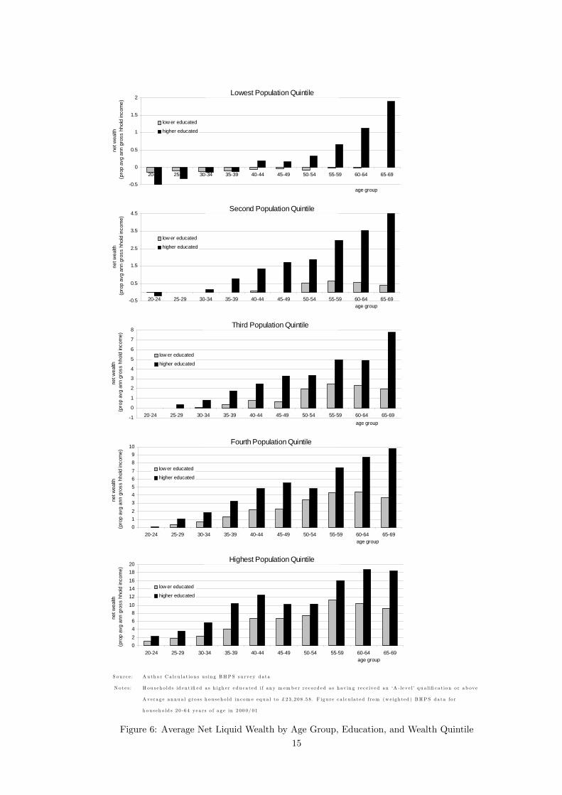
To obtain further detail regarding the distribution of debt amongst UK households, Figure 6 distin-

guishes the population with regard to whether any household member was recorded as having received

an ‘A-level’ qualification or higher, which split the full sample into two roughly equal halves.16 The

statistics reported in Figure 6 paint an interesting picture: although higher educated households are

wealthier on average, the largest net debts tend to be held by young households that are higher edu-

cated. Notably, these observations are consistent with the life-cycle hypothesis, which states that more

pronounced borrowing should be observed amongst households with expectations of higher income in

the future.

In addition to the statistics that are reported here, a number of recent studies have been conducted

to describe the characteristics of UK households that tend to incur substantial debts. Bridges & Disney

(2004), for example, use data from the Survey of Low Income Families to find that families with low

incomes tend to incur more substantial arrears. They also find that arrears are positively correlated

with the number of dependent children in a household, and negatively correlated with the age of the

reference person (consistent with the statistics reported above). Similar observations were found by

a Department of Trade and Industry report based upon the MORI Financial Services survey from

2004.17 Kempson (2002) reports, using qualitative data from 1647 householders across Britain in 2002,

that half of all households in financial difficulty attributed their problems to a loss of income, 15 percent

to low income, and 10 percent to each of over-commitment, relationship break-down, and unanticipated

16 41% of households were identified as having at least one individual with an A-level qualification or higher.17Over-indebtedness in Britain, op cit. In that report, individuals with low incomes, those with children and those in

their 20s and 30s were found to be more commonly over-indebted than the population average.

13

-2

0

2

4

6

8

10

12

14

20-24 25-29 30-34 35-39 40-44 45-49 50-54 55-59 60-64 65-69

low est quintile second quintile third quintile fourth quintile highest quintile

net w

ealth

as

a p

ropo

rtion

of a

vera

ge a

nnua

l gro

ss h

ouse

hold

inco

me

age band

Panel A: liquid wealth

-0.5

4.5

9.5

14.5

19.5

24.5

29.5

20-24 25-29 30-34 35-39 40-44 45-49 50-54 55-59 60-64 65-69

low est quintile second quintile third quintile fourth quintile highest quintile

net w

ealth

as

a p

ropo

rtion

of a

vera

ge a

nnua

l gro

ss h

ouse

hold

inco

me

age band

Panel B: total wealthSo u r c e : A u th o r C a lc u la t io n s u s in g B H P S su rve y d a t a

A ve r a g e a n nu a l g r o s s h o u s e h o ld in c om e e q u a l t o £ 2 3 ,2 0 8 .5 8 . F ig u r e c a l c u la t e d f r om

(w e ig h t e d ) B H P S d a t a f o r h o u s e h o ld s 2 0 -6 4 ye a r s o f a g e in 2 0 0 0 / 0 1

Figure 5: Average Net Wealth by Age Group and Wealth Quintile

14

-0.5

0

0.5

1

1.5

2

20-24 25-29 30-34 35-39 40-44 45-49 50-54 55-59 60-64 65-69

low er educated

higher educated

net w

ealth

(p

rop

avg

ann

gros

s hh

old

inco

me)

age group

Lowest Population Quintile

-0.5

0.5

1.5

2.5

3.5

4.5

20-24 25-29 30-34 35-39 40-44 45-49 50-54 55-59 60-64 65-69

low er educated

higher educated

net w

ealth

(p

rop

avg

ann

gros

s hh

old

inco

me)

age group

Second Population Quintile

-1

0

1

2

3

4

5

6

7

8

20-24 25-29 30-34 35-39 40-44 45-49 50-54 55-59 60-64 65-69

low er educated

higher educated

net w

ealth

(p

rop

avg

ann

gros

s hh

old

inco

me)

age group

Third Population Quintile

0123456789

10

20-24 25-29 30-34 35-39 40-44 45-49 50-54 55-59 60-64 65-69

low er educated

higher educated

net w

ealth

(p

rop

avg

ann

gros

s hh

old

inco

me)

age group

Fourth Population Quintile

02468

101214161820

20-24 25-29 30-34 35-39 40-44 45-49 50-54 55-59 60-64 65-69

low er educated

higher educated

net w

ealth

(p

rop

avg

ann

gros

s hh

old

inco

me)

age group

Highest Population Quintile

S o u r c e : A u th o r C a lc u la t io n s u s in g B H P S su rve y d a t a

N o t e s : H o u s e h o ld s id e n t ifi e d a s h ig h e r e d u c a t e d i f a n y m em b e r r e c o rd e d a s h av in g r e c e iv e d a n ‘A - le v e l ’ q u a l ifi c a t io n o r a b ov e

A ve r a g e a n nu a l g r o s s h o u s e h o ld in c om e e q u a l t o £ 2 3 ,2 0 8 .5 8 . F ig u r e c a lc u la t e d f r om (w e ig h t e d ) B H P S d a t a f o r

h o u s e h o ld s 2 0 -6 4 ye a r s o f a g e in 2 0 0 0 / 0 1

Figure 6: Average Net Liquid Wealth by Age Group, Education, and Wealth Quintile

15

expenses. For young people, low income was the main reason given for financial difficulties (accounting

for 25 percent), followed by loss of income (23 percent), and over-commitment (14 percent).

Table 1 reports statistics for two regression models of household debt (based on liquid wealth)

calculated using the BHPS survey data that are discussed above: a probit model, which describes the

probability that a household is indebted given the various characteristics reported in the table; and a

Tobit model, which indicates the magnitude of the associated debts.18 The probit regression coefficients

on age indicate that the probability of being indebted is particularly high between ages 20 and 30, and

to a lesser extent between ages 30 and 40, after which the probability falls away strongly. Similarly,

the Tobit model indicates that the size of debts held also falls strongly with age19 , following a period

of variation between ages 20 and 40. These observations are clearly consistent with the distributional

statistics discussed above.

Couples and divorcees have both a higher probability of being indebted, and larger debts, than

do otherwise similar single adults. In the case of couples, this may reflect access to credit and/or

expectations regarding future income prospects. In the case of divorce, it reflects the disruption that

accompanies relationship breakdown, and is consistent with the findings reported by Kempson (2002)

discussed above. In contrast to the various studies referred to above, however, the estimated statistics

reported in Table 1 imply that households with dependent children tend to have a lower probability of

being indebted, and are correlated with lower net debts. The differences between the statistics reported

here and the previously mentioned studies are most likely attributable to the current focus upon net

debt rather than arrears, and the fact that our sample is approximately nationally representative.20

All else being equal, education to A-level or above increases both the probability of being indebted,

and the likely net debt if indebted, consistent with the statistics reported in Figure 6. The level of

gross household income is associated with less pronounced indebtedness, whereas increases in income

over the immediately preceding 12 month period are associated with higher indebtedness. Although

this last observation may appear to contradict the associated findings reported by the studies that are

referred to above, it is important to take expectations regarding future income into account. If an

increase in income is considered to be transitory, then the life-cycle hypothesis implies that households

should save some of the wind-fall gain to finance higher consumption in the future. This would imply

18The equations considered here were arrived at after experimenting with various alternatives. The estimated coefficientsof the probit equation are not, in themselves, measures of probability. Nevertheless there is a positive association betweenthe probit coefficients and the likelihood of a positive observation (e.g. an individual being indebted). Details regardinghow probit coefficients translate into measures of probability are provided in any intermediate econometrics text book.See, for example, Johnston & DiNardo (1997), section 13.4.19 the Tobit regression is based upon an endogenous variable, where higher positive values indicate larger debts, and

households with positive net assets are censored to zero.20The possibility that the differences between the estimated effects of children on household indebtedness that are

reported here, and those of the studies referred to above are attributable to omitted variable bias is unlikely, giventhat the estimates reported in Table 1 are robust to the alternative specifications that were explored. Importantly, thealternative specifications that were considered include employment identifiers, and a distinction between labour and non-labour income. These are omitted from the table because the associated regression coefficients were highly insignificant.

16

Table 1: Statistical Correlations between Debt and Household Characteristics — BHPS survey data

Probit Model Tobit ModelVariable coefficient std error coefficient std errorAge

20-24 0.17327 0.09641 -5959.29* 1925.5425-29 0.12630 0.09520 -5150.32* 1937.5630-34 0.02596 0.09641 -8540.21* 1988.3235-39 0.03417 0.09881 -6805.88* 2030.7140-44 -0.32548* 0.11042 -12047.40* 2289.5145-49 -0.40931* 0.11554 -15655.60* 2426.1050-54 -0.67024* 0.12325 -20342.10* 2625.2955-59 -0.52917* 0.11621 -19326.70* 2476.6560-64 -1.09780* 0.13609 -28590.40* 2979.8065 and over -1.77536* 0.08420 -40064.70* 2083.99

Demographic Statussingle parent -0.01548 0.08813 -1795.74 1799.41couple without children 0.38751* 0.07577 7130.05* 1562.04couple with children 0.28779* 0.07902 3871.04* 1617.39divorced 0.23240* 0.07732 3411.59* 1605.45

Education A-level or higher 9.04E-04 4.57E-03 2450.53* 1168.35Gross household income -4.64E-06* 2.66E-06 -0.16381* 0.0573912 month change in income 3.07E-06 2.40E-06 0.09588 0.05088House ownership -1.73288* 0.06462 -27214.80* 1479.94

Log likelihood -1567.94 -10879.1Observations 6260 6260Correct predictions (%) 87.939Sigma** 22062.80* 554.746* estimate statistically significant at 95% confidence interval** estimated standard deviation of residualsAuthor calculations using data from waves 9 and 10 of the BHPSDebt measured with regard to liquid wealth

a negative correlation between an income change and debt, consistent with the observations made by

studies that explore the underlying reasons for over-indebtedness (including those discussed above). In

contrast, if an increase in income is considered to indicate a larger increase in income in the future, then

the life-cycle hypothesis will imply a positive correlation between income change and indebtedness, as

observed here. This effect will be exaggerated when an increase in income also provides greater access to

credit. Finally, the estimated statistics reported for house ownership in Table 1 indicate that residential

property reduces both the probability of being indebted, and the size of net debts, consistent with the

findings of earlier studies.

2.3 Summary

• Household sector indebtedness — both in absolute terms and relative to disposable income — hasincreased substantially during the last decade.

• The increased indebtedness of the household sector appears to be sustainable in context of theprevailing benign economic environment

• Household indebtedness appears to be heavily concentrated in the poorest fifth of young house-

17

holds (aged 30 and under). This has the advantage that young households have most of their

working lives ahead of them, and have a longer period over which to repay the debt.

• Young individuals who are higher educated tend to be more heavily indebted than otherwisesimilar lower educated individuals. This has the advantage that higher educated individuals can

be anticipated to be better able to afford the financial burden in the future.

• The rosy economic picture painted by population aggregate statistics masks severe financial hard-ship experienced by a minority of households who have experienced negative shocks to their

circumstances, as in the case of employment disruption or divorce.

We now describe the rational agent model that is used to explore behaviour toward savings and

indebtedness of heterogeneous agents during the life-course.

3 A Rational Agent Model of Consumption and Labour Supply

The decision unit in the model is the household. Households are considered to be fully described by

ten characteristics:

age - education - number of adults - number of children - private pensionswage rate - labour supply - consumption - net liquid wealth - time of death

The model is designed to consider household behaviour from age 20 to the maximum terminal age

of 110, disaggregated into annual increments. Households choose their consumption and labour supply

to maximise their expected lifetime utility, given their existing circumstances, preferences, and beliefs

regarding the future. A household’s circumstances are described by their age, education, number of

adults, number of children, wage rate, net liquid (non-pension) wealth, private pension rights, and time

of death. Preferences are defined by a utility function (that is the same for all households), and beliefs

are rational in the sense that they reflect the processes that generate household circumstances.

Care has been taken in specifying the model to capture factors that are important in determining the

financial welfare of households and their use of debt. The preceding section indicates that age, education,

and the treatment of pension wealth have an important bearing on the extent of indebtedness that is

identified by survey data for the population. Furthermore, incorporating an appreciation of uncertainty

into individual expectations regarding future circumstances dramatically increases the complexity of the

utility maximisation problem. As noted in the preceding section, the most prevalent causes given for

financial hardship are the loss of income, low income / over commitment, relationship breakdown, and

unanticipated expenses. Hence, of the eight characteristics that define the circumstances of a household,

four are considered to be stochastic (labour income, relationship status, number of children, and time

18

of death), and four are considered to be deterministic (age, education, private pensions and net liquid

wealth).

In the terminology of the dynamic programming literature, consumption and labour supply are

control variables that are considered to be selected to maximise the value function described by a

time separable utility function, subject to eight state variables, four of which are stochastic, and four

deterministic. Disaggregation of liquid wealth into housing and non-housing wealth, and identifying

collateralised debt, are undertaken outside of the formal dynamic programming problem.

Outline

This section begins by defining the assumed preference relation, before describing the wealth constraint,

the processes assumed for the evolution of income and household size, and concludes with an explanation

of the approach adopted to solve the lifetime utility maximisation problem. Calibration of the model

is reported in Section 4, and the methods adopted to simulate housing wealth and collateralised debt

are described in Section 5. The non-technical reader may skip directly to the discussion of the intuition

behind the life-cycle model provided in Section 6 without excessive handicap.

3.1 The utility function

Expected lifetime utility of household i at age t is described by the time separable function:

Ui,t =1

(1− 1/γ)Et110Xj=t

u

µci,jθi,j

, li,j

¶1−1/γδj−tφj−t,t (1)

where γ > 0 is the intertemporal elasticity of substitution (of total expenditure), Et is the expectations

operator, ci,t ∈ R+ is composite nondurable consumption, li,t ∈ {lW,na, 1} is the proportion of householdtime spent in leisure, and θi,t ∈ R+ is adult equivalent size based upon the McClements’ scale.21 Fromage 65, the household is forced to retire if it has not already chosen to do so, in which case li,t = 1 for

all t ≥ tSPA = 65.The labour supply decision is considered to be made between discrete alternatives, in response to

the view that this provides a closer reflection of reality than one in which labour supply is a continuous

choice variable for given wage rates.22 It also reflects the current focus on household indebtedness, and21See McClements (1977) on the McClements’ equivalence scale, and Balcer & Sadka (1986) and Muellbauer & van de

Ven (2004) on the use of this form of adjustment for household size in the utility function.22Although working time arrangements have become increasingly flexible since the 1970s, substantial labour market

rigidities continue to affect employment decisions. Fagan (2003), for example, reports that approximately 1 in 5 employedpeople in Europe work full-time when they would prefer to work part-time. The reasons most commonly given for themis-match include the perception that it would not be possible to do a desired job part-time, that part-time employment isnot offered by a desired employer, and that it would damage career prospects. Furthermore, cross-sectional data from the2002/03 Family Resources Survey indicate that approximately 80 percent of household income is earned by the householdreference person between ages 20 and 65 — a proportion that is approximately stable after age 27. The correlation betweenthe proportion of household reference people employed full-time by age, and the proportion participating in the labourforce is 0.971 between ages 20 and 65, and 0.978 for the population more generally. Higher correlations are observedbetween ages 55 and 64. The issue of heterogeneity of employment decisions is further complicated in the current contextby the considered policy environment (which tends to discourage part-time employment in later life due to the influenceof means tested benefits).

19

our view that this is influenced more by the extensive than the intensive labour margin. It should be

noted, however, that the assumption of a dichotomous labour supply decision is likely to dampen the

responsiveness of labour supply behaviour implied by the simulation model. Calibration of the model

is consequently likely to require a labour elasticity that overstates the practical reality. Furthermore,

omitting heterogeneity in the labour supply decision is likely to imply that the calibrated income process

will involve more variation than applies in practice.

The McClements’ scale depends upon the numbers of adults, nai,t, and children, nci,t in a household,

and its inclusion in the preference relation reflects the fact that household size has been found to have

an important influence on the timing of consumption (e.g. Attanasio & Weber (1995) and Blundell

et al. (1994)).23 φj−t,t is the probability of living to age j, given survival to age t, and δ is the discount

factor, which is assumed to be the same for all households and time invariant.24

A Constant Elasticity of Substitution function was selected for within period utility,

u

µci,jθi,j

, li,t

¶=

õci,jθi,j

¶(1−1/ε)+ α1/εl

(1−1/ε)i,t

! 11−1/ε

(2)

where ε > 0 is the (period specific) elasticity of substitution between equivalised consumption (ci,t/θi,t)

and leisure (li,t). The constant α > 0 is referred to as the utility price of leisure. The specification

of intertemporal preferences described by equations (1) and (2) is standard in the literature, despite

the contention associated with the assumption of time separability (see Deaton & Muellbauer (1980),

pp. 124-125, or Hicks (1939), p. 261). The specification of equation (2) implicitly assumes that

characteristics which affect utility, but are not explicitly stated, enter the utility function in an additive

way.

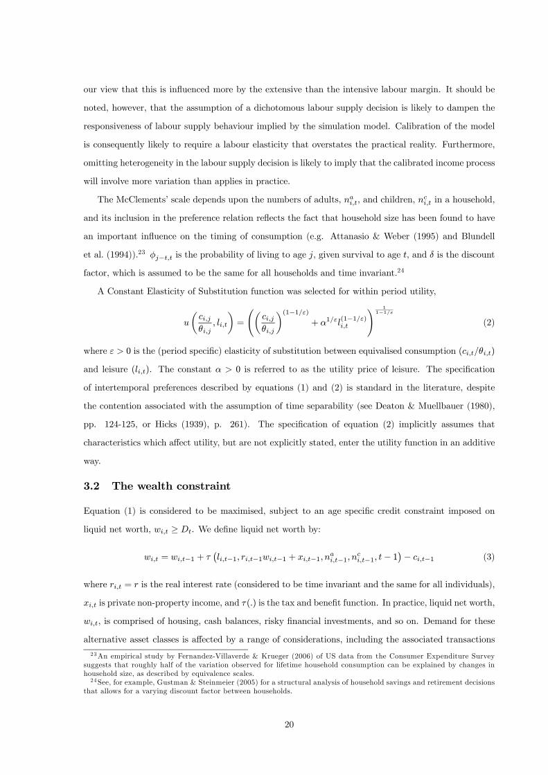
3.2 The wealth constraint

Equation (1) is considered to be maximised, subject to an age specific credit constraint imposed on

liquid net worth, wi,t ≥ Dt. We define liquid net worth by:

wi,t = wi,t−1 + τ¡li,t−1, ri,t−1wi,t−1 + xi,t−1, nai,t−1, n

ci,t−1, t− 1

¢− ci,t−1 (3)

where ri,t = r is the real interest rate (considered to be time invariant and the same for all individuals),

xi,t is private non-property income, and τ(.) is the tax and benefit function. In practice, liquid net worth,

wi,t, is comprised of housing, cash balances, risky financial investments, and so on. Demand for these

alternative asset classes is affected by a range of considerations, including the associated transactions

23An empirical study by Fernandez-Villaverde & Krueger (2006) of US data from the Consumer Expenditure Surveysuggests that roughly half of the variation observed for lifetime household consumption can be explained by changes inhousehold size, as described by equivalence scales.24 See, for example, Gustman & Steinmeier (2005) for a structural analysis of household savings and retirement decisions

that allows for a varying discount factor between households.

20

costs, the uncertainty of investment returns, differential tax treatment, and the consumption of housing

services. We simplify the analysis by abstracting from the asset allocation problem, and leave associated

sensitivity analysis as an issue for further research.

The function τ is a stylised representation of the UK tax and benefit system, and is described in

detail in subsection 3.3. During the working lifetime, t < tSPA, xi,t defines household labour income,

equal to the wage rate hi,t multiplied by a random factor ϕi,t if the household chooses to work, and zero

otherwise. The random factor is a dummy variable that identifies when a household receives a wage

offer (and thereby controls for involuntary unemployment). Importantly, the probability of a low wage

offer is considered to depend only upon marital status and is independent of age, so that the profile of

rates of employment is shaped by preferences and rates of pay, rather than by the exogenously defined

probability of a low wage offer. The household wage, hi,t, is considered to evolve following a stochastic

process that is described in subsection 3.4.

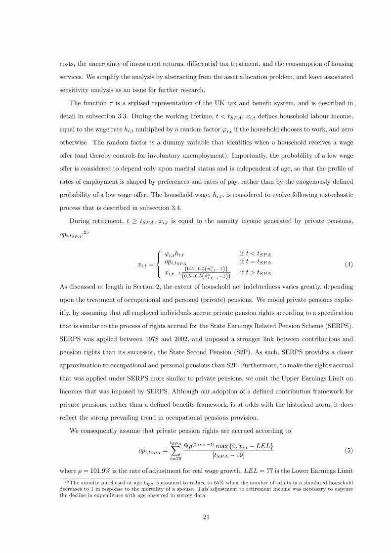
During retirement, t ≥ tSPA, xi,t is equal to the annuity income generated by private pensions,

opi,tSPA :25

xi,t =

⎧⎪⎨⎪⎩ϕi,thi,t if t < tSPAopi,tSPA if t = tSPA

xi,t−1(0.5+0.5(nai,t−1))(0.5+0.5(nai,t−1−1))

if t > tSPA(4)

As discussed at length in Section 2, the extent of household net indebtedness varies greatly, depending

upon the treatment of occupational and personal (private) pensions. We model private pensions explic-

itly, by assuming that all employed individuals accrue private pension rights according to a specification

that is similar to the process of rights accrual for the State Earnings Related Pension Scheme (SERPS).

SERPS was applied between 1978 and 2002, and imposed a stronger link between contributions and

pension rights than its successor, the State Second Pension (S2P). As such, SERPS provides a closer

approximation to occupational and personal pensions than S2P. Furthermore, to make the rights accrual

that was applied under SERPS more similar to private pensions, we omit the Upper Earnings Limit on

incomes that was imposed by SERPS. Although our adoption of a defined contribution framework for

private pensions, rather than a defined benefits framework, is at odds with the historical norm, it does

reflect the strong prevailing trend in occupational pensions provision.

We consequently assume that private pension rights are accrued according to:

opi,tSPA =

tSPAXt=20

Ψρ(tSPA−t)max {0, xi,t − LEL}[tSPA − 19] (5)

where ρ = 101.9% is the rate of adjustment for real wage growth, LEL = 77 is the Lower Earnings Limit

25The annuity purchased at age tspa is assumed to reduce to 65% when the number of adults in a simulated householddecreases to 1 in response to the mortality of a spouse. This adjustment to retirement income was necessary to capturethe decline in expenditure with age observed in survey data.

21

as applied in 2003, and Ψ = 0.25 is the accrual rate that was applied by SERPS for the 1978/79-1987/88

tax years (the most generous rate applied by the scheme).26

The interest rate is assumed to depend upon whether wi,t indicates net investment assets, or net

debts:

ri,t =

(rI if wi,t > 0

rDl +¡rDu − rDl

¢min

n −wi,tmax[xi,t,0.7hi,t]

, 1o, rDl < r

Du if wi,t ≤ 0

This specification for the interest rate implies that the interest charge on debt increases from a minimum

of rDl when the debt to income ratio is low, up to a maximum rate of rDu , when the ratio is high. The

specification also means that households in debt are treated more generously if they are working than

if they are not. The assumption that the maximum rate of interest is charged when net debt is equal

to or greater than the household full-time employment wage reflects the observation that less than 1

percent of households recorded by the 2000/01 BHPS with some labour income had unsecured debt

that exceeded their annual gross labour income.

3.3 The tax function

The function τ is a stylised representation of the UK tax and benefits system, described as a function

of the household’s pre-tax income, that is its property income ri,twi,t plus non-property income xi,t,

its size nai,t and nci,t, and its age, t. The age dependency assumed for the tax function divides the

lifetime into three periods: the working lifetime t < tIB = 55, early retirement tIB ≤ t < tSPA = 65,and retirement tSPA ≤ t. During the working lifetime, the tax function is specified to reflect profiles

reported in the April 2003 edition of the Tax Benefit Model Tables (TBMT) issued by the Department

for Work and Pensions.27 The profiles considered take into consideration the impact of income taxes,

National Insurance Contributions, the Child Benefit, the Working Tax Credit and the Child Tax Credit.

Although this list omits a great deal of the detail of the UK tax and benefits system, it does include

the principal schemes that affected healthy families with children during 2003.28 Furthermore, the

tax function includes an increase in the marginal tax rate on earnings, to account for contributions to

private pensions.29

26On the basis of contributions equal to 4.4% of gross employment income (equal to the contracted out rebate onSERPS), this pension scheme implies a real internal rate of return of 4.2% per annum (very close to the 4.0% rate ofreturn that is considered for liquid assets in the model calibration) and a replacement rate (of gross income at age 65) of36%, based on the age profile of geometric mean disposable income for all households.27 See http://www.dwp.gov.uk/asd/tbmt.asp.28The focus on a single labour supply term for households raises complications for the tax function that is considered

for couples. The UK tax system is based upon individual incomes — a couple cannot split their income to minimise theiraggregate tax burden. The simulation of household income, as opposed to individual specific income, implies that someallowance could be made to take into account the tax effect of dual income households. Data from the 2002/03 FRSindicate that, on average, 80 percent of labour income earned by couples is attributable to the principal bread winnerbetween ages 20 and 64 (the proportion is slightly lower at 76 percent between 20 and 30, and slightly higher after age 60 at85 percent). Given this observation, we assume that all income is earned by the principal bread winner, and acknowledgethat this will slightly overstate the true tax burden faced by dual income households.29The marginal tax rate is increased by 4.4% on earnings in excess of the Lower Earnings Limit, as it stood in 2003

(£77 per week). This is based upon the contracted out rebate for employer contributions, scaled up by 25% to reflect thefact that we adopt the most generous accrual rate that was applied at any time by SERPS.

22

The simulated tax function for ages tIB ≤ t < tspa depends upon private income, employment

status, age, and demographic composition. Simulated households that choose to supply labour for

any t, tIB ≤ t < tspa, are treated in the same way as during the working lifetime (described above).

The tax treatment applied to a simulated household that chooses not to supply labour and is aged

tIB ≤ t < tMIG = 60, is specified to reflect the Incapacity Benefit and income taxes as they stood in

2003/4; between ages tMIG ≤ t < tspa the tax function is specified to reflect the Pension Guarantee

and income taxes.

The specification of the tax function during retirement, τ (.), t ≥ tspa, is based upon the Basic StatePension (which is assumed to be received by every household), and the Pension Credit as they were

applied in the UK during 2003.

Further details of the tax system can be found in Appendix B.

3.4 Household income dynamics

In the first period of the simulated lifetime, age 20, each household is allocated a wage, hi,20, via a

random draw from a log-normal distribution, log(hi,20) ∼ N¡µna,20,σ

2na,20

¢, where the parameters

of the distribution depend upon the number of adults in the household, na. Thereafter, wages are

generated using the stochastic process described by the equation:

log

µhi,t

m (nai,t, t)

¶= βnai,t−1 log

µhi,t−1

m (nai,t−1, t− 1)¶+ ωi,t (6)

wherem (.) is a function that accounts for wage growth and depends on age, t, and the number of adults

in the household, nai,t, βnai,t accounts for time persistence in earnings, and ωi,t ∼ N³0,σ2ω,nai,t−1

´is a household specific disturbance term. A change in the number of adults in a household affects

wages through the persistence term, β, and the wage growth function m (.). This model is closely

related to alternatives that have been developed in the literature (see Sefton & van de Ven (2004)

for discussion), and has the practical advantage that it depends only upon variables from the current

and immediately preceding periods (t− 1, nai,t−1, nai,t, hi,t−1, li,t−1), which simplifies the endogenoussimulation of household savings and labour supply.

3.5 Modelling adults and children

The numbers of adults and children in a household are considered to develop in a probabilistic fashion,

following a (reduced form) nested logit model. The model is comprised of two levels, where the first

(highest) determines the evolution of the number of adults in a household, and the second determines

the number of children, given the evolution considered for the number of adults and age.

A household can be comprised of one or two adults between ages 20 and 89, where the number of

adults is considered to be uncertain between adjacent years. From age 90, all households are comprised

23

of a single adult. The fact that children typically remain dependants in a household for a limited

number of years implies that it is necessary to record both their numbers and age when including them

in the rational agent model, which substantially increases the computational burden. If, for example, a

household was considered to be able to have children at any age between 20 and 45, with no more than

one birth in any year, and no more than six dependent children at any one time, then this would add

an additional 334,622 state variables to the computation problem (with a proportional increase in the

associated computation time). It was consequently necessary to restrict the manner in which children

are included in the model.

We assume that a household can receive up to three children at two discrete ages, so that the

maximum number of dependent children in a household at any one time is limited to six. The two

transition ages, and the upper limits assumed for the number of children that can be “born” at each

age, were selected with reference to survey data reported in the BHPS. Figure 7 reports the cumulative

proportion of births by household age, calculated from wave 7 of the BHPS (the middle wave of the

full panel that is currently available). Four key ages are singled out in the figure, approximately

corresponding to cumulative aggregates of 25%, 50%, 75%, and 95% of births. The ages at which a

household is considered to potentially receive children are located at the 25% and 75% thresholds —

ages 25 and 34. The ages selected for the calculating the regression of the ordered logit models for

the numbers of children borne at ages 25 and 34 relate, respectively, to the 50% and 95% thresholds

displayed in Figure 7. Furthermore, in the case of the upper limits imposed on the number of children

that can be borne into a household at each age, 2.6% of households in the BHPS data pooled over all

13 waves of the survey have more than three children by age 25, and less than 1.0% have more than

three children younger than 11 by age 41.

The logit model considered to describe the evolution of adults in a household is described by equation

(7):

si,t+1 = αA0 + αA1 t+ αA2 t2 + αA3 t

3 + αA4 dki,t + αA5 si,t (7)

where si,t is a dummy variable, that takes the value 1 if household i is comprised of a single adult at age

t and zero otherwise, and dki,t is a dummy variable that equals 1 if household i at age t has at least one

child. With regard to the simulation of births, four separate ordered logit equations were estimated; one

for each of single and couple households, at ages 30 and 41. The ordered logit equations assumed for

child birth at age 30 for both singles and couples do not include any additional household characteristics,

so that the logit estimation involved regressing the dependent variable (the number of children aged

17 or under for singles or couple households aged 30) against a constant. The associated regression

statistics consequently describe the simple proportions of single or couple households identified in the

24

0

25

50

75

100

<20 22 25 28 31 34 37 40 43 >45

age 25 (24.2%)

age 30 (54.3%)

age 34 (75.9%)

age 41 (94.8%)

age

proportion of births

S o u r c e : A u th o r c a lc u la t io n s u s in g d a t a f r om w ave 7 o f t h e B H P S

Figure 7: Cumulative Proportion of Births by Household Age

survey data with 0, 1, 2 or 3 or more children respectively. The ordered logit equations for child birth

at age 41 include the number of children aged 11 or over as an additional descriptive characteristic.

The logit equations described above were estimated separately using pooled data derived from waves

1 (1990/91) to 13 (2004/05) of the BHPS, the most recently published data at the time of writing.30

Limiting the BHPS sample to omit households for which incomplete information was available for any of

the relevant characteristics, or households in which the reference person was under the age of 20, resulted

in a total sample size of 65306 observations used for estimation. Furthermore, the sample was divided

by education status, based upon the highest academic qualification of the household, distinguishing

those with ‘A level’ qualifications or above from those without (as in Section 2.2).

Regression statistics are reported in Table 2.

The regression statistics reported in the top panel of Table 2 imply intuitive dynamics for the number

of adults in a household.31 The coefficients on age suggest that the proportion of single adult households

is low and approximately stable until age 55, when it starts to rise in response to spousal mortality.

The presence of dependent children tend to make it less likely that a household will be comprised of a

single adult. Furthermore, a household is more likely to be single at any given age, if it was single the

30Separate regressions were calculated for each of the equations, rather than estimating a single Multinomial Logitmodel, to allow for the likely violation by the model of the Independence of Irrelevant Alternatives. See, for example,Chapter 19 of Greene (1997) for details.31Estimations for a logit model provide a measure of the frequency of a given characteristic (in our case the prevalence of

couples, for example), relative to other observed characteristics described by a sample data set. Like a probit regression, theestimated coefficients of a logit model are not measures of probability, but are positively related to associated probabilities.For further details, see for example, Johnston & DiNardo (1997), section 13.4.

25

Table 2: Regression Statistics for Nested Logit Model of Household Size

full population lower educated higher educatedVariable coefficient std. error coefficient std. error coefficient std. error

Single in period t+1constant -4.54486 0.40648 -3.63606 0.56777 -6.31619 0.62662age 9.51E-02 2.60E-02 3.46E-02* 3.52E-02 2.31E-01 4.19E-02age^2 -2.20E-03 5.12E-04 -1.07E-03* 6.79E-04 -4.99E-03 8.63E-04age^3 1.75E-05 3.16E-06 1.10E-05 4.11E-06 3.44E-05 5.54E-06children -1.02841 0.04853 -1.09673 0.07549 -1.16721 0.06747single 5.58329 0.03734 5.89854 0.05223 5.05855 0.05514correct predictions 0.94654 0.94841 0.94404sample 65306 37394 27912proportion single 0.32979 0.42095 0.20765

number of children - single adults aged 30MU( child=1 ) 0.35364 0.11356 -0.35937 0.15148 1.47810 0.21733MU( child=2 ) 1.04922 0.12754 0.45199 0.15289 2.27924 0.29120MU( child=3 ) 2.30603 0.19473 1.73460 0.20874 4.23411 0.71221sample 320 180 140

number of children - couples aged 30MU( child=1 ) -0.38274 0.06874 -1.21487 0.13328 0.02505 0.08460MU( child=2 ) 0.54132 0.06998 -0.36124 0.11381 1.14446 0.09882MU( child=3 ) 1.99632 0.10401 1.19719 0.13265 2.83511 0.18480sample 878 319 559

number of children between ages 31-41 - single adultschildren at age 30 0.52132 0.18456 0.31047 0.22383 0.93588 0.35004MU( child=1 ) 2.08936 0.20790 1.79826 0.26189 2.50353 0.35024MU( child=2 ) 3.21106 0.29491 2.91657 0.36381 3.65458 0.51030MU( child=3 ) 5.27710 0.72166 5.27967 1.01624 5.30611 1.03151sample 293 162 131

number of children between ages 31-41 - coupleschildren at age 30 -0.6055518 0.068916 -0.3280282 0.1017836 -0.7932152 0.0956868MU( child=1 ) -0.7767481 0.0860932 -0.3582378 0.1394233 -1.021973 0.111479MU( child=2 ) 0.6196216 0.0848925 1.05466 0.1494134 0.3959916 0.1040875MU( child=3 ) 2.442878 0.1382957 2.90745 0.2594715 2.230084 0.1637099sample 1053 423 630Author calculations based on pooled data from waves 1 to 13 of the BHPSMU( child=z ) lower logit threshold for z number of children borne at relevant age* not significant at 95% confidence intervalprobabilities implied by the above coefficients are equal to 1/(1+exp(-y)), where y is the dependant variable

26

year before.32

The estimates reported in Table 2 also indicate that couples tend to have more children than do

single adults at both transition ages. If a child was borne at the younger transition age, then the

probability of a birth at the older child bearing age is higher for singles, and lower probability for

couples. Furthermore, lower educated households tend to have more children than higher educated,

except for couples at the older child bearing age.

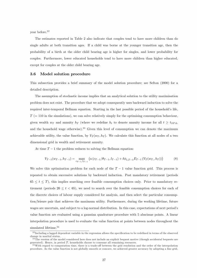
3.6 Model solution procedure

This subsection provides a brief summary of the model solution procedure; see Sefton (2000) for a

detailed description.

The assumption of stochastic income implies that an analytical solution to the utility maximisation

problem does not exist. The procedure that we adopt consequently uses backward induction to solve the

required inter-temporal Bellman equation. Starting in the last possible period of the household’s life,

T (= 110 in the simulations), we can solve relatively simply for the optimising consumption behaviour,

given wealth wT and annuity hT (where we redefine ht to denote annuity income for all t ≥ tSPA,

and the household wage otherwise).33 Given this level of consumption we can denote the maximum

achievable utility, the value function, by VT (wT , hT ). We calculate this function at all nodes of a two

dimensional grid in wealth and retirement annuity.

At time T − 1 the problem reduces to solving the Bellman equation:

VT−1(wT−1, hT−1) = maxcT−1,lT−1

¡u (cT−1/θT−1, lT−1) + δφ1,T−1ET−1 (VT (wT,, hT ))

¢(8)

We solve this optimisation problem for each node of the T − 1 value function grid. This process isrepeated to obtain successive solutions by backward induction. Post mandatory retirement (periods

65 ≤ t ≤ T ), this implies searching over feasible consumption choices only. Prior to mandatory re-

tirement (periods 20 ≤ t < 65), we need to search over the feasible consumption choices for each of

the discrete choices of labour supply considered for analysis, and then select the particular consump-

tion/leisure pair that achieves the maximum utility. Furthermore, during the working lifetime, future

wages are uncertain, and subject to a log-normal distribution. In this case, expectations of next period’s

value function are evaluated using a gaussian quadrature procedure with 5 abscissae points. A linear

interpolation procedure is used to evaluate the value function at points between nodes throughout the

simulated lifetime.34

32 Including a lagged dependent variable in the regression allows the specification to be redefined in terms of the observedchange in marital status.33The version of the model considered here does not include an explicit bequest motive (though accidental bequests are

generated). Hence, in period T , households choose to consume all remaining resources.34With regard to computation time, there is a trade-off between the grid resolution and the order of the interpolation

procedure. As the value function is not globally smooth or concave, we achieved greater accuracy by adopting a fine grid,

27

For the analysis reported in Section 7, we divided the real non-negative domain of both private

income and wealth using a log scale, each comprised of 61 points from ages 20 to 64, and 151 points

during each of the periods from age 65. From age 20 to 89 (inclusive), solutions are required for single

adults and couples. Between ages 25 and 42, solutions are required for 0 to 3 children, and for an

additional 0 to 3 children between ages 34 and 51. Between ages 20 and 64, solutions are required for

a low wage offer on the one hand (in which case households are considered to choose not to supply

labour), and the two labour options on the other. Furthermore, between ages 20 and 64 the dimension

recording a household’s private pension entitlement was divided into 11 points. Hence, the full model

involves calculating solutions to expected lifetime utility maximisation problems at 59,085,995 points

for the simulated lifetime.35

Having solved for the household utility maximising behavioural responses as described above, the

life-courses of individual households are simulated by running households forward through the grids.

For example, given a household’s initial wealth, wage offer, and number of adults (w20,ϕ20, h20, na20)

we read off from the age 20 grid the household’s optimal choice of consumption and leisure (c20, l20).

Then three random draws are taken: one from a uniform distribution that is compared against the

probability implied by equation (7) to determine the number of adults at age 21, na21; another from

a uniform distribution to determine whether a high wage offer is made ϕ21; and the third from the

distribution ωi,t ∼ N¡0,σ2ω

¢, to obtain the household wage rate at age 21 described by equation (6),

h21. Equation (3) is also used to calculate the household’s wealth, so that all four state variables for age

21 are determined, (w21,ϕ21, h21, na21). This process is repeated for t = 21, 22, ...T . A cohort is built up

by repeating this procedure for a sample of households. Our analysis is based on the data generated

for this synthetic population. We now discuss some technical issues that arise in the optimisation

procedure.

The value function in this problem is neither smooth, nor concave (though it is increasing and

continuous). This is because the labour supply decision is discrete and the budget set is non-convex (due

to means testing of welfare benefits). Non-concavities of the value function imply that the optimisation

problem (8) can have local maxima, a problem that can be addressed in a number of alternative ways.

French (2005), for example, adopts a brute-force method by searching across the grid that defines all

possible choice combinations of the assumed control variables. This is very time consuming, which

and a linear interpolation routine. Both the wealth and wage grid dimensions were specified on a log scale (to providegreater detail at the low end of the distribution).35=151*151*((110-89)+2*(89-64))+61*61*2*3*11*((64-51)+4*(51-42)+4*4*(42-33)+4*(33-24)+(24-19)) Tests were

conducted with a finer grid structure, based upon 101 points for each of the wealth and private income dimensions,to which the simulated behaviour was insensitive. This full model required just over 17 hours to run on an Intel X6800processor. Most of the runs undertaken to calibrate the model were undertaken without concavity checks, by adopting acourse grid structure, and by omitting pension wealth (but assuming forced annuitisation at age 65). These simplificationsreduced the model run time to just under 15 minutes on a Pentium D processor.

28

complicates calibration and associated analysis. We therefore chose to solve the Euler equations (for

consumption), and guard against the selection of a local optimum. This was relatively straightforward

for our decision problem, as we were searching over only one continuous variable (consumption). The

procedure that we adopt is described as follows.

For a given discrete labour supply choice, we searched for a solution to the Euler equation over all

feasible (bounded) consumption choices using the Bus & Dekker (1975) bisection algorithm. Having

found one solution, we searched above and below for an alternative solution.36 If we found one, we

searched recursively for any further solutions above and below. This was repeated until all solutions

were found. From these solutions we selected only those that were feasible.37 Of all feasible solutions,

the one that maximised the value function was selected. This procedure was repeated for all possible

discrete labour choices, and the maximum over the labour choices was selected.

3.7 Summary

• The rational agent model considers household decisions regarding consumption and labour supplyat annual intervals throughout a life course that extends from age 20 to the maximum potential

age of 110.

• Household heterogeneity is described by eight characteristics: age, education, number of adults,number of children, potential wage, net liquid wealth, pension rights, time of death; where the

characteristics in italics are generated stochastically.

• Intertemporal preferences are time separable, and take a Constant Relative Risk Aversion (CRRA)form.

• Intratemporal preferences between consumption and leisure take a Constant Elasticity of Substi-tution (CES) form.

• Expected lifetime utility is considered to be maximised, subject to an age specific liquidity con-straint that permits the holding of unsecured debt.

• The interest charged on unsecured debt is an increasing function of a household’s debt to incomeratio.

• Taxes and benefits are specified to reflect the UK transfer system as it stood in 2003.36This involved projecting a limited grid about an identified local maximum, and evaluating the first order condition

for the Euler maximisation problem at each point on the limited grid. If the first order condition at a point on thelimited grid below (above) the initial local maximum was found to have the opposite sign to it’s value just slightly below(above) the originally identified local maximum, then the bisection algorithm was reapplied to solve the associated Eulerconditions for a new local maximum.37This was a check that marginal change in the value function with respect to wealth was locally increasing. Non-

smoothness in the value function implies jumps in marginal rates. The interpolation routines will tend to smooth thesejumps, possibly introducing an infeasible solution to the Euler equation.

29

• Income dynamics are modelled by a regression toward the mean process.

• The model is solved numerically by backward induction.

We now describe the methods used to calibrate the parameters of the model.

4 Model Calibration

The parameters of the model were adjusted to match the characteristics by age of a simulated population

to those described by household micro data. Calibration was undertaken using the following gird-search

procedure. First, wealth at age 20 was set to 0. lW,na was set to 0.5 for both couples and singles (working

entails a 50% reduction in leisure). We then normalised by the price of consumption so that wages and

interest rates were specified in real terms. The real interest rate was fixed at 4 percent per annum for

non-negative wealth balances¡rI¢, the lower limit cost of debt

¡rDl¢was set to 7 percent, and the upper

limit¡rDu¢to 15 percent. This range of interest charges for household debt is based upon averages

between January 2000 and August 2005 (the most recently available data at the time of writing) of

the end of month average interest rates charged on unsecured personal loans for the lower bound, and

of the end of month weighted average interest rates charged on credit cards for the upper bound, as

reported by the Bank of England.38

The credit limit, Dt, that is considered for analysis is specified to provide maximum flexibility, while

at the same time ensuring that households have no debt from age 65, and omitting the possibility of

numerical errors in the solution procedure. A numerical error will result if a household is required

to consume less than or equal to zero in any period to satisfy the imposed budget constraint. This,

combined with the assumption that all households must have paid off their debts by age 65, resulted in

the adoption of an age specific credit limit that is defined in terms of the minimum disposable income

stream that is permissable under the analysis.

In defining the assumed credit limit, we took the lowest potential disposable annual income at any

age (as described by the considered tax and benefits system), deducted a £5 disregard, and calculated

the cumulative discounted value to age 65 implied by the maximum assumed interest charge on debt.

The resultant age specific credit limits are reported in Table 4, and indicate that the assumed credit

limit is over £20,000 for most of the working lifetime. To help identify how the assumed credit limit

relates to the actual circumstances of households in the UK, Table 3 reports distributional statistics for

unsecured debt identified by four recent surveys.39 Table 3 indicates that most households that take38The average between January 2000 and June 2007 of the end of month interest rate charged on unsecured personal

loans reported by the Bank of England (code IUMHPTL), is 9.3 percent, and for credit card debt (code IUMCCTL) is16.5 percent. Discounting by the Consumer Prices Index (ONS code D7G7) for the same period, gives real interest ratesof 7.6 and 14.7 percent respectively.39The surveys include a study commissioned by the Bank of England (Tudela & Young (2003)), a study commissioned

by the CAB (2003), a study by KPMG (2003), and a study by Kempson (2002).

30

Table 3: Distribution of the Amount Owed by Debtors (Unsecured Debt)

S ou r c e : Ta b le D , Tu d e la & You n g ( 2 0 0 3 )

out unsecured loans in the UK borrow small amounts. Importantly, no more than 2% of households

interviewed on behalf of the Bank of England or the Citizens’ Advice Bureaux, and 7% of households

interviewed for KPMG, held unsecured debts totalling £20,000 or more.40

Having defined the model parameters referred to above, we then selected a starting value for each of

the remaining parameters, against which a solution to the lifetime optimisation problem was obtained

following the methods described in Section 3.6. Monte-Carlo methods were used to generate the life-

history for a cohort of households, based upon the behavioural responses described by the model solution,

and the stochastic processes assumed for the intertemporal development of agent specific state variables.

Calibration proceeded by comparing the characteristics by age of the simulated cohort with age profiles

that were estimated from survey data.

The model was calibrated three times: first against age profiles estimated from survey data for a

representative sample of the entire UK population, and then against age profiles estimated for lower ed-

ucated households, and finally for higher educated households. The first calibration involved matching

the model to distributional statistics for labour supply, disposable non-property income, and consump-

tion. For the education specific subgroups, only the income parameters of the model were altered, so

that all of the simulations reported in Sections 7 and 8 are based upon the same (unobservable) prefer-

ence parameters. Furthermore, due to the absence of required survey data, none of the calibrations are

matched directly to measures of household wealth or debt. This is of note, given our focus on household

indebtedness.

Outline

The section begins by describing the sample statistics against which the model was calibrated. It

then discusses issues related to calibration of the income processes and preference parameters, before

reporting the calibrated parameters. The age profiles against which the model was calibrated are

40More recently, 5% of debtors reported debts in excess of £20,000 to a survey undertaken in September 2006 by NMGResearch for the Bank of England. See Waldron & Young (2006), p. 398.

31

reported alongside the calibrated parameters for the calibration to the representative sample of the full

UK population, and for the education subgroups in Appendix C.

4.1 The data

To calibrate our model we require age profiles at the household level for both singles and couples of41:

1. The proportion of households with at least one member employed, by education status

2. The mean of household private non-property income (gross of taxes and benefits), by education

status

3. The variance of household private non-property income, by education status

4. The mean of household disposable income (net of taxes and benefits)

5. The variance of household disposable income

6. The mean of household total consumption

7. The variance of household total consumption

The parameters of models similar to the type considered here are usually matched against moments

estimated from one of three survey data sources. The first is (pseudo) panel data for an actual cohort.

These data are affected by time and cohort effects that make them unrepresentative for the population in

general.42 Alternatively, it is possible to control for time and cohort effects by econometric estimation.

In this case, collinearity between age, cohort and time implies the need to introduce an additional

restriction to permit identification. One popular restriction, suggested by Deaton (1997), is to assume

that time effects average out over the long run. This assumption produces estimated age profiles that

represent an average taken over all cohorts included in the (pseudo) panel data set used for estimation.

Calibrating the model against this sort of age profile implicitly assumes that behaviour is invariant

to changes in the policy environment during the period of estimation, which is an assumption that is

difficult to maintain when one of the objectives of the analysis is to consider behavioural responses

to alternative policy experiments.43 The third approach involves matching the model against suitably

adjusted age profiles described by cross-sectional survey data.

We adopted the third approach referred to above for the study reported here. The cross-sectional

data considered for the calibrations describe the decisions of agents given their prevailing circumstances.41 Statistics of household wealth are prominently omitted from this list due to the limited nature of wealth data that

are currently available for the UK. Nevertheless, a “sanity check” was performed by comparing age averages for wealthgenerated by the model against sample statistics imputed from the 2000/01 wave of the BHPS. These are available fromthe author upon request.42 See, for example, Attanasio et al. (2005).43 See, for example, Sefton et al. (2007).

32

Unfortunately, however, they do not provide details regarding agents expectations regarding the future.

This problem is exacerbated in the current context, where assumptions regarding wage growth are likely

to influence preferences toward indebtedness. And if one admits the importance of wage growth in the

analysis, then other aspects of the cross-sectional policy environment begin to demand adjustment, such

as the specification of tax rates and thresholds.

We have opted to calibrate the model against age profiles calculated from the cross-sectional micro

data provided by the 2001/02, 2002/03, and 2003/04 waves of the Expenditure and Food Survey,

adjusting all financial characteristics for wage growth of 1.9% per annum.44 This figure for wage

growth is on the high end of the historical variation, and reflects our current interest in considering

whether, given plausible assumptions for individual expectations, contemporary consumer borrowing

can be explained by the rational agent model described here.

Taxes and benefits in the model are also based upon an adjusted form of the UK transfer system as

it was applied in 2003.45 Regarding the adjustments made to the transfer system, comparisons between

the simulated profiles and survey data for private and disposable income would be simplified if the wage

growth indexing applied to the financial characteristics described by survey data was also applied to

the various thresholds that are assumed for the tax system. This was not done, however, as such an

assumption would provide a widely inaccurate reflection of the practical reality: threshold rates tend to

grow at the rate of price inflation, and benefits by more than the rate of price inflation, but by less than

wage growth. We have consequently held tax rates and thresholds fixed (in real terms), and projected

welfare benefits to grow by 1 percent per year (less than the 1.9 percent assumed for wage growth).

The criteria that are assumed here for calibrating the model depend upon clear value judgements

about agent expectations. Ideally, we would test how sensitive the analytical conclusions of this study

are to the basis considered for calibration. That issue remains a subject for further research.

4.2 Calibration of the income process

The wage generating process was calibrated by comparing simulated and sample statistics for the

distribution of household private non-property income by age. Comparisons based upon the distribution

of household disposable non-property income then provide an indication of how closely the simulated

tax and benefits policy reflects the practical reality, as described by survey data.

Four aspects of the wage generating process were subject to detailed calibration for each of singles

44Based on real household disposable (equivalised) income growth for the period 1971-2002, as reported in Figure 5.14of Social Trends 34 (ONS publication). Growth calculated with respect to household age — i.e. yt,i = zt,i.1.019(t−k(i)),where z denotes the respective financial characteristic (consumption, private income, or disposable income) as describedby survey data, y denotes the value considered for calibration, i refers to the sample wave, k (i) takes the value 20 for the2003/04 EFS wave, 19 for the 2002/03 wave, and 18 for the 2001/02 wave, and t denotes household age.45This approach may be contrasted with that of Nelissen (1998) who explores redistribution using a microsimulation

model that is designed to capture the historical variation observed in Dutch tax and benefits policy.

33

and couples (and for each education subgroup). First, the parameters defining the initial distribution

of wages¡µna,20,σ

2na,20

¢were selected to reflect statistics of the distribution for private non-property

income at age 20. Second, the intertemporal persistence term³βnai,t

´was increased to motivate higher

labour supply by the young, and to smooth the rate of labour market departure at older ages. Third, age

specific dummy variables (one for each year) and the variance of the household specific disturbance term³σ2ω,nai,t

´were adjusted to match the age profile of the distribution of private non-property income

to the profiles estimated from survey data. And finally, the (age independent) probability of a low

wage offer (ϕ) was adjusted to match the level of the proportion of the respective population (singles

or couples) employed — this parameter was introduced into the model as we were otherwise unable to

capture the discretely lower rates of employment observed for single households (a limitation that is

explained, in part, by the fact that we do not include an explicit allowance for child-care in our model).

4.3 Calibration of preference parameters

There are four preference parameters to calibrate, γ, ε, δ, and α. The parameter pair (γ, δ) tend to

determine household preferences over feasible intertemporal expenditure paths, and the parameter pair

(ε,α) affect preferences over feasible intratemporal consumption/leisure choices.46 These parameters

were adjusted to match the model against age profiles estimated for the full UK population.

For given values of the elasticity parameters γ and ε, we chose the discount rate, δ, to achieve

the ‘closest’ match between the simulated and estimated age profiles for mean household consumption;

and we chose the parameter α to match average retirement rates. Effectively this process defines the

parameters (δ,α) as a function of (γ, ε). Additional criteria were therefore required to select the

parameters (γ, ε).

It can be shown (see Sefton et al. (2006)) that increasing ε, decreases the demand for leisure relative

to consumption for high income households (equivalent to later retirement in the model), but has the

opposite influence on low income households. Hence, ε was adjusted to match the cross-sectional timing

of retirement. Increasing γ tends to exaggerate the influence of disparities between the interest rate (r)

and the discount rate (δ) on the time profile of consumption. Furthermore, as noted by Heckman (1974),

consumption will tend to track labour income under the life-cycle hypothesis if leisure and consumption

are direct substitutes in utility. A smaller value of γ, ceteris paribus, implies greater substitutability

between leisure and consumption, and hence more pronounced income tracking. We therefore adjusted

γ to fit the distribution of consumption about the mandatory retirement age, when labour changes most

substantially. See Sefton et al. (2006) for detailed statistics indicating the sensitivity of the simulations

46This division does not strictly hold because the experience effect on wages invalidates two-stage budgeting. Never-theless, it does provide a reasonable approximation, particularly toward the age of retirement, when the experience effecton wages has a dampened influence on individual behaviour.

34

to alternative assumptions regarding γ and ε.

4.4 The fit between simulated and sample age profiles

We begin by discussing statistics associated with calibration of the model to sample statistics estimated

for the full UK population, before moving on to discuss calibrations for the education specific subgroups.

The representative sample

Following an extensive search, our preferred parameter values are reported in Table 4. The table is

divided into three panels. The top panel reports preference parameters and other exogenously assumed

population characteristics, the middle panel reports parameters for the wage generating process, and

the bottom panel provides age specific dummy variables.

The calibrated parameter combination implies that consumption and leisure are direct substitutes,

and is associated with an average intertemporal elasticity of substitution for consumption of 0.52, which

lies within the range of values considered by the literature.47 The parameters assumed for the wage

generating process imply strong intertemporal persistence. The survival probabilities assumed for the

analysis are based upon the probability that at least one member of a couple survives from age 20,

and were calculated from statistics reported in the life tables published by the Government Actuary’s

Department for the UK for years 2001-2003, (the most recent period which GAD projections were

available).48

The relation between the simulated statistics obtained from the model using the calibrated parameter

values reported in Table 4, and the statistics calculated from survey data are displayed in Figures 8 to

11. The statistics calculated from the simulated data are referred to as “simulated statistics”, and those

calculated from survey data are referred to as “sample statistics”. All monetary values are reported

relative to average gross annual income for all full-time employees in the UK during 2003/04, equal to

£22,72449.

Figures 8 to 11 indicate that, in spite of the strong assumptions upon which the model is based, a

close match was obtained between the simulated and sample statistics. Starting with Figure 8, the top

panel indicates that a reasonably close match was obtained to the age profile of employment for both

47Calculated at population averages at age 45 for consumption (£557 per week), leisure (0.9), and the equivalence scale(1.804 * 470). Simulations undertaken by Auerbach & Kotlikoff (1987) are based upon an intertemporal elasticity ofsubstitution of 0.25 (coefficient of risk aversion of 4), while Cooley & Prescott (1995) consider a value of 1. Grossman &Shiller (1981), Mankiw (1985) and Hall (1988) report econometric estimates for the intertemporal elasticity between 0 and0.4, Blundell et al. (1994) report an estimate of 0.75, while Hansen & Singleton (1983), Mankiw et al. (1985), and Ziliak& Kniesner (2005) report estimates of approximately 1. Values of the coefficient of risk aversion required to explain theequity premium puzzle (Mehra & Prescott (1985)) imply very small elasticities of intertemporal substitution, althoughevidence from attitudinal surveys suggest that the value is unlikely to be less than 0.2 (Barsky et al. (1997)).48On 31 January 2006, responsibility for the production of national life tables transferred to the Office

for National Statistics (ONS). Current and historic life tables are still available on the GAD website at:http://www.gad.gov.uk/Life_Tables/Life_tables_background.htm.49Average gross annual income for all full-time employees reported for winter 2003/04 (Labour Force Survey Historical

Quarterly Supplement, Table 37, available from the National Statistics website: http://www.statistics.gov.uk/).

35

Table 4: Calibrated Model Parameters for Representative Sample of UK PopulationGeneral Model Parameters

intertemporal elasticity (gamma) 0.51 interest rate on investments (%) 4.00 intratemporal elasticity (epsilon) 0.55 interest rate on debt, lower bound (%) 7.00 utility price of leisure (alpha) 0.66 interest rate on debt, upper bound (%) 15.00 discount rate (delta) 0.98 wealth at age 20 0.00

Wage Generating Parameterssingles couples

mean log wage at age 20 5.00 5.50standard dev of log wage at age 20 0.10 0.10wage persistence (beta) 0.90 0.90standard dev of log wage from age 21 0.35 0.30probability of low wage offer (phi) 0.30 0.05

Age Specific Dummy Variablesage m(t) singles m(t) couples credit limit grid points age survival rate* grid points20 1.000 6.942 19952.74 245586 65 0.997 4560221 1.888 12.428 20158.45 245586 66 0.996 4560222 3.872 18.968 20366.63 245586 67 0.996 4560223 7.130 27.936 20577.35 245586 68 0.995 4560224 11.554 39.991 20790.73 245586 69 0.994 4560225 17.818 53.951 21006.85 982344 70 0.993 4560226 25.833 71.015 21225.85 982344 71 0.991 4560227 35.845 91.250 21447.86 982344 72 0.989 4560228 47.371 114.223 21673.03 982344 73 0.987 4560229 60.453 140.342 21901.54 982344 74 0.984 4560230 74.685 169.305 22133.58 982344 75 0.981 4560231 91.613 201.059 22369.38 982344 76 0.978 4560232 109.382 236.094 22609.18 982344 77 0.974 4560233 128.904 273.995 22853.27 982344 78 0.970 4560234 148.544 314.290 23101.99 3929376 79 0.965 4560235 169.814 356.355 23355.70 3929376 80 0.959 4560236 190.578 399.815 23614.83 3929376 81 0.953 4560237 211.919 442.538 23879.87 3929376 82 0.946 4560238 232.691 487.035 24151.37 3929376 83 0.937 4560239 255.758 531.893 24429.97 3929376 84 0.928 4560240 279.013 577.142 24716.41 3929376 85 0.914 4560241 302.059 622.234 25011.51 3929376 86 0.903 4560242 325.779 664.874 25316.22 3929376 87 0.890 4560243 352.518 704.218 25631.66 982344 88 0.876 4560244 377.770 745.003 25959.07 982344 89 0.859 4560245 400.999 782.421 26299.90 982344 90 0.846 2280146 423.420 817.691 26655.81 982344 91 0.830 2280147 442.641 850.879 27028.69 982344 92 0.810 2280148 461.247 882.637 27420.72 982344 93 0.787 2280149 477.074 909.949 27834.42 982344 94 0.772 2280150 490.054 933.874 28272.66 982344 95 0.749 2280151 498.650 949.910 28738.75 982344 96 0.731 2280152 499.827 955.071 29236.48 245586 97 0.710 2280153 492.924 949.269 29770.22 245586 98 0.692 2280154 480.399 936.375 30344.99 245586 99 0.676 2280155 458.006 910.519 30966.54 245586 100 0.650 2280156 428.937 876.902 30437.11 245586 101 0.611 2280157 385.408 822.972 29775.99 245586 102 0.578 2280158 340.386 759.827 28962.93 245586 103 0.526 2280159 296.949 697.309 27974.59 245586 104 0.475 2280160 256.692 636.859 26784.15 245586 105 0.416 2280161 219.200 578.145 22949.09 245586 106 0.349 2280162 198.645 541.325 18459.73 245586 107 0.270 2280163 176.663 502.568 13217.13 245586 108 0.187 2280164 165.885 480.725 7107.51 245586 109 0.100 22801

110 0.000 22801m(t) = age specific dummy veriables in wage generating processcredit limit = maximum debt households can draw upongrid points = no of points by age at which a solution is obtained to the utility maximisation problem (no allowance for personal pensions)* survival rate = probability of surviving to age t+1 given survival to age t

36

0

0.1

0.2

0.3

0.4

0.5

0.6

0.7

0.8

0.9

1

20 25 30 35 40 45 50 55 60 65

age

prop

ortio

n of

pop

ulat

ion

Sample statistics - couples Sample statistics - singles Simulated statistics

couples

singles

Panel A: Proportion employed by age and relationship status

0

10

20

30

40

50

60

1 2 3 4 5

wealth quintile

prop

ortio

n no

t em

ploy

ed

simulated statistics ELSA

Panel B: Distribution of early retirement — ages 55 to 59N o te s : S am p le s t a t i s t ic s — a g e p r o fi l e s c a lc u la t e d f r om E x p e n d it u r e a n d Fo o d S u rv e y d a t a , 2 0 0 1 / 0 2 , 2 0 0 2 / 0 3 , a n d 2 0 0 3 / 0 4

S im u la t e d s t a t i s t i c s — a g e p r ofi l e s g e n e r a t e d f r om m o d e l , u s in g c a l ib r a t e d p a r am e t e r s r e p o r t e d in Ta b le 4

E L SA — p e r c e n t a g e o f m e n a g e d 5 5 -5 9 e c o n om ic a l ly in a c t iv e by w ea lt h q u in t i l e , 2 0 0 2 / 0 3 w av e o f t h e E n g l i s h

L o n g i t u d in a l S tu d y o f A g in g , Ta b le 4A .1 2 , M a rm o t e t a l . ( 2 0 0 3 )

Figure 8: Timing of Retirement — simulated versus survey data

37

0

0.5

1

1.5

2

2.5

3

20 25 30 35 40 45 50 55 60 65age

prop

full-

time

emp

inco

me

Sample statistics - couples Sample statistics - singles Simulated statistics

Geometric Mean of Private Non-Property Income

singles

couples

00.20.40.60.8

11.2

20 25 30 35 40 45 50 55 60 65age

varia

nce

Variance of log Private Non-Property Incomesingles

00.10.20.30.40.50.60.7

20 25 30 35 40 45 50 55 60 65age

varia

nce

Simulated statistics Sample statistics

couples

N o t e s : S am p le s t a t i s t i c s — a g e p r ofi l e s c a l c u la t e d f r om E x p e n d i t u r e a n d Fo o d S u rve y d a t a , 2 0 0 3 / 0 4

S im u la t e d s t a t i s t ic s — a g e p r o fi l e s g e n e r a t e d f r om m o d e l , u s in g c a l ib r a t e d p a r am e t e r s r e p o r t e d in Tab le 4

M on e t a ry va lu e s r e p o r t e d a s p r o p o r t io n s o f ave r a g e a n nu a l fu l l - t im e em p loym en t in c om e fo r 2 0 0 3 / 0 4 , e q u a l t o £ 2 2 ,7 2 4

Figure 9: Private Non-Property Income Profiles by Age — simulated versus survey data

38

0

0.5

1

1.5

2

2.5

20 25 30 35 40 45 50 55 60 65age

prop

of f

ull-t

ime

empl

oym

ent i

ncom

e

Sample statistics - couples Sample statistics - singles Simulated statistics

Geometric Mean of Disposable Non-Property Income

singles

couples

0

0.2

0.4

0.6

0.8

1

20 25 30 35 40 45 50 55 60 65age

varia

nce

Variance of log Disposable Non-Property Income

singles

0

0.2

0.4

0.6

0.8

1

20 25 30 35 40 45 50 55 60 65age

varia

nce

Simulated statistics Sample statistics

couples

N o t e s : S am p le s t a t i s t i c s — a g e p r ofi l e s c a l c u la t e d f r om E x p e n d i t u r e a n d Fo o d S u rve y d a t a , 2 0 0 3 / 0 4

S im u la t e d s t a t i s t ic s — a g e p r o fi l e s g e n e r a t e d f r om m o d e l , u s in g c a l ib r a t e d p a r am e t e r s r e p o r t e d in Tab le 4

M on e t a ry va lu e s r e p o r t e d a s p r o p o r t io n s o f ave r a g e a n nu a l fu l l - t im e em p loym en t in c om e fo r 2 0 0 3 / 0 4 , e q u a l t o £ 2 2 ,7 2 4

Figure 10: Disposable Non-Property Income Profiles by Age — simulated versus survey data

39

0

0.2

0.4

0.6

0.8

1

1.2

1.4

1.6

1.8

20 30 40 50 60 70 80age

prop

of f

ull-t

ime

empl

oym

ent i

ncom

e

Sample statistics - couples Sample statistics - singles Simulated Statistics

Geometric Mean of Household Consumption

singles

couples

children of f irst birth year leave household

children of second birth year leave household

State Pensionable Age

00.10.20.30.40.50.60.7

20 30 40 50 60 70 80age

varia

nce

Variance of log Consumption

singles

0

0.1

0.2

0.3

0.4

0.5

20 30 40 50 60 70 80age

varia

nce

Sample statistics Adjusted statistics

couples

N o t e s : S am p le s t a t i s t i c s — a g e p r ofi l e s c a l c u la t e d f r om E x p e n d i t u r e a n d Fo o d S u rve y d a t a , 2 0 0 3 / 0 4

S im u la t e d s t a t i s t ic s — a g e p r o fi l e s g e n e r a t e d f r om m o d e l , u s in g c a l ib r a t e d p a r am e t e r s r e p o r t e d in Tab le 4

M on e t a ry va lu e s r e p o r t e d a s p r o p o r t io n s o f ave r a g e a n nu a l fu l l - t im e em p loym en t in c om e in 2 0 0 3 / 0 4 , e q u a l t o £ 2 2 ,7 2 4

Figure 11: Consumption Profiles by Age — simulated versus survey data

40

singles and couples. The most pronounced departure between the simulated and sample statistics for

the proportions of the population employed occurs between ages 20 and 25, with the simulation model

generating excessive proportions of the population employed for both singles and couples. This is

attributable to our omission from the model of education, and the focus of the model on labour supply,

subject to an age independent probability of a low wage offer. The excess employment generated

during early ages is likely to reduce the extent of indebtedness generated by the rational agent model,

and should be borne in mind when interpreting the analysis presented in Section 7. In contrast, the

simulation model appears to do a very good job of capturing the relation between age and retirement

described by the sample statistics.

The bottom panel of Figure 8 indicates that the simulation model approximates the distribution of

early retirement described by sample statistics, with earlier retirement at the distributional extremes,

and later retirement in the middle quintiles. It is of note, however, that the model generates earlier

retirement amongst households in the highest wealth quintile than it does for households in the poorest

quintile, in contrast with the associated sample statistics. As noted in Section 4.3, this match is

controlled by adjusting the intra-temporal elasticity of substitution between consumption and leisure —

increasing ε tends to bring forward the retirement age of poorer households and delay the retirement of

richer households. Our calibration sets ε = 0.55, a value that is at the upper end of the range identified

in the related empirical literature (see, for example, Stern (1976)), and was selected after extensive

experimentation.

With regard to the alternatives that were considered, we found that the match between the simulated

and sample statistics reported in the bottom panel of Figure 8 could be improved by increasing ε.

However, it was found that an ‘unreasonably’ high ε = 0.9 was required to approximate the distribution

of early retirement as described by the sample statistics reported in the bottom panel of Figure 8.

Furthermore, increasing ε had an important influence on other aspects of the model calibration — most

notably the substitutability between consumption and leisure. Increasing ε, ceteris paribus, increases

the substitutability between consumption and leisure. This distorts the consumption profile, an effect

that can be offset by a coincident increase in γ. γ in turn influences the intertemporal elasticity of

consumption, and the responsiveness of households to interest rates, which necessitates an adjustment

of the discount factor δ to control for associated distortions to the consumption profile. Unfortunately,

each of the adjustments referred to above are imperfect controls, in the sense that they also result in

secondary effects. As a consequence, we found that increasing ε — while it could improve the distribution

of early retirement as described in Figure 8 — obtained a poorer fit of the model in general.

The top panel of Figure 9 reports statistics for private (pre tax and benefit) non-property income.

The two panels of the figure indicate that a close match was obtained to the age profiles of both the

41

geometric mean and variance of private non-property income, for both singles and couples. In contrast,

the simulated statistics for disposable (post tax and benefit) non-property income reported in Figure

10 suggest that the model understates the geometric mean described by survey data for both singles

and couples, and overstates the associated variances. These disparities between the match obtained

to private non-property income and disposable non-property income are to be anticipated, given the

different adjustments applied to the financial characteristics described by survey data on the one hand,

and to taxes and benefits on the other. Furthermore, they reflect the imperfect fit obtained between

the simulated and sample statistics for household labour supply, the stylised specification assumed

for taxation in the model, and the fact that the model makes no allowance for mis-representation,

miscalculation, or reporting errors that are likely to affect survey data.

The top panel of Figure 11 indicates that the model captures the more pronounced hump shape

by age observed for two adult households than for singles, which is in part attributable to the higher

propensity of couples to have dependent children.50 It was surprising to note that there is no appreciable

fall in consumption about age 65 described by the sample statistics, an effect that is found in cross-

sectional surveys for earlier time periods and has motivated substantial interest in the literature. In the

current context, this observation made it necessary to set ε and γ to similar values, toning down the

substitutability that is necessary to match similar models to earlier empirical data (see, for example,

Sefton et al. (2007)). The profiles for the geometric mean of consumption suggest that the model

generates a little too much saving by singles, and too little saving by couples. It is difficult to address

these disparities in the current context, where the only differences between the two types of household

are considered to be in terms of the wage generating process, tax treatment, and consumption needs.

With regard to the statistics reported in the bottom panel of Figure 11, the model understates the

variance of consumption by age for both couples and singles described by the survey data. This may

indicate too much intertemporal smoothing in the simulation model, or too much income mobility.

With regard to the second of these two possibilities, it is of note that we assume a high value for the

intertemporal persistence of the wage generating processes, β, for both singles and couples.

As noted above, although the wealth data available for UK households were considered to be inad-

equate for the purpose of calibrating the model, imputed wealth data taken from the 2000/01 wave of

the BHPS were considered following the model calibration to check whether the implications for saving

could be considered sensible. The relevant statistics are reported in Figure 12. These suggest that the

simulation model does a reasonably good job of capturing both the rate of accrual and dispersal of

50The sample statistics for geometric means of consumption by age for both singles and couples were proportionallyadjusted to match the implied lifetime averages (weighting each age equally) to the associated simulated statistics. Thisadjustment, equal to a 21 percent increase for singles and a 3 percent decrease for couples, was applied to ensure that thecalibration with respect to consumption was not affected by disparities associated with disposable income or the lifetimebudget constraint that is applied in the model.

42

-2

0

2

4

6

8

10

12

14

16

20 30 40 50 60 70 80 90

age

prop

ortio

n of

full-

time

emp

inco

me

sample statistics simulated statistics

Figure 12: Wealth Profiles by Age — simulated versus survey data

wealth described by the associated survey data.

Calibrations distinguished by level of education

The parameters of the model that describe the wage generating process were adjusted to reflect sample

statistics for private non-property household income of population subgroups distinguished by level

of education. The education specific sample statistics were based upon the same EFS data as were

considered for the full population, but divided into two subgroups distinguishing households by whether

at least one member had full-time education beyond the age of 16. This divided the sample population

into two roughly equal halves (44% of households being identified in the higher educated subgroup).

The education specific model parameters are reported in Table 5 and the relation between simulated

and survey data are presented in Appendix C.

4.5 Summary

• We have calibrated the model described in Section 3 to survey data derived from the 2001/02,

2002/03, and 2003/04 waves of the Expenditure and Food Survey, adjusting the cross-sectional

survey data to reflect wage growth of 1.9% per annum.

• The model was calibrated against age profiles that are representative of the full UK population,

and for population subgroups distinguished by level of education.

• The model does a good job of capturing the moments against which it has been calibrated, despitethe strong assumptions upon which it is based.

43

Table 5: Calibrated Model Parameters for Population Sub-samples Distinguished by Level of EducationGeneral Parameters

full population lower educated higher educatedsingles couples singles couples singles couples

mean log wage at age 20 5.00 5.50 4.80 5.65 5.00 5.50sd log wage at age 20 0.10 0.10 0.10 0.10 0.10 0.10wage persistence (beta) 0.90 0.90 0.90 0.90 0.90 0.90sd log wage from age 21 0.35 0.30 0.35 0.27 0.35 0.27probability of low wage offer (phi) 0.30 0.05 0.39 0.09 0.20 0.05

Age Specific Dummy Variablesfull population lower educated higher educated

age m(t) singles m(t) couples m(t) singles m(t) couples m(t) singles m(t) couples20 1.000 6.942 1.000 6.942 1.000 6.942 21 1.888 12.428 1.915 11.648 2.160 12.180 22 3.872 18.968 3.333 16.623 4.803 18.853 23 7.130 27.936 5.667 23.386 9.025 28.039 24 11.554 39.991 8.962 32.155 14.828 40.313 25 17.818 53.951 13.563 41.949 22.946 54.928 26 25.833 71.015 19.517 53.950 33.335 73.220 27 35.845 91.250 27.225 68.290 46.165 95.292 28 47.371 114.223 36.054 84.736 61.040 120.643 29 60.453 140.342 46.541 103.488 77.996 150.246 30 74.685 169.305 58.028 124.662 96.963 183.926 31 91.613 201.059 72.310 148.231 118.044 221.744 32 109.382 236.094 86.724 174.134 140.568 264.315 33 128.904 273.995 102.221 203.103 163.853 310.583 34 148.544 314.290 118.199 234.732 186.978 359.801 35 169.814 356.355 136.924 268.693 211.251 410.286 36 190.578 399.815 154.524 304.855 235.765 461.407 37 211.919 442.538 173.682 341.884 261.163 510.913 38 232.691 487.035 191.710 379.097 289.029 563.540 39 255.758 531.893 211.021 416.155 317.602 616.604 40 279.013 577.142 232.272 452.634 346.873 669.227 41 302.059 622.234 253.435 486.920 380.501 722.000 42 325.779 664.874 273.954 518.919 414.330 773.376 43 352.518 704.218 296.138 549.515 447.590 820.307 44 377.770 745.003 317.164 579.258 478.243 868.305 45 400.999 782.421 336.534 607.071 505.309 911.211 46 423.420 817.691 354.307 634.259 527.372 951.720 47 442.641 850.879 372.264 658.904 545.228 992.194 48 461.247 882.637 390.261 684.299 560.700 1031.858 49 477.074 909.949 407.684 705.680 575.516 1069.148 50 490.054 933.874 421.737 722.592 593.797 1107.661 51 498.650 949.910 431.431 735.898 606.456 1136.644 52 499.827 955.071 434.633 747.422 612.712 1155.095 53 492.924 949.269 437.349 750.009 609.939 1162.569 54 480.399 936.375 433.582 751.741 601.068 1157.979 55 458.006 910.519 425.169 748.887 570.513 1135.414 56 428.937 876.902 411.171 727.800 533.139 1100.669 57 385.408 822.972 386.459 702.726 497.002 1039.218 58 340.386 759.827 356.158 667.249 450.114 962.527 59 296.949 697.309 314.400 619.415 389.480 884.859 60 256.692 636.859 277.678 566.689 327.735 806.563 61 219.200 578.145 235.573 524.341 288.767 721.918 62 198.645 541.325 206.234 496.490 257.793 649.256 63 176.663 502.568 172.659 473.853 234.049 588.958 64 165.885 480.725 149.299 451.749 226.356 533.623

m(t) = age specific dummy veriables in wage generating process

44

5 Dis-aggregating Net Wealth to Identify Housing and Collat-eralised Debt

Owner occupied housing is a special type of asset for two reasons. First, it is “lumpy” in a way that few

assets in the typical household balance sheet are. The indivisible nature of housing gives rise to a host

of subsidiary complexities including minimum deposits, mortgage debt, and non-trivial transactions

costs. Secondly, housing is desired for the services that it provides, in addition to the purely financial

considerations that can reasonably be assumed to govern demand for other types of investment. This

means that if housing is included in a model of rational behaviour, then it should enter as a term in

the assumed utility function. These considerations complicate the inclusion of housing in a dynamic

programming model of household savings behaviour, such as the one used for the current study.

Specifically, the current study explores the interactions between saving and unsecured indebtedness

implied by a rational agent model of the household, and how these observations relate to associated

survey data. In this context, housing is important because of its prominence in the aggregate stock

of wealth held by households in the UK, and because of its bearing on secured debt. Unfortunately,

models of the type considered for this study are numerically demanding, and are made more so by the

inclusion of “lumpy” terms in the utility function. To avoid making the model unwieldy, we have had

to make a choice between two options: to include the lumpiness of housing, but omit it from the utility

function, or vice versa.

In our second report submitted under the current project to the DWP in June of 2005, we included

housing in the utility function, but omitted its associated lumpiness. The model used to undertake the

analysis took approximately two days to solve, and the omission of lumpiness from the housing asset was

considered inherently problematic. We have subsequently agreed to include the lumpiness of housing,

but to omit it from the rational decision making environment. In addition to facilitating consideration

of secured debt, this amendment has enabled us to reformulate the model to better capture uncertainty

in household demographics, which has an important bearing on the issue of over-indebtedness and

household savings (as is discussed at length in the sections above).

We use a nested logit model comprised of two levels to project measures of housing wealth and

secured debt on the basis of the other household characteristics that are generated by the dynamic

programming model. The first level of the nested model identifies whether a household is an owner

occupier and, if so, the second level identifies whether they hold mortgage debt. Linear regression models

are then used to identify the value of a household’s housing wealth, and the value of any mortgage that

they may hold.

Although this analytical approach captures aspects of the housing market that were omitted from

45

our second report (such as the lumpiness of housing, and an explicit consideration of mortgage debt),

it is important to note that the approach adopted here to model housing represents an important

methodological departure from the remainder of the study. The basic premise of the analysis is to

consider the relation between debt and savings, as determined by rational economic theory, and how this

bears upon over-indebtedness and welfare in retirement. Modelling housing using reduced form models

is a clear departure from rational economic theory, which should be remembered when interpreting the

results obtained.

The reduced form models used to project measures of housing wealth and collateralised debt were

estimated econometrically using survey data from the BHPS, again adjusted for real wage growth of

1.9% per annum.51 Regression statistics are reported in Tables 6 and 7.

Table 6 indicates that the logit regression considered for analysis does a very good job of capturing

variation observed in the data. The regression statistics indicate that the probability of being a house

owner initially increases with age before levelling out, and finally declining later in life. The probability

of being a house owner also increases, but at a decreasing rate, with labour income and net assets.

Singles, and those with low net liquid wealth are less likely to own their own home, an issue that is

offset somewhat as the value of net debts rise. Finally, house ownership in the previous year is a strong

indicator of house ownership in the current year.

The tobit regression statistics reported in Table 6 indicate that the various characteristics referred to

above have a similar effect on the likely value of housing wealth as they do on the probability of owning

a home. A conspicuous exception is the number of dependent children in a household, which was not

found to have a significant influence on the probability of house ownership, but tends to increase the

value of owner occupied housing. This is consistent with the increase in housing needs that comes with

a larger family.

Table 7 indicates that, amongst house owners, the probability of holding a mortgage is high at young

ages and declines fairly sharply after age 40. Those with higher incomes tend to also have a higher

probability of holding a mortgage, and the probability of holding a mortgage in any year is strongly

correlated with holding a mortgage in the preceding year. Finally, house owners with low net liquid

wealth are also far more likely to hold a mortgage than otherwise similar individuals. Finally, the tobit

statistics reported in Table 7 indicate that the value of a mortgage tends to decrease with the age of a

household, and increase with labour income, house value, and low net liquid wealth.

51The sample was screened to omit those observations with missing data, resulting in a sample size of 6290 used forestimation.

46

Table 6: Regression Statistics for Equations Used to Simulate HousingLogit model for house ownership

full population lower educated higher educatedestimate s.e. estimate s.e. estimate s.e.

const -18.49320 3.631E+00 -24.29840 6.516E+00 -16.98370 5.141E+00age 1.51836 3.384E-01 1.99973 5.860E-01 1.40389 5.024E-01age^2 -0.04164 1.099E-02 -0.05443 1.834E-02 -0.03952 1.727E-02age^3 4.555E-04 1.481E-04 5.919E-04 2.387E-04 4.488E-04* 2.473E-04age^4 -1.780E-06 7.064E-07 -2.287E-06 1.104E-06 -1.855E-06* 1.252E-06lab inc 2.163E-05 6.345E-06 2.151E-05* 1.572E-05 2.176E-05 7.996E-06lab inc^2 -8.587E-11 2.444E-11 -4.451E-11* 1.707E-10 -9.036E-11 2.674E-11dum(single) -0.88502 1.862E-01 -1.06605 3.034E-01 -0.79034 2.456E-01net assets 1.894E-05 2.195E-06 1.836E-05 2.740E-06 2.324E-05 4.615E-06net assets^2 -5.836E-12 6.997E-13 -7.043E-12 1.047E-12 -6.672E-12 2.067E-12net debt 4.439E-05 1.424E-05 6.447E-05 3.209E-05 2.839E-05* 1.561E-05dum(owner t-1) 4.87517 1.990E-01 5.86396 3.359E-01 3.95630 2.481E-01dum(low wealth) -4.01533 2.610E-01 -5.20386 4.591E-01 -2.98517 3.267E-01correct predictions 0.9719 0.9782 0.9604observations 6290 3663 2627prop. with home 0.6458 0.5495 0.7800

Tobit regression for house valuefull population lower educated higher educated

estimate s.e. estimate s.e. estimate s.e.const 45245.50 1.186E+04 60548.30 18152.40 25455.90* 17808.50age -1163.88 4.752E+02 -1278.90 637.61 -302.64* 806.71age^2 3.23396* 4.461E+00 2.26200* 5.56711 -4.35537* 8.19531lab inc 1.33158 7.995E-02 0.21441* 0.19725 1.37654 0.11139lab inc^2 -3.213E-06 4.752E-07 9.492E-06 2.384E-06 -3.522E-06 5.366E-07children 16634.60 3.552E+03 20423.00 5140.40 16750.40 5164.17children^2 -3396.12 1.130E+03 -4528.44 1552.44 -2768.53* 1732.33net assets 8.590E-01 1.157E-02 9.027E-01 0.01659 7.932E-01 0.01758net assets^2 -4.479E-08 7.004E-09 -6.209E-08 1.063E-08 -2.101E-08 9.513E-09net debt 9.226E-01 1.045E-01 4.917E+00 3.731E-01 5.823E-01 1.139E-01lab inc x net assets -3.363E-07 1.225E-07 7.482E-07 3.344E-07 -2.392E-07* 1.460E-07dum(low wealth) -1.337E+05 4.143E+03 -1.526E+05 5.899E+03 -1.126E+05 6.139E+03log likelihood -52620.20 -25890.60 -26568.10Sigma** 86582.6 976.792 77485.7 1247.49 91166.2 1443dum(.) denotes dummy variable* estimate not statistically significant at 95% confidence interval** estimated standard deviation of residualslow wealth defined as net liquid wealth under £5,200 in valuenet liquid wealth = securities + housing - unsec debt - mortgagenet assets / debt taken as + / - measures of net liquid wealth

47

Table 7: Regression Statistics for Equations Used to Simulate MortgagesLogit model for mortgage

full population lower educated higher educatedestimate s.e. estimate s.e. estimate s.e.

const -13.11330 4.100E+00 -15.86430 6.733E+00 -13.76850 5.892E+00age 1.07101 3.605E-01 1.25962 5.684E-01 1.17780 5.430E-01age^2 -0.03277 1.136E-02 -0.03769 1.727E-02 -0.03715 1.794E-02age^3 4.046E-04 1.522E-04 4.579E-04 2.239E-04 4.791E-04* 2.518E-04age^4 -1.801E-06 7.334E-07 -2.001E-06* 1.048E-06 -2.252E-06* 1.270E-06lab inc 2.218E-05 4.244E-06 1.309E-05* 9.415E-06 2.336E-05 5.582E-06lab inc^2 -1.367E-10 3.229E-11 -2.909E-11* 1.133E-10 -1.478E-10 3.792E-11dum(mortgage t-1) 2.95662 1.143E-01 3.28485 1.704E-01 2.66982 1.564E-01dum(low wealth) 4.24672 7.402E-01 4.30573 1.083E+00 4.16113 1.023E+00correct predictions 0.87272 0.88028 0.86920observations 4062 2013 2049prop. with a mortgage 0.52120 0.37904 0.54219

Tobit regression for mortgage valuefull population lower educated higher educated

estimate s.e. estimate s.e. estimate s.e.const -19173.70* 14435.50 2099.76* 24483.20 -86413.10 19662.30age 2969.73 647.64 1068.56* 1023.32 6957.92 942.70age^2 -61.85930 6.71565 -37.95300 9.96360 -111.50200 10.53000lab inc 7.462E-01 4.909E-02 1.115E+00 1.046E-01 5.514E-01 5.651E-02house value 0.07607 0.00722 0.05071 0.01254 0.10001 0.00893dum(low wealth) 3.224E+04 4.959E+03 4.783E+04 8.954E+03 2.503E+04 5.796E+03log likelihood -27423.20 -10057.00 -17326.10Sigma** 69498.6 1126.87 74200.5 2031.92 65374.3 1314.17dum(.) denotes dummy variable* estimate not statistically significant at 95% confidence interval** estimated standard deviation of residualspopulation restricted to home ownerslow wealth defined as net liquid wealth under £5,200 in valuenet liquid wealth = securities + housing - unsec debt - mortgage

S o u r c e : A u th o r c a lc u la t io n s u s in g d a t a f r om w ave s 1 t o 1 0 o f t h e B H P S

5.1 Summary

• Housing is of particular interest in any analysis of private sector indebtedness, due to its indivisiblenature, and the associated implications for mortgage debt.

• The indivisible nature of housing complicates its inclusion in a rational agent model, as does theconsumption by individuals of housing services.

• An adequate treatment of housing within the rational agent framework was consequently consid-ered to lie beyond the scope of the current study.

• The incidence of housing and mortgage debt is modelled in the current project by reduced formregression equations, that were estimated from BHPS survey data.

• The regression coefficients presented here are consistent with a priori expectations.

6 Intuition Behind the Life-cycle Model of Behaviour

This section gives a brief review of the intuition that lies behind the findings that are reported in

Sections 7 and 8. A reader who is familiar with utility theory and the life-cycle model may omit this

48

section without handicap.

The model used to undertake the analysis reported in the current study (described in Sections 3 and

4) implies that, all else being equal, an individual would prefer to smooth their consumption between

two periods, rather than to consume a large amount in one period and very little in another. This is

a property of the function that is assumed to describe individual preferences, and the parameters that

were found to best reflect the survey data against which the model is calibrated. In this context, an

individual will choose to spend more than their income in any given period if they expect that their

consumption “needs” will decline, and/or their income will be higher in future periods.

Consumption needs are considered to be defined by the numbers of adults and children in a house-

hold, by labour supply during the working lifetime, and by the time of death. Three of these four factors

are subject to uncertainty, and the fourth (labour supply) is a choice variable. Expectations regarding

the timing of death influence saving incentives for retirement — the longer an individual believes that

they are going to live, the greater the incentive to save, which competes with immediate consumption

for available credit. In contrast, labour supply tends to increase demand for immediate consumption,

as the preferences considered for analysis imply that consumption and leisure are direct substitutions.

This may arise, for example, due to the costs of working or the desire to unwind after work through

the pursuit of expensive leisure activities. Of course, labour supply also results in higher disposable

income, so that the aggregate effect of working on wealth is usually positive.

The impact of the numbers of adults and children in a household on saving and indebtedness are

more complex. An increase in household size raises consumption needs through the assumption of the

McClement’s equivalence scale, and also raises disposable income through the demographic dependance

assumed for the tax and benefits system. With regard to the number of dependent children, the

adjustments assumed for the tax system more than off-set changes to the assumed equivalence scale,

so that households with dependent children tend to be better off than those without. With regard to

the number of adults, the disposable income of couples is augmented relative to singles by both the tax

system and the wage generating process, which imply that couples tend to be better off than otherwise

similar singles.

These assumptions drive the incidence of indebtedness implied by the rational agent model. In the

case of young single adults, for example, the anticipation that they will marry and obtain a dependent

child at some time in the future gives rise to the expectation of an improvement in their financial

circumstances. As noted above, the assumed preference structure implies that these adults will try to

smooth their consumption intertemporally, going into debt when young with the expectation of paying

the debt off when their circumstances improve. Alternatively, a household that is comprised of an adult

couple when young may choose to go into debt to obtain an immediate benefit from the income growth

49

that is embodied by the assumed wage generating process. If this household subsequently suffers a

marital dissolution, then their indebtedness may be exaggerated, as described above for young single

adults. Furthermore, households that experience a low wage offer will also expect their incomes to rise

in the future, which motivates dis-saving in the model.

Although the factors referred to above are easily described, it is not possible to come to any conclu-

sions regarding the magnitude of the respective effects without detailed simulations. That is the subject

of discussion in the next section.

7 Saving and Indebtedness in a Rational Agent Model

This section focuses upon describing the behaviour toward saving and indebtedness implied by our

rational agent model, and relating the behaviour toward indebtedness to contemporary survey data.

The section begins by describing the behaviour implied by the rational agent model calibrated to the

full UK population. We then focus upon the influence of education status on saving and borrowing,

before exploring the related implications for housing and secured debt. A brief summary is included at

the end of the section. Implications of the model for the related issues of over-indebtedness and poverty

are explored in Section 8.

7.1 Behaviour a representative population cohort

Following the discussion of survey data that is reported in Section 2, the current discussion focusses

primarily upon indebtedness defined in terms of net liquid wealth, which differs from total household

wealth in that it omits accrued rights to private pensions. Unless otherwise stated, any reference to

‘indebtedness’ that is made below should be interpreted as a reference to negative net liquid wealth.

The rational agent model calibrated to the full UK population that is described in Sections 3 and

4 was used to generate life histories for a cohort of 20,000 households. Analysis of these life histories

revealed that 100% of simulated households chose to be net indebted at some point in their lives. The

arithmetic mean maximum debt during the simulated lifetime of the full population is £9,560, and the

median debt held at any age of the simulated lifetime is £4,490, which are respectively approximately

one half and one quarter of the age specific credit limits that are permitted under the model.

The current subsection begins by clarifying the definitions of the characteristics that are generated

by the simulation model, before placing the behaviour generated by the model in context of related

survey data. This discussion helps to identify some of the important limitations of the simulation model,

relative to the practical reality. The subsection then undertakes a detailed analysis of the various motives

that underly the behaviour toward savings and indebtedness that is implied by the rational agent model

calibrated to the full UK population.

50

The definition of measures of wealth generated by the rational agent model

As discussed in Section 4.3, the rational agent model considered here was calibrated to reflect age profiles

for means and variances of employment, income and consumption calculated from cross-sectional survey

data. The financial data that were derived from the cross-sectional surveys were age adjusted for wage

growth of 1.9% per annum to reflect the view that expectations regarding wage growth are likely to

influence attitudes toward indebtedness in practice. To facilitate comparisons with contemporary survey

data for financial stocks and flows, we have discounted the simulated statistics that are reported here

to off-set the assumed wage growth.

Furthermore, comparisons between the extent of indebtedness generated by our rational agent model,

and observations drawn from survey data are complicated by the nature of the composite net liquid

wealth variable that is endogenous to the model. The net liquid wealth variable considered by the model

represents the net non-pension worth of households, equal to housing equity less mortgage debt plus

financial assets (e.g. shares and bank deposits) less unsecured loans. The model assumes that the same

rate of interest accrues to housing equity, mortgages and financial assets, so that the household balance

sheet is affected by the aggregate of these three — referred to below as net liquid assets — and not the

allocation between them. Furthermore, it is assumed that mortgages can be freely adjusted but cannot

exceed the value of housing equity, that other financial assets are completely liquid, and that a higher

rate of interest is charged on unsecured debt than on net liquid assets. No account is taken of interest

free periods for loan repayment, transactions costs involved in the management of cash-flows over the

short term, imperfect substitution between alternative methods of payment, or any other motive to

hold both net liquid assets and unsecured debts at the same time. Given these assumptions, there is

no need to take separate account of net liquid assets and unsecured debt, as a rational household will

necessarily choose to consume out of net liquid assets before resorting to an unsecured loan.

The population cohort that was generated by the model can consequently be divided by age into

two subgroups, distinguishing households by whether they hold positive net liquid wealth. Those with

positive net liquid wealth are considered to hold no unsecured debt, so that their net liquid assets are

equal to their net liquid wealth. Similarly, those with negative net liquid wealth are considered to

hold no net liquid assets, so that their unsecured debts are equal to their (negative) net liquid wealth.

The following discussion attempts, as far as the data permit, to obtain definitions of liquid assets and

unsecured debt that match those assumed for the simulation model.

Comparisons with the National Accounts

To compare the model against contemporary statistics reported by the National Accounts, age specific

population averages were weighted to match the age profile described by the 2001 Census (the most

51

recent Census available at the time of writing). The National Accounts data for 2001 indicate that

aggregate disposable non-profit income was £563 billion, unsecured debt was £159 billion, and net

liquid assets were £3,019 billion.52 In contrast, the data generated by the model give an aggregate for

disposable non-profit income of £356 billion, unsecured debt of £16 billion, and £1,209 billion for net

liquid assets. All three population aggregates generated by the rational agent model are consequently

less than the associated statistics derived from the National Accounts, with the widest proportional

margin observed for unsecured indebtedness.

In Section 4.4, it is shown that the distribution of disposable income generated by the model describes

an age profile for the geometric mean that is below that described by the survey data against which

the model was calibrated for the entire working lifetime. This is attributed to the different adjustments

applied to the financial characteristics described by survey data on the one hand, and to taxes and

benefits on the other. Bearing this in mind, it is of little surprise that all three population aggregates

that are reported above for the simulated cohort should understate the respective National Accounts

statistics.

If the scale of disposable non-property income were solely responsible for the disparities observed in

the aggregates for net liquid assets and unsecured debt, then we should expect that all three population

aggregates generated by the model would differ in similar proportion to the National Accounts. This,

however, is not the case. The population aggregates reported above indicate that the model understates

the National Accounts data by 37% for disposable non-property income, by 60% for net liquid assets,

and by 90% for unsecured debt. Hence, after adjusting by the scale of disposable non-property income,

aggregate net liquid assets generated by the model are 63% ((1− 0.6) /(1− 0.37)) of the NationalAccounts total, and unsecured debts are just 16% of the National Accounts total.

These statistics consequently suggest that the simulation model understates both the value of as-

sets and the value of debt relative to disposable income described by the National Accounts. Before

discussing the various possible explanations for, and implications of these observations, it is useful to

consider the relation between data generated by the model and micro data reported by the BHPS.

Comparisons with BHPS data

In both our rational agent model and the BHPS survey data, most unsecured debt is taken on at

young ages, when wages are relatively low, and consumption needs (as represented by the number of

dependent children) are relatively high. The age specific incidence of indebtedness simulated by the

52ONS codes considered for analysis: Unsecured debt = NNRG + NNRK + NNRU; Liquid assets = NNML (totalfinancial assets) - NPYL (insurance reserves) + CGRP (non-financial tangible assets, largely comprised of housing) -(NNQC + NNSQ + NNRQ + NNRR + NNRS) (long term debt and loans secured against property). Disposable non-property income = RPQK (total disposable income) - ROYL (property income received) + ROYT (property income paid)- NRJN (operating surplus) + ROYH (mixed income).

52

0

0.1

0.2

0.3

0.4

0.5

0.6

0.7

0.8

0.9

1

20 30 40 50 60 70

age

prop

. of p

opul

atio

n

Sample statistics Simulated statistics

N o t e s : S am p le s t a t i s t i c s — a u th o r c a lc u la t io n s u s in g B H P S su rve y d a t a

S im u la t e d s t a t i s t i c s — a g e p r ofi l e s g e n e r a t e d f r om m o d e l , u s in g c a l ib r a t e d p a r am e t e r s r e p o r t e d in Ta b le 4

N e t d eb t o r s id e n t ifi e d a s h o u s e h o ld s w i th n e g a t iv e n e t l i q u id w e a lt h

Figure 13: Proportion of Population Net Debtors by Age — simulated and sample data

model is reported in Figure 13, alongside associated statistics calculated from BHPS data.

Figure 13 indicates that both the simulation model and the BHPS statistics suggest a smooth

reduction in the proportions of the population indebted by age, with the proportion starting out at

100% in the simulations, and at 50% in the survey data. Hence, the proportion of the population

indebted by age is higher in the simulation model for much of the life-course reported in the figure.

From age 45, both the simulated and sample statistics indicate that the proportion of the population

indebted is 10% or less.

The simulation model could both over-state the incidence of indebtedness (as indicated in Figure

13) and understate the aggregate value of debt in the private sector (as noted above with reference to

National Accounts data), if the average value of debt per debtor was smaller in the simulated cohort

than observed in practice. To test this proposition, Figure 14 plots the average debt per debtor for five

year age bands calculated from the simulated and survey data.

Figure 14 reveals that the average net debt per debtor by age is lower in the simulation model than

in the BHPS data. Simulated indebtedness rises from ages 20-24 to ages 25-29, and then declines toward

retirement. This is in contrast to the survey data, which show the most substantial net debts at the

youngest ages, and an erratic downward trend with age.

It is difficult to determine by comparing the statistics reported in Figures 13 and 14 whether the

simulation model implies a smaller aggregate for unsecured debt than described by the BHPS data.

53

0

5

10

15

20

25

20-24 25-29 30-34 35-39 40-44 45-49 50-54 55-59 60-64

age group

aver

age

net d

ebt (

% o

f ann

ual i

ncom

e)

BHPS sample statistic simulated statistic

S am p le s t a t i s t i c s : a u th o r c a lc u la t io n s u s in g B H P S su rv e y d a t a

n e t a s s e t s c a lc u la t e d a s a g g r e g a t e o f s e c u r i t ie s p lu s h o u s in g w e a l th le s s u n s e c u r e d d e b t a n d m o r t g a g e s

e x p r e s s e d a s p e r c e n t a g e s o f av e ra g e a n nu a l g r o s s h o u s e h o ld in c om e fo r a g e s 2 0 -6 4 , e q u a l t o £ 2 3 ,2 0 8

S im u la t e d s t a t i s t ic s : a u th o r c a lc u la t io n s u s in g s im u la t e d d a t a , b a s e d o n c a l ib r a t e d p a r am e t e r s r e p o r t e d in Ta b le 4

a g e s p e c ifi c s t a t i s t i c s d i s c o u n t e d fo r 1 .9% an nu a l w a g e g row th

e x p r e s s e d a s p e r c e n t a g e s o f av e ra g e a n nu a l g r o s s h o u s e h o ld in c om e fo r a g e s 2 0 -6 4 , e q u a l t o £ 3 0 ,4 8 7

Figure 14: Average Net Debt per Debtor (liquid wealth) — simulated and sample statistics

To facilitate comparison with the aggregates reported in relation to the National Accounts data, the

age specific averages for unsecured debt calculated from BHPS data were weighted to reflect the 2001

Census data. This calculation obtained an aggregate value for unsecured debt of £8 billion, which is

approximately one half of the aggregate calculated from data generated by the rational agent model (as

discussed above). It is of note that this is in direct contrast to the comparisons with National Accounts

data, which overstated by a wide margin the aggregate for unsecured debt implied by the the rational

agent model.

Reconciling macro and micro statistics

The observations reported above suggest that the simulation model under-states the extent of house-

hold indebtedness reported in National Accounts data, and at the same time over-states the extent

of indebtedness described by BHPS survey data. One of the reasons why the measures of aggregate

unsecured debt reported from the BHPS and the rational agent model understate the measure reported

from the National Accounts is that, although net liquid wealth per household can be identified for both

the simulated cohort and the BHPS micro data, the same is not true for the National Accounts. The

measure of aggregate unsecured debt reported from the National Accounts is consequently the total of

all unsecured debt, regardless of any off-setting liquid assets that some households hold. Although this

issue would be of little practical importance if the assumptions upon which the rational agent model is

based were valid, micro data suggest that households in practice do tend to hold both net liquid assets

54

and unsecured debts at the same time.

An appreciation for the scale of this issue can be derived from BHPS data, which provide the

information necessary to calculate population aggregates for unsecured debt both net and gross of

coincident holdings of liquid assets. The gross measure of unsecured debt calculated from the BHPS

data (after weighting the population to reflect the age structure to match the 2001 Census), is £35 billion,

and although this continues to substantially under-state the associated National Accounts figure, it is

more than 4 times the population aggregate calculated for net unsecured debt (as reported above).

Indeed, if the same factor as implied by the BHPS data is used to re-scale the measure of aggregate

unsecured debt calculated for the simulated data, and if we also adjust for the understatement of

disposable income by the simulation model, then we obtain £111 billion as an approximate for gross

indebtedness, which accounts for 70% of the aggregate reported in the National Accounts.

The disparity identified above between the extent of aggregate indebtedness implied by macro and

micro data is well-recognised in the literature, and is commonly attributed to deficiencies in the micro

data. This is because financial institutions are consulted to obtain data regarding personal sector

indebtedness for use in the National Accounts, whereas micro data sources rely upon the responses of

individuals to survey questionnaires. It is of note in this context that, although details regarding the

value of mortgage debts are commonly found to match fairly closely between the two data sources, micro

data usually under-represent the value of unsecured indebtedness described by the National Accounts.

This has been taken to suggest that individuals may be unable or unwilling to accurately report the

value of various forms of unsecured loans that they hold (see Antoniewicz et al. (2005) for details regard

data in Canada, Italy, and the United States).

If the micro data are to be considered unreliable, then what can we infer from the relation between

simulated and National Accounts aggregates that are reported above? On the one hand, if we take the

aggregates reported at face value, then it would appear that households in the rational agent model may

engage in less income smoothing than is the case in practice (as they make less use of unsecured debt).

The statistics for the model calibrations that are reported in Section 4.4 provide some support for this

proposition (see Figures 10 and 11). Nevertheless, the differences between the simulation model and

the data against which it was calibrated do not appear to be so large as to provide a full explanation

for how far the simulation model understates household assets and unsecured debts relative to income

when compared with the National Accounts.

The discussion reported above indicates that the extent to which the rational agent model under-

states aggregate unsecured indebtedness in the National Accounts can be largely accounted for by the

assumptions that focus attention upon net liquid assets. Including the household asset allocation prob-

lem in the rational agent framework appears to be important when attempting to capture preferences

55

toward unsecured indebtedness in the personal sector. Furthermore, although these adjustments will

also go some way to explaining the understatement by the rational agent model of aggregate net liquid

assets described by the National Accounts, they cannot provide a full explanation. To see this, note

that re-scaling unsecured indebtedness generated by the simulation model by the ratio of gross to net

household unsecured debt reported in the BHPS data adds approximately £100 billion to the simulated

population aggregate. This adjustment is a small fraction of the £1,100 billion gap between the simu-

lated and National Accounts aggregate for net liquid wealth (after adjusting for proportional differences

in disposable income).

Khoman & Weale (2006) report that wealth held for bequest purposes was around £2,000 billion

in 2003/04. Discounting back to 2001 at the assumed rate of wage growth (1.9% per annum) gives

a figure of £1,930 billion. An explicit bequest motive is not included in the rational agent model,

though accidental legacies are generated due to the assumption that the time of death is uncertain.

The aggregate value of these legacies in the simulated cohort is £1.25 billion. Hence the inclusion of an

explicit bequest motive could fully account for the under prediction by the model of aggregate liquid

net assets described by the National Accounts.

Hence, the simulation model calibrated to the full UK population appears to capture age trends

observed for the incidence and magnitude of debts reported in survey micro data. However, it tends

to understate the magnitude of net debts per debtor as described by micro data, and the aggregates

reported by the National Accounts for unsecured debt and liquid assets. These differences are largely

accounted for by adjusting for coincident holdings of liquid wealth and unsecured debt by households,

and for an explicit bequest motive. We now describe in some detail savings and indebtedness implied

by the rational agent model calibrated to the full population, and associated underlying motives.

Motives that underly behaviour toward saving and indebtedness

The characteristics reported above provide an indication of the incidence and extent of indebtedness

generated by the model. As the micro data regarding financial stocks are considered to be of limited

reliability (discussed above), and the current discussion is principally concerned with describing be-

haviour toward saving and indebtedness implied by the rational agent model, no attempt is made to

compare the simulated profiles that are reported below against associated survey data. The profiles

that are reported below are consequently not deflated by the assumed wage growth (unlike the preced-

ing discussion, where this adjustment was applied to facilitate comparisons with contemporary survey

data).

Figure 15 plots age specific arithmetic averages of financial statistics for the full population of 20,000

households simulated using the rational agent model calibrated to the full UK population, and for the

56

population subgroup with some net debt defined on the basis of total wealth (including pension rights)

at age 40.

The top panel of Figure 15 reveals that, between ages 20 and 21, average income of the full simulated

cohort exceeds average consumption. As households are considered to start out at age 20 with no liquid

wealth, most are identified as holding some net debt at age 21. Note, however, that from age 23 to age

59, average disposable income exceeds average consumption, so that the incidence of indebtedness falls

off rapidly. These effects underly the incidence of indebtedness reported in Figure 13.

The rate of wealth accrual for the full population is limited early during the simulated lifetime, due

to relatively low incomes and the presence of dependent children. Consumption needs fall substantially

at age 43 with the departure of children from the first birth issue, and then again at age 52 with the

departure of the second issue. The accrual of wealth is most rapid between ages 43 and 52, when some

of the dependent children are considered to have left the household while at the same time disposable

incomes remain high. Total wealth (including pension rights) peaks at age 60, at approximately 14.5

times average annual gross household income, after which it falls away as households choose to retire

and labour incomes are considered to fall.

The age profiles reported for the population subgroup with some net debt at age 40 stand in stark

contrast to those for the wider population. The most striking difference is in the profiles reported for

disposable income, where the population with some net debt experience a very low and flat age profile

to 39, whereas the remainder of the population enjoy substantial income growth. During this period,

the average consumption of indebted households tends to exceed disposable income very slightly, so that

a growing average debt is accumulated. From age 40 — the threshold age that is used to distinguish the

population subgroup — labour incomes of indebted households are seen to grow substantially with age,

though they never catch up with the incomes of the wider population. This last observation is due to

the returns to savings that the remainder of the population enjoy. The indebted households retire later,

so that total wealth continues to grow right up until age 65. At its peak, wealth is just under 4 times

average annual gross income; less than a third of the average wealth held by the wider population.

The financial difficulties that are described in Figure 15 for the population subgroup that is net

indebted at age 40 are driven by the stochastic processes that are considered to describe family formation

and the dynamics of labour income. Households are considered to be perfect financial planners, so that

financial capability and access to financial advice have little role to play. It is of note in this context

that, even as their financial circumstances deteriorate, it remains sensible for indebted households to

continue to spend more than their disposable incomes, right up until the time when their labour market

circumstances improve (in this context age 39 by construction). This is because households with low

incomes can expect higher incomes in the future under the model, and because welfare is maximised by

57

10

20

30

40

50

60

70

80

90

100

20 30 40 50 60age

% a

nnua

l inc

ome

-2

0

2

4

6

8

10

12

14

16

mul

tiple

of a

nnua

l inc

ome

consumption (left axis) net income (left axis)liquid w ealth (right axis) total w ealth (right axis)

Panel B: life profiles of all households

0

10

20

30

40

50

60

70

80

90

20 30 40 50 60age

% a

nnua

l inc

ome

-0.5

0

0.5

1

1.5

2

2.5

3

3.5

4

mul

tiple

of a

nnua

l inc

ome

consumption (left axis) net income (left axis)liquid w ealth (right axis) total w ealth (right axis)

Panel B: life profiles of households with some net debt at age 40N o te s : A g e p r ofi l e s g e n e r a t e d f r om m o d e l , u s in g c a l ib r a t e d p a r am e t e r s r e p o r t e d in Tab le 4

N e t d e b t d efi n e d w it h r e s p e c t t o t o t a l h o u s e h o ld w e a lt h (n e t l iq u id w ea lt h p lu s va lu e o f a c c ru e d p e n s io n r ig h t s )

M o n e t a ry va lu e s e x p r e s s e d a s p e r c e n t a g e s o f ave r a g e a n nu a l g r o s s h o u s e h o ld in c om e b e tw e en a g e s 2 0 a n d 6 4 ,

e q u a l t o £ 4 5 ,7 5 7 in th e s im u la t io n s

Figure 15: Life Profiles of Financial Statistics Generated by Model Calibrated to the Full UK Population

58

smoothing consumption intertemporally.

Three key factors drive the disposable income profiles reported in Figure 15: labour decisions, the

probability of a low wage offer (involuntary unemployment), and household demographics. Age profiles

for these statistics are reported for both the indebted population subgroup and the entire simulated

cohort in Figure 16.

The statistics reported in Figure 16 reveal some striking differences between the simulated life-

experiences of households that are identified as net indebted at age 40, and the experience of the wider

simulated cohort. The figure suggests that much of the indebtedness generated by the rational agent

model can be traced back to variation in marital status. To simplify analysis, demographics in the

model are specified so that they are completely exogenous — the equations used to simulate marriage,

separation, and child birth do not depend on any household characteristics over which households

are considered to exercise some control. Panel A of Figure 16 indicates that the indebted population

subgroup begins life with a slightly higher proportion married than the full simulated cohort. In contrast

to the full simulated cohort, however, the first five years of the simulated life see a greater number of

marital dissolutions than new unions in the indebted population subgroup. Furthermore, the proportion

of the indebted subgroup that is married remains substantially below that of the wider population until

age 50, with the difference peaking at age 34 — the second child transition period.

Marital status, as considered in the model, influences the financial circumstances of a household in

a number of ways. Single households are considered to have a higher probability of receiving a low

wage offer, which is one of the factors driving the associated statistics reported in Panel B of Figure 16.

The wage generating processes considered for the model imply that single adults on average obtain less

income in return for their labour effort when a wage offer is made. Furthermore, single adults are less

likely to have children than couples in the model. This influences household behaviour toward saving

and indebtedness in two off-setting ways. On the one hand, consumption needs are considered to rise

with children, thereby limiting incentives to save. On the other hand, the existence of children imply a

rise in disposable income for any given level of private income. In the simulations, the second of these

two effects tend to dominate at low incomes (the tax and benefit system provides a larger increase in

disposable income than the rise in consumption needs embodied by the assumed equivalence scale), so

that indebtedness is more prevalent amongst households without dependent children.

It is important to note, however, that this conclusion — which stands in contrast to empirical incidence

of poverty in the population — should be treated with caution for at least three reasons. First, the

McClements scale is based upon nutritional needs and not upon actual consumption patterns of the

population. Second, our analysis assumes full take up of all welfare benefits, which departs from

the practical reality. And third, the intertemporal processes that describe demographic variation in

59

0

0.2

0.4

0.6

0.8

1

1.2

1.4

1.6

1.8

20 30 40 50 60age

num

ber o

f chi

ldre

n

0

10

20

30

40

50

60

70

80

90

100

% p

opul

atio

n m

arrie

d

number of children - indebted (lef t axis) number of children - full popln (lef t axis)prop married - indebted (right axis) prop married - full popln (right axis)

Panel A: household demographics

0

5

10

15

20

25

30

35

40

45

20 25 30 35 40 45 50 55 60 65age

% o

f pop

ulat

ion

0

5

10

15

20

25

30

35

40

45

50

% o

f pop

ulat

ion

low w age of fer - indebted (lef t axis) low w age of fer - full pop (lef t axis)w age of fer & not emplyd - indebted (right axis) w age of fer & not emplyd - full pop (right axis)

Panel B: employment statisticsN o t e s : A g e p r o fi l e s g e n e r a t e d f r om m o d e l , u s in g c a l ib r a t e d p a r am e t e r s r e p o r t e d in Ta b le 4

N e t d e b t d efi n ed w i t h r e sp e c t t o t o t a l h o u s e h o ld w e a l th (n e t l i q u id w e a l t h p lu s va lu e o f a c c r u ed p e n s io n r ig h t s )

Figure 16: Simulated Life Profiles of Demographic and Labour Statistics

60

the model do not take into consideration household financial circumstances, whereas empirical studies

typically reveal that divorce is negatively correlated with household income, and that single parents

often command lower wage rates than single adults without children — particularly at younger ages.

Marital status not only influences the immediate financial circumstances of a household — through

labour incomes and consumption needs — but also affects household expectations and provisions for the

future. This is because marital status is considered to exhibit considerable intertemporal persistence.

At age 20, for example, a married household has a 50% probability of still being married by age 38. In

view of this persistence, marital dissolution represents both a negative shock to a household’s immediate

financial circumstances, and a substantial downward revision of lifetime prospects. As a result of the

negative shock, households that suffer a marital dissolution early in the simulated life tend to be worse off

than households that were never married. This effect is reflected in Figure 16 by the relative prevalence

of marital dissolutions in the indebted population cohort between ages 20 and 25.

The simulated statistics that are reported here consequently emphasise the importance of demo-

graphic transitions in driving financial difficulty, an observation that is supported by the empirical

research discussed in Section 2. If the assumptions upon which the rational agent model is based pro-

vide a reasonable description of the practical reality, then it would appear that unemployment, and

access to labour market opportunities have a ‘first-round’ or ‘impact’ effect on indebtedness. Underly-

ing these, are the demographics that drive marital status and child birth. The analysis consequently

suggests that any policy directive that is designed to tackle private sector indebtedness should take a

broad perspective that includes those life transitions that — while not of an explicit financial nature

themselves — nevertheless have an important underlying influence on the financial circumstances of

households.

7.2 Population subgroups distinguished by education

The analysis of survey data reported in Section 2 reveals a positive relation between the level of education

in a household and the debt that is taken on at young ages. In that section we speculated that this

was attributable to the respective income profiles of households distinguished by level of education:

the hump-shaped profile of disposable income is more pronounced for higher educated households,

motivating the accrual of larger debts early during the working lifetime. We explore this hypothesis

here, using specifications of the model that are recalibrated to match income profiles for two population

subgroups distinguished by their respective levels of education (discussed at length in Section 4.4). In

the following discussion, households simulated under the parameters calibrated to sample statistics for

the higher educated population subgroup are referred to as higher educated households, and similarly

for lower educated households.

61

0

10

20

30

40

50

60

70

80

90

100

20 30 40 50 60age

% o

f ann

ual i

ncom

e .

f ull population low er educated higher educated

children f rom secondbirth age leave home

children f rom f irstbirth age leave home

N o t e s : S im u la t e d s t a t i s t i c s — a g e p r ofi l e s g e n e r a t e d f r om m o d e l , u s in g c a l ib r a t e d p a r am e t e r s r e p o r t e d in Ta b le s 4 a n d 5

M on e t a ry va lu e s e x p r e s s e d a s p e r c e n t a g e s o f ave r a g e a n nu a l g r o s s h o u s e h o ld in c om e s im u la t e d b e tw e e n a g e s 2 0 a n d 6 4 u n d e r

u n d e r t h e p a r am e t e r s c a l ib r a t e d t o th e fu l l U K p o p u la t io n , e q u a l t o £ 4 5 ,7 5 7 in th e s im u la t io n s

Figure 17: Average Net Income of Simulated Households by Age and Education Level

Figure 17 compares the income profiles generated for the three alternative model calibrations that

are considered in the current study. These profiles reveal the extent to which the income variation by

age of higher educated households exceeds that of lower educated. Specifically, the incomes of higher

educated households tend to be similar to those with less education at the beginning of the simulated

lifetime. This is attributable in part to ongoing study undertaken by some higher educated households.

The incomes of higher educated households tend to rise more rapidly with age than those of the lower

educated, so that the average net income of higher educated households exceeds that of the lower

educated by the largest margin at age 52, equal to 35% of average annual full-time employment income

simulated for the full UK population. The disparity between the two population subgroups then falls

away toward retirement, in part because the higher educated tend to be more wealthy and are therefore

better able to afford early retirement.

As noted in Section 2, the differences observed between the income profiles of higher and lower

educated households have important implications for preferences toward indebtedness implied by the

rational agent model. Statistics of indebtedness (measured with respect to net liquid wealth) generated

by the rational agent model for the respective population subgroups are reported in the two panels of

Figure 18.

The statistics that are reported in Figure 18 reflect the observations derived from BHPS survey data

discussed in Section 2. Specifically, the simulation model generates a lower incidence of indebtedness,

62

0

0.1

0.2

0.3

0.4

0.5

0.6

0.7

0.8

0.9

1

20 30 40 50 60age

prop

of p

opul

atio

n

full population low er educated higher educated

Panel A: proportion of population indebted

0

2

4

6

8

10

12

14

16

18

20

20 30 40 50 60age

% o

f ann

ual i

ncom

e .

full population low er educated higher educated

Panel B: average debt per debtorN o t e s : S im u la t e d s t a t i s t i c s — a g e p r ofi l e s g e n e r a t e d f r om m o d e l , u s in g c a l ib r a t e d p a r am e t e r s r e p o r t e d in Ta b le s 4 a n d 5

M on e t a ry va lu e s e x p r e s s e d a s p e r c e n t a g e s o f ave r a g e a n nu a l g r o s s h o u s e h o ld in c om e s im u la t e d b e tw e e n a g e s 2 0 a n d 6 4 u n d e r

u n d e r t h e p a r am e t e r s c a l ib r a t e d t o th e fu l l U K p o p u la t io n , e q u a l t o £ 4 5 ,7 5 7 in th e s im u la t io n s

Figure 18: Indebtedness by Age and Education — simulated data

63

and smaller debts on average between ages 21 and 24 for the lower educated population subgroup than

it does for the higher educated. Although the incidence of indebtedness is higher for lower educated

households between ages 25 and 65, it is not until age 50 that the aggregate indebtedness simulated for

lower educated households exceeds that of a similar sized population of higher educated households.

It is worth taking a moment to explain the key reasons for the differences observed between the

simulations distinguished by education level that are reported here. As discussed previously, an agent

in our model will rationally take on debt if they expect that income relative to consumption needs will

rise in the future. There are two key reasons why an agent will expect higher income in the future under

our model. The first is the age trend that is assumed for labour income, which agents are considered

to take into account in forming their expectations regarding the future, and the second is uncertainty

from one year to the next, which gives rise to good years and bad. The income profiles reported in

Figure 17 indicate that the age trend increases more steeply early during the simulated lifetime for

higher educated households than for the lower educated. In contrast, the parameter values that are

reported in Section 4.4 indicate lower educated households are exposed to greater income uncertainty

in that they have a higher probability of receiving a low wage offer in any given year.

Stronger income growth early in the working lifetime, and larger incomes in absolute terms, motivate

the accrual of larger debts amongst the higher educated. In contrast, higher probabilities of a low

wage offer motivate a higher incidence of indebtedness amongst the lower educated. It is of particular

note that the first of these two effects dominate the relation between the age specific aggregates for

unsecured debt of the two population subgroups to age 50, by which time aggregate indebtedness has

fallen substantially for both population subgroups.

Hence, relative to lower educated households, higher educated households tend to accrue debt in the

model to maintain high consumption at the beginning of their lifetimes in response to their expectations

regarding income growth. Lower educated households, by contrast, tend to accrue debt in response to

the experience of an adverse shock. It would seem advisable to facilitate access to credit in both of these

circumstances. It is, however, likely that the latter will require a more active role from government

than the former.

If the above observations provide a qualitatively accurate representation of the practical reality, then

the trend toward a higher educated population should result in greater demand for credit early in any

given birth cohort’s lifetime, and larger debts for those who are indebted. If the provision of credit to

the young is perceived to be profitable, then there may be little need for government intervention to

facilitate the above transition. If, however, credit providers are only willing to offer credit at reasonable

rates to young individuals who provide some form of capital guarantee (in the form, for example, of a

parental guarantor), then it may make sense from an equity perspective for the government to intervene

64

in the market. This intervention could take the form of a student loans scheme.53

7.3 Housing and mortgage debt

The discussion reported in Section 2 reveals that the vast majority of debt taken on by the private

sector is used to purchase real estate. The current section reports the results of projecting wealth held

in residential housing and mortgage debt for the simulated cohort calibrated to the full UK population.

The measures of housing wealth and mortgage debt reported in this section were generated using the

econometric models described in Section 5. This reduced form approach is an important analytical

departure from the rational agent approach that was adopted to generate labour supply, consumption,

net liquid assets and unsecured indebtedness, reported elsewhere in the study. The rational agent

approach involves selecting individual decisions to maximise expected lifetime utility, given assumptions

about the future that are consistent with the processes by which individual specific circumstances are

considered to evolve. In contrast, the reduced form approach is designed to project housing wealth and

debt to capture statistical correlations between those characteristics and characteristics endogenous to

the rational agent model, as described by cross-sectional survey data reported in the 2000/01 wave of

the BHPS. It is important to bear this in mind when interpreting the statistics that are reported below.

Figure 19 reports some key statistics for housing and mortgage debt. The top panel of the figure

indicates that the projections considered for the simulations do a reasonable job of capturing the age

specific trends described by BHPS survey data for the incidence of both owner occupied housing and

mortgage debt. However, the statistical projections tend to understate the level of the age trends,

particularly in the case of the incidence of mortgage holders, which understate the sample statics by

around 15% for much of the period between ages 20 to 65. These observations are, in part, attributable

to the assumption in the model that households all enter the model at age 20 with zero wealth — an

observation that is approximately true on average (see Figure 12 for associated survey statistics), but

does not describe the practical reality for the entire population.

Similar observations to those described for the incidence of housing and mortgages also apply for the

average values reported in the bottom panel of Figure 19. This is not surprising as the bottom panel of

the figure reports aggregate population averages rather than averages across the population subgroup

identified as householders — if the projections for the values of housing wealth and mortgage debt

contingent on incidence provided a perfect reflection of the survey statistics, then the same proportional

disparities would be reported in the two panels of Figure 19. Hence, as in the case of the disparities

observed between the simulated and sample statistics for incidence, much of the disparity between the

53There are various models that could be adopted for the specification of student loans. One interesting model is theHigher Education Contribution Scheme that is currently administered in Australia. This scheme involves the provisionof credit to tertiary students. The debt is indexed to inflation, and is repaid in the form of a higher rate of income taxcharged when taxable income exceeds a certain threshold.

65

0

0.1

0.2

0.3

0.4

0.5

0.6

0.7

0.8

0.9

1

20 25 30 35 40 45 50 55 60 65age

prop

n of

pop

ulat

ion

ow ner occupiers - sample statistic mortgage holders - sample statistic

ow ner occupiers - simulated statistic mortgage holders - simulated statistic

Panel A: proportion of households owner occupiers / mortgage holders

0

100

200

300

400

500

600

700

20 25 30 35 40 45 50 55 60 65age

% a

vera

ge a

nnua

l inc

ome

house value - sample statistic mortgage value - sample statistic

house value - simulated statistic mortgage value - simulated statistic

Panel B: population average house and mortgage valuesS am p le s t a t i s t ic s : a u th o r c a l c u la t io n s u s in g B H P S su rv e y d a t a

e x p r e s s e d a s p e r c e n t a g e s o f ave r a g e a n nu a l g r o s s h o u s e h o ld in c om e fo r a g e s 2 0 -6 4 , e q u a l t o £ 2 3 ,2 0 8

S im u la t e d s t a t i s t i c s : a u th o r c a l c u la t io n s u s in g s im u la t e d d a t a , b a s e d o n c a l ib r a t e d p a r am e t e r s r ep o r t e d in Ta b le 4

a g e sp e c ifi c s t a t i s t ic s d is c o u n t e d fo r 1 .9% a n nu a l w a g e g r ow th

ex p r e s s e d a s p e r c e n t a g e s o f ave r a g e a n nu a l g r o s s h o u s e h o ld in c om e fo r a g e s 2 0 -6 4 , e q u a l t o £ 3 0 ,4 8 7

Figure 19: Housing and Mortgage Statistics by Age — simulated and survey data

66

statistics reported for value in the bottom panel of Figure 19 can be attributed to the assumption of

zero wealth at age 20 for all households simulated by the rational agent model.

7.4 Summary

• The rational agent model implies less unsecured debt and less non-pension wealth in aggregatethan reported by the National Accounts.

• The rational agent model overstates both the rate of incidence and aggregate value of unsecureddebt described by BHPS micro data.

• Taking the National Accounts data as the appropriate basis for comparison, the understatement ofaggregate indebtedness by the simulation model is substantially explained by the understatement

of disposable household income (due to conceptual difficulties associated with calibrating the

model), and by assumptions that simplify the household asset allocation problem. Nevertheless,

adjusting for these effects still implies that the simulation model understates aggregate unsecured

debt reported in the National Accounts by 30%.

• In contrast, the omission from the rational agent model of an explicit bequest motive could

reasonably explain the understatement of aggregate non-pension wealth reported in the National

Accounts.

• Indebtedness in the model arises primarily as a product of low incomes. Underlying low incomesare marital status and the (exogenously imposed) probability of a low wage offer, which tend

to have a more pronounced influence on indebtedness following a marital dissolution early in

the simulated lifetime. These observations are qualitatively consistent with survey data, and

emphasise the importance of “indirect effects” as drivers of private sector indebtedness.

• The model suggests that the trend toward a higher educated population should result in greaterdemand for credit early in any given birth cohort’s lifetime, and larger debts for those who are

indebted. This suggests that there may be a larger role to play for student loan programmes.

8 The Incidence of Poverty and Over-Indebtedness

The analysis reported above suggests that, subject to the assumptions embodied by the rational agent

model, most households should choose to be net debtors at some point in their lives. We focus here

upon the related issues of poverty and over-indebtedness, which arise in the model as a product of the

uncertainty that characterises the intertemporal evolution of individual specific circumstances — even

perfect financial planners can suffer periods of poverty when they are exposed to risk.

67

The current analysis focuses upon two related questions: what defines the characteristics of house-

holds that are likely to become over-indebted or impoverished in the near future, and what is the

likelihood that such characteristics will describe households that behave rationally throughout their

lives? The first of these questions is an issue that depends predominantly on the processes that are

assumed to govern the evolution of household circumstances. The second question, in contrast, de-

pends heavily on the choices that households make throughout their respective lifetimes. We begin by

clarifying some definitions for analysis, before exploring each of the questions referred to above.

8.1 Some definitions

Over-indebtedness could usefully be interpreted as the condition in which an agent has insufficient

financial means to comfortably service their existing loans. This definition of over-indebtedness is far

from precise. A broad interpretation of ‘financial means’, for example, would take into account all of the

aspects that influence the financial circumstances of an agent, including expectations regarding future

income flows and consumption needs. Furthermore, how should we define a threshold beyond which

debt servicing becomes ‘uncomfortable’, and should the servicing of existing loans take into account

repayment of the principal?

The Consumer Credit White Paper (DTI (2003)) considers an individual to be over-indebted if their

unsecured debt servicing accounts for at least 25% of their income net of welfare benefits but gross of

taxes. We adopt a variant of this definition for the current study, interpreting ‘debt service’ as the

interest charge on unsecured loans, and making comparisons against total disposable income (net of

welfare benefits and taxes), so that:

A household is considered to be over-indebted if the interest charge on their unsecured loans

exceeds 25% of their total disposable income.

This definition has the advantage that it is simple and transparent. It does not, however, take

into account expectations, and perhaps more importantly, does not reflect associated consumption

needs.54 To appreciate this last point, note that the assumed definition for over-indebtedness will imply

that any two households with the same disposable incomes and the same unsecured debts will receive

the same classification under the above definition of over-indebtedness, regardless of their respective

demographic circumstances. As a household that is comprised of a single adult can be assumed to

have fewer consumption needs than another that is comprised of two adults and three children, this

54The difficulty associated with measuring over-indebtedness is highlighted by empirical studies, which suggest thatthe condition is not adequately described by any single statistic. Recent empirical findings reported by the Departmentfor Trade and Industry (DTI (2005)), for example, reveal that there is little over-lap between alternative indicators ofover-indebtedness, and that — of the population subgroup in their survey with unsecured debts over the 25% servicing limit— 58% thought that their repayments were not a problem, and just 9% reported that they considered their repayments tobe a heavy burden.

68

definition of over-indebtedness fails to reflect respective abilities to pay, which might be required of a

more comprehensive definition.

The analysis of over-indebtedness as defined above is consequently complemented here by reporting

measures of the proportion of households with equivalised consumption (aggregate consumption di-

vided by the equivalence scale) of less than £100 per week. These households are referred to as “poor”,

reflecting the interpretation of the assumed threshold of equivalised consumption as a measure of depri-

vation. The poverty statistics provide a useful counterpoint to the measures of over-indebtedness that

are referred to above because they capture the influence of household demographics — and consumption

needs in particular — on welfare. The threshold rate of £100 was selected to approximately equate the

proportions of the population aged 20 and single that are identified by the model as over-indebted to

the proportions identified as poor. This is discussed at further length below.

8.2 The characteristics that lead to over-indebtedness and poverty

We begin by considering the probability of poverty and over-indebtedness for households aged 20,

which reflects the observation reported in Section 7 that indebtedness is most pronounced early in the

simulated lifetime. A two dimensional grid in household wage and net liquid wealth was taken for both

singles and couples, assuming zero pension wealth and that a wage offer is received at age 20. The

model was then used to project 1,000 households forward four years, from each of the intersecies of

the two dimensional grids. These generated data were used to calculate the risk associated with being

over-indebted or poor (as the terms are defined in the preceding subsection) in any year between ages

20 and 24, given any combination of household characteristics. The results of this analysis are reported

in the form of contour maps in Figure 20.

The statistics reported in Figure 20 indicate that single adults aged 20 are at a higher risk of

becoming over-indebted, than otherwise similar couples. In the case of 20 year-old households with

net (unsecured) debts and wages both equal to 20% of average annual income, for example, Figure

20 indicates that single adult households have a 60% chance of becoming over-indebted at some time

between ages 20 and 24, which is approximately twice the probability identified for couples. This

conclusion is consistent with the discussion reported in the Section 7, and is observed despite the fact

that couples have higher consumption needs than singles, due primarily to differences in the assumed

wage generating processes. First, the labour income of single adults is assumed to follow a lower

trend progression, so that singles tend to be poorer from a lifetime perspective than couples. More

importantly, however, singles are considered to have a 30% chance of receiving a low wage offer in any

year of the working lifetime, whereas couples have a 5% chance. With lower incomes, and more tenuous

employment opportunities, single adults experience a higher prevalence of over-indebtedness.

69

annual wage (% annual income)

net l

iqui

d w

ealth

(% a

nnua

l inc

ome)

0 10 20 30 40 50 60 70 80 90

-40

-30

-20

-10

0

10

20

30

0.90.5

0.3

0.1

Incidence of Over-Indebtedness

0.7

annual wage (% annual income)

net l

iqui

d w

ealth

(% a

nnua

l inc

ome)

0 10 20 30 40 50 60 70 80 90

-40

-30

-20

-10

0

10

20

30

0.9 0.5 0.3 0.1

Incidence of Poverty

Panel A: single adults

annual wage (% annual income)

net l

iqui

d w

ealth

(% a

nnua

l inc

ome)

0 10 20 30 40 50 60 70 80 90

-40

-30

-20

-10

0

10

20

30

0.9 0.5 0.3

0.1

Incidence of Over-Indebtedness

annual wage (% annual income)

net l

iqui

d w

ealth

(% a

nnua

l inc

ome)

0 10 20 30 40 50 60 70 80 90-40

-30

-20

-10

0

10

20

30

40

50

60

0.90.3

0.1

Incidence of Poverty

Panel B: couplesN o t e s : C o n t o u r m ap s g e n e r a t e d f r om m o d e l , u s in g c a l ib r a t e d p a r am e t e r s r e p o r t e d in Ta b le 4

M o n e t a ry va lu e s e x p r e s s e d a s p e r c e n t a g e s o f av e r a g e a n nu a l g r o s s h o u s e h o ld in c om e b e tw e e n a g e s 2 0 a n d 6 4 , e q u a l t o £ 4 5 ,7 5 7 in th e s im u la t io n s

Figure 20: Probability of Being Over-Indebted or Poor in at least One Year Between Ages 20 and 24 —contour maps by wage and wealth at age 20

70

The profile of the contours reported for over-indebtedness in Figure 20 provide an interesting incite

into household behaviour with regard to debt. Consider, for example, the circumstances of a single adult

household aged 20 with a wage of £0, and an unsecured debt equal to 15% of average annual income.

The top panel of the figure indicates that a household with these circumstances has a 100% probability

of being over-indebted during at least one year between ages 20 and 24 — an observation that arises

because it is defined as over-indebted at age 20 by assumption. Now consider two alternatives for this

household: giving it a once-off lump-sum payment equal to 25% of average annual income at age 20,

or giving it a wage equal to 25% of average annual income at age 20. The latter adjustment is clearly

substantially more generous than the first, due to the intertemporal persistence that is assumed to

describe the wage generating process. Nevertheless, the left-hand side of Panel A of Figure 20 indicates

that the lump-sum gift results in a larger drop in the probability of over-indebtedness.

This apparently perverse observation arises due to the rational reactions predicted by the model to

the two alternatives that are considered. In the example described above, increasing the household’s

wealth only affects the lifetime resources that they have for allocation. As the transfer is sufficient

to provide positive net worth at age 20, the household will simply choose to consume a fraction of

the wealth at age 20, and at all future periods of the considered lifetime. In contrast, increasing the

household’s wage increases both their exposure to uncertainty and their expectations regarding future

financial circumstances. On the one hand, uncertainty tends to encourage households in the model to

undertake precautionary savings, and on the other an increase in expected financial circumstances for

the future encourages increased current consumption; a balancing act that is governed by the degree

of risk aversion that is assumed for individual preferences. Figure 20 indicates that the combination

of increased uncertainty and the motive to increase current consumption to reflect the improvement in

expected lifetime resources give rise to a larger probability of over-indebtedness than a simple lump-sum

transfer.

The impact of consumption needs on the financial circumstances of singles and couples is made clear

by the contour maps that are reported for the incidence of poverty in Figure 20. Although the two

contour maps reported for poverty in the figure look very similar at first glance, note that the vertical

scale for couples extends to twice the upper bound that is reported for singles. Hence, couples aged

20 and with low wealth and wages are at a higher risk of experiencing at least one year of very low

equivalised consumption than similarly placed singles.

Figure 21 reports similar contour maps as those in Figure 20, but for single adults between ages 25

and 29. Panel A of the figure displays contour maps for single adults without any dependent children,

which — unsurprisingly — are very similar to those reported for single adults in Figure 20. Panel B,

in contrast, reports contour maps for single adults with one dependent child. Comparing Panels A

71

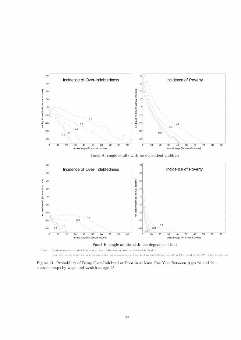
annual wage (% annual income)

net l

iqui

d w

ealth

(% a

nnua

l inc

ome)

0 10 20 30 40 50 60 70 80 90

-40

-30

-20

-10

0

10

20

30

40

0.9

0.3

0.1

Incidence of Over-Indebtedness

0.70.5

annual wage (% annual income)

net l

iqui

d w

ealth

(% a

nnua

l inc

ome)

0 10 20 30 40 50 60 70 80 90

-40

-30

-20

-10

0

10

20

30

40

0.9

0.30.1

Incidence of Poverty

Panel A: single adults with no dependent children

annual wage (% annual income)

net l

iqui

d w

ealth

(% a

nnua

l inc

ome)

0 10 20 30 40 50 60 70 80 90

-40

-30

-20

-10

0

10

20

30

40

0.9

0.30.1

Incidence of Over-Indebtedness

0.5

annual wage (% annual income)

net l

iqui

d w

ealth

(% a

nnua

l inc

ome)

0 10 20 30 40 50 60 70 80 90

-40

-30

-20

-10

0

10

20

30

40

0.90.3

0.1

Incidence of Poverty

Panel B: single adults with one dependent childN o t e s : C o n t o u r m ap s g e n e r a t e d f r om m o d e l , u s in g c a l ib r a t e d p a r am e t e r s r e p o r t e d in Ta b le 4

M o n e t a ry va lu e s e x p r e s s e d a s p e r c e n t a g e s o f av e r a g e a n nu a l g r o s s h o u s e h o ld in c om e b e tw e e n a g e s 2 0 a n d 6 4 , e q u a l t o £ 4 5 ,7 5 7 in th e s im u la t io n s

Figure 21: Probability of Being Over-Indebted or Poor in at least One Year Between Ages 25 and 29 —contour maps by wage and wealth at age 25

72

and B of Figure 21 indicates that the probability of over-indebtedness and poverty tend to be lower

for households with dependent children than those without, a conclusion that is not particular to

the pairwise comparison that is provided here (see Appendix D for further statistics). The result arises

because the tax and benefit system that is considered for analysis makes a larger adjustment in response

to the presence of a child than the increase in consumption needs that is implicit in the (McClement’s)

equivalence scale that is assumed for the preference structure. This observation is perhaps unsurprising

from a policy perspective, given the effort that has been made during the last decade to improve the

financial circumstances of households with dependent children. It is important to note, however, that

the result depends heavily upon the value judgements that are implicit in the assumed equivalence scale.

Different results would be obtained if the relative consumption needs of children in practice are higher

than their nutritional requirements upon which the McClements scale is based, or if take-up rates for

associated benefits were under 100%. Furthermore, in relation to the scatter plots reported in Figure

21, the fact that the model takes no account of financial circumstances in generating temporal dynamics

of demographics is likely to be particularly important for household with dependant children.

We conclude this subsection by considering the circumstances of households as they near state

pensionable age (65 in the simulations). State pensionable age is interesting with reference to the

rational agent model, because it is assumed that all unsecured debt must be repaid by this time. Hence,

as state pensionable age nears in the model, the maximum unsecured debt that a household may have

falls, from just under £31,000 at the beginning of age 55 to £7,100 at the beginning of age 64 (see Table

4 for full details). In these circumstances it seems reasonable to include repayment of the principal

when defining over-indebtedness:

A household is considered to be over-indebted if the interest charge on their unsecured loans,

plus the fraction of the principal that is inversely proportional to the number of years before

they reach retirement age exceed 25% of their total disposable income.

Figure 22 reports contour maps for the probability that a 60 year old household is over-indebted (as

it is redefined here) or impoverished (as it is defined in the preceding subsection) in any year between

ages 60 and 64. All four of the contour maps reported in Figure 22 describe very similar profiles,

suggesting a closer relation between the measures of poverty and over-indebtedness considered for 60

year olds, than those considered for 20 year olds in Figure 20. This is to be expected, given that

measures of indebtedness have a more immediate impact on consumption toward state pensionable age,

due to the assumption that all unsecured debt must be repaid by that time. Furthermore, individuals

are eligible for welfare benefits from age 60 that are worth almost twice the benefits that are provided

to childless households at age 20, which eliminates poverty for households with small debts and very

73

annual wage (% annual income)

net l

iqui

d w

ealth

(% a

nnua

l inc

ome)

0 10 20 30 40 50 60 70 80 90

-50

-40

-30

-20

-10

0

10

20

30

40

0.9

0.1

Incidence of Over-Indebtedness

0.30.5

annual wage (% annual income)

net l

iqui

d w

ealth

(% a

nnua

l inc

ome)

0 10 20 30 40 50 60 70 80 90

-50

-40

-30

-20

-10

0

10

20

30

40

0.9

0.1

Incidence of Poverty

0.3

Panel A: single adults

annual wage (% annual income)

net l

iqui

d w

ealth

(% a

nnua

l inc

ome)

0 10 20 30 40 50 60 70 80 90

-50

-40

-30

-20

-10

0

10

20

30

40

0.9

0.1

Incidence of Over-Indebtedness

0.3

annual wage (% annual income)

net l

iqui

d w

ealth

(% a

nnua

l inc

ome)

0 10 20 30 40 50 60 70 80 90

-50

-40

-30

-20

-10

0

10

20

30

40

0.9

0.1

Incidence of Poverty

0.3

Panel B: couplesN o t e s : C o n t o u r m ap s g e n e r a t e d f r om m o d e l , u s in g c a l ib r a t e d p a r am e t e r s r e p o r t e d in Ta b le 4

M o n e t a ry va lu e s e x p r e s s e d a s p e r c e n t a g e s o f av e r a g e a n nu a l g r o s s h o u s e h o ld in c om e b e tw e e n a g e s 2 0 a n d 6 4 , e q u a l t o £ 4 5 ,7 5 7 in th e s im u la t io n s

Figure 22: Probability of Being Over-Indebted or Poor in at least One Year Between Ages 60 and 64 —contour maps by wage and wealth at age 60

74

0

0.01

0.02

0.03

0.04

0.05

0.06

0.07

0.08

20 25 30 35 40 45 50 55 60 65age

prop

n of

pop

ulat

ion

over indebted equivalised consumption < £100 per w eek

Figure 23: Proportions of Population Over-Indebted / Credit Constrained by Age

low annual wages. This last observation highlights the practical importance of the welfare judgement

implicit in providing the pension guarantee from age 60.

8.3 The likelihood of becoming over-indebted when behaving rationally

To determine the likelihood of being constrained when behaving rationally, the current discussion is

based upon the cohort of 20,000 households that was generated by the rational agent model calibrated

to the full population (as discussed at length in Section 7). Analysis of this population revealed that

22% of generated households were over-indebted during at least one year of their simulated lives, and

that 19% chose to consume less than £100 per week (in equivalised terms) during at least one year

between the ages of 20 and 75. Furthermore, 1.4% of simulated households spent at least one year

during the working lifetime with less than £500 of available credit. These statistics indicate that credit

constraints play an important role in determining the consumption behaviour generated by our model,

which — in itself — is of little surprise.55 Of greater interest is the timing of the incidence of poverty and

over-indebtedness, and the reasoning behind observed events.

Figure 23 plots age profiles for the proportion of the simulated population identified as over-indebted,

and the proportion with equivalised consumption under £100 per week. The two age profiles reported

in the figure are very similar, which underscores the practical implications of over-indebtedness for

household consumption. The figure indicates that the incidence of over-indebtedness is highest at age

55As noted in Section 3.6, for example, the credit constraint explicitly determines consumption behaviour at the terminalage adopted for the model.

75

24, just prior to the birth of children in the model, and falls away rapidly after that age. In contrast,

the incidence of poverty (as it is defined above), rises sharply at age 25 and exceeds the incidence of

over-indebtedness until age 39, by which time the two series have converged.

The discrete fall in the proportion identified as over-indebted at age 25 is due to the higher welfare

benefits that are payable to households with dependent children. The coincident discrete rise in the

proportion of the population identified with low consumption highlights the fact that the assumed

definition for over-indebtedness makes no allowance for consumption needs. The observation that

over-indebtedness is concentrated in younger households is consistent with survey data, and reflects

the dis-proportionate influence of negative income shocks for the young. This is underscored by the

observation that, of those households identified as over-indebted, 74% had suffered a low wage offer in

the same year, and 13% had experienced a divorce at some time during the preceding five years. The

positive correlation of over-indebtedness with these shocks to personal circumstances is consistent with

associated empirical findings, as discussed in Section 2.

To explore the circumstances that underly the incidence of over-indebtedness and poverty reported

above, Figure 24 augments the contour maps reported in Figure 21 to include point markers that

indicate the circumstances of those simulated households falling within the domain displayed in the

respective graphs. Specifically, of the 20,000 households simulated for analysis, 4,681 were identified as

single adults at age 25, 4,384 of whom were identified with net liquid assets and annual wages below the

upper thresholds reported Panel A of Figure 24. Similarly, of the 1,198 households identified as single

adults with one dependent child at age 25, 1,136 are reported in Panel B of the figure.

Panel A of Figure 24 indicates that a sizeable proportion of single adults without dependent children

at age 25 in the model are exposed to a high probability of experiencing at least one year of over-

indebtedness and poverty between ages 25 and 29. Indeed, the bulk of the single and childless population

are concentrated in a region of net liquid wealth and annual wage that is associated with a 30%

probability of over-indebtedness and poverty, and many are exposed to much higher risk of both events.

In contrast, Panel B of the figure indicates that very few single adults aged 25 with one dependent child

are subject to an appreciable probability of over-indebtedness, and almost none are likely to experience

poverty within the 5 year horizon considered here. This should be seen in the context of the caveats

that are made in the preceding subsection.

Figure 25 extends the above analysis to 25 year old couples. 4,946 households are identified as 25

year old couples without dependants in the simulated cohort, and 2,679 are identified as couples with

one dependent child. In contrast to the case of singles, however, Figure 25 omits a sizeable share of

these sub-populations — 3,611 couples without dependent children are identified with net liquid wealth

and annual wage falling within the relevant figures, and 1,936 couples with one dependent child. The

76

Panel A: single adults with no dependent children

Panel B: single adults with one dependent childN o t e s : C o n t o u r m ap s g e n e r a t e d f r om m o d e l , u s in g c a l ib r a t e d p a r am e t e r s r e p o r t e d in Ta b le 4

M o n e t a ry va lu e s e x p r e s s e d a s p e r c e n t a g e s o f av e r a g e a n nu a l g r o s s h o u s e h o ld in c om e b e tw e e n a g e s 2 0 a n d 6 4 , e q u a l t o £ 4 5 ,7 5 7 in th e s im u la t io n s

Figure 24: Probability of Single Adults Being Over-Indebted or Poor in at least One Year BetweenAges 25 and 29 — contour maps by wage and wealth at age 25

77

Panel A: couples with no dependent children

Panel B: couples with one dependent childN o t e s : C o n t o u r m ap s g e n e r a t e d f r om m o d e l , u s in g c a l ib r a t e d p a r am e t e r s r e p o r t e d in Ta b le 4

M o n e t a ry va lu e s e x p r e s s e d a s p e r c e n t a g e s o f av e r a g e a n nu a l g r o s s h o u s e h o ld in c om e b e tw e e n a g e s 2 0 a n d 6 4 , e q u a l t o £ 4 5 ,7 5 7 in th e s im u la t io n s

Figure 25: Probability of Couples Being Over-Indebted or Poor in at least One Year Between Ages 25and 29 — contour maps by wage and wealth at age 25

78

sizeable proportions of the population subgroups that are omitted from Figure 25 emphasise the higher

incomes that couples are considered to earn in the rational agent model relative to singles, and provide

an intuitive pre-cursor to the observations that are reported here.

Couples in the rational agent model tend to be exposed to a low probability of being over-indebted

between ages 25 and 29, with the risk tending to zero with the addition of a dependent child. Further-

more, Panel A of figure 25 indicates that couples without a dependent child are also subject to a low risk

of poverty, relative to singles. In contrast to these observations, however, the risk of experiencing at least

one year of poverty between ages 25 and 29 appears to be higher amongst couples with one dependent

child than it is amongst singles. This observation is driven by the fact that the proportion adjustment

made by the tax system in response to a dependent child exceeds the adjustment in household needs

(as represented by the equivalence scale), by a wider margin for singles than for couples.

To better understand the behaviour of households that are critically indebted at some point in their

simulated lives, Figure 26 reports age profiles for the circumstances of households that were identified to

undertake equivalised consumption of less than £50 per week during at least one year of their simulated

working lifetime (ages 20-64), who comprise 1.1% of the simulated cohort. There are clear similarities

between the critically indebted households identified here, and the profiles for indebted households

more generally that are reported in Section 7, which suggests that the statistics reported there are not

driven primarily by the thresholds used to define the population subgroup. As discussed in Section 7,

all of the profiles reported in Figure 26 indicate that households which suffer sever deprivation in at

least one year of their working lives tend to have a life experience from the outset that differs from the

remainder of the simulated cohort. Net income starts out lower on average for the poorer subgroup,

and trends downward, resulting in a disparity with the remaining population that grows substantially

by age 30. The downward trend in income is mirrored by consumption, resulting in an “expenditure

crunch” around age 26-27 — just after the first year in which dependent children are considered to enter

the model. Thereafter, consumption and income both tend to rise, but at a less rapid rate than observed

for the remainder of the population.

Relative to income, consumption begins higher and trends down faster with age for the poor popula-

tion subgroup, resulting in negative net liquid wealth that grows faster in the early 20s and peaks at age

27. This relation is attributable to two important influences. First, at the beginning of the simulated

lifetime, a household with an unlucky draw may bet upon the likelihood of receiving better draws in the

future. As each subsequent draw also turns out to be poor, the household will revise its expectations

regarding lifetime income downward, and adjust its per-period consumption down accordingly. Second,

the steeply inclining interest rates assumed for unsecured debt discourage debt accumulation, particu-

79

larly for low income households. After age 30, net liquid wealth rises until retirement, but the poor on

average never manage to catch up to the savings accrued by the remainder of the population.

8.4 Summary

• The rational agent model implies that 22% of households should experience at least one year of

over-indebted during their lives, and that 19% should chose to consume less than £100 per week

(in equivalised terms) during at least one year between the ages of 20 and 75. Over-indebtedness

and financial deprivation cannot simply be dismissed as a product of poor financial planning.

• Over-indebtedness generated by the rational agent model peaks at 7% of the population at age

24, and poverty peaks at 6.5% of the population at age 26.

• The uncertainty associated with a wage offer, and the incidence of marital dissolution appear tobe principal drivers of over-indebtedness in the model.

• Singles have a higher probability than otherwise similar couples of experiencing poverty or be-coming over-indebted early in the simulated lifetime because they tend to have lower incomes on

average, and more tenuous employment opportunities.

• The probability of over-indebtedness and poverty tend to be lower for households with depen-dent children than those without. This result arises because the tax and benefit system that is

considered for analysis makes a larger adjustment in response to the presence of a child than the

increase in consumption needs implied by the assumed equivalence scale. This result — in contrast

with the empirical incidence of poverty in the population — should be seen in the context of the

modelling assumptions, which include 100% benefit takeup and a family formation process that

is independent of income.

• The rational agent model suggests that the Pension Guarantee is an effective policy tool forlimiting the incidence of poverty prior to State Pensionable Age.

9 Summary and Conclusions

Private sector indebtedness has grown substantially over the last decade, and is the subject of increasing

public concern. The accrual of private sector debt has, however, been undertaken in the context of an

historically benign economic environment, which complicates any evaluation of whether, and in what

ways, the recent financial decisions of households may have been imprudent. This report is designed to

shed some light on this issue by exploring the interactions between household savings and indebtedness

using an articulated and carefully calibrated rational agent model.

80

0

20

40

60

80

100

120

140

160

20 30 40 50 60

age

% a

nnua

l inc

ome

subgroup average eg 1 eg 2 total average

Net Income

0

10

20

30

40

50

60

70

80

20 30 40 50 60

age

% a

nnua

l inc

ome

subgroup average eg 1 eg 2 total population average

Consumption

-100

0

100

200

300

400

500

600

20 30 40 50 60

age

% a

nnua

l inc

ome

subgroup average eg 1 eg 2 total average

Net Liquid Assets

N o t e s : A u th o r c a l c u la t io n s b a s e d o n s im u la t e d p o p u la t io n w i t h l e s s t h a n £ 5 0 p e r w e e k c o n sum p t io n a t s om e a g e b e tw e e n 2 0 a n d 6 4

M o n e t a ry va lu e s e x p r e s s e d a s p e r c e n t a g e s o f av e r a g e a n nu a l g r o s s h o u s e h o ld in c om e b e tw e e n a g e s 2 0 a n d 6 4 , e q u a l t o £ 4 5 ,7 5 7 in th e s im u la t io n s

Figure 26: Life profiles of households constrained at age 30

81

The rational agent model considered for analysis assumes that individuals make sensible financial

decisions. Decisions regarding consumption and labour supply are considered to be made to take into

account the prevailing economic environment, and expectations regarding the future. In this context,

households take on unsecured debt when they expect their respective incomes to rise in the future, so

that debt is a positive mechanism which facilitates income smoothing over the lifecycle. Importantly,

the expectations assumed for decision making in the model are consistent with the processes that govern

the intertemporal variation. Furthermore, the rational agent model has been specifically designed to

capture key characteristics that have been identified by the empirical literature as having an important

influence on household saving and indebtedness.

The study obtains a number of interesting findings. First, the model that is described here substan-

tially under-states both non-pension wealth and unsecured debt reported for the private sector in the

National Accounts. With regard to the understatement of non-pension wealth, we conjecture that the

difference between the model and survey data could be resolved by including an explicit bequest motive

in the model. In the case of unsecured debt, however, plausible magnitudes for the effects of augmenting

the model to better reflect the complexity of the household’s asset allocation problem suggest that the

model would still understate the National Accounts aggregate by 30%. While this observation does not

permit any strong conclusions to be drawn, it does suggest the need for further analysis.

Second, unsecured debt generated by the rational agent model tends to arise as the product of low

incomes. Low incomes, as they bear upon debt, are found to arise as the primarily due to changes in

marital status (and marital dissolution in particular), and the (exogenously imposed) probability of a

low wage offer (included as a proxy for involuntary unemployment). These observations are qualita-

tively consistent with survey data, and emphasise the importance of “indirect drivers” of private sector

indebtedness. Indeed, to the extent that individuals are unable to affect the probability that they suffer

negative shocks of the type referred to here, one might consider there to exist a potential insurance role

for government.

Third, the model suggests that the trend toward a higher educated population should result in

greater demand for credit early in any given birth cohort’s lifetime, and larger debts for those who are

indebted. These effects are driven primarily by the higher wage growth with age that is commonly

observed for higher educated, relative to lower educated individuals. If this result is found to accurately

describe the practical reality in the future, then it may provide a motive to expand the role of student

loan programmes.

Fourth, the rational agent model implies that approximately one fifth of all households should

experience at least one year of over-indebted and poverty during their lives. Over-indebtedness and

financial deprivation are observed from the model to peak in the mid 20s, and levels just under 10%

82

of the respective birth cohort, and again are found to be driven primarily by the receipt of a low

wage offer or a marital dissolution. This result is important as it implies that over-indebtedness and

financial deprivation cannot simply be dismissed as a product of poor financial planning. Singles without

dependent children tend to have the highest probability of being over-indebted or experiencing a period

of low consumption. This is, in part, driven by the fact that the tax and benefit system considered for

analysis makes a larger adjustment in response to the presence of a dependent child than the coincident

increase assumed for consumption needs. This finding should be taken in the context of the modelling

assumptions which imply that all benefits are taken up and that lone parents are on average better off

than is observed empirically.

References

Antoniewicz, R., Bonci, R., Generale, A., Marchese, G., Neri, A., Maser, K. & OŠHagan, P. (2005),

Household Wealth: Comparing Micro and Macro Data in Canada, Italy and United States. Paper

prepared for Luxembourg Wealth Study Workshop, 27-29 January.

Attanasio, O., Low, H. & Sanchez-Marcos, V. (2005), ‘Female labor supply as insurance against idio-

syncratic risk’, Journal of the European Economic Association 3, 755—764.

Attanasio, O. P. & Weber, G. (1995), ‘Is consumption growth consistent with intertemporal optimiza-

tion?’, Journal of Political Economy 103, 1121—1157.

Auerbach, A. J. & Kotlikoff, L. J. (1987), Dynamic Fiscal Policy, Cambridge University Press, Cam-

bridge.

Balcer, Y. & Sadka, E. (1986), ‘Equivalence scales, horizontal equity and optimal taxation under utili-

tarianism’, Journal of Public Economics 29, 79—97.

Barsky, R. B., Kimball, M. S., Juster, F. T. & Shapiro, M. D. (1997), ‘Preference parameters and

behavioral heterogeneity: an experimental approach in the health and retirement survey’, Quarterly

Journal of Economics 112, 537—579.

Benito, A. (2007), Housing equity as a buffer: evidence from UK households. Bank of England Working

Paper, 324.

Benito, A. & Mumtaz, H. (2006), Consumption excess sensitivity, liquidity constraints and the collateral

role of housing. Bank of England Working Paper 306.

Blundell, R., Browning, M. & Meghir, C. (1994), ‘Consumer demand and the life cycle allocation of

household expenditure’, Review of Economic Studies 61, 57—80.

83

Blundell, R., Meghir, C. & Smith, S. (2002), ‘Pension incentives and the pattern of early retirement’,

Economic Journal 112, C153—C170.

Bridges, S. & Disney, R. (2004), ‘Use of credit and arrears on debt among low-income families in the

United Kingdom’, Fiscal Studies 25, 1—25.

Browning, M. & Crossley, T. F. (2001), ‘The life-cycle model of consumption and saving’, Journal of

Economic Perspectives 15, 3—22.

Bus, J. C. P. & Dekker, T. (1975), ‘Two efficient algorithms with guaranteed convergence for finding a

zero of a function’, ACM Trans. Math. Software 1, 330—345.

CAB (2003), Financial over-commitment survey. Research Study conducted on behalf of CAB by

MORI, July 2003.

Carroll, C. D. (2001), ‘A theory of the consumption function, with and without liquidity constraints’,

Journal of Economic Perspectives 15, 23—45.

Carroll, C. D. & Kimball, M. S. (1996), ‘On the concavity of the consumption function’, Econometrica

64, 981—992.

Carroll, C. D. & Kimball, M. S. (2001), Liquidity constraints and precautionary saving. NBERWorking

Paper 8496.

Cooley, T. F. & Prescott, E. C. (1995), Economic growth and business cycles, in T. F. Cooley, ed.,

‘Frontiers of Business Cycles Research’, Princeton University Press, Princeton.

Deaton, A. (1997), The Analysis of Household Surveys, John Hopkins University Press, Baltimore.

Deaton, A. & Muellbauer, J. (1980), Economics and Consumer Behavior, Cambridge University Press,

Cambridge.

DTI (2003), Fair, clear and competitive. Department for Trade and Industry White Paper.

DTI (2005), Over-indebtedness in Britain: a DTI report on the MORI financial services survey. DTI:

London.

Fagan, C. (2003), Working-time preferences and work-life balance in the EU: some policy considerations

for enhancing the quality of life. European Foundation for the Improvement of Living and Working

Conditions: Dublin.

Fernandez-Corugedo, E. (2002), Soft liquidity constraints and precautionary saving. Bank of England

Working Paper 158.

84

Fernandez-Villaverde, J. & Krueger, D. (2006), Consumption over the life cycle: facts from Consumer

Expenditure Survey Data. Working Paper, University of Pennsylvania.

French, E. (2005), ‘The effects of health, wealth, and wages on labour supply and retirement behaviour’,

Review of Economic Studies 72, 395—427.

Greene, W. H. (1997), Econometric Analysis, Third Edition, Prentice-Hall, London.

Gross, D. B. & Souleles, N. S. (2002), ‘Do liquidity constraints and interest rates matter for consumer

behaviour? Evidence from credit card data’, Quarterly Journal of Economics 16, 149—185.

Grossman, S. J. & Shiller, R. J. (1981), ‘The determinants of the variability of stock market prices’,

American Economic Review 71, 222—227.

Gustman, A. L. & Steinmeier, T. L. (2005), ‘The social security early entitlement age in a structural

model of retirement and wealth’, Journal of Public Economics 89, 441—464.

Hall, R. E. (1988), Intertemporal substitution in consumption. NBER Working Paper, W0720.

Hansen, P. & Singleton, K. (1983), ‘Stochastic consumption, risk aversion and the temporal behaviour

of asset returns’, Journal of Political Economy 91, 249—266.

Heckman, J. (1974), ‘Life cycle consumption and labor supply: an explanation of the relationship

between income and consumption over the life cycle’, American Economic Review 64, 188—194.

Hicks, J. R. (1939), Value and Capital, Clarendon Press, Oxford.

Johnston, J. & DiNardo, J. (1997), Econometric Methods, McGraw-Hill, London.

Kempson, E. (2002), Overindebtedness in Britain. Report to the Department of Industry and Trade.

Khoman, E. & Weale, M. (2006), ‘The UK savings gap’, National Institute Economic Review 198, 97—

111.

KPMG (2003), Debt crisis — an attempt to make ends meet or a frivolous approach to spending? Press

Notice describing survey carried out by YouGov on behalf of KPMG.

Low, H. (2005), ‘Self-insurance in a life-cycle model of labour supply and savings’, Review of Economic

Dynamics 8, 945—975.

Mankiw, N. G. (1985), ‘Consumer durables and the real interest rate’, Review of Economics and Sta-

tistics 62, 353—362.

85

Mankiw, N. G., Rotemberg, J. J. & Summers, L. H. (1985), ‘Intertemporal substitution in macroeco-

nomics’, Quarterly Journal of Economics 100, 225—251.

Marmot, M., Banks, J., Blundell, R., Lessof, C. & Nazroo, J. (2003), Health, wealth and lifestyles of

the older population in England, IFS, London.

McClements, L. (1977), ‘Equivalence scales for children’, Journal of Public Economics 8, 191—210.

Mehra, R. & Prescott, E. C. (1985), ‘The equity premium: a puzzle’, Journal of Monetary Economics

15, 145—161.

Muellbauer, J. & van de Ven, J. (2004), Estimating Equivalence Scales for Tax and Benefits Systems.

NIESR Working Paper, 229.

Nelissen, J. H. M. (1998), ‘Annual versus lifetime income redistribution by social security’, Journal of

Public Economics 68, 223—249.

Nickell, S. (2004), Household Debt, House Prices and Consumption Growth. Speech given at Bloomberg

in London (September).

Sefton, J. A. (2000), ‘A solution method for consumption decisions in a dynamic stochastic general

equilibrium model’, Journal of Economic Dynamics and Control 24, 1097—1119.

Sefton, J. & van de Ven, J. (2004), ‘Simulating household savings and labour supply: an application of

dynamic programming’, National Institute Economic Review 188, 56—72.

Sefton, J., van de Ven, J. & Weale, M. (2006), Means Testing Retirement Benefits: fostering equity or

discouraging savings? NIESR Discussion Paper 283.

Sefton, J., van de Ven, J. & Weale, M. (2007), Means testing retirement benefits: fostering equity or

discouraging savings? forthcoming in the Economic Journal.

Solomou, S. & Weale, M. (1997), ‘Personal sector wealth in the United Kingdom, 1920-56’, Review of

Income and Wealth 43, 297—318.

Stephens, M. (2006), ‘Paycheque receipt and the timing of consumption’, Economic Journal 116, 680—

701.

Stern, N. H. (1976), ‘On the specification of models of optimal income taxation’, Journal of Public

Economics 6, 123—162.

Taylor, M. F. (2005), British Household Panel Survey Users Manual. Colchester: University of Essex.

86

Tudela, M. & Young, G. (2003), ‘The distribution of unsecured debt in the United Kingdom: survey

evidence’, Bank of England Quarterly Bulletin 2003, 417—427.

Waldron, M. & Young, G. (2006), ‘The state of British household finances: results from the 2006 NMG

Research survey’, Bank of England Quarterly Bulletin 46, 397—403.

Zeldes, S. P. (1984), Optimal consumption with stochastic income. Ph.D. thesis, Masachusetts Institute

of Technology.

Zeldes, S. P. (1989a), ‘Consumption and liquidity constraints: an empirical investigation’, Journal of

Political Economy 97, 305—346.

Zeldes, S. P. (1989b), ‘Optimal consumption with stochastic income: deviations from certainty equiva-

lence’, Quarterly Journal of Economics 104, 275—298.

Ziliak, J. P. & Kniesner, T. J. (2005), ‘The effect of income taxation on consumption and labor supply’,

Journal of Labor Economics 23, 769—796.

87

A Household level data for assets and debt from the BritishHousehold Panel Survey

The British Household Panel Survey (BHPS) provides detailed panel data for households reported at

annual intervals between 1990/01 and 2004/05 (the most recent wave issued at the time of writing). The

original sample, comprised of 10264 interviewed individuals drawn from 5538 households, was selected

to be representative of the UK cross-sectional population in 1990/01.56 The data provided by wave 10

of the BHPS, for 2000/01, are of particular interest here as they include responses to a suite of questions

that were designed to describe household assets and debt.57 When combined with the time-series aspect

of the survey, these questions provide a valuable source of wealth data for the UK.

Wave 10 of the BHPS provides data for 8903 interviewed individuals from 4916 households. Including

additions made to the original BHPS sample expands the number of household records to 8761. This

sample was restricted for the current analysis to omit those households with self-employment income

in excess of 10 percent of labour income, or those with more than two adults, to give a total sample of

6975 households. Responses of these households were used to obtain three measures of household wealth

from the BHPS — housing wealth, securities wealth, and pension wealth. Each of these three measures

of wealth are described in the following subsections. The data were calculated using programmes that

are written for SPSS and GAUSS, which may be obtained from the authors upon request.

A.1 Housing wealth

Housing wealth refers to the value of a family’s place of residence (for owner occupiers), and their second

home (if they have one), net of any outstanding mortgage commitments.58 The illiquid nature of wealth

held in residential property complicates accurate evaluation for survey purposes. Various alternative

methods can be devised to impute an ‘expected’ or ‘reasonable’ value of housing wealth from alternative

data, such as the size of a household’s residence, its region, and the value at purchase. The BHPS places

the onus of such imputations upon the survey respondent by asking them: “About how much would

you expect to get for your home if you sold it today?” Similarly, with regard to the value of mortgage

debt the BHPS asked respondents: “Approximately how much is the total amount of your outstanding

loans on all the property you (or your household) own, including your current home?”

It is clear that answers to these sorts of questions may be inaccurate, which (in the case of aggregate

property value) the BHPS takes into consideration by asking respondents whether their expected value

56The first sample was drawn from the small users Postal Address file for Great Britain south of the Caledonian canal(excluding Northern Ireland). Due to the repeated survey methods employed, the most recent waves of the BHPS nolonger provide a representative sample of the UK population. See Taylor (2005) for further details regarding the BHPS.57The BHPS also includes wealth data for the 1985/86 wave, and is scheduled to provide similar data for 2005/06 in

2007.58Details are drawn from responses made by the household reference person (definition provided below).

88

falls into one of a specific range of values. The BHPS also asks whether the property is owned jointly

with a third party. Where shared ownership is identified (0.3 percent of respondents), 50 percent of the

property value was assigned to the household for the analysis presented here.

A.2 Securities wealth

Wave 10 of the BHPS asked respondents to provide information regarding the value of any savings

that they held in tradeable securities. Specific reference was made to the following: Savings or Deposit

Accounts; National Savings Bank (Post Office); TESSA or ISA; National Savings Certificates; Premium

Bonds; Unit Trusts / Investment Trusts; Personal Equity Plan; Shares (UK or foreign); National Savings

Bonds; or Government or company securities. Individuals were asked to reveal the value of their

aggregate savings in these products, and whether they were owned jointly or in their sole name. Where

joint holdings were identified, the analysis presented here assumes that 50 percent of the associated

value was owned by the responding individual.

Importantly, no explicit reference was made by interviewers to account statements or listed market

values. Rather, respondents are asked questions such as: “Thinking now about the investments you

have ... about how much is the total value of these investments?” The form of this question is consistent

with that asked for housing, and focusses upon perceived (rather than actual) household wealth.

The BHPS also asks respondents to provide details about any debts that they owe. With regard

to financial wealth, the relevant questions make specific reference to the following: Hire Purchase

Agreements; Personal Loans; Credit Cards; Catalogue or Mail Order Purchase Agreements; DSS Social

Fund loan; Overdrafts; Student Loan; any other loans for a private individual (not including mortgages).

The total value of assets and loans for a household were calculated by summing the individual

holdings recorded by the BHPS for any adult members of the household.

A.3 Pension wealth

Household wealth held in the form of pension entitlements is highly opaque in the UK, which has

resulted in a low level of public awareness regarding the provisions made for retirement and how such

provisions affect future standards of living. Nevertheless, pension savings have a prominent impact on

the circumstances of individuals over the life course, and should consequently be taken into consideration

in a study such as this.

In spite of their opacity, measures of pension wealth can be imputed using a series of variables that

are described by the BHPS. The methodology used here is similar to Blundell et al. (2002), and focuses

upon rules that were commonly applied by the various schemes from which the UK pension system

was comprised in 2000/01. Three pension schemes are considered for the imputation of pension wealth;

89

Occupational Pensions (OP), Personal Pensions (PP), and the State Earnings Related Pension Scheme

(SERPS). The basic state pension and the invalidity benefit, which are also addressed by Blundell et

al., are omitted here because they are treated separately in the tax and benefit routine of the simulation

model that is used for analysis.

The imputation method that was used to impute pension wealth involves two distinct stages. In

the first stage, the annuity associated with alternative pension entitlements was determined, and in the

second, the lifetime present value of the annuities identified in the first stage was calculated. Each of

these stages is discussed below.

Annuity value of pension entitlements

The BHPS data were first checked to determine whether an individual is identified as receiving a pension

in 2000/01. If so, then imputations are unnecessary, since the pension annuity is described explicitly

by the data (as a weekly benefit received). If, however, an individual is not identified as drawing upon

a retirement pension, then the value of their current entitlement to a future pension must be imputed.

Between 1978 and 2001, an individual could be a member of three alternative pension schemes that

relate retirement benefits to income earned during the working lifetime. Primarily, an individual could

choose to remain in SERPS, a State administered scheme, or to opt-out of the state system and instead

contribute to an OP and/or a PP.

The imputation procedure used to obtain the measures of pension wealth discussed here begins by

checking whether a given individual was employed in 2000/01, and if so, whether they were a member

of an OP and/or a PP. Individuals who are identified as contributing to an OP and/or a PP in 2000/01,

are assumed to have been members of their respective pension scheme(s) for the entire period during

which they were employed in the position held during 2000/01 (and hence to have opted out of SERPS).

The annuity associated with a 2000/01 entitlement to a future OP, AOP , is obtained by:

AOP = χ (PE2001 − βLEL2000)N (9)

where χ is the accrual rate (taking a value of 1/60 for employees in the private sector, and 1/80 for

employees in the public sector), PE2001 is the pensionable income (best salary for the period 1997-

2000 for employees in the private sector, and for the period 1990-2000 for the public sector), β is the

integration factor (equal to one for the private sector and zero for the public sector), LEL2000 is the

Lower Earning Limit associated with National Insurance Contributions (NICs) for 2000/01, and N is

the number of years of membership. Equation (9) is based upon the most common OP schemes that

were offered up to 2000/01, which took the form of Defined Benefit Plans.59 Since the BHPS provides

59See Blundell et al. (2002, p. C163).

90

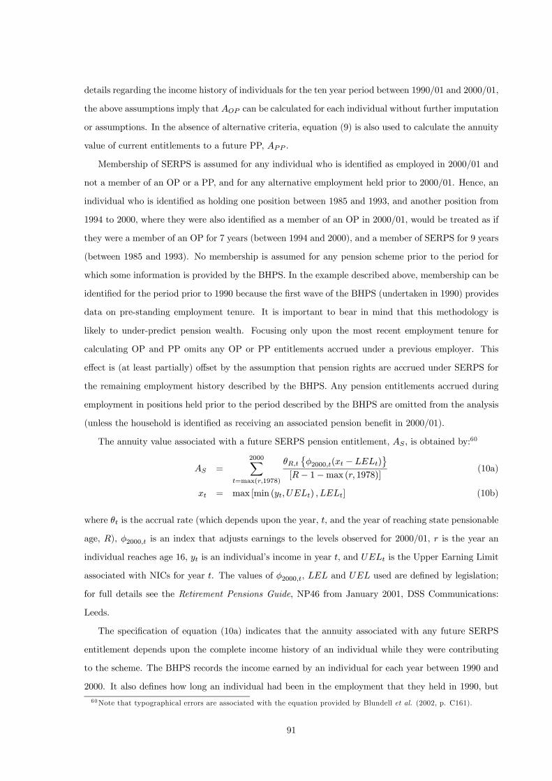
details regarding the income history of individuals for the ten year period between 1990/01 and 2000/01,

the above assumptions imply that AOP can be calculated for each individual without further imputation

or assumptions. In the absence of alternative criteria, equation (9) is also used to calculate the annuity

value of current entitlements to a future PP, APP .

Membership of SERPS is assumed for any individual who is identified as employed in 2000/01 and

not a member of an OP or a PP, and for any alternative employment held prior to 2000/01. Hence, an

individual who is identified as holding one position between 1985 and 1993, and another position from

1994 to 2000, where they were also identified as a member of an OP in 2000/01, would be treated as if

they were a member of an OP for 7 years (between 1994 and 2000), and a member of SERPS for 9 years

(between 1985 and 1993). No membership is assumed for any pension scheme prior to the period for

which some information is provided by the BHPS. In the example described above, membership can be

identified for the period prior to 1990 because the first wave of the BHPS (undertaken in 1990) provides

data on pre-standing employment tenure. It is important to bear in mind that this methodology is

likely to under-predict pension wealth. Focusing only upon the most recent employment tenure for

calculating OP and PP omits any OP or PP entitlements accrued under a previous employer. This

effect is (at least partially) offset by the assumption that pension rights are accrued under SERPS for

the remaining employment history described by the BHPS. Any pension entitlements accrued during

employment in positions held prior to the period described by the BHPS are omitted from the analysis

(unless the household is identified as receiving an associated pension benefit in 2000/01).

The annuity value associated with a future SERPS pension entitlement, AS , is obtained by:60

AS =2000X

t=max(r,1978)

θR,t©φ2000,t(xt − LELt)

ª[R− 1−max (r, 1978)] (10a)

xt = max [min (yt, UELt) , LELt] (10b)

where θt is the accrual rate (which depends upon the year, t, and the year of reaching state pensionable

age, R), φ2000,t is an index that adjusts earnings to the levels observed for 2000/01, r is the year an

individual reaches age 16, yt is an individual’s income in year t, and UELt is the Upper Earning Limit

associated with NICs for year t. The values of φ2000,t, LEL and UEL used are defined by legislation;

for full details see the Retirement Pensions Guide, NP46 from January 2001, DSS Communications:

Leeds.

The specification of equation (10a) indicates that the annuity associated with any future SERPS

entitlement depends upon the complete income history of an individual while they were contributing

to the scheme. The BHPS records the income earned by an individual for each year between 1990 and

2000. It also defines how long an individual had been in the employment that they held in 1990, but60Note that typographical errors are associated with the equation provided by Blundell et al. (2002, p. C161).

91

does not provide details regarding income earned prior to 1990. To identify the annuity value of SERPS

entitlements that were accrued prior to 1990, it is consequently necessary to impute measures of income.

Two equations of earnings by age were estimated to impute individual income prior to 1990, one for

higher educated (full-time education beyond the age of 18), and another for lower educated individuals.

The estimates were obtained using data for household reference people between ages 18 and 70 years,

as reported by the 2000/01 Family Expenditure Survey (1041 observations for the higher educated,

and 4476 for the lower educated subgroup). The earnings equations were estimated using a sample

selection model of individual full-time employment wages. This model takes into consideration the

fact that wages are only observed for individuals who are working, and that there is likely to be a

relationship between the probability of an individual working and their wage rate. The regressions were

undertaken using the “Sampsel” procedure in TSP; for full details refer to the “TSP 4.4 User’s Guide”

(see http://elsa.berkeley.edu/wp/tsp_user/tspugpdf.htm).

The sample selection model involves estimating two equations, a probit to identify individuals who

are employed, and a (log) wage equation:

empi = π0 + π1agei + π2age2i + π3mari + π4chu5i +

π5ch5pi + π6nai + π7totxi + ε1i (11)

ln(yi) = β0 + β1agei + β2age2i + β3age

3i + ε2i (12)

where: empi identifies when individual i( a 2 2 0+ a 2 2 1>3 0 ) works in excess of 30 hours per weekagei age of individual i( a 0 0 5 )

mari identifies when individual i is married(a 0 0 6= 1 o r 2 o r 3 )

chu5i number of children under 5 years old(a 0 4 0+ a 0 4 1 )

ch5pi number of children 5 years or older(a 0 4 2 )

nai the number of adults in i’s household(a 0 4 9 - ch u 5 - ch 5 p )

totxi total expenditure of i’s household(p 5 5 0 tp )

yi normal weekly wage of individual i( p 0 0 8+ p 0 1 1+ p 0 3 7+ p 0 4 7 )

Bracketed terms identify FES variable codes

Table 8 reports regression statistics derived for the sample selection model described above. These

statistics indicate that all of the estimated coefficients are highly significant. Two variables were omitted

from the regressions due to low statistical significance, one from each of the lower and higher educated

subgroups. The implied profiles of income with age are displayed in Figure 27.

In addition to the wage profiles obtained from the sample selection model, Figure 27 also displays

92

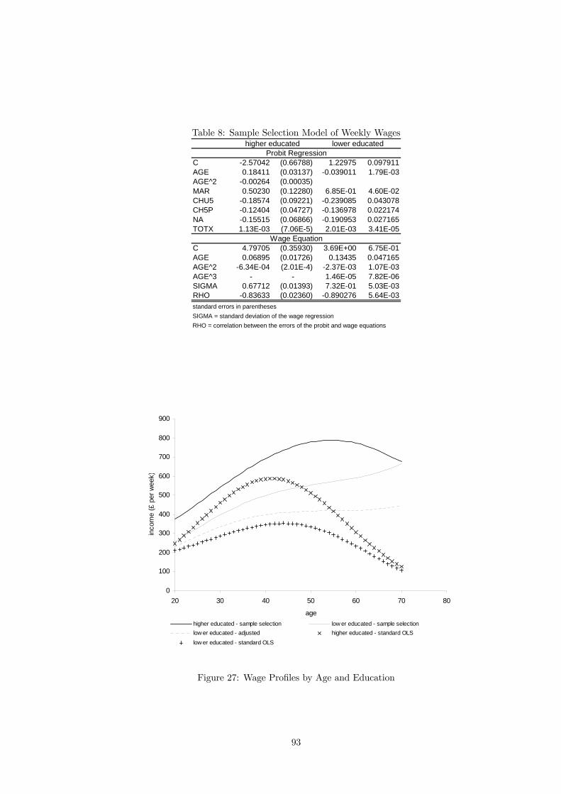
Table 8: Sample Selection Model of Weekly Wageshigher educated lower educated

Probit RegressionC -2.57042 (0.66788) 1.22975 0.097911AGE 0.18411 (0.03137) -0.039011 1.79E-03AGE^2 -0.00264 (0.00035)MAR 0.50230 (0.12280) 6.85E-01 4.60E-02CHU5 -0.18574 (0.09221) -0.239085 0.043078CH5P -0.12404 (0.04727) -0.136978 0.022174NA -0.15515 (0.06866) -0.190953 0.027165TOTX 1.13E-03 (7.06E-5) 2.01E-03 3.41E-05

Wage EquationC 4.79705 (0.35930) 3.69E+00 6.75E-01AGE 0.06895 (0.01726) 0.13435 0.047165AGE^2 -6.34E-04 (2.01E-4) -2.37E-03 1.07E-03AGE^3 - - 1.46E-05 7.82E-06SIGMA 0.67712 (0.01393) 7.32E-01 5.03E-03RHO -0.83633 (0.02360) -0.890276 5.64E-03standard errors in parenthesesSIGMA = standard deviation of the wage regressionRHO = correlation between the errors of the probit and wage equations

0

100

200

300

400

500

600

700

800

900

20 30 40 50 60 70 80

age

inco

me

(£ p

er w

eek)

higher educated - sample selection low er educated - sample selectionlow er educated - adjusted higher educated - standard OLSlow er educated - standard OLS

Figure 27: Wage Profiles by Age and Education

93

profiles estimated by standard Ordinary Least Squares (OLS). The profiles displayed in the figure indi-

cate that the adjustment for sample selection has a small effect on the estimates obtained at low ages

relative to high ages, which is consistent with the early retirement of individuals who had previously

earned relatively high incomes. The effect is, however, surprisingly large for the lower educated popula-

tion, a result that is attributable to the diminishing power of education as an identifier for the high wage

subgroup as age increases. Reducing the estimate obtained for β1 by 12 per cent of its standard error

alters the profile of wages for the lower educated subpopulation to the series denoted “lower educated

— adjusted” in Figure 27. The estimates derived from the sample selection model are used to project

incomes for the higher educated, while the adjusted profile is used for the lower educated.

In each year prior to 1990, an individual’s projected income, y, is given by:

yi,t =ρiy (agei,t)

φ2000,t(13a)

ρi =2000Xs=1990

yi,tφ2000,sy (agei,s)mi

(13b)

where yi,t is the income recorded by the BHPS for individual i in year t, y (agei,t) is the value of income

derived from equation (11), given the age of individual i in year t and the parameter values discussed

above, mi is equal to the number of years that yi,t > 0 between 1990 and 2000, and all other variables

take their previously stated definitions.

Given an individual’s age, education status and pension scheme contributions in 2000/01, and given

their labour force status and income history described by the BHPS, the procedures described above

enable the current annuity value of pension rights to be calculated.

Lifetime present value of pension annuities

The lifetime present value of the respective pension annuities described above, PWi, are calculated by:

PWi =

tuXt=2000

πt−2000δtAi (14)

where tu is the last year in which the household may receive pension annuity i, π is the real annual

growth rate of pension benefits (assumed to be 2 percent), δt is the probability that a household will

receive pension annuity i in year t, and Ai is the annuity value described in the previous subsection.

The probability that a household will receive a particular pension annuity in year t depends upon:

• the age of the person who accrued the pension rights in year t — it is assumed that all pensionrights will be received from state pensionable age (60 for women and 65 for men), if the BHPS

data do not indicate earlier receipt.

94

• the pension rights identified for an individual’s spouse — in the case of each of the three pensionschemes defined above the spouse is assumed to share pension entitlements if they are ineligible

for a pension of their own.

• the probability that an individual with a pension entitlement will survive up to a given year —assumed to depend upon their age and sex (based upon statistics reported for the period 2000-02

by the UK Government Actuaries Department).

B Simulated Tax and Benefits Policy

The simulations are based upon a parameterisation of the tax functions described in Section 3.2, which

were arrived at by the following procedure. First, for each practicable combination of numbers of adults

and children in a household, disposable (post-tax and benefit) income was identified as a function of

private (pre-tax and benefit) income. This function was then summarised by a four piece linear spline.

Intersections between the linear segments of the spline were smoothed to omit discontinuities in the

marginal tax rate.61 This produced a set of parameters that describe the tax function of each household

type, distinguished by the number and age of household members. The parameters so obtained were

themselves summarised as a function of the numbers of adults and children in a household, and these

summaries are used by the model to generate the effects of transfer policy. Examples of the functions

applied for analysis are reported below.

C Calibration Statistics for Education Specific Subgroups

D Additional ContourMaps of Over-Indebtedness and Poverty

61The linear segments were smoothed using a Boltzmann function, which produces a sigmoidal curve.

95

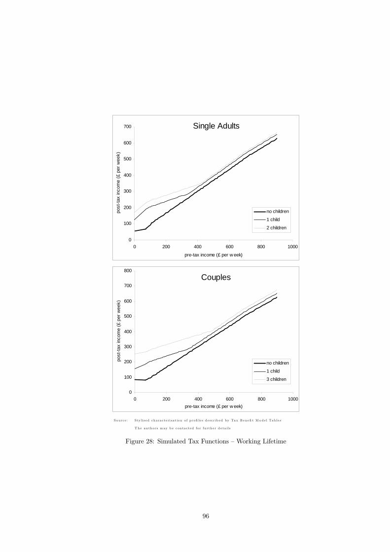
0

100

200

300

400

500

600

700

0 200 400 600 800 1000

pre-tax income (£ per w eek)

post

-tax

inco

me

(£ p

er w

eek)

no children

1 child

2 children

Single Adults

0

100

200

300

400

500

600

700

800

0 200 400 600 800 1000pre-tax income (£ per w eek)

post

-tax

inco

me

(£ p

er w

eek)

no children

1 child

3 children

Couples

S o u r c e : S ty l i s e d ch a r a c t e r i s a t io n o f p r o fi l e s d e s c r ib e d by Ta x B en efi t M o d e l Ta b le s

T h e a u th o r s m ay b e c o n ta c t e d fo r fu r t h e r d e t a i l s

Figure 28: Simulated Tax Functions — Working Lifetime

96

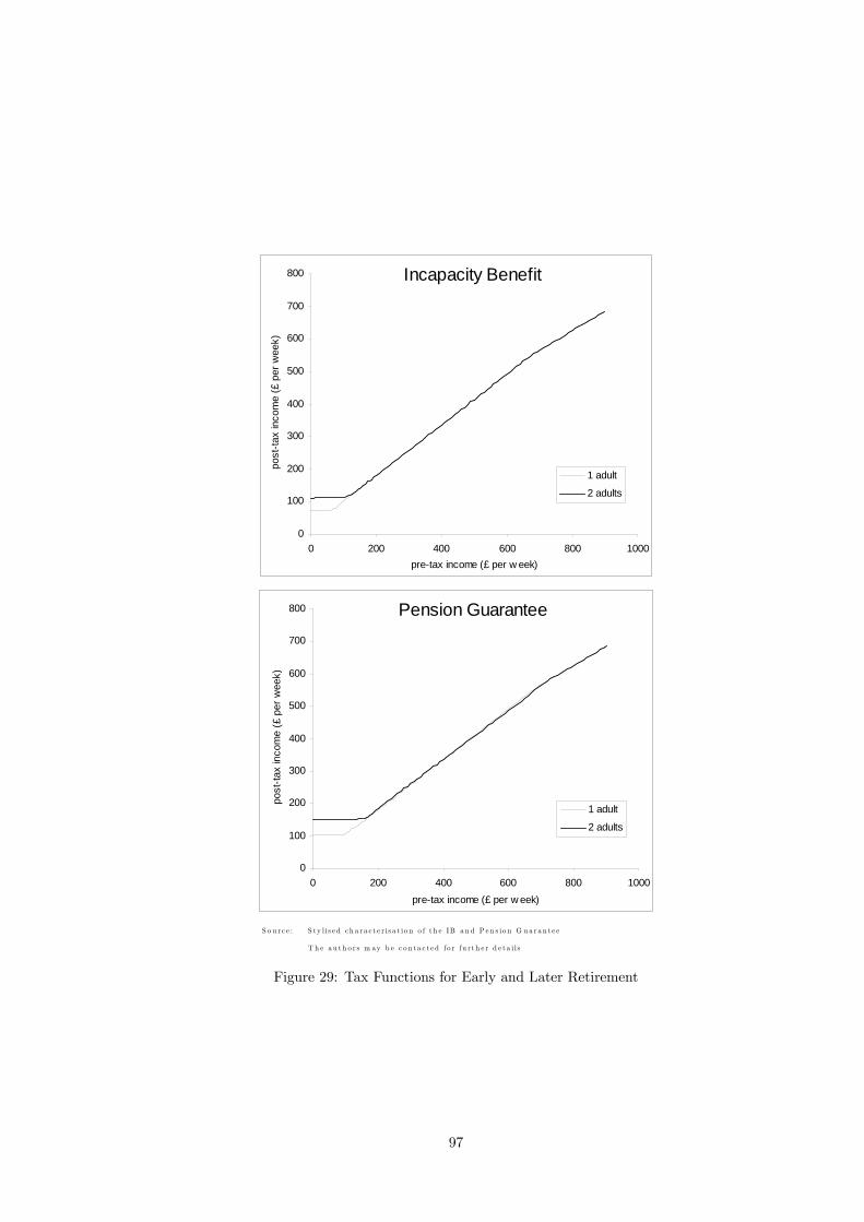
0

100

200

300

400

500

600

700

800

0 200 400 600 800 1000pre-tax income (£ per w eek)

post

-tax

inco

me

(£ p

er w

eek)

1 adult

2 adults

Incapacity Benefit

0

100

200

300

400

500

600

700

800

0 200 400 600 800 1000pre-tax income (£ per w eek)

post

-tax

inco

me

(£ p

er w

eek)

1 adult

2 adults

Pension Guarantee

S o u r c e : S ty l i s e d ch a r a c t e r i s a t io n o f t h e IB a n d P e n s io n G u a ra n t e e

T h e a u th o r s m ay b e c o n t a c t e d fo r fu r t h e r d e t a i l s

Figure 29: Tax Functions for Early and Later Retirement

97

0

100

200

300

400

500

600

700

800

900

0 200 400 600 800 1000

pre-tax income (£ per week)

post

-tax

inco

me

(£ p

er w

eek)

.

1 adult

2 adult

Figure 30: Tax Functions for Retirement

0

0.1

0.2

0.3

0.4

0.5

0.6

0.7

0.8

0.9

1

20 25 30 35 40 45 50 55 60 65

age

prop

ortio

n of

pop

ulat

ion

Sample statistics - couples Sample statistics - singles Simulated statistics

couples

singles

N o te s : S am p le s t a t i s t ic s — a g e p r o fi l e s c a lc u la t e d f r om E x p e n d it u r e a n d Fo o d S u rv e y d a t a , 2 0 0 1 / 0 2 , 2 0 0 2 / 0 3 , a n d 2 0 0 3 / 0 4

S im u la t e d s t a t i s t i c s — a g e p r ofi l e s g e n e r a t e d f r om m o d e l , u s in g c a l ib r a t e d p a r am e t e r s r e p o r t e d in Ta b le 4

E L SA — p e r c e n t a g e o f m e n a g e d 5 5 -5 9 e c o n om ic a l ly in a c t iv e by w ea lt h q u in t i l e , 2 0 0 2 / 0 3 w av e o f t h e E n g l i s h

L o n g i t u d in a l S tu d y o f A g in g , Ta b le 4A .1 2 , M a rm o t e t a l . ( 2 0 0 3 )

Figure 31: Timing of Retirement — simulated versus survey data for lower educated households

98

0

0.5

1

1.5

2

2.5

20 25 30 35 40 45 50 55 60 65age

prop

of f

ull-t

ime

empl

oym

ent i

ncom

e

Sample statistics - couples Sample statistics - s ingles Simulated statistics

Geometric Mean of Private Non-Property Income

singles

couples

0

0.2

0.4

0.6

0.8

1

20 25 30 35 40 45 50 55 60 65age

varia

nce

Variance of log Private Non-Property Incomesingles

0

0.1

0.2

0.3

0.4

0.5

0.6

20 25 30 35 40 45 50 55 60 65age

varia

nce

Simulated statistics Sample statistics

couples

N o t e s : S am p le s t a t i s t i c s — a g e p r ofi l e s c a l c u la t e d f r om E x p e n d i t u r e a n d Fo o d S u rve y d a t a , 2 0 0 3 / 0 4

S im u la t e d s t a t i s t ic s — a g e p r o fi l e s g e n e r a t e d f r om m o d e l , u s in g c a l ib r a t e d p a r am e t e r s r e p o r t e d in Tab le 4

M on e t a ry va lu e s r e p o r t e d a s p r o p o r t io n s o f ave r a g e a n nu a l fu l l - t im e em p loym en t in c om e fo r 2 0 0 3 / 0 4 , e q u a l t o £ 2 2 ,7 2 4

Figure 32: Private Non-Property Income Profiles by Age — simulated versus survey data for lowereducated households

99

0

0.5

1

1.5

2

20 25 30 35 40 45 50 55 60 65age

prop

of f

ull-t

ime

empl

oym

ent i

ncom

e

Sample statistics - couples Sample statistics - singles Simulated statistics

Geometric Mean of Disposable Non-Property Income

singles

couples

0

0.2

0.4

0.6

0.8

1

20 25 30 35 40 45 50 55 60 65age

varia

nce

Variance of log Disposable Non-Property Income

singles

`

00.20.40.60.8

11.21.4

20 25 30 35 40 45 50 55 60 65age

varia

nce

Simulated statistics Sample statistics

couples

N o t e s : S am p le s t a t i s t i c s — a g e p r ofi l e s c a l c u la t e d f r om E x p e n d i t u r e a n d Fo o d S u rve y d a t a , 2 0 0 3 / 0 4

S im u la t e d s t a t i s t ic s — a g e p r o fi l e s g e n e r a t e d f r om m o d e l , u s in g c a l ib r a t e d p a r am e t e r s r e p o r t e d in Tab le 4

M on e t a ry va lu e s r e p o r t e d a s p r o p o r t io n s o f ave r a g e a n nu a l fu l l - t im e em p loym en t in c om e fo r 2 0 0 3 / 0 4 , e q u a l t o £ 2 2 ,7 2 4

Figure 33: Disposable Non-Property Income Profiles by Age — simulated versus survey data for lowereducated households

100

0

0.2

0.4

0.6

0.8

1

1.2

1.4

1.6

20 30 40 50 60 70 80age

prop

of f

ull-t

ime

empl

oym

ent i

ncom

e

Sample statistics - couples Sample statistics - singles Simulated Statistics

Geometric Mean of Household Consumption

singles

couples

00.10.20.30.40.50.6

20 30 40 50 60 70 80age

varia

nce

Variance of log Consumption

singles

0

0.1

0.2

0.3

0.4

0.5

20 30 40 50 60 70 80age

varia

nce

Sample statistics Adjusted statistics

couples

N o t e s : S am p le s t a t i s t i c s — a g e p r ofi l e s c a l c u la t e d f r om E x p e n d i t u r e a n d Fo o d S u rve y d a t a , 2 0 0 3 / 0 4

S im u la t e d s t a t i s t ic s — a g e p r o fi l e s g e n e r a t e d f r om m o d e l , u s in g c a l ib r a t e d p a r am e t e r s r e p o r t e d in Tab le 4

M on e t a ry va lu e s r e p o r t e d a s p r o p o r t io n s o f ave r a g e a n nu a l fu l l - t im e em p loym en t in c om e in 2 0 0 3 / 0 4 , e q u a l t o £ 2 2 ,7 2 4

Figure 34: Consumption Profiles by Age — simulated versus survey data for lower educated households

101

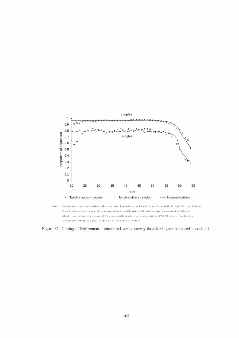
0

0.1

0.2

0.3

0.4

0.5

0.6

0.7

0.8

0.9

1

20 25 30 35 40 45 50 55 60 65

age

prop

ortio

n of

pop

ulat

ion

Sample statistics - couples Sample statistics - singles Simulated statistics

couples

singles

N o te s : S am p le s t a t i s t ic s — a g e p r o fi l e s c a lc u la t e d f r om E x p e n d it u r e a n d Fo o d S u rv e y d a t a , 2 0 0 1 / 0 2 , 2 0 0 2 / 0 3 , a n d 2 0 0 3 / 0 4

S im u la t e d s t a t i s t i c s — a g e p r ofi l e s g e n e r a t e d f r om m o d e l , u s in g c a l ib r a t e d p a r am e t e r s r e p o r t e d in Ta b le 4

E L SA — p e r c e n t a g e o f m e n a g e d 5 5 -5 9 e c o n om ic a l ly in a c t iv e by w ea lt h q u in t i l e , 2 0 0 2 / 0 3 w av e o f t h e E n g l i s h

L o n g i t u d in a l S tu d y o f A g in g , Ta b le 4A .1 2 , M a rm o t e t a l . ( 2 0 0 3 )

Figure 35: Timing of Retirement — simulated versus survey data for higher educated households

102

0

0.5

1

1.5

2

2.5

3

3.5

20 25 30 35 40 45 50 55 60 65age

prop

of f

ull-t

ime

empl

oym

ent i

ncom

e

Sample statistics - couples Sample statistics - singles Simulated statistics

Geometric Mean of Private Non-Property Income

singles

couple

0

0.5

1

1.5

2

20 25 30 35 40 45 50 55 60 65age

varia

nce

Variance of log Private Non-Property Incomesingles

0

0.2

0.4

0.6

0.8

1

20 25 30 35 40 45 50 55 60 65age

varia

nce

Simulated statistics Sample statistics

couples

N o t e s : S am p le s t a t i s t i c s — a g e p r ofi l e s c a l c u la t e d f r om E x p e n d i t u r e a n d Fo o d S u rve y d a t a , 2 0 0 3 / 0 4

S im u la t e d s t a t i s t ic s — a g e p r o fi l e s g e n e r a t e d f r om m o d e l , u s in g c a l ib r a t e d p a r am e t e r s r e p o r t e d in Tab le 4

M on e t a ry va lu e s r e p o r t e d a s p r o p o r t io n s o f ave r a g e a n nu a l fu l l - t im e em p loym en t in c om e fo r 2 0 0 3 / 0 4 , e q u a l t o £ 2 2 ,7 2 4

Figure 36: Private Non-Property Income Profiles by Age — simulated versus survey data for highereducated households

103

0

0.5

1

1.5

2

2.5

3

20 25 30 35 40 45 50 55 60 65age

prop

of f

ull-t

ime

empl

oym

ent i

ncom

e

Sample statistics - couples Sample statistics - singles Simulated statistics

Geometric Mean of Disposable Non-Property Income

singles

couples

00.20.40.60.8

11.2

20 25 30 35 40 45 50 55 60 65age

varia

nce

Variance of log Disposable Non-Property Income

singles

0

0.1

0.2

0.3

0.4

0.5

20 25 30 35 40 45 50 55 60 65age

varia

nce

Simulated statistics Sample statistics

couples

N o t e s : S am p le s t a t i s t i c s — a g e p r ofi l e s c a l c u la t e d f r om E x p e n d i t u r e a n d Fo o d S u rve y d a t a , 2 0 0 3 / 0 4

S im u la t e d s t a t i s t ic s — a g e p r o fi l e s g e n e r a t e d f r om m o d e l , u s in g c a l ib r a t e d p a r am e t e r s r e p o r t e d in Tab le 4

M on e t a ry va lu e s r e p o r t e d a s p r o p o r t io n s o f ave r a g e a n nu a l fu l l - t im e em p loym en t in c om e fo r 2 0 0 3 / 0 4 , e q u a l t o £ 2 2 ,7 2 4

Figure 37: Disposable Non-Property Income Profiles by Age — simulated versus survey data for highereducated households

104

0

0.5

1

1.5

2

2.5

20 30 40 50 60 70 80age

prop

of f

ull-t

ime

empl

oym

ent i

ncom

e

Sample statistics - couples Sample statistics - singles Simulated Statistics

Geometric Mean of Household Consumption

single

couples

00.10.20.30.40.50.60.7

20 30 40 50 60 70 80age

varia

nce

Variance of log Consumption

singles

0

0.1

0.2

0.3

0.4

0.5

20 30 40 50 60 70 80age

varia

nce

Sample statistics Adjusted statistics

couples

N o t e s : S am p le s t a t i s t i c s — a g e p r ofi l e s c a l c u la t e d f r om E x p e n d i t u r e a n d Fo o d S u rve y d a t a , 2 0 0 3 / 0 4

S im u la t e d s t a t i s t ic s — a g e p r o fi l e s g e n e r a t e d f r om m o d e l , u s in g c a l ib r a t e d p a r am e t e r s r e p o r t e d in Tab le 4

M on e t a ry va lu e s r e p o r t e d a s p r o p o r t io n s o f ave r a g e a n nu a l fu l l - t im e em p loym en t in c om e in 2 0 0 3 / 0 4 , e q u a l t o £ 2 2 ,7 2 4

Figure 38: Consumption Profiles by Age — simulated versus survey data for higher educated households

105

annual wage (% annual income)

net l

iqui

d w

ealth

(% a

nnua

l inc

ome)

0 10 20 30 40 50 60 70 80 90

-40

-30

-20

-10

0

10

20

30

40

0.9

0.3

0.1

Incidence of Over-Indebtedness

0.50.7

annual wage (% annual income)

net l

iqui

d w

ealth

(% a

nnua

l inc

ome)

0 10 20 30 40 50 60 70 80 90

-40

-30

-20

-10

0

10

20

30

40

0.9

0.30.1

Incidence of Poverty

0.5

Panel A: single adults with no dependent children

annual wage (% annual income)

net l

iqui

d w

ealth

(% a

nnua

l inc

ome)

0 10 20 30 40 50 60 70 80 90

-40

-30

-20

-10

0

10

20

30

40

0.90.3

0.1

Incidence of Over-Indebtedness

0.5

annual wage (% annual income)

net l

iqui

d w

ealth

(% a

nnua

l inc

ome)

0 10 20 30 40 50 60 70 80 90

-40

-30

-20

-10

0

10

20

30

40

0.9 0.30.1

Incidence of Poverty

Panel B: single adults with two dependent childrenN o te s : C o n t o u r m ap s g e n e r a t e d f r om m o d e l , u s in g c a l ib r a t e d p a r am e t e r s r e p o r t e d in Ta b le 4

Fo r h o u s e h o ld s w i t h 2 d e p e n d e n t ch i ld r e n : fi r s t ch i ld b o rn a t a g e 2 5 , s e c o n d ch i ld b o rn a t a g e 3 4

M o n e t a ry va lu e s e x p r e s s e d a s p e r c e n t a g e s o f av e r a g e a n nu a l g r o s s h o u s e h o ld in c om e b e tw e e n a g e s 2 0 a n d 6 4 , e q u a l t o £ 4 5 ,7 5 7 in th e s im u la t io n s

Figure 39: Probability of Being Over-Indebted or Poor in at least One Year Between Ages 34 and 39 —contour maps by wage and wealth at age 34

106

annual wage (% annual income)

net l

iqui

d w

ealth

(% a

nnua

l inc

ome)

0 10 20 30 40 50 60 70 80 90

-40

-30

-20

-10

0

10

20

30

40

0.90.3

0.1

Incidence of Over-Indebtedness

0.5

annual wage (% annual income)

net l

iqui

d w

ealth

(% a

nnua

l inc

ome)

0 10 20 30 40 50 60 70 80 90

-40

-30

-20

-10

0

10

20

30

40

0.9

0.3

0.1

Incidence of Poverty

0.5

Panel A: couples with no dependent children

annual wage (% annual income)

net l

iqui

d w

ealth

(% a

nnua

l inc

ome)

0 10 20 30 40 50 60 70 80 90

-40

-30

-20

-10

0

10

20

30

40

0.90.1

Incidence of Over-Indebtedness

annual wage (% annual income)

net l

iqui

d w

ealth

(% a

nnua

l inc

ome)

0 10 20 30 40 50 60 70 80 90

-40

-30

-20

-10

0

10

20

30

40

0.9

0.30.1

Incidence of Poverty

Panel B: couples with two dependent childrenN o te s : C o n t o u r m ap s g e n e r a t e d f r om m o d e l , u s in g c a l ib r a t e d p a r am e t e r s r e p o r t e d in Ta b le 4

Fo r h o u s e h o ld s w i t h 2 d e p e n d e n t ch i ld r e n : fi r s t ch i ld b o rn a t a g e 2 5 , s e c o n d ch i ld b o rn a t a g e 3 4

M o n e t a ry va lu e s e x p r e s s e d a s p e r c e n t a g e s o f av e r a g e a n nu a l g r o s s h o u s e h o ld in c om e b e tw e e n a g e s 2 0 a n d 6 4 , e q u a l t o £ 4 5 ,7 5 7 in th e s im u la t io n s

Figure 40: Probability of Being Over-Indebted or Poor in at least One Year Between Ages 34 and 39 —contour maps by wage and wealth at age 34

107