university of southampton research repository … of southampton abstract faculty of social and...

University of Southampton Research Repository

ePrints Soton

Copyright © and Moral Rights for this thesis are retained by the author and/or other copyright owners. A copy can be downloaded for personal non-commercial research or study, without prior permission or charge. This thesis cannot be reproduced or quoted extensively from without first obtaining permission in writing from the copyright holder/s. The content must not be changed in any way or sold commercially in any format or medium without the formal permission of the copyright holders.

When referring to this work, full bibliographic details including the author, title, awarding institution and date of the thesis must be given e.g.

AUTHOR (year of submission) "Full thesis title", University of Southampton, name of the University School or Department, PhD Thesis, pagination

http://eprints.soton.ac.uk

http://eprints.soton.ac.uk/

UNIVERSITY OF SOUTHAMPTON

Faculty of Social and Human Sciences

School of Mathematics

Screening experiments usingsupersaturated designs with application

to industry

by

Christopher James Marley

Thesis for the degree of Doctor ofPhilosophy

November 2010

UNIVERSITY OF SOUTHAMPTON

ABSTRACT

FACULTY OF SOCIAL AND HUMAN SCIENCES

SCHOOL OF MATHEMATICS

Doctor of Philosophy

SCREENING EXPERIMENTS USING SUPERSATURATED DESIGNS WITHAPPLICATION TO INDUSTRY

by Christopher James Marley

This thesis describes the statistical methodology behind a variety of industrialscreening experiments. The primary focus of the thesis is on supersaturated designsthat have more parameters to be investigated than runs available. Such designs areparticularly useful when experiments are expensive to perform. In addition, the sta-tistical issues behind a real-life screening experiment are investigated, where thereis a functional response and the factor levels cannot be set directly.

A study to compare several existing design and analysis methods for two-levelsupersaturated designs was carried out. A variety of different scenarios in terms ofnumbers of runs, numbers of factors and numbers of active factors were investigatedvia simulated experiments. The Gauss-Dantzig selector was identified as an effectiveanalysis method, whilst little difference was found in the practical performance ofdesigns from the different criteria. As a result of the study, several guidelines areprovided, to indicate when supersaturated designs are most likely to be effective asa screening tool.

A new criterion for designing supersaturated experiments under measures ofmulticollinearity is presented. The criterion is particularly applicable to experimentswhere factor levels cannot be set independently, although its application to two-leveldesigns is also demonstrated. An optimal allocation of factors to columns of anexisting design is also considered.

Supersaturated experiments are discussed in the context of robust product de-sign, where the interactions between control factors and noise factors are explored. Anew criterion specifically applicable to supersaturated robust product design experi-ments is described. The fact that the experimenter is interested in some parametersmore than others is exploited and the cost savings from using a supersaturated ex-periment are illustrated. It is demonstrated that substantial gains in power to detectactive effects can be achieved when using this new criterion.

Finally, the design and analysis of a practical screening experiment is discussed.Complicating features of the experiment include the multivariate nature of the re-sponse and the fact that factor levels cannot be set directly. A two-stage linearmixed effect model is applied, with principal components analysis used for the first-stage models. A novel method for finding follow-up runs to the screening experimentis described and implemented.

Contents

1 Introduction 1

2 A comparison of design and model selection methods for supersat-

urated experiments 5

2.1 Introduction . . . . . . . . . . . . . . . . . . . . . . . . . . . . . . . . 5

2.2 Design criteria and model selection methods . . . . . . . . . . . . . . 7

2.2.1 Design construction criteria . . . . . . . . . . . . . . . . . . . 7

2.2.2 Model selection methods . . . . . . . . . . . . . . . . . . . . . 8

2.3 Simulation Study and Results . . . . . . . . . . . . . . . . . . . . . . 12

2.3.1 Features varied in the simulation . . . . . . . . . . . . . . . . 12

2.3.2 Experiment simulation . . . . . . . . . . . . . . . . . . . . . . 14

2.3.3 Choice of tuning constants . . . . . . . . . . . . . . . . . . . . 14

2.3.4 Simulation results . . . . . . . . . . . . . . . . . . . . . . . . . 15

2.3.5 No active factors . . . . . . . . . . . . . . . . . . . . . . . . . 20

2.3.6 What is ‘effect sparsity’? . . . . . . . . . . . . . . . . . . . . . 21

2.4 Discussion . . . . . . . . . . . . . . . . . . . . . . . . . . . . . . . . . 23

3 Optimal supersaturated designs under measures of multicollinear-

ity with application to experiments where combinations of factor

levels cannot be set independently 25

3.1 Introduction . . . . . . . . . . . . . . . . . . . . . . . . . . . . . . . . 26

3.1.1 Background . . . . . . . . . . . . . . . . . . . . . . . . . . . . 26

i

3.1.2 Design selection criteria . . . . . . . . . . . . . . . . . . . . . 28

3.2 Using measures of multicollinearity to assign factors to columns in

existing designs . . . . . . . . . . . . . . . . . . . . . . . . . . . . . . 31

3.3 Combining νk(S) and the A-criterion . . . . . . . . . . . . . . . . . . 34

3.4 Generating supersaturated designs with independent combinations of

factor levels . . . . . . . . . . . . . . . . . . . . . . . . . . . . . . . . 37

3.4.1 Two-level designs using Criterion 4 . . . . . . . . . . . . . . . 38

3.4.2 Two-level designs using ν(c) . . . . . . . . . . . . . . . . . . . 40

3.4.3 Three-level designs . . . . . . . . . . . . . . . . . . . . . . . . 41

3.5 νA-optimal supersaturated designs where factor levels cannot be set

independently . . . . . . . . . . . . . . . . . . . . . . . . . . . . . . . 43

3.5.1 Example 1 . . . . . . . . . . . . . . . . . . . . . . . . . . . . . 43

3.5.2 Example 2 . . . . . . . . . . . . . . . . . . . . . . . . . . . . . 49

3.6 Discussion . . . . . . . . . . . . . . . . . . . . . . . . . . . . . . . . . 52

4 Supersaturated experiments for screening interaction effects with

application to robust product design 53

4.1 Introduction . . . . . . . . . . . . . . . . . . . . . . . . . . . . . . . . 54

4.2 Choosing supersaturated designs with control and noise factors . . . . 56

4.2.1 Criteria . . . . . . . . . . . . . . . . . . . . . . . . . . . . . . 56

4.3 Examples . . . . . . . . . . . . . . . . . . . . . . . . . . . . . . . . . 61

4.3.1 Example 1: 6 control and 4 noise factors . . . . . . . . . . . . 61



4.3.4 Other examples . . . . . . . . . . . . . . . . . . . . . . . . . . 74

4.4 Discussion . . . . . . . . . . . . . . . . . . . . . . . . . . . . . . . . . 76

ii

5 Advancing Tribology: Designed experiments to investigate the im-

pact of oil properties and process variables on friction 78

5.1 Introduction . . . . . . . . . . . . . . . . . . . . . . . . . . . . . . . . 78

5.2 Obtaining the data . . . . . . . . . . . . . . . . . . . . . . . . . . . . 82

5.2.1 The test procedure . . . . . . . . . . . . . . . . . . . . . . . . 82

5.2.2 Factors to be varied . . . . . . . . . . . . . . . . . . . . . . . . 82

5.2.3 Designed experiment . . . . . . . . . . . . . . . . . . . . . . . 85

5.3 Two-stage analysis of data . . . . . . . . . . . . . . . . . . . . . . . . 90

5.3.1 Using principal components analysis to model each observed

Stribeck curve . . . . . . . . . . . . . . . . . . . . . . . . . . . 90

5.3.2 How do the factors influence the Stribeck curves? . . . . . . . 91

5.3.3 Interpretation of the principal components . . . . . . . . . . . 97

5.4 Choosing follow-up runs . . . . . . . . . . . . . . . . . . . . . . . . . 100

5.4.1 Theory . . . . . . . . . . . . . . . . . . . . . . . . . . . . . . . 100

5.4.2 Experimental design for 10 follow-up runs . . . . . . . . . . . 102

5.5 Results of follow-up runs . . . . . . . . . . . . . . . . . . . . . . . . . 103

5.6 Discussion . . . . . . . . . . . . . . . . . . . . . . . . . . . . . . . . . 105

6 Overall conclusions and future work 110

6.1 Conclusions . . . . . . . . . . . . . . . . . . . . . . . . . . . . . . . . 110

6.2 Future work . . . . . . . . . . . . . . . . . . . . . . . . . . . . . . . . 112

References 114

iii

List of Figures

2.1 Proportion of times a given factor was wrongly declared inactive plot-

ted against ψ . . . . . . . . . . . . . . . . . . . . . . . . . . . . . . . 19

2.2 Performance measures, π1, . . . , π4, for the 22 18 experiment with µ =

5 using the Gauss-Dantzig selector for E(s2) (solid line) and Bayesian

D-optimal (dashed line) designs. . . . . . . . . . . . . . . . . . . . . . 21

2.3 Performance measures, π1, . . . , π4, for the 24 14 experiment with µ =

3 using the Gauss-Dantzig selector for E(s2) (solid line) and Bayesian

D-optimal (dashed line) designs. . . . . . . . . . . . . . . . . . . . . . 22

3.1 νcmax- (dashed line) and Acmax- (dotted line) efficiencies for designs

from the solvent candidate list with (w2, w3) = (0.5, 0.5) . . . . . . . . 47

3.2 νcmax (dashed line) and Acmax (dotted line) efficiencies for designs

from the solvent candidate list with (w2, w3) = (0.25, 0.75) . . . . . . 47

3.3 νcmax (dashed line) and Acmax (dotted line) efficiencies for designs

from the solvent candidate list with (w2, w3) = (0.75, 0.25) . . . . . . 48

3.4 νcmax (dashed line) and Acmax (dotted line) efficiencies for designs from

the Lubrizol compound candidate list with (w2, w3, w4) = (1/3, 1/3, 1/3) 50


the Lubrizol compound candidate list with (w2, w3, w4) = (0.5, 0.3, 0.2) 50





iv

5.1 Characteristic form of the Stribeck curve, showing how coefficient

of friction relates to speed, load and viscosity. Different lubrication

regimes are labeled. . . . . . . . . . . . . . . . . . . . . . . . . . . . . 79

5.2 Four example Stribeck curves obtained using different oils and differ-

ent settings of process variables . . . . . . . . . . . . . . . . . . . . . 80

5.3 Four example Stribeck curves (solid line) and their first-stage fits

(dashed line) . . . . . . . . . . . . . . . . . . . . . . . . . . . . . . . 92

5.4 QQ-plot of first-stage residuals for all 20 runs . . . . . . . . . . . . . 92

5.5 Profile plots for each of the four principal components, plotting βk

against δ for each of the k = 1, . . . , 91 parameters. . . . . . . . . . . . 94

5.6 Two Stribeck curves (solid line) and their second-stage fits (dashed

line) before the inclusion of the interaction of ZN APHOS with disc

roughness in the model . . . . . . . . . . . . . . . . . . . . . . . . . . 96

5.7 Four example Stribeck curves (solid line) and their second-stage fits

(dashed line) with approximate 95% confidence intervals (dotted lines). 96

5.8 QQ-plot of scaled second-stage residuals and plot of scaled second-

stage residuals against fitted values . . . . . . . . . . . . . . . . . . . 97

5.9 Plots of the first four principal components. . . . . . . . . . . . . . . 98

5.10 Plots illustrating the effect of a positive or negative loading on each

of the first four principal components . . . . . . . . . . . . . . . . . . 99

5.11 An observed Stribeck curve with a point of inflection. . . . . . . . . . 100

5.12 Plots of the first four principal components based on 20 (solid) and

29 (dashed) runs . . . . . . . . . . . . . . . . . . . . . . . . . . . . . 104

5.13 QQ-plot of scaled second-stage residuals and plot of scaled second-

stage residuals against fitted values based on 29 runs . . . . . . . . . 105

5.14 The effect of changing the level of Det MG from -0.99 to 1 on smooth

and rough discs. . . . . . . . . . . . . . . . . . . . . . . . . . . . . . . 106

5.15 The effect of changing the level of load from -1 to 1 on smooth and

rough discs. . . . . . . . . . . . . . . . . . . . . . . . . . . . . . . . . 106

v

5.16 The effect of changing the level of Disp B from -1 to 1 on smooth and

rough discs with high or low load. . . . . . . . . . . . . . . . . . . . . 107

5.17 Observed Stribeck curves for runs 1 and 2 (a and b) from the screening

stage (solid lines) and their repeats (dashed lines) . . . . . . . . . . . 108

5.18 Observed Stribeck curves from two validation runs (solid lines) and

their predicted curves (dashed lines) . . . . . . . . . . . . . . . . . . . 108

vi

List of Tables

2.1 Values of objective functions and maximum and minimum column

correlations for E(s2)-optimal and Bayesian D-optimal designs used

in the simulation study . . . . . . . . . . . . . . . . . . . . . . . . . . 13

2.2 Simulation study results for 22 18 designs . . . . . . . . . . . . . . . 16



2.5 Simulation results when there were no active factors . . . . . . . . . . 21

3.1 νf (6) for individual columns in the E(s2)-optimal design for 30 factors

in 18 runs . . . . . . . . . . . . . . . . . . . . . . . . . . . . . . . . . 33

3.2 Comparing performance of designs when the c factors with lowest

νf (c) are active (Scenario 1) and c factors with highest νf (c) are

active (Scenario 2) . . . . . . . . . . . . . . . . . . . . . . . . . . . . 34

3.3 Comparison of designs for 16 factors and 12 runs . . . . . . . . . . . 38



3.6 Design for 18 factors and 12 runs generated using Criterion 4 with

w4 = 1 and wV = 0.5 . . . . . . . . . . . . . . . . . . . . . . . . . . . 40

3.7 Comparison of three-level designs for 16 factors and 9 runs. . . . . . . 42

3.8 Three-level design for 16 factors and 9 runs generated using criterion

ν3A with wV = 0.1 . . . . . . . . . . . . . . . . . . . . . . . . . . . . . 42

3.9 Four solvents with 8 chemical properties from Ballistreri et al. (2002) 43

vii

3.10 Design for the solvent candidate list for (w2, w3) = (0.5, 0.5) and wV = 0 44

3.11 Design for the solvent candidate list for (w2, w3) = (0.5, 0.5) and

wV = 0.4 . . . . . . . . . . . . . . . . . . . . . . . . . . . . . . . . . . 44

3.12 Design for the solvent candidate list for (w2, w3) = (0.5, 0.5) and wV = 1 45

3.13 Comparison of designs for the solvent candidate list for (w2, w3) =

(0.5, 0.5) and wV = 0, 0.1, . . . , 0.9, 1 . . . . . . . . . . . . . . . . . . . 45

3.14 Comparison of designs for the Lubrizol compound candidate list for

(w2, w3, w4) = (1/3, 1/3, 1/3) and wV = 0, 0.1, . . . , 0.7, 0.8 . . . . . . . 51

3.15 Comparison of designs for the Lubrizol compound candidate list for

(w2, w3, w4) = (0.5, 0.3, 0.2) and wV = 0, 0.1, . . . , 0.7, 0.8 . . . . . . . . 51

4.1 Properties of 28-run designs for 6 control and 4 noise factors generated

using effect-focussed (E-F) E(s2)-, intercept-weighted (I-W) E(s2)-

and Bayesian D (B-D) -optimality . . . . . . . . . . . . . . . . . . . . 62

4.2 Number of active effects in each of 10 scenarios for the simulation

study for Example 1 . . . . . . . . . . . . . . . . . . . . . . . . . . . 63

4.3 Powers for various effects and Type I error rate for the 28-run design

for Example 1 generated using effect-focussed E(s2) with w = 6 . . . 65


for Example 1 generated using intercept-weighted E(s2) with w = 6 . 65


for Example 1 generated using Bayesian D-optimality with K = K1 . 66






4.8 Number of active effects in each of 10 scenarios for the simulation

study for Example 2 . . . . . . . . . . . . . . . . . . . . . . . . . . . 69

viii




for 4 Example 2 generated using intercept-weighted E(s2) with w = 4 70








4.14 Number of active effects in each of 8 scenarios for the simulation study

for Example 3 . . . . . . . . . . . . . . . . . . . . . . . . . . . . . . . 72




for Example 3 generated using intercept-weighted E(s2) with w = 4 . 73





5.1 Factors to be varied in the Stribeck curve experiment . . . . . . . . . 83

5.2 Characteristic values for eleven ingredients . . . . . . . . . . . . . . . 84

5.3 Minimum and maximum percentages of the eleven ingredients in the

oils . . . . . . . . . . . . . . . . . . . . . . . . . . . . . . . . . . . . . 86

5.4 Percentages of each ingredient and settings of the two process vari-

ables in the 20-run design . . . . . . . . . . . . . . . . . . . . . . . . 89

5.5 Design matrix for 20-run experiment . . . . . . . . . . . . . . . . . . 89

ix

5.6 Percentages of each ingredient and settings of the two process vari-

ables in the 10-run follow-up design . . . . . . . . . . . . . . . . . . . 102

5.7 Design matrix for 10-run follow-up experiment . . . . . . . . . . . . . 103

x

List of Accompanying Material

• CD containing a catalogue of effect-focussed E(s2) designs described in Chap-

ter 4. Control factors are denoted by capital letters and noise factors by lower

case letters.

xi

Declaration of authorship

I, Christopher Marley, declare that the thesis entitled Screening experiments

using supersaturated designs with application to industry and the work

presented in the thesis are both my own, and have been generated by me as the

result of my own original research. I confirm that:

• this work was done wholly or mainly while in candidature for a research degree

at this University;

• where any part of this thesis has previously been submitted for a degree or any

other qualification at this University or any other institution, this has been

clearly stated;

• where I have consulted the published work of others, this is always clearly

attributed;

• where I have quoted from the work of others, the source is always given. With

the exception of such quotations, this thesis is entirely my own work;

• I have acknowledged all main sources of help;

• where the thesis is based on work done by myself jointly with others, I have

made clear exactly what was done by others and what I have contributed

myself;

• parts of this work have been published as:

Marley, C.J. and Woods, D.C. (2010). A comparison of design and model

selection methods for supersaturated experiments. Computational Statistics

and Data Analysis, 54, 3158-3167.

Signed:

Date:

xii

Acknowledgments

I would like to thank my supervisor, Dr David Woods, and my advisor Professor

Susan Lewis, for their sustained guidance, enthusiasm and support throughout the

compilation of this thesis. I would also like to thank Professor Dennis Lin for his

encouragement and advice relating to Chapter 4 of this thesis, and also for his

kindness during my visit to Penn State. I am grateful for the funding from EPSRC

and acknowledge the generous support of the Lubrizol Corporation throughout my

PhD, in particular the assistance of Dr Andrew Rose, Dr Michael Gahagan, John

Durham, Dr Oliver Smith and Dr Robert Wilkinson with the case study in Chapter

5. Finally, thanks go to Dr John Fenlon for introducing me to the area of Design of

Experiments.

xiii

Chapter 1

Introduction

There are often many different variables, or factors which could potentially affect

the performance of a product or process. However, in reality, we expect only a small

number of these factors to have a substantive impact on the response(s) of interest.

This concept is known as effect sparsity (Box and Meyer, 1986). Screening is the

process of using designed experiments and statistical analysis to establish which of

these many factors have a substantive impact on the response(s) of interest.

Following the screening procedure, follow-up experiments involving fewer variables

are performed to enable the fitting of a more precise model and to validate the

findings at the screening stage (see for instance Meyer et al., 1996). This is more

cost effective than performing a much larger number of runs at the first stage, when

many more factors are under consideration.

The model used for screening experiments is typically of the form

Y = Xβ + ε ,

where Y is the response vector, X is a model matrix, β is a vector of unknown co-

efficients and ε is a vector of independent normally distributed random errors with

mean 0 and variance σ2. The model matrix X will typically only incorporate an

intercept and main effects, although sometimes two-factor interactions are investi-

gated. As such, experiments typically take place with the factors having two levels,

one high and one low, denoted by 1 and −1.

With a widening range of processes now under investigation in industry, and also an

1

increasing number of factors being explored as manufacturers look to improve the

quality of their products, the importance of effective screening strategies is greater

than ever.

Traditional methods of screening are full factorial and regular fractional factorial

experiments (see for instance Wu and Hamada, 2000, ch. 3-4). Full factorial ex-

periments are only utilised when the number of factors is small, since the number

of runs rapidly becomes large as the number of factors increases. When there are

a large number of factors, fractional factorial designs can result in very small and

efficient experiments but still with more runs than factors and complete aliasing

between effects potentially of interest.

Another method of screening is the use of non-regular fractions, where partial alias-

ing between some effects is present. Plackett-Burman designs (Plackett and Burman,

1946) are non-regular designs which can investigate up to m factors in m + 1 runs

when the number of runs is a multiple of 4. They have all main effects orthogo-

nal to each other, but partial aliasing between two-factor interactions occurs when

the number of runs is not a power of 2 (when the design corresponds to a regular

fraction).

Some experimenters use a group screening strategy, whereby the factors under inves-

tigation are partitioned into groups (Watson, 1961; Lewis and Dean, 2001). In each

experimental run, all factors within a group are set to the same level. Thus, factors

within the same group are completely confounded with each other at the screening

stage, with corresponding impact on confounding between interactions. This ap-

proach is most effective when the directions of the possible effects are known, with

only factors with the same directional effects being grouped together. For more

recent developments, including multi-stage group screening and group screening in-

volving interactions, see Morris (2006).

In this thesis we focus on the design and analysis of supersaturated experiments

(Booth and Cox, 1962; Lin, 1993; Wu, 1993). In certain experiments, particularly

in the manufacturing industry, the cost of a single run can be very high. Hence

there are very strict constraints on the number of runs that can be performed.

However, subject experts may produce a list of many factors which they think could

2

potentially affect the response under investigation. In order to investigate all of

these factors, the experimenter may wish to use a supersaturated design. This is

traditionally defined as a design which has fewer runs than factors to be investigated,

although a more general definition that there are more parameters of interest than

runs available is sometimes adopted. As a consequence, there are several challenging

issues involved in designing and analysing this type of experiment.

For a thorough review of screening strategies, see Dean and Lewis (2006).

When designing an experiment, our philosophy is that no effects of interest should

be completely confounded, that is, our design should provide some information on

all the parameters in the model. For supersaturated experiments we consider both

(i) how to design the experiment, including both design criteria and construction

methods, and

(ii) how to analyse the resulting data.

In addition, we provide guidance on the situations from which you are most likely

to see good performance from using a supersaturated experiment.

This thesis is structured as four independent contributing chapters, along with an

introduction and discussion chapter. The four contributing chapters are self con-

tained, with independent notation for each, and no cross-referencing between them.

Chapter 2 of this thesis compares different methods for the design and analysis of

supersaturated experiments. A new analysis method is also proposed and compared

to existing methods. Further to this, the performance of different sizes of supersat-

urated experiments under several scenarios, involving different numbers and sizes

of active effects, is investigated, enabling recommendations to be made on when

the practical implementation of supersaturated experiments is most likely to be

successful.

Chapter 3 describes a new class of criteria for designing supersaturated experiments.

This differs from most existing criteria in that it considers projections into subsets

of more than two factors. The criteria are used to generate several new two-level

supersaturated designs. Designs were also found for the case where factor levels

3

cannot be set independently, which has been little addressed in the literature. Such

a situation can occur when experimenting with chemical compounds. The new

set of criteria are particularly applicable to such an experiment, and examples are

presented to illustrate this. We also apply the criteria to assigning factors to columns

in existing supersaturated designs when some prior information is available.

Chapter 4 develops a new criterion for selecting supersaturated designs for robust

product design, exploiting interactions between control factors, which can be set

in the product specification, and noise factors, which cannot, but can be mimicked

in an experiment. Designs are generated and catalogued for many combinations of

control and noise factors. The benefits of these designs are illustrated by comparing

their performance against other designs in simulation studies.

Chapter 5 describes the design and analysis of a real screening experiment at the

specialty chemicals company Lubrizol. The experiment investigates the impact of oil

formulation and process variables on the friction between surfaces. The equipment

used is designed to mimic the friction and wear that may be experienced for instance

in an engine or gearbox. The output from each run of the experiment is a curve and

there are further statistical complications resulting from constraints on the design

space. A new method for choosing appropriate follow-up runs to the screening

experiment is described and implemented.

4

Chapter 2

A comparison of design and modelselection methods forsupersaturated experiments

Various design and model selection methods are available for supersaturated designs

having more factors than runs but little research is available on their comparison

and evaluation. Simulated experiments are used to evaluate the use of E(s2)-optimal

and Bayesian D-optimal designs and to compare four analysis strategies represent-

ing regression, shrinkage, orthogonal decomposition and a novel model averaging

procedure. Suggestions are made for choosing the values of the tuning constants for

each approach. Findings include that (i) the preferred analysis is via shrinkage; (ii)

designs with similar numbers of runs and factors can be effective for a considerable

number of active effects of only moderate size; and (iii) unbalanced designs can per-

form well. Some comments are made on the performance of the design and analysis

methods when effect sparsity does not hold.

2.1 Introduction

A screening experiment investigates a large number of factors to find those with a

substantial effect on the response of interest, that is, the active factors. If a large

experiment is infeasible, then using a supersaturated design in which the number of

factors exceeds the number of runs may be considered. This chapter investigates the

performance of a variety of design and model selection methods for supersaturated

experiments through simulation studies.

5

Supersaturated designs were first suggested by Box (1959) in the discussion of Sat-

terthwaite (1959). Booth and Cox (1962) provided the first systematic construction

method and made the columns of the design matrix as near orthogonal as pos-

sible through the E(s2) design selection criterion (see Section 2.2.1). Interest in

design construction was revived by Lin (1993) and Wu (1993), who developed meth-

ods based on Hadamard matrices. Recent theoretical results for E(s2)-optimal and

highly efficient designs include those of Nguyen and Cheng (2008). The most flexi-

ble design construction methods are algorithmic: Lin (1995), Nguyen (1996) and Li

and Wu (1997) constructed efficient designs for the E(s2) criterion. More recently,

Ryan and Bulutoglu (2007) provided a wide selection of designs that achieved lower

bounds on E(s2), and Jones et al. (2008) constructed designs using Bayesian D-

optimality. For a review of supersaturated designs, see Gilmour (2006).

The challenges in the analysis of data from supersaturated designs arise from cor-

relations between columns of the model matrix and the fact that the main effects

of all the factors cannot be estimated simultaneously. Methods to overcome these

problems include regression procedures, such as forward selection (Westfall et al.,

1998), stepwise and all-subsets regression (Abraham et al., 1999), shrinkage meth-

ods, including the Smoothly Clipped Absolute Deviation procedure (Li and Lin,

2002) and the Dantzig selector (Phoa et al., 2009), and orthogonal decomposition

methods (Georgiou, 2008). We compare the performances of one representative from

each of these classes of techniques, together with a new model-averaging procedure.

Strategies are suggested for choosing values of the tuning constants for each analy-

sis method. It is widely accepted that the effectiveness of supersaturated designs in

detecting active factors requires there being only a small number of such factors, a

principle known as effect sparsity (Box and Meyer, 1986).

Previous simulation studies compared either a small number of analysis methods

(Li and Lin, 2003; Phoa et al., 2009) or different designs (Allen and Bernshteyn,

2003), usually for a narrow range of settings. In our simulations, several settings are

explored with different numbers and sizes of active effects, and a variety of design

sizes. The results lead to guidance on when supersaturated designs are effective

screening tools.

6

In Section 2.2 we describe the design criteria and model selection methods investi-

gated in the simulation studies. Section 2.3 describes the studies and summarises

the results. Finally, in Section 2.4, we discuss the most interesting findings and draw

some conclusions about the effectiveness of the methods for different numbers and

sizes of active effects.

2.2 Design criteria and model selection methods

We consider a linear main effects model for the response

Y = Xβ + ε , (2.1)

where Y is the n × 1 response vector, X is an n × (m + 1) model matrix, β =

(β0, . . . , βm)T and ε is a vector of independent normally distributed random errors

with mean 0 and variance σ2. We assume that each of the m factors has two levels,

±1. The first column of X is 1n = [1, . . . , 1]T, with column i corresponding to the

levels of the (i− 1)th factor (i = 2, . . . ,m+ 1).

2.2.1 Design construction criteria

E(s2)-optimality

Booth and Cox (1962) proposed a criterion that selects a design by minimising the

sum of the squared inner products between columns i and j of X (i, j = 2, . . . ,m+

1; i 6= j). We extend this definition to include the inner product of the first column

with every other column of X to give

E(s2) =2

m(m+ 1)

∑i<j

s2ij , (2.2)

where sij is the ijth element of XTX (i, j = 1, . . . ,m + 1). The two definitions are

equivalent for balanced designs, that is, where each factor is set to +1 and -1 equally

often. The balanced E(s2)-optimal designs used in this chapter were found using the

algorithm of Ryan and Bulutoglu (2007). These designs achieve the lower bound on

7

E(s2) for balanced designs given by these authors and, where more than one design

satisfies the bound, a secondary criterion of minimising maxi<j s2ij is employed.

Bayesian D-optimality

Under a Bayesian paradigm with conjugate prior distributions for β and σ2 (O’Hagan

and Forster, 2004, ch. 11), the posterior variance-covariance matrix for β is pro-

portional to (XTX + K/τ 2)−1. Here, τ 2K−1 is proportional to the prior variance-

covariance matrix for β. Jones et al. (2008) suggested finding a supersaturated

design that maximises

φD = |XTX + K/τ 2|1/(m+1) .

They regarded the intercept β0 as a primary term with large prior variance, and

β1, . . . , βm as potential terms with small prior variances, see DuMouchel and Jones

(1994), and set

K =

(0 01×m

0m×1 Im×m

). (2.3)

The prior information can be viewed as equivalent to having sufficient additional runs

to allow estimation of all factor effects. This method can generate supersaturated

designs for any design size and any number of factors.

Bayesian D-optimal designs may be generated using a coordinate-exchange algo-

rithm (Meyer and Nachtsheim, 1995). The value of τ 2 reflects the quantity of prior

information; τ 2 = 1 was used to obtain the designs presented. An assessment (not

shown) of designs found for τ 2 = 0.2 and τ 2 = 5 indicated insensitivity of design

performance to τ 2; see also Jones et al. (2008).

2.2.2 Model selection methods

Four methods are examined: regression (forward selection), shrinkage (Gauss-Dantzig

selector), orthogonal decomposition (Singular Value Decomposition Principal Re-

gression Method; SVDPRM) and model averaging.

8

Forward selection

This procedure starts with the null model and adds the most significant factor main

effect at each step according to an F -test (Miller, 2002, pp. 39-42). The process

continues until the model is saturated or no further factors are significant. The

evidence required for the entry of a variable is controlled by the “F -to-enter” level,

denoted by α ∈ (0, 1).

Gauss-Dantzig selector

Shrinkage methods form a class of continuous variable selection techniques where

each coefficient βi is shrunk towards zero at a different rate. We investigate the

Dantzig selector, proposed by Candes and Tao (2007), in which the estimator β is

the solution to

minβ∈Rk||β||1 subject to ||XT(y −Xβ)||∞ ≤ δ . (2.4)

Here ||β||1 = |β0| + . . . + |βm| is the l1 norm, ||a||∞ = max(|a0|, . . . , |am|) is the

l∞ norm, and δ is a tuning constant. The Dantzig selector essentially finds the

most parsimonious estimator amongst all those that agree with the data. Optimi-

sation (2.4) may be reformulated as a linear program and solved, for example, using

the package lpSolve (Berkelaar, 2007) in R (R Development Core Team, 2009).

Candes and Tao (2007) also developed a two-stage estimation approach, the Gauss-

Dantzig selector, which reduces underestimation bias and was used for the analysis

of supersaturated designs by Phoa et al. (2009). First the Dantzig selector is used to

identify the active factors, and those factors whose coefficient estimates are greater

than γ are retained. Second, least-squares estimates are found by regressing the

response on the set of retained factors.

Singular Value Decomposition Principal Regression Method (SVDPRM)

Georgiou (2008) introduced the SVDPRM, based on an orthogonal decomposition

of a subset of the factor columns in X. The method has the following steps:

9

1. Retain the bn/2c factors with the largest absolute standardised contrasts and

use them to form a reduced model matrix Xr, where bac is the largest integer

below a.

2. Calculate the singular value decomposition of Xr:

Xr = UrDrVTr ,

where Xr is an n × (bn/2c + 1) matrix of rank t, Ur is an n × n orthogonal

matrix, Vr is an (bn/2c + 1) × (bn/2c + 1) orthonormal matrix, and Dr is

an n× (bn/2c+ 1) matrix containing the singular values. Dropping rows and

columns corresponding to zero singular values gives

Xt = UtDtVTt ,

where Xt, Ut, Dt and Vt are square t× t matrices and the columns of Ut are

the t left singular vectors.

3. Fit a linear main effects regression model with the t left singular vectors as

factors.

4. Transform the obtained coefficients back to the original variables and perform

F-tests to establish which are active.

By fitting a model in the orthogonal left singular vectors, we hope to obtain coeffi-

cients with smaller bias. Notice that this method can identify at most bn/2c active

factors. However, this is in line with the assumption of effect sparsity.

Model averaging

Here inference is based on a subset of models rather than on a single model. For

example, model-averaged coefficients are obtained by calculating estimates for a set

of models and then computing a weighted average where the weights represent the

plausibility of each model (Burnham and Anderson, 2002, ch. 4). This approach

provides more stable inference under repeated sampling from the same process.

10

For a supersaturated design, it is often not computationally feasible to include all

possible models in the procedure. Further, many models will be scientifically im-

plausible and therefore should be excluded (Madigan and Raftery, 1994). Effect

sparsity suggests restriction to a set of models each of which contains only a few fac-

tors. We propose a new iterative approach, motivated by the many-models method

of Holcomb et al. (2007).

1. Fit all models composed of two factors and the intercept and calculate for each

the value of the Bayesian Information Criterion (BIC)

BIC = n log((y −Xβ)T(y −Xβ)

n

)+ p log(n) , (2.5)

where p is the number of model terms.

2. For model i, calculate a weight

wi =exp(−0.5×∆BICi)∑K

k=1 exp(−0.5×∆BICk), i = 1, . . . , K ,

where ∆BICi = BICi − min1,...,K

(BICk) and K = m(m− 1)/2.

3. For each factor, sum the weights of those models containing the factor. Retain

the m1 < m factors with the highest summed weights. Parameter m1 should

be set fairly high to avoid discarding active factors.

4. Fit all possible models composed of three of the m1 factors and the intercept.

Calculate weights as in step 2. Retain the best m2 < m1 factors, as in step 3,

to eliminate models of low weight and obtain more reliable inference.

5. Fit all M models composed of m3 < m2 factors and the intercept, where

M = m2!/m3!(m2 −m3)!. Calculate new weights as in step 2.

6. Let β?1r, . . . , β

?m2r be the coefficients of the m2 factors in the rth model (r =

1, . . . ,M), where we set β?lr = 0 if the lth factor is not included in model r.

Calculate model-averaged coefficient estimates

11

β?l =

M∑r=1

wrβ?lr ,

where β?lr is the least-squares estimate of β?

lr if factor l is in model r, and 0

otherwise.

7. Use an approximate t-test, on n − m3 − 1 degrees of freedom, to decide if

each of the m2 factors is active. The test statistic is given by β?l /{Var(β?

l )}1/2,

where estimation of the model-averaged variance is given by

Var(β?l ) =

[M∑

r=1

wr

√Var(β?

lr) + (β?lr − β?

l )2

]2

,

and is discussed by Burnham and Anderson (2002, pp. 158-164).

The effectiveness of the each of the three methods described above depends on the

values chosen for the tuning constants, discussed in Section 2.3.3.

2.3 Simulation Study and Results

We identified a variety of features of a typical screening experiment and combined

these to provide settings of varying difficulty on which to test the design and model

selection methods.

2.3.1 Features varied in the simulation

• Ratio of factors to runs in the experiment. Three choices of increasing difficulty

were used and coded m n: 22 factors in 18 runs (22 18), 24 in 14 (24 14) and

26 in 12 (26 12).

• Design construction criteria. To investigate the use of E(s2)-optimal and

Bayesian D-optimal designs, one design was found for each m n under each

criterion. These designs were then used for all simulations with m factors and

n runs. For each design, the values of the objective functions E(s2) and φD are

12

given in Table 2.1, together with the maximum (ρmax) and minimum (ρmin)

correlations between factor columns.

For each m n, the designs have similar values of E(s2) and φD but different

structures. The E(s2)-optimal designs are balanced, whereas the Bayesian D-

optimal designs have 9, 7, and 5 unbalanced columns for the 22 18, 24 14 and

26 12 experiments respectively, with column sums of ±2. Also, the Bayesian

D-optimal designs have a wider range of column correlations than the E(s2)-

optimal designs. In particular, ρmax for an E(s2)-optimal design is always less

than or equal to that of the corresponding Bayesian D-optimal design.

• Number and sizes of active factors. The magnitude of the coefficient for each

of the c active factors was drawn at random from a N(µ, 0.2) for the following

scenarios.

1. Effect sparsity: c = 3, µ = 5.

2. Intermediate complexity: c = 4 or c = 5 (chosen with equal probability)

and µ = 4.

3. Larger number of small effects: c = 6 and µ = 3.

4. Larger number of effects of mixed size: c = 9 and one factor with each of

µ = 10, µ = 8, µ = 5, µ = 3, and five factors with µ = 2.

• Model selection methods. The four methods of Section 2.2.2 were applied and

tuning constants chosen as described in Section 2.3.3.

Table 2.1: Values of objective functions and maximum and minimum column cor-relations for E(s2)-optimal and Bayesian D-optimal designs used in the simulationstudy

Experiment 22 18 24 14 26 12Construction Criterion E(s2) D E(s2) D E(s2) DE(s2) 5.3 5.4 7.2 7.1 7.5 7.3φD 11.7 11.7 6.1 6.1 4.3 4.3ρmax 0.33 0.33 0.43 0.58 0.33 0.67ρmin 0.11 0 0.14 0 0 0

13

2.3.2 Experiment simulation

For each of 10,000 iterations:

1. From columns 2, . . . ,m+ 1 of X, c columns were assigned to active factors at

random.

2. To obtain the coefficients for the active factors, a sample of size c was drawn

from a N(µ, 0.2), and ± signs randomly allocated to each number.

3. Coefficients for the inactive factors were obtained as a random draw from a

N(0, 0.2).

4. Data were generated from model (2.1), with errors randomly drawn from a

N(0, 1), and analysed by each of the four model selection methods.

The random assignment of active factors to columns is important to remove selection

bias. The choice of distributions at steps 2 and 3 ensures separation between the

realised coefficients of the active and inactive factors.

2.3.3 Choice of tuning constants

For each method, a comparison of different values for the tuning constants was

carried out prior to the main simulation studies. The aim was to find values of the

tuning parameters that did not rely on detailed information from each simulation

setting. This was achieved either by choosing values to give robust performance

across the different settings, or by applying automated adaptive procedures.

Our strategy for the selection of δ and γ for the Gauss-Dantzig selector was to

control type II errors via δ, by choosing a larger than necessary model with the

Dantzig selector, and then control type I errors by choosing γ sufficiently large to

screen for spurious effects. To choose δ we used the standard BIC statistic (2.5)

which gave similar results to the use of AIC. Phoa et al. (2009) proposed a modified

AIC criterion which, in our study, consistently selected too few active effects when

c = 6. The value of γ needs to be sufficiently small so that few active factors are

declared inactive, but large enough for effects retained by the Dantzig selector to

14

be distinguishable from the random error. This was achieved by the choice γ = 1.5.

For Scenario 4, with µ = 2, an active effect may occasionally have magnitude less

than γ, resulting in slightly conservative results for the Gauss-Dantzig selector.

Model averaging is the most computationally demanding of the methods due to

the large number of regression models fitted. In the choice of m1, m2 and m3,

a balance must be struck between discarding potentially active factors too early

in the procedure, and including unlikely (for example, too large) models in the

final step. Preliminary studies showed that m1 = 18, m2 = 13 and m3 = 8 was

an effective compromise. In step 5 of the procedure, some models may not be

estimable. We found that removing a single factor overcame this problem. We

therefore chose to remove the factor with smallest weight that produced a non-

singular information matrix. Reassuringly, the power of the procedure to detect

active effects (see Section 2.3.4) is relatively robust to the values of m1 and m2.

Attempting to fit too large models in step 5, i.e. setting m3 too high, can result in

loss of power and also higher type I errors. We suggest that m3 is chosen broadly

in line with effect sparsity, and a little larger than the anticipated number of active

factors.

In forward selection, SVDPRM and model averaging, α = 0.05 was used based on

investigations (not presented) that showed α > 0.05 gave a substantial increase in

type I errors without a corresponding increase in power. Decreasing α resulted in

unacceptably low power for even the easiest simulation settings.

For each method studied, the results of the analysis can depend critically on the

choice of tuning constants. The Gauss-Dantzig selector has the advantages of having

a robust automated procedure for the choice of δ, and a straightforward interpre-

tation of γ as the minimum size of an active effect considered important enough to

detect. This quantity may often be elicited from subject experts (see, for example,

∆, in Lewis and Dean, 2001).

2.3.4 Simulation results

A factorial set of 96 simulations was run on the four features of Section 2.3.1. Four

different criteria were used to assess performance of the designs and analysis meth-

15

Table 2.2: Simulation study results for 22 18 designs. FS=forward selection,GDS=Gauss-Dantzig selector, SVD=SVDPRM, MA=model averaging; π1=power,π2=type I error rate, π3=coverage, π4=number of factors declared active

Design E(s2)-optimal Bayesian D-optimalAnalysis FS GDS SVD MA FS GDS SVD MAScenario 1: c = 3, µ = 5π1 1.00 1.00 1.00 1.00 1.00 1.00 1.00 1.00π2 0.11 0.01 0.05 0.02 0.11 0.03 0.05 0.02π3 1.00 1.00 1.00 1.00 1.00 1.00 1.00 1.00π4 5.07 3.17 3.99 3.41 5.07 3.61 3.97 3.42

Scenario 2: c = 4 or c = 5, µ = 4π1 0.89 1.00 0.97 0.99 0.90 1.00 0.97 0.99π2 0.09 0.01 0.04 0.02 0.10 0.04 0.04 0.02π3 0.85 0.99 0.92 0.98 0.86 0.99 0.92 0.98π4 5.57 4.72 5.06 4.74 5.69 5.11 5.04 4.74

Scenario 3: c = 6, µ = 3π1 0.57 0.93 0.86 0.90 0.58 0.95 0.86 0.89π2 0.06 0.02 0.03 0.02 0.06 0.04 0.03 0.02π3 0.37 0.77 0.60 0.74 0.38 0.82 0.60 0.73π4 4.35 5.97 5.68 5.63 4.43 6.26 5.68 5.62

Scenario 4: c = 9, µ = 10, 8, 5, 3, 2π1 0.56 0.73 0.47 0.55 0.56 0.75 0.47 0.56π1(10, 8) 1.00 1.00 1.00 1.00 1.00 1.00 1.00 1.00π1(5, 3) 0.78 0.92 0.64 0.80 0.78 0.93 0.64 0.80π1(2) 0.30 0.55 0.19 0.28 0.30 0.58 0.18 0.28π2 0.04 0.06 0.03 0.02 0.05 0.07 0.03 0.02π3 0.04 0.08 0.00 0.00 0.05 0.10 0.00 0.00π4 5.63 7.37 4.57 5.22 5.64 7.73 4.54 5.24

ods.

π1: Average proportion of active factors correctly identified (Power; larger-the-

better); for Scenario 4, the power was calculated separately for effects with

µ = 10, 8 (dominant; π1(10, 8)), µ = 5, 3 (moderate; π1(5, 3)) and µ = 2

(small; π1(2)).

π2: Average proportion of inactive factors which are declared active (Type I error

rate; smaller-the-better).

π3: Average proportion of simulations in which the set of factors declared active

included all those truly active (Coverage; larger-the-better).

16




Scenario 3: c = 6, µ = 3π1 0.31 0.61 0.38 0.46 0.30 0.65 0.40 0.46π2 0.08 0.09 0.03 0.09 0.08 0.09 0.03 0.09π3 0.02 0.20 0.04 0.11 0.02 0.26 0.05 0.10π4 3.22 5.23 2.84 4.29 3.16 5.57 2.93 4.31


π4: Average number of declared active factors.

The results are summarised in Tables 2.2, 2.3 and 2.4 for experiments 22 18, 24 14

and 26 12 respectively. These show that the Gauss-Dantzig selector has values of

π1 and π3 as high, or higher, than the other analysis methods in almost all the

simulations and often has very low values for π2. The Gauss-Dantzig selector was

found to have the most consistent performance of the three methods as measured

by the variances (not shown) of the proportions involved in π1, π2 and π3.

For the 22 18 experiment (Table 2.2), the performance of the Gauss-Dantzig selector

is almost matched by the model-averaging method for Scenarios 1–3. However, the

17




Scenario 3: c = 6, µ = 3π1 0.25 0.43 0.21 0.31 0.25 0.47 0.22 0.32π2 0.10 0.11 0.03 0.12 0.09 0.11 0.03 0.13π3 0.00 0.04 0.00 0.01 0.00 0.07 0.00 0.01π4 3.47 4.71 1.85 4.31 3.36 5.00 1.90 4.46


good performance of model averaging is not maintained for the more difficult 24 14

and 26 12 experiments. The addition of extra steps in the procedure, such as fitting

all four-factor models, may improve performance for larger numbers of factors at

the cost of more computation.

Forward selection has consistently the worst performance for Scenarios 1–3 measured

by π1 and π3, and also performs poorly under π2 for c = 3 and c = 4, 5. Also, the

type I error rate (π2) is often higher than the value set for the entry of a variable,

α = 0.05, due to the multiple testing. SVDPRM performs badly for Scenario 4,

which has a particularly large number of active factors. This poor performance is,

in part, due to the method being able to select at most bn/2c active factors.

18

●

●

●

●

●

●

●

●

●

●

●

●

●

●

●

●

●

●

●

●

●●

1.25 1.30 1.35 1.40 1.45 1.50 1.55

0.04

0.06

0.08

0.10

0.12

(a)

ψψ

Pro

port

ion

of ti

mes

a g

iven

fact

or is

dec

lare

d in

activ

e w

hen

it is

act

ive

●

●

●

●

●

●

●

●

●

●

●

●

●

●

●

●

●

●●

●

●

●

1.2 1.3 1.4 1.5 1.6

0.02

0.04

0.06

0.08

0.10

(b)

ψψ

Pro

port

ion

of ti

mes

a g

iven

fact

or is

dec

lare

d in

activ

e w

hen

it is

act

ive

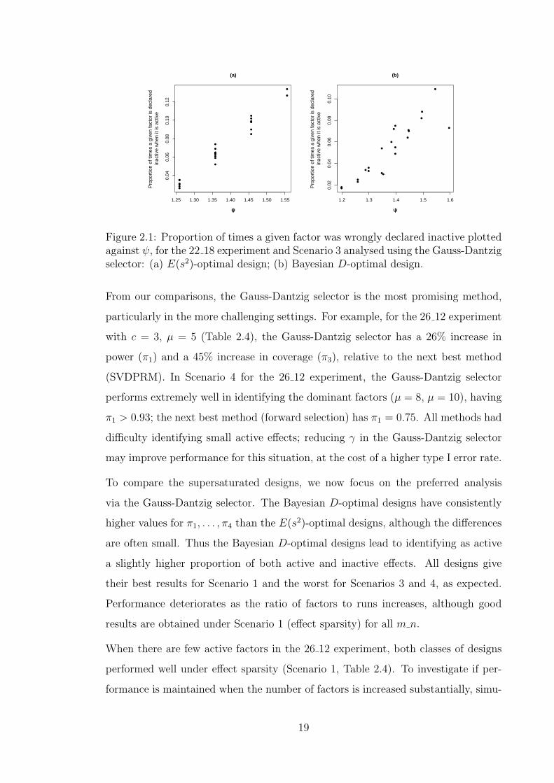
Figure 2.1: Proportion of times a given factor was wrongly declared inactive plottedagainst ψ, for the 22 18 experiment and Scenario 3 analysed using the Gauss-Dantzigselector: (a) E(s2)-optimal design; (b) Bayesian D-optimal design.

From our comparisons, the Gauss-Dantzig selector is the most promising method,

particularly in the more challenging settings. For example, for the 26 12 experiment

with c = 3, µ = 5 (Table 2.4), the Gauss-Dantzig selector has a 26% increase in

power (π1) and a 45% increase in coverage (π3), relative to the next best method

(SVDPRM). In Scenario 4 for the 26 12 experiment, the Gauss-Dantzig selector

performs extremely well in identifying the dominant factors (µ = 8, µ = 10), having

π1 > 0.93; the next best method (forward selection) has π1 = 0.75. All methods had

difficulty identifying small active effects; reducing γ in the Gauss-Dantzig selector

may improve performance for this situation, at the cost of a higher type I error rate.

To compare the supersaturated designs, we now focus on the preferred analysis

via the Gauss-Dantzig selector. The Bayesian D-optimal designs have consistently

higher values for π1, . . . , π4 than the E(s2)-optimal designs, although the differences

are often small. Thus the Bayesian D-optimal designs lead to identifying as active

a slightly higher proportion of both active and inactive effects. All designs give

their best results for Scenario 1 and the worst for Scenarios 3 and 4, as expected.

Performance deteriorates as the ratio of factors to runs increases, although good

results are obtained under Scenario 1 (effect sparsity) for all m n.

When there are few active factors in the 26 12 experiment, both classes of designs

performed well under effect sparsity (Scenario 1, Table 2.4). To investigate if per-

formance is maintained when the number of factors is increased substantially, simu-

19

lations of a 48 12 experiment were performed using each type of design. The results

indicated poor performance with π1 and π3 less than 0.61 and 0.37 respectively.

In practice, the assignment of active factors to the columns of a design may influence

the subsequent model selection. This was investigated by measuring the overall level

of correlation of a given column j of X by

ψj =m+1∑i=2

ρ2ij ,

where ρij is the correlation between columns i and j of X (i, j = 2, . . . ,m + 1).

Fig. 2.1 shows the proportion of times that a given factor was wrongly declared

inactive as a function of ψ for the 22 18 experiment and c = 6, µ = 3, analysed

using the Gauss-Dantzig selector. There are strong positive correlations for both the

E(s2)-optimal and Bayesian D-optimal designs, 0.98 and 0.90 respectively. Similar

trends were observed for other simulated experiments and scenarios (not shown).

This demonstrates the importance of using any prior information on the likely ac-

tivity of factors when assigning them to columns of the design. For the Bayesian

D-optimal design, any such information should ideally be incorporated in the design

construction through adjusting the elements of the matrix K in (2.3).

2.3.5 No active factors

Further simulations were used to check the performance of the design and analy-

sis methods when there are no active factors, a situation where π1 (power) and π3

(coverage) no longer apply. From Table 2.5, the Gauss-Dantzig selector is clearly

the best analysis method and rarely declares any factors active. The other meth-

ods have considerably higher type I errors, typically declaring at least two factors

active. Table 2.5 also shows that the E(s2)-optimal designs perform better than

the Bayesian D-optimal designs for the Gauss-Dantzig selector, agreeing with the

results for π2 in Section 2.3.4.

20

Table 2.5: Simulation results when there were no active factors. FS=forwardselection, GDS=Gauss-Dantzig selector, SVD=SVDPRM, MA=model averaging;π2=type I error rate, π4=number of factors declared active

Design E(s2)-optimal Bayesian D-optimalAnalysis FS GDS SVD MA FS GDS SVD MA22 18π2 0.11 0.01 0.19 0.05 0.12 0.03 0.19 0.05π4 2.52 0.12 4.15 1.13 2.55 0.57 4.11 1.14

24 14π2 0.12 0.01 0.10 0.08 0.12 0.02 0.10 0.08π4 2.88 0.23 2.40 1.85 2.82 0.43 2.47 1.88

26 12π2 0.13 0.01 0.07 0.10 0.12 0.02 0.07 0.11π4 3.28 0.33 1.74 2.64 3.22 0.52 1.81 2.83

2 4 6 8 10

0.4

0.6

0.8

1.0

Number of active factors

ππ 1

2 4 6 8 10

0.00

0.05

0.10

0.15

0.20


ππ 2

2 4 6 8 10

0.0

0.2

0.4

0.6

0.8

1.0


ππ 3

2 4 6 8 10

24

68

1012


ππ 4

Figure 2.2: Performance measures, π1, . . . , π4, for the 22 18 experiment with µ =5 using the Gauss-Dantzig selector for E(s2) (solid line) and Bayesian D-optimal(dashed line) designs.

2.3.6 What is ‘effect sparsity’?

A set of simulations was performed to assess how many active factors could be

identified reliably using supersaturated designs. These simulations kept the mean,

21

2 4 6 8 100.

40.

60.

81.

0


ππ 1

2 4 6 8 10

0.00

0.05

0.10

0.15

0.20


ππ 22 4 6 8 10

0.0

0.2

0.4

0.6

0.8

1.0


ππ 3

2 4 6 8 10

24

68

1012


ππ 4

Figure 2.3: Performance measures, π1, . . . , π4, for the 24 14 experiment with µ =3 using the Gauss-Dantzig selector for E(s2) (solid line) and Bayesian D-optimal(dashed line) designs.

µ, of an active factor constant and varied the number of active factors, c = 1, . . . , 10.

Fig. 2.2 shows the four performance measures for the 22 18 experiment with µ = 5

using the Gauss-Dantzig selector for analysis. Both the E(s2)-optimal and the

Bayesian D-optimal designs perform well for up to eight active factors. The Bayesian

D-optimal design has slightly higher π1, π2 and π3 values and thus tends to select

slightly larger models.

Fig. 2.3 shows the corresponding results for 24 14 experiment with µ = 3. The

performance, particularly under π1 and π3, declines more rapidly as the number

of active factors increases. Again, slightly larger models are selected using the

Bayesian D-optimal design, a difference which is not consistently observed for other

analysis methods. Further simulations (not shown) indicate considerable differences

in performance between settings where µ = 3 and µ = 5.

22

2.4 Discussion

The results in this chapter provide evidence that supersaturated designs may be a

useful tool for screening experiments, particularly marginally supersaturated designs

(where m is only slightly larger than n). They suggest the following guidelines for

the use of supersaturated designs.

1. The Gauss-Dantzig selector is the preferred model selection procedure out of

the methods investigated. If the design is only marginally supersaturated,

model averaging is also effective.

2. The ratio of factors to runs should be less than 2.

3. The number of runs should be at least three times the anticipated number of

active factors.

The simulations include situations where these conditions do not hold but neverthe-

less a supersaturated design performs well, for example, Table 2.4 Scenario 1 with

m/n > 2. However, evidence from our study suggests that 2 and 3 are conditions

under which supersaturated designs are most likely to be successful.

We notice that in Scenario 4 the assumption of effect sparsity is clearly violated, with

there being very many small active effects. However, the Gauss-Dantzig selector is

still very effective at picking out the largest effects.

With respect to guideline 3, we acknowledge that the experimenter will not know

the true number of active factors before performing the experiment. However, we

can use any available prior information about which factors may be active to guide

the choice of experiment size.

Little difference was found in the performance of the E(s2)-optimal and Bayesian

D-optimal designs, with the latter having slightly higher power to detect active

effects at the cost of a slightly higher type I error rate. The Bayesian D-optimal

designs may be preferred in practice, despite being unbalanced and having some high

column correlations, as follow-up experimentation may screen out spurious factors

23

but cannot detect active factors already removed. Such designs are readily available

in standard software such as SAS Proc Optex and JMP.

The simulations presented cover a broader range of conditions than previously con-

sidered and investigate more aspects of design performance. Further studies of in-

terest include incorporating interaction effects in the models, and Bayesian methods

of analysis, see for example Beattie et al. (2002).

24

Chapter 3

Optimal supersaturated designsunder measures ofmulticollinearity with applicationto experiments wherecombinations of factor levelscannot be set independently

Supersaturated designs may be defined as experimental plans with at least as many

factors as runs. Most existing criteria for generating or assessing supersaturated

designs focus only on dependencies between pairs of factors. We propose a new

class of criteria for supersaturated designs based on measures of multicollinearity

among subsets of the factors. Unlike some existing criteria, this new class can be

used to design experiments where factor levels cannot be set independently. We

apply the new criteria to two such experiments with a large list of possible design

points to choose from. We also generate new two- and three-level supersaturated

designs. The examples are used to demonstrate the benefits of the new methodology

and to illustrate some desirable properties of the resulting designs.

25

3.1 Introduction

3.1.1 Background

When performing experiments, there is often pressure to keep the number of runs

performed to a minimum, in order to reduce costs. In certain circumstances an

experimenter may wish to use a supersaturated design (SSD). Such designs have

more factors than runs. These designs are useful in screening situations, where the

experimenter initially wishes to determine which factors are ‘active’ (that is have a

large effect on the response of interest), rather than fitting a precise model. It is

widely accepted that the success of these designs in detecting the factors which have

a large impact on the response relies on the assumption of effect sparsity (Box and

Meyer, 1986).

There is much work in the literature on how to design two-level supersaturated

experiments. Booth and Cox (1962) proposed the popular E(s2) criterion, which

involves making the columns of the design matrix as near orthogonal as possible.

Lin (1993) proposed using half fractions of Hadamard matrices to construct SSDs,

whilst Wu (1993) supplemented Hadamard matrices with interaction columns. Wu

(1993) also briefly discussed A- and D-criteria which are extensions of classical

design optimality criteria that average over different models. Deng et al. (1996)

also discussed these ideas and proposed a new class of criteria, called B-optimality.

Nguyen (1996) found designs via algorithmic search using the E(s2) criterion, whilst

more recently Jones et al. (2008) used the coordinate exchange algorithm of Meyer

and Nachtsheim (1995) to generate designs based on Bayesian D-optimality.

There has also been interest in multi-level supersaturated experiments. Yamada

and Lin (1999) proposed the χ2 criterion and gave a construction method for three-

level SSDs. Chen and Liu (2008) and Liu and Lin (2009) proposed further methods

for constructing χ2-optimal mixed-level SSDs. Xu and Wu (2005) proposed the

generalised minimum aberration criterion for multi-level SSDs.

Most of the existing design criteria involve minimising dependencies between pairs

of columns. However, in even moderate sized experiments, it is quite possible that

there are more than two active factors. In order to achieve good projection properties

26

for the active factors, it is necessary to consider linear dependencies among more

than two factors. In this chapter we propose a new set of criteria incorporating

multicollinearity, and use this to generate two-level and multi-level designs.

Although there is much attention given to two-level and multi-level SSDs, there

is little work on cases where the levels of the factors cannot be set independently.

Such cases often occur in experimentation involving chemical compounds (see for

instance Put et al., 2004). The experimenter has a list of compounds which have

different properties. In this case, the properties are the factors in the experiment

and one compound must be chosen for each run of the experiment. Clearly, choosing

the compound fixes the levels of all the factors for this run and we have a different

design problem to the standard two-level or multi-level situation. We apply our new

set of criteria to such experiments and illustrate how its implementation can result

in designs with desirable properties.

Marley and Woods (2010) showed that, in practice, the choice of columns of the

design to which the active factors are assigned may have an impact on the power

to detect them. Xu and Wu (2005) suggested some designs with one column or-

thogonal to the rest, which can be useful if the experimenter believes one particular

factor is very likely to be active. More generally, Li et al. (2010) proposed a clus-

ter based method for assigning factors to columns when some prior information is

available. The current chapter provides a new method of factor to column assign-

ment and demonstrates its affect in existing Bayesian D-optimal and E(s2)-optimal

supersaturated designs.

The remainder of this chapter is organised as follows. In Section 3.1.2 we review

the concept of variance inflation factors (VIFs) for SSDs and propose a set of new

criteria for use in evaluating existing designs. In Section 3.2 we consider assignment

of factors to columns. Section 3.3 details a VIF based set of criteria which can be

used to generate new SSDs. Section 3.4 considers generating two-level and three-

level SSDs using the VIF based criterion to minimise multi-factor collinearity, whilst

Section 3.5 generates SSDs for cases where factor levels cannot be set independently.

Some discussion and concluding remarks are presented in Section 3.6.

27

3.1.2 Design selection criteria

Crosier (2000) stated that the multicollinearity of a set of variables cannot be es-

tablished from only their pairwise correlations. With supersaturated designs, the

aliasing schemes are often very complex, with factorial effects normally partially

aliased with several other effects. With this in mind, it makes sense to consider de-

pendencies amongst linear combinations of factors in the design and try to minimise

the impact of such relationships on the power to identify active factors.

Let X be a n×m design matrix. The (hj)th entry of X represents the level of factor

j for run h. One way of quantifying the linear dependencies amongst more than two

columns is to look at the variance inflation factors of X.

Consider first the non-supersaturated case. Then the variance inflation factor for

the kth variable (k = 1, . . . ,m) is defined as

νk = (1−R2k)−1 ,

where R2k is the R2 statistic when column k is regressed on all the other columns of

X and the intercept, that is

R2 = SSreg/SStot ,

where SSreg and SStot are respectively the regression sum of squares and the total

sum of squares from a regression of column k on all other columns.

The νk (k = 1, . . . ,m) can be interpreted as how much the variance of the kth

estimated regression coefficient is inflated as compared to when the columns of X

are not linearly related. Clearly lower VIFs imply less linear dependence among

columns in the design matrix.

Let ρij be the correlation between column i and column j of X and let the correlation

matrix for a given X be denoted by ρ = (ρij). Then

Result 1: The VIFs of a design can be expressed as the diagonal elements of the

inverse of the correlation matrix ρ (Neter et al., 1996, pp. 386).

28

Further, let X be the standardised design matrix (formed by columnwise subtraction

of the mean and dividing by the column standard deviation). Then

Result 2: The∑m

k=1 νk can be expressed in terms of eigenvalues of the information

matrix formed from the standardised design matrix X.

This can be shown as follows. The correlation matrix is ρ = X′X/n and the νk are

the diagonal elements of the inverse of the correlation matrix. So

m∑k=1

νk = tr

((X′X

n

)−1)= ntr((X

′X)−1)

Note that if A is an n× n symmetric matrix with r non-zero eigenvalues λ1, . . . , λr

then tr(A−) =∑r

i=1 λ−1i .

Hence

m∑k=1

νk = nm∑

k=1

λ−1k ,

where the λk are the eigenvalues of X′X.

Suppose that we calculate VIFs for subsets of size c of the columns in a given design.

For a given subset of columns, S, the variance inflation factor for the kth column in

the set S is then

νk(S) = (1−R2(k,S))−1 , (3.1)

where R2(k,S) is the R2 statistic when column k is regressed on all the other columns

in S and the intercept.

Under the assumption of effect sparsity, it is likely that only a small subset of the

factors in the experiment will be active. Therefore, it is desirable to have dependen-

cies among this subset of factors as low as possible to give good projection properties

of the design (i.e. the ability to estimate efficiently models containing a subset of

the factors), see for example Lin (1993). Hence νk(S) could prove a useful tool for

comparing existing SSDs or in a criterion for constructing new SSDs. An advan-

tage of using variance inflation factors is that not only pairwise dependencies are

evaluated, but also linear relationships involving more than two factors.

29

We initially propose two criteria for assessing and selecting designs. When evaluating

a design based on νk(S), we can calculate the average of the νk(S) across all subsets

of columns of size c, that is

Criterion 1: minimise ν(c) =1

cm′

m′∑l=1

c∑k=1

νk(Sl) ,

where Sl is the lth subset of columns of size c (l = 1, . . . ,m′) and

m′ = m!/c!(m− c)!.

Similarly, we could also consider the maximum νk(S) of a design.

Criterion 2: minimise ν(c) = maxl=1,...,m′; k=1,...,c

νk(Sl)

The idea of averaging νk(S) across different subsets is similar in principal to a set

of criteria proposed by Deng et al. (1996). They stated that there is a problem with

the widely used E(s2) criterion in that it provides no measurement of multi-factor

orthogonality. They proposed a new set of criteria, based on the regression sum of

squares, called B-optimality to deal with this problem, concentrating on producing

near orthogonal projections onto the set of (possibly greater than two) active factors.

The function they proposed is

Vc(X) =1

m′

∑|S|=c

vg(XS) ,

where

vg(XS) =∑k∈S

β′S−k(X′S−kXS−k)gβS−k .

XS is a n×c sub-matrix of design matrix X, XS−k is a n×(c−1) matrix corresponding

to S without k, xk is a column corresponding to the kth unit in S and βS−k =

(X′S−kXS−k)−1X′S−kxk.

They consider the cases g = 2, 1, 0 to give different penalties on near singularity.

The B1 criterion (where g = 1) is equivalent to Criterion 1 for two-level balanced

30

designs. Deng et al. (1996) only used the B-criteria to assess existing designs, and

did not generate any new designs.

3.2 Using measures of multicollinearity to assign

factors to columns in existing designs

We now show how measures of multicollinearity can be used to aid the assignment

of factors to columns within the designs. Marley and Woods (2010) show that the

assignment of active factors to columns of the design could greatly influence the

power to detect them in the analysis. If some prior information is available about

which factors are more likely to be active, then we may wish to assign these factors

to ‘good’ columns of the design, so that we are less likely to miss them.

Here we consider ranking columns of a design in order of their average VIFs. We

define the average VIF for column f based on subsets of size c as

νf (c) =1

cm′

m

cm′m∑

l=1

νf (Sl) ,

where Sl is the lth subset of columns of size c which contain column f ; l = 1, . . . , cm′

m,

and νf (Sl) is defined in equation (3.1).

The ranking of the columns may change depending on the value of c. We recommend

ranking with c = n/3. This is in line with a guideline proposed by Marley and Woods

(2010), who demonstrated that when using a two-level SSD, an experimenter could

reasonably expect to be able to detect up to n/3 active factors. They also showed

that performance of SSDs was much better when there were a smaller number of

active factors. Hence, ranking with c = n/3 corresponds to assigning factors to

columns based on a worst-case scenario in terms of the number of active factors that

might reasonably be detected. We consider assigning factors to columns in existing

designs generated under two different criteria; E(s2)-optimality and Bayesian D-

optimality.

Nguyen (1996) used an algorithm to construct SSDs using the E(s2) criterion, which

minimises the sum of the squared inner-products between columns i and j of X

31

(i, j = 1, . . . ,m).

E(s2) =2

m(m− 1)

∑i<j

s2ij ,

where sij is the ijth element of X′X. Notice how the E(s2) criterion only incorpo-

rates pairwise dependencies between the columns.

Jones et al. (2008) use Bayesian D-optimality as a criterion for generating SSDs.

In the Bayesian approach, the prior information can be viewed as equating to extra

runs in the experiment. Model uncertainty is incorporated through the choice of

prior. The parameter τ 2 reflects how much prior information we have. The aim is

to choose X to maximise

φD = |[1|X]′[1|X] + K/τ 2| , (3.2)

where 1 is a column of 1s and K is the prior dispersion matrix:

K =

(0 01×m

0m×1 Im×m

).

As an example of how designs can have very different average VIFs for different

columns, Table 3.1 shows νf (6) for all columns for Nguyen’s E(s2)-optimal design

for 30 factors in 18 runs. We notice a 16% inflation in variance for column 10, which

has the lowest average VIF, compared to a 28% inflation in variance for column 21,

which has the highest.

To illustrate the difference in performance of this design and several others, when

active factors are assigned to columns with low νf (c) compared with when they are

assigned to columns with high νf (c), we carry out a small simulation study. We

consider Bayesian D-optimal and E(s2)-optimal designs of four different sizes from

Jones et al. (2008) and Nguyen (1996) and different numbers of active factors. Two

different scenarios are considered for each design;

• Scenario 1: The c factors with lowest νf (c) are active

• Scenario 2: The c factors with the highest νf (c) are active.

32

Table 3.1: νf (6) for individual columns in the E(s2)-optimal design for 30 factorsin 18 runs

Column νf Column νf

1 1.192 16 1.2742 1.169 17 1.2213 1.272 18 1.1934 1.218 19 1.2725 1.194 20 1.2396 1.225 21 1.2767 1.220 22 1.2458 1.219 23 1.2479 1.214 24 1.18910 1.163 25 1.16911 1.240 26 1.21712 1.165 27 1.18513 1.221 28 1.22014 1.187 29 1.21615 1.190 30 1.189

We used c = n/3 for all designs except those for 24 factors in 12 runs. This is

because, for the design with 24 factors, there were some subsets of four factors for

which the VIFs could not be estimated. The simulation operated as follows:

1. Coefficients for active factors were simulated from a N(4, 0.2) distribution with

their sign chosen randomly.

2. Coefficients for inactive factors were simulated from a N(0, 0.2) distribution.

3. Errors, ε, were simulated from a N(0, 1) distribution.

4. Responses, Y were generated according to the model Y = Xβ + ε, where X

is the design matrix and β = β1, . . . , βm is the vector of coefficients.

5. The data were analysed using the Gauss-Dantzig selector (Candes and Tao,

2007) and the process repeated 2000 times.

Simulating active factors from a N(4, 0.2) distribution means that their coefficients

should be comfortably distinguishable from noise (signal to noise ratio = 4). The

Gauss-Dantzig selector was shown by Phoa et al. (2009) and Marley and Woods

33

Table 3.2: Comparing performance of designs when the c factors with lowest νf (c)are active (Scenario 1) and c factors with highest νf (c) are active (Scenario 2).Power1 and Power2 are the proportion of active factors correctly identified underScenarios 1 and 2. Similarly for Type I error rate1 and Type I error rate2.

Design Runs Factors c minf νf (c) maxf νf (c) Power1 Type I Power2 Type Icriterion error rate1 error rate2

Bayesian D-opt. 12 16 4 1.095 1.314 0.82 0.07 0.61 0.07E(s2)-opt. 12 16 4 1.092 1.202 1.00 0.02 0.73 0.09Bayesian D-opt. 12 18 4 1.141 1.261 0.89 0.06 0.76 0.08E(s2)-opt. 12 18 4 1.141 1.264 0.85 0.08 0.78 0.09Bayesian D-opt. 12 24 3 1.111 1.281 0.81 0.07 0.57 0.07E(s2)-opt. 12 24 3 1.110 1.173 0.99 0.03 0.89 0.05Bayesian D-opt. 18 30 6 1.157 1.288 0.98 0.04 0.86 0.08E(s2)-opt. 18 30 6 1.163 1.276 0.93 0.05 0.78 0.08

(2010) to be a promising analysis method for SSDs and hence we use it for the

analysis of data from the simulation study, using the tuning parameters detailed in

Marley and Woods (2010).

The results are summarised in Table 3.2. Under Scenario 2, the proportion of active

factors that we correctly identify (Power2) is always lower than that under Scenario

1 (Power1). Also, Type I error rate2 is always at least as big as Type I error rate1.

Both these points indicate worse performance when factors with higher νf (c) are

active. For instance, consider the E(s2)-optimal design for 30 factors in 18 runs.

We see that Power2 is 0.78 for this design, which compares rather poorly to a value

of 0.93 for Power1 for the same design. Similarly, the Type I error rate is much

higher for Scenario 2 (0.08) than for Scenario 1 (0.04). For the Bayesian D-optimal

design for 24 factors the difference in power between the two scenarios is even more

dramatic (0.81 for Scenario 1 compared to 0.57 for Scenario 2). These trends are

apparent across all the designs considered. We conclude that using prior information

to assign factors to columns of the design matrix using νf (c) as a criterion may have

considerable impact on the success of the screening experiment.

3.3 Combining νk(S) and the A-criterion

Although the application of Criterion 1 will result in a design with good projection

properties, in general the designs produced will have sub-optimal accuracy in param-

eter estimation. In particular, for very unbalanced designs, we can achieve excellent

34

projection properties at the price of high variances for parameter estimates. Here

we describe how to combine ν(c) with another criterion in order to achieve better

quality estimates of the parameters.

In Section 3.1.2 it was shown that for the non-supersaturated case

m∑k=1

νk = nm∑

k=1

λ−1k .

This can easily be extended to the supersaturated case. For a given subset, S, of c

columns we have

c∑k=1

νk(S) = nc∑

k=1

λ−1k (S) ,

where the λk(S) are the eigenvalues of X′SXS , where XS is the standardised design

sub-matrix for the columns corresponding to the columns in S.

Now, notice that for two-level balanced designs, X = X, since the column means of

X are all 0 and standard deviations are all 1. Hence,

Result 3: For two-level balanced designs, for each S,∑c

k=1 νk(S) is equivalent to

the A-optimality objective function on S:

φA =c∑

k=1

λ−1k (S) . (3.3)

The proof follows directly from Result 2. As a consequence, for balanced two-level

designs, Criterion 1 is equivalent to averaging standard A-optimality across different

models. This relationship is not true for unbalanced designs. Note that Wu (1993)

used a criterion based on averaging A-optimality across different models.

Since ν(c) and the A-criterion are equivalent for two-level balanced designs, we com-

bine these two criteria to form a compound criterion to find potentially unbalanced

designs in which factors are not restricted to only two levels. To promote a degree

of balance in the designs (and hence low confounding with the overall mean), we

modify (3.3) so that every sub-matrix considered also includes a column of 1s, or

intercept column. The modification gives the following:

35

A(c) =1

(c+ 1)m′

m′∑l=1

tr(([1|XSl]′[1|XSl

])−1) , (3.4)

where XSlis the design sub-matrix for the columns corresponding to the numbers in

Sl. This means that imbalance in the columns of the design will increase the value

of the criterion.

A possible compound criterion is the following:

Criterion 3: minimise νA(c) = wAlog(A(c)) + wV log(ν(c)) ,

where wV and wA are weights with wV +wA = 1. Increasing wV places more weight

on ν(c) and indicates the experimenter is more willing to accept higher variances

for parameter estimators in return for less multifactor dependency. We note that

reducing wV will tend to result in more balance in the designs. Marley and Woods

(2010) showed that slightly unbalanced SSDs can perform very well and hence we

do not consider perfect balance to be a necessity. However, it is important that

the designs are not so unbalanced as to result in large confounding with the overall

mean.

We consider an extension of Criterion 3 which allows us to consider subsets of factors

of differing sizes. For instance, suppose the experimenter thinks that either two,

three or four factors are likely to be active. Then he may wish to base his design

on a weighted combination of ν(2), ν(3) and ν(4), as well as A(2), A(3) and A(4).

Hence we consider different weights, wc, on different values of c, with∑cmax

c=2 wc = 1,

where cmax is the maximum number of factors the experimenter believes could be

active. The weights reflect the prior beliefs of the experimenter of how many factors

will be active.

We define a criterion in terms of νcmax and Acmax :

Criterion 4: maximise νcmaxA = wAlog(Acmax)− wV log(νcmax) ,

where

36

νcmax =cmax∑c=2

wcν(c) ,

Acmax =cmax∑c=2

wcA∗(c)/A(c) ,

and

A∗(c) = tr(nIc+1)−1 . (3.5)

Here Ii is the identity matrix with i rows.

As the variance inflation factors represent a proportional change, we use simply a

weighted average of ν(c) in Criterion 4. However, since the variances represented

by A(c) are absolute values, we consider A(c)-efficiency, which is also a proportional

value. The baseline we use for A(c)-efficiency is A∗(c), shown in (3.5). This is the

trace of the (typically unachievable) information matrix we would have if there were

no dependencies between columns. Hence our A(c)-efficiency is given by A∗(c)/A(c).

Criterion 4 is a product criterion, maximising the product of the efficiencies of the

two different parts of the criterion, using the specified weights, see Lauter (1974).

The signs for the A and the ν part are different since we wish to minimise νcmax

but maximise the efficiency, Acmax . This is in contrast to Criterion 3, where we also

wished to minimise the raw value of A(c). How to choose appropriate weights is

considered in more detail in Section 3.5. Criterion 4 is used to generate new SSDs

in Sections 3.4 and 3.5.

3.4 Generating supersaturated designs with inde-

pendent combinations of factor levels

In this section, we generate some new mid-size two-level and three-level SSDs using

Criterion 4. This will lead into design generation for a more interesting case in

Section 3.5 where factor levels cannot be set independently. The coordinate exchange

algorithm (Meyer and Nachtsheim, 1995) is used to generate all designs discussed

in this section.

37

Table 3.3: Comparison of designs for 16 factors and 12 runs under ν(4), A∗(4)/A(4),E(s2) and φD.

Design ν(4) A∗(4)/A(4) E(s2) φ1/(m+1)D

ν4A, w4 = 1, wV = 0.25 1.1376 0.8864 4.93 4.54ν4

A, w4 = 1, wV = 0.5 1.1376 0.8864 4.93 4.54ν4

A, w4 = 1, wV = 0.75 1.1376 0.8864 4.93 4.54ν4

A, w4 = 1, wV = 0.9 1.1376 0.8864 4.93 4.54E(s2)-opt. 1.1574 0.8881 5.2 4.53Bayesian D-opt. 1.1462 0.8748 4.8 4.55

Table 3.4: Comparison of designs for 18 factors and 12 runs under ν(4), A∗(4)/A(4),E(s2) and φD.

Design ν(4) A∗(4)/A(4) E(s2) φ1/(m+1)D

ν4A, w4 = 1, wV = 0.25 1.1744 0.8686 5.86 3.50ν4

A, w4 = 1, wV = 0.5 1.1646 0.8661 5.44 3.51ν4

A, w4 = 1, wV = 0.75 1.1646 0.8661 5.44 3.51ν4

A, w4 = 1, wV = 0.9 1.1646 0.8661 5.44 3.51E(s2)-opt. 1.1817 0.8731 5.96 3.51Bayesian D-opt. 1.1819 0.8729 5.96 3.51

3.4.1 Two-level designs using Criterion 4

Designs were created for 16, 18 and 24 factors in 12 runs using Criterion 4 with

w4 = 1 (all weight on four factors) using multiple random starts of the coordinate

exchange algorithm. Four different weights wV were used: wV = 0.25, 0.5, 0.75 and

0.9. Tables 3.3, 3.4 and 3.5 show how the new designs for 16, 18 and 24 factors

compare with those of the same size generated by Jones et al. (2008) using Bayesian

D-optimality and Nguyen (1996) using E(s2)-optimality. Nguyen’s designs meet

the E(s2) lower bound provided by Ryan and Bulutoglu (2007). Notice that in

some cases the design of Jones et al. (2008) performs better than that of Nguyen

(1996) under E(s2) despite being generated using a different criterion. This is due

to Nguyen’s designs being constrained to be balanced. The value of τ 2 = 5 was used

in the Bayesian D-optimality criterion in order to match with Jones et al. (2008).

We see from Tables 3.3 - 3.5 that all the designs generated under Criterion 4 out-

perform both the Bayesian D-optimal and E(s2)-optimal designs for all wV , when

38

Table 3.5: Comparison of designs for 24 factors and 12 runs under ν(4), A∗(4)/A(4),E(s2) and φD. A * indicates that one or more sub-matrices of four columns hadrank of less than four.

Design ν(4) A∗(4)/A(4) E(s2) φ1/(m+1)D

ν4A, w4 = 1, wV = 0.25 1.2441 0.8366 8.00 2.00ν4

A, w4 = 1, wV = 0.5 1.2413 0.8382 7.94 2.00ν4

A, w4 = 1, wV = 0.75 1.2396 0.8345 7.81 2.00ν4

A, w4 = 1, wV = 0.9 1.2396 0.8345 7.65 2.00E(s2)-opt. * * 7.83 2.01Bayesian D-opt. * * 7.83 2.01

comparing using ν(4), indicating that we have produced designs with lower multi-

factor dependencies. In the 16 factor case we see considerable improvement in ν(4)

over the corresponding E(s2)-optimal design (1.1376 compared to 1.1574). At the

same time, they perform very similarly to each other under φD (shown in (3.2)) and

have good values of E(s2), particularly when there are 18 factors. The designs for

16 and 18 factors seem particularly insensitive to the choice of wV , often producing

the same design properties for different wV .

Notice that there are some combinations of four factors for which the design subma-

trix has rank less than four in the 24 factor Bayesian D-optimal and E(s2)-optimal

designs. This means that model parameters are not estimable for some four factor

projections. In contrast to this, our new designs for 24 factors ensure estimability for

all four factor projections. Table 3.5 shows that we lose very little under Bayesian

D-optimality in order to achieve this and in fact we can also improve under E(s2)-

optimality. More generally, Criterion 4 ensures that all models including up to cmax

factors are estimable. This is a considerable advantage over the E(s2)-optimal and

Bayesian D-optimal designs and links to the model-robust supersaturated designs

explored by Jones et al. (2009). For fixed n and m they considered the maximum

number of factors, g, such that all models including g factors were estimable and

present designs achieving this estimability property. They also present a subspace

angle criterion for evaluating their designs. They use this as a measure of how well

two models can be distinguished from each other in their designs.

Another point worthy of note is that as wV increases (i.e. as we place less weight on

39

Table 3.6: Design for 18 factors and 12 runs generated using Criterion 4 with w4 = 1and wV = 0.5

FactorRun 1 2 3 4 5 6 7 8 9 10 11 12 13 14 15 16 17 181 1 -1 -1 1 -1 -1 1 -1 -1 1 1 1 1 1 -1 -1 -1 -12 -1 1 1 1 1 1 -1 1 1 -1 1 1 1 1 -1 1 -1 -13 1 1 1 1 -1 -1 1 1 1 1 1 -1 -1 1 -1 1 1 14 -1 -1 -1 1 -1 1 -1 1 -1 1 1 -1 1 -1 1 1 -1 15 1 -1 -1 -1 1 -1 -1 1 -1 -1 -1 -1 -1 1 -1 1 -1 -16 1 -1 1 1 1 -1 -1 -1 1 -1 1 -1 1 -1 1 -1 1 -17 -1 -1 -1 1 -1 1 1 1 1 -1 -1 1 -1 -1 -1 -1 1 -18 -1 1 1 1 1 1 1 -1 -1 1 -1 -1 -1 1 1 -1 -1 -19 1 1 -1 -1 -1 1 -1 -1 1 1 -1 1 1 1 1 1 1 -110 -1 1 -1 -1 1 -1 1 1 -1 -1 1 1 1 1 1 -1 1 111 1 1 1 -1 -1 1 -1 -1 -1 -1 1 1 -1 -1 -1 -1 -1 112 -1 -1 1 -1 1 -1 1 -1 1 1 -1 1 1 -1 -1 1 -1 1

the A-optimality part of the criterion) the designs may contain more columns which

are unbalanced. For instance, with wV = 0.25, the design for 18 factors contains

four unbalanced columns. This increases to 8 unbalanced columns for wV = 0.5.

The design for 18 factors generated with wv = 0.5 is given in Table 3.6. The E(s2)-

optimal designs tend to have good values of A∗(4)/A(4) since they are balanced.

3.4.2 Two-level designs using ν(c)

If we wished to minimise the impact of a worst case scenario occurring, then we

could incorporate maximum VIFs into the design construction criterion.

Criterion 5: minimise νcmaxA = wAlog(Acmax)− wV log(νcmax) ,

where

νcmax =cmax∑c=1

wcν(c) .

We generated designs for 16, 18 and 24 factors in 12 runs using Criterion 5 with

wV = 0.25, 0.5, 0.75 and 0.9, and w3 = 1. These designs all have a maximum VIF

of 1.5, which matches that of the corresponding E(s2)-optimal designs and either

40

matches or beats those of the Bayesian D-optimal designs (1.89, 1.5 and 3 for 16,

18 and 24 factors respectively).

3.4.3 Three-level designs

In some experiments, particularly when categorical variables are present, an experi-

menter may wish to consider using a multi-level or a mixed-level SSD. In such cases,

it is still desirable to consider multi-factor dependencies and hence we now use Crite-

rion 4 to generate some new three-level SSDs for 16 factors in 9 runs. We set w3 = 1

and consider wV = 0.1, 0.25, 0.5 and 0.75. As a comparison we inspect a design

of the same size from Xu and Wu (2005) which is optimal under the Generalised

Minimum Aberration criterion, and also equivalently the aveχ2 criterion:

aveχ2 =∑

1≤i<j≤m

χ2(ci, cj)/[m(m− 1)/2] ,

where

χ2(ci, cj) =

si−1∑a=0

sj−1∑b=0

[nijab − n/sisj]

2/(n/(sisj)) .

Columns i and j are denoted by ci and cj and have number of levels si and sj. The

number of times that pair (a, b) appears in columns ci and cj is given by nijab. Notice

that this criterion only considers the average dependency between pairs of columns.

Table 3.7 indicates that our designs perform better than Xu and Wu’s under ν(3)

even for low wV . As expected, Xu and Wu’s design performs better under aveχ2. It

is interesting to compare columns 1 and 5 from Table 3.7, which evaluate the designs

under ν(2) and aveχ2. Both of these criteria in some way evaluate the dependencies

between pairs of columns in the design matrix and yet they give different conclusions

as to which design is best. When such a disagreement occurs, it is generally best

to use the ν(2) design since this criterion has the greater practical interpretability.

Our new design with wV = 0.1 is given in Table 3.8.

41

Table 3.7: Comparison of three-level designs for 16 factors and 9 runs.

Design ν(2) ν(3) A∗(2)/A(2) A∗(3)/A(3) aveχ2

ν3A, w3 = 1, wV = 0.1 1.1355 1.3401 0.9206 0.8083 3.80ν3

A, w3 = 1, wV = 0.25 1.1250 1.3061 0.9191 0.8069 3.93ν3

A, w3 = 1, wV = 0.5 1.1250 1.3061 0.9191 0.8069 3.93ν3

A, w3 = 1, wV = 0.75 1.1056 1.2497 0.9155 0.8029 4.23Xu and Wu 1.1580 1.3840 0.9172 0.8004 3.60

Table 3.8: Three-level design for 16 factors and 9 runs generated using criterion ν3A

with wV = 0.1

FactorRun 1 2 3 4 5 6 7 8 9 10 11 12 13 14 15 161 1 2 1 2 1 2 1 0 0 1 0 0 2 0 0 02 2 1 2 0 2 1 0 0 0 1 2 2 1 2 1 03 0 1 1 2 0 2 2 1 1 0 1 1 1 0 1 04 0 0 0 1 2 0 2 2 0 0 0 2 1 2 0 25 2 1 1 1 0 0 0 1 2 2 1 0 2 1 0 26 1 0 2 0 0 1 2 0 2 2 0 1 0 0 2 27 2 0 2 1 1 2 1 2 1 0 1 0 0 2 2 18 0 2 0 0 1 0 0 1 1 2 2 2 2 0 2 19 1 2 0 2 2 1 1 2 2 1 2 1 0 1 1 1

42

Table 3.9: Four solvents with 8 chemical properties from Ballistreri et al. (2002)

PropertySolvent 1 2 3 4 5 6 7 81 0.66 -0.47 0.40 -0.12 -0.97 1.00 -0.50 -0.962 0.69 0.40 1.00 0.67 -0.19 0.60 -0.12 -1.003 0.50 0.29 -0.34 0.15 -0.30 0.58 -0.20 -0.954 -0.59 -0.74 -0.44 -0.18 -1.00 0.52 -0.73 -0.78

3.5 νA-optimal supersaturated designs where fac-

tor levels cannot be set independently

We now consider a situation which often occurs when experiments involve chemical

compounds. There is a candidate list of compounds, all having different chemical

properties, for example melting point or boiling point. These properties are the

factors to be varied in an experiment through choosing one compound for each run

of an experiment. In this section, Criterion 4 is used to construct SSDs for two such

examples from chemistry.

3.5.1 Example 1

We design supersaturated experiments for a list of solvents from Ballistreri et al.

(2002). They document over 100 solvents and detail several descriptors and princi-

pal properties for each. After removing solvents with missing values, we were left

with a candidate list of 81 solvents and 9 properties. However, properties 8 and 9

(lipophilicity and water solubility) were highly correlated and hence water solubil-

ity was not considered. Table 3.9 shows the remaining 8 properties of four of the

solvents. Notice that all the properties have been scaled to lie between -1 and 1.

Such an experiment differs from those discussed in Section 3.4 since the particular

solvent used for a given run determines the levels of all the factors for that run.

We use Criterion 4 to design an experiment of 6 runs for the remaining 8 properties.

We take cmax = 3 and apply 3 sets of weights on different numbers of active factors;

(w2, w3) = (0.25, 0.75), (0.5, 0.5) and (0.75, 0.25). For each of these weights we use

wV = 0, 0.1, . . . , 0.9, 1. All designs were constructed using an exchange algorithm

43

Table 3.10: Design for the solvent candidate list for (w2, w3) = (0.5, 0.5) and wV = 0

FactorRun 1 2 3 4 5 6 7 81 0.66 -0.47 0.40 -0.12 -0.97 1.00 -0.50 -0.962 0.26 0.22 -0.95 -0.30 0.98 -0.68 1.00 0.443 0.69 0.40 1.00 0.67 -0.19 0.60 -0.12 -1.004 -1.00 -0.96 -1.00 -1.00 -0.80 -1.00 -1.00 0.495 0.40 0.05 -0.34 0.85 -0.25 -0.25 -0.48 -0.786 1.00 0.77 -0.97 -0.42 0.69 -0.74 -0.25 0.74

Table 3.11: Design for the solvent candidate list for (w2, w3) = (0.5, 0.5) and wV =0.4

FactorRun 1 2 3 4 5 6 7 81 0.69 0.40 1.00 0.67 -0.19 0.60 -0.12 -1.002 -0.59 -0.74 -0.44 -0.18 -1.00 0.52 -0.73 -0.783 0.49 0.24 -0.57 1.00 0.36 -0.35 -0.36 -0.074 0.26 0.22 -0.95 -0.30 0.98 -0.68 1.00 0.445 0.11 0.28 -0.99 -1.00 0.04 -0.98 -0.55 1.006 0.81 -0.46 -0.99 -0.78 -0.36 -0.70 -0.32 -0.62

(see for instance Cook and Nachtsheim, 1980) and were the best out of 100 random

starts.

Tables 3.10, 3.11 and 3.12 show the designs for (w2, w3) = (0.5, 0.5) with wV = 0,

wV = 0.4 and wV = 1. The design with wV = 0 corresponds to generating only under

A3. Similarly, wV = 1 corresponds to generating only under ν3. Table 3.13 shows

ν(2), ν(3), A∗(2)/A(2) and A∗(3)/A(3) for the designs with wV = 0, 0.1, . . . , 0.9, 1.

As expected, Table 3.13 shows that the ν values of the designs improve (decrease) as

wV increases (that is as we place more weight on ν3). Similarly, A∗(c)/A(c), c = 2, 3

deteriorates (decreases) as wV increases. It can be seen from Table 3.10 that having

more weight on the A-optimality part of the criterion results in a design with a

much wider spread of the factor levels. Notice that all the factors have at least one

value close to 1 and one close to -1. Contrast this with Factor 3 in Table 3.12 which

has no value greater than -0.69. However, the wider spread of factor levels in Table

3.10 comes at the expense of much larger linear dependencies amongst the factors,

44

Table 3.12: Design for the solvent candidate list for (w2, w3) = (0.5, 0.5) and wV = 1

FactorRun 1 2 3 4 5 6 7 81 -0.58 -0.80 -0.85 -0.09 -0.40 -0.47 -0.09 0.002 0.07 0.07 -0.85 0.33 -0.43 -0.56 -0.70 0.363 -0.34 -0.17 -0.78 -0.15 -0.45 0.17 -0.69 -0.074 -0.45 -0.63 -0.69 0.37 -0.66 -0.35 -0.70 -0.455 0.54 -0.45 -0.93 -0.15 -0.48 -0.37 -0.70 -0.276 0.13 -0.35 -0.80 0.18 0.24 -0.41 -0.41 -0.34

Table 3.13: Comparison of designs for the solvent candidate list for (w2, w3) =(0.5, 0.5) and wV = 0, 0.1, . . . , 0.9, 1

wV ν(2) ν(3) A∗(2)/A(2) A∗(3)/A(3)0 1.86 3.37 0.32 0.180.1 1.42 2.27 0.30 0.180.2 1.42 2.27 0.30 0.180.3 1.42 2.27 0.30 0.180.4 1.42 2.27 0.30 0.180.5 1.42 2.27 0.30 0.180.6 1.38 1.99 0.26 0.170.7 1.31 1.87 0.24 0.160.8 1.29 1.73 0.20 0.140.9 1.17 1.49 0.10 0.071 1.14 1.43 0.02 0.02

45

as shown by the higher ν(c). In Table 3.11 we see a slightly wider spread of factor

levels for wV = 0.4 than when wV = 1. Also the design provides a good compromise

between ν(c) and A(c). For instance, Table 3.13 shows ν(2) = 1.42 for wV = 0.4

compared to 1.86 for wV = 0 and 1.14 when wV = 1.

Table 3.13 also illustrates that small changes in wV may not change the resulting

design properties. In fact, the designs for wV = 0.1, 0.2, . . . , 0.5 are all the same.

One task facing an experimenter is to choose which value of wV to use. We recom-

mend generating a design for each of the 11 values of wV used above and constructing

efficiency plots for a given (w2, w3) based on the best possible design under νcmax ,

and the best possible design under Acmax (that is with wV = 1 and wV = 0). Let ξ1

be the νcmax-optimal design and ξ0 be the Acmax-optimal design. Then, if ξ is any

design, the νcmax-efficiency is defined as

νcmax(ξ1)/νcmax(ξ) ,

where νcmax(ξ) is the value of νcmax for design ξ. Similarly, the Acmax-efficiency is

defined as

Acmax(ξ)/Acmax(ξ0) .

Efficiency plots for (w2, w3) = (0.5, 0.5), (0.25, 0.75) and (0.75, 0.25) are shown in

Figures 3.1-3.3. These graphs illustrate how νcmax and Acmax vary relative to their

best possible values as wV changes. Obviously, as wV increases, νcmax-efficiency

increases and Acmax-efficiency decreases. The plots help to illustrate the different

trade-offs made between ν(c) and the A-optimality. Consider, for instance, Figure

3.3 which shows the efficiency plot for (w2, w3) = (0.75, 0.25). When wV = 0 we

naturally see a very poor νcmax-efficiency (0.54). However, increasing wV to 0.1

results in a large increase in νcmax-efficiency (0.74) with only a small reduction in

Acmax-efficiency (from 1 to 0.97). This may be a suitable choice of wV since the

average of the two efficiencies is at it’s highest, but the experimenter should consider

his or her own objectives when making the choice.

46

Figure 3.1: νcmax- (dashed line) and Acmax- (dotted line) efficiencies for designs fromthe solvent candidate list with (w2, w3) = (0.5, 0.5). Solid line is the average of thetwo efficiencies.

0.0 0.2 0.4 0.6 0.8 1.0

0.5

0.6

0.7

0.8

0.9

1.0

((w2,, w3)) == ((0.5,, 0.5))

wV

Effic

ienc

y

Figure 3.2: νcmax (dashed line) and Acmax (dotted line) efficiencies for designs fromthe solvent candidate list with (w2, w3) = (0.25, 0.75). Solid line is the average ofthe two efficiencies.

0.0 0.2 0.4 0.6 0.8 1.0

0.5

0.6

0.7

0.8

0.9

1.0

((w2,, w3)) == ((0.25,, 0.75))

wV

Effic

ienc

y

Notice in Figures 3.1-3.3 how Acmax-efficiency drops sharply when wV > 0.8 and thus

using a design with wV in this range for this candidate list is not recommended.

Another issue for the experimenter is to choose values of w2, w3, . . . , wcmax . In all

cases, the weights and the choice of cmax should reflect the assumption of effect

sparsity (only a small proportion of the factors are active). Unless some prior in-

formation is available that certain factors are active, the choice should place high

weights on low values of c. The choice of equal weights up to a (relatively low)

cmax will provide a design which is more robust to variation in the true number

of active factors. Hence (w2, w3) = (0.5, 0.5) or (0.75, 0.25) are reasonable choices

here. For this candidate list, the design which maximises the average efficiency is the

47

Figure 3.3: νcmax (dashed line) and Acmax (dotted line) efficiencies for designs fromthe solvent candidate list with (w2, w3) = (0.75, 0.25). Solid line is the average ofthe two efficiencies.

0.0 0.2 0.4 0.6 0.8 1.0

0.5

0.6

0.7

0.8

0.9

1.0

((w2,, w3)) == ((0.75,, 0.25))

wV

Effic

ienc

y

same across all three sets of weights (w2, w3) considered. This indicates insensitivity

to reasonable choice of (w2, w3), although this need not be the case for different

candidate sets.

As a comparison, a Bayesian D-optimal design for the same candidate list was

generated. This has ν(2) = 1.83, ν(3) = 4.80, A∗(2)/A(2) = 0.29 and A∗(3)/A(3) =

0.08. Comparing with the figures in Table 3.13 we see that our new designs are

clearly better, particularly if there are three active factors.

We also demonstrate the advantages of Criterion 4 over the E(s2) criterion. Further

to only incorporating pairwise relationships between the columns of the design, E(s2)

has a particular shortcoming when designing experiments where the factor levels are

not just ±1. We illustrate this through an example.

We pursue the 8-factor, 6-run set-up of the solvent example but now suppose that

there is a solvent (Solvent Z) with the following factor levels:

Property 1 2 3 4 5 6 7 8Solvent Z 0.00 0.01 0.02 0.00 0.00 0.01 0.01 0.02

Now suppose further that we construct a design with Solvent Z chosen for each of

the six runs. This design has E(s2) = 0.00000055. This compares to a value of 3.05

for the Bayesian D-optimal design and 1.31 for the νA-optimal design with wV = 4

and (w2, w3) = (0.5, 0.5). Thus, the design with Solvent Z has a far better value of

48

E(s2) than the two other designs. However, it is clearly not a good design to use,

primarily because all runs are the same, so we cannot estimate the effects of any of

the factors. This illustrates that E(s2) is not a sensible criterion to use for this type

of experiment. As shown by the example, a good value of E(s2) can be obtained

by designing an experiment using only entries from the candidate list which have

values of the factor levels relatively close to zero. This can result in designs with

poor accuracy in parameter estimation and the possibility of not being able to fit

some models involving only a very small number of factors.

3.5.2 Example 2

We now consider a list of 270 compounds provided by the Lubrizol Corporation.

Lubrizol measured 10 properties for each compound and desired to know which

(if any) of the properties had a substantial effect on a response of interest. We

use Criterion 4 to generate some 8-run designs. We use cmax = 4 and consider 4

sets of weights on different numbers of active factors; (w2, w3, w4) = (1/3, 1/3, 1/3),

(0.5, 0.3, 0.2), (0.8, 0.1, 0.1) and (0.1, 0.1, 0.8). Again, for each of these weights we

consider wV = 0, 0.1, . . . , 0.9, 1. The four efficiency graphs corresponding to the four

different sets of weights are shown in Figures 3.4-3.7. In these plots, we see similar

trends as for Figures 3.1-3.3. For this candidate list, the design for which the average

efficiency is maximised depends on the weights (w2, w3, w4).

Tables 3.14 and 3.15 show ν(2), ν(3), ν(4), A∗(2)/A(2), A∗(3)/A(3) and A∗(4)/A(4)

for (w2, w3, w4) = (1/3, 1/3, 1/3) and (0.5, 0.3, 0.2) with wV ≤ 0.8. It can be seen

that the properties of the two sets of designs are very similar, illustrating that small

changes in the weights (w2, w3, w4) tend not to produce large changes in the design.

As with the solvent candidate list in Example 1, we generate a Bayesian D-optimal

design for the Lubrizol compound example. In this case, the same design as for

wV = 0 for all four (w2, w3, w4) was produced.

49

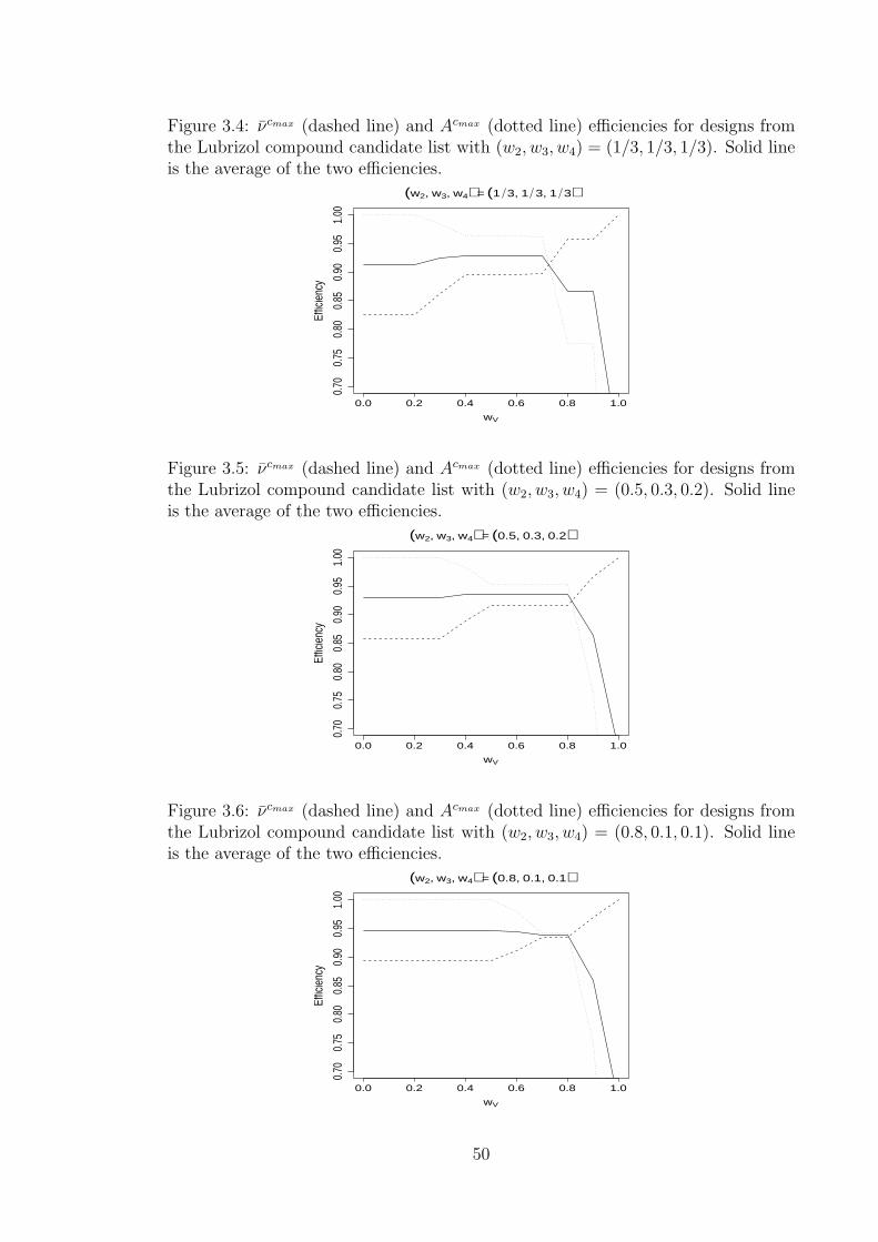
Figure 3.4: νcmax (dashed line) and Acmax (dotted line) efficiencies for designs fromthe Lubrizol compound candidate list with (w2, w3, w4) = (1/3, 1/3, 1/3). Solid lineis the average of the two efficiencies.

0.0 0.2 0.4 0.6 0.8 1.0

0.70

0.75

0.80

0.85

0.90

0.95

1.00

(w2, w3, w4) = (1 3, 1 3, 1 3)

wV

Effic

ienc

y

Figure 3.5: νcmax (dashed line) and Acmax (dotted line) efficiencies for designs fromthe Lubrizol compound candidate list with (w2, w3, w4) = (0.5, 0.3, 0.2). Solid lineis the average of the two efficiencies.

0.0 0.2 0.4 0.6 0.8 1.0

0.70

0.75

0.80

0.85

0.90

0.95

1.00

(w2, w3, w4) = (0.5, 0.3, 0.2)

wV

Effic

ienc

y


0.0 0.2 0.4 0.6 0.8 1.0

0.70

0.75

0.80

0.85

0.90

0.95

1.00

(w2, w3, w4) = (0.8, 0.1, 0.1)

wV

Effic

ienc

y

50


0.0 0.2 0.4 0.6 0.8 1.0

0.70

0.75

0.80

0.85

0.90

0.95

1.00

(w2, w3, w4) = (0.1, 0.1, 0.8)

wV

Effic

ienc

y

Table 3.14: Comparison of designs for the Lubrizol compound candidate list for(w2, w3, w4) = (1/3, 1/3, 1/3) and wV = 0, 0.1, . . . , 0.7, 0.8

wV ν(2) ν(3) ν(4) A∗(2)/A(2) A∗(3)/A(3) A∗(4)/A(4)0 1.14 1.37 1.78 0.29 0.23 0.170.1 1.14 1.37 1.78 0.29 0.23 0.170.2 1.14 1.37 1.78 0.29 0.23 0.170.3 1.13 1.32 1.66 0.28 0.22 0.170.4 1.12 1.29 1.55 0.27 0.22 0.170.5 1.12 1.29 1.55 0.27 0.22 0.170.6 1.12 1.29 1.55 0.27 0.22 0.170.7 1.11 1.28 1.56 0.27 0.22 0.170.8 1.09 1.21 1.40 0.21 0.18 0.14

Table 3.15: Comparison of designs for the Lubrizol compound candidate list for(w2, w3, w4) = (0.5, 0.3, 0.2) and wV = 0, 0.1, . . . , 0.7, 0.8

wV ν(2) ν(3) ν(4) A∗(2)/A(2) A∗(3)/A(3) A∗(4)/A(4)0 1.14 1.37 1.78 0.29 0.23 0.170.1 1.14 1.37 1.78 0.29 0.23 0.170.2 1.14 1.37 1.78 0.29 0.23 0.170.3 1.14 1.37 1.78 0.29 0.23 0.170.4 1.13 1.32 1.66 0.28 0.22 0.170.5 1.11 1.28 1.56 0.27 0.22 0.170.6 1.11 1.28 1.56 0.27 0.22 0.170.7 1.11 1.28 1.56 0.27 0.22 0.170.8 1.11 1.28 1.56 0.27 0.22 0.17

51

3.6 Discussion

We have shown that variance inflation factors can be a useful tool when considering

supersaturated designs. They can easily be used to assess existing competing designs

and can also give an indication of which factors should be assigned to which columns

when some prior information is available. VIFs can also be incorporated into widely

applicable criteria used to generate designs where the factors are at two or more

levels, or where their levels cannot be set independently.

In the two-level case, we show that our new designs perform favourably in many

cases compared with existing alternatives. By using Criterion 4 and allowing some

imbalance in the designs, we can often achieve good VIFs and E(s2) values.

A considerable advantage of considering VIFs is that we are not restricted to look-

ing only at dependencies between pairs of factors (as we are with E(s2)). This

is particularly beneficial when considering mid-size experiments, where there could

reasonably be three or four active factors.

We have shown that the weight, wV , on ν(c) in compound Criterion 4 can be adjusted

to the requirements of a particular experiment, in order to achieve more balance, a

broader spread of the factors, or less linear dependency between the columns. This

makes our criterion more flexible than some existing approaches.

Unless strong prior information that some factors are active is available, we recom-

mend setting (w2, w3, . . . , wcmax) = (1/(cmax − 1), 1/(cmax − 1), . . . , 1/(cmax − 1)) as

such a design will give more uniform performance across different numbers of true

active factors.

The sacrifice required in order to achieve the advantages of the variance inflation

factor based criteria is the computational time required to find the designs. Because

so many models are being considered, computational restrictions may prohibit the

generation of large designs, particularly if we wish to incorporate five or more active

factors into the criterion. However, as computer time is generally cheap compared

to experimentation, the advantages of the new designs could make this investment

of time worthwhile.

52

Chapter 4

Supersaturated experiments forscreening interaction effects withapplication to robust productdesign

Interactions between control and noise factors are often utilised in robust product

design. Experiments can be designed to find settings of the control factors that

dampen the variability in the response due to variability in the noise factors by

exploiting control by noise interactions. One problem with such experiments is

that, even for a moderate number of control and noise factors, a large number of

interactions will be of interest. Traditional methods of planning experiments result

in plans with many runs, which can be costly. In such a situation, an alternative is

a supersaturated experiment, in which the number of observations is less than the

number of factorial effects requiring estimation.

A new criterion for constructing supersaturated designs with both control and noise

factors is described. By allowing complete aliasing between effects that are not of

interest, the criterion results in designs with only minimal partial aliasing between

effects of interest. A flexible algorithmic approach is used to find designs for any

number of control and noise factors, and also any run size. The performance of the

new designs in relation to competing methods is discussed and some examples are

presented to illustrate, in particular, how the new designs have a higher power to

detect those effects of interest that have a substantive impact on the response.

53

4.1 Introduction

In industrial experimentation a key tool for improving quality of products and pro-

cesses is the exploitation of interactions between so called control factors (denoted

C) and noise factors (denoted N). Control factors can be set in the product specifi-

cation, whereas noise factors cannot. However, it is often possible to mimic the noise

factors in an experiment, and hence provide useful information on control by noise

(C×N) interactions. Many such experiments have been discussed in the literature,

for example Miller et al. (1993) described an experiment in automobile manufactur-

ing. An experiment with five control and three noise factors was conducted to try to

find settings of the control factors which resulted in minimal distortion of the drive

pinion and gear set under heat treatment. Vine et al. (2008) described an experiment

to identify important factors affecting the cold start performance of a new genera-

tion engine at Jaguar cars. Reducing performance variability was important and as

such, both control and noise factors were involved. A group screening approach was

pursued, whereby factors under investigation are partitioned into groups. In each

run, all factors within a group are set to the same level and hence factors within the

same group are completely confounded with each other.

Robust design was first discussed by Taguchi (1986) who proposed crossing two de-

sign matrices (arrays); one for control factors and one for noise factors. However,

this approach was criticised because the number of runs required was often pro-

hibitively large. Welch et al. (1990) proposed using a combined array, incorporating

both control and noise factors. This idea was then further explored by Shoemaker

et al. (1991), who illustrated how a combined array can result in smaller experi-

ments. More recently, Wu and Zhu (2003) and Zhu et al. (2007) have proposed

aberration-type criteria to choose the best combined array. One of the drawbacks is

that many of these designs have effects of interest which are completely aliased with

other effects. Loeppky et al. (2006) also proposed an aberration-type criterion for

non-regular designs. These have main effects and two-factor interactions which are

partially aliased. Kang and Joseph (2009) proposed a Bayesian criterion for select-

ing the optimal combined array. This criterion incorporated the concept of effect

hierarchy in addition to reflecting the differing importance of certain effects. The

54

criterion focussed on efficient estimation of the variance and as such places much

emphasis on noise main effects and control by noise interactions. However, the au-

thors acknowledge that the criterion could be altered to allow better estimation of

the mean of the process. The designs could have any number of runs and may also

be non-regular. Lewis and Dean (2001) instead used two-stage group screening to

provide information on important interactions.

Supersaturated experiments traditionally have more factors to be investigated than

runs. However, this definition can be extended to the case where there are more

parameters of interest than runs. They are particularly beneficial when there are a

large number of parameters to investigate, but experimentation is very expensive.

The idea was first introduced by Box (1959) in the discussion of Satterthwaite (1959),

who suggested they be designed using random balance. Booth and Cox (1962)

provided the first systematic way of constructing supersaturated designs (SSDs)

when they proposed the E(s2) criterion. After many years with minimal interest

in SSDs, Lin (1993) and Wu (1993) revived the topic with a construction method

based on Hadamard matrices. More recent work on criteria for SSDs includes that

of Jones et al. (2008) who proposed Bayesian D-optimality.

There has been very little work on using supersaturated designs to screen for in-

teractions. Wu (1993) supplemented an SSD with interaction columns and stated

that they could be used to study either the interaction or another factor. Liu et al.

(2007) added interaction columns to k-circulant SSDs. However, they couldn’t mea-

sure all interactions since some of the columns would be identical to each other. Lin

(1998) suggested analysing main effects plans as a supersaturated design by also

considering two-factor interactions.

In the vast majority of combined array and cross array experiments, some effects

potentially of interest are completely confounded. This chapter illustrates how su-

persaturated experiments can be designed so that none of the effects of interest are

completely confounded with each other, in addition to exploiting the potential for

cost savings due to reduced experiment sizes. The new approach is very flexible and

can deal with any number of runs and factors.

This chapter is organised as follows. Section 4.2 defines a new criterion for two-level

55

supersaturated experiments which is more appropriate than existing criteria when

we consider the robust parameter design setting. Section 4.3 presents some examples

to illustrate the benefits of the new criterion. Some further discussion is presented

in Section 4.4. Tables of some new designs we generate are available on the attached

CD.

4.2 Choosing supersaturated designs with control

and noise factors

4.2.1 Criteria

Throughout the chapter we consider the model

Y = Xβ + ε , (4.1)

where Y is the n× 1 response vector, X is an n× p model matrix, β is a vector of p

unknown coefficients and ε is a vector of independent normally distributed random

errors with mean 0 and variance σ2.

Supersaturated experiments have a necessarily complex partial aliasing structure.

This results in correlated estimators of the factorial effects and can make inferring

causation difficult. Thus many design construction criteria focus on trying to min-

imise the level of partial aliasing in a design (i.e. construct the design so that the

columns of the model matrix are as near orthogonal as possible).

Suppose we were to consider only main effects in an experiment of n runs and m

factors. Then X is an n × (m + 1) model matrix. We assume that each of the m

factors has two levels, coded ±1. The first column of X is 1n = [1, . . . , 1]T , with

column k corresponding to the levels of the (k − 1)th factor (k = 2, . . . ,m + 1).

Booth and Cox (1962) proposed a criterion for two-level SSDs for m main effects

that selects a design by minimising the sum of the squared inner-products between

columns k and l of X (k, l = 2, . . . ,m+ 1). We extend this definition to unbalanced

designs and include the inner-product of the first column with every other column

of X to give the objective function

56

E(s2) =2

m(m+ 1)

∑k<l

s2kl ,

where skl is the klth element of XTX (k, l = 1, . . . ,m + 1). Each s2kl gives an

indication of the level of partial aliasing between columns k and l, with larger values

meaning stronger aliasing. This can easily be extended to the case where we wish

to screen all two-factor interactions. In this case, X is an n× p model matrix with

p = 1 + m + m(m − 1)/2. Columns m + 2, . . . , p of X contain the levels of the

two-factor interactions between factors k − 1 and l − 1 (k, l = 2, . . . ,m + 1 and

k < l). We have

E(s2) =2

p(p− 1)

∑i<j

s2ij , (4.2)

where i, j = 1, . . . , p.

However, in the control by noise setting it is not particularly beneficial to estimate

noise (N) main effects or noise by noise (N × N) interactions. This is because we

have no control over their values in the real life process under investigation. All

we are concerned about in the experiment is that they are not strongly aliased

with terms that we are interested in, particularly control (C) main effects, C × C

interactions and C × N interactions. Low levels of partial aliasing means that

attributing observed effects to the truly active factors in the analysis is more likely.

We propose a new objective function to reflect the importance of certain effects,

modifying (4.2) so that it does not take into account aliasing amongst effects which

are not of interest. In general we assume there is a set S1 that contains the column

numbers in X corresponding to the effects of interest and a set S2 which contains

the column numbers corresponding to the effects which are not of interest. In a

similar vein, Srivastava (1975) found search designs by also partitioning effects into

different sets; one which the experimenter definitely wanted to estimate, one which

he definitely did not, and another which may contain a relatively small number of

active effects. He pointed out that the experimenter, in addition to estimating all

the effects in the first set, may wish to search the final set and pick out non-negligible

effects. DuMouchel and Jones (1994) partitioned effects into two groups, with those

57

thought likely to be active (primary) in one group and the remainder (potential) in

the other.

Since those effects in S2 are not of any interest, we ignore inner products between

their columns in a modified objective function in order to get overall more favourable

aliasing amongst the terms which are of interest. We call this effect-focussed E(s2):

ES1(s2) =

2

k

( ∑i,j=1,...,p; i<j

s2ij −

∑i,j∈S2; i<j

s2ij

),

where k = p(p − 1) − v(v − 1) is the number of inner products corresponding to

parameters of interest and v denotes the size of S2.

In the special case of the control by noise setting, we do not take into account inner

products amongst noise main effects, N × N interactions and also between noise

main effects and N ×N interactions. Then we get overall more favourable aliasing

amongst the terms of interest. Since, when using a supersaturated design, there are

not enough runs available to estimate all effects simultaneously, we will essentially

consider submodels in the analysis. Hence low levels of aliasing will also result in

low bias. Jones and Nachtsheim (2009) proposed a two-part criterion, minimising

the sum of the squared elements of the alias matrix, subject to a constraint on the

D-efficiency of the design. In the examples they consider, there were always enough

runs to be able to estimate all effects of interest, which will not be the case in this

chapter.

We assume a particular ordering of the terms in the model matrix X. Let pC and

pN be the number of control and noise main effects. Further, let pCC = pC(pC−1)/2

and pNN = pN(pN −1)/2 be the number of C×C and N×N interactions. Columns

2, . . . , pC +1 of X represent control main effects and columns pC +2, . . . , pC +pN +2

represent noise main effects. The following pCC columns represent C×C interactions

and the next pCpN represent C×N interactions. Finally, columns p−pNN +1, . . . , p

represent N×N interactions. For ease of notation we define SN = {pC +2, . . . , pC +

pN + 1} and SNN = {p − pNN + 1, . . . , p}. Then S2 = {SN ,SNN} and the effect-

focussed E(s2) objective function is as follows;

58

ES1(s2) =

2

k

( ∑i,j=1,...,p; i<j

s2ij −

∑i,j∈SN ; i<j

s2ij −

∑i∈SNN ; j∈SN

s2ij −

∑i,j∈SNN ; i<j

s2ij

), (4.3)

where k = p(p− 1)− pN(pN − 1)− pNN(pNN − 1)− 2pNNpN . Notice that the second

term of (4.3) excludes all the sij corresponding to inner products amongst noise main

effects. The third term excludes all sij corresponding to inner products between

noise main effects and N ×N interactions, since we do not mind if the estimators of

these effects are correlated. The fourth term excludes all sij corresponding to inner

products amongst N ×N interaction columns.

Although Marley and Woods (2010) showed that unbalanced supersaturated designs

can achieve high power to identify active effects, it is not desirable that the designs

be extremely unbalanced. Therefore it can be beneficial to give slightly more weight,

w ≥ 1, in the objective function to inner products of effects with the intercept. This

can help to achieve an acceptable degree of balance in the designs, without restricting

to only balanced designs. The resulting effect-focussed E(s2) criterion is

minimise ES1(s2(w)) =

2

k

(w∑

i=2,...,p

s2i1 +

∑i,j=2,...,p; i<j

s2ij−

∑i,j∈SN ; i<j

s2ij −

∑i∈SNN ; j∈SN

s2ij −

∑i,j∈SNN ; i<j

s2ij

). (4.4)

The first term in 4.4 gives more weight to inner products involving the intercept term.

Advice on choosing w is given in Section 4.3.4. When w = 1, (4.4) is equivalent

to minimising the objective function in (4.3). Similarly, the same benefits can be

achieved by modifying (4.2) to give the intercept-weighted E(s2) criterion:

minimise E(s2(w)) =2

p(p− 1)

(w∑

i=2,...,p

s2i1 +

∑i,j=2,...,p; i<j

s2ij

). (4.5)

We note that when |S2| = 0, 1 (4.4) and (4.5) are equivalent. When generating

designs using (4.4) and (4.5) it is recommended that the maximum absolute cor-

relation between a pair of distinct columns of interest is constrained to be below

59

a certain value. This will make inferring the causation of the effects easier, hence

reducing the chance of type I and type II errors in the analysis. Based on previous

experience we recommend that this value be 0.6. A coordinate exchange algorithm

(Meyer and Nachtsheim, 1995) incorporating this constraint can be used to generate

designs using (4.4) and (4.5). All designs generated in this chapter use 4,000 random

starts of the algorithm. It is worth noting that if we wish to generate completely

balanced designs, a columnwise algorithm (Li and Wu, 1997) could be used.

Some new designs in this chapter are also compared with those generated using the

Bayesian D-optimality criterion of Jones et al. (2008). Under a Bayesian paradigm

with conjugate prior distributions for β and σ2 (O’Hagan and Forster, 2004), the

posterior variance-covariance matrix for β is proportional to (XT X+K/τ 2)−1. Here,

τ 2K−1 is proportional to the prior variance-covariance matrix for β. The resulting

criterion is

maximise DBayes = |XTX + K/τ 2|1/p ,

where τ 2 is a tuning parameter reflecting the available prior information. This prior

information can be viewed as equivalent to having sufficient additional runs to allow

estimation of all effects. Jones et al. (2008) regarded the intercept as a primary

term with large prior variance, and all others as potential terms with small prior

variances, see DuMouchel and Jones (1994), and set

K = K1 =

(0 01×(p−1)

0(p−1)×1 I(p−1)×(p−1)

).

In order to prioritise the estimation of certain terms over others, we can alter the

diagonal values in the matrix K. We give a larger prior variance to terms which

are of interest by using a low value in the corresponding position in the K matrix.

Let the ith diagonal element of K be denoted by ki. For K1, k1 = 0 and ki = 1,

i = 2, . . . , p. Here, all terms except the intercept have equal prior variance. Suppose

instead we set k1 = 0, ki = 0.1 for i corresponding to all terms which are of interest

(i.e. those in S1) and ki = 1 for all terms not of interest. Call this matrix K2.

Then when using Bayesian D-optimality with K2, we are strongly prioritising the

60

estimation of effects which are of interest over those which are not.

4.3 Examples

Three detailed examples are presented to illustrate the benefits of using a SSD

generated using effect-focussed E(s2). They demonstrate advantages both over other

supersaturated approaches and also the more traditional methods for robust product

design experiments such as combined arrays. We then briefly consider a much wider

range of experiments and describe when our new criterion is most effective. In all

examples we assume model (4.1).

4.3.1 Example 1: 6 control and 4 noise factors

Suppose we have six control and four noise factors. A traditional approach might

use a 64-run resolution IV 210−4 combined array. Russell et al. (2004) proposed

a set of generating words for such an experiment. This was chosen so that the

resulting design sequentially had as many clear control main effects, control by noise

interactions and control by control interactions as possible. A clear effect is one

which is completely free from aliasing with all other effects. However, the proposed

scheme results in all control by control interactions being completely aliased with

at least one other control by control interaction. Further, the array uses many more

runs than is desirable for screening purposes. We demonstrate how costs can be

reduced, and complete aliasing of effects of interest can be eliminated, with little

impact on the correct identification of active factors. Suppose instead that we use

a SSD with 28 runs, where the model matrix incorporates the intercept, all main

effects and all 2-factor interactions. We generated designs using effect-focussed E(s2)

and intercept-weighted E(s2) with w = 1, 2, 4, 6. Setting w = 6 produced designs

which are only slightly unbalanced. For comparison, we also generated a Bayesian

D-optimal design with K1 for 10 factors and all two-factor interactions, arbitrarily

labelling the first 6 columns as control factors. Finally, a Bayesian D-optimal design

with K2 was generated. Some of the properties of the four designs are given in Table

4.1.

61

Table 4.1: Properties of 28-run designs for 6 control and 4 noise factors generatedusing effect-focussed (E-F) E(s2)-, intercept-weighted (I-W) E(s2)- and Bayesian D(B-D) -optimality. Maximum absolute correlation between any pair of columns (ofinterest) denoted by rmax (r∗max). Number of columns with absolute value of thecolumn sum equal to q defined by φq.

Design E-F (w = 6) I-W (w = 6) B-D (K = K1) B-D (K = K2)ES1(s

2(1)) 16.49 17.70 17.63 18.14E(s2(1)) 17.60 17.28 17.27 18.33DBayes(K1) 7.30 7.33 7.33 7.26DBayes(K2) 3.08 3.11 3.10 3.17rmax 1.00 0.50 0.58 0.58r∗max 0.50 0.50 0.58 0.58φ2 24 30 28 26φ4 2 1 5 4φ6 0 0 0 2

Notice that all four designs perform similarly well under DBayes with both K1 and

K2. The Bayesian D-optimal design with K1 and the intercept-weighted E(s2)-

optimal design perform similarly well under E(s2(1)) but similarly poorly under

ES1(s2(1)), where our new design displays a clear advantage (16.49 compared to

17.70 and 17.63). The Bayesian D-optimal design with K2 is poor when evaluated

under ES1(s2(1)) and E(s2(1)). We denote the maximum absolute correlation be-

tween any pair of columns in the model matrix by rmax. Similarly, r∗max denotes

the maximum absolute correlation between any pair of columns of interest (that is,

we excluding pairwise correlations amongst noise factor columns, amongst N × N

columns and between noise factor and N × N columns). Notice that rmax = 1

for the effect-focussed E(s2)-optimal design. This means that some parameters are

completely aliased. However, there is no complete aliasing between any parameters

which are of interest since r∗max < 1.

We define φq as the number of columns of the model matrix with absolute value of the

column sum equal to q. This can be used to indicate the degree of imbalance present

in the design. We see from Table 4.1 that all four designs are slightly unbalanced,

with a maximum absolute column sum of 4 for three out of the four designs, and 6

for the Bayesian D-optimal design with K2.

We point out that the intercept-weighted E(s2)-optimal design may not be E(s2)-

62

Table 4.2: Number of active effects in each of 10 scenarios for the simulation studyfor Example 1

Scenario Main effects C × C C ×N N ×N1 3 0 0 02 2 1 2 03 3 1 1 14 4 1 3 15 4 2 2 06 4 3 1 07 5 2 2 08 5 2 2 19 5 2 3 110 6 2 3 2

optimal due to the extra weight placed on inner products with columns involving

the intercept.

To investigate the performance of the four SSDs, a simulation study was performed.

This consisted of investigating 10 different scenarios of varying difficulty. Table 4.2

shows the number of active effects from each category that were present in each

scenario. The scenarios range from having only a small number of active main

effects, to having several active main effects along with various interactions.

Each scenario was run 1000 times with the active factors chosen at random from the

relevant categories. All active factors were simulated from the distribution N(4, 0.2)

and all inactive factors were simulated from N(0, 0.2). Data were generated from

model (4.1) with error, ε from N(0, 1). Note that the scenarios did not necessarily

obey effect heredity.

The data were analysed using the Gauss-Dantzig selector (GDS), which was shown

by Marley and Woods (2010) to be a promising analysis method for SSDs. The GDS

belongs to a class of continuous variable selection techniques known as shrinkage

methods, where each coefficient is shrunk towards zero at a different rate. The GDS

is an extension of the original Dantzig selector method proposed by Candes and Tao

(2007), where the estimator β is the solution to

63


Here ||β||1 = |β0|+ . . .+ |βm| is the l1 norm, ||β||∞ = max(|β0|, . . . , |βm|) is the l∞

norm, and δ is a tuning constant.

The GDS is a two-stage approach developed by Candes and Tao (2007). This was

first used for the analysis of supersaturated designs by Phoa et al. (2009). Initially

the Dantzig selector is used to identify the active factors, and those factors whose

coefficient estimates are greater than γ are retained. Second, least squares estimates

are found by regressing the response on the set of retained factors. The tuning

constant γ represents the size of the smallest coefficient that would result in a factor

being considered active and, in practice, could be elicited from subject experts.

To implement the GDS, we reformulate (4.6) as a linear program and solve using

the package lpSolve (Berkelaar, 2007) in R (R Development Core Team, 2009). An

automated selection procedure with BIC is used to choose the tuning constant δ and

we set γ = 1.5. For more details see Marley and Woods (2010), Candes and Tao

(2007) and Phoa et al. (2009).

We compare the designs using two summary measures;

1. Power; the average proportion of active factors correctly identified. This is a

larger-the-better measure.

2. Type I error rate; the average proportion of inactive factors which are declared

active. This is a smaller-the-better measure.

Since we are only interested in certain effects, power is divided into power for C, N ,

C × C, C ×N and N ×N effects. Type I error rate is considered only for C main

effects, C × C and C ×N interactions combined.

Power for different effects and Type I error rate for the effect-focussed E(s2)-optimal

design is given in Table 4.3. The corresponding figures for the intercept-weighted

E(s2)-optimal design are shown in Table 4.4, and for the Bayesian D-optimal designs

with K1 and K2 in Tables 4.5 and 4.6. An NA in a table means that a particular

effect was not present in the given scenario.

64

Table 4.3: Powers for various effects and Type I error rate for the 28-run design forExample 1 generated using effect-focussed E(s2) with w = 6

Scenario Power Type I error rateC N C × C C ×N N ×N

1 1.00 0.97 NA NA NA 0.012 0.99 0.92 0.98 0.99 NA 0.023 0.98 0.89 0.95 0.98 0.50 0.024 0.93 0.86 0.83 0.89 0.45 0.055 0.94 0.90 0.89 0.93 NA 0.046 0.93 0.89 0.87 0.92 NA 0.047 0.92 0.87 0.84 0.88 NA 0.058 0.88 0.82 0.79 0.86 0.42 0.069 0.84 0.80 0.74 0.80 0.39 0.0710 0.79 0.73 0.68 0.75 0.36 0.10

Table 4.4: Powers for various effects and Type I error rate for the 28-run design forExample 1 generated using intercept-weighted E(s2) with w = 6


1 1.00 1.00 NA NA NA 0.012 0.97 0.98 0.97 0.97 NA 0.023 0.95 0.94 0.91 0.96 0.94 0.034 0.85 0.86 0.81 0.84 0.83 0.065 0.90 0.91 0.86 0.88 NA 0.046 0.89 0.91 0.86 0.88 NA 0.057 0.85 0.88 0.82 0.83 NA 0.068 0.82 0.83 0.77 0.80 0.78 0.079 0.74 0.76 0.69 0.73 0.74 0.0910 0.67 0.67 0.58 0.66 0.65 0.12

65

Table 4.5: Powers for various effects and Type I error rate for the 28-run design forExample 1 generated using Bayesian D-optimality with K = K1


1 1.00 0.99 NA NA NA 0.012 0.96 0.97 0.98 0.97 NA 0.023 0.94 0.96 0.94 0.95 0.96 0.034 0.81 0.85 0.82 0.83 0.83 0.065 0.89 0.87 0.86 0.89 NA 0.056 0.89 0.85 0.86 0.88 NA 0.057 0.84 0.85 0.80 0.82 NA 0.068 0.78 0.79 0.77 0.79 0.79 0.089 0.74 0.74 0.72 0.75 0.73 0.0910 0.65 0.65 0.59 0.67 0.66 0.13

Table 4.6: Powers for various effects and Type I error rate for the 28-run design forExample 1 generated using Bayesian D-optimality with K = K2


1 1.00 0.99 NA NA NA 0.012 0.97 0.92 0.97 0.97 NA 0.023 0.94 0.90 0.93 0.94 0.88 0.034 0.86 0.75 0.87 0.84 0.70 0.065 0.91 0.80 0.89 0.89 NA 0.046 0.91 0.82 0.86 0.90 NA 0.047 0.87 0.76 0.83 0.84 NA 0.068 0.83 0.71 0.80 0.80 0.66 0.089 0.76 0.62 0.75 0.73 0.59 0.0910 0.68 0.54 0.69 0.66 0.48 0.12

66

Notice from Tables 4.3-4.6 that the effect-focussed E(s2)-optimal design always beats

the intercept-weighted E(s2)- and Bayesian D-optimal (with K1) designs under

power for C main effects, C × C and C × N interactions which indicates the clear

benefits of our new criterion over existing criteria for SSDs. We also see comparable

or even more favourable Type I error rates for our new design. Notice that power for

N × N interactions is particularly low for the effect-focussed E(s2)-optimal design

due to some of these effects being completely aliased with each other. However,

since we cannot control these effects in practice, we accept the trade off of better

identifiability of C main effects, C ×C and C ×N interactions. The effect-focussed

E(s2)-optimal design also outperforms the BayesianD-optimal design with K2 under

power for C main effects and C × N interactions and Type I error rate, whilst

performing similarly under power for C × C interactions.

Notice that as we increase the number of active effects, the powers tend to decrease

and Type I error rates increase. This is in line with an observation of Marley and

Woods (2010). However, for the effect-focussed E(s2)-optimal design, the power is

still very high, even for scenario 8, which has a relatively large number of active

main effects (five) and interactions (five). This is achieved using only 28 runs - con-

siderably less than the 64 runs that may have been used in the traditional combined

array approach, and without the complete aliasing of effects of interest.


Now consider an experiment with 4 control and 6 noise factors. In this case, we would

expect to see considerable benefits from using effect-focussed E(s2)-optimality, since

we have more noise factors than control factors. Therefore, we are able to sacri-

fice good aliasing between many effects in order to achieve more desirable alias-

ing between effects of interest. As in Example 1, we generate SSDs using effect-

focussed E(s2) and intercept-weighted E(s2) with w = 1, 2, 4, 6 and also Bayesian

D-optimality with K1 and K2. The designs all have 24 runs. In this instance, set-

ting w = 4 produced designs which achieved a reasonable degree of balance. Some

of the properties of the four designs are given in Table 4.7.

Notice that the effect-focussed E(s2)-optimal design has a much lower value of

67



2(1)) 10.43 16.15 16.49 16.43E(s2(1)) 18.83 16.02 16.02 19.11DBayes(K1) 5.39 5.53 5.53 5.39DBayes(K2) 2.83 2.79 2.86 2.95rmax 1.00 0.58 0.58 1.00r∗max 0.44 0.58 0.58 0.58φ2 22 28 27 18φ4 8 2 0 8φ6 6 0 1 0φ8 0 0 0 4

ES1(s2(1)) than the other three designs. It also has a lower value of r∗max and again

displays complete aliasing between some effects which are not of interest. For this

example, the Bayesian D-optimal design with K2 also displays complete aliasing,

and also has the most unbalanced columns of all the designs (φ8 = 4).

As in Section 4.3.1, the four designs were compared by way of a simulation study.

Similar scenarios to those in Section 4.3.1 were used, and are detailed in Table 4.8.

Each scenario was run and analysed in the same way as 4.3.1.

Power for different effects and Type I error rate for the effect-focussed E(s2)-optimal

design is given in Table 4.9. The corresponding figures for the intercept-weighted

E(s2)-optimal design are shown in Table 4.10, and for the Bayesian D-optimal de-

signs with K1 and K2 in Tables 4.11 and 4.12.

Notice that we see large improvements in power for C main effects, C×C interactions

and C × N interactions for the effect-focussed E(s2)-optimal design. For example,

for scenario 5, where there are 4 active main effects and 4 active interactions, the

powers for C main effects, and C×N interactions are 0.95 and 0.94. This compares

to only 0.78 and 0.72 for the intercept-weighted E(s2)-optimal design. Similarly, the

Type I error rate for this scenario is only 0.03 for the effect-focussed E(s2)-optimal

design compared to 0.07 for the intercept-weighted E(s2)-optimal design. It is also

68


Scenario Main effects C × C C ×N N ×N1 3 0 0 02 2 0 2 13 3 1 1 14 4 1 3 15 4 0 2 26 4 0 1 37 5 0 2 28 5 1 2 29 5 1 3 210 6 2 3 2

Table 4.9: Powers for various effects and Type I error rate for the 24-run design forExample 2 generated using effect-focussed E(s2) with w = 4


1 1.00 0.64 NA NA NA 0.012 0.97 0.60 NA 0.97 0.21 0.023 0.98 0.57 0.94 0.97 0.19 0.024 0.88 0.56 0.81 0.87 0.17 0.065 0.95 0.53 NA 0.94 0.17 0.036 0.97 0.51 NA 0.95 0.16 0.037 0.94 0.52 NA 0.92 0.17 0.048 0.90 0.52 0.79 0.85 0.16 0.069 0.85 0.50 0.73 0.80 0.16 0.0810 0.76 0.48 0.66 0.70 0.14 0.11

69

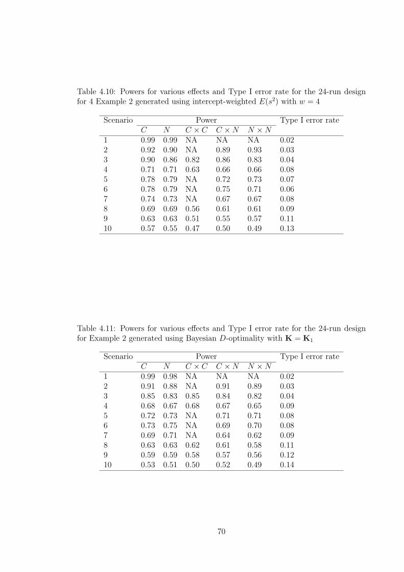
Table 4.10: Powers for various effects and Type I error rate for the 24-run designfor 4 Example 2 generated using intercept-weighted E(s2) with w = 4


1 0.99 0.99 NA NA NA 0.022 0.92 0.90 NA 0.89 0.93 0.033 0.90 0.86 0.82 0.86 0.83 0.044 0.71 0.71 0.63 0.66 0.66 0.085 0.78 0.79 NA 0.72 0.73 0.076 0.78 0.79 NA 0.75 0.71 0.067 0.74 0.73 NA 0.67 0.67 0.088 0.69 0.69 0.56 0.61 0.61 0.099 0.63 0.63 0.51 0.55 0.57 0.1110 0.57 0.55 0.47 0.50 0.49 0.13

Table 4.11: Powers for various effects and Type I error rate for the 24-run designfor Example 2 generated using Bayesian D-optimality with K = K1


1 0.99 0.98 NA NA NA 0.022 0.91 0.88 NA 0.91 0.89 0.033 0.85 0.83 0.85 0.84 0.82 0.044 0.68 0.67 0.68 0.67 0.65 0.095 0.72 0.73 NA 0.71 0.71 0.086 0.73 0.75 NA 0.69 0.70 0.087 0.69 0.71 NA 0.64 0.62 0.098 0.63 0.63 0.62 0.61 0.58 0.119 0.59 0.59 0.58 0.57 0.56 0.1210 0.53 0.51 0.50 0.52 0.49 0.14

70



1 0.98 0.63 NA NA NA 0.022 0.92 0.55 NA 0.92 0.52 0.033 0.93 0.54 0.98 0.87 0.49 0.044 0.82 0.42 0.88 0.76 0.34 0.095 0.84 0.47 NA 0.79 0.41 0.076 0.80 0.48 NA 0.79 0.40 0.077 0.78 0.44 NA 0.75 0.35 0.098 0.76 0.43 0.88 0.72 0.37 0.109 0.75 0.40 0.85 0.69 0.31 0.1210 0.69 0.35 0.78 0.60 0.27 0.15

worth noting the consistently high powers, especially for scenarios 1-8, despite the

fact that we are using a design with only 24 runs.

Using K2 instead of K1 in the Bayesian D-optimality criterion results in a design

with higher power for effects of interest. However, neither design beats the perfor-

mance of the effect-focussed E(s2)-optimal design.


In this section we present an example with 5 control and 3 noise factors. Miller

et al. (1993) considered an experiment with the same number of factors where two

replicates of a 128-run cross array were used. Here, we apply our new methods to

construct experiments with only 20 runs, and demonstrate how they may perform

in practice. This example also illustrates that higher power for effects of interest can

still be achieved by using effect-focussed E(s2)-optimality, despite there only being

a relatively small number of noise factors and noise by noise interactions. The same

procedure as for Examples 1 and 2 was followed, with four SSDs being generated.

Some of the properties of the four designs are given in Table 4.13.

In this case, the effect-focussed E(s2)-, intercept-weighted E(s2)- and Bayesian D-

optimal (K1) designs perform similarly under E(s2(1)) and DBayes(K1). However,

the intercept weighted E(s2)- and Bayesian D-optimal designs do considerably worse

71



2(1)) 10.49 12.39 12.39 12.71E(s2(1)) 12.18 12.18 12.16 12.72DBayes(K1) 6.86 6.86 6.87 6.81DBayes(K2) 3.01 3.06 3.07 3.15rmax 1.00 0.41 0.50 0.50r∗max 0.41 0.41 0.50 0.50φ2 0 0 8 13φ4 4 3 1 1φ6 0 0 0 1φ8 0 0 0 1


Scenario Main effects C × C C ×N N ×N1 3 0 0 02 2 2 0 03 2 0 1 04 2 2 1 05 2 0 0 26 2 0 1 17 3 1 1 18 4 1 2 2

than the effect-focussed E(s2) design when evaluated under ES1(s2(1)). All designs

have reasonably low r∗max. Again, the Bayesian D-optimal design with K2 is the most

unbalanced. This time eight different simulation scenarios are considered (shown in

Table 4.14).

The simulation was performed as in Sections 4.3.1 and 4.3.2. Power for different

effects and Type I error rate for the design generated using effect-focussed E(s2)

is given in Table 4.15. The corresponding figures for the designs generated using

intercept-weighted E(s2) and Bayesian D-optimality are shown in Tables 4.16, 4.17

and 4.18.

72

Table 4.15: Powers for various effects and Type I error rate for the 20-run designfor Example 3 generated using effect-focussed E(s2) with w = 4


1 1.00 0.95 NA NA NA 0.022 0.98 0.93 0.98 NA NA 0.033 0.99 0.93 NA 1.00 NA 0.024 0.95 0.90 0.96 0.95 NA 0.045 1.00 0.64 NA NA 0.03 0.026 0.99 0.79 NA 0.99 0.04 0.027 0.96 0.80 0.94 0.95 0.04 0.048 0.87 0.63 0.85 0.84 0.04 0.08

Table 4.16: Powers for various effects and Type I error rate for the 20-run designfor Example 3 generated using intercept-weighted E(s2) with w = 4






73




It can be seen that for scenarios 1-4, the four designs perform similarly, with very

high powers for C main effects, C × C interactions and C × N interactions and

similar Type I error rates. However, for scenarios 5-8 the effect-focussed E(s2)-

optimal design has higher power for C main effects, C × C interactions and C ×N

interactions and also a lower Type I error rate. Thus using our new criterion can be

beneficial even when there are only a small number of noise factors. The powers for

scenarios 1-7 are all very high, indicating how successful a supersaturated design can

be. This design also has the benefit of having 12 fewer runs than a more traditional

32 run combined array, thus dramatically reducing experimental cost.

4.3.4 Other examples

Examples 1, 2 and 3 illustrate how the new effect-focussed E(s2)-optimality criterion

can produce designs which perform better in practice than other supersaturated

approaches. They also demonstrate how high power and low Type I error rate for

effects of interest can be achieved in only a small number of runs. Many other

examples for pC and pN ranging from 3 to 6 and varying run sizes were investigated

and trends following those seen in Examples 1, 2 and 3 were observed. The largest

gains from using effect-focussed E(s2) were seen when the number of noise factors

was greater than the number of control factors, which is to be expected.

Throughout the chapter, only two different K matrices have been used to generate

designs. These have ki = 1 or ki = 0.1 for i corresponding to terms in S1. We also

74

generated a selection of designs using ki = 0.5 and ki = 0.01 for i ∈ S1 but found

that results for the designs with ki = 0.1 gave overall better results than ki = 0.5 or

ki = 0.01.

Let t = pC+pC(pC−1)/2+pCpN+1 be the total number of parameters of interest. For

t < n < p the number of parameters of interest is less than the number of runs, but

the design is still supersaturated relative to the total number of parameters. In this

situation, when generating a Bayesian D-optimal design it is possible to set ki = 0

for each parameter of interest, that is, making each parameter of interest a primary

term. However, for many combinations of control and noise factors the number of

runs required to be able to do this is often larger than the experimenter would have

at his disposal, given that he is considering performing a supersaturated experiment.

Nevertheless, if such an experiment were to be performed, simulation results (not

presented) have shown that all the criteria produce designs which are very effective

in a screening situation, since the designs are only marginally supersaturated, with

p/n typically only slightly greater than 1. In situations where p/n is a little larger,

for instance in Example 2 with n = 38, the effect-focussed E(s2)-optimal design still

performs the best out of all approaches considered.

It should be mentioned that effect-focussed E(s2) and intercept-weighted E(s2) in

particular are not trivial to optimise. Many random starts of the coordinate ex-

change algorithm are required and even then, the solution is not guaranteed to be

optimal.

Another task for the experimenter is choose which value of w to use. As in the three

examples presented, we recommend generating designs for different values of w and

then picking the most appropriate design for the given experiment based on the

design properties. Some experimenters may not desire a large number of unbalanced

columns and hence in general they will need to choose a higher w. However, other

experimenters may be more willing to accept more unbalanced columns in return

for slightly better aliasing amongst effects of interest.

75

4.4 Discussion

It has been demonstrated that the use of SSDs in a robust product design setting

can be very effective. A new effect-focussed E(s2) criterion to reflect the importance

of estimating certain effects has been proposed and shown to be successful. This

criterion reduces to the standard E(s2) criterion in the case where there are no noise

variables. There are two main benefits over existing approaches;

1. No complete aliasing between effects of interest.

2. The ability to achieve high power and low Type I error rates for effects of

interest in a relatively small number of runs.

When using a SSD, it is important to choose a run size that enables identification

of active effects with high probability. Power to detect active effects depends not

only on run size but also on variables such as the number and magnitude of active

effects and the error variance. However, examining the results of all simulation

studies performed across a wide range of examples and scenarios, we can make the

following recommendation;

The minimum run size should be at least1

2(t+ (p− t)/2) ,

where t is the total number of parameters of interest. This should enable the de-

tection of most moderate-sized effects (see also the recommendations of Marley and

Woods, 2010).

The benefits of using effect-focussed E(s2) will be strongest when there is a reason-

able number of noise variables relative to control variables. This means that there

are enough N main effects and N×N interactions relative to the total number of pa-

rameters for effect-focussed E(s2) to make a large difference over intercept-weighted

E(s2) in terms of practical performance. However, examples have shown that even

when there are considerably more control factors than noise factors, there are still

clear benefits of using effect-focussed E(s2).

76

We also make a comment on the flexibility of our method. Since our new designs

are generated by the coordinate exchange algorithm, it is possible, for a sensible

number of C and N main effects, to generate designs for any number of runs.

We mention that it may not always be desirable to perform a robust product de-

sign experiment which places no emphasis on screening noise main effects or noise

by noise interactions. In some circumstances, the experimenter may be required

to produce recommended settings for the noise factors. In such cases, the effect-

focussed E(s2) criterion proposed in this chapter would not be suitable. However, if

the experimenter has no control whatsoever over the noise factors then we strongly

recommend the use of effect-focussed E(s2)-optimality.

Finally, we note that supersaturated designs are typically the first step in a sequence

of experiments and help to establish which control by noise interactions have the

potential to dampen the effect of variation in the noise factors. Subsequent ex-

periments may be required to determine the precise settings of the control factors

which achieve this aim, and such experiments may require different subsets of fac-

torial effects to be emphasised (for instance the main effects of the noise factors).

Effect-focussed E(s2) designs for these different sets of effects may then be usefully

employed.

We point out that follow-up runs may also be required in more traditional combined

array approaches in order to de-alias effects of interest which are fully confounded.

77

Chapter 5

Advancing Tribology: Designedexperiments to investigate theimpact of oil properties andprocess variables on friction

The statistical methodology behind an experiment in tribology to investigate the

effect of factors on the shape of Stribeck curves is presented. We describe the

techniques developed to design an experiment where the levels of some of the factors

cannot be set directly. We also describe the two-stage analysis of the data from the

experiment, where the output from each run was a set of points forming a curved

relationship, known in tribology as a Stribeck curve. Principal component analysis

was first performed to obtain a common form for each curve, and then a linear model

was fitted to relate principal component loadings to the factor levels. To follow-up

on findings from the initial experiment, new methodology is developed for choosing

additional design points for such a two-stage model. In addition to the methodology,

we present conclusions about which factors are having the substantial effects, and

how they influence the shape of the Stribeck curve.

5.1 Introduction

Tribology is the study of interacting surfaces in relative motion. In order to reduce

friction between two surfaces which are rubbing against each other, oil can be placed

between the surfaces involved. This can result in greater efficiency in a system, for

78

Figure 5.1: Characteristic form of the Stribeck curve, showing how coefficient offriction relates to speed, load and viscosity. Different lubrication regimes are labeled.

Viscosity x Speed / Load

Coef

ficie

nt o

f fric

tion

Boundary

Hydrodynamic

Mixed

Elasto−hydrodynamic

example less wear of components in a gearbox or the smoother running of parts in

an engine. Friction is often measured by the coefficient of friction; a number which

represents the friction between two surfaces. Stribeck (1902) presented the first

work studying how the coefficient of friction varied with speed, load and viscosity.

The characteristic form of this relationship became known as the Stribeck curve (see

Dowson, 1998, pp 344-345) and is shown in Figure 5.1.

Although Figure 5.1 gives the general form of the Stribeck curve, observed Stribeck

curves may vary depending on experimental conditions. In particular, different

properties of the oil used, or different settings for certain process variables, may

change the shape of observed Stribeck curves to varying degrees. For example,

Figure 5.2 shows four different Stribeck curves obtained from a test procedure using

different oils and different levels of two process variables. The curves are displayed

as function of speed. Further details about the test procedure are given in Section

5.2.1. Notice that curves (a) and (d) are very different from (b) and (c). We also see

more subtle differences, for instance between curves (a) and (d). Curve (d) appears

to have peaked at around log(speed) = 6, whereas curve (a) displays no turning

point.

It is useful for tribologists to be able to model the shape of the Stribeck curve and

establish which variables are having an impact on the shape of the curve and the

form of this relationship. This information is particularly useful when investigat-

ing variables that can be controlled in product development, as when developing a

79

Figure 5.2: Four example Stribeck curves obtained using different oils and differentsettings of process variables

4 5 6 7 8

0.02

0.06

0.10

0.14

(a)

Speed (mm/s) on log scale

Coe

ffici

ent o

f fric

tion

4 5 6 7 8

0.02

0.06

0.10

0.14

(b)


Coe

ffici

ent o

f fric

tion

4 5 6 7 8

0.02

0.06

0.10

0.14

(c)


Coe

ffici

ent o

f fric

tion

4 5 6 7 8

0.02

0.06

0.10

0.14

(d)


Coe

ffici

ent o

f fric

tion

suitable oil to lubricate surfaces. The Stribeck curve is useful not only for estab-

lishing the coefficient of friction, but also for determining when the system enters

different lubrication regimes, as indicated in Figure 5.1. Systems may require dif-

ferent lubricants in different regimes. Figure 5.1 indicates that the curves in Figure

5.2 (a) and (d) are in the boundary/mixed region, whilst (b) and (c) are in the

mixed/elasto-hydrodynamic region.

Recent work, for instance Lu et al. (2006) and Sojoudi and Khonsari (2010), focussed

on theoretical models for Stribeck curves. One of the drawbacks of these theoretical

models is that they are not expressed in terms of directly controllable variables,

which limits their application.

In this chapter we describe the methodology behind a series of studies to investigate

the impact of different oils and process variables on the shape of Stribeck curves. The

empirical models we use were constructed from the output of designed experiments

run by The Lubrizol Corporation, who were particularly interested in how certain

variables influenced the shape of the observed Stribeck curve. We consider both the

80

design of the studies and the analysis of the resulting data. In total, 30 runs of a

test procedure were performed to give a total of 30 observed Stribeck curves from

which to construct a model. The 30 runs were split into a screening stage of 20 runs

to identify the important factors and then a follow-up stage of 10 runs to enable

a more precise model to be estimated, and to follow up on important effects. To

design the follow-up experiment, new methods are presented for the optimal design

for two-stage mixed models.

The set-up of the experimental design is particularly novel, due to the fact that not

all of the factor levels can be set directly. Some of the factors are in fact linear

combinations of the ingredients added to a base oil (see Section 5.2 for further

details). As a consequence, standard criteria and algorithms need to be adapted

accordingly.

The analysis of the resulting data is challenging due to each response being an

observed Stribeck curve as opposed to a single data point. For each experimental

run, we obtain 21 data points, which when interpolated form part of the curve

shown in Figure 5.1. A two-stage semi-parametric procedure was used to model

the data, with the models for the curves first being constructed in terms of the

principal components (PCs; see for instance Ramsay and Silverman, 2005, ch. 8).

In the second stage, the PC loadings were then related to the factors. A similar

two-stage approach was taken by Grove et al. (2004) who discussed a case study

involving engine mapping in the automotive industry and by Aston et al. (2010)

who constructed a quantitative model for pitch in the spoken language Luobuzhai

Qiang.

The remainder of this chapter is organised as follows. Section 5.2 briefly details

the test procedure used and discusses the design of the initial experiment. We

also present a brief description of the factors included in the experiment. Section

5.3 presents the two-stage analysis of the data. We describe a novel procedure for

obtaining follow-up runs in Section 5.4, and present the final fitted model in Section

5.5. Some further discussion and concluding remarks are given in Section 5.6.

81

5.2 Obtaining the data

This section gives brief details of the test procedure for the experiment and also the

machine on which it is run. We also discuss the factors which were varied in the

experiment and how several of them are determined from proportions of ingredients

which are added to a base oil. Finally, we describe how a 20-run experiment was

designed, including adaptations of an existing algorithm and criterion to incorporate

the factors where the levels could not be directly set.

5.2.1 The test procedure

Lubrizol ran the experiments on a Mini Traction Machine (MTM). This involved a

ball rotating against a spinning disc for approximately 6 hours. Lubricating oil was

placed between the ball and the disc before the start of each run. A different disc

and ball surface was used for each run. The Stribeck curve was obtained by slowly

reducing the speed of the disc at the end of the experiment. Measurements of the

coefficient of friction were obtained automatically by the MTM for 21 speeds per

run. The Stribeck curves can then be displayed as a plot of coefficient of friction

against log(speed), as in Figure 5.2.

5.2.2 Factors to be varied

The collaborating company were interested in how a total of thirteen factors af-

fected the shape of the Stribeck curve. Two of these were process variables (disc

roughness and load on the disc), whilst the others were properties of the oil used

to lubricate the disc. The factors are listed in Table 5.1, split into process variables

and characteristics. Characteristics are quantitative variables describing properties

of the oil.

Load and roughness could be set at two possible levels. The high level for load was

72N and the low level was 37N. The two levels of roughness were categorised as

‘rough’ and ‘smooth’. The differences between the rough and smooth discs in terms

of Ra and Rsk (two recognised measures of roughness) were substantial. Ra is defined

as the average absolute deviation from the mean line of the measurements in a

82

Table 5.1: Factors to be varied in the Stribeck curve experiment

Characteristics Process variables1. ZN APHOS 12. Load2. ZN PPHOS 13. Disc roughness3. ZN SPHOS4. Phosphate Phos5. Dispersant nitrogen (Disp N)6. Dispersant boron (Disp B)7. Detergent calcium (Det CA)8. Detergent magnesium (Det MG)9. Detergent total base number (Det TBN)10. Inclusion of an extreme pressure (EP) additive11. Inclusion of a friction modifier (FM)

roughness profile taken by running a stylus across a portion of the disc. Similarly Rsk

is the skewness of the profile measurements. The rough discs used in the experiment

were chosen from a larger batch to be as similar to each other as possible in terms of

these measurements; the smooth discs were chosen similarly. Measures of roughness

are discussed further in Section 5.6.

The majority of the characteristics to be varied in the experiment cannot be set

directly. They are in fact functions of the proportions of various different ingredients

in the oil. Each oil is made up of a large amount of base oil (typically over 90%) and

then a small amount of other ingredients or ‘additives’. Each of these ingredients is

described by a set of characteristics, which are some of the factors to be investigated.

Generics are then constructed as the weighted sum of the characteristic values, with

the weights being the proportion of each ingredient in the oil. The factor levels in

the design are the generics after scaling to the region [-1,1]. Generics are regularly

used by the company to model the effect of oil properties.

There were eleven different ingredients which are described by the eleven character-

istics in Table 5.1. Their characteristic values are given in Table 5.2.

Notice how the characteristic matrix in Table 5.2 is in blocks. This is because certain

characteristics relate only to certain classes of ingredients, for example detergents

or dispersants.

As an example of how the generics are calculated, consider the generic for Det CA

83

Tab

le5.

2:C

har

acte

rist

icva

lues

for

elev

enin

gred

ients

Ingr

edie

nt/

Ch

arac

teri

stic

ZN

AP

HO

SZ

NP

PH

OS

ZN

SP

HO

SP

hos

ph

ate

Ph

osD

isp

ND

isp

BD

etC

AD

etM

GD

etT

BN

Incl

usi

onof

EP

Incl

usi

onof

FM

ZD

P1

09.

50

00

00

00

00

ZD

P2

00

100

00

00

00

0Z

DP

33.

20

00

00

00

00

0A

nti

wea

r0

00

8.5

00

00

00

0D

isp

ersa

nt

10

00

02.

31.

90

00

00

Dis

per

sant

20

00

01.

160

00

00

0D

eter

gent

10

00

00

015

.50.

0440

00

0D

eter

gent

20

00

00

012

030

00

0D

eter

gent

30

00

00

00.

059.

440

00

0E

P1

00

00

00

00

01

0F

M1

00

00

00

00

00

1

84

if we use 2% of Detergent 1 and 1% of Detergent 2 in the oil. Then we have

Generic for Det CA = 0.02× 15.5 + 0.01× 12 = 0.43

For ease of notation, we let C be the a × c matrix of values of c characteristics for

a ingredients. We also let W be a n× a matrix containing the proportions of each

ingredient in the overall blend for each of the n runs in the experiment. Then the

n × c matrix of generics for the experiment is given by WC. In the example we

consider, a = 11, c = 11 and n = 20 for the first experiment.

We note that the values of the characteristics EP and FM could, in fact, be set di-

rectly, since they are simply amounts of one ingredient and there are no constraints

on them except for a maximum permitted amount for inclusion. However, we in-

clude them in the matrix C in keeping with the other characteristics. This will aid

description and implementation of the design generation method.

5.2.3 Designed experiment

In designing an experiment, we have to pick the amounts (or weights) of each ingre-

dient to use for each run, along with the appropriate levels of load and roughness so

that the 20 runs available at the first stage of the experiment provide good informa-

tion about the effect of varying the generics and other factor levels on the coefficient

of friction.

We notice that some of the characteristics in Table 5.2 are correlated. Therefore it

will not be possible to obtain an orthogonal design. We also have several constraints

which must be adhered to in the design.

1. There are maximum and minimum amounts of each ingredient that can be

used (see Table 5.3).

2. Despite twenty runs being available, due to cost constraints only twelve dif-

ferent oils can be used (i.e., only twelve different combinations of generics for

characteristics 1-11). However, different settings of the two process variables

can be used for runs with the same oil.

85

Table 5.3: Minimum and maximum percentages of the eleven ingredients in the oils

Ingredient Min % Max %ZDP1 0 0.42ZDP2 0 0.40ZDP3 0 0.48Antiwear 0 0.47Dispersant 1 0 2Dispersant 2 0 4Detergent 1 0 3Detergent 2 0 3Detergent 3 0 3EP 0 0.1FM 0 0.1

3. Characteristics 1-4 each represent an amount of a different type of phospho-

rous. The total amount of phosphorous in any oil used must be between 0.01

and 0.04%.

4. Only one of the three ZDP ingredients and one of the two dispersants can be

used in a given oil.

Strictly speaking, each oil used in the experiment is a mixture, with the ingredients

in Table 5.3 making up a certain proportion of the overall oil. The remainder of

the oil is made up of base oil. Since base oil makes up over 90% of each mixture,

the system can be studied by designing the experiment and constructing the model

ignoring the mixture constraints (see Snee, 1973). The large percentage component

(i.e. the base oil) is known as the slack variable. An increase or decrease in one of

the ingredients in Table 5.2 is achieved by a corresponding decrease or increase in

the slack variable.

The criterion we use use for designing the experiment is D-optimality, which max-

imises

φ(1)D = |XT X| , (5.1)

where |A| denotes the determinant of A. The model matrix is denoted by X. In

this experiment, it was decided to focus investigation primarily on the main effects

86

of the factors. However a check on the resulting design was performed to ensure that

two-factor interactions were also estimable to allow investigation of these effects if

necessary. Therefore, the model matrix is given by

X = [1|WC|P] ,

where P is the 20× 2 design matrix for the two process variables and 1 is a 20× 1

column of 1s. The optimisation is with respect to W and P.

Because of the nature of the constraints, it was decided that a form of exchange

algorithm was appropriate to generate the design. A candidate list of weights for

the weight matrix W was constructed that incorporated the ‘extreme’ vertices of

the eleven characteristics under investigation. This was a suitable candidate list to

use, as D-optimality tends to push points towards the edges of the design region

for first-order models. All items in the list satisfied the necessary constraints. The

standard exchange algorithm (see for instance Atkinson et al., 2007, ch. 12) was

adapted so that we could incorporate the constraint that only twelve different oils

could be used. Eight oils were used twice (rows 1-16 of W) and four were used once.

The algorithm operated as follows.

1. Pick 12 items at random from the candidate list of weights and assign the first

to rows 1 and 2 of W, the second to rows 3 and 4,..., the eighth to rows 15

and 16 and the final four to rows 17-20.

2. Randomly assign the elements of the columns of P (corresponding to the two

process variables) to be -1 or 1.

3. Swap the first element in the candidate list for the first two rows of W. Then

evaluate the objective function (5.1) for each of the 16 possible combinations

of the two process variables for runs 1 and 2. If the best of these is greater

than the objective function value before the swap then retain the swap and

the best settings of the process variables. If not then revert the swap. Repeat

for all items in the candidate list.

4. Repeat the above down to rows 15 and 16 (the last of the repeated oils).

87

5. For rows 17-20 each oil is used only once so there are only four combinations

of the process variables for which to evaluate the objective function.

6. Return to step 3 unless the objective function has not increased for an entire

iteration.

The above algorithm was run 5000 times and resulted in several designs with the

same highest objective function value. The final design was chosen from these on the

basis of having good variance inflation factors (i.e., a lower level of multicollinearity

amongst the factors). This is a sensible distinguishing criterion to use, since there

are inherent correlations in the characteristic matrix C and hence there will be some

degree of multicollinearity present in the design.

The final matrix [W|P] is given in Table 5.4. Notice how each pair of rows 1 and 2,

3 and 4, . . ., 15 and 16 are identical for columns 1-11, since the first eight oils must

be used twice. They do, however, have different combinations of load and roughness.

Similarly, we notice how at most one ZDP is non-zero for each run and that there is

only one non-zero dispersant for each run in keeping with the constraints. We also

note that there is at most one detergent for each run. Although it was possible to

mix detergents, preliminary investigations showed that the better designs did not

use more than one detergent and hence items in the candidate list included at most

one detergent.

The resulting scaled design (i.e., [WC|P] scaled to the range [-1,1]) is shown in

Table 5.5. We notice the imbalance in some of the columns (e.g., ZN APHOS) due

to the constraints present (e.g., only one ZDP per run permitted). The column for

roughness is also slightly unbalanced, with eleven rough discs being used. Notice

that due to constraints, it is not possible to achieve the maximum desired level for

ZN PPHOS and hence there is no run for which the value in this column is 1.

The run order for the design in Table 5.5 was randomised and the experiment was

carried out as described in Section 5.2.1.

88

Table 5.4: Percentages of each ingredient and settings of the two process variablesin the 20-run design

Run ZDP1 ZDP2 ZDP3 Antiwear Disp1 Disp2 Det1 Det2 Det3 EP1 FM1 Load (N) Roughness1 0.42 0 0 0 2 0 0 3 0 0 0.1 37 Rough2 0.42 0 0 0 2 0 0 3 0 0 0.1 72 Smooth3 0 0.1 0 0 0 0 0 0 0 0 0.1 37 Smooth4 0 0.1 0 0 0 0 0 0 0 0 0.1 72 Rough5 0.42 0 0 0 0 4 0 0 0 0.1 0 37 Smooth6 0.42 0 0 0 0 4 0 0 0 0.1 0 72 Rough7 0 0 0.48 0.29 2 0 0 0 0 0.1 0.1 37 Rough8 0 0 0.48 0.29 2 0 0 0 0 0.1 0.1 72 Smooth9 0 0 0 0.47 0 4 0 0 3 0 0.1 37 Smooth10 0 0 0 0.47 0 4 0 0 3 0 0.1 72 Rough11 0 0.4 0 0 0 4 3 0 0 0.1 0.1 37 Rough12 0 0.4 0 0 0 4 3 0 0 0.1 0.1 72 Smooth13 0 0 0.48 0 0 4 0 3 0 0 0 37 Smooth14 0 0 0.48 0 0 4 0 3 0 0 0 72 Rough15 0 0 0.48 0.29 0 0 3 0 0 0 0 37 Rough16 0 0 0.48 0.29 0 0 3 0 0 0 0 72 Smooth17 0 0 0 0.47 0 0 0 3 0 0.1 0 37 Rough18 0 0 0.48 0 0 0 0 0 3 0.1 0.1 37 Rough19 0 0.4 0 0 2 0 0 0 3 0 0 37 Rough20 0 0 0 0.12 2 0 3 0 0 0.1 0 72 Smooth

Table 5.5: Design matrix for 20-run experiment. All variables are scaled to lie inthe region [-1,1]. Rough discs are coded 1 and smooth discs -1.

Run ZN APHOS ZN PPHOS ZN SPHOS Phosphate Phos Disp N Disp B Det CA Det MG Det TBN EP FM Load Roughness1 -1 0.96 -1 -1 0.98 1 0.55 -1 0.5 -1 1 -1 12 -1 0.96 -1 -1 0.98 1 0.55 -1 0.5 -1 1 1 -13 -1 -1 -0.5 -1 -1 -1 -1 -1 -1 -1 1 -1 -14 -1 -1 -0.5 -1 -1 -1 -1 -1 -1 -1 1 1 15 -1 0.96 -1 -1 1 -1 -1 -1 -1 1 -1 -1 -16 -1 0.96 -1 -1 1 -1 -1 -1 -1 1 -1 1 17 1 -1 -1 0.21 0.98 1 -1 -1 -1 1 1 -1 18 1 -1 -1 0.21 0.98 1 -1 -1 -1 1 1 1 -19 -1 -1 -1 0.96 1 -1 -0.99 1 1 -1 1 -1 -110 -1 -1 -1 0.96 1 -1 -0.99 1 1 -1 1 1 111 -1 -1 1 -1 1 -1 1 -0.99 1 1 1 -1 112 -1 -1 1 -1 1 -1 1 -0.99 1 1 1 1 -113 1 -1 -1 -1 1 -1 0.55 -1 0.5 -1 -1 -1 -114 1 -1 -1 -1 1 -1 0.55 -1 0.5 -1 -1 1 115 1 -1 -1 0.21 -1 -1 1 -0.99 1 -1 -1 -1 116 1 -1 -1 0.21 -1 -1 1 -0.99 1 -1 -1 1 -117 -1 -1 -1 0.96 -1 -1 0.55 -1 0.5 1 -1 -1 118 1 -1 -1 -1 -1 -1 -0.99 1 1 1 1 -1 119 -1 -1 1 -1 0.98 1 -0.99 1 1 -1 -1 -1 120 -1 -1 -1 -0.51 0.98 1 1 -0.99 1 1 -1 1 -1

89

5.3 Two-stage analysis of data

For each run, a measurement of coefficient of friction was taken for 21 speeds. Up

to measurement error, these speeds were the same for each run. These can then be

plotted and interpolated to obtain 20 observed Stribeck curves. Four examples of

the curves obtained are given in Figure 5.2. We take a two-stage modelling approach

(see Davidian and Giltinan, 1995) whereby we

(i) model each curve separately

(ii) relate the model for each curve to the values of the factors.

Stage (i) is done using principal components and stage (ii) models the loadings for

the principal components in terms of the factors varied in the experiment. This

modelling approach requires two variance components; within and between run.

5.3.1 Using principal components analysis to model eachobserved Stribeck curve

The idea of the first stage of the modelling procedure is to obtain a model for each

curve in a common form. This was achieved using principal components analysis

(PCA).

Let G be a 21× 20 matrix containing the observed Stribeck curve data points. We

used singular value decomposition to express G as

G = UZVT , (5.2)

where 1√20

UZ gives the principal components and√

20V contains the loadings on

each principal component for each run. The principal components are ordered so

that they sequentially explain the highest proportion of variation in the observed

Stribeck curves. Jolliffe (2002) gives further information on PCA.

In this case, the first four components explain 98.6% of the overall variation. The

fifth component explains only an additional 0.5% and is also not in any way as

interpretable as the first four components (see Section 5.3.3). Hence we model the

90

Stribeck curves using linear combinations of the first four principal components.

The weights to use in the linear combinations are the loadings from (5.2).

Let Dj be the jth principal component (dimension 21×1) and lij be the loading for

the ith run on the jth principal component. Then the model for the observed data

for the ith run, Yi, can be written as

Yi =4∑

j=1

Djlij + Ei ,

where Ei is a 21× 1 vector of independent errors from N(0, σ2).

The first-stage fits for the four curves previously shown in Figure 5.2 are shown by

the dashed line in Figure 5.3. Notice how all the fits are extremely close to the

observed Stribeck curve, indicating a good fit for the first-stage models. It is highly

desirable to have very good first-stage fits, since the models can only become less

accurate at the second stage. The fits are equally good for both the convex and

concave curves, and it appears that the principal components framework provides

a set of models that are flexible enough to capture the variation in the response

curves.

Due to the shape of the curves, there is evidence of very slight systematic under or

over-estimation in some of the curves, but this is so small that it will not affect any

conclusions drawn. The QQ-plot shown in Figure 5.4 indicates a slight departure

from normality of the residuals. Again, since the residuals are so small (especially

relative to the second stage residuals) this should not affect our conclusions.

5.3.2 How do the factors influence the Stribeck curves?

In the second stage of the modelling procedure, we model the loadings for the princi-

pal components in terms of the factors varied in the experiment. We fit the following

models for i = 1, . . . , 20 and j = 1, . . . , 4.

lij = xiβ + fij , (5.3)

where xi denotes the ith run of a model matrix for the model we are fitting, β is a

91

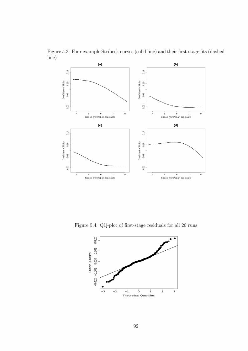
Figure 5.3: Four example Stribeck curves (solid line) and their first-stage fits (dashedline)

4 5 6 7 8

0.02

0.06

0.10

0.14

(a)


Coe

ffici

ent o

f fric

tion

4 5 6 7 8

0.02

0.06

0.10

0.14

(b)


Coe

ffici

ent o

f fric

tion

4 5 6 7 8

0.02

0.06

0.10

0.14

(c)


Coe

ffici

ent o

f fric

tion

4 5 6 7 8

0.02

0.06

0.10

0.14

(d)


Coe

ffici

ent o

f fric

tion

Figure 5.4: QQ-plot of first-stage residuals for all 20 runs

●

●

●

●

●●

●

●

●

●●

●●

●

●●

●

●

●

●

●

●

●

●

●

●

●

●

●

●●

●

●

●

●

●

●

●

●

●

●

●

●●●●

●

●●

●

●

●●

●

●

●●

●●

●

●

●

●

●

●

●

●

●●

●●

●

●

●●

●●

●

●

●●

●

●

●

●

●

●

●

●

●

●

●

●

●●

●

●

●●

●

●●

●●

●

●

●

●

●

●●●

●

●

●

●

●

●

●●

●

●●

●

●

●

●

●●

●●

●●

●●

●

●●●

●

●

●●

●●

●

●●

●●●

●

●●

●●

●

●

●

●

●

●

●

●●

●

●

●

●● ●●● ●

●●●●●

●●

●

●

●●

●

●

●●●

●●●

●●●●

●●●

●

●●

●

●

●●

●●

●

●

●●

●●

●

●

●●

●

●

●

●●

●

●

●

●

●

●

●

●

●

●

●

●

●

●

●

●●

●

●

●

●

●●●

●●

●

●

●

●

●●

●●

●

●

●

●

●

●

●●●

●

●

●

●

●

●

●

●

●

●

●

●

●

●●

●●

●●●

●

●

●

● ●●

●

●●

●●

●●

●

●●

●

●

●

●

●

●

●●

●

●●

●

●

●

●

●

●

●

●

●

●

●

●

●

●

●

●

●●

●

●

●

●

●

●●

●

●

●

●

●

●

●

●

●

●

●

●

●●

●●

●●

●●●

●●●

●●

●

●

●

●

●

●

●

●

●

●

●

●

●●

●

●

●

●●

●

●

●

●

●

●

●

●●●

●●

●

●

●

●

●

●

●

●●

●

●

●

●

●

●

●

●

●

●

●

●

●

●

●

−3 −2 −1 0 1 2 3

−0.0

02−0

.001

0.00

00.

001

0.00

2

Theoretical Quantiles

Sam

ple

Qua

ntile

s

92

vector of unknown coefficients to be estimated from the data and fij is the second

stage error on the loading for the jth principal component for the ith run. The

vector of errors for the ith run, (fi1, fi2, fi3, fi4), is distributed as MVN(0,∆). Note

that this distribution does not depend on i.

All the second stage models were fitted simultaneously using maximum likelihood

estimation. The EM algorithm (Davidian and Giltinan, 1995, pp. 140) was used.

This method allows correlations between the lij and within run variation to be

incorporated. The separate least-squares fits were used as starting values of the

algorithm.

Initially, the model matrix used in the fitting procedure incorporated an intercept

and all main effects. However, from these second stage fits it was apparent that some

interactions were present, particularly involving the process variable roughness. We

needed to select a suitable model from the set of all main effects and two factor inter-

actions (91 parameters in total). Because we have more parameters than runs, the

data set is supersaturated. We therefore turned to a suitable method for analysing

the output of supersaturated experiments. Several methods have been proposed in

the literature, for instance, Westfall et al. (1998) suggested using forward selection,

whilst Beattie et al. (2002) proposed a Bayesian model selection strategy. Further,

Georgiou (2008) gave a method based on orthogonal decomposition. In this chap-

ter, we use the Dantzig selector method, first proposed by Candes and Tao (2007)

and then further explored by Phoa et al. (2009) in the form of the Gauss-Dantzig

selector. Detailed comparisons of certain analysis methods by Marley and Woods

(2010) showed the Gauss-Dantzig selector to be a highly effective method for detect-

ing active effects in supersaturated problems. The Gauss-Dantzig selector is a more

automated procedure than the original Dantzig selector; here we select important

factors through examination of profile plots (see Yuan et al., 2007, for LARs).

The Dantzig selector belongs to a class of continuous variable selection techniques

known as shrinkage methods, where each coefficient is shrunk towards zero at a

different rate. The estimator β is the solution to


93

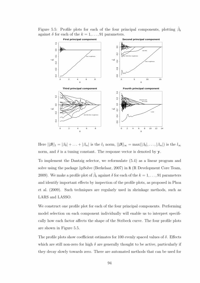
Figure 5.5: Profile plots for each of the four principal components, plotting βk

against δ for each of the k = 1, . . . , 91 parameters.

0 2 4 6 8

−0.4

−0.3

−0.2

−0.1

0.0

0.1

First principal component

δ

β k^

Disc roughness

0 5 10 15

−0.8

−0.6

−0.4

−0.2

0.0

Second principal component

δ

β k^

Disc roughness

Det MG

Det TBN:Disc roughness

0 2 4 6 8

−0.4

−0.2

0.0

0.2

Third principal component

δ

β k^

Det MG:Disc roughness

0 2 4 6 8 10 12 14

−0.6

−0.4

−0.2

0.0

0.2

0.4

Fourth principal component

δ

β k^Load

Disp B:LoadEP:Load

Here ||β||1 = |β0|+ . . .+ |βm| is the l1 norm, ||β||∞ = max(|β0|, . . . , |βm|) is the l∞

norm, and δ is a tuning constant. The response vector is denoted by y.

To implement the Dantzig selector, we reformulate (5.4) as a linear program and

solve using the package lpSolve (Berkelaar, 2007) in R (R Development Core Team,

2009). We make a profile plot of βk against δ for each of the k = 1, . . . , 91 parameters

and identify important effects by inspection of the profile plots, as proposed in Phoa

et al. (2009). Such techniques are regularly used in shrinkage methods, such as

LARS and LASSO.

We construct one profile plot for each of the four principal components. Performing

model selection on each component individually will enable us to interpret specifi-

cally how each factor affects the shape of the Stribeck curve. The four profile plots

are shown in Figure 5.5.

The profile plots show coefficient estimates for 100 evenly spaced values of δ. Effects

which are still non-zero for high δ are generally thought to be active, particularly if

they decay slowly towards zero. There are automated methods that can be used for

94

choosing an optimal δ, such as the AIC statistic or cross validation. Here, we use

visual inspection since we wish to ensure we do not leave out any effects that may

be marginally active. Leaving out an active factor at the screening stage is often less

desired than carrying forward a spurious model term to the follow-up experiment,

since the discarded factor will not be considered again.

For the first principal component there is one line on the plot which clearly corre-

sponds to a significant effect, this being disc roughness. For the second component,

disc roughness also appears to be highly significant (reaching zero at δ ≈ 15), whilst

Det MG and the interaction between Det TBN and disc roughness may also be sig-

nificant (reaching zero at δ ≈ 9 and δ ≈ 5). The third component is less clear, with

no effect being clearly active. However, we retain the variable with consistently the

largest coefficient - the interaction between Det MG and disc roughness. Such an

interaction would be interpretable, since both main effects involved appeared to be

active for the second component. For the fourth component, load was clearly an

active factor, with the interaction between Disp B and load and also between EP

and load being potentially active (both reaching zero at δ ≈ 8).

The terms identified as significant from the profile plots along with the main effects

necessary for effect heredity to be obeyed were used to fit the second stage model.

However, upon examining the fits, it was apparent that the level of bias in some

of the fits was quite strong, see for instance Figure 5.6. Since the first loading on

the first principal component controlled the height of the fitted curve (see Section

5.3.3), we examined further variables that could be marginally significant for the

first principal component. Including the interaction between ZN APHOS and disc

roughness in the model for loadings on the first component reduced the level of bias

in some of the fits and also reduced the overall mean squared error across all of

the runs. Four fits including this interaction and the main effect of ZN APHOS are

shown in Figure 5.7. The dotted lines show the approximate 95% Wald confidence

intervals, as described by Woods (2003, ch. 4). The estimate of the asymptotic

covariance matrix for β is given by Davidian and Giltinan (1995, ch. 5).

Notice how the bias in the fits for curves (a) and (d) has been reduced. All four

of the example fits match the shape of the observed Stribeck curve very well. The

95

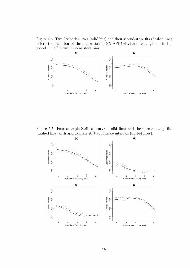
Figure 5.6: Two Stribeck curves (solid line) and their second-stage fits (dashed line)before the inclusion of the interaction of ZN APHOS with disc roughness in themodel. The fits display consistent bias.

4 5 6 7 8

0.02

0.06

0.10

0.14

(a)


Coe

ffici

ent o

f fric

tion

4 5 6 7 8

0.02

0.06

0.10

0.14

(d)


Coe

ffici

ent o

f fric

tion

Figure 5.7: Four example Stribeck curves (solid line) and their second-stage fits(dashed line) with approximate 95% confidence intervals (dotted lines).

4 5 6 7 8

0.02

0.06

0.10

0.14

(a)


Coe

ffici

ent o

f fric

tion

4 5 6 7 8

0.02

0.06

0.10

0.14

(b)


Coe

ffici

ent o

f fric

tion

4 5 6 7 8

0.02

0.06

0.10

0.14

(c)


Coe

ffici

ent o

f fric

tion

4 5 6 7 8

0.02

0.06

0.10

0.14

(d)


Coe

ffici

ent o

f fric

tion

96

Figure 5.8: QQ-plot of scaled second-stage residuals and plot of scaled second-stageresiduals against fitted values

●

●

●

●

●

●

●

●

●

●

●

●

●

●

●

●

●

●

●

●

●

●

●

●●

●

●

● ●●● ●

●

●

●

●●

●

●

●●

●

●●

●

●

●

●

●

●●

●

●

●

●

●

●

●

●

●

●

●●

●

●

●

●

●

●

●

●

●

●

●

●

●

●●

●

●

−2 −1 0 1 2

−2−1

01

2


Sam

ple

Qua

ntile

s●

●

●

●

●

●

●

●

●

●

●

●

●

●

●

●

●

●

●

●

●

●

●

●●

●

●

●● ●● ●

●

●

●

●●

●

●

●●

●

● ●

●

●

●

●

●

●●

●

●

●

●

●

●

●

●

●

●

●●

●

●

●

●

●

●

●

●

●

●

●

●

●

● ●

●

●

−2 −1 0 1 2

−2−1

01

2

Fitted value

Scal

ed re

sidu

al

confidence intervals were judged by subject experts to be narrow enough for the

model to be useful. In the vast majority of the 20 runs, the fitted model captures

very accurately the shape of the curve. Discrepancies between the fitted curve and

the observed curve tend to come in the form of an upward or downward shift. This

is due to the nature of the two-stage fitting procedure. For instance, a small error

in the prediction of the loading for the first principal component will result in an

upward or downward bias (see also Section 5.3.3).

We now examine the residuals for the models fitted for the loadings at the second

stage. Because of potentially unequal variance for the loadings for each component

at the first stage, the residuals were transformed as in Grove et al. (2004) so that

each quadruplet (lij − xiβ), j = 1, . . . , 4 had an approximately multivariate normal

distribution with mean 0 and an identity covariance matrix. Figure 5.8 shows the

QQ-plot of the scaled residuals and also a plot of the scaled residuals against fitted

values; neither plot indicates serious departures from the model assumptions.

5.3.3 Interpretation of the principal components

Figure 5.9 shows plots of the first four principal components. Notice that com-

ponents (i) and (ii) display much more curvature, as they are explaining a higher

proportion of the variation in the shape of the Stribeck curves.

In this section, we describe how to interpret the principal components. For instance,

if a particular factor is significant for a given principal component, we wish to know

how this factor influences the shape of the observed Stribeck curve. We use a similar

97

Figure 5.9: Plots of the first four principal components.

4 5 6 7 8

−0.1

0−0

.06

−0.0

20.

02

(i)


Coe

ffici

ent o

f fric

tion

4 5 6 7 8

−0.1

0−0

.06

−0.0

20.

02

(ii)


Coe

ffici

ent o

f fric

tion

4 5 6 7 8

−0.1

0−0

.06

−0.0

20.

02

(iii)


Coe

ffici

ent o

f fric

tion

4 5 6 7 8

−0.1

0−0

.06

−0.0

20.

02

(iv)


Coe

ffici

ent o

f fric

tion

approach to one described in Campbell et al. (2006); each component is considered

individually, see Figure 5.10. The solid line in Figure 5.10 (i) shows the mean of all

20 observed Stribeck curves. The upper (lower) dashed line is this mean minus (plus)

a small multiple of the first component. This illustrates that the first component

represents the general height of the Stribeck curve, and that variables significant for

this component will change the overall height of the curve. For instance, rough discs

tend to give higher curves than smooth discs.

The solid line in Figure 5.10 (ii) also shows the mean of all 20 observed Stribeck

curves. The convex (concave) dashed line is this mean plus (minus) a small multi-

ple of the second component. The loading on the second component is essentially

determining whether or not we have a concave or convex curve (for example a curve

like in Figure 5.2 (a) or (b)). The variable disc roughness is highly significant for

the second component. Using a rough disc leads to a concave curve and using a

smooth disc leads to a convex curve.

The third principal component is more interpretable when examining the concave

curves (those obtained when using rough discs), hence the solid line in Figure 5.10

98

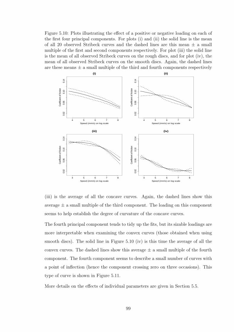
Figure 5.10: Plots illustrating the effect of a positive or negative loading on each ofthe first four principal components. For plots (i) and (ii) the solid line is the meanof all 20 observed Stribeck curves and the dashed lines are this mean ± a smallmultiple of the first and second components respectively. For plot (iii) the solid lineis the mean of all observed Stribeck curves on the rough discs, and for plot (iv), themean of all observed Stribeck curves on the smooth discs. Again, the dashed linesare these means ± a small multiple of the third and fourth components respectively

4 5 6 7 8

0.02

0.06

0.10

0.14

(i)


Coe

ffici

ent o

f fric

tion

4 5 6 7 8

0.02

0.06

0.10

0.14

(ii)


Coe

ffici

ent o

f fric

tion

4 5 6 7 8

0.02

0.06

0.10

0.14

(iii)


Coe

ffici

ent o

f fric

tion

4 5 6 7 8

0.02

0.06

0.10

0.14

(iv)


Coe

ffici

ent o

f fric

tion

(iii) is the average of all the concave curves. Again, the dashed lines show this

average ± a small multiple of the third component. The loading on this component

seems to help establish the degree of curvature of the concave curves.

The fourth principal component tends to tidy up the fits, but its sizable loadings are

more interpretable when examining the convex curves (those obtained when using

smooth discs). The solid line in Figure 5.10 (iv) is this time the average of all the

convex curves. The dashed lines show this average ± a small multiple of the fourth

component. The fourth component seems to describe a small number of curves with

a point of inflection (hence the component crossing zero on three occasions). This

type of curve is shown in Figure 5.11.

More details on the effects of individual parameters are given in Section 5.5.

99

Figure 5.11: An observed Stribeck curve with a point of inflection.

4 5 6 7 8

0.02

0.06

0.10

0.14

(e)


Coef

ficie

nt o

f fric

tion

5.4 Choosing follow-up runs

After the screening stage of the experiment, resource was available for 10 follow-up

runs to help improve the model. In this section, we first describe the theory behind

generating these follow-up runs, and then detail the actual runs used in the Stribeck

curve example.

5.4.1 Theory

We first express the models we have fitted in matrix form. At the first-stage we

fitted the model

Yi =4∑

j=1

Djlij + Ei .

In matrix form, this can be written as

Y = [YT1 , . . . ,Y

T20]

T = (I20 ⊗D)L + E , (5.5)

where, I20 is the 20×20 identity matrix, D is the 21×4 matrix with the four principal

components as the columns. We have E = [ET1 , . . . ,E

T20]

T and set L = [L1, . . . ,L20]T ,

where Li is the 1× 4 vector of loadings for the ith run.

We let β = [β1, . . . ,β4]T , where βj is a 1 × p vector containing the coefficients for

the loadings for the jth principal component and p is the total number of effects

100

under investigation. We use the notation Xi = I4 ⊗ xi, where xi is the 1× p model

matrix for the ith run, and let

X∗ =

[X1

...X20

].

At the second stage, we then fit the model

L = X∗β + F , (5.6)

where F is a 80× 1 vector of errors.

Combining (5.5) and (5.6) we get

Y = (I20 ⊗D)X∗β + (I20 ⊗D)F + E ,

where F ∼MVN(0,ΣF ), with ΣF = I20⊗∆, and E ∼MVN(0,Σ), with Σ = σI420.

From the theory of generalised least squares, the information matrix is given by

X∗T (I20 ⊗DT )[(I20 ⊗D)ΣF (I20 ⊗DT ) + Σ]−1(I20 ⊗D)X∗ .

When designing the follow-up experiment, we wish to choose runs such that the

determinant of the information matrix given the initial batch of runs is maximised.

Let X∗e be the model matrix for all the runs in the experiment (screening and follow-

up) consisting of all the parameters found to be active, or at least, potentially active

at the screening stage. The first 20 runs of X∗e are fixed and we wish to choose the

remaining 10 to maximise

φ(2)D = |X∗Te (I30 ⊗DT )[(I30 ⊗D)ΣF (I30 ⊗DT ) + Σ]−1(I30 ⊗D)X∗e| . (5.7)

We use the best estimate of the basis (i.e., that from the screening stage) for gener-

ating the follow-up design. We extend the covariance matrices to be ΣF = I30 ⊗∆

and Σ = σI630 and estimate ∆ and σ from the data from the screening stage. Such

an approach makes best use of information from screening stage when generating

the follow-up runs.

101

Table 5.6: Percentages of each ingredient and settings of the two process variablesin the 10-run follow-up design

Run ZDP3 Det1 Det2 Det3 Disp1 EP1 Load (N) Roughness1 0.48 0 0 3 2 0 72 Smooth2 0.48 0 0 3 2 0.1 72 Rough3 0 0 0 0 2 0 72 Rough4 0.48 0 0 0 2 0 37 Smooth5 0 0 0 3 2 0.1 37 Smooth6 0.48 3 0 0 2 0.1 37 Smooth7 0.48 0 0 0 0 0 37 Rough8 0.48 3 0 0 2 0.1 72 Rough9 0.48 0 0 3 0 0.1 72 Smooth10 0 0 0 0 0 0 72 Smooth

5.4.2 Experimental design for 10 follow-up runs

For the follow-up runs, there were no constraints on the total number of oils that

could be used. A total of 7 factors out of the initial 13 were retained, along with 5

interactions, see Section 5.3.2. The 10 follow-up runs were generated using a similar

algorithm to the one described in Section 5.2 to maximise the objective function

(5.7). The matrix giving the weights for the ingredients and the settings of the

process variables for the follow-up runs is given in Table 5.6.

The amount of the ingredients that did not influence levels of any of the factors

retained for the follow-up runs was zero for all runs, except for the amount of

antiwear. This was set so that the minimum required level of phosphorous was

always achieved, in line with constraint 3. Notice that the columns for the two

process variables are now balanced, when the 30 runs are considered as a whole.

We also note that Detergent 2 is never included in the oil. This is because we can

achieve a higher level of the factor Det TBN combined with a low/high level of Det

MG by using Detergent 1 or 3.

The resulting scaled design is shown in Table 5.7. The follow-up design places the

factor ZN APHOS at its high level more times than in the screening experiment,

which overall makes the column more balanced. It is possible to do this now that

we are only considering one ZDP in the follow-up design (since ZDP1 and ZDP2 do

not affect the levels of any of the factors retained for the follow-up experiment). We

102

Table 5.7: Design matrix for 10-run follow-up experiment. All variables are scaledto lie in the region [-1,1]. Rough discs are coded 1 and smooth discs -1.

Run ZN APHOS Det MG Det TBN Disp B EP Load Roughness1 1 1 1 1 -1 1 -12 1 1 1 1 1 1 13 -1 -1 -1 1 -1 1 14 1 -1 -1 1 -1 -1 -15 -1 1 1 1 1 -1 -16 1 -0.99 1 1 1 -1 -17 1 -1 -1 -1 -1 -1 18 1 -0.99 1 1 1 1 19 1 1 1 -1 1 1 -110 -1 -1 -1 -1 -1 1 -1

see a similar trend with the level of Disp B.

5.5 Results of follow-up runs

The 10 runs shown in Table 5.7 were randomised and the experiment carried out.

The predictions based on the model obtained from the initial 20 runs were compared

to the curves observed in the 10 follow-up runs. They were found to fit well, except

for run 5, which produced an unexpectedly high curve. A repeat was run and the

observed Stribeck curve was closer to the prediction in terms of shape, but still

decidedly biased. The larger than expected bias could be due to the MTM receiving

its annual calibration between the follow-up runs and the repeat. Due to this bias,

run 5 was excluded from the analysis.

The principal components were recalculated for the remaining 29 runs and plotted

as the dashed line in Figure 5.12. The solid line shows the principal components

based on the first 20 runs. For components i and iii (where the dashed line is masked

by the solid line) we see very little change between 20 and 29 runs. For components

ii and iv, the component from 29 runs is virtually exactly the 20 run component

multiplied by minus one (shown by the dotted line overlapping the solid line). Thus

the components are virtually identical, with the interpretation of the direction of

the effects reversed for components ii and iv. We use the components from the full

103

Figure 5.12: Plots of the first four principal components based on 20 (solid) and29 (dashed) runs. For components ii and iv, the dotted line shows the componentbased on 29 runs multiplied by minus one.

4 5 6 7 8

−0.1

0−0

.06

−0.0

20.

02

(i)


Coe

ffici

ent o

f fric

tion

4 5 6 7 8

−0.1

0−0

.06

−0.0

20.

02

(ii)


Coe

ffici

ent o

f fric

tion

4 5 6 7 8

−0.1

0−0

.06

−0.0

20.

02

(iii)


Coe

ffici

ent o

f fric

tion

4 5 6 7 8

−0.1

0−0

.06

−0.0

20.

02

(iv)


Coe

ffici

ent o

f fric

tion

29 runs for the remainder of the analysis.

Second stage models were estimated for all 29 curves, using all the effects carried

forward to the follow-up experiment. All 12 of these effects could be argued as being

at least potentially active for some principal components, based on examining box-

plots of the loadings. Therefore, it was difficult to reduce the number of parameters

in the model. The most obviously active effects were disc roughness, load and the

interactions between Det MG and disc roughness and Det TBN and disc roughness.

Fitting a model in these effects and also the main effects of Det MG and Det TBN

(to obey effect heredity) resulted in an increase in mean squared error of 248%,

strongly indicating that the remaining effects were appreciably improving the fit.

The residual plots shown in Figure 5.13 show no discernible patterns or deviations

from normality. The points indicated by a cross symbol denote those relating to the

follow-up runs. There is no detectable difference between the follow-up runs and

the screening runs.

104

Figure 5.13: QQ-plot of scaled second-stage residuals and plot of scaled second-stageresiduals against fitted values based on 29 runs. Circular points correspond to runs1-20 and crosses correspond to the nine retained follow-up runs.

●

●

●

●

●

●

●

●

●

●

●

●

●

●

●

●

●

●

●

●

●

●

●●●

●

●

●

●

●

●

●

●

●

●

●

●

●

●

●

●

●

●

●●

●

●

●●

●

●

●

●

●

●

●

●

●●

●

●

●

●

●

●

●

●

●

●

●

●

●

●

●

●

●

●

●●

●

●

−2 −1 0 1 2

−4−2

02


Stan

dard

Qua

ntile

s

●

●

●

●

●

●

●

●

●

●

●

●

●

●

●

●

●

●

●

●

●

●

● ●●

●

●

●

●

●

●

●

●

●

●

●

●

●

●

●

●

●

●

●●

●

●

●●

●

●

●

●

●

●

●

●

●●

●

●

●

●

●

●

●

●

●

●

●

●

●

●

●

●

●

●

●●

●

−1.5 −1.0 −0.5 0.0 0.5 1.0 1.5

−4−2

02

Fitted value

Scal

ed re

sidu

al

We now examine graphically the effects of changing some of the factor levels. Figure

5.14 (left) shows the estimated effect on the Stribeck curve of changing the level of

Det MG from -0.99 (dashed line) to 1 (solid line) when a smooth disc is being used

and all other factors are kept constant. Figure 5.14 (right) shows the corresponding

effect when a rough disc is being used. The difference between the curves is much

greater when a rough disc is used, due to the substantive interaction between Det

MG and disc roughness.

We also examine the effect of changing load from low to high. Load was active

only for the fourth principal component, which explained only a small amount of

the variation in the shape of the Stribeck curves. Therefore, Figure 5.15 shows only

small differences between the estimated curves for low and high load.

Disp B was included in the model due to it’s interaction with load. The plots in

the upper row of Figure 5.16 show that, at a high load, Disp B is likely to have

little effect on the shape of the Stribeck curve. However, at low loads (plots in the

bottom row of Figure 5.16) the difference is more noticeable, with a lower level of

Disp B appearing to produce lower curves at low speeds.

5.6 Discussion

We have described the statistical methodology behind an investigation into the effect

of certain factors on the shape of Stribeck curves. The models that were estimated

during this work and the graphical displays of anticipated effects of changing various

105

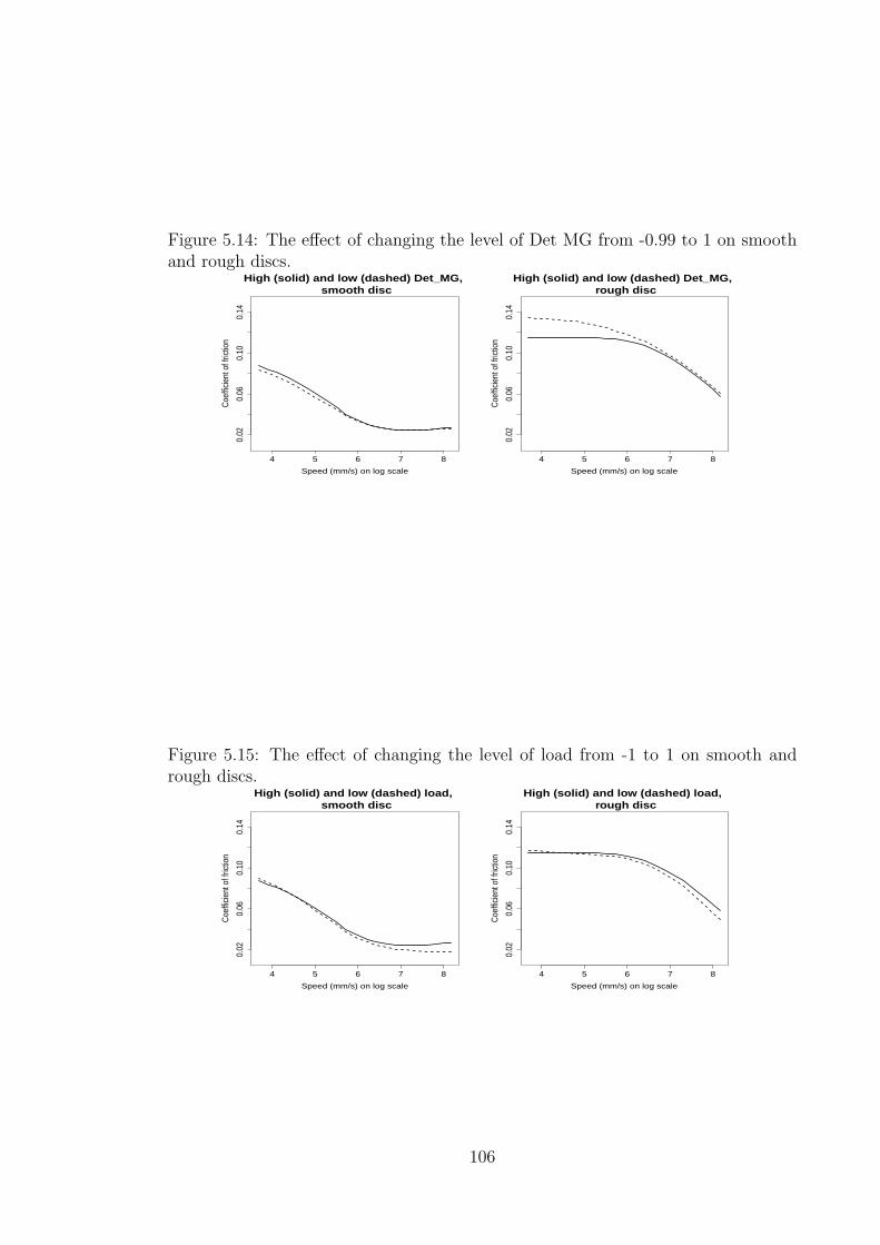
Figure 5.14: The effect of changing the level of Det MG from -0.99 to 1 on smoothand rough discs.

4 5 6 7 8

0.02

0.06

0.10

0.14

High (solid) and low (dashed) Det_MG, smooth disc


Coe

ffici

ent o

f fric

tion

4 5 6 7 8

0.02

0.06

0.10

0.14

High (solid) and low (dashed) Det_MG, rough disc


Coe

ffici

ent o

f fric

tion

Figure 5.15: The effect of changing the level of load from -1 to 1 on smooth andrough discs.

4 5 6 7 8

0.02

0.06

0.10

0.14

High (solid) and low (dashed) load, smooth disc


Coe

ffici

ent o

f fric

tion

4 5 6 7 8

0.02

0.06

0.10

0.14

High (solid) and low (dashed) load, rough disc


Coe

ffici

ent o

f fric

tion

106

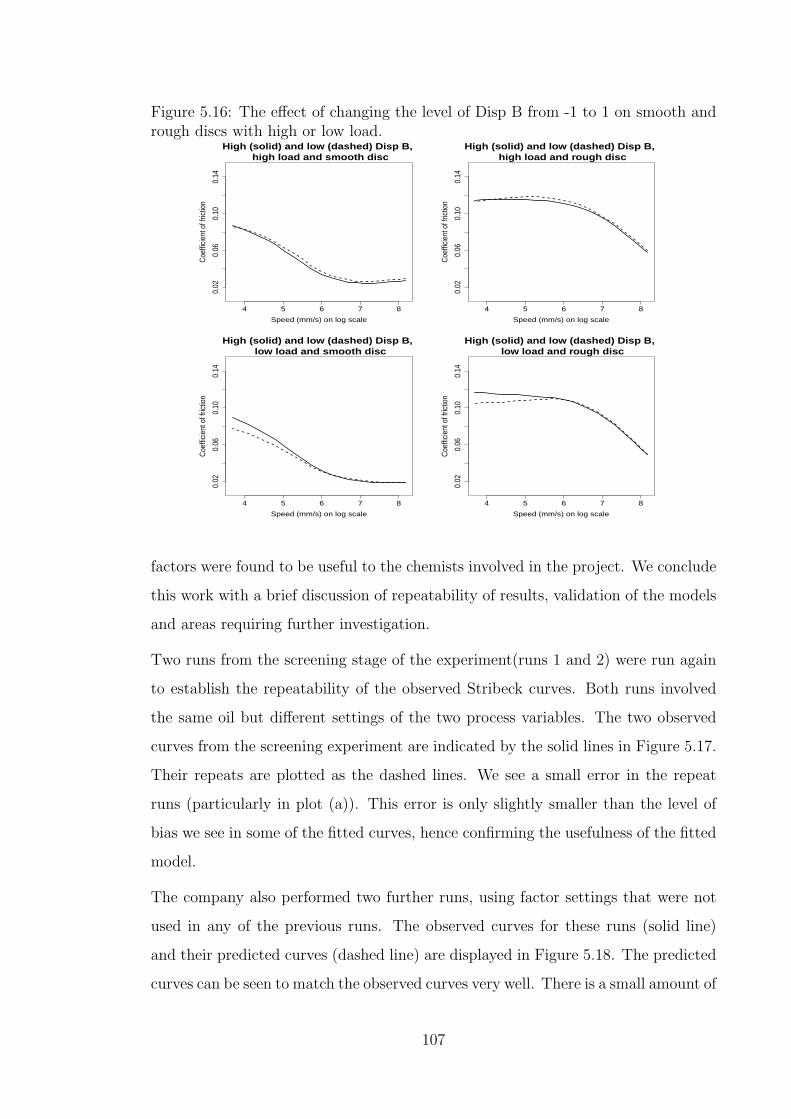
Figure 5.16: The effect of changing the level of Disp B from -1 to 1 on smooth andrough discs with high or low load.

4 5 6 7 8

0.02

0.06

0.10

0.14

High (solid) and low (dashed) Disp B, high load and smooth disc


Coe

ffici

ent o

f fric

tion

4 5 6 7 8

0.02

0.06

0.10

0.14

High (solid) and low (dashed) Disp B, high load and rough disc


Coe

ffici

ent o

f fric

tion

4 5 6 7 8

0.02

0.06

0.10

0.14

High (solid) and low (dashed) Disp B, low load and smooth disc


Coe

ffici

ent o

f fric

tion

4 5 6 7 8

0.02

0.06

0.10

0.14

High (solid) and low (dashed) Disp B, low load and rough disc


Coe

ffici

ent o

f fric

tion

factors were found to be useful to the chemists involved in the project. We conclude

this work with a brief discussion of repeatability of results, validation of the models

and areas requiring further investigation.

Two runs from the screening stage of the experiment(runs 1 and 2) were run again

to establish the repeatability of the observed Stribeck curves. Both runs involved

the same oil but different settings of the two process variables. The two observed

curves from the screening experiment are indicated by the solid lines in Figure 5.17.

Their repeats are plotted as the dashed lines. We see a small error in the repeat

runs (particularly in plot (a)). This error is only slightly smaller than the level of

bias we see in some of the fitted curves, hence confirming the usefulness of the fitted

model.

The company also performed two further runs, using factor settings that were not

used in any of the previous runs. The observed curves for these runs (solid line)

and their predicted curves (dashed line) are displayed in Figure 5.18. The predicted

curves can be seen to match the observed curves very well. There is a small amount of

107

Figure 5.17: Observed Stribeck curves for runs 1 and 2 (a and b) from the screeningstage (solid lines) and their repeats (dashed lines)

4 5 6 7 8

0.02

0.06

0.10

0.14

(a)


Coe

ffici

ent o

f fric

tion

4 5 6 7 8

0.02

0.06

0.10

0.14

(b)


Coe

ffici

ent o

f fric

tion

Figure 5.18: Observed Stribeck curves from two validation runs (solid lines) andtheir predicted curves (dashed lines)

4 5 6 7 8

0.02

0.06

0.10

0.14

(a)


Coe

ffici

ent o

f fric

tion

4 5 6 7 8

0.02

0.06

0.10

0.14

(b)


Coe

ffici

ent o

f fric

tion

bias evident in curve (a) but this is not too much larger than the errors seen between

repeat runs in Figure 5.17. We note, however, that there are limited conclusions

that can be drawn from only two validation runs and that more validation runs

would give us more confidence in the fitted model.

Discussion with researchers at Lubrizol revealed that the small amounts of bias

seen in the fitted curves could be due to some discs being slightly more rough or

smooth than others, even within their respective groups. Roughness of the discs can

be quantified by calculating different summary measures from a roughness profile,

a plot of depth measurements obtained by running a stylus across a portion of

the disc. Two useful measurements which were identified were Ra, the average

absolute deviation from the mean line of the measurements in the profile, and Rsk,

the skewness of the profile measurements. Roughness profiles were taken in three

positions on all discs prior to experimentation but were found to vary considerably

108

within the same disc. Consequently, it was not possible to accurately characterise

disc roughness using Ra and Rsk. Models were fitted using Ra instead of a two-level

disc roughness factor, but these were found to provide a less accurate fit to the

data, along with wider confidence intervals. Obtaining better ways to measure disc

roughness is the subject of further investigation.

It should be noted that, ideally, the experimenters would have anticipated a small

number of strong two-factor interactions, and the screening experiment could then

have been designed with the model matrix, X also incorporating two-factor inter-

actions. This would then be a supersaturated design problem, with there being

more parameters to be investigated than runs available in the experiment. Bayesian

D-optimality (Jones et al., 2008) could potentially have been used as a suitable

criterion.

We also point out that if, at the screening stage of the experiment, we had more

runs available than observations per Stribeck curve, then the whole experiment

could, under some assumptions, be designed in the framework described in Section

5.4. Suppose there are q points which make up each Stribeck curve and that q < n.

Let’s assume that we will select all principal components to form our basis, so that

E = 0 (i.e. no first stage errors). Also assume that the loadings are uncorrelated.

Then ΣF = In×q. The objective function to find the 20 screening runs becomes

|XT (I20 ⊗DT )[(I20 ⊗D)(I20 ⊗DT )]−1(I20 ⊗D)X| .

Since we are using all available principal components, D is a q × q square matrix

and hence the objective function reduces to

|XT X| .

Even though in the example considered in this chapter we have q > n, maximising

|XT X| is still a sensible option, particularly since we do not know the principal

components in advance.

Lubrizol were particularly encouraged by the findings of this experiment, and there

are now plans for them to apply this methodology to other similar projects.

109

Chapter 6

Overall conclusions and futurework

This thesis has discussed industrial screening experiments and has provided new

methods and insights for the design and analysis of supersaturated experiments.

The performance of the supersaturated designs has been evaluated by calculating the

power and type I error rate across a variety of simulation studies. New applications

of supersaturated experiments have been presented. These include supersaturated

experiments where factor levels cannot be set independently, and robust product

design via supersaturated experiments. Finally a real-life screening experiment run

by The Lubrizol Corporation to investigate the influence of factors on friction, rep-

resented by Stribeck curves was discussed. This example involved the development

of a new method of selecting follow-up designs for two-stage models.

6.1 Conclusions

Results of a detailed simulation study have enabled recommendations to be made for

the successful application of supersaturated designs. The recommendation of most

potential use to practitioners is that the number of factors should not normally

exceed twice the number of runs. The study also showed that, despite often being

unbalanced, Bayesian D-optimal designs can perform well, and tend to have slightly

higher power in return for a slightly higher type I error rate when compared to

E(s2)-optimal designs.

A suitable method for analysing the results of supersaturated experiments has also

110

been identified. Compared to two other existing methods the Gauss-Dantzig selector

had consistently higher power and also a low type I error rate across a range of

scenarios and experiment sizes. The Gauss-Dantzig selector also performed better

than a newly proposed model-averaging procedure.

Advances have also been made in the design of supersaturated experiments. A

compound criterion has been proposed for designing supersaturated experiments

that facilitates the construction of designs with both low levels of multicollinearity

and good accuracy of parameter estimators. The criterion maximises an objective

function that combines the average variance inflation factor with a modification

of the A-optimality objective function. This criterion is different to the majority

of existing criteria in that it considers projections into more than two factors. It

also has the advantage that all models containing up to a pre-specified number

of factors can be estimated. In principal it can be used for constructing designs

for any number of runs and factors. This new criterion can be especially effective

for experiments where the levels of the factors cannot be set independently of one

another. Reducing multicollinearity is useful in such experiments, since there may

be inherent relationships between the factors in the candidate list of design points.

Therefore we recommend using this criterion for such experiments.

It has been demonstrated that to which columns of a supersaturated design the

active factors are assigned can have a considerable impact on the ability to detect

those factors in the analysis. Investigation revealed that for a given design, active

factors assigned to columns with high average variance inflation factors were far

more likely to be declared inactive in the analysis compared to those assigned to

columns with low variance inflation factors. It was therefore suggested that exper-

imenters may wish to consider this issue, and assign factors to columns carefully,

using any available prior information. A method for doing this was proposed, which

involved assigning the factors using the average variance inflation factor for individ-

ual columns of the design.

One especially useful application of screening in industry is in the context of robust

product design experiments and it has been shown that supersaturated designs can

be very effective for this problem. Using a criterion which is focussed only on the

111

aliasing structure for effects of interest proved more effective than using existing

criteria for constructing such designs. Large improvements in the power to detect

active factors can be gained, especially when there are more noise factors than

control factors. Often, potential noise factors (and hence potential control by noise

interactions) are ignored in such experiments, because noise factors can be expensive

to vary in experiments. The implementation of supersaturated designs can enable

more noise factors to be investigated and hence improve products further. The

criterion proposed in Chapter 4 is also generalisable outside of the robust parameter

design setting to applications where there is a set of effects which is of interest and

a set which is not.

The work in this thesis was strongly motivated by interactions with industry and

Chapter 5 described a real screening experiment to investigate the impact of factors

on functional responses, namely Stribeck curves. Designing the experiment using a

candidate list approach and analysing via a two-stage model, with principal compo-

nents analysis used at the first stage, proved to be effective. Several active factors

were identified, and accurate models for the Stribeck curves were obtained. A novel

method for constructing a follow-up experiment was described and implemented.

6.2 Future work

There are a variety of open issues and areas of future work resulting from this thesis.

In Chapter 2 we could include a Bayesian analysis method in the comparisons, such

as the two-stage model selection strategy proposed by Beattie et al. (2002). The

comparisons could also be extended to scenarios where we also aim to detect active

two-factor interactions.

In order to speed up generation of the designs using the compound criterion de-

scribed in Chapter 3, and to enable the generation of larger designs, it would be

beneficial to develop updating formulae for the objective function when an exchange

or coordinate exchange algorithm is being used. This would ideally avoid the in-

version of the large number of matrices currently required, which could result in

computational savings. As an example, Atkinson et al. (2007, ch. 12) present a re-

peated application of the Sherman-Morrison formula (Sherman and Morrison, 1950)

112

for when D-optimality is being used as the criterion. It is, however, unclear what

savings in computer time would be possible for the objective function in Chapter

3, since the matrices to be inverted are typically small. As a further extension, the

criterion in Chapter 3 could also be applied to models with interactions.

For the example in Chapter 5, it may be possible to create a candidate-list-free

continuous optimisation approach to generate the optimal elements of the weight

matrix W. This will most likely be more computationally intensive, but would have

the advantage of being a more general method.

Additional work could involve investigating screening experiments for more compli-

cated models. This thesis has described screening experiments for only main effects

and, in some cases, two-factor interactions. For some experiments, modelling the

response may require more complex functions of the controllable factors, for example

quadratic effects or spline bases, for which new methodology may be required.

113

References

Abraham, B., Chipman, H., and Vijayan, K. (1999), “Some risks in the construction

and analysis of supersaturated designs,” Technometrics, 41, 135–141.

Allen, T. T. and Bernshteyn, M. (2003), “Supersaturated designs that maximise the

probability of identifying active factors,” Technometrics, 45, 90–97.

Aston, J. A. D., Chiou, J.-M., and Evans, J. P. (2010), “Linguistic pitch analysis

using functional principal component mixed effect models,” Journal of the Royal

Statistical Society Series C, 59, 297–317.

Atkinson, A. C., Donev, A. N., and Tobias, R. D. (2007), Optimum experimental

designs, with SAS, Oxford: Oxford University Press.

Ballistreri, F. P., Fortuna, C. G., Musumarra, G., Pavone, D., and Scire, S. (2002),

“Principal properties (PPs) as solvent descriptors for multivariate optimization in

organic synthesis: specific PPs for ethers,” Arkivoc, 11, 54–64.

Beattie, S. D., Fong, D. K. H., and Lin, D. K. J. (2002), “A two-stage Bayesian

model selection strategy for supersaturated designs,” Technometrics, 44, 55–63.

Berkelaar, M. (2007), lpSolve: Interface to Lp solve v. 5.5 to solve linear/integer

programs.

Booth, K. H. V. and Cox, D. R. (1962), “Some systematic supersaturated designs,”

Technometrics, 4, 489–495.

Box, G. E. P. (1959), “Discussion of the papers of Satterthwaite and Budne,” Tech-

nometrics, 1, 174–180.

114

Box, G. E. P. and Meyer, R. D. (1986), “An analysis for unreplicated fractional

factorials,” Technometrics, 28, 11–18.

Burnham, K. P. and Anderson, D. R. (2002), Model selection and multimodel infer-

ence, New York, London: Springer, 2nd ed.

Campbell, K., McKay, M. D., and Williams, B. J. (2006), “Sensitivity analysis

when model outputs are functions,” Reliability Engineering and System Safety,

91, 1468–1472.

Candes, E. and Tao, T. (2007), “The Dantzig selector: statistical estimation when

p is much larger than n,” The Annals of Statistics, 35, 2313–2351.

Chen, J. and Liu, M. Q. (2008), “Optimal mixed-level supersaturated design with

general number of runs,” Statistics and Probability Letters, 78, 2496–2502.

Cook, R. D. and Nachtsheim, C. J. (1980), “A comparison of algorithms for con-

structing exact D-optimal designs,” Technometrics, 22, 315–324.

Crosier, R. B. (2000), “Some new two-level saturated designs,” Journal of Quality

Technology, 32, 103–110.

Davidian, M. and Giltinan, D. M. (1995), Nonlinear models for repeated measure-

ment data, London: Chapman and Hall.

Dean, A. M. and Lewis, S. M. (2006), Screening: methods for experimentation in

industry, drug discovery, and genetics, New York: Springer.

Deng, L. Y., Lin, D. K. J., and Wang, J. (1996), “A measurement of multi-factor

orthogonality,” Statistics & Probability Letters, 28, 203–209.

Dowson, D. (1998), History of tribology, 2nd ed., London and Bury St Edmunds:

Professional Engineering Publishing.

DuMouchel, W. and Jones, B. (1994), “A simple Bayesian modification of D-optimal

designs to reduce dependence on an assumed model,” Technometrics, 36, 37–47.

Georgiou, S. D. (2008), “Modelling by supersaturated designs,” Computational

Statistics and Data Analysis, 53, 428–435.

115

Gilmour, S. G. (2006), “Supersaturated designs in factor screening,” in Screening:

methods for experimentation in industry, drug discovery, and genetics, eds. Dean,

A. M. and Lewis, S. M., New York: Springer, pp. 169–190.

Grove, D. M., Woods, D. C., and Lewis, S. M. (2004), “Multifactor B-spline mixed

models in designed experiments for the engine mapping problem,” Journal of

Quality Technology, 36, 380–391.

Holcomb, D. R., Montgomery, D. C., and Carlyle, W. M. (2007), “The use of super-

saturated experiments in turbine engine development,” Quality Engineering, 19,

17–27.

Jolliffe, I. T. (2002), Principal component analysis, New York: Springer, 2nd ed.

Jones, B., Lin, D. K. J., and Nachtsheim, C. J. (2008), “Bayesian D-optimal super-

saturated designs,” Journal of Statistical Planning and Inference, 138, 86–92.

Jones, B. and Nachtsheim, C. J. (2009), “D-Efficient designs with minimal aliasing,”

Tech. rep., University of Minnesota.

Jones, B. A., Li, W., Nachtsheim, C. J., and Ye, K. Q. (2009), “Model-robust super-

saturated and partially supersaturated designs,” Journal of Statistical Planning

and Inference, 139, 45–53.

Kang, L. and Joseph, V. R. (2009), “Bayesian optimal single arrays for robust

parameter design,” Technometrics, 51, 250–261.

Lauter, E. (1974), “Experimental design in a class of models,” Mathematische Op-

erationsforschung und Statistik, 5, 379–398.

Lewis, S. M. and Dean, A. M. (2001), “Detection of interactions in experiments on

large numbers of factors,” Journal of the Royal Statistical Society Series B, 63,

633–672.

Li, P., Zhao, S., and Zhang, R. (2010), “A cluster analysis selection strategy for

supersaturated designs,” Computational Statistics and Data Analysis, 54, 1605–

1612.

116

Li, R. and Lin, D. K. J. (2002), “Data analysis in supersaturated designs,” Statistics

& Probability Letters, 59, 135–144.

— (2003), “Analysis methods for supersaturated design: some comparisons,” Jour-

nal of Data Science, 1, 249–260.

Li, W. W. and Wu, C. F. J. (1997), “Columnwise-pairwise algorithms with applica-

tions to the construction of supersaturated designs,” Technometrics, 39, 171–179.

Lin, D. K. J. (1993), “A new class of supersaturated designs,” Technometrics, 35,

28–31.

— (1995), “Generating systematic supersaturated designs,” Technometrics, 37, 213–

225.

— (1998), “Spotlight interaction effects in main-effect plans: a supersaturated design

approach,” Quality Engineering, 11, 133–139.

Liu, M. Q. and Lin, D. K. J. (2009), “Construction of optimal mixed-level super-

saturated designs,” Statistica Sinica, 19, 197–211.

Liu, Y., Ruan, S., and Dean, A. M. (2007), “Construction and analysis of Es2

efficient supersaturated designs,” Journal of Statistical Planning and Inference,

137, 1516–1529.

Loeppky, J. L., Bingham, D., and Sitter, R. (2006), “Constructing non-regular ro-

bust parameter designs,” Journal of Statistical Planning and Inference, 136, 3710–

3729.

Lu, X., Khonsari, M. M., and Gelinck, E. R. M. (2006), “The Stribeck curve: exper-

imental results and theoretical prediction,” Journal of Tribology, 128, 789–794.

Madigan, D. and Raftery, A. E. (1994), “Model selection and accounting for model

uncetainty in graphical models using Occam’s window,” Journal of the American

Statistical Association, 89, 1535–1546.

Marley, C. J. and Woods, D. C. (2010), “A comparison of design and model se-

lection methods for supersaturated experiments,” Computational Statistics and

Data Analysis, 54, 3158–3167.

117

Meyer, R. D., Steinberg, D. M., and Box, G. (1996), “Follow-up designs to resolve

confounding in multifactor experiments,” Technometrics, 38, 303–313.

Meyer, R. K. and Nachtsheim, C. J. (1995), “The coordinate-exchange algorithm

for constructing exact optimal experimental designs,” Technometrics, 37, 60–69.

Miller, A. (2002), Subset selection in regression, Boca Raton: Chapman and Hall.

Miller, A., Sitter, R. R., Wu, C. F. J., and Long, D. (1993), “Are large Taguchi-style

experiments necessary? A reanalysis of gear and pinion data,” Quality Engineer-

ing, 6, 21–37.

Morris, M. D. (2006), “An overview of group factor screening,” in Screening: meth-

ods for experimentation in industry, drug discovery, and genetics, eds. Dean, A. M.

and Lewis, S. M., New York: Springer, pp. 191–206.

Neter, J., Kutner, M. H., Nachtsheim, C. J., and Wasserman, W. (1996), Applied

statistical linear models, Chicago: The McGraw-Hill Companies, Inc., 4th ed.

Nguyen, N. K. (1996), “An algorithmic approach to constructing supersaturated

designs,” Technometrics, 38, 69–73.

Nguyen, N. K. and Cheng, C. S. (2008), “New E(s2)-optimal supersaturated designs

constructed from incomplete block designs,” Technometrics, 50, 26–31.

O’Hagan, A. and Forster, J. J. (2004), Kendall’s advanced theory of statistics Vol.

2B: Bayesian Inference, London: Arnold, 2nd ed.

Phoa, F. K. H., Pan, Y. H., and Xu, H. (2009), “Analysis of supersaturated designs

via the Dantzig selector,” Journal of Statistical Planning and Inference, 139, 2362–

2372.

Plackett, R. L. and Burman, J. P. (1946), “The design of optimum multifactorial

experiments,” Biometrika, 33, 305–325.

Put, R., Xu, Q. S., Massart, D. L., and Vander Heyden, Y. (2004), “Multivariate

adaptive regression splines (MARS) in chromatographic quantitative structure-

retention relationship studies,” Journal of Chromatography A, 1055, 11–19.

118

R Development Core Team (2009), R: A language and environment for statistical

computing, R Foundation for Statistical Computing, Vienna, Austria.

Ramsay, J. O. and Silverman, B. W. (2005), Functional data analysis, New York:

Springer, 2nd ed.

Russell, K. G., Lewis, S. M., and Dean, A. M. (2004), “Fractional factorial designs

for the detection of interactions between design and noise factors,” Journal of

Applied Statistics, 31, 545–552.

Ryan, K. J. and Bulutoglu, D. A. (2007), “E(s2)-optimal supersaturated designs

with good minimax properties,” Journal of Statistical Planning and Inference,

137, 2250–2262.

Satterthwaite, F. (1959), “Random balance experimentation,” Technometrics, 1,

111–137.

Sherman, J. and Morrison, W. J. (1950), “Adjustment of an inverse matrix corre-

sponding to a change in one element of a given matrix,” Annals of Mathematical

Statistics, 21, 124–127.

Shoemaker, A. C., Tsui, K. L., and Wu, C. F. J. (1991), “Economical experimenta-

tion methods for robust design,” Technometrics, 33, 415–427.

Snee, R. D. (1973), “Techniques for the analysis of mixture data,” Technometrics,

15, 517–528.

Sojoudi, H. and Khonsari, M. M. (2010), “On the behavior of friction in lubricated

point contact with provision for surface roughness,” Journal of Tribology, 132,

012102.

Srivastava, J. N. (1975), “Designs for searching non-negligible effects,” in A survey

of statistical design and linear models, ed. Srivastava, J. N., Amsterdam: North-

Holland Publishing Co., pp. 507–519.

Stribeck, R. (1902), “Kugellager fur beliebige belastungen,” Zeitschrift des Vereines

Deutscher Ingenieure, 46, 1341–1348; 1432–1438; 1463–1470.

119

Taguchi, G. (1986), Introduction to quality engineering: designing quality into prod-

ucts and processes, Tokyo: Asian Productivity Organization.

Vine, A. E., Lewis, S. M., Dean, A. M., and Brunson, D. (2008), “A critical assess-

ment of two-stage group screening through industrial experimentation,” Techno-

metrics, 50, 15–25.

Watson, G. S. (1961), “A study of the group screening method,” Technometrics, 3,

371–388.

Welch, W. J., Yu, T. K., Kang, S. M., and Sacks, J. (1990), “Computer experiments

for quality control by parameter design,” Journal of Quality Technology, 22, 15–

22.

Westfall, P. H., Young, S. S., and Lin, D. K. J. (1998), “Forward selection error

control in the analysis of supersaturated designs,” Statistica Sinica, 8, 101–117.

Woods, D. C. (2003), “Designing experiments for polynomial spline models,” Ph.D.

thesis, University of Southampton.

Wu, C. F. J. (1993), “Construction of supersaturated designs through partially

aliased interactions,” Biometrika, 80, 661–669.

Wu, C. F. J. and Hamada, M. (2000), Experiments: Planning, Analysis, and Pa-

rameter Design Optimization, New York: Wiley.

Wu, C. F. J. and Zhu, Y. (2003), “Optimal selection of single arrays for parameter

design experiments,” Statistica Sinica, 13, 1179–1199.

Xu, H. and Wu, C. F. J. (2005), “Construction of optimal multi-level supersaturated

designs,” The Annals of Statistics, 33, 2811–2836.

Yamada, S. and Lin, D. K. J. (1999), “Three-level supersaturated designs,” Statistics

& Probability Letters, 45, 31–39.

Yuan, M., Joseph, V. R., and Lin, Y. (2007), “An efficient variable selection approach

for analyzing designed experiments,” Technometrics, 49, 430–439.

120

Zhu, Y., Zeng, P., and Jennings, K. (2007), “Optimal compound orthogonal arrays

and single arrays for robust parameter design experiments,” Technometrics, 49,

440–453.

121

university of southampton research repository … of southampton abstract faculty of social and...

Documents