university of cape town; dept. of physics, private … · j. alcock-zeilinger 1and h. weigert...
TRANSCRIPT

Compact Hermitian Young Projection Operators
J. Alcock-Zeilinger1 and H. Weigert1
1University of Cape Town; Dept. of Physics, Private Bag X3, Rondebosch 7701, South Africa
Abstract: In this paper, we describe a compact and practical algorithm to construct Hermitian Youngprojection operators for irreducible representations of the special unitary group SU(N), and discuss whyordinary non-Hermitian Young projection operators are unsuitable for physics applications. The proof of thisconstruction algorithm uses the iterative method described by Keppeler and Sjodahl in [1]. We further showthat Hermitian Young projection operators share desirable properties with Young tableaux, namely a nestedhierarchy when “adding a particle”. We close by exhibiting the enormous advantage of the Hermitian Youngprojection operators constructed in this paper over those given by Keppeler and Sjodahl.
Contents
1 Introduction & outline 2
1.1 Historical overview . . . . . . . . . . . . . . . . . . . . . . . . . . . . . . . . . . . . . . . . . . 2
1.2 Where non-Hermitian projection operators fail to deliver . . . . . . . . . . . . . . . . . . . . . 5
1.3 Shorter is better . . . . . . . . . . . . . . . . . . . . . . . . . . . . . . . . . . . . . . . . . . . 7
2 Tableaux, projectors, birdtracks, and conventions 7
2.1 Birdtracks & projection operators . . . . . . . . . . . . . . . . . . . . . . . . . . . . . . . . . . 7
2.2 Notation & conventions . . . . . . . . . . . . . . . . . . . . . . . . . . . . . . . . . . . . . . . 10
2.2.1 Structural relationships between Young tableaux of different sizes . . . . . . . . . . . . 10
2.2.2 Embeddings and images of linear operators . . . . . . . . . . . . . . . . . . . . . . . . 11
2.3 Cancellation rules . . . . . . . . . . . . . . . . . . . . . . . . . . . . . . . . . . . . . . . . . . . 12
3 Hermitian Young projection operators 14
3.1 Hermitian conjugation of linear maps in birdtrack notation . . . . . . . . . . . . . . . . . . . 14
3.2 Why equation (15) and its generalization cannot hold for Young projection operators . . . . . 17
3.3 Hermitian Young projection operators: KS and beyond . . . . . . . . . . . . . . . . . . . . . . 19
3.3.1 KS construction principle . . . . . . . . . . . . . . . . . . . . . . . . . . . . . . . . . . 19
3.3.2 Beyond the KS construction . . . . . . . . . . . . . . . . . . . . . . . . . . . . . . . . . 20
3.4 Spanning subspaces with Hermitian operators . . . . . . . . . . . . . . . . . . . . . . . . . . . 21
4 An algorithm to construct compact expressions of Hermitian Young projection operators 24
4.1 Lexically ordered Young tableaux . . . . . . . . . . . . . . . . . . . . . . . . . . . . . . . . . . 24
4.2 Young tableaux with partial lexical order . . . . . . . . . . . . . . . . . . . . . . . . . . . . . 26
4.2.1 A Short Analysis of the MOLD-Theorem 5 . . . . . . . . . . . . . . . . . . . . . . . . 28
4.3 The advantage of using MOLD . . . . . . . . . . . . . . . . . . . . . . . . . . . . . . . . . . . 29
1
arX
iv:1
610.
1008
8v2
[m
ath-
ph]
14
Dec
201
6

5 Conclusion & outlook 30
A Littlewood-Young projection operators 31
B Young projectors that do not commute with their ancestors 35
C Proofs of the construction principle for Hermitian Young projection operators 36
C.1 Proof of Theorem 4 “lexical Hermitian Young projectors” . . . . . . . . . . . . . . . . . . . . 36
C.1.1 Propagation rules . . . . . . . . . . . . . . . . . . . . . . . . . . . . . . . . . . . . . . . 36
C.1.2 Proof of Theorem 4: . . . . . . . . . . . . . . . . . . . . . . . . . . . . . . . . . . . . . 38
C.2 Proof of Theorem 5 “partially lexical Hermitian Young projectors” (or MOLD-Theorem) . . . 42
1 Introduction & outline
1.1 Historical overview
More than a hundred years ago, the representation theory of compact, semi-simple Lie groups, in particularalso of SU(N), were a hot topic of research. Most known to physicists is the work done by Clebsch and Gordan,where the product representations of SU(N) can be classified using the Clebsch-Gordan coefficients [2–4]. Thisis the textbook method for N = 2 to find the irreducible representations of spin of an m-particle configurationby giving an explicit change of basis. While this method is perfectly adequate also for N 6= 2, it requiresone to choose the parameter N at the start of the calculation. Thus, this approach is of little use to us,as we mainly strive to apply representation theory in a context of QCD, where it is often essential for N(representing Nc, the number of colors in this case) to be a parameter to be varied at the end of the calculationto get a better understanding of underlying structures [5–7].
Shortly after the research by Clebsch and Gordan was conducted, Elie Cartan introduced another methodof finding the irreducible representations of Lie groups via finding certain subalgebras of the associatedLie algebras [8] since known as Cartan subalgebras. This method is based on finding the highest weightscorresponding to the irreducible representations, and then constructing all basis states within it. This processwas used by Gell-Mann in 1961 [9, 10] when he introduced the eight-fold way (here N represents Nf thenumber of flavors) to order hadrons into flavor multiplets such as the baryon octet and decuplet featuringprominently in any introductory text on particle physics and as a motivation to study representation theoryin many a mathematical introduction to the topic [3, 11, 12]. Usually, one also fixes the parameter N fromthe outset when using this method. While it is possible keep N as a parameter1 Cartan’s method is ofrestricted use in practical applications as it requires us to construct all Nm associated basis elements to fullycharacterize the irreducible representations required to span V ⊗m: For an unspecified N , this becomes adaunting task.
In 1928, approximately three decades after Cartan’s work, Alfred Young conceived a combinatorial methodof classifying the idempotents on the algebra of permutations [14]. This method was subsequently usedin the 1930’s to establish a connection between these idempotents and the irreducible representations ofcompact, semi-simple Lie groups, now known as the Schur-Weyl duality, [15]. This duality is based on thetheory of invariants, [15, 16], which exploits the invariants (in particular the primitive invariants) of a Liegroup G and constructs projection operators corresponding to the irreducible representations of G. Since the
1This is an elusive piece of knowledge: Fulton [13, chapter 8.2, Lemma 4], for example, provides the basis for finding highestweight vectors directly from tableaux without fixing N .
2

present paper will rely on the theory of invariants, a short overview is in order: We will deal with a productrepresentations of SU(N) constructed from its fundamental representation on a given vector space V withdim(V ) = N , whose action will simply be denote by v 7→ Uv for all U ∈ SU(N) and v ∈ V . Choosing a basis{e(i)|i = 1, . . . ,dim(V )} such that v = vie(i) this becomes vi 7→ U ij v
j . This immediately induces a productrepresentation of SU(N) on V ⊗m if one uses this basis of V to induce a basis on V ⊗m so that a generalelement v ∈ V ⊗m takes the form v = vi1...ime(i1) ⊗ · · · ⊗ e(im):
U ◦ v = U ◦ vi1...ime(i1) ⊗ · · · ⊗ e(im) := U i1j1 · · ·Uimjmvj1...jme(i1) ⊗ · · · ⊗ e(im) (1)
Since all the factors in V ⊗m are identical, the notion of permuting the factors is a natural one and leads toa linear map on V ⊗m according to
ρ ◦ v = ρ ◦ vi1...ime(i1) ⊗ · · · ⊗ e(im) := vρ(i1)...ρ(im)e(i1) ⊗ · · · ⊗ e(im) (2)
where ρ is an element of Sm, the group of permutations of m objects.2 From the definitions (1) and (2) oneimmediately infers that the product representation commutes with all permutations on any v ∈ V ⊗m:
U ◦ ρ ◦ v = ρ ◦ U ◦ v . (3)
In other words, any such permutation ρ is an invariant of SU(N) (or in fact any Lie group G acting on V ):
U ◦ ρ ◦ U−1 = ρ . (4)
It can further be shown that these permutations in fact span the space of all linear invariants of SU(N) overV ⊗m [16]. The permutations are thus referred to as the primitive invariants of SU(N) over V ⊗m. The fullspace of linear invariants is then given by
API(SU(N), V ⊗m
):={ ∑σ∈Sm
ασσ∣∣∣ασ ∈ R, σ ∈ Sm
}⊂ Lin
(V ⊗m
). (5)
Note we are exclusively focusing on API (SU(N), V ⊗m) and make no efforts to directly discuss the invariants
on V ⊗m⊗V ∗⊗m′ . For SU(N) these are implicitly included due to the presence of εi1...iN as a second invariantbesides δij – the construction of explicit algorithms tailored to expose this structure are beyond the scope ofthis paper. For a more comprehensive introduction to invariant theory, readers are referred to [2, 15–17].
If we denote by Ym the complete set of irreducible representations of SU(N) in V ⊗m, (according to Youngthis is in fact the set of Young tableaux with m-boxes), then a meaningful set of projection operators{LΘ ∈ API (SU(N), V ⊗m) |Θ ∈ Ym} onto the invariant subspaces must satisfy the following three properties
1. The projetors must be idempotent, that is they satisfy
LΘ · LΘ = LΘ . (6a)
2. The operators are mutually orthogonal in the sense that
LΘ · LΦ = 0 if Θ 6= Φ. (6b)
3. The complete set of projection operators for SU(N) over V ⊗m sum up to the identity element of V ⊗m,∑Θ∈Ym
LΘ = idV ⊗m . (6c)
2Permuting the basis vectors instead involves ρ−1: vρ(i1)...ρ(im)e(i1) ⊗ · · · ⊗ e(im) = vi1...ime(ρ−1(i1)) ⊗ · · · ⊗ e(ρ−1(im))
3

Projection operators in API (SU(N), V ⊗m), derived from Young tableaux that satisfy all three conditionswithout restrictions, together with equation (3) then classify all irreducible representations of SU(N), [1–3, 16, 18].
Young projectors YΘ are suitable for this purpose only for m = 1, 2, 3, 4: They fail to satisfy conditions (6b)and (6c) from m = 5 onwards so that additional work is needed to ensure that the theory adresses allirreducible representations contained in V ⊗m. In [18, sec. 5.4], Littlewood describes how to “correct” Youngprojectors YΘ for m ≥ 5 to restore conditions (6b) and (6c). We call the resulting operators Littlewood-Young(LY) projectors and denote them LΘ to distinguish them form the original Young projectors YΘ. A shortaccount of their construction using our notation is given in appendix A for completeness.
For classification purposes one does not require the operators LΘ to be Hermitian and from m = 3 a growingfraction of the LY projectors lack that often useful feature.
On the positive side, the LY projection operators are compact and can be constructed keeping N as aparameter, both desirable properties for the practitioner.
With Young’s (and Littlewood’s) contributions, the representation theory of compact, semi-simple Lie groupswas considered a fully understood and complete theory from approximately 1950 onward, even though manymisconception, especially about the full extent of the theory remained, in particular among casual practi-tioners.
In the 1970’s, Penrose devised a graphical method of dealing with primitive invariants of Lie groups includingYoung projection operators [19, 20], which was subsequently applied in a collaboration with MacCallum [21].This graphical method, now dubbed the birdtrack formalism, was modernized and further developed byCvitanovic [16] in recent years. The immense benefit of the birdtrack formalism is that it makes the actionsof the operators visually accessible and thus more intuitive. For illustration, we give as an example thepermutations of S3 written both in their cycle notation (see [2] for a textbook introduction) as well asbirdtracks:
︸ ︷︷ ︸id
, ︸ ︷︷ ︸(12)
, ︸ ︷︷ ︸(13)
, ︸ ︷︷ ︸(23)
, ︸ ︷︷ ︸(123)
, ︸ ︷︷ ︸(132)
. (7)
The action of each of the above permutations on a tensor product v1 ⊗ v2 ⊗ v3 is clear, for example
(123) (v1 ⊗ v2 ⊗ v3) = v3 ⊗ v1 ⊗ v2. (8)
In the birdtrack formalism, this equation is written as
v1v2v3
=v3v1v2, (9)
where each term in the product v1 ⊗ v2 ⊗ v3 (written as a towerv1v2v3
) can be thought of as being moved along
the lines of . Birdtracks are thus naturally read from right to left as is also indicated by the arrows on
the legs.3
The representation theory of SU(N) found a short-lived revival in 2014, when Keppeler and Sjodahl presenteda construction algorithm for Hermitian projection operators (based on the idempotents already found byYoung) [1]. This paper arose out of a need for Hermitian operators in a physics context. In their paper, thebirdtrack formalism was used to devise a recursive construction algorithm for Hermitian projection operators.
3The direction of arrows thus encodes whether the leg is acting on V or its dual V ∗, c.f. section 3.1.
4

This algorithm does produce Hermitian operators satisfying the requirements (6) (idempotency, operatororthogonality, and decomposition of unity) for a classification tool and allows to keep N as a parameter justas the Littlewood-Young operators devised much earlier.
We will argue below that Hermiticity provides more than just cosmetic advantages: We show that HermiteanYoung projection operators mimic the tableau hierarchy of Young tableaux – a fact that has been overlookedby KS. We directly trace this back to Hermiticity – the Littlewood-Young projection operators like anynon-Hermitian corrected version of Young projectors must fail in this regard.
To the practitioner this comes at a high price: the expressions created by Keppeler and Sjodahl’s algorithmsoon become extremely long and thus computationally expensive and impractical. In this paper, we give aconsiderably more efficient and thus more practical construction algorithm for Hermitian Young projectionoperators yielding compact expressions.
The remainder of this present section 1 gives a detailed outline of this paper and lists all goals that will beachieved along the way.
1.2 Where non-Hermitian projection operators fail to deliver
Among practitioners, many misconceptions still exist with regards to Young projection operators and theircorrected forms. The probably most generic one stems from the presentation of Young tableaux and theircorresponding projection operators in the literature: It is usually explained in parallel that
1. Young tableaux follow a progressive hierarchy, in the sense that tableaux consisting of n boxes can beobtained from Young tableaux of (n− 1) boxes merely by adding the box n in the appropriate place.
For example, the tableaux 1 2
3and 1 2 3 can both be obtained from the tableau 1 2 ,
1 2
1 2 31 2
3
⊗ 3 ⊗ 3and also
1
2
1 3
2
1
2
3
⊗ 3 ⊗ 3. (10)
Since this is a key concept, we will need some notation and nomenclature to refer to it. In general, fora particular Young tableau Θ with (n− 1) boxes, we will denote the set of all Young tableaux that canbe obtained from Θ by adding the box n by{
Θ⊗ n
}; (11)
this set will also be referred to as the child-set of Θ.
2. This is complemented by the fact that the corrected Young projection operators (e.g. the LY-operators)span the full space, that is∑
Θ∈Yn
LΘ = idn (12)
5

where Yn is understood to be the set of all Young tableaux consisting of n boxes (for a fixed n), andidn is the identity operator on the space V ⊗n. (As mentioned earlier this also holds for the standardYoung projection operators for m ≤ 4.) Equation (12) is also known as the completeness relation ofLittlewood-Young projection operators. In particular for n = 2, 3 (where the LΘ reduce to YΘ, c.f.appendix A),
Y 1 2 + Y 12
= id2 (13)
and
Y 1 2 3 + Y 1 23
+ Y 1 32
+ Y 123
= id3. (14)
The completeness relations offer decompositions of unity in both cases.
The hierarchy relation (10) of Young tableaux and the completeness relation (12) of LY projection operatorsthen might lead the unwary reader to (incorrectly) infer that the tableau hierarchy (10) automatically impliesthat this decomposition of unity is in fact nested, i.e. that the child tableaux correspond to projectionoperators that furnish decompositions of their parent projectors so that the identities
Y 1 2 3 + Y 1 23
?= Y 1 2 and Y 1 3
2
+ Y 123
?= Y 1
2
(15)
would hold. Both of these “equations” can easily be shown to be false by direct calculation. The authorshave not found any literature that clearly states that relation (10) holds for Young tableaux only, and doesnot have a counterpart in terms of Littlewood-Young projection operators.
In physics applications, (12) is often not sufficient, and we require a counterpart of the structure in (10) fora suitable set of projection operators, thus repairing the failure of “equation” (15). The desired analogueexists, it is given by the Hermitian Young projection operators introduced by Keppeler and Sjodahl (KS) [1],although this practically crucial observation was not mentioned by KS in their paper. In the present paper,we will explicitly demonstrate that the tableau hierarchy (10) can be transferred to the KS-operators in thedesired manner: Using PΘ to denote the Hermitian Young projection operator corresponding to the tableauΘ, it turns out that the decompositions in our example are indeed nested, so that
P 1 2 3 + P 1 23
= P 1 2 and P 1 32
+ P 123
= P 12
(16)
hold, and that this generalizes to all Hermitian projectors corresponding to Young tableaux. Thus, the firstgoal of this paper will be to show that this pattern holds in general:
Goal 1 We are interested in a nested decomposition of projection operators in analogy to the the hierarchyrelation of Young tableaux (exemplified in eq. (10)) to operators, thus generalizing eq. (16) to∑
Φ∈{Θ⊗n}
PΦ = PΘ . (17)
1. We will look at two particular examples which illustrate that the summation property (17) does not holdfor Young projection operators, section 3.2. In particular, we will find that assuming (17) holds forYoung projectors over V ⊗n and all their ancestors (up to some value of n) forces one to falsely concludethat these projectors are Hermitian. This serves as a motivation that the summation property shouldhold for Hermitian Young projection operators.
6

2. In section 3.4 we will find our intuition restored when we prove that eq. (17) indeed holds for allHermitian Young projectors. This will be accomplished by using a shortened version of the KS-operators;a construction principle for these shortened operators is given in section 3.3.2.
3. This then automatically extends over any number of generations of tableaux, c.f. eq. (112),∑Φ∈{Θ⊗m⊗···⊗ n }
PΦ = PΘ for Φ ∈ Yn and Θ ∈ Ym−1, m < n , (18)
section 3.4.
1.3 Shorter is better
Having motivated the necessity of Hermitian Young projection operators, we will now shift our focus to theirapplication. In particular, the authors of this paper are foremost interested in applications in a QCD contextsuch as is laid out in [22]. With this objective in mind, the Hermitian Young projection operators conceivedby KS [1] soon lose all practical usefulness as the number of factors in V ⊗m grows: the expressions becometoo long and thus computationally expensive; a quality, that is explained in section 4.3.
An array of practical tools [23] particularly suited for the birdtrack formalism [16], in which the HermitianYoung projection operators by KS were constructed, allows to devise a new construction principle for Her-mitian Young projection operators, which we could not resist to dub MOLD construction. As elements inthe algebra of invariants, the MOLD-operators are identical to the KS-operators, however their expressionsin terms of symmetrizers and antisymmetrizers as well as the number of steps used in the construction isshorter, often dramatically so. We gain access to all the desired properties of the KS-operators at a muchlower computational cost: their idempotency, their mutual orthogonality, their completeness relation4, andalso the hierarchy relation (17). A clear comparison between the MOLD and the KS constructions andthe resulting expressions for the Hermitian Young projection operators can be found in section 4.3. Thisconstitutes the second goal of this paper:
Goal 2 We will provide a construction principle for Hermitian Young projection operators that producescompact, and thus practically useful expression for these operators, section 4. An explicit comparison ofprojection operators obtained from the MOLD- and the KS-algorithms is given in 4.3.
2 Tableaux, projectors, birdtracks, and conventions
Before we set out to achieve Goals 1 and 2, we will provide a short sketch of birdtracks and the way in whichthey relate to Young tableaux in section 2.1, mainly to prepare for section 2.2 where we establish the notationused in this paper. For a more comprehensive introduction to the birdtrack formalism refer to [16].
2.1 Birdtracks & projection operators
Our aim in this section is to establish a link between Young tableaux [2] and birdtracks [16, 19–21], as it isour ultimate goal is to use the tools presented in this paper in a QCD context where SU(N) with N = Nc = 3is the gauge group of the theory [22] in a manner that allows us to keep N as a parameter in order to havedirect access to additional structure, not least the large Nc limit.
4All of these properties of the KS-operators are described in Theorem 3 and in [1].
7

As mentioned earlier, one way to generate the projection operators corresponding to the irreducible repre-sentations of SU(N) without being forced to choose a numerical value for N at the outset is via the methodof Young projection operators, which can be constructed from Young tableaux, see for example [2, 3, 13, 24]and other standard textbooks.
We therefore begin with a short memory-refresher on Young tableaux, our main source for this will be [2]. AYoung tableau is defined to be an arrangement of m boxes which are left-aligned and top-aligned, and eachbox is filled with a unique integer between 1 and m such that the numbers increase from left to right in eachrow and from top to bottom in each column5. For example, among the two conglomerations of boxes
Θ =1 3 6
2 5 7
4
and Θ =3 4 1
2 6 7 5, (19)
Θ is a Young tableau but Θ is not since Θ is neither top aligned nor are the numbers increasing within eachcolumn and row. The study of Young tableaux is the topic of several books, e.g. [13], and is thus too vast atopic to fully explore here.
Throughout this paper, Yn will denote the set of all Young tableaux consisting of n boxes. For example,
Y3 :=
1 2 3 ,1 2
3,
1 3
2,
1
2
3
=
{1 2 ⊗ 3
}∪{
1
2⊗ 3
}. (20)
We will denote a particular Young tableau by an upper case Greek letter, usually Θ or Φ.
To establish the connection with birdtrack notation, let us consider a symmetrizer over elements 1 and 2,S12, corresponding to a Young tableau
1 2 , (21)
as symmetrizers always correspond to rows of Young tableaux [2]. We know that this symmetrizer S12 isgiven by 1
2 (id + (12)), where id is the identity and (12) denotes the transposition that swaps elements 1 and2. Graphically, we would denote this linear combination as [16]
S12 =1
2
(+
). (22)
This operator is read from right to left6, as it is viewed to act as a linear map from the space V ⊗ V intoitself. In this paper, permutations and linear combinations thereof will always be interpreted as elements ofLin (V ⊗n), where Lin (V ⊗n) denotes the space of linear maps over V ⊗n. In particular, we will denote thesub-space of Lin (V ⊗n) that is spanned by the primitive invariants of SU(N) by API (SU(N), V ⊗n).
Following [16], we will denote a symmetrizer over an index-set N , SN , by an empty (white) box over the
index lines in N . Thus, the symmetrizer S12 is denoted by . Similarly, an antisymmetrizer over an
index-set M, AM, is denoted by a filled (black) box over the appropriate index lines. For example,
A12 = corresponds to the Young tableau1
2, (23)
5In some references, the presently described tableau may also be referred to as a standard Young tableau [13, 24].6This is no longer strictly true for birdtracks representing primitive invariants of SU(N) over V ⊗m⊗ (V ∗)⊗n, which includes
dual vector spaces. A more informative discussion on this is out of the scope of this paper; readers are referred to [16].
8

since antisymmetrizers correspond to columns of Young tableaux [2]. For any Young tableau Θ, one canform an idempotent, the so-called Young projection operator corresponding to Θ [2, 13, 14, 16, 24]: LetSRi denote the symmetrizer corresponding to the ith row of the tableau Θ, and let SΘ denotes the set (orproduct, it does not matter since the symmetrizers SRi are disjoint by the definition of a Young tableau) ofall symmetrizers SRi ,
SΘ = SR1· · ·SRk . (24)
Similarly, let
AΘ = AC1 · · ·ACl (25)
where ACj corresponds to the jth column of Θ. Then, the object
YΘ := αΘ · SΘAΘ (26)
is an idempotent, where αΘ is a combinatorial factor involving the hook length of the tableau Θ [13, 24]. YΘ
is called the Young projection operator corresponding to Θ. Besides being idempotent7
YΘ · YΘ = YΘ , (27a)
Young projection operators on V ⊗n are also mutually orthogonal if n < 5: If Θ and Φ are two Young tableauxconsisting of the same number of boxes, then
YΘ · YΦ = δΘΦYΘ n = 1, 2, 3, 4 . (27b)
and for general n provided the shapes of the associated tableaux are different.
Furthermore, again for m < 5, Young projection operators satisfy a completeness relation, that is, the Youngprojection operators corresponding to the tableaux in Yn sum up to the identity operator on the space V ⊗n,
∑Θ∈Yn
YΘ = 1n n = 1, 2, 3, 4 . (27c)
Both properties (27b) and (27c) can be restored for m ≥ 5 by suitable subtractions without compromis-ing (27a) in the process (see [18, sec. 5.4] or in [25, sec. II.3.6]), c.f. eqns. (6) and appendix A. These threeproperties allow the (corrected) Young projection operators associated to the Young tableaux in Yn to fullyclassify the irreducible representations of SU(N) over V ⊗n [2, 15–17]. The Hermitian replacements for theseoperators given in [1, 26, 27] share all three properties without restrictions on n and are formulated in termsof YΘ entirely, relying on the unrestricted nature of (27a). This remains to be the case for the improvedalgorithms presented here.
It should be noted that, since all symmetrizers in SΘ (resp. antisymmetrizers in AΘ) are disjoint, each indexline enters at most one symmetrizer (resp. antisymmetrizer) in birdtrack notation. Thus, one may draw allsymmetrizers (resp. antisymmetrizers) underneath each other.
As an example, we construct the birdtrack Young projection operator corresponding to the following Youngtableau,
Θ =1 3 4
2 5. (28)
7This property is surprisingly hard to prove without the simplification rules paraphrased in section 2.3 [23].
9

YΘ is given by
YΘ = 2 · S134S25A12A35 , (29)
where the constant 2 is the combinatorial factor that ensures the idempotency of YΘ. In birdtrack notation,the Young projection operator YΘ becomes
YΘ = 2 · , (30)
where we were able to draw the two symmetrizers in SΘ and the antisymmetrizers in AΘ underneath eachother, as claimed.
2.2 Notation & conventions
In the literature, there is a great multitude of (sometimes conflicting) conventions and notations regardingbirdtracks, Young symmetrizers and other quantities used in this paper. We will devote this section to layingdown the conventions that will be used here.
2.2.1 Structural relationships between Young tableaux of different sizes
Throughout this paper, YΘ shall denote the normalized Young projection operator corresponding to a Youngtableau Θ, and PΘ will refer to the normalized Hermitian Young projection operator corresponding to Θ.Furthermore, for any operator O consisting of symmetrizers and anti-symmetrizers, the symbol O will referto a product of symmetrizers and antisymmetrizers without any additional scalar factors. For example,
YΘ :=4
3︸︷︷︸=:αΘ
︸ ︷︷ ︸=:YΘ
. (31)
Thus, for a birdtrack operator O, comprised solely of symmetrizers and antisymmetrizers, O denotes thegraphical part alone,
O := ωO, (32)
where ω is some scalar. The benefit of this notation is that the barred operator stays unchanged undermultiplication with a non-zero scalar λ,
λ ·O 6= O but λ · O = O . (33)
It should be noted that YΘ and PΘ are only quasi-idempotent, while YΘ and PΘ are idempotent. We willdenote the normalization constants of YΘ and PΘ by αΘ and βΘ respectively, such that
YΘ := αΘYΘ and PΘ := βΘPΘ ; (34)
where αΘ can be obtained from the hook length formula [13, 16, 24] and the normalization constant βΘ isgiven together with the appropriate construction principle for PΘ (we encounter three different versions, oneeach for the original KS construction in Theorem 3, the simplified KS construction in Corollary 1, and theMOLD version in Theorem 5).
10

It is a well-known fact that Young tableaux in Yn can be built from Young tableaux in Yn−1 by adding thebox n at an appropriate place as to not destroy the properties of Young tableaux; such places are referred
to as outer corners [24]. In this way, the Young tableau Θ = 1 2 3
4generates the subset {Θ⊗ 5 } of Y5,
Θ =1 2 3
4∈ Y4
1 2 3
4
5
1 2 3
4 5
1 2 3 5
4∈{
Θ⊗ 5
}⊂ Y5
(35)
This operation is not a map in the mathematical sense as it does not yield a unique result. The reverseoperation, taking away the box with the highest entry, is a map; let us denote this map by π. π can thenrepeatedly be applied to the resulting tableau,
1 3 6
2 5
4
π−−→1 3
2 5
4
π−−→1 3
2
4
π−−→ 1 3
2. (36)
Definition 1 (parent map and ancestor tableaux) Let Θ ∈ Yn be a Young tableau. We define its par-ent tableau Θ(1) ∈ Yn−1 to be the tableau obtained from Θ by removing the box n of Θ.8 Furthermore, wewill define a parent map π from Yn to Yn−1, for a particular n,
π : Yn → Yn−1, (37a)
which acts on Θ by removing the box n from Θ,
π : Θ 7→ Θ(1). (37b)
In general, we define the successive action of the parent map π by
Yn π−−→ Yn−1π−−→ Yn−2
π−−→ . . .π−−→ Yn−m, (38a)
and denote it by πm,
πm : Yn → Yn−m, πm := Yn π−−→ Yn−1π−−→ Yn−2
π−−→ . . .π−−→ Yn−m (38b)
We will further denote the unique tableau obtained from Θ by applying the map π m times, πm(Θ), by Θ(m),and refer to it as the ancestor tableau of Θ m generations back,
πm : Θ 7→ Θ(m) . (38c)
2.2.2 Embeddings and images of linear operators
Any operator O ∈ Lin (V ⊗n) can be embedded into Lin (V ⊗m) for m > n in several ways, simply by lettingthe embedding act as the identity on (m− n) of the factors; how to select these factors is a matter of what
8We note that the tableau Θ(1) is always a Young tableau if Θ was a Young tableau, since removing the box with the highestentry cannot possibly destroy the properties of Θ (and thus Θ(1)) that make it a Young tableau.
11

one plans to achieve. The most useful convention for our purposes is to let O act on the first n factors andoperate with the identity on the last (m−n) factors. We will call this the canonical embedding. On the levelof birdtracks, this amounts to letting the index lines of O coincide with the top n index lines of Lin (V ⊗m),and the bottom (m−n) lines of the embedded operator constitute the identity birdtrack of size (m−n). Forexample, the operator Y 1 2
3
is canonically embedded into Lin(V ⊗5
)as
↪→ . (39)
Furthermore, we will use the same symbol O for the operator as well as for its embedded counterpart. Thus,Y 1 2
3
shall denote both the operator on the left as well as on the right hand side of the embedding (39).
Lastly, if a Hermitian projection operator A projects onto a subspace completely contained in the imageof a projection operator B, then we denote this as A ⊂ B, transferring the familiar notation of sets to theassociated projection operators. In particular, A ⊂ B if and only if
A ·B = B ·A = A (40)
for the following reason: If the subspaces obtained by the consecutive application of the operators A and Bin any order is the same as that obtained by merely applying A, then not only need the subspaces onto whichA and B project overlap (as otherwise A · B = B · A = 0), but the subspace corresponding to A must becompletely contained in the subspace of B - otherwise the last equality of (40) would not hold. Hermiticity iscrucial for these statements – they thus do not apply to most Young projection operators on V ⊗m if m ≥ 3.A familiar example for this situation is the relation between symmetrizers of different length: a symmetrizerSN can be absorbed into a symmetrizer SN ′ , as long as the index set N is a subset of N ′, and the samestatement holds for antisymmetrizer, [16]. For example,
= = . (41)
Thus, by the above notation, SN ′ ⊂ SN , if N ⊂ N ′. Or, as in our example,
⊂ . (42)
In particular, it follows immediately from the definition of the ancestor tableau (Definition 1, eq. (38c)) that
SΘ(k)SΘ = SΘ = SΘSΘ(k)
and AΘ(k)AΘ = AΘ = AΘAΘ(k)
(43)
for every ancestor tableau Θ(k) of Θ.
2.3 Cancellation rules
We suspect that one of the reasons why the birdtrack formalism has not yet gained as much popularity as itought is because there exist virtually no practical rules which allow easy manipulation of birdtrack operators inthe literature. In [23], we establish various rules designed to easily manipulate birdtrack operators comprisedof symmetrizers and anti-symmetrizers. Since all operators considered in this paper are of this form, thesimplification rules of [23] are immediately applicable: None of the proofs of the construction algorithms inthis paper would have been possible without these rules. Thus, we choose to summarize the most importantresults of [23] here. For the proofs of these rules, readers are referred to [23].
The simplification rules of [23] fall into two classes:
12

1. Cancellation rules (Theorems 1 and 2, section 2.3): these rules are to cancel large chunks of birdtrackoperators, thus making them shorter (often significantly so) and more practical to use. The cancellationrules are used in several places in this paper, in particular in the proof of the shortened KS-operators(Corollary 1) and the proof of the construction of MOLD-operators (Theorem 5). Since the cancellationrules are used multiple times throughout this paper, we recapitulate these rules in this present section.
2. Propagation rules (Theorem 6, section C.1.1): these rules allow one to commute (sets of) symmetrizersthrough (sets of) antisymmetrizers and vice versa. The propagation rules come in handy when tryingto expose the implicit Hermiticity of a birdtrack operator. In this paper, we use these rules in the proofof Theorem 4, which is why we defer the re-statement of the propagation rules to appendix C.1 wherealso the proof of Theorem 4 can be found.
Theorem 1 (cancellation of wedged ancestor-operators) Consider two Young tableaux Θ and Φ suchthat they have a common ancestor tableau Γ. Let YΘ, YΦ and YΓ be their respective Young projection operators,all embedded in an algebra that is able to contain all three. Then
YΘYΓYΦ = YΘYΦ. (44)
For example, consider the Young tableaux
Θ =1 2 5
3 4and Φ =
1 2 4
3, (45)
which have the common ancestor
Γ =1 2
3. (46)
Then, the product YΘYΓYΦ is given by
YΘYΓYΦ = 4 · ︸ ︷︷ ︸YΘ
︸ ︷︷ ︸YΓ
︸ ︷︷ ︸YΦ
, (47)
where αΘαΓαΦ = 4. According to Theorem 1, we are allowed to cancel the operator YΓ hence reducing theabove product to
YΘYΓYΦ = 4 · ︸ ︷︷ ︸YΘ
����
︸ ︷︷ ︸YΦ
= 3 · ︸ ︷︷ ︸YΘ
︸ ︷︷ ︸YΦ
, (48)
where αΘαΦ = 3.
A more general cancellation-Theorem is:
Theorem 2 (cancellation of parts of the operator) Let Θ ∈ Yn be a Young tableau and M be an ele-ment of API (SU(N), V ⊗n). Then, there exists a (possibly vanishing) constant λ such that
O := SΘ M AΘ = λ · YΘ . (49)
If furthermore the operator O is non-zero, then λ 6= 0. One instance in which O is guaranteed to be non-zerois if M is of the form
M = AΦ1SΦ2
AΦ3SΦ4
· · · AΦk−1SΦk , (50)
where AΦi ⊃ AΘ for every i ∈ {1, 3, . . . k − 1} and SΦj ⊃ SΘ and for every j ∈ {2, 4, . . . k}.
13

As an example, consider the operator
O := = {S125,S34} · {A13} · {S12,S34} · {A13,A24} . (51)
This operator meets all conditions of the above Theorem 2: The sets {S125,S34} and {A13,A24} togetherconstitute the birdtrack of a Young projection operator YΘ corresponding to the tableau
Θ :=1 2 5
3 4. (52)
The set {A13} corresponds to the ancestor tableau Θ(2), and the set {S12,S34} corresponds to the ancestortableau Θ(1) and can thus be absorbed into AΘ and SΘ respectively, c.f. eq. (43). Hence O can be writtenas
O = SΘ AΘ(2)SΘ(1)
AΘ . (53)
Then, according to the above Cancellation-Theorem 2, we may cancel the wedged ancestor sets AΘ(2)and
SΘ(1)at the cost of a non-zero constant λ. In particular, we find that
O = λ · ︸ ︷︷ ︸YΘ
, (54)
which is proportional to YΘ.
3 Hermitian Young projection operators
Throughout this paper, we will be working with linear maps over linear spaces, in particular with maps inAPI (SU(N), V ⊗m) ⊂ Lin (V ⊗m). All the familiar tools from linear algebra (as can be found in [28] and otherstandard textbooks) apply but will likely look unfamiliar when employed in the language of birdtracks. Wethus devote this section to translate the most important tools for this paper into the birdtrack formalism.
3.1 Hermitian conjugation of linear maps in birdtrack notation
We begin by recalling the definition of Hermitian conjugation for linear maps. Let U and W be linear spaces,and let 〈·, ·〉U : U → F, where F is a field usually taken to be C or R, denote the scalar product defined onU , and similarly for W . Furthermore, let P : U → W be an operator. The scalar products then furnish adefinition of the Hermitian conjugate of P (denoted by P † : W → U) in the standard way:
〈w,Pu〉W != 〈P †w, u〉U (55)
for any u ∈ U and w ∈ W [28]. In our case, u and w will be elements of V ⊗m, both u and w appear astensors with m upper indices,9
uj1...jm and wi1...im . (56)
9At this point we recall that the basis vectors e of V ⊗m are denoted with lower indices; therefore u and w act on the e’s aslinear maps.
14
Eq. (55) is equivalent to requiring the following diagram to commute,
V⊗m⊗V⊗m V⊗m⊗V⊗m
V⊗m⊗V⊗m C
1m⊗U
U⊗1m 〈·, ·〉
〈·, ·〉
. (57)
The scalar product between these maps is then defined in the usual way, 〈u,w〉 = u†w ∈ C. The map u† isan element of the dual space (V ∗)
⊗mand thus needs to be equipped with lower indices,10
u† =(uj1...jm
)∗=: uj1...jm . (58)
Complex conjugation ∗ is necessary, since the vector space V may be complex. Hence, we have that
〈u,w〉 = u†w = ui1...imwi1...im ∈ C. (59)
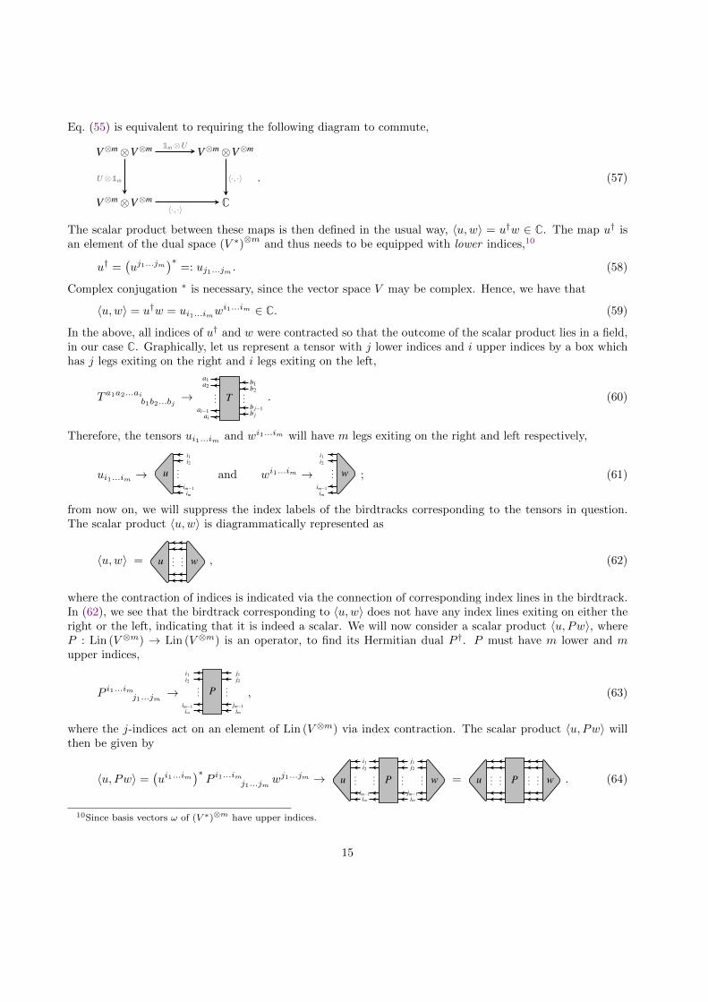
In the above, all indices of u† and w were contracted so that the outcome of the scalar product lies in a field,in our case C. Graphically, let us represent a tensor with j lower indices and i upper indices by a box whichhas j legs exiting on the right and i legs exiting on the left,
T a1a2...aib1b2...bj
→a1a2
ai−1ai
b1b2
b j−1b j
......T . (60)
Therefore, the tensors ui1...im and wi1...im will have m legs exiting on the right and left respectively,
ui1...im →...u
i1i2
im−1im
and wi1...im →i1i2
im−1im
... w ; (61)
from now on, we will suppress the index labels of the birdtracks corresponding to the tensors in question.The scalar product 〈u,w〉 is diagrammatically represented as
〈u,w〉 = ...u ... w , (62)
where the contraction of indices is indicated via the connection of corresponding index lines in the birdtrack.In (62), we see that the birdtrack corresponding to 〈u,w〉 does not have any index lines exiting on either theright or the left, indicating that it is indeed a scalar. We will now consider a scalar product 〈u, Pw〉, whereP : Lin (V ⊗m) → Lin (V ⊗m) is an operator, to find its Hermitian dual P †. P must have m lower and mupper indices,
P i1...imj1...jm →i1i2
im−1im
......P
j1j2
jm−1jm
, (63)
where the j-indices act on an element of Lin (V ⊗m) via index contraction. The scalar product 〈u, Pw〉 willthen be given by
〈u, Pw〉 =(ui1...im
)∗P i1...imj1...jm w
j1...jm → ...u
i1i2
im−1im
......P
j1j2
jm−1jm
... w = ...u ......P ... w . (64)
10Since basis vectors ω of (V ∗)⊗m have upper indices.
15

The adjoint P † of P is defined to be the object such that relation (55) holds. Thus, P † acts on the dual
space, P † : Lin(
(V ∗)⊗m)→ Lin
((V ∗)
⊗m)
, which again means that it has m upper and m lower indices,
but now the j-indices act on the element of Lin(
(V ∗)⊗m)
,
P † =(P i1...imj1...jm
)∗= P j1...jm
i1...im. (65)
It should be noted that once again, the raising and lowering of indices induces a complex conjugation ofthe tensor components, as we have already seen for u in (58).11 The same caveat applies to the associatedbirdtrack diagrams in which we have to mirror the operator about its vertical axis and reverse the directionof the arrows: i1
i2
im−1im
......P
j1j2
jm−1jm
†
=
j1j2
jm−1jm
......P†
i1i2
im−1im
. (66)
This results in all contracted index lines lining up correctly. For example,
Y 1 23
=4
3· ⇒ Y †
1 23
=4
3· (67)
=1
3
(+ − −
)=
1
3
(+ − −
).
Therefore,
〈P †u,w〉 =(uj1...jm
)∗ (P i1...imj1...jm
)∗wi1...im → ...u
j1j2
jm−1jm
......P†
i1i2
im−1im
... w = ...u ......P† ... w ; (68)
in direct correspondence with equation (64). For birdtrack operators, the Hermitean conjugate can thus begraphically formed by reflecting the birdtrack about its vertical axis and reversing the arrows, for example
reflect−−−−→ rev. arr.−−−−−→ i.e( )†
= . (69)
The mirroring of birdtracks under Hermitian conjugation immediately implies the unitarity of the primitiveinvariants (and thus that we are dealing with a unitary representation of Sm on V ⊗m): the inverse permutationof any primitive invariant ρ ∈ Sm is obtained by traversing the lines of the birdtrack corresponding to ρ inthe opposite direction [16], for example
· = =⇒ =( )−1
. (70)
However, since “traversing the lines in the opposite direction” clearly corresponds to flipping the birdtrackabout its vertical axis and reversing the direction of the arrows, we have that
ρ−1 = ρ† ∀ρ ∈ Sm ; (71)
the primitive invariants are unitary.
11The projection operators considered in this paper are real and thus remain unaffected by complex conjugation. This is nolonger true for group elements or representations.
16
These obvious Hermiticity properties of the primitive invariants make it easy to judge Hermiticity of anoperator once it is expanded in this basis set. This is no longer the case in other representations: While anymirror symmetric birdtrack represents a Hermitian operator, the converse is not true in all representations.Despite a lack of apparent mirror symmetry, the product birdtrack
(72)
is Hermitian, as can be shown by either using the simplification rules of Theorem 6 (app. C.1.1) whichallow us to recast (72) in an explicitly mirror symmetric form, or by expanding it fully in terms of primitiveinvariants.
In this paper, we will always consider birdtrack operators with lines directed from right to left (as is indicatedby the arrows on the legs). To reduce clutter, we will from now on suppress the arrows and (for example)simply write
when we mean . (73)
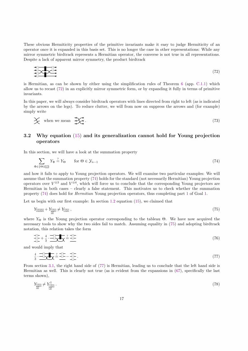
3.2 Why equation (15) and its generalization cannot hold for Young projectionoperators
In this section, we will have a look at the summation property∑Φ∈{Θ⊗n}
YΦ?= YΘ for Θ ∈ Yn−1 (74)
and how it fails to apply to Young projection operators. We will examine two particular examples: We willassume that the summation property (74) holds for the standard (not necessarily Hermitian) Young projectionoperators over V ⊗3 and V ⊗4, which will force us to conclude that the corresponding Young projectors areHermitian in both cases – clearly a false statement. This motivates us to check whether the summationproperty (74) does hold for Hermitian Young projection operators, thus completing part 1 of Goal 1.
Let us begin with our first example: In section 1.2 equation (15), we claimed that
Y 1 2 3 + Y 1 23
6= Y 1 2 , (75)
where YΘ is the Young projection operator corresponding to the tableau Θ. We have now acquired thenecessary tools to show why the two sides fail to match. Assuming equality in (75) and adopting birdtracknotation, this relation takes the form
+4
3· ?
= (76)
and would imply that
4
3· ?
= − . (77)
From section 3.1, the right hand side of (77) is Hermitian, leading us to conclude that the left hand side isHermitian as well. This is clearly not true (as is evident from the expansions in (67), specifically the lastterms shown),
Y 1 23
6= Y †1 23
. (78)
17

Thus we have arrived at a contradiction. In a similar way, it can be falsely concluded that Y 1 32
is Hermitian.
Let us now illustrate a slightly more advanced example involving an additional step which was not presentin the example for n = 3. We will explicitly discuss the case n = 4. Let us assume that equation (74) holdsfor n = 3,
Y 1 2 3 + Y 1 23
?= Y 1 2 and Y 1
23
+ Y 1 32
?= Y 1
2
(79)
and also for n = 4,
Y 1 2 3
?= Y 1 2 3 4 + Y 1 2 3
4
(80a)
Y 1 23
?= Y 1 2 4
3
+ Y 1 23 4
+ Y 1 234
(80b)
Y 1 32
?= Y 1 3 4
2
+ Y 1 32 4
+ Y 1 324
(80c)
Y 123
?= Y 1 4
23
+ Y 1234
. (80d)
Equations (80a) and (80d), if indeed valid, tell us that the operators Y 1 2 34
and Y 1 423
are Hermitian.12 To
show that the remaining operators are Hermitian, we notice that a similarity transformation with an elementρ of S4 of the form
Yi 7→ ρ†Yiρ (81)
does not change the Hermiticity of the operator Yi. Thus, for example the operator (34) · Y 1 2 34
· (34), where
(34) ∈ S4 is a transposition, is still Hermitian. It is now easy to check (via direct calculation) that13
(34) · Y 1 2 34
· (34) = Y 1 2 43
and (234) · Y 1 2 34
· (243) = Y 1 3 42
, (82)
where (243)† = (234), and similarly
(34) · Y 1 423
· (34) = Y 1 324
and (234) · Y 1 423
· (243) = Y 1 234
. (83)
We therefore conclude that also the Young projection operators Y 1 2 43
, Y 1 3 42
, Y 1 324
and Y 1 234
are Hermitian.
The remaining two operators Y 1 23 4
and Y 1 32 4
can thus be written as linear combinations of Hermitian operators,
using equations (80b) and (80c),
Y 1 23 4
=Y 1 23
−
Y 1 2 43
+ Y 1 234
(84a)
Y 1 32 4
=Y 1 32
−
Y 1 3 42
+ Y 1 324
, (84b)
12This can be concluded in the same way that we previously found that Y 1 23
is Hermitian.
13In fact, [2] defines the Young projection operator of a tableau Θ that can be obtained from Φ by reordering the entries ofΦ according to a permutation ρ as YΘ := ρ†YΦρ.
18

leading us to conclude that they are Hermitian as well. Thus, we have found that all Young projectionoperators corresponding to Young tableaux in Y4 are Hermitian – a contradiction. It should be noted that,since the Littlewood-Young projection operators over V ⊗m reduce to the Young projectors for m ≤ 4, weconclude that also the LY-operators cannot satisfy the summation property (74) (at least for m ≤ 4).
In fact, one may continue this game for one more level (to the Young projectors over V ⊗5) before the tricksgiven in the above examples seize to suffice and one has to come up with new tools.
Nonetheless, the key message to take away from this section is that the obstacle to summability is the lack ofHermiticity of the Young operators. This provides a strong hint that (74) might hold for a Hermitian versionof the Young projection operators (as was already claimed in section 1.2). In section 3.4, we show explicitlythat this is true, completing part 2 of Goal 1.
In order to be able to do so, we first need to describe how to obtain Hermitian Young projection operators.This will be the subject of the following section.
3.3 Hermitian Young projection operators: KS and beyond
3.3.1 KS construction principle
A construction principle for Hermitian Young projection operators has recently been found by Keppeler andSjodahl [1]. We will now paraphrase their construction method, see Theorem 3, as it forms a basis for provingthat the summation property eq. (74) (resp. eq. (17)) and its generalizations indeed hold for Hermitian Youngprojectors, section 3.4. We will further use Theorem 3 as a starting point for a new construction principle,which yields much more compact expressions for Hermitian Young projection operators, section 4. We willgive Keppeler and Sjodahl’s algorithm without proof; a formal proof can be found in [1].
Theorem 3 (KS Hermitian Young projectors [1]) Let Θ ∈ Yn be a Young tableau. If n ≤ 2, then theHermitian Young projection operator PΘ corresponding to the tableau Θ is given by
PΘ := YΘ. (85)
This provides a termination criterion for an iterative process that obtains PΘ from PΘ(1)via14
PΘ := PΘ(1)YΘ PΘ(1)
, (86)
once n > 2. In (86) PΘ(1)is understood to be canonically embedded in the algebra API (SU(N), V ⊗n). Thus,
PΘ is recursively obtained from the full chain of its Hermitian ancestor operators PΘ(m).
The above operators generalize properties (27) of Young projection operators to all n:
Idempotency: PΘ · PΘ = PΘ (87a)
Orthogonality: PΘ · PΦ = δΘΦPΘ (87b)
Completeness:∑
Θ∈Yn
PΘ = 1n (87c)
14In [1], eq. (86) is given as PΘ = PΘ(1)⊗ YΘ ⊗ PΘ(1)
; however, since the Pi and Yj are understood to be linear maps on
the space V ⊗n, this equation is merely a product of linear maps. The authors therefore deem the tensor-product-notationintroduced by KS unnecessarily complicated, and denote this product of linear maps as shown above.
19

As an example, consider the Young tableau
Θ =1 2 4
3 5, (88)
with ancestor tableaux15
Θ(1) =1 2 4
3, Θ(2) =
1 2
3and Θ(3) = 1 2 . (89)
When constructing the Hermitian Young projection operator PΘ according to the KS-Theorem 3, we firsthave to find PΘ(3)
, PΘ(2)and PΘ(1)
. According to the Theorem, PΘ(3)= YΘ(3)
, since Θ(3) ∈ Y2. Then,following the iterative procedure of the KS-Theorem, PΘ(2)
and PΘ(1)are given by
PΘ(2)= PΘ(3)
YΘ(2)PΘ(3)
= YΘ(3)YΘ(2)
YΘ(3)(90)
PΘ(1)= PΘ(2)
YΘ(1)PΘ(2)
= YΘ(3)YΘ(2)
YΘ(3)︸ ︷︷ ︸=PΘ(2)
YΘ(1)YΘ(3)
YΘ(2)YΘ(3)︸ ︷︷ ︸
=PΘ(2)
. (91)
Then, the desired operator PΘ is
PΘ = PΘ(1)YΘPΘ(1)
= YΘ(3)YΘ(2)
YΘ(3)YΘ(1)
YΘ(3)YΘ(2)
YΘ(3)︸ ︷︷ ︸=PΘ(1)
YΘ YΘ(3)YΘ(2)
YΘ(3)YΘ(1)
YΘ(3)YΘ(2)
YΘ(3)︸ ︷︷ ︸=PΘ(1)
. (92)
As a birdtrack, PΘ can be written as
PΘ =128
9· ︸︷︷︸YΘ(3)
︸ ︷︷ ︸YΘ(2)
︸︷︷︸YΘ(3)
︸ ︷︷ ︸YΘ(1)
︸︷︷︸YΘ(3)
︸ ︷︷ ︸YΘ(2)
︸︷︷︸YΘ(3)︸ ︷︷ ︸
PΘ(1)
︸ ︷︷ ︸YΘ
︸︷︷︸YΘ(3)
︸ ︷︷ ︸YΘ(2)
︸︷︷︸YΘ(3)
︸ ︷︷ ︸YΘ(1)
︸︷︷︸YΘ(3)
︸ ︷︷ ︸YΘ(2)
︸︷︷︸YΘ(3)︸ ︷︷ ︸
PΘ(1)
, (93)
where
128
9=(αΘ(3)
)8 (αΘ(2)
)4 (αΘ(1)
)2αΘ (94)
is the appropriate normalization constant arising from the KS-algorithm.
Let us emphasize that KS have proven that this or any other operator constructed with their algorithmis Hermitian. The operator (93) is however not symmetric under a flip about its vertical axis, and thusHermiticity is not visually obvious. An additional advantage of the construction algorithm described insection 4 is that it will necessarily yield mirror-symmetric operators, making their Hermiticity immediatelyvisible.
3.3.2 Beyond the KS construction
The results regarding Hermitian Young projection operators presented up until now are all taken from [1].We will now move beyond the established results and show that
1. the KS-operators can be simplified to yield more compact expressions, c.f. Corollary 116
15We do not have to consider the ancestor Θ(4), since Θ(3) ∈ Y2 and thus terminates the recursion (86).16While the simplification in Corollary 1 is already significant, the alternative construction given in section 4 will be even
more efficient.
20

2. the KS-operators obey the summation property (74) (resp. (17))∑Φ∈{Θ⊗n}
PΦ = PΘ ; (95)
this will be shown in section 3.4.
In [23], we found several simplification rules for birdtrack operators, some of which are summarized insection 2.3. In particular, Theorem 1 can be used to shorten the above operator (93) to
PΘ = YΘ(3)YΘ(2)
YΘ(1)YΘYΘ(1)
YΘ(2)YΘ(3)
(96)
= 8 · ︸︷︷︸YΘ(3)
︸ ︷︷ ︸YΘ(2)
︸ ︷︷ ︸YΘ(1)
︸ ︷︷ ︸YΘ
︸ ︷︷ ︸YΘ(1)
︸ ︷︷ ︸YΘ(2)
︸︷︷︸YΘ(3)
, (97)
where(αΘ(3)
αΘ(2)αΘ(1)
)2αΘ = 8. The above expression for PΘ is clearly considerably shorter than the
expression given in (93). In fact, Theorem 1 allows us to systematically shorten the KS-projection operators,exposing a new, much simpler general form:
Corollary 1 (staircase form of Hermitian Young projectors) Let Θ ∈ Yn be a Young tableau. Then,the corresponding Hermitian Young projection operator PΘ is given by
PΘ = YΘ(n−2)YΘ(n−3)
YΘ(n−4). . . YΘ(2)
YΘ(1)YΘ YΘ(1)
YΘ(2). . . YΘ(n−4)
YΘ(n−3)YΘ(n−2)
. (98)
This result simply follows from a repeated application of Theorem 1, where we notice that Θ(n−2) ∈ Y2
necessarily.
Even though this simplification is already quite substantial, it is by no means the simplest form achievable.We will present a new construction principle in section 4, creating even more compact and thus easier usableHermitian Young projection operators. The proof of this construction will however make use of the KS-Theorem 3, see app. C.
3.4 Spanning subspaces with Hermitian operators
We are finally in a position to show that∑Φ∈{Θ⊗n}
PΦ = PΘ (99)
holds for every Θ ∈ Yn−1 if the PΞ are the Hermitian operators introduced previously. In section 1.2, wegave the particular example
P 1 2 3 + P 1 23
= P 1 2 (100)
which holds for the Hermitian Young operators PΞ but fails to hold for their Young operator counterparts.
To prove (99) in general, we first need to show that a projection operator PΘ projects onto a subspace of theimage of an operator PΘ(m)
, where Θ(m) is an ancestor tableau of Θ. In particular, this will mean that theimage of an operator PΘ is a subset of the image of its parent operator PΘ(1)
.
21

Lemma 1 (Subspaces corresponding to Hermitian Young projection operators are nested) LetΘ ∈ Yn be a Young tableau and let Θ(m) be its ancestor tableau, with m < n. Furthermore, let PΘ and PΘ(m)
be the Hermitian Young projection operators corresponding to these tableaux. Then, the image of PΘ liesentirely in the image of PΘ(m)
,
PΘPΘ(m)= PΘ = PΘ(m)
PΘ . (101)
An immediate consequence of this Lemma is that a Hermitian Young projection operator PΘ commutes withits ancestor operator PΘ(m)
. In appendix B, we first exemplify that Young projectors do not necessarily obeythe analgous image inclusion properties YΘYΘ(m)
= YΘ and/or YΘ(m)YΘ = YΘ. We prove that where the
image inclusion fails to hold the associated commutator [YΘ(m), YΘ] does not vanish.
Image inclusion will play an integral part in the proof of eq. (99) and thus highlights where the proof wouldbreak down for the (not necessarily Hermitian) Young projectors.
Before we give the proof of Lemma 1, We wish to draw attention to how this proof makes use of some of thesimplification rules given in section 2.3, as this will be mirrored in the proofs of the main Theorems given inappendix C.
Proof of Lemma 1: To prove the inclusion of the subspaces, it suffices to show that the product of theoperators satisfies eq. (101) (c.f. eq. (40)). What this relation implies is that if we first act the productPΘ(m)
PΘ (or equivalently PΘPΘ(m)) on an object x, we obtain the same outcome as if we only act PΘ on
x. Hence, PΘ must correspond to a smaller subspace than PΘ(m), and this subspace must completely be
contained in the subspace corresponding to PΘ(m). From the shortened KS construction, Corollary 1, the
Hermitian Young projection operators PΘ and PΘ(m)are given by
PΘ = YΘ(n−2)YΘ(n−3)
. . . YΘ(m+1)YΘ(m)
. . . YΘ(1)YΘ YΘ(1)
. . . YΘ(m)YΘ(m+1)
. . . YΘ(n−3)YΘ(n−2)
(102)
PΘ(m)= YΘ(n−2)
YΘ(n−3). . . YΘ(m+1)
YΘ(m)YΘ(m+1)
. . . YΘ(n−2)YΘ(n−2)
. (103)
When forming the product PΘPΘ(m), we see a lot of cancellation of wedged ancestor operators due to Theo-
rem 1,
PΘ · PΘ(m)= YΘ(n−2)
. . . YΘ(m). . . YΘ(1)
YΘ YΘ(1). . . YΘ(m)
. . . YΘ(n−2)· YΘ(n−2)
. . . YΘ(m)︸ ︷︷ ︸= YΘ(m)
. . . YΘ(n−2)
= YΘ(n−2). . . YΘ(m)
. . . YΘ(1)YΘ YΘ(1)
. . . YΘ(m). . . YΘ(n−2)
. (104)
The above can easily be identified to be the operator PΘ, yielding the first equality PΘPΘ(m)= PΘ. The
second equality can similarly be shown, leading to the desired result.
Let us now prove the summation property (99) for Hermitian Young projection operators: Recall the com-pleteness relation of Hermitian Young projection operators, eq. (87c),∑
Θ∈Yn−1
PΘ = idn−1, (105)
where idk is the identity operator on the space V ⊗k. Equation (105) can be canonically embedded into thespace V ⊗n as was discussed in section 2.2.2. In order to make the embedding of the operator PΘ explicit, we
22
will – for this section only – make the identity operator on the last factor explicitly visible in the birdtrackspirit and denote the embedded operator by the symbol PΘ.17 The embedded equation (105) thus is∑
Θ∈Yn−1
PΘ = idn. (106)
Even though (106) is a decomposition of unity, a finer decomposition of idn (also using only orthogonalobjects) is obtained with Hermitian Young projection operators corresponding to Young tableaux in Yn,∑
Φ∈Yn
PΦ = idn. (107)
Since clearly Yn is the union of all the sets {Θ⊗ n }, for all Θ ∈ Yn−1, the sum (107) can be split into
∑Φ∈Yn
PΦ =∑
Θ∈Yn−1
∑Ψ∈{Θ⊗n}
PΨ
= idn. (108)
Since both (106) and (108) are a decomposition of idn, they must be equal to each other, yielding
∑Θ∈Yn−1
PΘ =∑
Θ∈Yn−1
∑Ψ∈{Θ⊗n}
PΨ
. (109)
Let us now multiply the above equation with a particular operator PΘ′ on V ⊗n, where Θ′ is a particulartableau in Yn−1. Due to the orthogonality property (eq. (87b), Theorem 3) and the inclusion property(eq. (101), Lemma 1) of Hermitian Young projectors,18 it follows that
∑Θ∈Yn−1
δΘΘ′PΘ =∑
Θ∈Yn−1
δΘΘ′
∑Ψ∈{Θ⊗n}
PΨ
(110)
PΘ′ =∑
Ψ∈{Θ′⊗n}
PΨ , (111)
yielding the desired equation (99). This concludes part 2 of Goal 1.
Since the Hermitian operators sum up to their Hermitian parent operators (eq. (111)), and these in turn sumto their Hermitian parent operators, the summation property necessarily holds over multiple generations.This statement also follows straight from Lemma 1, which states that the image of a Hermitian Youngprojection operator PΘ is contained in the image of its Hermitian ancestor operator PΘ(m)
, where m can beany positive integer. Therefore, if YΘ,n := {Θ ⊗ m ⊗ · · · ⊗ n } is the subset of Yn containing all tableauxthat have Θ ∈ Ym−1 as their ancestor, then∑
Φ∈YΘ,n
PΦ = PΘ , (112)
17In birdtrack notation, the canonically embedded operator PΘ will be PΘ with an extra index line on the bottom, makingthe notation PΘ intuitive.
18This is where the proof would break down for the standard Young projection operators even for n ≤ 4, where they explicitlydo not satisfy the image inclusion property (101), c.f. appendix B.
23

confirming eq. (18). For example, if Θ = 1 2 3 , then PΘ can be written as a sum of the following HermitianYoung projection operators corresponding to tableaux in Y5,
P 1 2 3 4 5 + P 1 2 3 45
+ P 1 2 3 54
+ P 1 2 34 5
+ P 1 2 345︸ ︷︷ ︸∑
Φ∈YΘ,5PΦ
= P 1 2 3︸ ︷︷ ︸PΘ
. (113)
This concludes the last part (part 3) of the first Goal of this paper.
Figure 1 shows all Hermitian Young projectors corresponding to Young tableaux in Yn up to and includingn = 4. The arrows in this figure indicate which operators sum to which ancestor operators. The summationproperty of Hermitian Young projectors was not mentioned in [16, fig. 9.1] where a virtually identical figurecan be found.
4 An algorithm to construct compact expressions of HermitianYoung projection operators
We will now come to Goal 2 of this paper and provide a construction principle that allows us to directly arriveat compact expressions for Hermitian Young projection operators (see Theorem 5 below). This constructionyields much shorter expressions than the previously encountered KS algorithm (Theorem 3), or even theshortened version of Theorem 1, as is exemplified in Fig. 2.
4.1 Lexically ordered Young tableaux
It turns out that the ordering of the numbers within the Young tableau plays a vital role in our algorithm.Thus, we will first establish what we mean by the lexical order of a Young tableau. To do so, we will introducecolumn- and row-words:19
Definition 2 (column- and row-words & lexical ordering) Let Θ ∈ Yn be a Young tableau. We definethe column-word of Θ, CΘ, to be the column vector whose entries are the entries of Θ as read column-wisefrom left to right. Similarly, the row-word of Θ, RΘ, is defined to be the row vector whose entries are thoseof Θ read row-wise from top to bottom.
We will call a tableau Θ lexically ordered, if either CΘ or RΘ or both are in lexical order. In particular, wesay that Θ is column-ordered (resp. row-ordered), if CΘ (resp. RΘ) is in lexical order.
For example, the tableau
Φ :=
1 5 7 9
2 6 8
3
4
(114)
has a column-word
CΦ = (1, 2, 3, 4, 5, 6, 7, 8, 9)t, (115)
19It should be noted that Definition 2 of the row-word is different to the definition given in the standard literature suchas [13, 24]: there, the row word is read from bottom to top rather than from top to bottom. However, for the purposes of thispaper, Definition 2 is more useful than the standard definition.
24

P 1 =
P 1 2 =
P 12=
P 1 2 3 =
P 1 23
=
43
P 1 32
=
43
P 123
=
P 1 2 3 4 =
P 1 2 34
=
32
P 1 2 43
=
2
P 1 23 4
=
43
P 1 234
=
32
P 1 3 42
=
32
P 1 32 4
=
43
P 1 324
=
2
P 1 423
=
32
P 1234
=
d = N
d =N(N+1)
2
d =N(N−1)
2
d =N(N+1)(N+2)
6
d =N(N2−1)
3
d =N(N−1)(N−2)
6
d =N(N+1)(N+2)(N+3)
24
d =N(N+2)(N2−1)
8
d =N2(N2−1)
12
d =N(N−2)(N2−1)
8
d =N(N−1)(N−2)(N−3)
24
Figure 1: Hierarchy of Young tableaux and the associated nested Hermitian Young projector decompositions(in the sense of embeddings into API
(SU(N), V ⊗4
)): Projection operators that are contained in a gray
box correspond to equivalent irreducible representations of SU(N), as their corresponding Young tableauxhave the same shape [2, 16]. The dimension of the irreducible representation corresponding to a (set of)operators(s) is given on the left [16, fig. 9.1]. The arrows indicate which operators sum to which ancestor –this summation property of Hermitian Young projection operators was not observed by [16].
25

and a row-word
RΦ = (1, 5, 7, 9, 2, 6, 8, 3, 4). (116)
From this, we see that Φ in (114) is lexically ordered. In particular, it is column-ordered (but not row-ordered).
In Theorem 4 we will describe a construction principle for the Hermitian Young projection operators corre-sponding to lexically ordered tableaux. This will form a starting point for the general construction principleof the Hermitian Young projectors given in section 4.2, as is evident from their proofs in appendix C. It isclear that Keppeler and Sjodahl had noticed that the projectors associated with ordered tableaux are special:In the appendix of [1] they discuss two examples of Hermitian Young projection operators (which happen tocorrespond to lexically ordered tableaux) constructed according to the KS-Theorem, and argue that theseoperators can be simplified quite drastically. The procedure leads eventually to the same expressions thatemerge directly from Theorem 4. However, Keppeler and Sjodahl do not establish the connection to thelexical order of the Young tableau and do not even hint at a general construction principle.
Theorem 4 (lexical Hermitian Young projectors) Let Θ ∈ Yn be row-ordered. Then, the correspond-ing Hermitian Young projection operator PΘ is given by
PΘ = αΘ · YΘY†Θ. (117a)
On the other hand, if Θ ∈ Yn is a column-ordered tableau, then the corresponding Hermitian Young projectionoperator PΘ is given by
PΘ = αΘ · Y †ΘYΘ. (117b)
The proof of this Theorem is deferred to Appendix C.1. It is directly evident from eqns. (117a) and (117b)that PΘ is Hermitian in both cases. Since Hermitian conjugation in birdtrack notation amounts to reflectionabout a vertical axis, the formulae also guarantee that Hermiticity is directly visible as a reflection symmetryof the associated birdtrack diagrams.
As an example, consider the Young tableau
Θ =1 2
3(118)
which has a lexically ordered row-word RΘ = (1, 2, 3). The associated Hermitian Young projection operatorPΘ according to the Lexical-Theorem 4 is given by
PΘ =4
3︸︷︷︸αΘ
· ︸ ︷︷ ︸YΘ
︸ ︷︷ ︸Y †Θ
=4
3· ︸ ︷︷ ︸
=:PΘ
. (119)
The Hermiticity of this operator is prominently visible in its mirror symmetry.
4.2 Young tableaux with partial lexical order
We will now give a construction principle for compact expressions of Hermitian Young projection operatorscorresponding to general, not necessarily lexically ordered, tableaux. The goal is to use what partial orderthere is to a diagram to obtain an optimized iterative procedure. As a first step we need to be able to quantifyhow “un-ordered” a Young tableau is; we define a Measure Of Lexical Disorder :
26

Definition 3 (measure of lexical disorder (MOLD)) Let Θ ∈ Yn be a Young tableau. We define itsMeasure Of Lexical Disorder (MOLD) to be the smallest natural number M(Θ) ∈ N such that
Θ(M(Θ)) = πM(Θ) (Θ) (120)
is a lexically ordered tableau. (Recall from Definition 1 that πM(Θ) refers to M(Θ) consecutive applicationsof the parent map π to the tableau Θ.)
We note that the MOLD of a Young tableau is a well-defined quantity, since one will always eventually arriveat a lexically ordered tableau, as, for example, all tableaux in Y3 are lexically ordered. This then impliesthat the MOLD of a tableau Θ ∈ Yn has an upper bound,
M(Θ) ≤ n− 3, (121)
making it a well-defined quantity. As an example, consider the tableau
Φ :=1 2 4
3 5. (122)
The MOLD of the above tableau is M(Φ) = 2, since two applications of the parent map generate a lexicallyordered tableau, but just one application of π on Φ would not be sufficient,
1 2 4
3 5︸ ︷︷ ︸Φ
π−−→ 1 2 4
3︸ ︷︷ ︸Φ(1)
π−−→ 1 2
3︸ ︷︷ ︸Φ(2)
. (123)
We will now give the main Theorem of this section, the construction principle of Hermitian Young projectionoperators corresponding to Young tableaux Θ, using the MOLD of the latter. To do so, we distinguish fourcases; the reason why they have to be dealt with separately is given in the analysis following the Theorem,section 4.2.1.
Theorem 5 (MOLD operators) Consider a Young tableau Θ ∈ Yn with MOLD M(Θ) = m. Further-more, suppose that Θ(m) has a lexically ordered row-word. Then, the Hermitian Young projection operatorcorresponding to Θ, PΘ, is, for m even,
PΘ = βΘ ·SΘ(m)AΘ(m−1)
SΘ(m−2). . . SΘ(2)
AΘ(1)YΘY
†Θ AΘ(1)
SΘ(2). . . SΘ(m−2)
AΘ(m−1)SΘ(m)
, (124a)
and, for m odd,
PΘ = βΘ ·SΘ(m)AΘ(m−1)
SΘ(m−2). . . AΘ(2)
SΘ(1)Y †ΘYΘ SΘ(1)
AΘ(2). . . SΘ(m−2)
AΘ(m−1)SΘ(m)
. (124b)
Similarly, if Θ(m) has a lexically ordered column-word, PΘ is, for m even,
PΘ = βΘ ·AΘ(m)SΘ(m−1)
AΘ(m−2). . . AΘ(2)
SΘ(1)Y †ΘYΘ SΘ(1)
AΘ(2). . . AΘ(m−2)
SΘ(m−1)AΘ(m)
, (124c)
and, for m odd,
PΘ = βΘ ·AΘ(m)SΘ(m−1)
AΘ(m−2). . . SΘ(2)
AΘ(1)YΘY
†Θ AΘ(1)
SΘ(2). . . AΘ(m−2)
SΘ(m−1)AΘ(m)
. (124d)
In the above, all symmetrizers and antisymmetrizers are understood to be canonically embedded into V ⊗n;βΘ is a non-zero constant chosen such that PΘ is idempotent.
27

The formal proof of this Theorem can be found in Appendix C.2. A comparative example of a HermitianYoung projection operator constructed using MOLD and KS is given is section 4.3, Fig 2.
It should be noted that we have not provided an explicit expression for the constant βΘ in Theorem 5.This normalization-constant however can easily be found for specific operators by direct calculation since theMOLD-operators are very much suited for automated calculations on a computer, as is described in section 4.3.We would like to draw the reader’s attention to the fact that the symmetrizers and antisymmetrizers in allfour expressions of Theorem 5 strictly alternate, including those inside the Young projectors.
As an example, consider the Young tableau
Θ :=1 2 4
3 5. (125)
This tableau has MOLD 2 (i.e. even MOLD), and Θ(2) has a lexically ordered row-word. Thus, we have toconstruct the Hermitian Young projection operator PΘ corresponding to Θ according to equation (124a). PΘ
is therefore given by
PΘ = βΘ · SΘ(2)AΘ(1)
SΘ AΘ SΘ AΘ(1)SΘ(2)
= βΘ · ︸︷︷︸SΘ(2)
︸ ︷︷ ︸AΘ(1)
︸ ︷︷ ︸SΘ
︸ ︷︷ ︸AΘ
︸ ︷︷ ︸SΘ
︸ ︷︷ ︸AΘ(1)
︸︷︷︸SΘ(2)
= βΘ · . (126)
A direct calculation in Mathematica reveals that βΘ!= 4 for PΘ to be idempotent.
4.2.1 A Short Analysis of the MOLD-Theorem 5
We now pause for a moment to look at the four cases presented in Theorem 5 in more detail and emphasizetheir differences. We hope to convey an intuitive feel as to why the corresponding operators are constructedthe way they are.
First, let us look at the first two operators (124a) and (124b). Both these operators PΘ have a symmetrizeron the outside, namely SΘ(m)
, opposed to the operators (124c) and (124d) which have an antisymmetrizeron the outside. This stems from the iterative construction of Hermitian Young projection operators given bythe KS-Theorem 3: By the Lexical-Theorem 4 we know that PΘ(m)
is given by
PΘ(m)= αΘ · YΘ(m)
Y †Θ(m)= αΘ · SΘ(m)
AΘ(m)SΘ(m)
, (127)
since PΘ(m)is assumed to correspond to a row-ordered Young tableau. When we thus construct PΘ recursively
according to KS, [1], we find that
PΘ = PΘ(m). . . YΘ . . . PΘ(m)
∝ SΘ(m)AΘ(m)
SΘ(m). . . YΘ . . .SΘ(m)
AΘ(m)SΘ(m)
. (128)
Thus, we expect there to be symmetrizers on the outside of the operators PΘ in expressions (124a) and(124b). Following a similar logic, we expect there to be antisymmetrizers on the outside of operators (124c)and (124d).
Lastly, we discuss the importance of the distinction between even and odd m in the MOLD-Theorem 5. Inthe construction of all PΘ in the Theorem, we find that they consist of products of alternating symmetrizers
28

and antisymmetrizers to more and more recent generations of Θ as we move further to the center of PΘ. If theoperator PΘ thus starts with S(m) on the outside, as it does in equations (124a) and (124b), and the producthas alternating sets of symmetrizers and antisymmetrizers each going up one generation, then the parity ofm will decide whether the set corresponding to the tableau Θ(1) in the product PΘ is a set of symmetrizersor antisymmetrizers. Thus, the central three sets of symmetrizers and antisymmetrizers in the product PΘ
will then either be
AΘ SΘ AΘ = Y †ΘYΘ or SΘ AΘ SΘ = YΘY†Θ, (129)
dependent on the nature of the sets corresponding to Θ(1), but keeping the alternating structure of sym-metrizers and antisymmetrizers.
The fact that the central sets of PΘ in all four equations of the above Theorem 5 are either product of(129) opposed to simply YΘ or Y †Θ can be attributed to the fact the PΘ is Hermitian and we would like itsHermiticity to be visually explicit.
4.3 The advantage of using MOLD
The practical advantages of our construction opposed to the KS-Theorem 3 are striking. To illustrate this wereturn to the same example used in [23] to demonstrate the effectiveness of the simplification rules derivedthere. The Young tableau
Φ :=
1 2 4 7
3 6
5 8
9
(130)
leads to an expression of the corresponding KS-projector with 127 symmetrizer- and antisymmetrizer-setswhich reduce to an object with only 13 such sets after applying the cancellation and propagation rules of [23].
Both construction principles (KS and MOLD) are iterative in the sense that they both require knowledgeabout the ancestor tableaux of a tableau Θ ∈ Yn. For the construction of KS as it was originally describedin [1], one needs all ancestor operators of Θ up until Θ(n−2), while the MOLD construction merely uses theancestor tableaux up until ΘM(Θ), which is at most Θ(n−3) according to (121). This one tableau differencedoes not seem excessive at first glance, but one should keep in mind that the difference is at least onetableau, often more. However the bulk of the computing power used to generate PKSΦ comes from the factthat, in addition to the ancestor tableaux of Θ, one further requires information about the explicit form of theancestor Hermitian Young projectors PΘ all the way up to PΘ(2)
, which have to be calculated separately. TheMOLD-construction merely uses the Young sets of symmetrizers or antisymmetrizers (S and A respectively)of the ancestor tableaux of Θ up to ΘM(Θ), which can be immediately read off the tableaux and thus needsminimal computing power.
Using the MOLD-Theorem 5, one arrives at the shorter version directly, after a considerably shorter recursivepath and without the need for additional simplifications. One bypasses a long repetitive list of steps altogether!The 127/13 length ratio between PKS
Φ and PMOLDΦ
20 is strikingly apparent in Fig. 2. This makes the MOLDalgorithm a lot more practical to work with analytically. The algorithm really comes into its own when used
20It is important to note that PKSΦ and PMOLDΦ both differ from PΦ by a constant, but this constant will depend on the
construction principle used to find PΦ. In that sense,
βKSΦ · PKSΦ = PΦ = βMOLDΦ · PMOLD
Φ (131)
but βKSΦ 6= βMOLD
Φ in general.
29

Figure 2: For a size comparison, this figure shows PKSΦ (top) and PMOLD
Φ (bottom) for the tableau Φ asdefined in (130) using two different constructions: The top operator was constructed using the KS-algorithm,while the bottom operator was constructed using MOLD. Both operators and the associated graphics weregenerated in Mathematica.
in symbolic algebra programs: the MOLD construction allows us to efficiently create projection operatorsfor considerably larger Young tableaux than the iterative KS equivalent. In particular, for the examplein Figure 2, the fact that the MOLD algorithm simply avoids a long series of steps makes it over 18600times faster than its KS counterpart: It generates its result in approximately 0.0038 seconds, while KS takesapproximately 71 seconds (not even taking into account the cost of the simplification steps to arrive at thefinal result) on a modern laptop.
Unlike PKSΘ , PMOLD
Θ is obviously and visibly Hermitian by construction.21 Given that birdtracks are meantto be a tool that makes dealing with these operators visually clear, this is an obvious advantage.
We have given a construction principle for compact expressions of Hermitian Young projection operators, theMOLD-operators, in section 4.2, and we have now seen that the MOLD-operators are indeed more useful forpractical calculations. We have thus achieved Goal 2 of this paper.
5 Conclusion & outlook
The representation theory of SU(N) is an old theory with many successful applications in physics. Yet someof the tools remain awkward and only applicable in specific situations, like the general theory of angularmomentum or the construction of Young projection operators that lack Hermiticity. Newer tools like thebirdtrack formalism remain only partially connected with these time honored results. We have a very specificinterest in applications to QCD in the JIMWLK context, in jet physics, in energy loss and generalized partondistributions, so we have aimed at creating a set of tools that we know will aid in these applications and, inthe process have pointed out where the existing tools fall short of our needs.
1. We have found that projection operators built on Young tableaux are uniquely suited to calculationsthat keep N as a parameter.
To simply list the irreducible multiplets in V ⊗m, Young’s procedure forms descendant tableaux ofthose representing the irreducibles contained in V ⊗(m−1), portraying an iterative procedure of “addinga particle” in each step.
To parallel this in terms of projection operators and the associated subspaces (i.e. to implement eq. (112)which represents the general case of the summation relations collected in Fig. 1) – as one needs to doto actually perform calculations in physics applications – we have established that one needs Hermitianversions of these projection operators as those constructed earlier by Keppeler and Sjodahl [1]. Thissets the backdrop for the remaining developments.
21PKSΘ do not exhibit their Hermiticity directly since the center-piece of the KS operator is the Young projection operatorYΘ, which is inherently non-Hermitian. We need to rely on the proof given in [1] to be assured of their Hermiticity.
30

2. Having motivated the necessity for Hermitian Young projection operators, we are faced with the factthat the KS algorithm quickly becomes unwieldy – the iterative procedures are computationally expen-sive and produce long expressions (Fig. 2). We have earlier presented simplification rules [23] to distillthese down to more compact expressions, but that does not alleviate the computational cost.
To address this issue, we have provided a new algorithm based on the Measure Of Lexical Disorder(MOLD) of a tableau in sec. 4.2 that drastically reduces the calculational footprint of the procedurecompared to the KS method. It should be noted that the normalized operators constructed using theMOLD algorithm are equal to the KS-operators (as is evident from the proof given in appendix C) andthus inherit all properties of the KS-operators: idempotency, mutual orthogonality and completenessfor all values of m.
The MOLD algorithm almost completely incorporates the simplifications of [23] at vastly reducedcalculational cost (only isolated cases of MOLD-operators still allow for further simplification with thetools presented in [23]). All the algorithms are eminently suited for implementation in symbolic algebraprograms: all our explorations and examples have been generated in Mathematica.
In particular, the operators shown in Fig. 2 were generated in Mathematica: the operator on the topwas constructed using the KS-Theorem, while the operator on the bottom resulted from the MOLD-construction. The automated calculation was significantly improved with the MOLD-algorithm, as theMOLD-operator in Fig. 2 was obtained approximately 18600 times faster than the KS-equivalent on amodern laptop – an improvement of 4 orders of magnitude.
Our own list of applications for the tools and insights presented in this paper are QCD centric: Global singletstate projections of Wilson-line operators that appear in a myriad of applications due to factorization ofhard and soft contributions help analyzing the physics content in all of them; this will be explored furtherin [22]. We hope that our presentation is suitable to unify perspectives provided by the various approachesto representation theory of SU(N) and that the results prove useful beyond these immediate applications.
Acknowledgements: H.W. is supported by South Africa’s National Research Foundation under CPRRgrant nr 90509. J.A-Z. was supported (in sequence) by the postgraduate funding office of the University ofCape Town (2014), the National Research Foundation (2015) and the Science Faculty PhD Fellowship of theUniversity of Cape Town (2016).
A Littlewood-Young projection operators
For completeness, this appendix summarizes the construction principle of generalized Young projection op-erators due to Littlewood [18, sec. 5.3], which corrects for the failure of Young projection operators over V ⊗n
to be orthogonal or complete beyond n = 4. We shall call these the Littlewood-Young (LY) projectors anddenote them by L.
Before we give the construction principle of the LY-projectors, let us have a closer look at products of Youngprojection operators and criteria which make these products orthogonal. Consider two Young tableaux Θand Φ in Yn, then the product of their corresponding Young projection operators is given by
YΘYΦ = αΘαΦ · SΘAΘSΦAΦ . (132)
Clearly, if the product AΘSΦ vanishes, then so does the product of the Young projectors, but if AΘSΦ 6= 0,
31

we have to conclude that YΘYΦ 6= 0,
YΘYΦ = αΘαΦ · SΘ AΘ SΦ AΦ =⇒ YΘYΦ 6= 0 .6= 0 6= 0
6= 0
(133)
For AΘSΦ to vanish, we merely require a particular antisymmetrizer Ai ∈ AΘ two have more than one legin common with a symmetrizer Sj ∈ SΦ.
If the tableaux Θ and Φ have different shapes, then this is trivially given since there must exist at least onepair of boxes ( k , l ) that appear in the same column in Θ and in the same row in Φ and vice versa, suchthat [18, sec. 5.3, Thm. III]
AΘSΦ = 0 = AΦSΘ where Θ and Φ have different shapes . (134)
If the two tableaux Θ and Φ have the same shape, one must work harder to see where this criterion appliesto force AΘSΦ = 0. To see when a pair of boxes ( k , l ) appears in the same column in Θ and in the samerow in Φ for tableaux of the same shape, we need to introduce an order relation between tableaux of thesame shape using their row-words (c.f. Definition 2):
Definition 4 (order relation amongst tableaux of the same shape) Let Θ and Φ be two Youngtableaux and let θij be the entry in the ith row and jth column of Θ, and similarly for φij. Their correspondingrow-words are given by RΘ = (θ11, θ12, . . . , θ21, . . .) and RΦ = (φ11, φ12, . . . , φ21, . . .) respectively. We saythat Θ precedes Φ and write Θ ≺ Φ if θij < φij for the leftmost ij where θij ∈ RΘ and φij ∈ RΦ differ.22
For example, the Young tableaux of shape can be ordered as
1 2 3
4 5︸ ︷︷ ︸RΘ=(1,2,3,4,5)
≺ 1 2 4
3 5︸ ︷︷ ︸RΘ=(1,2,4,3,5)
≺ 1 2 5
3 4︸ ︷︷ ︸RΘ=(1,2,5,3,4)
≺ 1 3 4
2 5︸ ︷︷ ︸RΘ=(1,3,4,2,5)
≺ 1 3 5
2 4︸ ︷︷ ︸RΘ=(1,3,5,2,4)
. (135)
It turns out that this order relation defines exactly when a pair of boxes ( k , l ) appearing in the samecolumn of a tableau Θ appear in the same row of a tableau Φ forcing the product AΘSΦ to vanish [18,sec. 5.3, Thm. V]. We repeat the proof given by [18]: Let Θ and Φ be two Young tableaux of the same shapeand let Θ ≺ Φ. Then, the first entry θij ∈ RΘ distinct from φij ∈ RΦ satisfies θij < φij . Thus, the entryφkl ∈ RΦ such that θij = φkl must appear in a row later than i, but, by definition of Young tableaux, mustbe in a column before j,
θij = φkl with l < j and k > i . (136)
Since l < j, the entries θil and φil must be equal (we assumed that the entries θij and φij were the firstdistinct entries appearing in the respective row-words), θil = φil. Thus, the pair of entries (θij = φkl, θil = φil)appears in the same row in Θ (the ith row) and in the same column in Φ (the lth column), yielding AΦSΘ = 0.Thus, we can say that
YΦYΘ = 0 if Θ ≺ Φ . (137)
It should be noted that the reverse not necessarily holds, that is
Θ ≺ Φ 6=⇒ YΘYΦ = 0 . (138)
22In words, we order a set of tableaux according to the relative lexical order of their associated row words. This concept isnot to be confused with the lexical order within a tableau introduced in Defintion 2.
32

Littlewood uses this one-sided orthogonality of Young projection operators to create mutually orthogonalones:
Let {Θ1,Θ2, . . .Θk} be the set of all Young tableaux in Yn with a particular shape and let them be orderedsuch that Θi ≺ Θj whenever i < j. From eq. (137), we have that
YΘjYΘi = 0 whenever i < j . (139)
The Littlewood-Young projection operators LΘi corresponding to the tableaux Θi ∈ {Θ1,Θ2, . . .Θk} ⊂ Ynare defined as
LΘ1 = YΘ1
LΘ2 = (1− LΘ1)YΘ2
...
LΘk = (1− LΘ1− LΘ2
− . . .− LΘk−1)YΘk . (140)
It should be noticed that the LY-operators corresponding to tableaux in Yn for n ≤ 4 reduce to the Youngprojectors, as in these instances the Young projectors are mutually orthogonal. Even for n > 5, many LY-projectors reduce to the regular Young projectors, or at least simplify drastically since most of the Youngprojectors remain orthogonal even for large n. As an example, at n = 5 the only two Littlewood-Youngprojection operators that differ from their Young counterpart are given by
L 1 3 52 4
=
(1− Y 1 2 3
4 5
)Y 1 3 5
2 4
and L 1 42 53
=
1− Y 1 23 45
Y 1 42 53
. (141)
The LY-operators constructed according to (140) are orthogonal for all values of n: If two operators LΘ
and LΦ correspond to tableaux of different shapes, then LΘ and LΦ are orthogonal since their respectiveconstituent Young projection operators are orthogonal. If LΘi and LΘj correspond to tableaux of the sameshape with Θi ≺ Θj (i < j), then
LΘjLΘi = 0 from eq. (139) (142)
To show the reverse (LΘiLΘj = 0), it is highly advantageous to note that LΘj as given in (140) can be recastas
LΘj = (1− YΘ1)(1− YΘ2) · · · (1− YΘj−1)YΘj . (143)
This can be shown by induction: For j = 1, 2 eq. (143) trivially holds, we therefore go through the case j = 3explicitly:
LΘ3 =(
1− YΘ1︸︷︷︸=LΘ1
− (1− YΘ1)YΘ2︸ ︷︷ ︸=LΘ2
)YΘ3 =
((1−YΘ1)− (1−YΘ1)YΘ2
)YΘ3 = (1−YΘ1)(1−YΘ2)YΘ3 . (144)
33

Suppose eq. (143) holds for all LΘk up some integer k = j − 1. Then, by eq. (140), LΘj is given by
LΘj =(
1− YΘ1︸ ︷︷ ︸=(1−YΘ1 )
−(1− YΘ1)YΘ2
− . . .− (1− YΘ1)(1− YΘ2
) · · · (1− YΘj−2)YΘj−1
)YΘj
= (1− YΘ1)(
1− YΘ2︸ ︷︷ ︸=(1−YΘ2
)
−(1− YΘ2)YΘ3 − . . .− (1− YΘ2) · · · (1− YΘj−2)YΘj−1
)YΘj
= (1− YΘ1)(1− YΘ2
)(
1− YΘ3︸ ︷︷ ︸=(1−YΘ3
)
−(1− YΘ3)YΘ4
− . . .− (1− YΘ3) · · · (1− YΘj−2
)YΘj−1
)YΘj
...
= (1− YΘ1)(1− YΘ2) · · · (1− YΘj−1)YΘj , (145)
confirming eq. (143).
Let
MΘi−1 := (1− YΘ1)(1− YΘ2) · · · (1− YΘi−1) (146)
such that LΘi = MΘi−1YΘi . From eq. (139) is is clear that
YΘk(1− YΘl) = YΘk − 0 = YΘk for every l < k . (147)
Thus, if i < j we have that
LΘi · LΘj = MΘi−1YΘi︸ ︷︷ ︸=LΘi
· (1− YΘ1) · · · (1− YΘi) · · · (1− YΘj−1
)YΘj︸ ︷︷ ︸=LΘj
= MΘi−1YΘi(1− YΘi)︸ ︷︷ ︸=YΘi
−Y 2Θi
=0
· · · (1− YΘj−1)YΘj
= 0 , (148)
where we used the fact that Young projectors are idempotent (Y 2Θi
= YΘi). Thus, LΘi and LΘj are orthogonaleven if i < j.
We notice that the LΘ remain idempotent just like their Young counterparts,
LΘi ·LΘi = LΘi (1− LΘ1 − LΘ2 − . . .− LΘi−1)YΘ1︸ ︷︷ ︸=LΘi
= (LΘi − 0− 0− . . .− 0)YΘ1 = LΘiYΘi = LΘi . (149)
Putting everything together, we can conclude that
LΘLΦ = δΘΦLΦ for all Θ,Φ ∈ Yn for all values of n , (150)
confirming eqns. (6a) and (6b).
Since the LY-operators are mutually orthogonal (eq. (150)), they can be simultaneously diagonalised andhave mutually orthogonal images. Since they are idempotent their trace provides the dimension of theirimage:
Tr (LΘ) = dim(Θ) . (151)
34

Thus, if we can show that the dimensions of the subspaces corresponding to the LΘ sum up to the dimensionof the whole space dim(V ⊗n) = Nn, it must hold that the orthogonal operators LΘ sum up to the identityon V ⊗n. To show this, we notice that LΘ has the same trace as its counterpart YΘ: Using the cyclic propertyof the trace, we have
Tr (LΘi) = Tr((1− LΘ1
− LΘ2− . . .− LΘi−1
)YΘi
)= Tr
(YΘi(1− LΘ1
− LΘ2− . . .− LΘi−1
))
= Tr (YΘi − 0− 0− . . .− 0)
= Tr (YΘi) (152)
which implies that∑Θ∈Yn
Tr (LΘ) =∑
Θ∈Yn
Tr (YΘ) = Nn for all n, where N = dim(V ) . (153)
Therefore, we conclude that the LY-operators sum up to the identity on the space V ⊗n∑Θ∈Yn
LΘ = idn for all n , (154)
as was claimed in eq. (6c).
B Young projectors that do not commute with their ancestors
In this appendix, we prove that the standard Young projection operators which do not project onto subspacesincluded in the image of their ancestors (unlike their Hermitian counterpart, c.f. Lemma 2),
YΘYΘ(m)6= YΘ and/or YΘ(m)
YΘ 6= YΘ (155)
do not commute with their ancestor operators. While there exist Young projection operators for which oneof the two equations (155) yields an equality, for example
Y 1 2 · Y 1 23
= Y 1 23
, (156)
for most Young projection operators neither of these conditions hold, e.g.
Y 1 23 4
· Y 1 23
6= Y 1 23 4
and Y 1 23
· Y 1 23 4
6= Y 1 23 4
. (157)
Lemma 2 (Young operators do not generally commute with their ancestor operators) Let Θ bea Young tableau and Θ(m) be its ancestor m generations back, where m is a strictly positive integer (m > 0).If the images of YΘ and YΘ(m)
are not nested, i.e. YΘYΘ(m)6= YΘ and/or YΘ(m)
YΘ 6= YΘ, then YΘ and YΘ(m)
do not commute,[YΘ, YΘ(m)
]6= 0 . (158)
Conversely, a vanishing commutator[YΘ, YΘ(m)
]= 0 implies image inclusion YΘYΘ(m)
= YΘ = YΘ(m)YΘ.
35

Proof of Lemma 2: We present a proof by contradiction: Suppose there exists a Young projection operatorYΘ which commutes with its ancestor operator YΘ(m)
while YΘ(m)YΘ 6= YΘ,
YΘYΘ(m)= YΘ(m)
YΘ . (159)
If we multiply equation (159) with the operator YΘ on the right, and use Theorem 1 to simplify the LHS ofthe resulting equation, we obtain
YΘYΘ(m)YΘ︸ ︷︷ ︸
=YΘYΘ=YΘ
= YΘ(m)YΘYΘ︸ ︷︷ ︸=YΘ
=⇒ YΘ = YΘ(m)YΘ , (160)
a contradiction. The case where YΘYΘ(m)6= YΘ follows from left multiplication with YΘ.
We note that Lemma 2 is the reason why the proof of the summation property for Hermitian Young projectionoperators (99) breaks down for most Young projectors at the last step (eq. (110)), since ∑
Θ∈Yn−1
∑Ψ∈{Θ⊗ n }
YΨ
· YΘ′ 6=∑
Θ∈Yn−1
δΘΘ′
∑Ψ∈{Θ⊗ n }
YΨ
. (161)
C Proofs of the construction principle for Hermitian Young pro-jection operators
This appendix provides the proofs of the Theorems given in section 4.
C.1 Proof of Theorem 4 “lexical Hermitian Young projectors”
The proof of Theorem 4 makes use of propagation rules of birdtrack operators [23]. We thus summarize theapplicable rules of [23] in section C.1.1, before giving the proof of the Lexical-Theorem 4 in section C.1.2.
C.1.1 Propagation rules
We first require the definition of a new quantity, an amputated tableau:
Definition 5 (amputated (Young) tableaux) Let Θ be a (Young) tableau and let C denote a particularcolumn in Θ. We construct the row-amputated tableau of Θ according to C, �Θr [C], by removing all rows ofΘ which do not overlap with C.Similarly, if R is a particular row in Θ, we construct the column-amputated tableau of Θ according to R,
�Θc [R], by removing all columns that do not overlap with R.
For example, for the following tableau Θ, the row amputated tableau �Θr according to column (3, 4, 7)t is
Θ =
1 3 5 9
2 4 8 10
6 7 13
11
12
7→ �Θr
[(3, 4, 7)t
]=
1 3 5 9
2 4 8 10
6 7 13
; (162)
36

the rows (11) and (12) were deleted since they did not overlap with the shaded column (3, 4, 7)t. Anotherexample for column amputation is shown in the step from eq. (168) to (169). The idea of amputated tableauxis necessary to describe the following simplification rule for birdtrack operators:
Theorem 6 (propagation of (anti-) symmetrizers) Let Θ be a Young tableau and O be a birdtrack op-erator of the form
O = SΘ AΘ SΘ\R, (163)
in which the symmtrizer set SΘ\R arises from SΘ by removing precisely one symmetrizer SR. By definitionSR corresponds to a row R in Θ such that SΘ = SΘ\RSR = SRSΘ\R.
If the column-amputated tableau of Θ according to the row R, �Θc [R], is rectangular, then the symmetrizerSR may be propagated through the set AΘ from the left to the right, yielding
O = SΘ AΘ SΘ\R = SΘ\R AΘ SΘ , (164)
which implies that O is Hermitian. We may think of this procedure as moving the missing symmetrizer SRthrough the intervening antisymmetrizer set AΘ.
Noting that SΘ = SΘSR = SRSΘ we immediately augment this statement to
SΘ AΘ SΘ\R = SΘ\R AΘ SΘ = SΘ AΘ SΘ . (165)
If the roles of symmetrizers and antisymmetrizers are exchanged, we need to verify that the row-amputatedtableau �Θr [C] with respect to a column C is rectangular to guarantee that
AΘ SΘ AΘ\C = AΘ\C SΘ AΘ = AΘ SΘ AΘ . (166)
This amounts to moving the missing antisymmetrizer AC through the intervening symmetrizer set SΘ.
As an example, consider the operator Q given by
Q :=
︸︷︷︸SΘ
︸ ︷︷ ︸AΘ
︸︷︷︸SΘ\R
, (167)
To check if the amputated tableau is rectangular we first need to reconstruct Θ with rows corresponding toSΘ and columns corresponding to AΘ. Evidently,
Θ =1 2 3
4 5
6 7
. (168)
In Θ, we have marked the row (6, 7) corresponding to the symmetrizer S67, which we would like to propagatethrough to the right. Thus, in accordance with Theorem 6, we form the column-amputated tableau of Θaccording to the row (6, 7),
�Θc [(6, 7)] =1 2
4 5
6 7
, (169)
and see that it is indeed a rectangular tableau. Thus, we may propagate the symmetrizer S67 from the leftto the right,
Q = = = . (170)
37

C.1.2 Proof of Theorem 4:
We will present a proof by induction: First, we prove the Base Step for the projection operators of SU(N) overV ⊗3 (i.e with 3 legs) since this is the smallest instant for which the KS-algorithm produces a new operator(and also the first instant for which non-Hermitian Young projectors occur). Thereafter, we will consider ageneral projection operator corresponding to a Young tableau Θ ∈ Ym+1 with a lexically ordered column-word (the proof for operators corresponding to row-ordered Young tableaux is very similar and thus left as anexercise to the reader). We will assume that Theorem 4 is true for the Hermitian operator corresponding to itsparent tableau PΘ(1)
, where Θ(1) ∈ Ym; this is the Induction Hypothesis. Then, we show that the projectionoperators obtained from the KS-Theorem reduce to the expression given in the Lexical-Theorem 4,
PΘ = PΘ(1)YΘPΘ(1)
= αΘ · Y †ΘYΘ, (171)
concluding the proof.
The Base Step: For the projection operators of SU(N) over V ⊗1 or V ⊗2 (i.e. with 1 or 2 legs), the proof
of (171) is trivial since all Young projection operators are automatically Hermitian; thus, Y †Θ = YΘ, and (171)reduces to
αΘ · Y †ΘYΘ = αΘ YΘYΘ︸ ︷︷ ︸1αΘ
YΘ
= YΘ . (172)
Since all Young projection operators YΘ with Θ ∈ Y1,2 have normalization constant 1 (as can easily bechecked by looking at all three of them explicitly), YΘ = YΘ holds for these operators. Thus, the Lexical-Theorem 4 returns the original, already Hermitian operators as does the orignal KS-algorithm. The firstnontrivial differences occur for n = 3. We use this as the base step. Here, we have the following Youngprojection operators corresponding to their respective Young tableaux,
4
3
4
3and (173a)
1
2
3
1 3
2
1 2
31 2 3 . (173b)
In (173a), the first and last operator are already Hermitian and have normalization constant 1. Therefore,the Lexical-Theorem will return these operators unchanged, c.f. eq. (172).
The second and third tableaux in (173b) are lexically column-ordered and row-ordered respectively. Thus,we must construct their Hermitian Young projection operators according to prescriptions (117b) and (117a)respectively.
Table 1 shows that the construction of the Hermitian projection operators corresponding to the tableaux(173b) obtained from the Lexical-Theorem 4 is equivalent that of the KS-Theorem 3, [1], thus concluding thebase step of this proof:
38

KS-Theorem 3, [1] Lexical-Theorem 4(Multiplying Hermitian parent on either side) (Multiplying by Hermitian conjugate on appropriate side)
= =
43 · = 4
3 ·43 · = 4
3 ·
43 · = 4
3 ·43 · = 4
3 ·
= =
Table 1: This table contrasts the construction of Hermitian Young projection operators according to theKS-Theorem 3 (left), with that according to the Lexical-Theorem 4 (right). Despite visible algorithmicdifferences, the results are identical.
The Induction Step: Let Θ ∈ Ym+1 be a tableau with a lexically ordered column-word, and let Θ(1) ∈ Ymbe its parent tableau. Clearly, the column-word of Θ(1) is also in lexical order. We will assume that theLexical-Theorem 4 holds for the Hermitian Young projection operator PΘ(1)
, i.e. that
PΘ(1)= αΘ · Y †Θ(1)
YΘ(1), (174)
and we will refer to this condition as the Induction Hypothesis. Thus, according to this induction hypothesis,PΘ(1)
can be written in terms of sets of symmetrizers and antisymmetrizers corresponding to the tableau Θ(1)
as
PΘ(1)= αΘ(1)
·AΘ(1)SΘ(1)
AΘ(1), (175)
where we used the fact that SΘ(1)SΘ(1)
= SΘ(1). We now construct PΘ from PΘ(1)
using the KS-Theorem 3;we have
PΘ = AΘ(1)SΘ(1)
AΘ(1)︸ ︷︷ ︸PΘ(1)
SΘ AΘ︸ ︷︷ ︸YΘ
AΘ(1)SΘ(1)
AΘ(1)︸ ︷︷ ︸PΘ(1)
. (176)
In the above, we have chosen to ignore the proportionality constant for now, as carrying it with us would drawattention away from the important steps of the proof. Once we have shown that PΘ = Y †ΘYΘ, we will showthat the proportionality constant αΘ given in (174) is indeed the one we require for PΘ to be idempotent.
Since Θ(1) is the parent tableau of Θ, the images of all symmetrizers and antisymmetrizers in YΘ (and thusPΘ) are contained in the images of the symmetrizers and antisymmetrizers in YΘ(1)
respectively,23
SΘ ⊂ SΘ(1)and AΘ ⊂ AΘ(1)
, (177)
and hence
SΘ(1)SΘ = SΘ = SΘ SΘ(1)
and AΘ(1)AΘ = AΘ = AΘ AΘ(1)
, (178)
23We use the notation introduced in section 2.2.2.
39

c.f. eq. (43). Therefore, we are able to factor SΘ(1)out of SΘ in (176) to obtain
PΘ = AΘ(1)SΘ(1)
AΘ(1)SΘ(1)
SΘ AΘ AΘ(1)SΘ(1)
AΘ(1)
= Y †Θ(1)= Y †Θ(1)
SΘ → SΘ(1)SΘ
. (179)
Since Y †Θ(1)= αΘ(1)
Y †Θ(1)is a projection operator, it follows that Y †Θ(1)
Y †Θ(1)∝ Y †Θ(1)
. Hence, eq. (179) reduces
to (making use of the bar-notation to retain equality, c.f. eq. (33))
PΘ = AΘ(1) ���SΘ(1)
SΘ AΘ���AΘ(1)SΘ(1)
AΘ(1)= AΘ(1)
SΘ AΘ SΘ(1)AΘ(1)
,
= Y †Θ(1)
SΘ(1)SΘ → SΘ
AΘAΘ(1)→ AΘ
(180)
where we used eq. (178) to reabsorb SΘ(1)into SΘ and AΘ(1)
into AΘ. Thus
PΘ = AΘ(1)SΘ AΘ SΘ(1)
AΘ(1). (181)
To complete the proof, we have to distinguish two cases: The case where m+1 lies in the first row of Θ, and
the case where it is positioned in any but the first row.
1. Suppose m+1 lies in the first row of Θ. Since this is the box containing the highest value in the tableau Θ,
there is no box positioned below it (otherwise Θ would not be a Young tableau). Thus, the leg (m+ 1)is not contained in any antisymmetrizer (of length > 1), yielding the sets AΘ(1)
and AΘ identical,AΘ(1)
= AΘ,
PΘ = AΘ(1)SΘ AΘ SΘ(1)
AΘ(1)= AΘ SΘ AΘ SΘ(1)
AΘ . (182)
We now apply the Cancellation-Theorem 2 to the part of PΘ in the red box to obtain
PΘ = AΘ SΘ AΘ (183)
as required.
2. Suppose now that m+1 is situated in any but the first row of Θ. In this case the leg m + 1 does enter
an antisymmetrizer (of length > 1), thus AΘ(1)6= AΘ – a new strategy is needed. To understand the
obstacles, let us once again look at the operator PΘ as described by equation (181),
PΘ = AΘ(1)SΘ AΘ SΘ(1)
AΘ(1). (184)
Describing the strategy: In (184) we have suggestively marked a part of PΘ in colour: if we were allowedto exchange the sets AΘ(1)
and AΘ, replacing PΘ by
AΘ SΘ AΘ(1)SΘ(1)
AΘ(1), (185)
we would be able to factor the symmetrizer SΘ(1)out of SΘ by relation (178) and use the fact that
YΘ(1)= αΘ(1)
YΘ(1)is a projection operator to obtain
(185) = AΘ SΘ SΘ(1)AΘ(1)
SΘ(1)AΘ(1)
∝ AΘ SΘ SΘ(1)AΘ(1)
.
SΘ → SΘSΘ(1)
= YΘ(1)= YΘ(1)
(186)
40

Re-absorbing SΘ(1)into SΘ yields
(185) = AΘ SΘ���SΘ(1)
AΘ(1)= AΘ SΘ AΘ(1)
.
SΘSΘ(1)→ SΘ
(187)
From there, a similar argument as is needed to justify the missing step from (184) to (185) can be usedto show that
AΘ SΘ AΘ(1)= AΘ SΘ AΘ , (188)
yielding the desired form of PΘ. The main obstacle in achieving this result thus lies in the justificationof the exchange of antisymmetrizers in the step from (184) to (185).
The full argument: We will accomplish this exchange of AΘ(1)and AΘ within the marked region of (184)
in the following way: Consider the Young tableaux Θ(1) and Θ as depicted in Figure 3:
Θ(1) =m
and Θ =m
m+1
Figure 3: This figure gives a schematic depiction of the Young tableaux Θ(1) and Θ. The boxes that arecommon in the two tableaux have been marked in colour. The box with entry (m + 1) has to lie in thebottom-most position of the last column of Θ, as otherwise the column-word of Θ, CΘ, would not be inlexical order, contradictory to our initial assumption. The requirement that CΘ is lexically ordered thereforealso uniquely determines the position of the box m, as is indicated in this figure.
Since, by assumption, m+1 does not lie in the first row of Θ, the leg (m + 1) is contained in an
antisymmetrizer (of length > 1) in AΘ, as was already mentioned previously. Let us denote thisantisymmetrizer by Am+1
Θ ∈ AΘ. Furthermore, let AmΘ(1)
be the corresponding antisymmetrizer of the
tableau Θ(1): in other words, AmΘ(1)
is the antisymmetrizer Am+1Θ with the leg m+ 1 removed. Hence
AmΘ(1)⊃ Am+1
Θ , using the notation introduced in section 2.2.2.
Since Θ(1) is the parent tableau of Θ, all columns but the last will be identical in the two tableaux, seeFigure 3. Thus, the antisymmetrizers corresponding to any but the last row will be contained in bothsets AΘ(1)
and AΘ, which in particular implies that
AΘ = AΘ(1)Am+1
Θ (189)
since AmΘ(1)⊃ Am+1
Θ . Thus, if we were able to commute the antisymmetrizer Am+1Θ through the set
SΘ from the right to the left (and then absorb AmΘ(1)
into Am+1Θ ), we could cast PΘ into the desired
form (188). In fact, this is exactly what we will do: According to Theorem 6, the antisymmetrizerAm+1
Θ can be propagated through the set SΘ if the row-amputated Young tableau �Θr according to thelast column of Θ is rectangular. Thus, let us form this amputated tableau,
�Θr = m
m+1
. (190)
41

This tableau is indeed rectangular,24 allowing us to propagate the antisymmetrizer Am+1Θ from the
right to the left, yielding
PΘ = AΘ SΘ AΘ(1)SΘ(1)
AΘ(1). (191)
Having demonstrated, that AΘ(1)and AΘ may be swapped, it is possible to simplify PΘ as shown
in (186)–(187),
PΘ = AΘ SΘ SΘ(1)AΘ(1)
SΘ(1)AΘ(1)
= AΘ SΘ���SΘ(1)AΘ(1)
= AΘ SΘ AΘ(1).
SΘ → SΘSΘ(1)SΘSΘ(1)
→ SΘ
= YΘ(1)= YΘ(1)
= YΘ(1)
(192)
We once again use Theorem 6 to obtain the desired form of PΘ,
PΘ = AΘ SΘ AΘ(1)
Thm. 6====== AΘ SΘ AΘ . (193)
It remains to show that the normalization constant given in (171) is the right one: that is, we will show
that PΘ = αΘPΘ, where PΘ = Y †ΘYΘ = AΘSΘAΘ (as was found in (183) and (193)), is indeed a projectionoperator. We will establish this by simply squaring PΘ and requiring that it is idempotent:
PΘPΘ = α2Θ · (AΘ SΘ AΘ) (AΘ SΘ AΘ) = α2
Θ ·AΘ SΘ AΘ︸ ︷︷ ︸=YΘ
SΘ AΘ︸ ︷︷ ︸=YΘ
, (194)
where we have used the fact that AΘAΘ = AΘ. By the idempotency of Young projection operators YΘ, itfollows that YΘYΘ = 1/αΘYΘ, simplifying (194) as
PΘPΘ =α2
Θ
αΘ·AΘ SΘ AΘ︸ ︷︷ ︸
=YΘ
= αΘ ·AΘ SΘ AΘ = PΘ ; (195)
this concludes the proof of this Theorem 4.
C.2 Proof of Theorem 5 “partially lexical Hermitian Young projectors” (orMOLD-Theorem)
We now present a proof of the MOLD-Theorem 5 by induction, using the Lexical-Theorem 4 as a base step:
Consider a Young tableau Θ with MOLD M(Θ) such that Θ(M(Θ)) has a lexically ordered row-word; theproof for Θ(M(Θ)) having lexically ordered column-word is very similar and thus left as an exercise to thereader. We will provide a Proof by Induction on the MOLD of Θ,M(Θ). Furthermore, we will for now ignorethe proportionality constant βΘ and concentrate on the birdtrack PΘ only. From the steps in the followingproof, it will become evident that βΘ 6= 0 and βΘ < ∞ (as is explicitly discussed at the appropriate placeswithin the proof), ensuring that PΘ := βΘPΘ is a non-trivial (i.e. non-zero) projection operator.
24It is important to note that this amputated tableau would not necessarily be rectangular if Θ were not lexically ordered,
as then m+1 could be situated in a column other than the last one. Thus, for non-lexically ordered tableaux, the proof breaks
down at this point.
42

The Base Step: Suppose that M(Θ) = 0. In that case, Θ itself has a lexically ordered row-word. Then,by the MOLD-Theorem, PΘ must be of the following form
PΘ = SΘ AΘ SΘ︸ ︷︷ ︸=YΘY
†Θ
; (196)
this agrees with the result we obtained from the Lexical-Theorem 4 for which we have already given a full proofin the Appendix C.1. Also, the normalization constant βΘ = αΘ 6= 0, as required by the MOLD-Theorem.Thus, the base step of the induction is fulfilled.
The Induction Step: Let us now consider a Young tableau Θ, such that the MOLD-Theorem holds forits parent tableau Θ(1). Further, assume that M(Θ(1)) = m, for some positive integer m with Θ(m) beingrow-ordered; thus, we have that M(Θ) = m + 1. We can now have one of two situations, either m is even,or m is odd. First, suppose that m is even. Then, according to the MOLD-Theorem, the birdtrack of theprojection operator PΘ(1)
is given by (c.f. eq. (124a))
PΘ(1)= C SΘ(1)
AΘ(1)SΘ(1)︸ ︷︷ ︸
=YΘ(1)Y †Θ(1)
C† , (197)
where we defined C to be
C := SΘ(m+1)AΘ(m)
SΘ(m−1). . .SΘ(3)
AΘ(2). (198)
We will now construct the birdtrack PΘ according to the KS-Theroerm 3 [1]; this yields
PΘ = PΘ(1)YΘ PΘ(1)
= C SΘ(1)AΘ(1)
SΘ(1)· · · AΘ(m) ����SΘ(m+1)
SΘ AΘ SΘ(m+1)· · · SΘ(1)
AΘ(1)SΘ(1)
C† ,SΘ(1)AΘ(1)
SΘ(1)SΘ(1)
AΘ(1)SΘ(1)
SΘ AΘ
SΘ(m+1)SΘ → SΘ
(199)
where we absorbed SΘ(m+1)into SΘ. We notice that the parts of PΘ denoted by C are already in the form
that we want them to be. We thus focus our attention on the part of PΘ inside the gray box. If we can showthat this part can be written as
PΘ?= C SΘ(1)
AΘSΘAΘ︸ ︷︷ ︸Y †ΘYΘ
SΘ(1)C†, (200)
then we have completed the proof. We will accomplish this goal in two steps:
1. We will use the Cancellation-Theorem 2 (see section 2.3) to cancel the wedged ancestor sets of (anti-)symmetrizers in the gray box and thus reduce PΘ to
PΘ = C SΘ(1)AΘ(1)
SΘAΘSΘ(1)C†. (201)
2. We then make use of the Hermiticity of PΘ to show that
PΘ = C SΘ(1)AΘSΘAΘSΘ(1)
C†. (202)
43

Let us start the two-step-process:
1. The first step is easily accomplished: We factor a set SΘ(1)out of SΘ and a set AΘ(1)
out of AΘ,
PΘ = C SΘ(1)AΘ(1)
SΘ(1)· · · AΘ(m+2)
SΘ(1)SΘ AΘ AΘ(1)
SΘ(m+1)· · · SΘ(1)
AΘ(1)SΘ(1)
C† .SΘ(1)AΘ(1)
SΘ(1)SΘ(1)
AΘ(1)SΘ(1)
SΘ AΘ
SΘ → SΘ(1)SΘ
AΘ → AΘAΘ(1)
(203)
We now encounter sets of symmetrizers and antisymmetrizers corresponding to ancestor tableaux Θ(k)
with 1 ≤ k ≤ m wedged between sets belonging to the tableau Θ(1). Thus, we may use Theorem 2 tosimplify the operator PΘ (once again making use of the bar-notation, c.f. eq. (33), to retain equalityin the process)
PΘ = C SΘ(1)AΘ(1)
SΘ(1)· · · AΘ(m+2)
SΘ(1)SΘ AΘ AΘ(1)
SΘ(m+1)· · · SΘ(1)
AΘ(1)SΘ(1)
C†SΘ(1)AΘ(1)
SΘ(1)SΘ(1)
AΘ(1)SΘ(1)
SΘ AΘ
∝ AΘ(1)SΘ(1)
∝ AΘ(1)SΘ(1)
= C SΘ(1)AΘ(1)
SΘ(1)SΘ AΘ AΘ(1)
SΘ(1)C†SΘ AΘ . (204)
Re-absorbing SΘ(1)into SΘ and AΘ(1)
into AΘ yields the desired result,
PΘ = C SΘ(1)AΘ(1) �
��SΘ(1)SΘ AΘ ���AΘ(1)
SΘ(1)C†SΘ AΘ
SΘ(1)SΘ → SΘ
AΘAΘ(1)→ AΘ
= C SΘ(1)AΘ(1)
SΘ AΘ SΘ(1)C† , (205)
thus concluding this step of the proof.
2. For the second step of the proof, we first notice that the operator obtained in the previous step,operator (205), is Hermitian; this is due to the fact that PΘ as given in (199) was constructed according
to the iterative method described in the KS-Theorem 3, [1]. In particular, this implies that PΘ = P †Θ,yielding
PΘ = C SΘ(1)AΘ(1)
SΘAΘSΘ(1)C† = C SΘ(1)
AΘSΘAΘ(1)SΘ(1)
C† = P †Θ. (206)
When we gave a proof of the Lexical-Theorem 4 in Appendix C.1, we were able to prove that AΘ(1)can
be extended to become AΘ by using techniques described in Appendix C.1.1. Now however, we are nolonger able to use these techniques, as most amputated tableaux ��Θr or ��Θc would not be rectangular(as can be easily verified by an example). We therefore need a different strategy to arrive at the desiredform for PΘ.
In addition to PΘ as given in (205), let us define the operator O by
O := C SΘ(1)AΘSΘAΘSΘ(1)
C†; (207)
44

clearly, this operator is Hermitian by construction due to its symmetry. We seek to show that PΘ = Oin order to conclude the second step of this proof. This will be accomplished by showing that
O ⊂ PΘ and PΘ ⊂ O, (208)
where we use the notation introduced in section 2.2.2. These inclusions will then lead us to concludethat the subspaces onto which O and PΘ project are equal, rendering the two operators equal, O = PΘ.
Let us prove the two inclusions (208): As discussed in section 2.2.2, the first inclusion holds if and onlyif O · PΘ = PΘ = PΘ · O, c.f. equation (40). We thus need to examine the product of O and PΘ. Weconsider
O · PΘ = C SΘ(1)AΘSΘAΘSΘ(1)
C† · C SΘ(1)AΘ(1)
SΘAΘSΘ(1)C† . (209)
Similar to what was done in part 1, we use Theorem 2 to simplify the central part of the product O · PΘ
O · PΘ = C SΘ(1)AΘ SΘAΘSΘ(1)
C† · C SΘ(1)AΘ(1)
SΘAΘ︸ ︷︷ ︸∝SΘAΘ
SΘ(1)C† , (210)
yielding (making use of the bar-notation)
O · PΘ = C SΘ(1)AΘ SΘAΘ︸ ︷︷ ︸
=YΘ
SΘ(1)C† = O . (211)
Hence, we found that O · PΘ = O. Recalling that both operators O and PΘ are Hermitian, it followsthat
O = O† =(O · PΘ
)†= P †Θ · O† = PΘ · O. (212)
Thus, we have shown that both equalities, O · PΘ = O and PΘ ·O = O, hold, implying the first inclusionO ⊂ PΘ.
To prove the second inclusion in (208), we need to consider the product PΘ · O,
PΘ · O = C SΘ(1)AΘ(1)
SΘAΘSΘ(1)C† · C SΘ(1)
AΘSΘAΘSΘ(1)C†. (213)
Once again, we may use Theorem 2 to simplify this product as
PΘ · O = C SΘ(1)AΘ(1)
SΘAΘSΘ(1)C† · C SΘ(1)
AΘSΘAΘ︸ ︷︷ ︸∝SΘAΘ
SΘ(1)C†
= C SΘ(1)AΘ(1)
SΘAΘ︸ ︷︷ ︸=YΘ
SΘ(1)C†. (214)
We recognize the right hand side of the above equation (214) to be the operator PΘ. We thus foundthat PΘ · O = PΘ. Once again, we make use of the Hermiticity of the operators O and PΘ to see that
PΘ = P †Θ =(PΘ · O
)†= O† · P †Θ = O · PΘ , (215)
yielding the desired inclusion PΘ ⊂ O. We have thus managed to prove both inclusions in (208), forcingus to conclude that the two operators O and PΘ are equal, O = PΘ, yielding
PΘ = O = C SΘ(1)AΘSΘAΘSΘ(1)
C† , (216)
as desired by eq. (205).
45

Suppose now that m is odd. The proof for odd m will also be conducted in two steps, just as for even m.We will only give an outline of this proof, as the steps are very similar to those for even m.
By the induction hypothesis, the projection operator PΘ(1)is of the form
PΘ(1)= SΘ(m+1)
AΘ(m). . . SΘ(2)
AΘ(1)SΘ(1)
AΘ(1)︸ ︷︷ ︸=Y †Θ(1)
YΘ(1)
SΘ(2). . . AΘ(m)
SΘ(m+1). (217)
Constructing the birdtrack of the Hermitian Young projection operator PΘ, PΘ, according to the KS-Theorem 3 [1] gives
PΘ = PΘ(1)YΘ PΘ(1)
= CΘ AΘ(1)SΘ(1)
AΘ(1)SΘ(2)
. . .SΘ(m+1)SΘAΘ SΘ(m+1)
. . .SΘ(2)AΘ(1)
SΘ(1)AΘ(1)
C†Θ ,
(218)
where CΘ := SΘ(m+1). . .SΘ(2)
. We again use Theorem 2 to simplify the operator (218),
PΘ = SΘ(m+1). . .SΘ(2)
AΘ(1)SΘAΘSΘ(1)
AΘ(1)SΘ(2)
. . .SΘ(m+1). (219)
We then define an operator O by
O := SΘ(m+1). . .SΘ(2)
AΘ(1)SΘAΘSΘAΘ(1)
SΘ(2). . .SΘ(m+1)
. (220)
Using Theorem 2 as well as the fact that both PΘ and O are Hermitian by construction, we may show theinclusions PΘ ⊂ O and O ⊂ PΘ, to conclude that PΘ = O, yielding the desired result
PΘ = SΘ(m+1). . .SΘ(2)
AΘ(1)SΘAΘSΘ︸ ︷︷ ︸
=YΘY†Θ
AΘ(1)SΘ(2)
. . .SΘ(m+1). (221)
The proof of equations (124c) and (124d) in the MOLD-Theorem follows the same steps as the proof ofequations (124a) and (124b) given above and is thus left as an exercise to the reader.
Lastly, we notice that the idempotency of PΘ in each of the cases (124) can be verified by using theCancellation-Theorem 2: For example if PΘ is constructed according to (124a), it follows that
PΘ · PΘ = β2Θ · SΘ(m)
. . . SΘ AΘ SΘ . . . SΘ(m)· SΘ(m)
. . . SΘ AΘ SΘ︸ ︷︷ ︸=λ· SΘ AΘ SΘ
. . . SΘ(m)
= β2Θλ · SΘ(m)
. . . SΘ AΘ SΘ . . . SΘ(m),
where λ is a non-zero constant, since all the cancelled sets can be absorbed into SΘ and AΘ respectively (c.f.Theorem 2). Thus, defining
βΘ :=1
λ<∞ (222)
ensures that PΘ is indeed a projection operator.
46

References
[1] S. Keppeler and M. Sjodahl, “Hermitian Young Operators,” J. Math. Phys. 55 (2014) 021702,arXiv:1307.6147 [math-ph]. (document), 1.1, 1.1, 1.2, 1.3, 4, 2.1, 3.3.1, 3, 14, 3.3.2, 4.1, 4.2.1, 4.3, 1,21, C.1.2, C.2, 2, C.2
[2] W. K. Tung, Group Theory in Physics. Singapore: World Scientific, 1985. 1.1, 1.1, 1.1, 2.1, 2.1, 2.1,2.1, 13, 1
[3] W. Fulton and J. Harris, Representation Theory - A First Course. Springer, USA, 2004. 1.1, 1.1, 2.1
[4] M. E. Peskin and D. V. Schroeder, An Introduction to quantum field theory. Reading, USA:Addison-Wesley (1995), 1995. ISBN-13: 9780201503975, ISBN-10: 0201503972. 1.1
[5] Y. V. Kovchegov, J. Kuokkanen, K. Rummukainen, and H. Weigert, “Subleading-N(c) corrections innon-linear small-x evolution,” Nucl. Phys. A823 (2009) 47–82, arXiv:0812.3238 [hep-ph]. 1.1
[6] C. Marquet and H. Weigert, “New observables to test the Color Glass Condensate beyond the large-Nclimit,” Nucl. Phys. A843 (2010) 68–97, arXiv:1003.0813 [hep-ph].
[7] T. Lappi, A. Ramnath, K. Rummukainen, and H. Weigert, “JIMWLK evolution of the odderon,” Phys.Rev. D94 (2016) 054014, arXiv:1606.00551 [hep-ph]. 1.1
[8] E. Cartan, Sur la structure des groupes de transformations finis et continus. Theses presentees a laFaculte des Sciences de Paris pour obtenir le grade de docteur es sciences mathematiques. Nony, 1894.https://books.google.co.za/books?id=JY8LAAAAYAAJ. 1.1
[9] M. Gell-Mann, “The Eightfold Way: A Theory of strong interaction symmetry,”. 1.1
[10] M. Gell-Mann and Y. Neemam, “The Eightfold way: a review with a collection of reprints,”. 1.1
[11] Y. Kosmann-Schwarzbach, Groups and Symmetries - From Finite Groups to Lie Groups. Springer,New York, 2000. 1.1
[12] D. Griffiths, Introduction to elementary particles. Weinheim, Germany: Wiley-VCH, 2008. 1.1
[13] W. Fulton, Young Tableaux. Cambridge University Press, Cambridge, 1997. 1, 2.1, 2.1, 5, 2.1, 2.1,2.2.1, 19
[14] A. Young, “On Quantitative Substitutional Analysis - III,” Proc. London Math. Soc. 28 no. 2, (1928)255–292. 1.1, 2.1
[15] H. Weyl, The Classical Groups: Their Invariants and Representations. Princeton, USA: Univ. Pr.,2nd ed., 1946. 1.1, 1.1, 2.1
[16] P. Cvitanovic, Group theory: Birdtracks, Lie’s and exceptional groups. Princeton, USA: Univ. Pr.,2008. http://birdtracks.eu. 1.1, 1.1, 1.1, 1.3, 2, 2.1, 2.1, 2.1, 6, 2.1, 2.2.1, 2.2.2, 3.1, 3.4, 1
[17] N. Bourbaki, “Lie Groups and Lie Algebras,” in Elements of Mathematics, ch. VII–IX. New York,USA: Springer, 2000. 1.1, 2.1
[18] D. Littlewood, The Theory of Group Characters and Matrix Representations of Groups. Clarendon,UK: Oxford Univ. Pr., 2nd ed., 1950. 1.1, 2.1, A, A, A
[19] R. Penrose, “Angular momentum: An approach to combinatorical space-time,” in Quantum Theoryand Beyond, T. Bastin, ed. Cambridge University Press, Cambridge, 1971. 1.1, 2.1
47
[20] R. Penrose, “Applications of negative dimension tensors,” in Combinatorical mathematics and itsapplications, D. Welsh, ed., pp. 221–244. Academic Press, New York, 1971. 1.1
[21] R. Penrose and M. A. H. MacCallum, “Twistor theory: An Approach to the quantization of fields andspace-time,” Phys. Rept. 6 (1972) 241–316. 1.1, 2.1
[22] J. Alcock-Zeilinger and H. Weigert, “A Construction Algorithm for the Singlets of SU(N) and whatthey tell us about Wilson Line Correlators.”. (in preparation). 1.3, 2.1, 5
[23] J. Alcock-Zeilinger and H. Weigert, “Simplification Rules for Birdtrack Operators,” arXiv:1610.08801
[math-ph]. 1.3, 7, 2.3, 3.3.2, 4.3, 4.3, 2, C.1
[24] B. Sagan, The Symmetric Group - Representations, Combinatorical Algorithms, and SymmetricFunctions. New York, USA: Springer, 2nd ed., 2000. 2.1, 5, 2.1, 2.1, 2.2.1, 19
[25] I. Schensted, A Course on the Application of Group Theory to Quantum Mechanics. Neo Press, PeaksIsland, ME, 1976. 2.1
[26] M. Sjodahl and S. Keppeler, “Tools for calculations in color space,” PoS DIS2013 (2013) 166,arXiv:1307.1319 [hep-ph]. 2.1
[27] S. Keppeler and M. Sjodahl, “Orthogonal multiplet bases in SU(Nc) color space,” JHEP 09 (2012)124, arXiv:1207.0609 [hep-ph]. 2.1
[28] S. Lang, Linear Algebra. Springer, New York, 3rd ed., 1987. 3, 3.1
48