UNIVERSITY OF CALIFORNIARIVERSIDE

A Framework for Semi-Supervised Learning Based on Subjective and Objective ClusterValidity Criteria

A Thesis submitted in partial satisfactionof the requirements for the degree of

Master of Science

in

Computer Science

by

Nitin Kumar

March 2005

Thesis Committee:Dr. Dimitrios Gunopulos, ChairpersonDr. Eamonn KeoghDr. Vasiliki Kalageraki

Copyright byNitin Kumar

2005

The Thesis of Nitin Kumar is approved:

Committee Chairperson

University of California, Riverside

Acknowledgments

I would like to thank Dr. Dimitrios Gunopulos for his constant guidance and useful feedback.

I am obliged, for his supporting my studies and for advising my journey along the path.

Many thanks to Dr. Eamonn Keogh and Dr. Vasiliki Kalageraki for being a part of the thesis

committee member. My grateful thanks goes to Maria Halkidi for her useful help. Last but

not least, I would like to thank all the staff members, who are directly or indirectly involved

in the work.

iv

ABSTRACT OF THE THESIS

A Framework for Semi-Supervised Learning Based on Subjective and Objective ClusterValidity Criteria

by

Nitin Kumar

Master of Science, Graduate Program in Computer ScienceUniversity of California, Riverside, March 2005

Dr. Dimitrios Gunopulos, Chairperson

Clustering aims at analyzing large collections of data searching for hidden structures

in terms of groups and its application spans many domains. In many cases, however, data

sets are characterized by high dimensionality and structural complexity which makesun-

supervised clusteringa tedious process. Furthermore, it is very necessary to preserve the

structural properties in order to make the clustering valid and meaningful to the user. These

properties are related to the density distribution in the underlying dataset and the structure

of clusters into which the data can be organized. In recent years, a number of approaches

has been proposed for evaluating the clustering results with regard to their internal structure.

Nevertheless, preserving such properties does not always guarantee the usefulness of result

to the users, who may have significant knowledge to contribute, such as samples of simi-

lar/dissimilar objects, or other constraints that could guide the clustering process to better

v

results.

In this thesis, we propose a semi-supervised framework for learning the weighted Eu-

clidean space, where the ‘best’ clustering can be achieved. We combine both objective and

subjective criteria in the context of clustering. Aiming to discover meaningful clusters, our

approach exploits the users’ input, in terms of constraints, taking also into account the qual-

ity of the clustering in terms of its structural properties. Data is initially transformed to a

lower dimensional approximation using Singular Value Decomposition (SVD) and then the

weights of the dimensions that contribute to the clustering process are learned. The proposed

framework uses clustering algorithm and the cluster validity measures as its parameters. This

is an effort to project the data to a new space where the user constraints are well reflected. We

develop and discuss the algorithms for tuning the data dimensions’ weights and defining the

‘best’ clustering obtained by satisfying the user constraints. Experimental results on several

datasets demonstrate the usefulness of the proposed approach in terms of improved accuracy

across different clustering algorithms.

vi

Table of Contents

List of Tables ix

List of Figures x

1 Introduction 1

2 Related Work 9

3 Semi-Supervised Learning Framework 16

3.1 SVD: A brief review . . . . . . . . . . . . . . . . . . . . . . . . . . . . . . 17

3.2 Learning a distance metric based on user constraints . . . . . . . . . . . . . . 18

3.3 Tuning weights of data dimensions . . . . . . . . . . . . . . . . . . . . . . . 21

3.4 Cluster Quality Criteria based on constraints . . . . . . . . . . . . . . . . . . 25

3.5 Algorithm . . . . . . . . . . . . . . . . . . . . . . . . . . . . . . . . . . . . 31

3.6 Time Complexity . . . . . . . . . . . . . . . . . . . . . . . . . . . . . . . . 34

vii

4 Experimental Evaluation 37

4.1 Methodology and Datasets . . . . . . . . . . . . . . . . . . . . . . . . . . . 38

4.1.1 Clustering Accuracy . . . . . . . . . . . . . . . . . . . . . . . . . . 38

4.2 Results and Discussion . . . . . . . . . . . . . . . . . . . . . . . . . . . . . 41

4.2.1 Semi-supervised vs. unsupervised learning . . . . . . . . . . . . . . 41

4.2.2 Comparison results . . . . . . . . . . . . . . . . . . . . . . . . . . . 42

4.2.3 Advantage of Hill Climbing method . . . . . . . . . . . . . . . . . . 47

4.3 Real Time Datasets . . . . . . . . . . . . . . . . . . . . . . . . . . . . . . . 47

4.3.1 Weather Dataset . . . . . . . . . . . . . . . . . . . . . . . . . . . . 49

4.3.2 Bees Dataset . . . . . . . . . . . . . . . . . . . . . . . . . . . . . . 52

5 Conclusions 54

Bibliography 56

Appendices 59

A Source code 59

viii

List of Tables

3.1 Notation and terminology . . . . . . . . . . . . . . . . . . . . . . . . . . . . 26

4.1 Accuracy applying unsupervised Clustering on Weather Dataset Figure 4.13 . 50

ix

List of Figures

1.1 The Original 2-Cluster Dataset . . . . . . . . . . . . . . . . . . . . . . . . . 3

1.2 The clustering of original data into 2 clusters using unsupervised K-means,

Hierarchical (Complete and Average Linkage) algorithm . . . . . . . . . . . 3

1.3 The clustering results in space defined by our approach so that the user con-

strained are satisfied . . . . . . . . . . . . . . . . . . . . . . . . . . . . . . . 4

1.4 Projection of the clusters presented in figure 1.3 . . . . . . . . . . . . . . . . 4

3.1 Complexity of our approach vs the number of points in the dataset . . . . . . 34

3.2 Complexity of our approach vs the ratio of constraints . . . . . . . . . . . . 35

4.1 The original Dataset, where data are distributed around the lines A, B and C . 38

4.2 Clustering of Original Dataset using Kmeans . . . . . . . . . . . . . . . . . 39

4.3 Clustering of Original Dataset in the new space using our approach . . . . . . 39

4.4 Projection of the clusters presented in figure 4.3 to the original space . . . . . 40

4.5 Clustering Accuracy Vs Constraints IRIS dataset . . . . . . . . . . . . . . . 42

4.6 Clustering Accuracy vs Constraints Wine dataset . . . . . . . . . . . . . . . 43

x

4.7 Clustering Accuracy vs Constraints Diabetes dataset . . . . . . . . . . . . . 44

4.8 Clustering Accuracy vs Dimensions for Wine dataset . . . . . . . . . . . . . 44

4.9 Clustering Accuracy on UCI datasets . . . . . . . . . . . . . . . . . . . . . . 46

4.10 MDS 3-dimension plot of K-Means clustering results for Wine Dataset (3

clusters) . . . . . . . . . . . . . . . . . . . . . . . . . . . . . . . . . . . . . 48

4.11 MDS 3-dimension plot of clustering using K-Means Diagonal metric for

Wine Dataset (3 clusters) . . . . . . . . . . . . . . . . . . . . . . . . . . . . 48

4.12 MDS 3-dimension plot of clustering after applying Hill Climbing method on

the Diagonal metric for Wine Dataset (3 clusters) . . . . . . . . . . . . . . . 49

4.13 The desired clustering of weather dataset . . . . . . . . . . . . . . . . . . . . 50

4.14 The clustering results of weather dataset using unclustered K-Means, k=2 . . 51

4.15 The clustering results of weather dataset using our approach . . . . . . . . . 51

4.16 The clustering results of bees dataset using K-Means, k=15 . . . . . . . . . . 53

4.17 The clustering results of bees dataset using Our approach, k=15 . . . . . . . . 53

xi

Chapter 1

Introduction

The clustering problem is intuitively compelling and its notion arises in many fields. In

general terms clustering aims to provide useful information by organizing data into groups

(referred to as clusters) such that data within a cluster are more similar to each other than

are data belonging to different clusters. However, it is difficult to define a unified approach

to address the clustering problem, and therefore diverse clustering approaches abound in

the research community. These techniques are based on diverse underlying principles and

assumptions that often lead to different results.

In real life applications, there is a large amount of unlabeled data or data that contain

information which is not previously known or it changes rapidly (e.g genes of unknown

function, uncategorized web pages that dynamically changed in an automatic web document

classification system). Labeled data is often limited, difficult and expensive to be generated

since the labeling procedure requires human expertise. Also, there are cases in which the data

1

can contain patterns of knowledge that are not previously known and so if the procedure is

totally supervised, important information can be omitted or ignored. Consequently, learning

approaches which use both labeled and unlabeled data have recently attracted the interest of

researchers [5].

Typically, data are correlated. In order to recognize clusters, a distance function should

reflect such correlations. In addition, different attributes may have different degree of rele-

vance. Consider for example the problem of clustering different cars into segments, based

on a set of technical attributes. Some attributes, for example the number of doors, are much

more important than others, such as the weight of the car. A small variation (3 to 4 doors)

of the first attribute may result in a different type of car (hatchback or sedan). On the other

hand, cars within the same segment may show relatively large variation in weight values.

Relevance estimation of different attributes for different clusters is typically performed by

feature selection techniques, or subspace clustering algorithms [1] [9] [30]. However, auto-

matic techniques alone, are very limited in addressing this problem because the right cluster-

ing may depend on the user’s perspective. Returning to the above example, the weight value

might be less important when we want to partition cars based on type, but might be more rele-

vant, if other criteria (for example, expected fuel consumption) are employed. Unfortunately,

a clustering problem does not provide the criterion to be used.

Moreover, evaluating the validity of clustering results is a broad issue and subject of end-

less arguments since the notion of good clustering is strictly related to the application domain

and the users perspectives. The problem is stronger in the case of high-dimensional data

2

Figure 1.1: The Original 2-Cluster Dataset

Figure 1.2: The clustering of original data into 2 clusters using unsupervised K-means, Hier-archical (Complete and Average Linkage) algorithm

3

Figure 1.3: The clustering results in space defined by our approach so that the user con-strained are satisfied

Figure 1.4: Projection of the clusters presented in figure 1.3

4

where many studies have shown that traditional clustering methods fails leading to mean-

ingless results [18]. This is due to the lack of clustering tendency in a part of the defined

subspaces or the irrelevance of some data dimensions (i.e. attributes) to the application as-

pects and user requirements. Nevertheless, majority of the clustering validity criteria uses

structural properties of the data to assess the validity of the discovered clusters. It is due to

this reason, they are known asobjective criteria. Measures that evaluate the results based on

user’ requirements are referred to assubjective criteria. The presence of such structural prop-

erties, however, does not guarantee the interestingness and usefulness of the data clustering

for the user [32]. Thus there is a requirement for approaches that offer the user a capability

to tune the clustering process.

For example, consider the dataset presented in Figure 1.1 and assume that the user ask to

partition it into two clusters. Based on the traditional definition of clustering, the two closest

groups of points A and B will be perceived as one cluster, while the rest of the points (group

C) will constitute a separate cluster. However, there might be cases in which the user asks

for partitioning the dataset so that the points in B and C belong to the same cluster (as in

Figure 1.4). In this case, none of the clustering algorithms is able to identify a partitioning

that satisfies the user preference. For instance, the partitioning of the dataset as defined by

K-Means and Hierarchical clustering algorithm is presented in Figure 1.2. We note that

these clustering algorithms could not satisfy the user criteria. Hence, the user intervention is

needed in order to resolve this clustering problem.

In this thesis, we present a framework for semi-supervised learning approach that can be

5

used with any of the known clustering algorithms.It is based on an approach of tuning the

clustering results with respect to the user constraints. In other words, it allows the user to

guide the clustering procedure by providing his/her feedback during the clustering process.

In our approach, we compute a different weight for each attribute/data dimension, and

combine these weights into a global distance metric that satisfies both objective and subjec-

tive clustering criteria. Essentially, we map the original objects to a new metric space of the

same dimensionality, and the resulting distance function, i.e. weighted Euclidean distance,

remains a metric. This allows us to use existing clustering techniques (such as K-Means[24],

density-based [14] [21] or subspace clustering techniques [1] [30] [9]) and existing indexing

and clustering validity techniques without modifications.

In our technique, the subjective clustering criteria are constraints given by the user. To

simplify the user interaction we employ simple constraints exclusively: The user can specify

whether two points should or should not be in the same cluster. Although such constrains are

simple, our results show that the technique can generalize these constraints efficiently, and

typically a small number of constraint is required to achieve a satisfactory partitioning.

We note that several methods [5] [11] [35] have been proposed in the literature that learn

the weights of data dimensions so that a set of user constraints is satisfied. We note, however

that different sets of weights can satisfy the given constraints and therefore the problem of

selecting the best weights arises. We use objective validity criteria to address this problem.

Specifically, we present a hill climbing method that optimizes acluster quality indexcriterion

that reflects the objective evaluation of the defined clusters’ while maintaining ameasure of

6

the clusters’ accuracyin relation to the user constraints.

It has been shown in high dimensional spaces that clustering becomes problematic as

distances between points tend to converge. On the other hand, the user provided constraints

(i.e. in the form of pairs of similar/dissimilar objects) reflect their intuition on similarity in

the data set, which may be not reflected in all the data dimensions. Therefore, clustering the

entire data space may well result in false clusters not conforming to the users’ constraints.

To alleviate this problem, techniques that map the data in a lower dimensional space can be

used. In this work, we use SVD, a common low rank orthogonal decomposition technique

for matrices, to transform the original data space into a new space, whose dimensions retain

the variance of the original dataset. We then incrementally select the dimensions in the SVD

space and tune them in order to respect the user preferences. Hence, our learning approach

selects the dimensions that seem to contribute to the clustering procedure while it also gives

some weights to dimensions under concern so that the ‘best’ partitioning of the data is defined

according to the user constraints. We note that the use of a dimensionality reduction step

is independent of our semi-supervised clustering framework. However, we observe that it

typically improves the accuracy of the results.

The idea of projecting data into a new space, where the objects can be easily separa-

ble appears also in spectral clustering techniques [27]. Although spectral clustering can

successfully discriminate disjoint clusters of arbitrary shapes clusters, it can be difficult to

incorporate specific constraints between clusters in the algorithm.

To summarize, we present the first framework for semi-supervised clustering that effi-

7

ciently employs both objective (i.e. related to the data structure) and subjective (i.e. user

constraints) criteria for discovering the data partitioning. The main characteristics of our

approach are:

• Learning a global set of attribute weights. The adoption of global weights for the

weighted Euclidean distance metric preserves the metric space and the structural prop-

erties of the original dataset.

• Attribute weight optimization based on user constraints and cluster validity criteria. A

hill climbing method learns the weights of the data dimensions that respect subjective

user-specified constraints while optimizing objective cluster validity criteria.

• User interaction. During the learning procedure intermediate clustering results are

presented to the users who can guide the clustering procedure by providing additional

feedback in the form of clustering constraints.

• Employing dimensionality reduction. We also map data to a lower dimensional space

where the clustering structure of the original dataset is preserved and is more efficiently

extracted.

• Flexibility. The proposed framework learns the clustering algorithm taking as param-

eters: a) the clustering algorithm, b) the cluster validity index, which incorporates the

objective cluster validity criteria

Moreover, an extensive experimental evaluation of our approach using both synthetic and

real datasets demonstrates its accuracy and efficiency.

8

Chapter 2

Related Work

The aim of clustering is to discover similar groups of objects and to identify interesting dis-

tributions and patterns in data sets. It has been studied extensively by researchers since it

arises in many application domains in engineering and social sciences[15]. In the last years

the availability of huge transactional and experimental data sets and the arising requirements

for data mining created needs for clustering algorithms that scale and can be applied to di-

verse domains [23]. Traditionally, clustering is described as unsupervised learning, because

the available data are unlabeled, that is, their classification into clusters is not known a-priori

and patterns are clustered based on their similarity. On the other hand in supervised learning(

also known as classification), programs are trained under complete supervision. Thus models

are defined so as to classify patterns in a particular way [6] [15].

In the supervised learning setting, for instance nearest neighbor classification, numerous

attempts have been made to define or learn either local or global metrics for classification. In

9

these problems, a clear-cut, supervised criterion-classification error is available and can be

optimized for. Some relevant examples includes [13] [22] [19]. While these methods often

learn good metrics forclassification, it is less clear whether they can be used to learn good,

general metric forotheralgorithms such as K-means, particularly if the information available

is less structured than the traditional, homogeneous training sets expected by them.

Recently, however, the problem ofsemi-supervised learninghas attracted significant in-

terest among researchers [8] [28]. As the name suggests semi-supervised learning is the

middle road between supervised and unsupervised learning. It uses class labels or pairwise

constraints on some examples to aid unsupervised clustering process. It has been the focus

of several research projects [5] [12] [34] [35]. In this approach the goal is to employ user

input to guide the algorithmic process that is used to identify significant groups in a dataset.

Although the information provided by the user is much less than full classification of the

data, the use of user knowledge can be expected in many cases to result in more accurate and

intuitive results.

The methods that have been proposed in the literature for semi-supervised learning can

be classified into two general categories which are calledconstrained-based, anddistance-

based. Constrained based methods [34] rely on user-defined labels or constraints to guide the

algorithm toward a more appropriate data partitioning. Distance-based approaches [35] [4]

use supervised data to train the similarity/distance measure used by the clustering algorithm.

Hence an existing clustering algorithm is employed that uses a particular clustering distortion

measure trained to satisfy the labels or constraints in the supervised data.

10

In the context of clustering, a promising approach was proposed by Wagstaff et al.[34]

for clustering with similarity information. If told that certain pairs are ”similar” or ”dis-

similar”, they search for a clustering that puts the similar points into the same, and dissimilar

points into different clusters. This gives a way of using similarity side-information to find

clusters that reflect a user’s notion of meaningful clusters. They proposed a k-means variant

that can incorporate background knowledge in the form of instance-level constraints. The

constrained-based clustering algorithm is COP-KMeans, which has a heuristically motivated

object function. The proposed algorithm takes as input a dataset,D, asset of must-link and

cannot-link constraints and returns a partition of instances in D that satisfies all specified

constraints. The major modification with respect to K-Means is that when updating clustering

assignments the algorithm ensures that none of the specified constraints is violated. Also the

COP-COBWEB [25] algorithm is a constrained partitioning variant of COBWEB [16].

Blum et. al [8] considered the problem of using a large unlabeled sample to enhance

the performance of a learning algorithm with only a small set of labeled examples. They

presented a PAC-style framework for the general problem of learning from both labeled and

unlabeled data. Nigam et. al [28] proposed an algorithm for learning from labeled and unla-

beled documents based on the combination of Expectation-Maximization (EM) and a Naive

Bayes classifier. Their algorithm first trains a classifier using the available labeled docu-

ments, and probabilistically labels the unlabeled documents and later trains a new classifier

using the labels of all the documents, and iterates to convergence.

A related model for semi-supervised clustering with constraints was also proposed in

11

[31]. They proposed a unified probabilistic model over both gene expression and protein

interaction data, that searches for pathways–sets of genes that are both co-expressed and

whose protein products interact. More specifically the model is a unified Markov network

that combines a binary Markov derived from pair-wise protein interaction data and a Naive

Bayes Markov network modeling expression data. In recent work on distance-based semi-

supervised clustering Hing et all. [35] proposed an algorithm, that given a set of similar

and dissimilar pairs of points, learns a distance metric that respects these relationships. The

proposed approach is based on posing metric learning as a convex optimizing problem, which

is a combination of gradient descent and iterative projection. They solved this optimization

problem using Newton-Raphson method by rescaling the data such that similar points are

moved closer and the dissimilar points apart in the new space.

Bansal et al. [26] proposed a framework for pairwise constrained clustering, but their

model performs clustering using only the constraints. They considered the clustering problem

as a complete graph on n vertices (items), where each edge (u, v) is labeled either + or -

depending on whether u and v have been deemed to be similar or different. They proposed to

produce a partition of the vertices (a clustering) that agrees as much as possible with the edge

labels. That is, a clustering that maximizes the number of + edges within clusters, plus the

number of - edges between clusters (equivalently, minimizes the number of disagreements:

the number of - edges inside clusters plus the number of + edges between clusters). This

formulation was motivated from a document clustering problem in which one has a pairwise

similarity function f learned from past data, and the goal was to partition the current set of

12

documents in a way that correlates with f as much as possible.

In [4] the Relevant Component Analysis(RCA) algorithm is proposed which uses side-

information in the form of groups of ”similar” points (equivalence relations) to learn a full

ranked Mahalanobis distance metric. Their method uses a closed-form expression of data.

The problem of learning distance metrics is also addressed by Cohn et al. [11] who use gradi-

ent descent to train the weighted Jensen-Shannon divergence in the context of EM clustering.

The clustering is based on the observation that it is easier to criticize than to construct. They

allow user to iteratively provide feedback to the clustering algorithm, and later attempts to

satisfy these constraints on the future iterations.

Basu et al. [5] introduced a principled probabilistic framework for semi-supervised clus-

tering that employs Hidden Random Markov Fields (Emfs) and combines the constraint-

based and the distance-based approaches. They defined an objective function for semi-

supervised clustering derived from the posterior energy of the HMRF framework and pro-

posed a EM-based partitional clustering algorithm HMRF-KMeans to find a local minimum

of the objective function. Their approach aims at utilizing both labeled and unlabeled data

in the clustering process. The HMRF-KMeans algorithm performs clustering in the pro-

posed framework and incorporates supervision in form of pair-wise constraints in all stages

of the clustering algorithm. For each pairwise constraints, the model assigns an associated

cost of violating that constraints. They proposed estimating the initial centroids from the

neighborhoods induced from constraints and they perform constraint-sensitive assignment of

instances to clusters, where points are assigned to clusters so that the overall distortion of the

13

points from the cluster centroids is minimized, while a minimum number of must-link and

cannot-link constraints are violated. The framework can be used with a number of distortion

measures, including Bregman divergences and directional measures.They perform iterative

distance learning, where the distortion measure is re-estimated during clustering to wrap the

space to respect user-specified constraints as well as incorporate data variance.

Klein et al. [12] proposed a method for clustering with very limited supervisory infor-

mation given as pairwise instance constraints. They considered instance-level constraints to

have space level inductive implications. They took feature-space proximities along with a

sparse collection of pairwise constraints, and clustered in space which is like the feature-

space, but altered to accommodate the constraints. Dai et al. [7] addressed the problem of

constrained clustering with numerical constraints, in which the constraint attribute values

of any two data items in the same cluster are required to be within the corresponding con-

straint range. They introduced a progressive constraint relaxation technique to handle the

order dependency. They proposed using a tighter constraint range in early iterations of merg-

ing on the hierarchical clustering algorithms, a better solution in progressive iterations can

be obtained, which further leads to better clustering results. Dimiriz et al. [3] proposed a

semi-supervised clustering algorithm that combines the benefits of supervised and unsuper-

vised learning methods. The approach allows unlabeled data with no known class to be used

to improve classification accuracy. The objective function of an unsupervised technique, e.g.

K-means clustering, is modified to minimize both the cluster dispersion of the input attributes

and a measure of cluster impurity based on the class labels.

14

All the above discussed approaches for clustering train the distance measure and perform

clustering using K-Means or they provide alterations of the K-Means algorithm so that the

user constraints are taken into account in the clustering process.

Our approach is not a clustering algorithm itself but it provides a mechanism for learning a

given clustering algorithm with respect to the user constraints. It integrates distance learning

with clustering process while it selects the features (dimensions) that result in the ‘best’ par-

titioning of the underlying dataset performing cluster validity and data space transformation

techniques.

15

Chapter 3

Semi-Supervised Learning Framework

The problem of finding meaningful clusters based on user constraints, involves the following

two challenges:

1. Learning an appropriate distance metric that respects the constraints.

2. Determining the best clustering with respect to the defined metric.

In this section we present our approach for addressing the above issues. In general terms,

it capitalizes on bothsubjectiveandobjectivecluster validity criteria. The objective is to

determine a projection of the data set to a lower dimensional-space in which the ‘best’ clus-

tering with respect to the user preferences can be achieved.

Furthermore, to efficiently handle the clustering problem and effectively identify the sig-

nificant groups in the underlying data set, we assume that the original data are projected to

the SVD space, aiming to learn it to satisfy the user constraints. the projection of data to

16

a new space using dimensionality reduction technique is optional. However, in most of the

cases, it seems to efficiently contribute to the clustering process.

3.1 SVD: A brief review

Reducing data dimensionality may result in loss of information. The data should be trans-

formed so that most of the information gets concentrated in few dimensions. The SVD

technique, which is a statistical method of analyzing multivariate data [20], examines the

entire set of data and rotates the axis to maximize variance along the first few dimensions. It

involves a linear transformation of a number of correlated variables into a (smaller) number

of uncorrelated ones. Thus the SVD technique transforms the original space to a new lower

dimensional space in a way that the relative points distances in this new space are preserved

as well as possible under the linear projection. It has been used very successfully for di-

mensionality reduction in many areas (including signal processing, graphics, databases etc),

and we use this technique to address the high dimensionality problem here as well. In this

section, we present a brief overview of singular value decomposition technique.

Assume a set of m-dimensional points{x1, . . . , xn} and letY be the n-by-m matrix whose

rows correspond to the observations. Then we can construct thesingular value decomposition

of Y:

Y = UDV T

Here U is ann × m orthogonal matrix (UT U = Im), whose columnsuj are calledsingu-

17

lar vectors; V is a m × m orthogonal matrix (V T V = Im) whose columnsuj are called

the right singular vectors, and D is a m × m diagonal matrix, with diagonal elements

d1 ≥ d2 . . . ≥ dm ≥ 0 known as thesingular valuesor eigenvalues. The number of linearly

independent rows is calledrank of matrixY. This is a standard decomposition in numerical

analysis, and many algorithms exist for its computation. The metrics obtained by performing

SVD are particularly useful for our application because of the property that SVD provides

the best lower rank approximations of the original matrix Y, in terms of Frobenius norm.

The SVD guarantees that among all possiblek− dimensional projections of the original

data set, the one derived by SVD is the best approximation. The basis of the ‘best’ dimen-

sional subspace to project, consists of the left eigenvectors ofU . Inherently, this subspace

maintains in an optimal way the variance of the original data set. In a dimensionality reduc-

tion approach, SVD achieves higher precision than other transforms.

3.2 Learning a distance metric based on user constraints

One of the main issues in clustering is the selection of the distance/similarity measure. The

choice of this measure depends on the properties and requirements of the application domain

under consideration. Another issue that arises in the context of semi-supervised clustering

is the learning of distance measures so that the user constraints are satisfied. Thus, recently,

several semi-supervised clustering approaches have been proposed that use adaptive versions

18

of the widely used distance/similarity function. In this work, we adopt the approach proposed

in [35] to obtain an initial definition of the dimensions’ weights. Below, we provide a brief

description of this approach.

We assume a set of pointsX = {x1, . . . , xn} on which sets ofmust-link, S, andcannot-

link constraints,D, have been defined. The must-link constraints provide information about

the pairs of points that must be ‘similar’ while the cannot-link inform us for the pairs of points

that must belong to different clusters. Hence, the sets can be formally defined as follows:

S : (xi, xj) ∈ S if xi andxj are similar, and

D : (xi, xj) ∈ S if xi andxj are dissimilar

Then the goal is to learn a distance metric between the points in X that satisfies the given

constraints. In other words, considering a distance metric of the form,

dA(x, y) =

√(x− y)T A (x− y)

we aim to define the A matrix so that themust-linkandcannot-linkconstraints are satis-

fied. To ensure thatdA satisfies non-negativity and triangle inequality (i.e. it is a metric) we

require that A is positive semi-definite. In general terms,A parametrizes a family of Maha-

lanobis distances overRm, specifically whenA = I, dA gives the Euclidean distance. In our

approach, we restrict A to be diagonal, which implies to learning a distance metric in which

different weights are assigned to different dimensions. Learning such a metric is equivalent

to finding a rescaling of data that replaces each pointx with A1/2x and applying the standard

19

Euclidean metric to the rescaled data.

A simple way of defining a criterion for the desired metric is to demand that pairs of

points (xi, xj) in S have small squared distance between them:minimizeA

∑(xi,xj)∈S ||xi −

xj||2A. This is trivially solved withA=0, which is not useful, and we add the constraint∑(xi,xj)∈D ||xi − xj||A ≥ 1 to ensure thatA does not collapse the dataset into a single point.

Then the problem of learning a distance measure to respect a set ofmust-linkandcannot-link

constraints (as defined above) boils down to the following optimization problem1:

minA

∑(xi,xj)∈S

||xi − xj||2A (3.1)

given that ∑(xi,xj)∈D

||xi − xj||A ≥ 1

The choice of constant 1 in the right hand side of 3.1 is arbitrary but not important, and

changing it to any other positive constantc results only inA being replaced byc2A. Also,

this problem has ab objective that is linear in the parametersA, and both the constraints are

also easily verified to be convex. Thus, the optimization problem is convex, which enables

us to derive efficient, local-minima-free algorithm to solve it.

In this thesis, we consider the case that we want to learn a diagonal A. We can solve the

original problem using Newton-Raphson to efficiently optimize the following function

1A detailed discussion to this problem is presented in [35]

20

g(A) = g(A11, . . . , Amm) =

∑(xi,xj)∈S

||xi − xj||2A − log

∑(xi,xj)∈D

||xi − xj||A

(3.2)

Based on the above described approach we define the initial set of the data dimensions’

weights for our approach. We further tune them applying ahill climbing method(as de-

scribed in the following section 3.3) so that the ‘best’ rescaling of data, in terms of the given

constraints and the validity of the defined clusters, is found.

3.3 Tuning weights of data dimensions

Our approach deals withselectingandweightingthe relevant dimensions according to the

user intention. This step is rather difficult since among all the possible combinations of data

dimensions those that are more relevant to the constraints have to be selected and properly

weighted.

The basic idea is to use a quality criterion to dynamically determine the weights of the

data dimensions. The space of dimensions can also be considered as the projection of the

original dataset dimensions to the SVD dimensions. Thus, the problem of selecting and

weighting the relevant dimensions can be defined as an optimization problem over the space

of projections.We use a quality criterion to evaluates the relevance of the dimensions’ weight-

21

ing (i.e. data projection) based on the quality of clustering that is defined in the new space

to which the data are projected. In Section 3.4, we formalize the quality measure that our

approach adopts.

To find a meaningful weighting of a specific set of dimensions (resulting from SVD),

Dim, for a given set of must- and cannot -link constraints, further referred to asS&D, our

approach performs hill climbing. The method searches for the weights that correspond to the

best projection of data in thed-dimensional space according toS&D. We use a clustering

quality measure to assess the relevance of the dimensions’ weighting (i.e. data projection).

In general terms, this measure evaluates the quality of clustering that is defined in the new

space to which the data are projected, taking into account i) its accuracy with respect to the

user constraints, and ii) its validity with respect to widely accepted cluster validity criteria.

To summarize, our approach for learning the weights of the data dimensions with respect

to the user constraints involves the following two steps:

1. The weights are initialized based on the approach discussed in Section 3.2.

2. The weights are iteratively updated to converge to a local optimum solution (i.e. opti-

mize the cluster quality criterion) for the constraints under concern.

Given the initial weights computed via the Newton-Raphson technique (as described in

Section 3.2), using the input clustering algorithm (e.g., K-Means) we compute an initial

clustering of the data in the space transformed by the weights. An iterative process is then

executed to perform a hill-climbing (HC) over the function in equation (3.9). Our iterative

22

procedure tries to compute a local maximum in the space of the weights, so that the clustering

criterionQoCconstr is maximized.

Specifically, the hill-climbing procedure(step 3 in algorithm 1) starts updating the weight

of first dimension (while the weights of other dimensions are retained as they have currently

been defined) until there is no improvement in the clustering. Having defined the best weight

for the first dimension, we repeat the same procedure for tuning the second dimension. The

algorithm proceeds iteratively until the weights of all dimensions are tuned.

Traditional hill climbing techniques for maximizing a function typically use the gradient

of the function for updating the weights [29]. However, here we want to optimize a function

that we can compute, but since we do not have a closed form we cannot compute its gradient.

One approach in such a case is to try to estimate the gradient, by re-computing the function

after changing each weight by a small fraction. Some recent techniques have been proposed

to optimize this process [2], but the main problem is properly defining how much to change

the weights at each step. Clearly, if we change the weights by a large fraction, local maxima

can be missed. On the other hand, a small fraction is inefficient. To solve this problem,

we employ the following heuristic approach: we start with a large fractionδ (0.1 in the

experiments), but before we take a step we also compute theQoCconstr usingδ/2. If the

change with the smaller step is significantly different than the change using the larger step,

we conclude that the original fractionδ is too large, and we try again after halving it.

Algorithm 1 presents, at a high level, the procedure for tuning weights of a set of dimen-

sions under a set of user constraints.

23

Algorithm 1: Tune-dimension-weightsInput: the set of user constraints

X: d-dimensional data setS: set of pairs of points withmust-linkconstraint,D: set of pairs of points withcannot-linkconstraint,

Output: Best weighting of dimensions in X

1. Wcur = the initial weights of dimensions in X, according toS andD, using the method ofSection 3.2.

Wcur = {Wi|i = 1, . . . , d}

2. Clcur = clustering of data in space defined byWcur.

3. For i=1 to d

4. Repeat{

Wcur = W ′cur

(a) Update (i.e. increase or decrease) thei-th dimension ofWcur and letW ′cur be the

updated weighting of dimensions.

(b) Project data to the space defined byW ′cur.

(c) RedefineClcur based onW ′cur.

(d) Use the quality criterion to assign a score toW ′cur with respect to its clustering

(i.e. Clcur).

5. } Until { W ′cur does not have a better score thanWcur}

6. EndFor

7. Setthe best-weighting,Wbest, to be the one with the best score,(i.e. the weighting resultingin best clustering).

8. Return (Wbest)

24

3.4 Cluster Quality Criteria based on constraints

In this section, we present the quality criteria on which the tuning of data dimensions is

based. The goal is to weight the dimensions so that the original data are projected to a

space respecting the user constraints. However, there are cases that different weightings of

dimensions satisfy with the same degree the user’s preferences. Thus the question that which

of these dimensions’ weightings also results in the best clustering of the underlying data

arises. To address this problem, we do not only evaluate the clustering results according to

their accuracy with respect to the user constraints, but also we assess their validity based on

objective clustering quality criteria. This implies that the clustering of a dataset are evaluated

in terms of widely accepted cluster validity criteria such as thecompactnessand thewell-

separationof clusters. More specifically, we use one of the cluster validity indices that

is proposed in literature [17] to assess the validity of the defined clusterings during a hill

climbing method discussed in Section 3.3.

In this thesis, the notion ofgood clusteringrelies on: i) theaccuracyof the clustering

with respect to the user constraints - i.e. to what degree the clustering respect theS&D set,

ii) the compactnessof clusters evaluated in terms of clusters’ scattering, iii) theseparation

of clusters in terms of inter-cluster density.

In the sequel, we present formally these notions and define the quality index based on them.

This index is further adopted in the procedure of learning the dimensions’ weights.

Let X = {xi}Ni=1 be a set ofd-dimensional points andC = {Ci}p

i=1 be a set ofp different

25

Table 3.1: Notation and terminologyTerm Notation

X original datasetWj weighting of data

dimensions in SVD spaceX ′ rescaling of X in the new space

defined by theWj weightingCi clustering of the dataset in

the space defined by theWi weightingcik ∈ Ci the k-th cluster in theCi clustering

d dimensions in X

partitioning of X corresponding to different weightings,{Wj}pj=1, of data dimensions ind-

space. Hence for each weightingWj = (wj1, . . . , wjd) a ‘rescaling’ ofX to a new space is

defined that isX ′ = V1/2j · X, where X’ is a column vector andVj is the matrix with the

weights values along the diagonal. In this new space theCj partitioning ofX corresponding

to Wj is defined. Table 3.1 summarizes the notation we use in this work.

Definition 1. Accuracy wrt user constraints. It measures how well theCi clustering satisfies

the user constraints, let S and D be the set of must-link and cannot-link constraints. This is

also equivalent to the number of pairs of points inCi that satisfies the constraints defined in

S andD. That is,

AccuracyS&D(Ci) = (SS + DD)/(|S|+ |D|) (3.3)

whereSS is the number of pairs of points inS that belong to the same cluster of the clustering

structureCi, DD is the number of pairs of points in D that also belong to different clusters of

Ci and and|S| (|D|) the number of elements inS(D)

26

Definition 2. Intra-cluster variance. It measures the average variance of the clusters under

concern with respect to the overall variance of the data. It is given by the following equation:

Scat(Ci) =1nc

∑nc

j=1 ‖σ(vj)‖‖σ(X ′)‖

(3.4)

whereCi ∈ C is a clustering ofX in the space defined by theWi weighting (i.e. a clustering

of X ′) while nc is the number of clusters inCi andvj is the center of thej-th cluster inCi.

Also σ(vj) is the variance within clustercj while σ(X ′) is the variance of the whole dataset.

Note: The term‖Y ‖ is defined as‖Y ‖ = (Y T Y )1/2, whereY = (y1, . . . , yk) is a vector.

Definition 3. Inter-cluster density.It evaluates the average density in the region among clus-

ters in relation to the density of the clusters. The goal is the density among clusters to be

significantly low in comparison with the density in the considered clusters. Then, consid-

ering a partitioning of the data set,Cl ∈ C into more than two clusters (i.e.nc > 1) the

inter-cluster density is defined as follows:

Dens bw(Cl) =

1

2 · nc · (nc − 1)

nc∑i=1

(nc∑

j=i+1 i6=j

density(uij)

max{density(vi), density(vj)}

)(3.5)

wherevi, vj are the centers of clustersci ∈ Cl, cj ∈ Cl respectively, anduij is the middle

point of the line segment defined by the clusters’ centersvi andvj.

27

The termdensity(u) is defined in the following equation:

density(u) =

nij∑l=1

f(xl, u) (3.6)

wherexl is a point ofX ′, nij is the number of points that belong to the clustersci andcj, i.e.

xl ∈ ci ∪ cj ⊆ X ′. It represents the number of points in the neighborhood ofu. In our work,

the neighborhood of a data point,u, is defined to be a hyper-sphere with centeru and radius

the average standard deviation of the clusters,stdev.

More specifically, the functionf(x, u) is defined as:

f(x) =

0 if d(x, u) > stdev,

1 otherwise.

(3.7)

Definition 4. S Dbw - Cluster Validity Index. It assesses the validity of clustering results

based on Intra-cluster variance and Inter-cluster density of the defined clusters. Given a

clustering of X,Ci, theS Dbw is defined as follows:

S Dbw(Ci) = Scat(Ci) + Dens bw(Ci) (3.8)

The first term ofS Dbw, Scat(Ci), is the average scattering within the clusters ofCi. A

small value of this term is an indication of compact clusters. On the other hand,Dens bw(Ci)

is the average number of points among the clusters ofCi (i.e. an indication of inter-cluster

28

density) in relation to density within clusters. A small value ofDens bw(Ci) indicates well-

separated clusters. A more detailed discussion on the definition and the properties ofS Dbw

are provided in [17].

We note thatS Dbw depends on the clustering (Ci) of the data under concern corresponding

to the different weightings (Wj) of the data dimensions. However it is independent of the

global scaling of the data space.

Definition 5. Cluster Quality wrt user constraints. It evaluates a clustering,Ci, of a dataset

in terms of its accuracy with respect to the given constraints and its validity based on well-

defined cluster validity criteria. It is given by the equation

QoCconstr(Ci) = w · AccuracyS&D(Ci) + ((1 + S Dbw)(Ci))−1 (3.9)

wherew > 1 denotes the significance of the user constraints in relation with the cluster

validity criteria (objective criteria) with regard to the definition of the ‘best’ clustering of

the underlying dataset. Both terms ofQoCconstr range in[0, 1]. Then we set the value of

w so that the violation cost of the user constraints is higher than that of the cluster validity

criteria. Specifically,w is defined to be equal to the number of constraints in order that we

confirm that none of the constraints will be violated in favor of satisfying objective validity

criteria. This implies that having satisfying the user constraints the quality criterion (used

in hill climbing method) aims at selecting the data clustering that is also considered ‘good’

based on the objective validity criteria (as defined byS Dbw).

29

The definition ofQoCconstr(Ci) indicates that both objective criteria of ‘good’ clustering

(i.e. compactness and separation of clusters) are properly combined with the accuracy of

clustering with respect to the user constraints. The first term ofQoCconstr assesses how well

the clustering results satisfy the given constraints. The second term ofQoCconstr, is based on

a cluster validity index,S Dbw, which is first introduced in [17]. According to Definition

4, a small value ofS Dbw (as a consequence a high value ofS Dbw−1) is an indication

of compact and well-separated clusters. Then the partitioning that maximizes both terms of

QoCconstr is perceived to reflect a good partitioning wrt user constraints.

Definition 6. Best weighting of data dimensions. LetW = {Wj}pj=1 be the set of different

weightings defined for a specific set of data dimensions, andd be the number of dimensions.

Each weightingWj = {wj1, . . . , wjd} reflects a projection of data tod-dimensional space.

Among the different clusterings{Ci}mi=1 defined by an algorithm for the different weightings

in W , the one that maximizesQoCconstr, is considered to be the ’best’ partitioning of the

underlying dataset and the respectiveWj(Wbest) defines the best weighting scheme in the

projected data space. That is,

Wbest = {Wj ∈ W |clustering(Wj) ∈ {Ci}nci=1∧

QoCconstr(clustering(Wj)) = max{QoCconstr(Ci)}}

whereclustering(Wj) denotes the clustering in{Ci}nci=1 that corresponds to theWj weight-

ing.

30

3.5 Algorithm

The proposed algorithm works into two steps. The first step refers to a preclustering process

where the data are transformed to a new space based on the SVD technique. Also the users

give their initial set of constraints. The second step is the main clustering step, in which the

algorithm identifies the clusters that satisfy the user constraints. It tunes the weights of the

data dimensions so that the subspace into which the best partitioning of our data according

to the user preferences can be defined.

Step1. Map data to the SVD space. The SVD technique is used so that the original data

set is mapped to a new space to identify significant groups (clusters). Essentially, the points

are projected to the new space in a way that the strongest linear correlations in underlying

data are maintained. However, the relative distances among the points in the SVD space are

preserved as well as possible under linear projection. After defining the SVD of the points

collection a visualization of the data is presented to the user who is asked to give his/her

clustering requirements in form ofmust-linkandcannot-linkconstraints.

Step2. Defining clusters based on the user constraints. Once the users have given their

constraints, we proceed with learning the weights of dimensions in SVD space with respect

to the user requirements and identifying the best partitioning of our data. In other words, the

goal is to determine the subspace in which the best partitioning of the dataset can be defined

31

based on the user requirements. Here any clustering algorithm can be used so that the clusters

of the data in the defined subspace are found.

Starting with the first two dimensions in the SVD space, we use the approach described

in Section 3.3 to determine the weighting of data dimensions. We aim to define a partitioning

that fits as well as possible the data and also respects the constraints. More specifically, we

initialize the weights by optimizing the equation 3.2 and then we tune the weights of the

dimensions according to the hill climbing method presented in Section 3.3. Our approach

assists with tuning the weights of dimensions with respect to the user constraints based on

the quality criterion discussed in Section 3.4. Once the best partitioning for the given set of

dimensions has been defined, the clustering results are presented to the users who are asked

to give their feedback. If the users are not satisfied, we add a new dimension and repeat

the previous clustering procedure for defining the weights of the new set of dimensions in

the new space. The process proceeds iteratively until the subspace that satisfies the users is

defined.

In general terms, our approach aims at finding the lower dimensional space on which

the original data are projected so that the best partitioning according to the user constraints

is defined. The clustering step starts considering the projection of data into 2-dimensional

space and then based on the users feedback it gradually increments the dimensions until all

the users constraints are satisfied.

Algorithm 3.5 is the sketch of the algorithm for defining the ‘best’ clustering based on the

user constraints.

32

Algorithm 2: Clustering-based-on-constraintsInput: X: d-dimensional data set

S: set of pairs of points withmust-linkconstraints,D: set of pairs of points withcannot-linkconstraints,Alg: clustering algorithm,

Output: i) Weighting of selected dimensions,andii) Cbest: clustering of X based on user constraints.

1. Pre-clustering Step

(a) Let users give their initial set of constraints,S andD. respectively.

(b) Apply SVD to project data into a new space. LetDim is the set of all dimensionsin the SVD space.

2. Clustering Step

(a) Selectthe firstk (usually,k = 2) dimensions of Dim. LetDcur be the set of thecurrent selected dimensions andXcur the projection of data based onDcur.

(b) Apply the approach discussed in Section 3.2 to define the initial weights of di-mensions inDcur. Use these weights to learn the distance metric that is used inclustering.

(c) Apply hill climbing method to tune the weights ofDcur according toS andD sothat the ’best’ clustering,Cbest, among those that Alg can define, is selected.

[Cbest,Wbest] = Tune− dimensions− weights(Xcur, S,D)

(d) PresentCbest to the users and let them give their feedback.

(e) If (the users are not satisfied) AND (Dcur 6= Dim) then- RedefineS andD based on the users’ feedback.- Add the next dimension ofDim, dk+1, to the current set of selected dimensions

Dcur = Dcur ∪ dk+1

- Go to step b.End if

(f) Return the best clustering based on user constraints,Cbest, and the weighting of thedimensions inDcur that results inCbest.

33

Figure 3.1: Complexity of our approach vs the number of points in the dataset

3.6 Time Complexity

Let N be the number of points in the dataset, andd be the number of dimensions. The first

step of our approach refers to the projection of the data to the SVD space. Thus, the time

cost is of constructing the singular value decomposition of the N-by-d data matrix which

is O(d2 · N). The second step, which refers to the definition of clusters according to the

user constraints, depends on the complexity of Algorithm 1 based on which the weights of

dimensions in the SVD space are learned with respect to the user constraints.

Initially, the Newton Raphson method is applied to define the initial weights of data

dimensions. It is a method for efficiently solving the optimization problem of defining the

weights of dimensions given a set of constraints. Intuitively, the complexity of Newton Raph-

son method depends on the constraints. However it is expected that it reaches an optimum

34

Figure 3.2: Complexity of our approach vs the ratio of constraints

in a finite number of iterations that it is significantly smaller thanN . Hence its complexity

is estimated to beO(N) for each considered dimensions. The set of weights are tuned based

on a hill climbing method (HC) that relies on the optimization of the cluster quality criterion

QoCconstr. The complexity of quality criterion isO(d ·N). The tuning procedure is iterative

and at each step the weights of dimensions are updated defining a rescaling of the space into

which the data are projected.

Given a clustering algorithm, Alg, the respective clustering of data in the space defined by

the current dimensions’ weights is defined while the clustering results are evaluated based on

QoCconstr. Though HC mainly depends on the number of constraints it is expected to reach

an optimum in a number of iterations that is smaller than the number of points. According to

the above analysis the complexity of Algorithm 1 isO(d2 ·N +Complexity(Alg)). Usually

d << N . Hence, the complexity of our learning approach depends on the complexity of the

35

clustering algorithm.

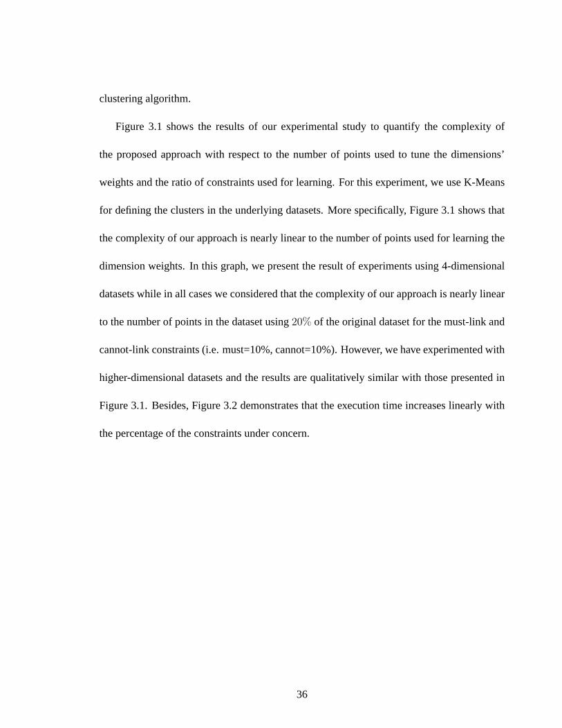
Figure 3.1 shows the results of our experimental study to quantify the complexity of

the proposed approach with respect to the number of points used to tune the dimensions’

weights and the ratio of constraints used for learning. For this experiment, we use K-Means

for defining the clusters in the underlying datasets. More specifically, Figure 3.1 shows that

the complexity of our approach is nearly linear to the number of points used for learning the

dimension weights. In this graph, we present the result of experiments using 4-dimensional

datasets while in all cases we considered that the complexity of our approach is nearly linear

to the number of points in the dataset using20% of the original dataset for the must-link and

cannot-link constraints (i.e. must=10%, cannot=10%). However, we have experimented with

higher-dimensional datasets and the results are qualitatively similar with those presented in

Figure 3.1. Besides, Figure 3.2 demonstrates that the execution time increases linearly with

the percentage of the constraints under concern.

36

Chapter 4

Experimental Evaluation

In this section, we test our approach with a comprehensive set of experiments. In Section 4.1,

we discuss the dataset we used for experimental purpose and the accuracy measure based on

which we evaluate the clustering performance of our approach. In Section 4.2.1, we show

simple experiments which requires subjective evaluation, but strongly hints at the value of

our approach. We show how well we can meet the user requirements, which other exist-

ing clustering methods could not achieve. In Section 4.2.2, we present a comparison of

our method with both a related approach proposed in literature and with the unsupervised

clustering method. In Section 4.2.3 we show how our Hill Climbing method contributes in

improving the clustering results. And finally, in section 4.3, we present the results of apply-

ing our method on two real-time dataset. Section 4.3.1 demonstrates the result of the weather

sensor data sets and section 4.3.2 presents the clustering obtained for bees’ data set.

37

Figure 4.1: The original Dataset, where data are distributed around the lines A, B and C

4.1 Methodology and Datasets

We used MATLAB to implement our approach and we experimented with various datasets

and clustering algorithms. To show the advantage of our approach with respect to unsuper-

vised learning we used some synthetic datasets, generated to show the indicative cases where

unsupervised clustering fails to find the clusters that corresponds to the user intention. We

also used datasets from the UC Irvine repository1 to evaluate the effectiveness of our method

with respect to a pre-specified clustering method in which the same dataset were used.

4.1.1 Clustering Accuracy

Rand statistic [33] is an external cluster validity measure which estimates the quality of the

clustering with respect to a given clustering structure of the data. It measures the degree

of correspondence between a prespecified structure, which reflects our intuition of a good

1http://www.ics.uci.edu/ mlearn/MLRepository.html

38

Figure 4.2: Clustering of Original Dataset using Kmeans

Figure 4.3: Clustering of Original Dataset in the new space using our approach

39

Figure 4.4: Projection of the clusters presented in figure 4.3 to the original space

clustering of the underlying dataset, and the clustering results after applying our approach to

X. Let C = {c1, . . . , cr} be a clustering structure of a datasetX into r clusters andP =

{P1, . . . , Ps} be a defined partitioning of the data. We refer to a pair of points(xv, xu) ∈ X

from the data set using the following terms:

• SS: if both points belong to the same cluster of the clustering structure C and to the

same group of partition P.

• SD: if points belong to the same cluster of C and to different groups of P.

• DS: if points belong to different clusters of C and to the same group of P.

• DD: if both points belong to different clusters of C and to different groups of P.

Assuming now thata, b, c andd are the number ofSS, SD,DS andDD pairs respectively,

thena + b + c + d = M which is the maximum number of all pairs in the data set (meaning,

M = n · (n− 1)/2 wheren is the total number of points in the data set).Now we can define

40

the Rand Statistic index to measure the degree of similarity betweenC andP as follows:

R = (a + d)/M

4.2 Results and Discussion

4.2.1 Semi-supervised vs. unsupervised learning

Referring to Figure 1.1 again, we applied our method to satisfy the user constraints that the

group B and C should belong to the same cluster. Figure 1.3 shows clustering results in

the modified space using our technique, whereas Figure 1.4 shows the projection of clusters

obtained in Figure 1.3 in the original dimensions.

The visualization of a similar example is presented in Figure 4.1. One can claim that there

are three groups of data as defined by the three lines A, B and C as Figure 4.1 depicts. We

apply K-Means [24] to partition it into three clusters. The result of unsupervised K-Means is

presented in Figure 4.2. It is clear that K-Means is not able to identify the three clusters that

the user asked for. Given a set of constraints, we applied our approach. Figure 4.3 shows the

projection of the dataset and its clustering to a new space, while Figure 4.4 demonstrates the

projection of clusters in the original space.

41

0.9 0.91 0.92 0.93 0.94 0.95 0.96 0.97 0.98 0.99

1

2 4 6 8 10 12 14 16 18 20

Acc

urac

y (R

ando

m S

tatis

tics)

% of Constraints

Iris Dataset

Kmeans+our approachKmeans+diagonal matrix

Figure 4.5: Clustering Accuracy Vs Constraints IRIS dataset

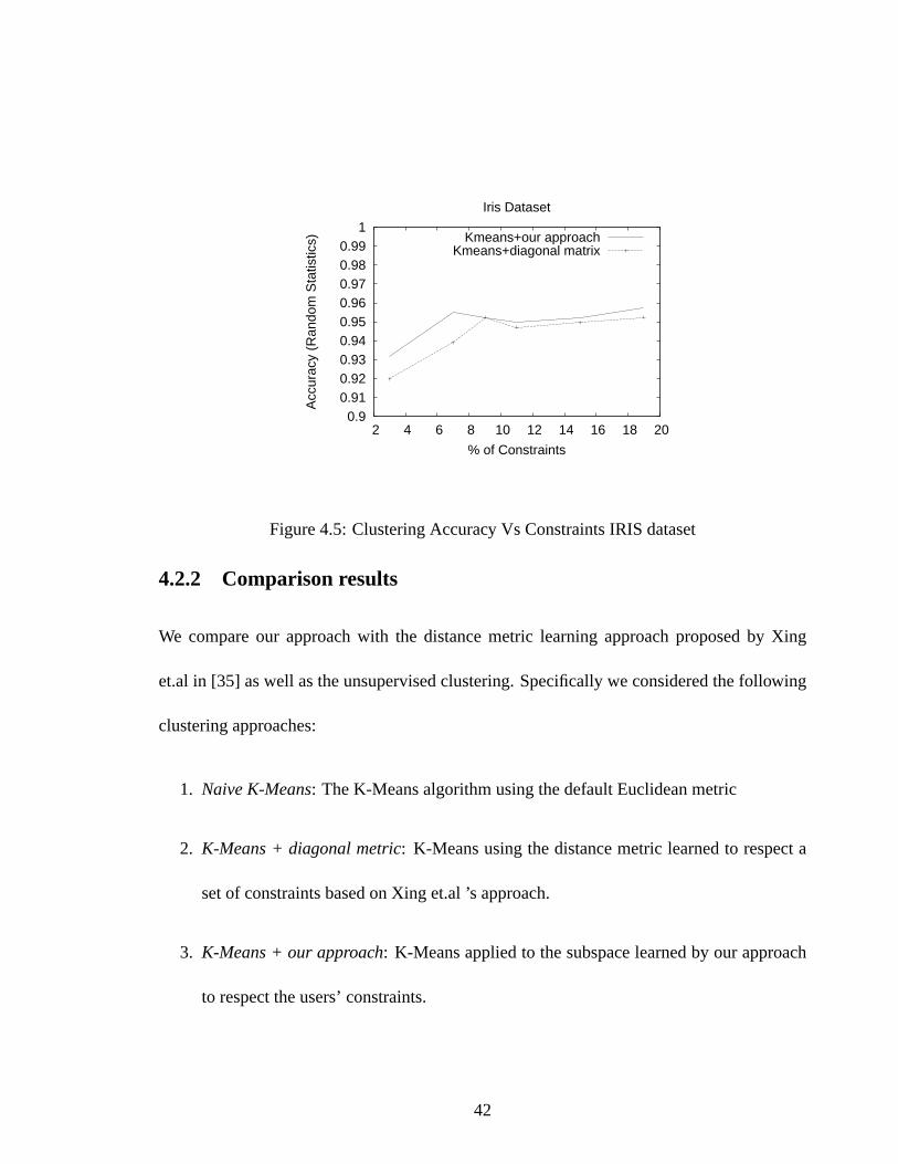
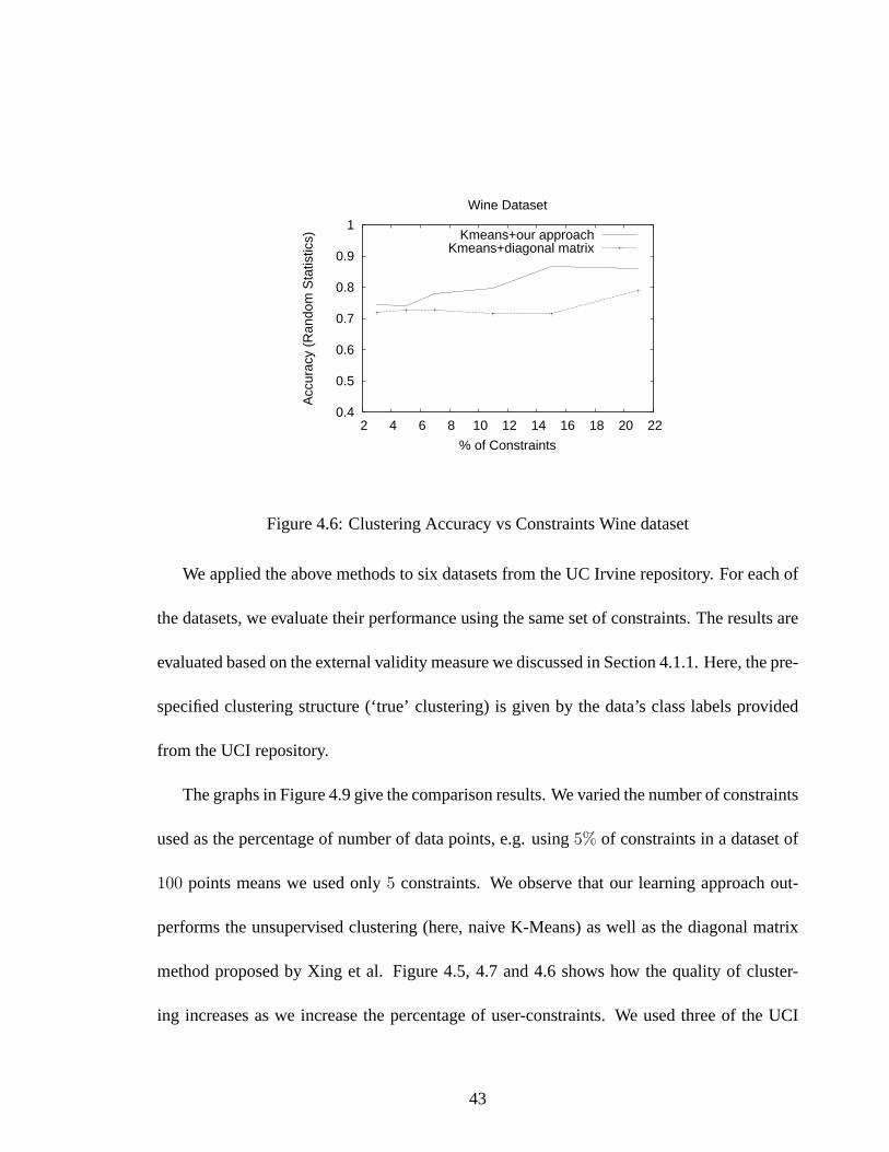
4.2.2 Comparison results

We compare our approach with the distance metric learning approach proposed by Xing

et.al in [35] as well as the unsupervised clustering. Specifically we considered the following

clustering approaches:

1. Naive K-Means: The K-Means algorithm using the default Euclidean metric

2. K-Means + diagonal metric: K-Means using the distance metric learned to respect a

set of constraints based on Xing et.al ’s approach.

3. K-Means + our approach: K-Means applied to the subspace learned by our approach

to respect the users’ constraints.

42

0.4

0.5

0.6

0.7

0.8

0.9

1

2 4 6 8 10 12 14 16 18 20 22

Acc

urac

y (R

ando

m S

tatis

tics)

% of Constraints

Wine Dataset

Kmeans+our approachKmeans+diagonal matrix

Figure 4.6: Clustering Accuracy vs Constraints Wine dataset

We applied the above methods to six datasets from the UC Irvine repository. For each of

the datasets, we evaluate their performance using the same set of constraints. The results are

evaluated based on the external validity measure we discussed in Section 4.1.1. Here, the pre-

specified clustering structure (‘true’ clustering) is given by the data’s class labels provided

from the UCI repository.

The graphs in Figure 4.9 give the comparison results. We varied the number of constraints

used as the percentage of number of data points, e.g. using5% of constraints in a dataset of

100 points means we used only5 constraints. We observe that our learning approach out-

performs the unsupervised clustering (here, naive K-Means) as well as the diagonal matrix

method proposed by Xing et al. Figure 4.5, 4.7 and 4.6 shows how the quality of cluster-

ing increases as we increase the percentage of user-constraints. We used three of the UCI

43

0.3

0.4

0.5

0.6

0.7

0.8

0.9

1

2 4 6 8 10 12 14 16 18 20

Acc

urac

y (R

ando

m S

tatis

tics)

% of Constraints

Diabetes Dataset

Kmeans+our approachKmeans+diagonal matrix

Figure 4.7: Clustering Accuracy vs Constraints Diabetes dataset

0.4

0.5

0.6

0.7

0.8

0.9

1

0 2 4 6 8 10 12 14

Acc

urac

y (R

and

Sta

tistic

)

Number of Dimensions

Wine Dataset (Constraints: Must=5%, Cannot=6%)

Figure 4.8: Clustering Accuracy vs Dimensions for Wine dataset

44

datasets (Iris, Wine and Protein) to show the performance of our learning approach in com-

parison to learning a diagonal matrix as proposed in [35]. We note that in all the three cases

our approach gives a significant improvement. Moreover, it appears to learn the subspace

where a good clustering can be found quickly with only a small number of constraints. For

example, in case of the Wine dataset, only with10% of constraints, we get an accuracy close

to 0.8 using our approach which the Xing et.al’s approach cannot achieve even with more

constraints. Similar results can also be observed for the other datasets.

Also, we evaluate the performance of our approach (in terms of the clustering accuracy)

in relation to the dimensionality of the space where the clustering is defined. For instance,

Figure 4.8 shows how the quality of clustering for the Wine dataset changes with the number

of dimensions. We observe that the clustering accuracy increases as the number of dimen-

sions increases from two to five while it remains vaguely the same for higher dimensions.

This implies that, in case of Wine, the use of more than five dimensions does not seem to

improve the quality of the defined clusters and thus tuning only five of the twelve dimensions

our approach can lead to a good clustering of the Wine data. Experiments with other UCI

datasets lead to similar results. Based on these observations, it is obvious that our approach

does not only learn the data dimensions to satisfy the user constraints but it also assists with

selecting the subspace where the ‘best’ clustering can be defined.

45

Figure 4.9: Clustering Accuracy on UCI datasets

46

4.2.3 Advantage of Hill Climbing method

This experiment was done with wine dataset, which consists of168 points,12 dimensions and

3 clusters. We applied K-Means to this dataset and got an accuracy of71.86%. The clustering

result is shown in Figure 4.10. Please note that the data is projected in3 dimensions using

Multi Dimensional Scaling (MDS) for the visualization purpose.

We applied K-Means with Diagonal metric giving some must link and cannot link con-

straints and the clustering results obtained is shown in the figure 4.11. The accuracy observed

was84.73%.

Finally, in order to observe the effect of clustering results by applying Hill Climbing

method, we tuned the weight of dimensions obtained by the diagonal metric learned above.

We obtained an improved accuracy of91.7%. The clustering result is shown in Figure 4.12.

Its clearly visible that the hill climbing method finds out an optimal weight of the dimen-

sions, which helps in obtaining better clustering results.

4.3 Real Time Datasets

To demonstrate how our approach can help with a real world problem, especially in large

unlabeled dataset, we performed experiments with the following two real datasets. Section

4.3.1 demonstrates the clustering results obtained on the Pacific Northwest weather data and

section 4.3.2 demonstrates the clustering results of a dataset obtained from bee’s olfactory

system.

47

Figure 4.10: MDS 3-dimension plot of K-Means clustering results for Wine Dataset (3 clus-ters)

Figure 4.11: MDS 3-dimension plot of clustering using K-Means Diagonal metric for WineDataset (3 clusters)

48

Figure 4.12: MDS 3-dimension plot of clustering after applying Hill Climbing method onthe Diagonal metric for Wine Dataset (3 clusters)

4.3.1 Weather Dataset

First experiment we performed was with the live data from K-12 Educators [10]. The data

was obtained from32 temperature sensors placed at various locations in Pacific Northwest

states (Washington and Oregon). The sensors recorded temperatures at a regular interval of

12 hour. We took a set of100 consecutive readings from each sensors which made it 32 time

series of length100. We aimed to cluster the time periods for those times, when the average

temperature of some sensors were more than the others. Figure 4.13 demonstrates the desired

clustering. It shows the time-periods divided into two clusters. In order to achieve this clus-

tering, we applied unsupervised K-Means (withk=2) and we obtained the result presented in

Figure 4.14. We observe that K-Means partitioned the data into two parts, not the way we

wanted them to be. We then applied our semi-supervised approach on the dataset and pro-

49

Figure 4.13: The desired clustering of weather dataset

Table 4.1: Accuracy applying unsupervised Clustering on Weather Dataset Figure 4.13Clustering Approach Accuracy

Unsupervised K-Means0.49Semi-supervised .80

vided some must and cannot constraints. The clustering result we got is presented in Figure

4.15. It’s clear that our approach clustered the data set in a better way. The accuracy obtained

is shown in table 4.1. Please note that the high-dimensional dataset n Figures 4.134.144.15

are plotted using Multi Dimensional Scaling (MDS) for visualization purpose.

50

Figure 4.14: The clustering results of weather dataset using unclustered K-Means, k=2

Figure 4.15: The clustering results of weather dataset using our approach

51

4.3.2 Bees Dataset

We clustered the optical recording data from a bee’s olfactory system to help us understand-

ing the mechanisms of the olfactory code and the temporal evolution of activity patterns in the

antennal lobe of bees. The data consists of980 images, each image containing688X520 pix-

els. Considering each pixel as a time series, the data consists of357, 760 time series of length

980. We used K-Means to cluster this dataset (withk set to15) with the objective to cluster

the series with similarity in time. Figure 4.16 shows the clusters obtained by K-Means.

In order to apply our method to this dataset, we defined a method to generate the con-

straints automatically. We cluster the data first using K-Means with a large value ofk (say

100) and then we specify the must-link constraints as those points which belong to the same

clusters whereas cannot-link constraints as those points which belongs to clusters that are far

apart. After obtaining the constraints, we applied our technique to get the clustering results

for 15 results. Figure 4.17 shows the15 clusters that we obtained.

52

Figure 4.16: The clustering results of bees dataset using K-Means, k=15

Figure 4.17: The clustering results of bees dataset using Our approach, k=15

53

Chapter 5

Conclusions

Clustering is not a totally resolved problem and the quality of its results is rather difficult

to be assessed since there is no previous knowledge of the underlying data structure. Hence

depending on the application domain and /or the user perspective different partitioning of a

data set can be considered to be a good clustering. An important challenge in clustering is

the definition of clusters in the underlying dataset so that user intention is satisfied. In this

thesis, we have introduce an approach for learning the space where the ‘best’ partitioning

of the underlying data based on the user constraints can be defined. It is a semi-supervised

learning approach that aims to efficiently combine both objective (i.e. related to the data

structure) and subjective (i.e. user constraints) criteria in the context of clustering. The pro-

posed approach allow the user to guide the clustering process by providing some constraints

and giving his/her feedback during the whole clustering process. Moreover, it selects the

dimensions that seem to contribute to the clustering process while it also gives some weights

54

to the dimensions under concern so that the best partitioning of the data is defined accord-

ing to the user constraints. Hence a data projection to a new space that respects the given

constraints is defined. The weighted dimensions also assist with the definition of a proper

distance measure which will reflect the indicated by the user clustering preferences. The

weights are learned based on a hill climbing (HC) method. The quality criterion of the HC

method relies on acluster validity indexthat reflects the objective evaluation of the defined

clusters and ameasure of the clusters accuracyin relation with the user constraints. Our

approach can be used in conjunction of any unsupervised clustering algorithm providing an

significant improvement to their results. Our experimental results using both real and syn-

thetic datasets show that our approach enables significant improvements in the accuracy of

the defined clustering with respect to the user constraints.

55

Bibliography

[1] C. Aggarwal and P. S. Yu. Finding generalized projected clusters in high dimensionalspaces. InProceedings of the ACM SIGMOD International Conference on Managementof Data, 2000.

[2] Brigham Anderson, Andrew Moore, and David Cohn. A nonparametric approach tonoisy and costly optimization. InInternational Conference on Machine Learning, 2000.

[3] K.P.Bennett Ayhan Demiriz and M.J.Embrechts. Semi-supervised clustering using ge-netic algoeithm. InProceedings of ANNIEB(Artificial Neural Netowrks in Engineer-ing), November 1999.

[4] A. Bar-Hillel, T. Hertz, N. Shental, and D. Weinshall. Learning distance function usingequivalence relations. InProceedings of the 12th International Conference on MachineLearning (ICML-2003), 2003.

[5] S. Basu, M. Bilenko, and R. J. Mooney. A probabilistic framework for semi-supervisedclustering. InProceedings of the 10th ACM SIGKDD International Conference onKnowledge Discovery and Data Mining (KDD-2004), August 2004.

[6] M. Berry and G. Linoff. Data Mining Techniques for Marketin: Sale and Customersuppeort. John Willey and Sons, Inc., 1996.

[7] Ming-Syan Chen Bi-Ru Dai, Cheng-Ru Lin. On the techniques of data clustering withnumerical constraints. InIn Proceedings of SIAM International Conference on DataMining, 2003.

[8] A. Blum and T. Mitchell. Combining labeled and unlabeled data with co-training. InProceedings of the 11th Anual Conference on Computational Learning Theory, pages92–100, 1998.

[9] Aggarwal C., Procopiuc C., Wolf J., Yu P., and Park J. Fast algorithms for projectedclustering. InProceedings roceedings of the ACM SIGMOD International Conferenceon Management of Data, 1999.

[10] Earth Climate, NASA’s IITA Program Weather, K-12 Educators, and Universityof Washington. http://www-k12.atmos.washington.edu/k12/grayskies.

56

[11] D. Cohn, R. Caruana, and A. McCallum. Semi-supervised clustering with user feed-back. InTechnical Report TR2003-1892, 2003.

[12] S. D. Kamvar D. Klein and C. Manning. From instance-level constaraints to space-levelconstraints. making the most of prior knowledge in data clustering. InProceedingsof the 19th International Conference on Machine Learning. ICML, Sydney, Australia,2002.

[13] C. Domeniconi and Dimitrios Gunopulos. Adaptive nearest neighbor classifications us-ing support vector machines. InIn Advances in Neural Information Processing Systems14.MIT Press, 2002.

[14] M. Ester, H.-P. Kriegel, J. Sender, and X. Xu. Sensity-connected sets and their appli-cation for trend detection in spatial databases. InProceedings of Int. Conf. KnowledgeDiscovery and Data Mining, pages 10–15, August 1997.

[15] U. Fayyad, P. Smuth G. Piatesky-Shapiro, and R. Uthurusamy.Advance in KnowledgeDiscovery and Data Mining. AAI Press, 1996.

[16] Fisher and Douglas. Knowledge acquisition via incremental conceptual clustering.Ma-chine Learning, 2:139–172, 1987.

[17] Maria Halkidi and Michalis Vazirgiannis. Clustering validity assessment: Finding theoptimal partitioning of a data set. InProceedings of the ICDM Conference, 2001.

[18] Eui-Hong Han, George Karypis, Vipin Kumar, and Bamshad Mobasher. Hypergraphbased clustering in high-dimensional data sets: A summary of results.IEEE Data Eng.Bull., 21(1):15–22, 1998.

[19] T. Hastie and R. Tibshirani. Discriminant adaptive nearest neighbor classification.In IEEE transactions on Pattern Analysis and Machine Learning, pages 18:607–616,1996.

[20] T. Hastie, R. Tibshirani, and J Friedman.The Elements of Statistical Learning: DataMining, Inference and Prediction. Springer, 2003.

[21] A. Hinneburg and D. Keim. An efficient approach toclustering in large multimediadatabases with noise. InProceedings of Int. Conf. Knowledge Discovery and DataMining, pages 58–65, August 1998.

[22] T.S. Jaakkola and D. Haussler. Exploiting generative models in a discriminative clas-sifier. In In Proceedings of Tenth Conference on Advances in Neural Information Pro-cessing System, 1999.

[23] A.K. Jain, M.N. Mutty, and P.J Flyn. Data clustering: A review.ACM ComputingSurveys, 31(3), 1999.

57

[24] MacQueen J.B. Some methods for classification and analysis of multivariate observa-tions. InProceedings of the 5th Symposium on Math, Statistic and Probability, pages281–297. Berkeley, CA: University of California Press, 1967.

[25] Wagstaff K. and Cardie. Clustering with instance-level constraints. InProceedings ofthe 17th International Conference on Machine Learning, 2000.

[26] A. Blum N. Bansal and S. Chawla. Correlation clustering. InProceedings of the 43rdIEEE symposium on Foundations of Computer Science, pages 238–247, 2002.

[27] A. Y. Ng, M. Jordan, and Y. Weiss. On spectral clustering: Analysis and an algorithm.Advances in in Neural Information Processing Systems, 2001.

[28] K. Nigam, K. McCallum, S. Thrun, and T. Mitchell. Text classification labeled andunlabeled documents using em.Machine Learning, 39:103–134, 2000.

[29] W. H. Press, S. A. Teukolsky, W. T. Vetterling, and B. P. Flannery.Numerical Recipesin C, The art of Scientific Computing. Cambridge University Press, 1997.

[30] Agrawal R., Gehrke J., Gunopulos D., and Raghavan P. Automatic subspace clusteringof high dimensional data for data mining applications. InProceedings roceedings of theACM SIGMOD International Conference on Management of Data, 1998.

[31] E. Segal, H. Wang, and D. Koller. Discovering molecular pathways from protein inter-action and gene expression data.Bioinformatics, 19:264–272, July 2003.

[32] Benno Stein, Sven Meyer zu Eissen, and Frank Wibrock. On cluster validity and theinformation need of users. InProceedings of the 3rd Int. Conference on Artificial Intel-ligenece and Applications, September 2003.

[33] S. Theodoridis and K. Koutroubas.Pattern Recognition. Academic Press, 1999.

[34] K. Wagstaff, C. Cardie, S. Rogers, and S. Schroedl. Constrained k-means clusteringwith background knowledge. InProceedings of 18th International Conference on Ma-chine Learning (ICML-2001), pages 577–584, 2001.

[35] Eric P. Xing, Andrew Y. Ng, Michael I. Jordan, and Stuart Russell. Distance metriclearning, with application to clustering with side-information. InProceedings of theNeural Information Processing Systems (NIPS) Conference, December 2002.

58

Appendix A

Source code

This section contains the source code for semi-supervised learning framework. Thecode is written in MATLAB.

%%%%%%%%%%%%%%%%%%%%%%%%%%%%%%%%%%%%%%%%% Main Program: Semisupervised Learning Framework %% %%%%%%%%%%%%%%%%%%%%%%%%%%%%%%%%%%%%%%%%%

% Copyright and terms of use (DO NOT REMOVE): The code is made freely% available for non-commercial uses only, provided that the copyright% header in each file not be removed, and suitable citation(s)(see below)% be made for the author’s work.%% The code is not optimized for speed, and we are not responsible for any% errors that might occur in the code.%% The copyright of the code is retained by the authors. By downloading,% using this code you agree to all the terms stated above.%% This Program is a framework for semi-supervised learning using subjective% and objective cluster validity criterion. For a given multi-dimension% dataset, this program finds out the best possible clustering. It is an% interactive program, which takes user’s feedback at each step. For% experimental purpose, I have made the feedback process fully automated.% This program assumes that the Must-link and can-not link are stored in% files must.txt and mustnot.txt respectively.%%% Input:% original data is a variable name which contains the labeled data% to be clustered with labels in the last column.

59

% maxcluster is the number of clusters the user wants to group% the data into.% hc flag to choose if the user wants to apply Hill% Climbing method.% Output:%% The clustering results at every dimension stored in the result.txt file% as well as the 2-dimension MDS plot of the best clustering result.%% Copyright (c) 2005, Nitin Kumar, All rights reserved.

function semisupervised learning(original data,maxcluster,hc,x)

% Opening the file for writing the outputffd1= fopen( ’result.txt’ , ’w’ );

% Since the last column contains the labels, extract the data without label% and put it in variable x.for tt= (1:size(original data,2)-1)

x(:,tt)=original data(:,tt);end

to cluster=maxcluster;

% Initial clusteringtno= size(x,1);oldx=x;

% Apply SVD to get the initial weights of each dimensions.[s u v]=svd(x);

%define a variable which decide the no of initial dimensions to start with.dim=2;

%Generate a new matrix and initialize it to zeros.u1=zeros(size(u,1), size(u,2));

%Find out the possible number of dimensionsmaxdim= size(u,2);

% Fill the matrix generated above with the ”dim” dimensions value.for i = (1:dim)

60

u1(i,i)=u(i,i);end

% Combine the dimensions u1 with s to get the data in a new spacex=s*u1*v’;

%Cluster this new data and present it to the user% Constructing the matrix S (tno x tno)S=zeros(tno,tno);D=zeros(tno,tno);

% Take user feedback and apply Newton Raphson method% Asking user for the feedback and reconstructing the Matrices

must=load( ’must.txt’ );for in=(1:size(must,1))

S(must(in,1),must(in,2))=1;S(must(in,2),must(in,1))=1;

end

mustnot=load( ’mustnot.txt’ );for in=(1:size(mustnot,1))

D(mustnot(in,1),mustnot(in,2))=1;D(mustnot(in,2),mustnot(in,1))=1;

end

% These variables stores the best accuracy and the corresponding dimension.best(1)=0; best(2)=0;

% This loop iterates the number of dimensions times.while ( dim <= maxdim )

initialx=oldx;% Applying Newton Raphson’s methodcluster iteration= maxcluster;y1=newton(x,S,D,1);z1=y1*x’;clear r; clear U; clear a; clear yy; clear y;% K-Means clusteringU=kmeans(z1’,cluster iteration);w=U’;for row= (1:size(w,1))

for col = (1:size(w,2))if (w(row,col) == 1)

61

yy(row)=col;end

endendy=yy’;for in= (1:maxcluster)

k=1;for j= (1: size(y,1))

if (y(j) == in)a{in }(k)=j;k=k+1;

endend

end

% Applying Hill Climbing method to obtain the optimal weightsfor in= (1: dim)

weights(in)=y1(in,in);end

if (hc == 1)acc= accuracy(original data,a,maxcluster);if (best(1) < acc)

best(1)=acc;best(2)=dim;

endfor i= (1: size(weights,2))

step=0.1*weights(i);old index=cluster validity(z1’,cluster iteration,a);old accuracy=constraint accuracy(must,mustnot,

a,maxcluster);weights(i)=weights(i)+step;

%Regenerating y1 matrix and new clusterings out of the new weightsfor m=(1:size(weights,2))

y1(m,m)=weights(m);endz1=y1*x’;clear r; clear U; clear a; clear yy; clear y;U=kmeans(z1’,cluster iteration);w=U’;for row= (1:size(w,1))

for col = (1:size(w,2))

62

if (w(row,col) == 1)yy(row)=col;

endend

endy=yy’;for in= (1:maxcluster)

k=1;for j= (1: size(y,1))

if (y(j) == in)a{in }(k)=j;k=k+1;

endend

endnewdata=z1’;for m= (1:cluster iteration)

for c= (1:size(a {m},2))newdata(a {m}(c),size(oldx,2)+1)=m;

endendclear newdata;

%Calculating the new validity indexnew index=cluster validity(z1’,cluster iteration,a);new accuracy=constraint accuracy(must,mustnot,

a,maxcluster);if ((100*new accuracy+(1/(new index+eps)))

>(100*old accuracy+(1/(old index+eps))))while ((100*new accuracy+(1/(new index+eps)))

>(100*old accuracy+(1/(old index+eps)))),weights(i)=weights(i)+step;old index= new index;old accuracy= new accuracy;%Regenerating y1 matrix and new clusterings out of the%new weightsfor m=(1:size(weights,2))

y1(m,m)=weights(m);endz1=y1*x’;clear r; clear U; clear a; clear y;U=kmeans(z1’,cluster iteration);w=U’;for row= (1:size(w,1))

63

for col = (1:size(w,2))if (w(row,col) == 1)

yy(row)=col;end

endendy=yy’;for in= (1:maxcluster)

k=1;for j= (1: size(y,1))

if (y(j) == in)a{in }(k)=j;k=k+1;

endend

end

%Calculating the new validity indexnew index= cluster validity(z1’, cluster iteration, a);new accuracy= constraint accuracy(must,mustnot,a,maxcluster);

if (( (100*new accuracy + (1/(new index+eps)))< (100*old accuracy +(1/(old index+eps))))&((weights(i)- step)>= 0))weights(i)=weights(i)- step;

endend % End of while (newindex ¡ old index)

elseif ((weights(i)- 2*step) > 0 )weights(i)= weights(i)-2*step;for m=(1:size(weights,2))

y1(m,m)=weights(m);endz1=y1*x’;clear r; clear U; clear a; clear yy; clear y;U=kmeans(z1’,cluster iteration);w=U’;for row= (1:size(w,1))

for col = (1:size(w,2))if (w(row,col) == 1)

yy(row)=col;end

endendy=yy’;

64

for in= (1:maxcluster)k=1;for j= (1: size(y,1))

if (y(j) == in)a{in }(k)=j;k=k+1;

endend

end%Calculating the new validity indexnew index= cluster validity(z1’, cluster iteration, a);new accuracy= constraint accuracy(must,mustnot,a,maxcluster);

if ((100*new accuracy + (1/(new index+eps)))> (100*old accuracy+(1/(old index+eps))))while (( (100*new accuracy + (1/(new index+eps)))

> (100*old accuracy+(1/(old index+eps))))& ((weights(i)-step) >= 0 )),weights(i)=weights(i)- step;old index= new index;old accuracy= new accuracy;

%Regenerating y1 matrix and new clusterings out of the new weightsfor m=(1:size(weights,2))

y1(m,m)=weights(m);endz1=y1*x’;clear r; clear U; clear a; clear yy; clear y;U=kmeans(z1’,cluster iteration);w=U’;for row= (1:size(w,1))

for col = (1:size(w,2))if (w(row,col) == 1)

yy(row)=col;end

endendy=yy’;for in= (1:maxcluster)

k=1;for j= (1: size(y,1))

if (y(j) == in)a{in }(k)=j;k=k+1;

end

65

endend

%Calculating the new validity indexnew index= cluster validity(z1’, cluster iteration, a);new accuracy= constraint accuracy(must,mustnot,a,maxcluster);

if ( (100*new accuracy+ (1/(new index+eps)))< (100*old accuracy+(1/(old index+eps))))weights(i)=weights(i)+ step;end

end % End of while ( newindex ¡ old index)else

weights(i)=weights(i)+step;end % End of if- else

elseweights(i)=weights(i)-step;end % End of first if - elseend % End of for iteration of weights

for m=(1:size(weights,2))y1(m,m)=weights(m);

endz1=y1*x’;clear r; clear U; clear a; clear yy; clear y;U=kmeans(z1’,cluster iteration);w=U’;for row= (1:size(w,1))

for col = (1:size(w,2))if (w(row,col) == 1)

yy(row)=col;end

endendy=yy’;for in= (1:maxcluster)

k=1;for j= (1: size(y,1))

if (y(j) == in)a{in }(k)=j;k=k+1;

endend

endacc= accuracy(original data,a,maxcluster);if (best(1) < acc)

66

best(1)=acc;best(2)=dim;

endend % If condition for HC method

for m=(1:size(weights,2))y1(m,m)=weights(m);

endz1=y1*x’;clear r; clear U; clear a; clear yy; clear y;U=kmeans(z1’,cluster iteration);w=U’;for row= (1:size(w,1))

for col = (1:size(w,2))if (w(row,col) == 1)

yy(row)=col;end

endendy=yy’;for in= (1:maxcluster)

k=1;for j= (1: size(y,1))

if (y(j) == in)a{in }(k)=j;k=k+1;

endend

endacc= accuracy(original data,a,maxcluster);if (best(1) < acc )

best(1)=acc;best(2)=dim;

endfprintf(ffd, ’%d\t%f \n’ , dim, acc);dim=dim+1;

if (dim <= maxdim)for i = (1:dim)

u1(i,i)=u(i,i);endx=s*u1*v’;

end

67

end % End of main while loop% Printing out the dimension with the best resultsfprintf(ffd, ’%f \t%d\n’ ,best(1),best(2));% Plotting the clusters in the modified spacemdsmodify(z1’,a, maxcluster);% Plotting the clusters in the original spacemdsmodify(oldx,a, maxcluster);fprintf(ffd, ’I am done with all %d dimensions \n’ ,dim);

%%%%%%%%%%%%%%%%%%%%%%%%%%%%%%%%%%%%%%%%% This function calculates the accuracy of the %% clustering results obtained. %%%%%%%%%%%%%%%%%%%%%%%%%%%%%%%%%%%%%%%%%

function score = accuracy(data,C,maxcluster)%If the cluster number is represented as 0, then increment%all the cluster numbers by 1.last column = size(data,2);flag=0;for i=(1:size(data,1))

if (data(i,last column) == 0)flag = 1;

endendif (flag == 1)

for i=(1:size(data,1))data(i,last column)= data(i,last column) + 1;

endend

%Extracting the partitioning P from the given datafor i= (1:maxcluster)

P{i }=0;end

for i= (1:maxcluster)k=1;for j=(1:size(data,1))

if (data(j,last column) == i)P{i }(k)=j;k=k+1;

end

68

endend

%Finding out SS, SD, DS and DD from all possible pairs of points%int he dataset.pair1(size(data,1),size(data,1))=zeros;for i= (1: maxcluster)

for j= (1:size(P {i },2)-1)for k= (j+1:size(P {i },2))

pair1(P {i }(j),P {i }(k))= 1;pair1(P {i }(k),P {i }(j))= 1;

endend

end

pair2(size(data,1),size(data,1))=zeros;for i= (1: maxcluster)

for j= (1:size(C {i },2)-1)for k= (j+1:size(C {i },2))

pair2(C {i }(j),C {i }(k))= 1;pair2(C {i }(k),C {i }(j))= 1;

endend

end

a=0;b=0;c=0;d=0;for i=(1:size(data,1)-1)

for j=(i+1:size(data,1))%finding out if these two point belongs to same Clusterif ( (pair1(i,j) ==1) & (pair2(i,j) == 1))

a=a+1;endif ( (pair1(i,j) ==1) & (pair2(i,j) == 0))

c=c+1;endif ( (pair1(i,j) ==0) & (pair2(i,j) == 1))

b=b+1;endif ( (pair1(i,j) ==0) & (pair2(i,j) == 0))

d=d+1;

69

endend

end

M= a+b+c+d;R= (a+d)/M;J= (a/(a+b+c));score=R;

%%%%%%%%%%%%%%%%%%%%%%%%%%%%%%%%%%%%%%%%% This function converts an array nxm to Vector %%%%%%%%%%%%%%%%%%%%%%%%%%%%%%%%%%%%%%%%%

%Input: X=Dataset%function DATA= ArrToVector(X)import java.util.Vector;[m, dim] = size(X);data = Vector;for i = (1:m)

data i = Vector;for j = (1:dim)

data i.addElement(X(i,j));enddata.addElement(data i);

endDATA = Vector;DATA = data;

%vector containing the locations of points that belong to each%of the cl clusters.%Input: X= data and clusters id, cl= number of clusters

function Clusters v= Clustervector(X,cl)import java.util.Vector;[m, dim] = size(X);for i = (1:cl)

cluster v (i)= java.util.Vector;endfor i = (1:m)

loc =X(i, dim);cluster v(loc).addElement(i-1)

end

70

Clusters v = cluster v;

%%%%%%%%%%%%%%%%%%%%%%%%%%%%%%%%%%%%%%%%% This function calculates the accuracy wrt user constraints %%%%%%%%%%%%%%%%%%%%%%%%%%%%%%%%%%%%%%%%%

function score=constraint accuracy(must,mustnot,C,maxcluster)size1= size(must,1);size2=size(mustnot,1);

counter=0;for i = (1: size1)

x1=must(i,1);x2=must(i,2);for j= (1: maxcluster)

flag1=0;flag2=0;for k= (1:size(C {j },2))

if ( C{j }(k) == x1)flag1=1;

endif ( C{j }(k) == x2)

flag2=1;end

endif ((flag1 == 1) & (flag2 == 1))

counter=counter+1;end

endend

counter=counter+size2;

for i = (1: size2)x1=mustnot(i,1);x2=mustnot(i,2);for j= (1: maxcluster)

flag1=0;flag2=0;for k= (1:size(C {j },2))

if ( C{j }(k) == x1)flag1=1;

end

71

if ( C{j }(k) == x2)flag2=1;

endendif ((flag1 == 1) & (flag2 == 1))

counter=counter-1;end

endend

score= (counter/(size1+size2));%%%%%%%%%%%%%%%%%%%%%%%%%%%%%%%%%%%%%%%%% This function automatically generates the constraints and %% store them in must.txt and mustnot.txt files. %%%%%%%%%%%%%%%%%%%%%%%%%%%%%%%%%%%%%%%%%

function create constraints(data,maxcluster,percentage1,percentage2)

%If the cluster number is represented as 0, then increment%all the cluster numbers by 1.last column = size(data,2);flag=0;for i=(1:size(data,1))

if (data(i,last column) == 0)flag = 1;

endendif (flag == 1)

for i=(1:size(data,1))data(i,last column)= data(i,last column) + 1;

endend

% Initialize Pfor i= (1:maxcluster)

P{i }=0;end% Copy Cluster Information in the variable P.for i= (1:maxcluster)

k=1;for j=(1:size(data,1))

if (data(j,size(data,2)) == i)P{i }(k)=j;

72

k=k+1;end

endend%Open Must file for writingfid=fopen( ’must.txt’ , ’w’ );for i= (1: maxcluster)

points=round(percentage1*(size(P {i },2)));rand points= rand gen(1,size(P {i },2),points);for j= (1:points-1)

fprintf(fid, ’%d\t%d’ ,P {i }(rand points(j)),P{i }(rand points(j+1)));fprintf(fid, ’ \n’ );

endendfclose(fid);

%percentage2=.4;%Open Msut Not file for writingfid=fopen( ’mustnot.txt’ , ’w’ );for i= (1: maxcluster-1)

m=i+1;len1=size(P {i },2);len2=size(P {m},2);mini=min(len1,len2);points=round(percentage2*mini);rand points1= rand gen(1,size(P {i },2),points);rand points2= rand gen(1,size(P {m},2),points);for j= (1:points-1)

fprintf(fid, ’%d\t%d’ ,P {i }(rand points1(j)),P{m}(rand points2(j)));fprintf(fid, ’ \n’ );

endendfclose(fid);%%%%%%%%%%%%%%%%%%%%%%%%%%%%%%%%%%%%%%%%% This function automatically generates random numbers %% %%%%%%%%%%%%%%%%%%%%%%%%%%%%%%%%%%%%%%%%%function values= rand gen(s,e,n)x=randint(n,n,[s,e]);values=x(:,1);

73

%%%%%%%%%%%%%%%%%%%%%%%%%%%%%%%%%%%%%%%%% Compute the value, 1st derivative, second derivative %% (Hessian) of a dissimilarity constraint function %% gF(sumij distance(dij A d ij)) where A is a diagnal %% matrix (in the form of a column vector ’a’) %%%%%%%%%%%%%%%%%%%%%%%%%%%%%%%%%%%%%%%%%

function [fD,fD 1st d,fD 2nd d]=D constraint(X,D,a,N,d)sum dist = 0;sum deri1 = zeros(1,d);sum deri2 = zeros(d,d);

for i = 1:Nfor j= i+1:N

if D(i,j) == 1% difference between ’i’ and ’j’d ij = X(i,:) - X(j,:);[dist ij,deri1 d ij,deri2 d ij]=distance1(a,d ij);sum dist = sum dist + dist ij;sum deri1 = sum deri1 + deri1 d ij;sum deri2 = sum deri2 + deri2 d ij;

endend

end

[fD,fD 1st d,fD 2nd d]=gF2(sum dist,sum deri1,sum deri2);

% cover function 1function [fD, fD 1st d, fD 2nd d] =gF1(sum dist, sum deri1, sum deri2)% gF1(y) = yfD = sum dist;fD 1st d = sum deri1;fD 2nd d = sum deri2;

function [fD, fD 1st d, fD 2nd d] =gF2(sum dist, sum deri1, sum deri2)% gF1(y) = log(y)fD = log(sum dist);

74

fD 1st d = sum deri1/sum dist;fD 2nd d = sum deri2/sum dist -sum deri1’*sum deri1/(sum distˆ2);

function [dist ij,deri1 d ij,deri2 d ij]=distance1(a,d ij)% distance and derivatives of distance% using distance1: distance(d) = L1fudge = 0.000001;

dist ij = sqrt((d ij.ˆ2)*a);deri1 d ij = 0.5*(d ij.ˆ2)/(dist ij + (dist ij==0)*fudge);deri2 d ij = -0.25*(d ij.ˆ2)’*(d ij.ˆ2)/(dist ijˆ3 + (dist ij==0)*fudge);

function [dist ij,deri1 d ij,deri2 d ij]=distance2(a,d ij)% distance and derivatives of distance% using distance1: distance(d) = sqrt(L1)fudge = 0.000001;

dist ij = ((d ij.ˆ2)*a)ˆ(1/4);deri1 d ij = 0.25*(d ij.ˆ2)/(dist ijˆ3 + (dist ij==0)*fudge);deri2 d ij = -0.25*0.75*(d ij.ˆ2)’*(d ij.ˆ2)/(dist ijˆ7+(dist ij==0)*fudge);

function [dist ij,deri1 d ij,deri2 d ij]=distance3(a,d ij)% distance and derivative of distance% using distance3: 1-exp(-\beta*L1)fudge = 0.000001;

beta = 0.5;M2 ij = (d ij.ˆ2)’*(d ij.ˆ2);L1 = sqrt((d ij.ˆ2)*a);dist ij = 1 - exp(-beta*L1);deri1 d ij = 0.5*beta*exp(-beta*L1)*(d ij.ˆ2)/(L1+(L1==0)*fudge);deri2 d ij = -0.25*betaˆ2*exp(-beta*L1)*M2 ij/(L1ˆ2+(L1==0)*fudge) - ...

0.25*beta*exp(-beta*L1)*M2 ij/(L1ˆ3+(L1==0)*fudge);function fD = D objective(X, D, a, N, d)

sum dist = 0;

75

for i = 1:Nfor j= i+1:N

if (D(i,j) == 1)% difference between ’i’ and ’j’d ij = X(i,:) - X(j,:);dist ij = distance1(a, d ij);sum dist = sum dist + dist ij;

endend

end

fD = gF2(sum dist);

% cover function 1function fD = gF1(sum dist)% gF1(y) = yfD = sum dist;

function fD = gF2(sum dist)% gF1(y) = log(y)fD = log(sum dist);

function dist ij = distance1(a, d ij)% distance: distance(d) = L1fudge = 0.000001;dist ij = sqrt((d ij.ˆ2)*a);

function dist ij = distance2(a, d ij)% distance using distance2: distance(d) = sqrt(L1)fudge = 0.000001;dist ij = ((d ij.ˆ2)*a)ˆ(1/4);

function dist ij = distance3(a, d ij)% distance using distance3: 1-exp(-\beta*L1)fudge = 0.000001;beta = 0.5;L1 = sqrt((d ij.ˆ2)*a);dist ij = 1 - exp(-beta*L1);

76

%%%%%%%%%%%%%%%%%%%%%%%%%%%%%%%%%%%%%%%%% This function plots the multi-dimensional dataset %% in 2-dimesnions using Multi-Dimenaional Scaling (MDS). %%%%%%%%%%%%%%%%%%%%%%%%%%%%%%%%%%%%%%%%%

function d= mdsmodify(x,preva,maxcluster)tsno=size(x,1);D matrix = zeros(tsno,tsno);% Initialize the distance matrix.

if (size(x,2) > 2)for i = 1 : tsno

% Compare each time series to every other time series.for j = i+1 : tsno

% Start ’j’ at ’i+1’ to prevent comparision with self.a = x(i,:);b = x(j,:);% Calclate the euclidean distanceD matrix(i,j)=sqrt(sum(((a)-(b)).ˆ2))+eps;% Just make the distance matrix smymetric.D matrix(j,i) = D matrix(i,j) ;

endendy= cmdscale(D matrix);

elsey=x;

endfor init = 1:maxcluster

for i= 1: size(preva {init },2)eval([ ’T’ , int2str(init), ’(i,:)’ , =

y(preva {init }(i),:);]);end

end

style= {’*’ , ’ˆ’ , ’o’ , ’v’ };if (size(T1,2) == 1)

for i= (1:maxcluster)eval([ ’T’ , int2str(i), ’(:,2)’ , ’= 0;’ ]);eval([ ’T’ , int2str(i), ’(:,3)’ , ’= 0;’ ]);

endendif (size(T1,2) == 2)

77

for i= (1:maxcluster)eval([ ’T’ , int2str(i), ’(:,3)’ , ’= 0;’ ]);

endend

for i = (1:maxcluster)if (i == 1)str=[ ’T’ ,int2str(i), ’(:,1)’ , ’,’ ’T’ , int2str(i),

’(:,2)’ , ’,’ , ’style’ , ’ {’ ,int2str(i), ’ }’ ];elsestr=[ str, ’,’ , ’T’ , int2str(i), ’(:,1)’ , ’,’ , ’T’ ,

int2str(i), ’(:,2)’ , ’,’ , ’style’ , ’ {’ ,int2str(i), ’ }’ ];endfigure;eval([ ’plot’ , ’(’ , str, ’)’ ]);d=0;return ;

%%%%%%%%%%%%%%%%%%%%%%%%%%%%%%%%%%%%%%%%% This function solves constraint optimization problem %% using Newton-Raphson method %%%%%%%%%%%%%%%%%%%%%%%%%%%%%%%%%%%%%%%%%

function A = Newton(data, S, D, C)

size data=size(data);N=size data(1);d=size data(2);

a=ones(d,1);X=data;

fudge = 0.000001;threshold1 = 0.001;reduction = 2;

% suppose d is a column vector% sum(d’Ad) = sum(trace(d’Ad)) = sum(trace(dd’A))% = trace(sum(dd’A) = trace(sum(dd’)A)

s sum = zeros(1,d);d sum = zeros(1,d);for i = 1:N

78

for j = i+1:Nd ij = X(i,:) - X(j,:);if S(i,j) == 1

s sum = s sum + d ij.ˆ2;elseif D(i,j) == 1

d sum = d sum + d ij.ˆ2;end

endendtt=1;error=1;while error > threshold1

[fD0,fD 1st d,fD 2nd d]=D constraint(X,D,a,N,d);obj initial = s sum*a + C*fD0;% first derivative of the S constraintsfS 1st d = s sum;% gradient of the objectiveGradient = fS 1st d - C*fD 1st d;% Hessian of the objectiveHessian = - C*fD 2nd d + fudge*eye(d);invHessian = inv(Hessian);step = invHessian*Gradient’;

% Newton-Raphson update search over optimal lambda

lambda=1; % initial step-sizet=1; % counteratemp = a - lambda*step;atemp = max(atemp, 0);

obj = s sum*atemp + C*D objective(X, D, atemp, N, d);obj previous = obj * 1.1;enter=0;while obj < obj previouslambda previous = lambda;obj previous = obj;a previous = atemp;lambda = lambda/reduction;atemp = a - lambda*step;atemp = max(atemp, 0);obj =s sum*atemp+C*D objective(X,D,atemp,N,d);t=t+1; % inner counter

79

enter=1;end % line search for lambda that minimize obj

if ( enter == 1)a = a previous;

enderror = abs((obj previous - obj initial)/obj previous);

tt = tt + 1; % outer counterif ( tt > 500)

fprintf(1,I am unable to clusterwith the constraints you provided \n\n’);break ;

endendA=diag(a);

%%%%%%%%%%%%%%%%%%%%%%%%%%%%%%%%%%%%%%%%% This Program implements the K-Means Algorithm %% %%%%%%%%%%%%%%%%%%%%%%%%%%%%%%%%%%%%%%%%%

function U = kmeans(data,cluster n, init center, center type)

%KMEANS Find clusters with Forgy’s batch-mode k-means clustering.%CENTER, U, OBJFCN] = KMEANS(DATA, CLUSTERN) applies Forgy’s% batch-mode% k-means clustering method to a given data set.%% Input and output arguments of this function are:%% DATA: data set to be clustered; where each row is a% sample data% CLUSTERN: number of clusters (greater than one)% Init center: vector; optional% centertype: only needed if initcenter is provided% 1: init center is a vector of indices% other: actual data value%% CENTER: final cluster centers, where each row is a center% bestU: final fuzzy partition matrix (or MF matrix)% bestfcn: values of the objective function during iterations% iter n: number of iterations until convergence% orig fcn: objective function after the first iteration

80

% Type ”kmeans” for a self demo.

% selfdemoif nargin == 0, selfdemo;return ;end

% selfdemo, user can specify k (k == data in this case)if nargin == 1,

[center, best U, best fcn, iter n, orig fcn]= selfdemo(data);return ;

enddata n = size(data, 1);dim = size(data, 2);

% Change the following to set default optionsoptions = [ 100; % max. number of iteration

1e-4; % min. amount of improvement0]; % info display during iteration

max iter = options(1); % Max. iterationmin impro = options(2); % Min. improvementdisplay = options(3); % Display info or not

obj fcn = zeros(max iter, 1); % Array for objective function

% if initial centers are providedif nargin > 3,

% user entered indices for centers instead of actual dataif center type == 1

center = data(init center, :);

% user entered actual data coordinates for centerselse

center = init center;end

% generate centerselse

% Initial cluster centers (random)

81

center = initkm(cluster n, data);end

% this is to speed up the Euclidean distance calculationDataSq=repmat(sum(data.ˆ2,2),1,cluster n);DataSq = DataSq’;

%plot(center’);%print(’-dmeta’, ’center0.emf’);

if display & dim == 2

plot(data(:, 1), data(:, 2), ’o’ );hold on;scatter(center(:,1), center(:,2), ’s’ , ’filled’ , ’k’ );axis equal;

hold off;% print(’-dmeta’, ’0.emf’);pause;

end% Main loopfor i = 1:max iter,

[center, obj fcn(i),U] =stepkm2(center,data,DataSq);% check termination conditionif i > 1,

if abs(obj fcn(i) - obj fcn(i-1)) < min improbreak ;

end ,else

best fcn = obj fcn(1);if isnan(obj fcn(1))

break ;end

end

if display & dim==2,axis([-30 30 -15 15]); grid on;color = {’r’ , ’b’ , ’g’ , ’k’ , ’m’ , ’c’ , ’y’ };m = {’s’ , ’x’ , ’ˆ’ , ’o’ , ’*’ };

82

plot(data(:, 1), data(:, 2), ’o’ );hold on;maxU = max(U);clusterNum = size(center,1);for f=1:clusterNum

index = find(U(f, :) == maxU);colorIndex = rem(f, length(color))+1;mIndex = rem(f,length(m))+1;line(data(index, 1), data(index, 2), ...

’linestyle’ , ’none’ , ’marker’ , m{mIndex },’markersize’ , 10, ’color’ , color {colorIndex });

scatter(center(f,1), center(f,2), ...’s’ , ’filled’ , ’k’ );

endaxis equal;hold off;

pause;

endend

best fcn = obj fcn(i);orig fcn = obj fcn(1);iter n = i; % Actual number of iterationsobj fcn(iter n+1:max iter) = [];

function center = initkm(cluster n, data,k)% INITKM Find the initial centers for a% K-means clustering algorithm.%perm = [50 150 250 350 450 550 650 750 850 950];%perm = [2453 7777 6791 4899 2578 3807 6283 44 5962 6075];%center = data(perm, :);%perm = [23 946 702 224 522 773 144 573 272 962];% error = 0.15%perm = [980 726 657 807 240 825 728 771 889 941];% empty cluster(s)%center = data(perm, :);

%Method 1: Randomly pick clustern data points as cluster centers

83

%datan = size(data, 1);%tmp = randperm(datan);%index = tmp(1:clustern)%center = data(index, :);

%My Method: Equi probable over the first dimension%(the highest eigenvector), mean over the others

n = size(data, 1); m = size(data, 2);

x = data(:,1); % 1st dimension[xSort, iSort] = sort(x);pointsPerBucket = round(n/cluster n);posStart = 1:pointsPerBucket:n;posEnd = pointsPerBucket:pointsPerBucket:n;

if length(posEnd) < length(posStart)posEnd = [posEnd n];

end

center = zeros(cluster n, m);for i=1:cluster n

indexRange = iSort(posStart(i):posEnd(i));center(i,:) = mean(data(indexRange,:));

end

%Method 2: Choose clustern data points closest to the mean vector%meanvec = mean(data);%dist = vecdist(meanvec, data);%[a,b] = sort(dist);%center = data(b(1:clustern), :);

%Method 3: Choose clustern data points furthest to the mean vector%meanvec = mean(data);%dist = vecdist(meanvec, data);%[a,b] = sort(dist);%b = fliplr(b);%center = data(b(1:clustern), :);

function [center, obj fcn, U] =stepkm2(center, data, DataSq)

%STEPKM One step in k-means clustering.%[CENTER, ERR] = STEPKM(CENTER, DATA)

84

%performs one iteration of k-means clustering, where%DATA: matrix of data to be clustered. (Each row is a data point.)%CENTER: center of clusters. (Each row is a center.)%ERR: objective function for parititon U.

center n = size(center, 1);data n = size(data, 1);dim n = size(data, 2);

% ====== Find the U (partition matrix)% fill the distance matrixdist = vecdist(center, data, DataSq);[a,b] = min(dist);index = b+center n*(0:data n-1);

if center n > 1U = zeros(size(dist));U(index) = ones(size(index));

elseU = zeros(size(dist));U(1:end) = 1;

end

% ====== Check if there is an empty group (and delete them)index=find(sum(U,2)==0);emptyGroupNum=length(index);if emptyGroupNum˜=0,

warning([ ’Found’ ,num2str(emptyGroupNum), ’empty group(s)!’ ]);U(index,:)=[];

end

% ====== Find the new centerscenter = (U*data)./(sum(U’)’*ones(1,dim n));% ====== Find the new objective functiondist = vecdist(center, data, DataSq);%obj fcn = sum(sum((dist.ˆ2).*U)); % objective functionobj fcn = sum(sum(dist.*U)); % objective function

function distmat = vecdist(mat1, mat2, DataSq)%VECDIST Distance between two set of vectors%VECDIST(MAT1, MAT2) returns the distance matrix between two%set of vectors MAT1 and MAT2. The element at row i and column j%of the return matrix is the Euclidean distance between row i

85

%of MAT1 and row j of MAT2.if nargin == 1,

mat2 = mat1;end

[m1, n1] = size(mat1);[m2, n2] = size(mat2);if n1 ˜= n2,

error( ’Matrices mismatch!’ );enddistmat = zeros(m1, m2);J = repmat(sum((mat1.ˆ2),2),1, m2);%i.e. dˆ2 = (x-c)ˆ2 = xˆ2 + cˆ2 -2xcdistmat = DataSq + J - 2.*(mat1*(mat2’));

86