UNIVERSITÀ DEGLI STUDI DI PADOVA

Dipartimento di Scienze Economiche “Marco Fanno”

FORECASTING TEMPERATURE INDICES WITH

TIME-VARYING LONG-MEMORY MODELS

MASSIMILIANO CAPORIN

University of Padova

JULIUSZ PRES’

Szczecin University of Technology

January 2009

“MARCO FANNO” WORKING PAPER N.88

Forecasting temperature indices with time-varying long-memory models*

Massimiliano Caporin† “Marco Fanno” Department of Economics

University of Padova Italy

Juliusz Preś‡ Institute of Economy and Management

Szczecin University of Technology Poland

Abstract. The hedging of weather risks has become extremely relevant in recent years, promoting the diffusion of weather derivative contracts. The pricing of such contracts require the development of appropriate models for the prediction of the underlying weather variables. Within this framework, we present a modification of the double long memory ARFIMA-FIGARCH model introducing time-varying memory coefficients for both mean and variance. The model satisfies the empirical evidence of changing memory observed in average temperature series and provide useful improvements in the forecasting, simulation and pricing issues related to weather derivatives. We present an application related to the forecast and simulation of temperature indices used for pricing of weather options.

Keywords: weather forecasting, weather derivatives, long memory time series, time-

varying long memory, derivative pricing.

JEL Codes: C22, C15, C53, G10, G13.

* The paper content greatly improved thanks to interesting discussions with Eduardo Rossi, Silvano Bordignon, Luisa Bisaglia, Dominique Guégan and the participants to the SER2008 and MAF2008 conferences held in Venice, the ISF 2008 conference in Nice, the 2009 ICEEE Conference in Ancona and the seminars at the Universities of Padova and Pavia. The first author acknowledges financial support from the Italian Ministry of University and Research project PRIN2006 “Econometric analysis of interdependence, stabilisation and contagion in real and financial markets”. Both authors acknowledge financial support from the Europlace Institut of Finance under the project “Understanding and modelling weather derivatives: a statistical and econometric investigation” † Corresponding author: massimiliano.caporin@unipd.it – Università degli Studi di Padova, Dipartimento di Scienze Economiche “Marco Fanno”, Via del Santo, 33, 35123 Padova, Italy – tel. +39-0498274258 ‡ Contact details: jpres@ps.pl – Szczecin University of Technology, Institute of Economy and Management, Piastow, 48, 70-311 Szczecin, Poland – tel. +48-606 67 68 04.

2

1. Introduction

It is well known that the weather may have a crucial impact on business activities. This

effect is very relevant even at the macroeconomic level. In fact, as pointed out by Ku

(2001), the US Department of Commerce estimates that the weather affects nearly 70%

of US companies, and almost 22% of US GDP. McWilliams (2004) shows similar

evidence for the European economy.

In the last ten years the increased interest for instruments allowing to hedge and offset

weather-related risks has contributed to the creation of a weather derivatives market. In

this new market, financial intermediaries and private companies exchange derivative

contracts where the underlying asset is a weather-related variable (such as the average

daily temperature, wind speed or rainfall). Currently, most exchanged weather contracts

are linked to temperature values. The financial literature provides several studies that

outline the general pricing problems of weather derivatives: see Geman (1999), Cao

and Wei (2000, 2003), Zeng (2000), Alaton, Djehiche and Stillberger (2002), Dischel

(2002), Brix, Jewson and Ziehmann (2002a,b,c), Jewson and Brix (2005) among an

increasing number of contributions. The most interesting aspect is, however, the

development of appropriate methods for forecasting or simulating the underlying

weather variables for the purpose of pricing the associated weather derivatives. Some

examples are given by Roustant et al. (2003), Campbell and Diebold (2005),

Hamisultane (2006a) and Taylor and Buizza (2006), that focus on the daily modelling

and forecasting of temperatures.

The development of an appropriate model depends on the empirical properties of

weather variables. Recently, some authors found evidence for the presence of long

memory in temperature series; see Caballero, Jewson and Brix (2002), Hamisultane

(2006b), among others. This empirical finding is well-known and deeply analysed in the

statistical and econometric literature. The first studies date back to the beginning of the

1980s with the seminal papers by Granger (1980, 1981), Granger and Joyeux (1980),

Hosking (1981) and then to the contributions of Sowell (1992a,b), among others. The

traditional ARFIMA models have been applied in different economic areas, such as

foreign exchange, Cheung (1993), Gil-Alana and Toro (2002) and Beine and Laurent

(2003), stock markets, Lo (1991), Ding, Granger and Engle (1993), Mills (1993),

3

Cheung and Lai (1995), output, Diebold and Rudebush (1989), inflation, Hassler and

Wolters (1995), Baillie, Chung and Tieslau (1996) and Doornik and Ooms (2004),

monetary aggregates, Porter-Hudak (1990), interest rates, Iglesias and Phillips (2005)

and Couchman, Gounder and Su (2006), forward premium, Baillie and Bollerslev

(1994), electricity prices, Koopman, Ooms and Carnero (2007), among others. We also

cite the surveys by Baillie (1996), Bhardway and Swanson (2006) and the book by

Beran (1994). There are also some studies relating long memory to atmospheric or

physical elements: hydrology, Hosking (1984), climatology, Baillie and Chung (2002),

temperature, Smith (1993) and Moreno (2003).

Following this strand of the econometric literature, the present paper introduces a new

approach for long memory modelling of temperature series. Temperature series have

been analysed with the ARFIMA-FIGARCH model, see Caballero and Jewson (2002),

Caballero et al. (2002) and Hamisultane (2006b). At the moment, the ARFIMA-

FIGARCH specification could be considered the benchmark model used by

practitioners to simulate temperature indices and then price weather derivatives based

on the temperature. However, there is some evidence that the memory degree is not

stable over time, Katz (1996), Katz and Parlange (1998), and Caballero, Jewson and

Brix (2002). Previous authors also found that the missing inclusion of this feature may

provide under- or over- estimates of the process variance, with corresponding impacts

on derivative pricing. In this paper we propose a variation of the traditional ARFIMA-

FIGARCH model, allowing for changes over time in the mean and variance memory

coefficients. In particular, we present a model where the memory behaviour is season-

specific. Given the relevance of temperature-related weather derivatives, we show that

the proposed model provides better fitting with several temperature-based series in

comparison with the traditional ARFIMA-FIGARCH model. We also provide a

simulation-based comparison and a pricing example.

In the following section we present the main problems and pricing approaches in the

weather derivatives market, in order to define our modelling framework. Section 3

introduces the Memory Time-Varying ARFIMA-FIGARCH model and deals with

model estimation, forecast and simulation. The empirical examples are included in

Section 4 where we provide also the model comparison based on simulations and an

example on weather derivative pricing. Finally, Section 5 concludes.

4

2. Weather risks, weather derivatives, pricing issues and related literature

Usually, the label “weather risk” identifies the financial exposure that a business may

have to suffer due to events such as heat, cold, snow, rain or wind (Clemmons, 2002).

Among the most weather-sensitive sectors we may include: energy (subject to excessive

power loads in hot or cold weather), agriculture, construction (extreme weather

conditions may delay building processes and extreme weather events, such as

hurricanes and storms, may also have impacts), food, brewing and entertainment. The

relevant weather risk exposure of many economic activities, and the corresponding need

of hedging or offsetting these risks, has led to the proliferation of weather-related

insurance contracts and their subsequent influx in capital markets, see Foster (2003) and

Van Lennep et al. (2004). The 2006/2007 annual report of the Weather Risk

Management Association (WRMA) indicates that the value of the weather derivative

market stood at US$25 billion.

More than 90% of trades done in recent years referred only to temperature-based

contracts. For this reason, this paper focuses only on modelling air temperature indices

to be used for pricing temperature based weather derivatives contracts. The extension of

our modelling approach to additional weather variables may constitute an interesting

area for future contributions.

Two temperature indices are mainly used: Heating Degree Days (HDDs) and Cooling

Degree Days (CDDs). The HDD Index is used during the heating season (October –

April) and is calculated as a monthly or seasonal sum of daily HDD values, which in

turn are calculated as, { }max 65 ,0t tHDD F x°= − , where is the average temperature

obtained from daily maximum and minimum temperatures. The index is evaluated as

the discrepancy from a baseline temperature which is fixed at 65° Fahrenheit. The CDD

Index is used in warmer months (April-October, when cooling is on) and is calculated

similarly to the HDD, cumulating daily values of cooling degrees, defined as

{ }max 65 ,0t tCDD x F°= − . Note that the Fahrenheit degrees are used for US

localizations only, while for Canada and Europe Celsius degrees are used with a

baseline temperature of 18ºC. Given the colder climatic conditions of Europe and

Canada compared to US localities, the CDD index is substituted by the CAT

tx

5

(Cumulated Average Temperature) index during summer months. The CAT index is

measured by cumulating daily average temperatures over the contract duration astx .

All weather derivatives are priced according to the expected values of a weather index

at the contract maturity. However, standard models of arbitrage-free pricing, such as the

well-known Black and Scholes (1973), seem to be inadequate for a number of reasons,

see Dischel (1998). The most relevant is that the stochastic process governing weather

variables may be very different from the standard geometric Brownian motion, as

evidenced by Brix, Jewson, Ziehmann (2005) or Campbell and Diebold (2005) for air

temperature. Some solutions have been proposed in the mathematical finance literature:

see Dornier and Querel (2000), Davis (2001), Torro, Meneu and Valor (2001), Brody,

Syroka and Zervos (2002), Henderson (2002), Jewson (2002), Benth (2003), Jewson

and Zervos (2003), Benth and Saltyté-Benth (2005), among others. The market

incompleteness and the limited liquidity of weather contracts seriously affect the pricing

with traditional continuous time approaches. An alternative approach is the actuarial

one, which is based on forecasting the distribution of contract outcomes using historical

data and, if available, weather forecasts, see Cao and Wei (2000, 2003), Zeng (2000),

Davis (2001), Augros and Moreno (2002), Brix, Jewson, Ziehmann (2002) and

Roustand, Laurent, Bay and Carraro (2003). The contract price is then obtained from

such a distribution as a discounted expected value plus some risk loading factor (see

Henderson, 2002). Within the actuarial approach, there are three different methods for

the estimation and forecast of contract value densities: Historical Burn Analysis, Index

Modelling and Daily Modelling. Historical Burn Analysis evaluates the contract price

by simply using the historical track records of weather indices without any modelling

approach. In contrast, Index Modelling (an extension of the Burn Analysis) adds a

distributional hypothesis to the historical weather indices, which is more suitable for the

identification of the tails, and evaluates contracts using Monte Carlo simulations,

Jewson and Brix (2000). The biggest advantages of both methods are their simplicity,

the limited efforts needed for all calculations and the possibility of pricing any weather

contracts. However, they also have many drawbacks: they model the weather index and

not the underlying weather variable (Nelken, 2000), and, more seriously, they use a

limited number of historical observations for the pricing process (weather indices are

6

based on an aggregation of the underlying weather variables, as in the case of HDD and

CDD indices for air temperature).

Some of the above drawbacks, especially in the pricing of temperature-related contracts,

can be overcome using Daily Modelling (Brix, Jewson, Ziehmann, 2002). At first, the

amount of data used in estimation is much bigger, given that this approach analyses the

underlying weather variables rather than the weather indices directly; but

meteorological forecasts related to temperature values could be incorporated into the

pricing process easily and quite naturally. Essentially, this approach tries to identify a

model that is able to replicate the historical meteorological data. Then, by Monte Carlo

approaches, it simulates the future evolution of the underlying weather variables, of the

weather indices based on these variables, and of the contract payoff distribution. Daily

Modelling could be the preferred solution, clearly conditional on the correct

specification of the adopted model, Jewson (2004). However, even this approach

presents some limitations. In fact, weather variables may present periodic patterns

(associated with weather seasonal evolution) and long memory, Alaton et al. (2001),

Caballero et al. (2001), Jewson and Caballero (2002). While the simple inclusion of a

seasonal pattern (which we may expect for a weather-related variable) generally creates

limited statistical and computational problems, the presence of long-term correlation in

weather time series greatly increases the complexity of the analysis. Traditional models

can be used, taking advantage of several contributions, starting from the already

mentioned researches of Granger (1980, 1981) and Hosking (1981). However, the most

recent findings have shown that long memory may be present both in the mean and in

the variances, while variances may also present periodic components, Moreno (2003),

Taylor and Buizza (2006). Finally, the degree of long memory could vary over time

according to seasonal evolution, Katz (1996), Katz and Parlange (1998) and Caballero,

Brix and Jewson (2001). The misspecification of the memory behaviour of weather-

related variables may have associated impact on the pricing process for weather

derivatives, as mentioned by the previously cited authors. The main contribution of this

paper is to provide a theoretical model that matches the empirical evidence for the

presence of time-varying long memory coefficients in the mean and in the variance.

This new modelling approach is introduced in the following section.

7

3. An ARFIMA-FIGARCH model with time-varying coefficients

We propose to model the average temperature series with a long memory model, the

Time-Varying ARFIMA – Time-Varying FIGARCH (TVARFIMA-TVFIGARCH)

model. The main feature of TVARFIMA-TVFIGARCH is the time-varying nature of

model coefficients which is associated to a threshold structure over the time index. The

general model isrepresented as follows,

( ) ( ) ( )( )exp 0.5t t tx t t s t yµ η µ= + = + (1)

( ) 01 1 1

2 2cos sin

365 365

QM Pi

i j li j l

jt ltt t

π πµ α α δ γ= = =

= + + +

∑ ∑ ∑ (2)

( ) 01 1 1

2 2cos sin

365 365

R W Hi

i j li j l

jt lts t t

π πα α δ γ= = =

= + + +

∑ ∑ ∑ɶɶ ɶ ɶ (3)

( ) ( ) ( )1 td

t t t tL L y L εΦ − = Θ (4)

( ) ~ 0,1t t t tz z iid Dε σ= (5)

( ) ( ) ( )( )2 2 21 1 t

t t t t t t tL L L Lλσ ω β σ β ϕ ε = + + − − −

(6)

where ( )t LΦ , ( )t LΘ , ( )t Lβ and ( )t Lϕ are polynomials in the lag operator of order

p, q, l and m, respectively and whose parameters and structure are time-varying; 2tσ is

the conditional variance following a long memory FIGARCH process; ωt is the time t

conditional variance mean; the innovations tz are independently and identically

distributed according to an unspecified density, with zero mean and unit variance. Note

that both the ARFIMA and FIGARCH memory coefficients, dt and λt, are time-varying,

as well as all other short memory coefficients, excluded the one in (2) and (3).

The tx temperature index is characterised by a strong periodic pattern in the mean ( )tµ

(equation (2)), associated with the changing seasons over the year, see Jewson and

Caballero (2002). The specification we adopt follows the standard practice in this

framework, see Campbell and Diebold ( 2005), among others.

8

The periodic pattern contains two elements: a polynomial trend (possibly associated

with the global warming effect) and a periodic wave obtained by the combination of a

set of harmonics.

Following the contributions of Andersen and Bollerslev (1997 and 1998), we introduce

a multiplicative periodic component ( )s t (equation (3)) which is affecting the variances

of the average temperature tx . Our approach differs from that of Taylor and Buizza

(2005) which consider an additive component in the variance (see also Koopman et al.,

2007 for a similar additive approach). We prefer a multiplicative model since it does not

require the introduction of parameter constraints ensuring positivity of variances. The

specification of ( )s t is identical to that of ( )tµ and includes a polynomial trend and a

combination of harmonics. Note that these two elements have been introduced in order

to capture the observed features of average temperature indices (periodic behaviors in

both the first and second order moments).

The standardised ty series (or filtered from periodic components in mean and variance)

follows a double long-memory TVARFIMA-TVFIGARCH structure (equations (4) to

(6)) that tries to match the changing memory behaviour observed in average temperature

values. These equations represent the main contribution of the current paper. As we

previously observed, the empirical behaviour of the historical temperature indices

suggests that the memory level may change over the year. Within this work, we assume

that the memory level changes over sub-periods of the year. Define by { }1 2, ,... ST T T=F

a partition of the year into S sub-periods, which we call ‘seasons’ for simplicity. Note

that S may be different from 4: in the following explanation we will assume that S=12

and that each element in the partition identifies a specific month of the year. Given a

daily time index, we can assign each point in time to one and only one element of the

partition (the sub-periods do not overlap and they cover the entire year). We propose the

following structure fort the model parameters:

{ } ( )

( )( )

( )

( ) ( ) ( )( ) ( )

1 1 1 1

2 2 2 2, ,

, , ,,

t t

t t t t t t

t t

S S S S

a t T W L t T

L La t T W L t Ta a d W L W L

L L

a t T W L t T

λβ ϕ

∈ ∈ Φ Θ ∈ ∈ = = = =

∈ ∈

⋮ ⋮ ⋮ ⋮

9

where we do not impose the restriction of equal order over the S seasons of the

polynomials in the lag operator. The following conditions are sufficient for ensuring

stationary and invertibility of the mean model: i) the memory coefficients are all

positive and lower than ½, ; ii) the roots of all AR polynomials

are outside the unit circle; iii) the roots of all MA polynomials are outside the unit

circle.

In order to be covariance stationary all the variance memory coefficients λt should be

positive and lower than 1. Positivity of conditional variances may be obtained by

imposing the general restrictions provided by Conrad and Haag (2006) adapted to each

subset of F .The traditional ARFIMA(p,d,q)-FIGARCH(l,λ,m) model is nested in our

representation under the assumption of time independence of model parameters.

Given that the subsets included in the partition F represent consecutive periods, the

model in (3) could be considered as a special threshold model where the thresholds are

associated with the time index.

The memory time-varying model we propose is related to the recent contributions of

Haldrup and Nielsen (2006a, b). In these two works the authors use an ARFIMA model

where the memory coefficient is driven by a Markov chain. In order to solve the

computational problems of model estimation and inference, the Markov chain is

assumed to be observable. Our model may be viewed as a special case of the previous

approach where the Markov chain is observable and associated with the months of the

year. We have not considered the direct Markov switching extension of our model for

computational reasons, leaving this issue for future research studies.

Finally, our model is also linked to the literature of Periodic Long Memory models. In

fact, Hui and Li (1995), Franses and Ooms (1997) , Ooms and Franses (2001) and,

Koopman, Ooms and Carnero (2007) proposed Periodic ARFIMA specifications where

the coefficients are periodic. In their model, the observations have a seasonal frequency

(they are half-yearly or quarterly) or are daily with a weekly pattern, and the memory

coefficients are half-yearly-, quarterly-, or day-of-the-week-specific. In contrast to

previous authors, in our model the memory coefficient does not change with every

observation but evolves according to a step function. Ultimately, our specification may

be seen as a special case of a Periodic ARFIMA – Periodic FIGARCH model fitted on

daily data and with season-specific coefficients (for instance we may consider monthly-

0 ½ 1, 2,...jd j S≤ < =

10

specific coefficients, or adapt models with coefficients associated to the four seasons).

In this case, the period will be the year and the daily coefficients will be restricted to be

constant over the seasons, given that a full parameterised periodic specification will be

computationally unfeasible.

The model we propose also belongs to the literature focusing on the joint modelling of

mean and variance with double long memory models, as in Baillie, Chung and Tieslau

(1996), Beine and Laurent (2003) and Koopman et al. (2007), among others.

3.1 Model implementation and estimation

The model we propose has a complex structure and it includes 1+M+P+Q parameters

in ( )tµ , 1+R+W+H in ( )s t and S×(p+q+l+m+3) in the ARFIMA-FIGARCH

structure. When the number of seasons is equal to 4, the polynomial orders are set all at

1 and the periodic functions include only a linear trend and a single harmonic, the

model has 28 parameters. However, the probability of having a larger number of

parameters is elevate due to the need of more complex structures in the periodic

functions and in ARFIMA-FIGARCH polynomials.

We thus suggest estimating the model presented in equations (1)-(6) using a multi-step

procedure in order to limit computational and converge problems associated to the

number of parameters and to the presence of a time-varying parameters structure. The

approach we suggest is clearly sub-optimal given that it suffers from a loss of efficiency

compared to a single-step approach. We propose to estimate the model in the following

stages:

i) Estimate the periodic component in the mean. The model presented in (2) can

be estimated using standard ordinary regression tools. However, given that the residuals

of equation (2), the ‘seasonally adjusted’ tη series, possibly present both autocorrelation

and heteroskedasticity, standard errors need to be estimated using the Newey-West

approach. The robust standard errors can be jointly used with information criteria for the

appropriate selection of regressors.

ii) Estimate the periodic variance component of equation (3) on a transformation

of tη . In fact, the following equivalences hold:

11

( ) ( )( ) ( ) ( )( ) ( ) ( )2 22 2 2ln ln ln ln lnt t t t ts t y s t y s t yη η= = + = + = +ɶ ɶ ɶ (7)

( ) 01 1 1

2 2cos sin

365 365

R W Hi

t t i j l ti j l

jt lts t y t y

π πη α α δ γ= = =

= + = + + + +

∑ ∑ ∑ɶɶ ɶ ɶ ɶɶ ɶ ɶ (8)

We obtain the coefficient estimates by running ordinary least squares estimation on the

log-transformed ‘seasonally’ adjusted series in (8). Given the presence of correlation

and heteroskedasticity in the residuals of the fitted equation, the standard errors have to

be estimated using the Newey-West correction. Note that the estimates at this step may

suffer from estimation errors related to step (i). Given the estimated parameters, the

periodic variance component could be recovered as ( ) ( )( )ˆˆ exp 0.5s t s t= × ɶ .

iii) Estimate the TVARFIMA-TVFIGARCH model on the ty series. At this

stage, we can estimate the parameter time-varying structure in (4)-(6) with a Quasi-

Maximum likelihood approach, following the contributions of Sowell (1992a, b),

Baillie, Chung and Tieslau (1996). We thus maximise the following normal likelihood

function:

( )

( ) ( )( )( )( ) ( )( )

22

21

1

1ln

2

1

exp 0.5

t

Tt

tt t

d

t t t t

t t

L K

L L L y

y x t s t

εσσ

ε

µ

=

−

Ψ = − +

= Θ Φ −

= − − ×

∑

(9)

which depends on second-step filtered ty series (and thus suffers from first-stage and

second-stage estimation error) and where ψ represents the parameter set (it includes the

parameters of the ARFIMA-FIGARCH model). The polynomial ( ) ( ) ( )11 td

t tL L L−Θ Φ −

represents the TVARFIMA filter. In the model implementation we truncated the

infinite long memory expansion to a maximum lag of 1000 for both mean and variance

components. Note that starting values for the mean long-memory coefficients could be

recovered by the Geweke and Porter-Hudak estimator (Geweke and Porter-Hudak,

1983) used on the ty series. In this case, the starting value will be set to the same

coefficient for all seasons. After the estimation of all model parameters we can also

12

compute the standardised residuals tz that could be used for standard diagnostic

checking procedures. Finally, we evidence that our multi-step procedure could be used

to provide reasonable starting values for a single-step estimation of the full model.

We stress that the model in (1)-(6) may have a number of parameters large enough to

make step iii) still computationally complicated. Therefore, two alternative strategies

could be considered: consider the fully time-varying model if the number of seasons is

small (with S=4 and all orders set to 1, the parameters to be estimated in step iii) are

28); introduce time-varying parameters only for the most relevant components, keeping

the remaining time-invariant (for instance, introducing a time-varying behaviour only in

the long-memory coefficients – with S=12 and all orders set to 1, the number of

coefficients for the fully time-varying model is 84 while with only time-varying long-

memory their number reduces to 29).

3.2 Forecasting, simulating and evaluating average temperature models

Within the weather risk management and pricing frameworks, one of the most important

aspects is related to the possibility of forecasting or simulating the average temperature

and/or the temperature index. As we discussed in section 2, within the pricing approach

followed in this paper, we may be interested in both the temperature forecast and in the

simulation of temperature indices density. In order to compute the former quantities, we

first determine average temperature density forecasts, and then using these forecasts we

compute temperature indices density forecasts.

Simple model forecasts, for both one and multiple steps ahead, can be obtained from the

estimated coefficients using standard recursion formulae. We report in Appendix A.1

the recursions needed to forecast the TVARFIMA-TVFIGARCH model of equations

(1)-(6), distinguishing mean and variance forecasts. The forecasts of nested models,

such as the traditional ARFIMA-FIGARCH, can be obtained by straightforward

simplifications.

However, for the temperature indices (CDD, HDD and CAT), the main interest is in

determining their predictive density, which in turn will be used for pricing weather

derivatives. The construction of a forecasted density for temperature-based indices in

the range T+1 to T+h may be obtained by simulating the average temperature in the

corresponding range. In Appendix A.2 we report the recursion formulae we suggest for

13

the simulation of future paths of average temperature values. The simulation of average

temperatures will require either a hypothesis on the innovation density or the use of a

resampling technique.

Beside the need of model forecast and model simulation, we also require an approach

for comparing a proposed model with alternative or traditional approaches. The model

comparison may be based on traditional metrics; we may use the standard information

criteria, e.g. the one of Akaike and Schwarz, or it could be based on empirical

likelihood ratio tests for nested models (as in the comparison of ARFIMA-FIGARCH

model against the TVARFIMA-TVFIGARCH model we propose).

A further comparison could be based on the ability of average temperature models to

replicate the moments of historical temperature indices such as the HDD. In fact, the

modelling approach we pursue does not directly analyse these indices; we may therefore

be interested in knowing if the proposed model is able, on the one hand, to replicate the

historical HDD densities, and on the other hand to simulate a temperature index whose

density is consistent with the historical moments of the index. We can achieve this

result by following the approaches proposed by Campbell and Diebold (2001) and by

Caballero et al. (2002). Notably, both methods are simulation-based. In Appendices A.3

and A.4 we briefly describe these methods, reporting the steps needed to evaluate model

performances. The approach by Caballero et al. (2002) verifies if the model is able to

simulate a temperature index characterised by a density whose moments are consistent

with the historical observations. In contrast, the approach proposed by Campbell and

Diebold (2001) checks model correctness of density forecasts by using a probability

transform method.

The previous approaches implement model comparison procedures from density

simulation and density forecast perspectives. Given that the main interest for the

weather derivative market is in the density forecast, the previous methods represent for

us the preferred way of comparing alternative specification for average temperature

series. However, alternative approaches to model comparison could use standard point

forecast evaluation criteria. The in-sample and out-of-sample forecast performances of

the fitted models may be compared using the following indicators: the mean forecast

error, the mean absolute error, the root mean squared forecast error, and the Theil U

index. Note that these statistics can be applied to the average temperature forecasts as

14

well as to the forecasts of the HDD (or similar) indices. If the HDD (or similar) indices

are not directly forecasted but simulated, we may compute the previous indices using

the simple expectation (the mean) of the simulated density of the indices; (as an

alternative, we could consider the median of the simulated indices). Finally, the

evaluation of the average temperature forecasts can be computed for 1- to h-steps ahead,

in order to evaluate the model’s capability for long-term horizon forecasts.

In the TVARFIMA-TVFIGARCH model, the memory coefficients are time-varying

over seasons. In order to compare the effectiveness of this model extension compared to

traditional ARFIMA-FIGARCH models we also suggest presenting forecast evaluation

measures computed over seasons. Finally, we mention as additional approaches, the

forecast evaluation based on quantile analysis proposed by Taylor and Buizza (2004),

and the use of the Diebold-Mariano test (Diebold and Mariano, 1995).

We stress that we will not use standard point forecast evaluation criteria in the

following empirical application, because the main interest of this work is density

forecasting.

4. Estimation, simulation, forecast of temperature indices with time-varying

ARFIMA-FIGARCH

In this section we apply the TVARFIMA-TVFIGARCH model in equations (1)-(6) to

real average temperature time series, comparing it with the traditional ARFIMA-

FIGARCH model both from a standard statistical point of view and also from a weather

derivative pricing perspective. The ARFIMA-FIGARCH specification adopted

correspond to the model in (1)-(6) with the parameters in (4) and (6) time-invariant over

the seasons. We define the seasons as the months of the year because they represent a

reference period in many contracts. In addition, in order to reduce the number of

coefficients and the computational complexity of the model, we allow time variation

only in the memory coefficients and not for the short-memory AR, MA and GARCH

coefficients. This restricted approach is similar to that in Koopman et al. (2007) that mi

periodic and non-periodic coefficients in a single model.

15

In order to test the empirical performances of the fitted models, we consider a set of

average air temperature series. We used daily historical observations of four selected

localisations: New York (WMO 72503), Chicago (WMO 72530), London (WMO

03772) and Berlin (WMO 10384) (in parentheses are the World Meteorological

Organisation codes for each meteorological station). For all localisations, the data have

been collected in the range 01.01.1979 – 31.01.2008. We removed the 29th of February

in leap years (a standard practice in the weather derivative literature), obtaining a total

of 10616 observations for each localisation. Historical data for Berlin were obtained

from Deutscher Wetterdienst (Germany), and for other cities from the National Oceanic

and Atmospheric Administration (US). Note that all the localisations used in this paper

are associated with a number of weather derivative contracts regularly traded at the

Chicago Mercantile Exchange.

Furthermore, with the aim of showing the impact of time-varying memory coefficients

over different periods of the year in the pricing of contracts, we estimated and then

applied models for two different pricing examples: first, we used data from January

1979 up to May 2007 for pricing, at the end of May 2007, a contract with maturity at

the end of June 2007; secondly, we used a sample starting in January 1979 and ending

in December 2007, for pricing a contract with maturity at the end of January 2008.

4.1 Model estimation results

Following the estimation approach we outlined in section 3.1 we first estimated the

deterministic periodic component on the mean of the average temperature series. In

specifying the order of the trend and the needed harmonics of equation (2), we adopted

a specific-to-general modelling strategy, starting with a model including linear trend and

one single harmonic. Additional elements were then included using a combination of

the following criteria: coefficients significativity, minimisation of the BIC criterion, and

analysis of residuals correlation. The final specifications and the corresponding

estimated coefficients are reported in Appendix A.5 (for the series ending in May 2007 -

results for the series ending in December 2007 are very similar and hence not reported).

We found that all deterministic mean models presented a significant linear trend

component with positive coefficients. This result may be read as evidence of the global

warming effect, already noted by other studies such as IPCC, Summary for

16

Policymakers (2007). A number of harmonics is present in all models, without any

particular regularity. Overall, the adjusted R2 evidences the strong relevance of the long-

term trend and of the short-term (yearly) periodic components. Figure 1 presents the

daily original and fitted data for 1979, highlighting the adequacy of the proposed

specifications.

[FIGURE 1]

Followed the model in (1)-(6) we estimated a periodic component in the variances. The

specifications adopted and the estimated coefficients are included in Appendix A.5 for

series ending in December 2007 (results for series ending in May 2007 not reported).

Figure 2 reports the yearly periodic wave in the variances for the localisations we

considered.

[FIGURE 2]

After removing the periodic mean and variance components, all series show evidence of

long-term correlation in the mean. Figure 3 illustrates the correlograms for the series of

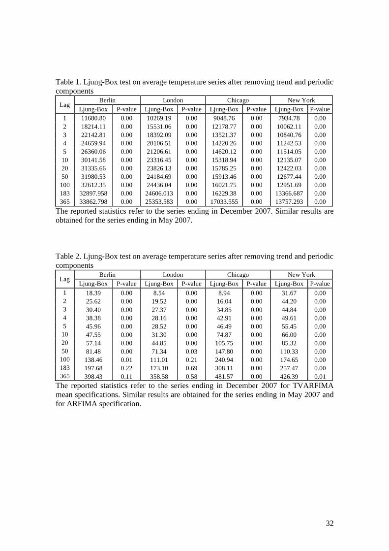
interest, while Table 1 reports the Ljung-Box test for residual correlations over the ty

series in (1), for selected lags.

[TABLE 1]

All series are characterised by a somewhat persistent correlation, which is more evident

in some cases (Berlin and New York). In order to verify if there is a monthly specific

long-term correlation, we computed a monthly variation of the autocorrelation function.

We modified the traditional sample estimator of the autocorrelation function as follows,

(10)

( )( )

( )( )1

2 1

1

1

1

T

t t k Tt k

j Tt

tt

x x I t jM k

k M I t jx I t j

M

ρ−

= +

=

=

∈−= = ∈

∈

∑∑

∑

17

where is the demeaned series of interest (filtered from trend and periodic waves), j is

a given month and I(.) is an indicator function assuming value 1 if observation t belongs

to month j. This approach allowed for identifying changes in persistence across months.

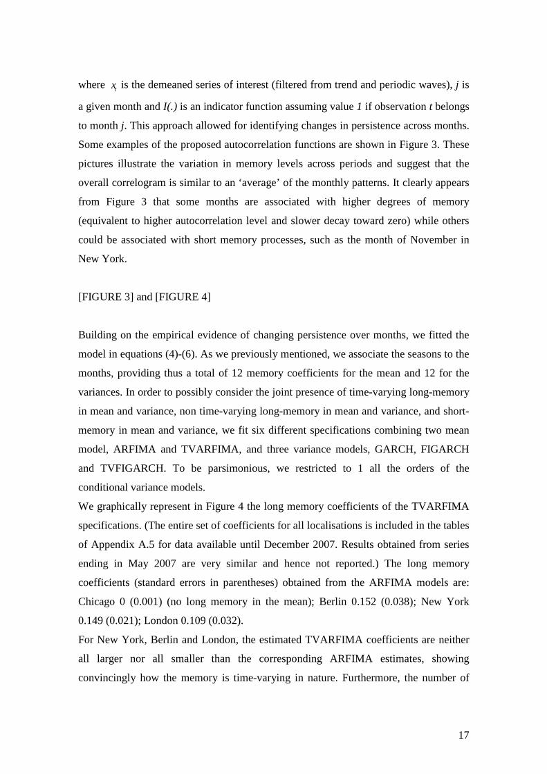
Some examples of the proposed autocorrelation functions are shown in Figure 3. These

pictures illustrate the variation in memory levels across periods and suggest that the

overall correlogram is similar to an ‘average’ of the monthly patterns. It clearly appears

from Figure 3 that some months are associated with higher degrees of memory

(equivalent to higher autocorrelation level and slower decay toward zero) while others

could be associated with short memory processes, such as the month of November in

New York.

[FIGURE 3] and [FIGURE 4]

Building on the empirical evidence of changing persistence over months, we fitted the

model in equations (4)-(6). As we previously mentioned, we associate the seasons to the

months, providing thus a total of 12 memory coefficients for the mean and 12 for the

variances. In order to possibly consider the joint presence of time-varying long-memory

in mean and variance, non time-varying long-memory in mean and variance, and short-

memory in mean and variance, we fit six different specifications combining two mean

model, ARFIMA and TVARFIMA, and three variance models, GARCH, FIGARCH

and TVFIGARCH. To be parsimonious, we restricted to 1 all the orders of the

conditional variance models.

We graphically represent in Figure 4 the long memory coefficients of the TVARFIMA

specifications. (The entire set of coefficients for all localisations is included in the tables

of Appendix A.5 for data available until December 2007. Results obtained from series

ending in May 2007 are very similar and hence not reported.) The long memory

coefficients (standard errors in parentheses) obtained from the ARFIMA models are:

Chicago 0 (0.001) (no long memory in the mean); Berlin 0.152 (0.038); New York

0.149 (0.021); London 0.109 (0.032).

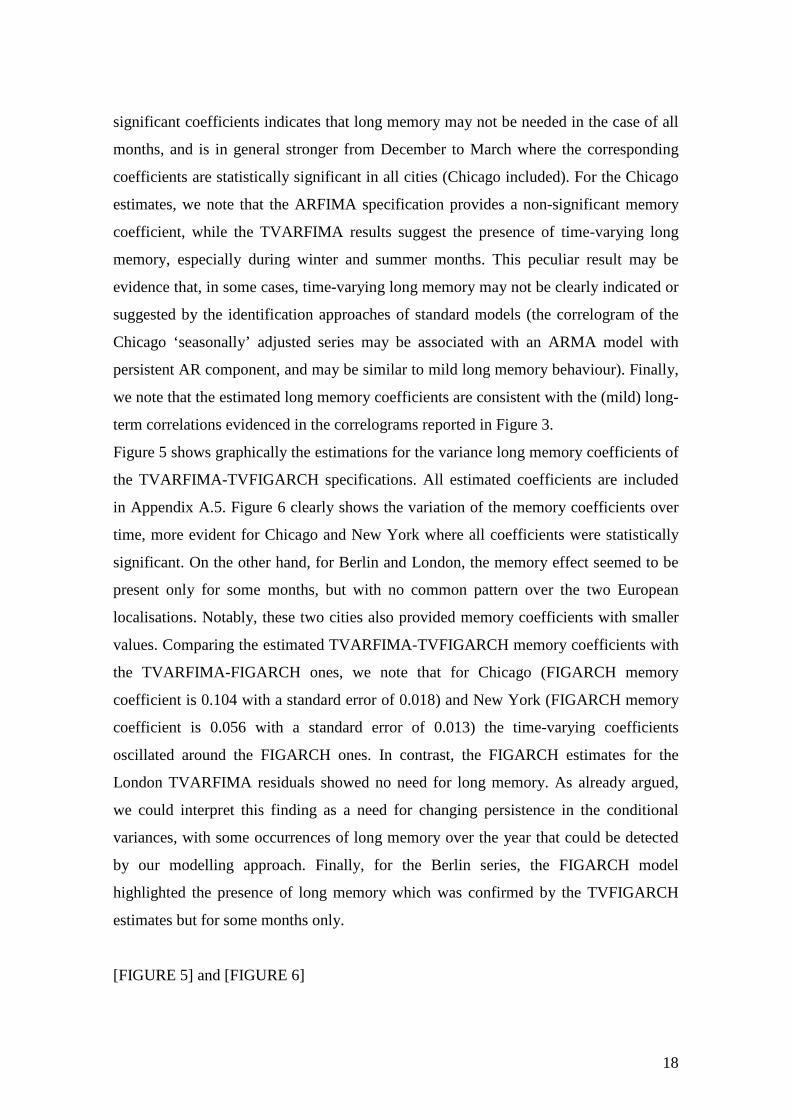
For New York, Berlin and London, the estimated TVARFIMA coefficients are neither

all larger nor all smaller than the corresponding ARFIMA estimates, showing

convincingly how the memory is time-varying in nature. Furthermore, the number of

tx

18

significant coefficients indicates that long memory may not be needed in the case of all

months, and is in general stronger from December to March where the corresponding

coefficients are statistically significant in all cities (Chicago included). For the Chicago

estimates, we note that the ARFIMA specification provides a non-significant memory

coefficient, while the TVARFIMA results suggest the presence of time-varying long

memory, especially during winter and summer months. This peculiar result may be

evidence that, in some cases, time-varying long memory may not be clearly indicated or

suggested by the identification approaches of standard models (the correlogram of the

Chicago ‘seasonally’ adjusted series may be associated with an ARMA model with

persistent AR component, and may be similar to mild long memory behaviour). Finally,

we note that the estimated long memory coefficients are consistent with the (mild) long-

term correlations evidenced in the correlograms reported in Figure 3.

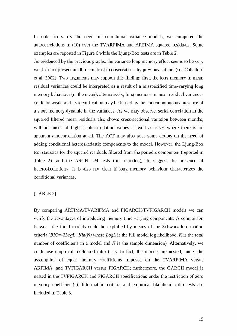
Figure 5 shows graphically the estimations for the variance long memory coefficients of

the TVARFIMA-TVFIGARCH specifications. All estimated coefficients are included

in Appendix A.5. Figure 6 clearly shows the variation of the memory coefficients over

time, more evident for Chicago and New York where all coefficients were statistically

significant. On the other hand, for Berlin and London, the memory effect seemed to be

present only for some months, but with no common pattern over the two European

localisations. Notably, these two cities also provided memory coefficients with smaller

values. Comparing the estimated TVARFIMA-TVFIGARCH memory coefficients with

the TVARFIMA-FIGARCH ones, we note that for Chicago (FIGARCH memory

coefficient is 0.104 with a standard error of 0.018) and New York (FIGARCH memory

coefficient is 0.056 with a standard error of 0.013) the time-varying coefficients

oscillated around the FIGARCH ones. In contrast, the FIGARCH estimates for the

London TVARFIMA residuals showed no need for long memory. As already argued,

we could interpret this finding as a need for changing persistence in the conditional

variances, with some occurrences of long memory over the year that could be detected

by our modelling approach. Finally, for the Berlin series, the FIGARCH model

highlighted the presence of long memory which was confirmed by the TVFIGARCH

estimates but for some months only.

[FIGURE 5] and [FIGURE 6]

19

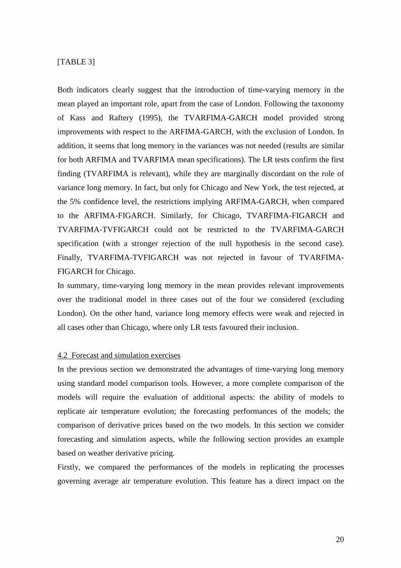
In order to verify the need for conditional variance models, we computed the

autocorrelations in (10) over the TVARFIMA and ARFIMA squared residuals. Some

examples are reported in Figure 6 while the Ljung-Box tests are in Table 2.

As evidenced by the previous graphs, the variance long memory effect seems to be very

weak or not present at all, in contrast to observations by previous authors (see Caballero

et al. 2002). Two arguments may support this finding: first, the long memory in mean

residual variances could be interpreted as a result of a misspecified time-varying long

memory behaviour (in the mean); alternatively, long memory in mean residual variances

could be weak, and its identification may be biased by the contemporaneous presence of

a short memory dynamic in the variances. As we may observe, serial correlation in the

squared filtered mean residuals also shows cross-sectional variation between months,

with instances of higher autocorrelation values as well as cases where there is no

apparent autocorrelation at all. The ACF may also raise some doubts on the need of

adding conditional heteroskedastic components to the model. However, the Ljung-Box

test statistics for the squared residuals filtered from the periodic component (reported in

Table 2), and the ARCH LM tests (not reported), do suggest the presence of

heteroskedasticity. It is also not clear if long memory behaviour characterizes the

conditional variances.

[TABLE 2]

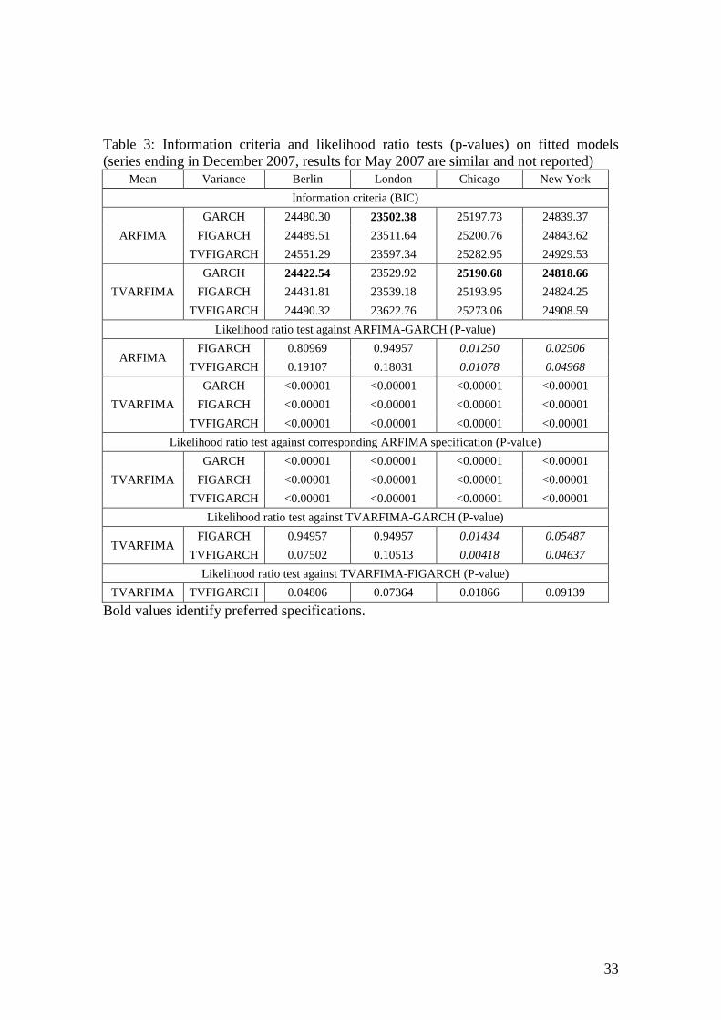
By comparing ARFIMA/TVARIFMA and FIGARCH/TVFIGARCH models we can

verify the advantages of introducing memory time-varying components. A comparison

between the fitted models could be exploited by means of the Schwarz information

criteria (BIC=-2LogL+Kln(N) where LogL is the full model log likelihood, K is the total

number of coefficients in a model and N is the sample dimension). Alternatively, we

could use empirical likelihood ratio tests. In fact, the models are nested, under the

assumption of equal memory coefficients imposed on the TVARFIMA versus

ARFIMA, and TVFIGARCH versus FIGARCH; furthermore, the GARCH model is

nested in the TVFIGARCH and FIGARCH specifications under the restriction of zero

memory coefficient(s). Information criteria and empirical likelihood ratio tests are

included in Table 3.

20

[TABLE 3]

Both indicators clearly suggest that the introduction of time-varying memory in the

mean played an important role, apart from the case of London. Following the taxonomy

of Kass and Raftery (1995), the TVARFIMA-GARCH model provided strong

improvements with respect to the ARFIMA-GARCH, with the exclusion of London. In

addition, it seems that long memory in the variances was not needed (results are similar

for both ARFIMA and TVARFIMA mean specifications). The LR tests confirm the first

finding (TVARFIMA is relevant), while they are marginally discordant on the role of

variance long memory. In fact, but only for Chicago and New York, the test rejected, at

the 5% confidence level, the restrictions implying ARFIMA-GARCH, when compared

to the ARFIMA-FIGARCH. Similarly, for Chicago, TVARFIMA-FIGARCH and

TVARFIMA-TVFIGARCH could not be restricted to the TVARFIMA-GARCH

specification (with a stronger rejection of the null hypothesis in the second case).

Finally, TVARFIMA-TVFIGARCH was not rejected in favour of TVARFIMA-

FIGARCH for Chicago.

In summary, time-varying long memory in the mean provides relevant improvements

over the traditional model in three cases out of the four we considered (excluding

London). On the other hand, variance long memory effects were weak and rejected in

all cases other than Chicago, where only LR tests favoured their inclusion.

4.2 Forecast and simulation exercises

In the previous section we demonstrated the advantages of time-varying long memory

using standard model comparison tools. However, a more complete comparison of the

models will require the evaluation of additional aspects: the ability of models to

replicate air temperature evolution; the forecasting performances of the models; the

comparison of derivative prices based on the two models. In this section we consider

forecasting and simulation aspects, while the following section provides an example

based on weather derivative pricing.

Firstly, we compared the performances of the models in replicating the processes

governing average air temperature evolution. This feature has a direct impact on the

21

pricing process of weather derivatives, which is based on a pure Monte Carlo approach

within the daily modelling we pursue.

We followed the method of Caballero et al. (2002), which was introduced in section 3.2,

and ran a total of N=29000 simulations of monthly average temperature values for each

model and for each localisation. The target periods were set to the months of June 2007

and January 2008. The simulation number allows fixing D=1000 given that the sample

period we use includes 29 years (for June we used N=28000 given that the models were

fitted with data until May 2007). Monthly temperature indices were computed following

the current rules of the CME (see http://rulebook.cme.com).

Table 4 reports the results for New York; results for the other localisations are included

in Appendix A.6. As previously explained, we chose these two specific months in order

to evaluate model abilities in two different seasons of the year, where the memory

degree is very different. We also recall that the models used for the simulation of June

2007 (January 2008) values have been estimated using data until the end of May 2007

(December 2007).

[TABLE 4]

The tables depict the historical mean and standard deviation of the January indices

(HDD index) and the June indices (CDD index for US localisations and the CAT index

for European ones). The approach of Caballero et al. (2002) compared the simulated

mean and standard deviations of the indices, obtained using the fitted models, with the

historical counterparts. For all models the mean differences are very small and not

significantly different from zero according to the reported critical values. As a result,

the models are able to replicate the historical mean of the index Furthermore, it seems

the differences do not follow any particular pattern between American and European

localizations, January against June results and the alternative mean/variance models.

Moving to the evaluation of the simulated standard deviation of the indices, we note

another common pattern: ARFIMA-based simulations provide lower standard

deviations than TVARFIMA-based ones in January, and higher standard deviations than

TVARFIMA-based models in June. In both periods, TVARFIMA specifications provide

standard deviations closer to the historical moments, and, in absolute terms, the

22

difference between ARFIMA and TVARFIMA is smaller in June than in January.

However, if we consider the model evaluation test of Caballero et al. (2002) we note

that the ARFIMA models provide standard deviations not consistent with the historical

standard deviation of the temperature indices. In detail, the tests reject the null

hypothesis of equal moments at the 5% level for New York and at the 10% level for

London. For Chicago, the simulated and historical standard deviations are different only

for ARFIMA-GARCH in January and at the 10% level, while for Berlin ARFIMA

models provide standard deviations different from the historical one in all cases. In

addition, the inclusion of long memory in the variances does not provide any significant

improvement over the standard GARCH model even if, overall, standard deviations are

closer to the historical counterparts.

The choice of January and June may be questionable since we are picking the months

where the monthly-specific long-memory coefficients show the largest deviation from

the yearly long-memory ones. We clearly chose months where the standard ARFIMA-

FIGARCH model and our modification show evidence of different performances. In

other months, the two models are very close one to the other. However, we believe that

time-varying coefficient models are relevant if they over perform the standard

approaches in at least one single seasons, which is what we show. Note also, that our

modelling approach need not to be always the preferred solution. Differently, we are

supporting our method showing that is some cases it is useful.

We also compared models using the simulation approach proposed by Campbell and

Diebold (2005), checking if the in-sample simulations obtained from the models were

able to generate an index density consistent with the true realisation. This additional

check does not depend on a choice of specific months for the comparison and is thus not

affected by the previously evidenced critic on the Caballero et al. (2002) approach. The

model comparison approach of Campbell and Diebold (2005) is based on the

computation of the tail probabilities of the true index realisations over the simulated

index density. If the model is able to replicate in-sample the evolution of an index, the

tail probabilities should be distributed as a uniform density. Therefore, we may assess

the reliability of a model by testing the distribution assumption on the empirical tail

values.

23

[TABLE 5]

Table 5 reports some selected results for Berlin and New York. We observed similar

behaviours for Chicago and London. All models provide empirical tail probabilities,

approximately uniformly distributed, with an overall mild preference for TVARFIMA

specifications (the preference for memory time-varying models is higher during summer

months when CAT/CDD indices are used, in particular for European localisations).

These results partially confirm the previous finding on the impact of the introduction of

time-varying memory behaviour on average temperature modelling (additional results

for all localisations and all models are available from authors on request).

Finally, we provide two simple examples as evidence for the difference between our

modelling strategy and traditional approaches. Figure 7 (Figure 8) reports the Berlin,

January 2008 (New York, June 2007) average temperature values (dotted lines – left

panels) and the evolution of the realised HDD (CDD) index over the days (dotted lines

– right panels). We also included the median (bold lines) and the 1% (outer lines) and

5% (inner lines) obtained from a set of 10000 simulations produced using ARFIMA-

GARCH (upper panels) and TVARFIMA-GARCH (lower panels) models. The

interesting difference is in the width of the simulation quantiles, (wider for Berlin,

narrower for New York) in the TARFIMA-GARCH case. In both cases, the simulated

variances are closer to the historical ones, able to cover more extreme events for Berlin

or to closely follow the mean evolution without unnecessary variability in the New

York case.

4.3 An example on Pricing weather derivatives

In order to present the practical impact of the proposed modelling strategy, we

developed and applied a weather option pricing procedure. All fitted models (combining

ARFIMA/TVARFIMA in mean with the fitted conditional variance components) were

used to estimate the premium value of two weather put options (for June 2007 and

January 2008) for all the previous localisations. The pricing was made at the

hypothetical dates of 31st May 2007 for June options and 31st December 2007 for

January options. The models used to run the Monte Carlo pricing algorithms (based on

24

10000 replications or simulated paths) were estimated using data available until the

pricing day and using the simulation schemes described in Appendix A.2.

Following real market pricing standards of weather options, we increased the derivative

“fair value” obtained from the models by a risk premium calibrated on the payoff

density. We also set the risk-free rate at 4.0% per annum and the tick value used in the

pricing conformed to CME rules. We did not include any additional elements, such as

transaction costs, in the pricing process. Finally, we fixed the strike prices at the same

level for all models. This implies that the different prices provided by the alternative

models will depend on the simulated index mean and standard deviations (at least). In

fact, the simulated paths may induce different simulated index densities. Accordingly,

we decided to price in-the-money put options to demonstrate more clearly the impact of

the differences in standard deviations. Alternatively, we could have sterilized the

differences in the mean pricing under each contract’s at-the-money options, with the

result of having contract price differences related only to moments from the second one

onward. Note also that the introduction of a risk premium is not constant over models

since the simulated index densities may differ. Therefore its introduction may not

correspond to a monotonic transformation of the fair values.

The pricing procedure for weather options may be summarised in these few steps:

1) Compute contract “fair value” as the mean payout from large number (10000) of

simulated index values for the target maturity;

2) Add a risk premium computed as the 4.5% of the 95% percentile of simulated

contract payouts;

3) Discount the price one month back using 4.0% p.a.

Table 6 reports the final prices for June 2007 and January 2008 put options contracts for

New York (see Appendix A.6. for the other localisations). The price differences shown

by the various model comparison approaches induce large variations in option prices,

largely due to different standard deviations (this is an expected outcome given the

importance of variances in the pricing of option contracts). Some price differences are

very large; for example, differences of more than 40% for January (New York) and -

10% for June (London).

[TABLE 6]

25

The previous table shows the impact of modelling strategy on contract prices. These are

an effect of the under- or over-estimation of series variance in the target months. In fact,

the greatest discrepancy between standard models and memory time-varying approaches

is in the variance of simulated temperature indices contracts, as highlighted in the

previous section. Note that the historical variance of air temperature, in all locations, is

much bigger in January than in June. This fact can be captured by the use of a memory

time-varying model. Note that, as in standard ARMA models, the unconditional

variance can be expressed as a function of all model coefficients. As a result, different

mean specifications could lead to different unconditional variances of average

temperature models, to different densities of temperature indices, and thus to different

contract prices.

Furthermore, the application of the traditional ARFIMA-FIGARCH model to the

pricing process leads to the use in all months of a single long memory coefficient,

whether or not the empirical evidence (see Figure 5) suggests some changes in the

autocorrelation structure over time. The misspecification of long memory structure

strongly influences contract prices.

Focusing on the two months we used, January and June, we found that in January

contract prices provided by TVARFIMA specifications were higher than the

corresponding prices obtained from ARFIMA models. From the practitioner’s point of

view, accepting the existence of a single long memory parameter for an entire year

would result in an underestimated variance value for January; this obviously translates

into an underestimation of the final premium value. Analogous but contradictory effects

were observed in June, where all options were overestimated when standard long

memory specifications were used. We conclude by stressing that the use of memory

time-varying models may provide more accurate prices, given that these models are

closer to the real data generating process.

Unfortunately, the contract prices we derived cannot be directly compared to actual

market prices for a number of reasons: the contracts traded at the CME are illiquid and

subject to large price deviations due to the infrequent hedging activities of energy

companies (OTC should be preferred but they are extremely difficult to recover); CME

is considered mainly as a clearing house and not as a true market; providers of weather

contracts are limited (about 20 in 2007 and 2008); the final price charged to the client

26

may include additional fees and the risk premium may be largely increase to cover

additional risk faced by the contract provider (excess volatility in the weather variables,

uncertainty about the forecast and the model, use of a pricing method which is easy to

compute but less accurate).

5. Conclusions

We proposed a modification of the traditional long memory mean and variance

specifications allowing for changes in the memory coefficient over time. In particular,

we allowed the long term correlation to vary in accordance with a step function defined

for the time index. This extension is supported by empirical evidence for changing

degree of memory over months, as observed in average temperature series. The use of

temperature values has a significant impact on the weather derivative market since it

represents the main information source for options and future options (temperature-

based contracts cover about 90% of weather market transactions).

In our empirical study we show the impact of the proposed model, focusing on monthly

variations of persistence in the temperature series. By using model comparisons and

pricing approaches currently available in the literature we evidence that the memory

time-varying component in the mean provides significant improvements both from a

statistical point of view and for the pricing of option contracts. In particular, the contract

prices may be more accurately determined.

The model may be clearly applied also to seasonal variations in the memory level that

could be very relevant in other areas of the statistics and econometric literature, as well

as in the weather derivative pricing framework if applied to different weather variables.

27

References

Alaton, P., B. Djehiche and D. Stillberger, 2002, On modelling and pricing weather derivatives, Applied Mathematical Finance, 9, 1-20

Andersen, T.G. and T. Bollerslev, 1997, Intraday periodicity and volatility persistence in financial markets, Journal of Empirical Finance, 4, 115-158

Andersen, T.G. and T. Bollerslev, 1998, Deutsche mark-dollar volatility: intraday activity patterns, macroeconomic announcements, and longer run dependencies, Journal of Finance, 59, 219-265

Augros, J.C. and M. Moreno, 2002, Les Dérivés Financiers et d’Assurance, Economica

Baillie, R.T., 1996, Long memory processes and fractional integration in econometrics, Journal of Econometrics, 73, 5-59

Baillie, R.T. and T. Bollerslev, 1994, The long memory of the forward premium, Journal of International Money and Finance, 13, 565-571

Baillie, R.T. and S. Chung, 2002, Modeling and forecasting from trend-stationary long memory models with applications to climatology, International Journal of Forecasting, 18, 215-226

Baillie, R.T, T. Bollerslev, and H.O. Mikkelsen, 1996, Fractionally integrated generalized autoregressive conditional heteroskedasticity, Journal of Econometrics, 74, 3-30.

Baillie, R.T., C.F. Chung and M.A. Tieslau, 1996, Analysing inflation by the fractionally integrated ARFIMA-GARCH model, Journal of Applied Econometrics, 11, 23-40

Banks, E., 2002, Weather Risk Management, Markets, Products and Applications, New York, Palgrave.

Beine, M. and S. Laurent, 2003, Central bank interventions and jumps in double long memory models of exchange rates, Journal of Empirical Finance, 10, 641-660

Benth, F.E., 2003, On arbitrage-free pricing of weather derivatives based on fractional Brownian motion, Applied Mathematical Finance, 10, 303-324

Benth, F.E. and J. Saltyté-Benth, 2005, Stochastic modelling of temperature variations with a view toward weather derivatives, Applied Mathematical Finance, 12, 53-85

Beran, J., 1994, Statistics for long-memory processes, Chapman and Hall, New York

Bhardwaj, G. and N.R. Swanson, 2006, An empirical investigation of the usefulness of ARFIMA models for predicting macroeconomic and financial time series, Journal of Econometrics, 131-1, 539-578

Black, F. and M. Scholes, 1973, The pricing of options and corporate liabilities, Journal of Political Economy, 81, 637-659

Bollerslev, T. and J.M. Wooldridge, 1992, Quasi-maximum likelihood estimation and inference in dynamic models with time varying covariances, Econometric Reviews, 11, 143-172

28

Brix, A., S. Jewson and C. Ziehmann, 2002a, Risk Modelling, in Weather Risk Report, Global Reinsurance Review, No 2. 11-15.

Brix, A., S. Jewson and C. Ziehmann, 2002b, Weather derivative modelling and valuation: a statistical perspective, in Climate Risk and the Weather Market, Financial Risks Management with Weather Hedges, ed. Dischel R.S., 127-150

Brix, A., S. Jewson and C. Ziehmann, 2002c, Use of Meteorological Forecasts in Weather Derivative Pricing, in Climate Risk and the Weather Market, Financial Risks Management with Weather Hedges, ed. Dischel R.S., 169-183

Brix, A., S. Jewson and C. Ziehmann , 2005, Weather Derivative Valuation, Cambridge University Press

Brody, D.C., J. Syroka and M. Zervos, 2002, Dynamical pricing of weather derivatives, Quantitative Finance, 2, 189-198

Caballero, R. and S. Jewson, 2002, Multivariate long-memory of daily surface air temperatures and the valuation of weather derivatives, available at SSRN

Caballero, R., S. Jewson and A. Brix, 2002, Long memory in surface air temperature: detection, modelling and application to weather derivative valuation, Climate Research, 21, 127-140

Campbell, S.D. and F.X. Diebold, 2005, Weather forecasting for weather derivatives, Journal of the American Statistical Association, 100-469, 7-16

Cao, M. and J. Wei, 2000, Pricing the weather, Risk Magazine, May, 67-70

Cao, M. and J. Wei, 2003, Weather derivatives valuation and market price of weather risk, Journal of Future Markets, 24, 1065-1090

Cheung, Y., 1993, Long memory in foreign exchange rates, Journal of Business and Economic Statistics, 11, 93-101

Cheung, Y. and K.S. Lai, 1995, A search for long memory in the international stock market returns, Journal of International Money and Finance, 14, 597-615

Clemmons, L., 2002, Introduction to Weather Risk Management, in Weather Risk Management, Markets, Products and Applications, ed. Banks E., 3-4.

Conrad, C. and B.R. Haag, Inequality constraints in the Fractionally Integrated GARCH model, Journal of Financial Econometrics, 4, 413-449

Couchman, J., R. Gounder and J.J. Su, 2006, Long memory properties of real interest rates for 16 countries, Applied Financial Economics Letters, 2, 25-30

Davis, M., 2001, Pricing weather derivatives by marginal value, Quantitative Finance, 1, 1-14

Diebold, F.X. and G.D. Rudebush, 1989, Long memory persistence in aggregate output, Journal of monetary economics, 24, 189-209

Ding, Z., C.W.J. Granger and R.F. Engle, 1993, A long memory property of stock market returns and a new model, Journal of Empirical Finance, 1, 83-106

Dischel, R., 1998, Black-Scholes won’t do, Energy Power and Risk Management Weather Risk Report, 10

29

Dischel, R.S. (Ed.), 2002, Climate risk and the weather market: financial risk management with weather hedges, Risk Publications, London

Doornik, J.A. and M. Ooms, 2004, Inference and forecasting for ARFIMA models with application to US and UK inflation, Studies in Nonlinead Dynamics and Econometrics, 8, 1-23

Dornier, F. and M. Querel, 2000, Caution to the wind, Energy Power and Risk Management Weather Risk Report 8, 30-32

Foster, K., 2003, The trouble with normalisation, Energy and Power Risk Management, No. 7. 22-23.

Franses, P.H. and M. Ooms, 1997, A periodic long-memory model for quarterly UK inflation, International Journal of Forecasting, 13, 117-126

Geman, H. (Ed.), 1999, Insurance and weather derivatives: from exotic options to exotic underlyings, Risk Publications, London

Geweke, J., and S. Porter-Hudak, 1983, The estimation and application of long memory time series models, Journal of Time Series Analysis, 4, 221-238

Gil-Alana, L.A. and J. Toro, 2002, Estimation and testing of ARFIMA models in real exchange rate, International Journal of Finance and Economics, 7, 279-292

Granger, C.W.J., 1980, Long memory relationships and the aggregation of dynamic models, Journal of Econometrics, 14, 227-238

Granger, C.W.J., 1981, Some properties of time series data and their use in econometric model specification, Journal of Econometrics, 16, 121-130

Granger, C.W.J. and R. Joyeux, 1980, An introduction to long memory time series models and fractional differencing, Journal of Time Series Analysis, 1, 15-29

Haldrup, N. and M.O. Nielsen, 2006a, A regime switching long memory model for electricity prices, Journal of Econometrics, 135, 349-376

Haldurp, N. and M.O. Nielsen, 2006b, Directional congestion and regime switching in a long memory model for electricity prices, Studies in nonlinear dynamics and econometrics, 10, 1367-1367

Hamisultane, H., 2006a, Utility-based pricing of the weather derivatives, working paper

Hamisultane, H., 2006b, Pricing the weather derivatives in the presence of long memory in temperatures, working paper

Hassler, U. and J. Wolters, 1995, Long memory in inflation rates: international evidence, Journal of Business and Economic Statistics, 13, 37-45

Henderson, R., 2002, Pricing Weather Risk, in Weather Risk Management, Markets, Products and Applications, ed. Banks E., 167-196.

Hosking, J.R.M., 1981, Fractional differencing, Biometrika, 68, 165-176

Hosking, J.R.M., 1984, Modeling persistence in hydrological time series using fractional differencing, Water Resources Research, 20, 1898-1908

Hui, Y.V. and W.K. Li, 1995, On fractionally differenced periodic processes, Sankhya: The Indian Journal of Statistics, 57(B), 19-31

30

Iglesias, E.M. and G.D.A. Phillips, 2005, Analysing one-month Euro-market interest rates by fractionally integrated models, Applied Financial Economics, 15, 95-106

IPCC, 2007: Summary for Policymakers. In: Climate Change 2007: The Physical Science Basis. Contribution of Working Group I to the Fourth Assessment Report of the Intergovernmental Panel on Climate Change [Solomon, S., D. Qin, M. Manning, Z. Chen, M. Marquis, K.B. Averyt, M.Tignor and H.L. Miller (eds.)]. Cambridge University Press, Cambridge, United Kingdom and New York, NY, USA. – available on http://ipcc-wg1.ucar.edu/wg1/wg1-report.html

Jewson, S., 2004, Weather derivative pricing and the potential of daily temperature modelling, RMS Working Papers.

Jewson, S., 2002, Arbitrage pricing for weather derivatives, Climate Risk and the Weather Market, 314-316

Jewson, S. and R. Caballero, 2002, Seasonality in the statistics of surface air temperature and the pricing of weather derivatives, available at SSRN

Jewson, S. and A. Brix, 2000, Modelling weather derivative portfolios, Environmental finance, 11

Jewson, S. and A. Brix, 2005. Weather derivative valuation. The meteorological, statistical, financial and mathematical foundations, Cambridge University Press

Jewson, S. and M. Zervos, 2003, No-arbitrge pricing of weather derivatives in the presence of a liquid swap market, available at SSRN

Kass, E.K. and A.E. Raftery, 1995, Bayes factors, Journal of the American Statistical Association, 90-430, 773-795

Katz R., 1996, Use of conditional stochastic models to generate climate change scenarios, Climate Change, No. 32, 237-255.

Katz R. and M. Parlange, 1998, An extended version of the Richardson Model for simulating daily weather variables, Journal of Applied Meteorology, No. 39, 610-622.

Koopman, S.J., M. Ooms and M.A. Carnero, 2007, Periodic seasonal Ref-ARFIMA-GARCH models for daily electricity spot prices, Journal of the American Statistical Association, 102-477, 16-27

Ku, A., 2001, Betting on the weather, Global Energy Business, No. 7-8, p 28.

Lo, A.W., 1991 , Long memory in stock market prices, Econometrica, 59, 1279-1313

McWilliams, D., 2004, Does The Weather Affect The European Economy?, Weather Risk Management Association Conference London, 5 November 2004,

Mills, T.C., 1993, Is there a long-term memory in the UK stock returns?, Applied Financial Economics, 3, 303-306

Moreno, M., 2003, Weather derivatives hedging and swap illiquidity, Weather Risk Management Association

Nicholls, M., 2004, Confounding the forecasts, Environmental Finance, No. 10. 5-7.

Nelken I., 2000, Weather Derivatives – Pricing and Hedging, , Super Computer Consulting, Inc. IL. USA , January.

31

Ooms, M. and P.H. Franses, 2001, A seasonal periodic long memory model for monthly river flows Environmental Modelling & Software 16, 559–569

Porter-Hudak, S., 1990, An application of the seasonally fractionally differenced model to the monetary aggregates, Journal of the American Statistical Association, 85, 338-344

Roustant, O., J. Laurent, X. Bay and L. Carraro, 2003, Model risk in the pricing of weather derivatives, working paper

Smith, R.L., 1993, Long-range dependence and global warming, in Barnett, V. and K.F. Turkerman (Eds.), Statistics for the environment, John Wiley & Sons, New York, 141-161

Sowell, F.B., 1992a, Maximum likelihood estimation of stationary univariate fractionally integrated time series models, Journal of Econometrics, 53, 165-188

Sowell, F.B., 1992b, Modeling the long run behaviour with the fractional ARIMA model, Journal of Monetary Economics, 29, 277-302

Taylor, J.W. and R. Buizza, 2006, Density forecasting for weather derivative pricing, International Journal of Forecasting, 22, 29-42

Torro, H., V. Meneu and E. Valor, 2001, Single factor stochastic models with seasonality applied to underlying weather derivative variables, Technical Report 60, European Financial Management Association

Van Lennep, et al., 2004, Weather Derivatives: An Attractive Additional Asset Class, The Journal of Alternative Investments Vol. 7. 7-31.

Weather Risk Management Association Survey 2007, available on WRMA website - http://www.wrma.org

Zeng, L., 2000, Weather derivatives and weather insurance: concept application and analysis, Bulletin of the American Meteorological Society, 81, 2075-2982

32

Table 1. Ljung-Box test on average temperature series after removing trend and periodic components

Lag Berlin London Chicago New York

Ljung-Box P-value Ljung-Box P-value Ljung-Box P-value Ljung-Box P-value 1 11680.80 0.00 10269.19 0.00 9048.76 0.00 7934.78 0.00 2 18214.11 0.00 15531.06 0.00 12178.77 0.00 10062.11 0.00 3 22142.81 0.00 18392.09 0.00 13521.37 0.00 10840.76 0.00 4 24659.94 0.00 20106.51 0.00 14220.26 0.00 11242.53 0.00 5 26360.06 0.00 21206.61 0.00 14620.12 0.00 11514.05 0.00 10 30141.58 0.00 23316.45 0.00 15318.94 0.00 12135.07 0.00 20 31335.66 0.00 23826.13 0.00 15785.25 0.00 12422.03 0.00 50 31980.53 0.00 24184.69 0.00 15913.46 0.00 12677.44 0.00 100 32612.35 0.00 24436.04 0.00 16021.75 0.00 12951.69 0.00 183 32897.958 0.00 24606.013 0.00 16229.38 0.00 13366.687 0.00 365 33862.798 0.00 25353.583 0.00 17033.555 0.00 13757.293 0.00

The reported statistics refer to the series ending in December 2007. Similar results are obtained for the series ending in May 2007. Table 2. Ljung-Box test on average temperature series after removing trend and periodic components

Lag Berlin London Chicago New York

Ljung-Box P-value Ljung-Box P-value Ljung-Box P-value Ljung-Box P-value 1 18.39 0.00 8.54 0.00 8.94 0.00 31.67 0.00 2 25.62 0.00 19.52 0.00 16.04 0.00 44.20 0.00 3 30.40 0.00 27.37 0.00 34.85 0.00 44.84 0.00 4 38.38 0.00 28.16 0.00 42.91 0.00 49.61 0.00 5 45.96 0.00 28.52 0.00 46.49 0.00 55.45 0.00 10 47.55 0.00 31.30 0.00 74.87 0.00 66.00 0.00 20 57.14 0.00 44.85 0.00 105.75 0.00 85.32 0.00 50 81.48 0.00 71.34 0.03 147.80 0.00 110.33 0.00 100 138.46 0.01 111.01 0.21 240.94 0.00 174.65 0.00 183 197.68 0.22 173.10 0.69 308.11 0.00 257.47 0.00 365 398.43 0.11 358.58 0.58 481.57 0.00 426.39 0.01

The reported statistics refer to the series ending in December 2007 for TVARFIMA mean specifications. Similar results are obtained for the series ending in May 2007 and for ARFIMA specification.

33

Table 3: Information criteria and likelihood ratio tests (p-values) on fitted models (series ending in December 2007, results for May 2007 are similar and not reported)

Mean Variance Berlin London Chicago New York

Information criteria (BIC)

ARFIMA

GARCH 24480.30 23502.38 25197.73 24839.37

FIGARCH 24489.51 23511.64 25200.76 24843.62

TVFIGARCH 24551.29 23597.34 25282.95 24929.53

TVARFIMA

GARCH 24422.54 23529.92 25190.68 24818.66

FIGARCH 24431.81 23539.18 25193.95 24824.25

TVFIGARCH 24490.32 23622.76 25273.06 24908.59

Likelihood ratio test against ARFIMA-GARCH (P-value)

ARFIMA FIGARCH 0.80969 0.94957 0.01250 0.02506

TVFIGARCH 0.19107 0.18031 0.01078 0.04968

TVARFIMA

GARCH <0.00001 <0.00001 <0.00001 <0.00001

FIGARCH <0.00001 <0.00001 <0.00001 <0.00001

TVFIGARCH <0.00001 <0.00001 <0.00001 <0.00001

Likelihood ratio test against corresponding ARFIMA specification (P-value)

TVARFIMA

GARCH <0.00001 <0.00001 <0.00001 <0.00001

FIGARCH <0.00001 <0.00001 <0.00001 <0.00001

TVFIGARCH <0.00001 <0.00001 <0.00001 <0.00001

Likelihood ratio test against TVARFIMA-GARCH (P-value)

TVARFIMA FIGARCH 0.94957 0.94957 0.01434 0.05487

TVFIGARCH 0.07502 0.10513 0.00418 0.04637

Likelihood ratio test against TVARFIMA-FIGARCH (P-value)

TVARFIMA TVFIGARCH 0.04806 0.07364 0.01866 0.09139

Bold values identify preferred specifications.

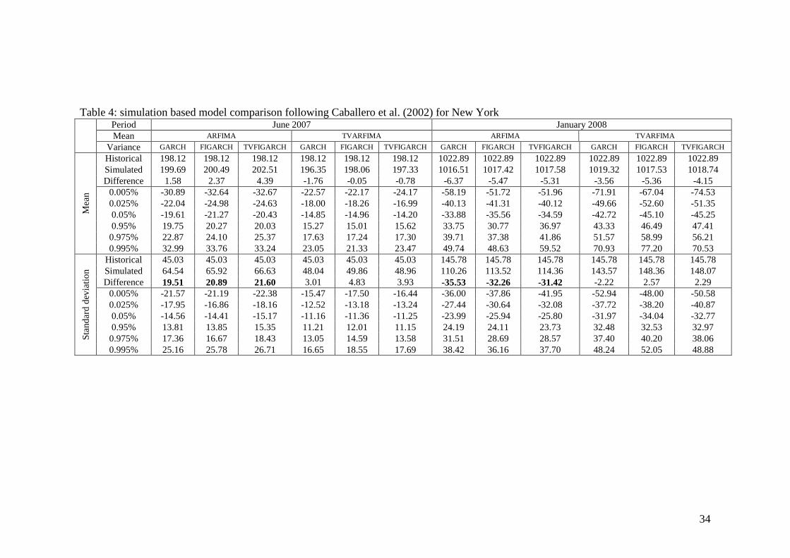
34

Table 4: simulation based model comparison following Caballero et al. (2002) for New York

Period June 2007 January 2008 Mean ARFIMA TVARFIMA ARFIMA TVARFIMA

Variance GARCH FIGARCH TVFIGARCH GARCH FIGARCH TVFIGARCH GARCH FIGARCH TVFIGARCH GARCH FIGARCH TVFIGARCH

Mea

n

Historical 198.12 198.12 198.12 198.12 198.12 198.12 1022.89 1022.89 1022.89 1022.89 1022.89 1022.89 Simulated 199.69 200.49 202.51 196.35 198.06 197.33 1016.51 1017.42 1017.58 1019.32 1017.53 1018.74 Difference 1.58 2.37 4.39 -1.76 -0.05 -0.78 -6.37 -5.47 -5.31 -3.56 -5.36 -4.15

0.005% -30.89 -32.64 -32.67 -22.57 -22.17 -24.17 -58.19 -51.72 -51.96 -71.91 -67.04 -74.53 0.025% -22.04 -24.98 -24.63 -18.00 -18.26 -16.99 -40.13 -41.31 -40.12 -49.66 -52.60 -51.35 0.05% -19.61 -21.27 -20.43 -14.85 -14.96 -14.20 -33.88 -35.56 -34.59 -42.72 -45.10 -45.25 0.95% 19.75 20.27 20.03 15.27 15.01 15.62 33.75 30.77 36.97 43.33 46.49 47.41 0.975% 22.87 24.10 25.37 17.63 17.24 17.30 39.71 37.38 41.86 51.57 58.99 56.21 0.995% 32.99 33.76 33.24 23.05 21.33 23.47 49.74 48.63 59.52 70.93 77.20 70.53

Sta

nd

ard

dev

iatio

n Historical 45.03 45.03 45.03 45.03 45.03 45.03 145.78 145.78 145.78 145.78 145.78 145.78 Simulated 64.54 65.92 66.63 48.04 49.86 48.96 110.26 113.52 114.36 143.57 148.36 148.07 Difference 19.51 20.89 21.60 3.01 4.83 3.93 -35.53 -32.26 -31.42 -2.22 2.57 2.29

0.005% -21.57 -21.19 -22.38 -15.47 -17.50 -16.44 -36.00 -37.86 -41.95 -52.94 -48.00 -50.58 0.025% -17.95 -16.86 -18.16 -12.52 -13.18 -13.24 -27.44 -30.64 -32.08 -37.72 -38.20 -40.87 0.05% -14.56 -14.41 -15.17 -11.16 -11.36 -11.25 -23.99 -25.94 -25.80 -31.97 -34.04 -32.77 0.95% 13.81 13.85 15.35 11.21 12.01 11.15 24.19 24.11 23.73 32.48 32.53 32.97 0.975% 17.36 16.67 18.43 13.05 14.59 13.58 31.51 28.69 28.57 37.40 40.20 38.06 0.995% 25.16 25.78 26.71 16.65 18.55 17.69 38.42 36.16 37.70 48.24 52.05 48.88

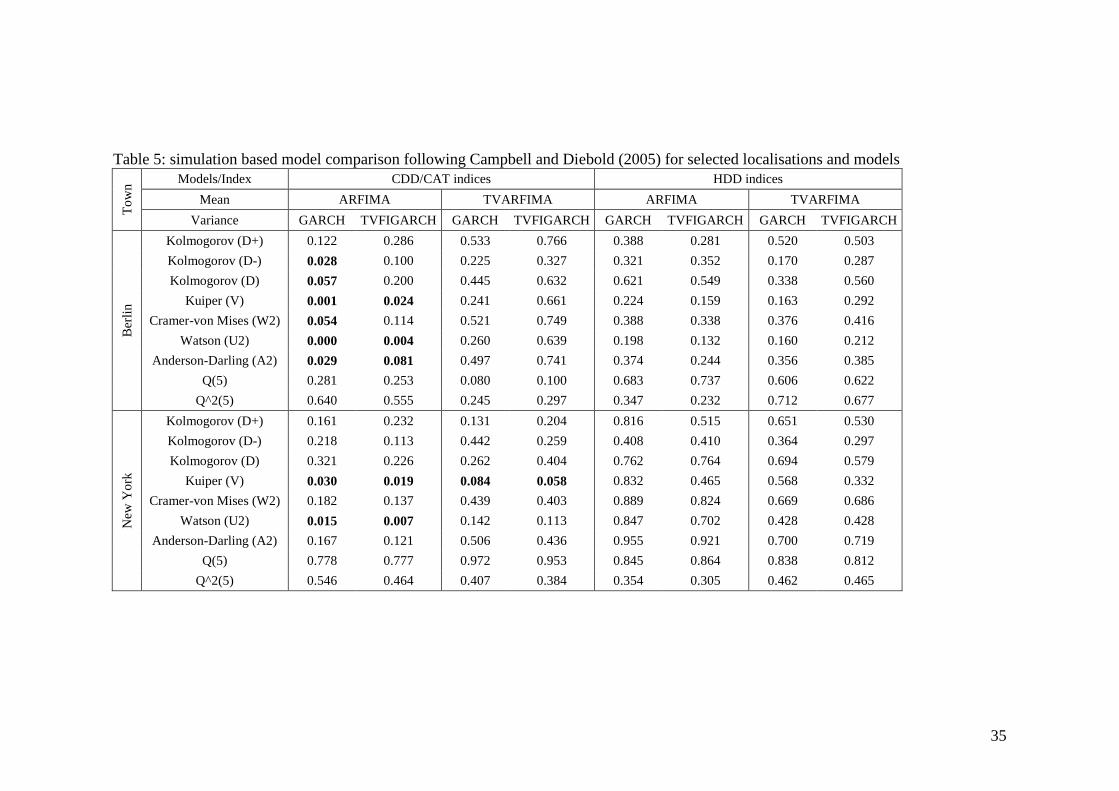
35

Table 5: simulation based model comparison following Campbell and Diebold (2005) for selected localisations and models

To

wn Models/Index CDD/CAT indices HDD indices

Mean ARFIMA TVARFIMA ARFIMA TVARFIMA

Variance GARCH TVFIGARCH GARCH TVFIGARCH GARCH TVFIGARCH GARCH TVFIGARCH

Be

rlin

Kolmogorov (D+) 0.122 0.286 0.533 0.766 0.388 0.281 0.520 0.503

Kolmogorov (D-) 0.028 0.100 0.225 0.327 0.321 0.352 0.170 0.287

Kolmogorov (D) 0.057 0.200 0.445 0.632 0.621 0.549 0.338 0.560

Kuiper (V) 0.001 0.024 0.241 0.661 0.224 0.159 0.163 0.292

Cramer-von Mises (W2) 0.054 0.114 0.521 0.749 0.388 0.338 0.376 0.416

Watson (U2) 0.000 0.004 0.260 0.639 0.198 0.132 0.160 0.212

Anderson-Darling (A2) 0.029 0.081 0.497 0.741 0.374 0.244 0.356 0.385

Q(5) 0.281 0.253 0.080 0.100 0.683 0.737 0.606 0.622

Q^2(5) 0.640 0.555 0.245 0.297 0.347 0.232 0.712 0.677

Ne

w Y

ork

Kolmogorov (D+) 0.161 0.232 0.131 0.204 0.816 0.515 0.651 0.530

Kolmogorov (D-) 0.218 0.113 0.442 0.259 0.408 0.410 0.364 0.297

Kolmogorov (D) 0.321 0.226 0.262 0.404 0.762 0.764 0.694 0.579

Kuiper (V) 0.030 0.019 0.084 0.058 0.832 0.465 0.568 0.332

Cramer-von Mises (W2) 0.182 0.137 0.439 0.403 0.889 0.824 0.669 0.686

Watson (U2) 0.015 0.007 0.142 0.113 0.847 0.702 0.428 0.428

Anderson-Darling (A2) 0.167 0.121 0.506 0.436 0.955 0.921 0.700 0.719

Q(5) 0.778 0.777 0.972 0.953 0.845 0.864 0.838 0.812

Q^2(5) 0.546 0.464 0.407 0.384 0.354 0.305 0.462 0.465

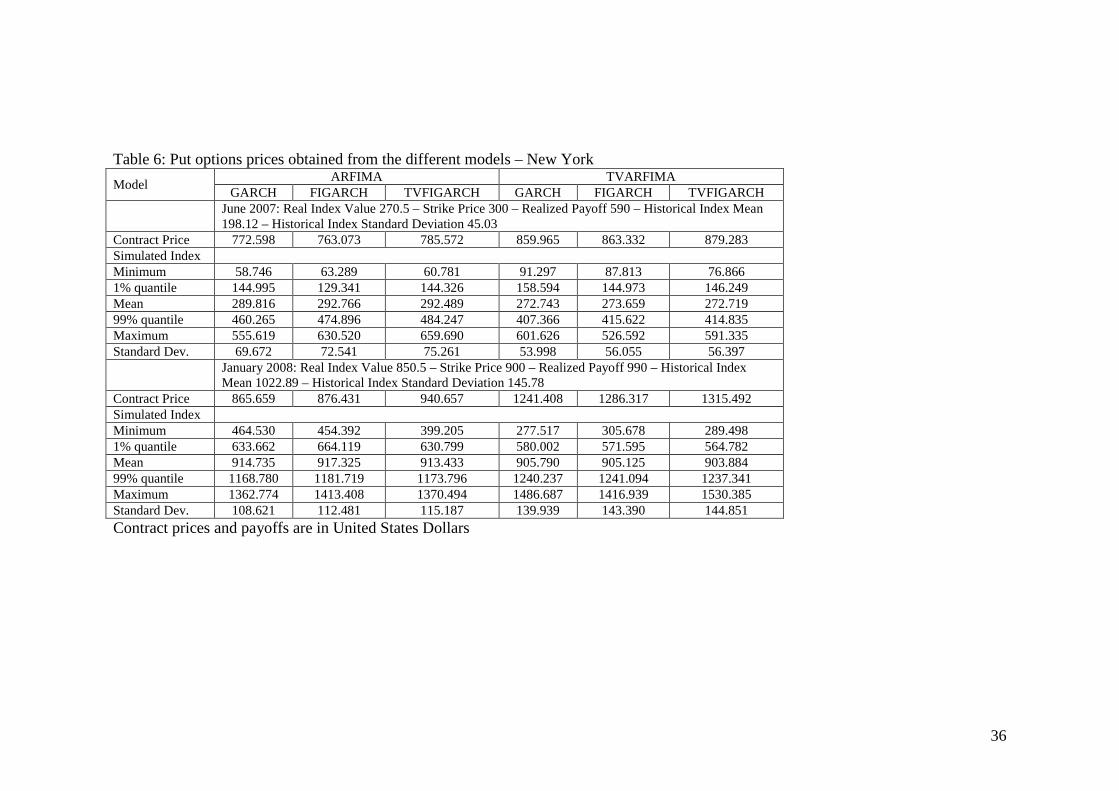
36

Table 6: Put options prices obtained from the different models – New York

Model ARFIMA TVARFIMA

GARCH FIGARCH TVFIGARCH GARCH FIGARCH TVFIGARCH

June 2007: Real Index Value 270.5 – Strike Price 300 – Realized Payoff 590 – Historical Index Mean 198.12 – Historical Index Standard Deviation 45.03

Contract Price 772.598 763.073 785.572 859.965 863.332 879.283 Simulated Index Minimum 58.746 63.289 60.781 91.297 87.813 76.866 1% quantile 144.995 129.341 144.326 158.594 144.973 146.249 Mean 289.816 292.766 292.489 272.743 273.659 272.719 99% quantile 460.265 474.896 484.247 407.366 415.622 414.835 Maximum 555.619 630.520 659.690 601.626 526.592 591.335 Standard Dev. 69.672 72.541 75.261 53.998 56.055 56.397

January 2008: Real Index Value 850.5 – Strike Price 900 – Realized Payoff 990 – Historical Index Mean 1022.89 – Historical Index Standard Deviation 145.78

Contract Price 865.659 876.431 940.657 1241.408 1286.317 1315.492 Simulated Index Minimum 464.530 454.392 399.205 277.517 305.678 289.498 1% quantile 633.662 664.119 630.799 580.002 571.595 564.782 Mean 914.735 917.325 913.433 905.790 905.125 903.884 99% quantile 1168.780 1181.719 1173.796 1240.237 1241.094 1237.341 Maximum 1362.774 1413.408 1370.494 1486.687 1416.939 1530.385 Standard Dev. 108.621 112.481 115.187 139.939 143.390 144.851 Contract prices and payoffs are in United States Dollars

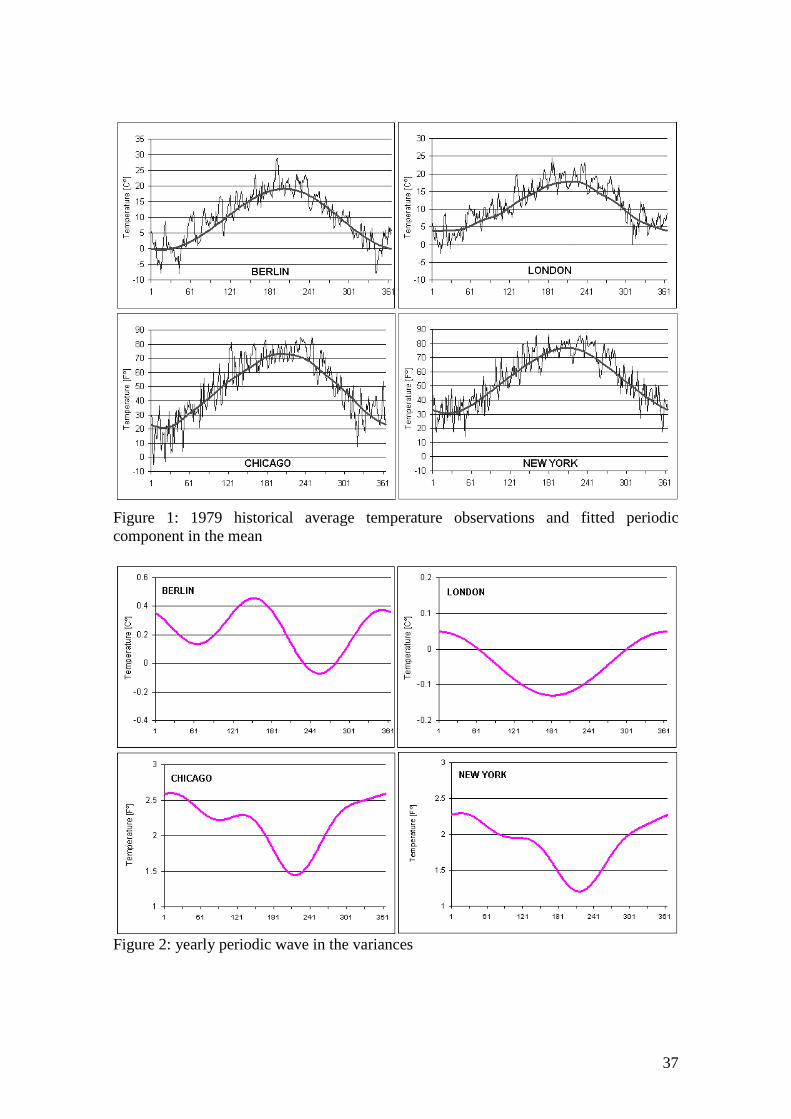
Figure 1: 1979 historical average temperature observations and component in the mean

Figure 2: yearly periodic wave in the variances

1: 1979 historical average temperature observations and

: yearly periodic wave in the variances

37

1: 1979 historical average temperature observations and fitted periodic

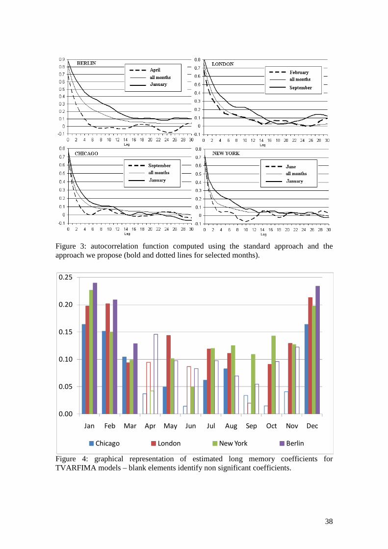
Figure 3: autocorrelation functionapproach we propose (bold and dotted lines for selected months).

Figure 4: graphical representation of estimated long memory coefficients for TVARFIMA models – blank elements identify non significant coefficients.

0.00

0.05

0.10

0.15

0.20

0.25

Jan Feb Mar

Chicago

autocorrelation function computed using the standard approach and the approach we propose (bold and dotted lines for selected months).

graphical representation of estimated long memory coefficients for blank elements identify non significant coefficients.

Apr May Jun Jul Aug Sep Oct

London New York

38

computed using the standard approach and the

graphical representation of estimated long memory coefficients for

blank elements identify non significant coefficients.

Nov Dec

Berlin

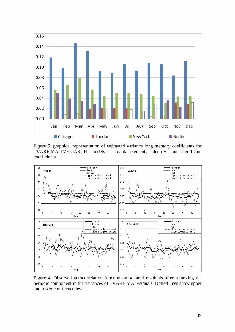
Figure 5: graphical representation of estimated variance long memory coefficients for TVARFIMA- TVFIGARCH models coefficients.

Figure 4. Observed autocorrelation function on squared residualsperiodic component in the variances of TVARFIMA residuals.and lower confidence level.

0.00

0.02

0.04

0.06

0.08

0.10

0.12

0.14

0.16

Jan Feb Mar

Chicago

Figure 5: graphical representation of estimated variance long memory coefficients for TVFIGARCH models – blank elements identify non significant

. Observed autocorrelation function on squared residuals after removing the periodic component in the variances of TVARFIMA residuals. Dotted lines show upper

.

Apr May Jun Jul Aug Sep Oct

London New York

39

Figure 5: graphical representation of estimated variance long memory coefficients for

blank elements identify non significant

after removing the Dotted lines show upper

Nov Dec

Berlin

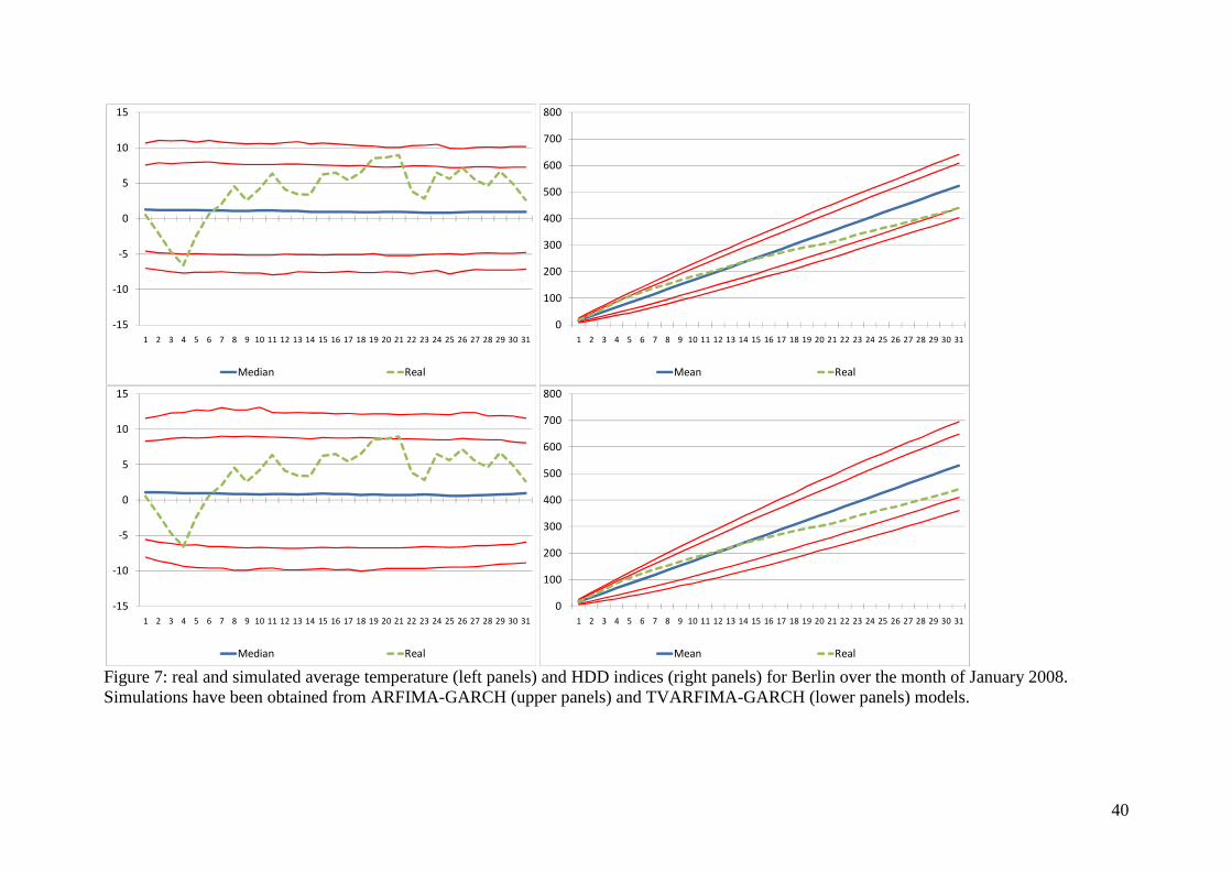
40

Figure 7: real and simulated average temperature (left panels) and HDD indices (right panels) for Berlin over the month of January 2008. Simulations have been obtained from ARFIMA-GARCH (upper panels) and TVARFIMA-GARCH (lower panels) models.

-15

-10

-5

0

5

10

15

1 2 3 4 5 6 7 8 9 10 11 12 13 14 15 16 17 18 19 20 21 22 23 24 25 26 27 28 29 30 31

Median Real

0

100

200

300

400

500

600

700

800

1 2 3 4 5 6 7 8 9 10 11 12 13 14 15 16 17 18 19 20 21 22 23 24 25 26 27 28 29 30 31

Mean Real

-15

-10

-5

0

5

10

15

1 2 3 4 5 6 7 8 9 10 11 12 13 14 15 16 17 18 19 20 21 22 23 24 25 26 27 28 29 30 31

Median Real

0

100

200

300

400

500

600

700

800

1 2 3 4 5 6 7 8 9 10 11 12 13 14 15 16 17 18 19 20 21 22 23 24 25 26 27 28 29 30 31

Mean Real

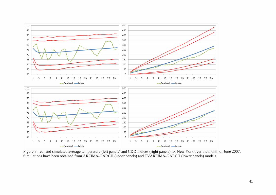
41

Figure 8: real and simulated average temperature (left panels) and CDD indices (right panels) for New York over the month of June 2007. Simulations have been obtained from ARFIMA-GARCH (upper panels) and TVARFIMA-GARCH (lower panels) models.

50

55

60

65

70

75

80

85

90

95

100

1 3 5 7 9 11 13 15 17 19 21 23 25 27 29

Realized Mean

0

50

100

150

200

250

300

350

400

450

500

1 3 5 7 9 11 13 15 17 19 21 23 25 27 29

Realized Mean

50

55

60

65

70

75

80

85

90

95

100

1 3 5 7 9 11 13 15 17 19 21 23 25 27 29

Realized Mean

0

50

100

150

200

250

300

350

400

450

500

1 3 5 7 9 11 13 15 17 19 21 23 25 27 29

Realized Mean

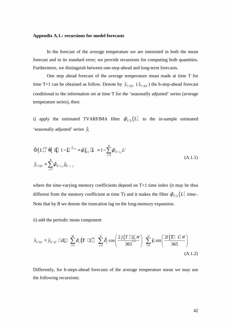
42

Appendix A.1.: recursions for model forecasts

In the forecast of the average temperature we are interested in both the mean

forecast and in its standard error; we provide recursions for computing both quantities.

Furthermore, we distinguish between one-step-ahead and long-term forecasts.

One step ahead forecast of the average temperature mean made at time T for

time T+1 can be obtained as follow. Denote by |ˆT h Ty + ( |ˆT h Tx + ) the h-step-ahead forecast

conditional to the information set at time T for the ‘seasonally adjusted’ series (average

temperature series), then:

i) apply the estimated TVARFIMA filter ( )1ˆT Lψ + to the in-sample estimated

‘seasonally adjusted’ series ˆty

( ) ( ) ( ) ( )1ˆ1

1 1,1

1| 1, 11

ˆ ˆ ˆ ˆ1 1

ˆˆ ˆ

TB

d jT T j

j

B

T T T j T jj

L L L L L

y y

ψ ψ

ψ

+−+ +

=

+ + + −=

Θ Φ − = = −

=

∑

∑ (A.1.1)

where the time-varying memory coefficients depend on T+1 time index (it may be thus

different from the memory coefficient at time T) and it makes the filter ( )1ˆT Lψ + time-.

Note that by B we denote the truncation lag on the long-memory expansion.

ii) add the periodic mean component

(A.1.2)

Differently, for h-steps-ahead forecasts of the average temperature mean we may use

the following recursions:

( ) ( ) ( )1| 1| 0

1 1 1

2 1 2 1ˆˆ ˆ ˆˆ ˆ 1 cos sin365 365

QM Pi

T T T T i j li j l

j T l Tx y T

π πα α δ γ+ +

= = =

+ + = + + + + +

∑ ∑ ∑

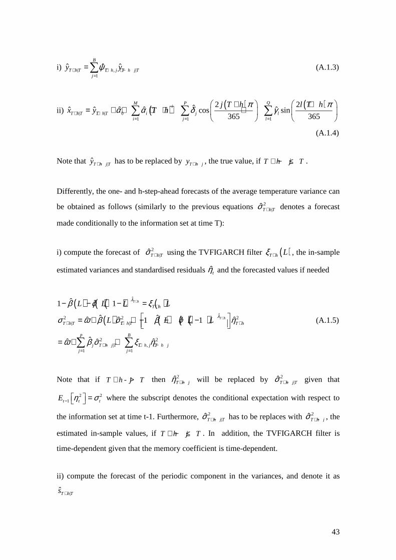
43

i) | , |1

ˆˆ ˆB

T h T T h j T h j Tj

y yψ+ + + −=

=∑ (A.1.3)

ii) ( ) ( ) ( )| | 0

1 1 1

2 2ˆˆ ˆ ˆˆ ˆ cos sin365 365

QM Pi

T h T T hT i j li j l

j T h l T hx y T h

π πα α δ γ+ +

= = =

+ + = + + + + +

∑ ∑ ∑

(A.1.4)

Note that |ˆT h j Ty + − has to be replaced by T h jy + − , the true value, if T h j T+ − ≤ .

Differently, the one- and h-step-ahead forecasts of the average temperature variance can

be obtained as follows (similarly to the previous equations 2|ˆT h Tσ + denotes a forecast

made conditionally to the information set at time T):

i) compute the forecast of 2 |ˆT h Tσ + using the TVFIGARCH filter ( )T h Lξ + , the in-sample

estimated variances and standardised residuals t̂η and the forecasted values if needed

( ) ( ) ( ) ( )( ) ( ) ( ) ( )

ˆ

ˆ2 2 2| |

2 2| ,

1 1

ˆ ˆ1 1

ˆ ˆˆ ˆ ˆˆ 1 1

ˆˆ ˆˆ

T h

T h

T h

T h T T h T T h

p B

j T h j T T h j T h jj j

L L L L

L L L L

λ

λ

β ϕ ξ

σ ω β σ β ϕ η

ω β σ ξ η

+

+

+

+ + +

+ − + + −= =

− − − =

= + + − − −

= + +∑ ∑

(A.1.5)

Note that if -T h j T+ > then 2ˆT h jη + − will be replaced by 2|ˆT h j Tσ + − given that

2 21t t tE η σ− = where the subscript denotes the conditional expectation with respect to

the information set at time t-1. Furthermore, 2|ˆT h j Tσ + − has to be replaces with 2ˆT h jσ + − , the

estimated in-sample values, if T h j T+ − ≤ . In addition, the TVFIGARCH filter is

time-dependent given that the memory coefficient is time-dependent.

ii) compute the forecast of the periodic component in the variances, and denote it as

|ˆT h Ts +

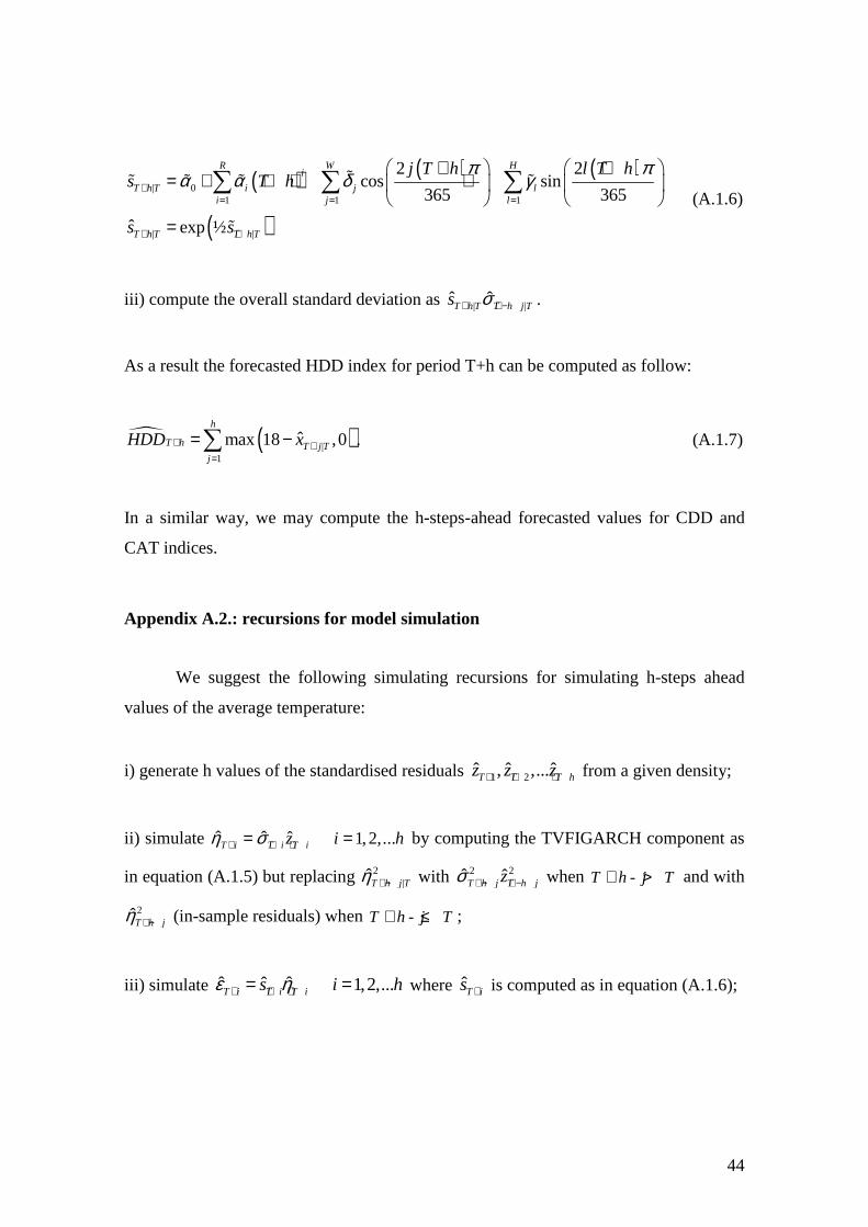
44

( ) ( ) ( )

( )| 0

1 1 1

| |

2 2cos sin

365 365

ˆ exp ½

R W Hi

T h T i j li j l

T h T T h T

j T h l T hs T h

s s

π πα α δ γ+

= = =

+ +

+ + = + + + +

=

∑ ∑ ∑ɶɶ ɶ ɶɶ

ɶ

(A.1.6)

iii) compute the overall standard deviation as | |ˆ ˆT h T T h j Ts σ+ + − .

As a result the forecasted HDD index for period T+h can be computed as follow:

� ( )|1

ˆmax 18 ,0h

T h T j Tj

HDD x+ +=

= −∑ . (A.1.7)

In a similar way, we may compute the h-steps-ahead forecasted values for CDD and

CAT indices.

Appendix A.2.: recursions for model simulation

We suggest the following simulating recursions for simulating h-steps ahead

values of the average temperature:

i) generate h values of the standardised residuals 1 2ˆ ˆ ˆ, ,...T T T hz z z+ + + from a given density;

ii) simulate ˆ ˆ ˆ 1,2,...T i T i T iz i hη σ+ + += = by computing the TVFIGARCH component as

in equation (A.1.5) but replacing 2 |ˆT h j Tη + − with 2 2ˆ ˆT h j T h jzσ + − + − when -T h j T+ > and with

2ˆT h jη + − (in-sample residuals) when -T h j T+ ≤ ;

iii) simulate ˆ ˆˆ 1,2,...T i T i T is i hε η+ + += = where ̂ T is + is computed as in equation (A.1.6);

45

iv) simulate ˆ 1,2,...T iy i h+ = as in equation (A.1.3) replacing |ˆT h Ty + with ˆT hy + (note

that it may represent both in-sample seasonally adjusted values or seasonally adjusted

simulated values);

v) simulate ̂ 1,2,...T ix i h+ = using equation (A.1.4).

Steps i) to v) can be used to simulate one possible realization of the average

temperature. From this realization we may compute a given temperature index. By

repeating many times steps i) to v) we will obtain a large number of temperature indices

which we may use for estimating the density over the interval T+1 to T+h.

In order to provide results consistent with the in-sample realisation of the

underlying process governing the average temperature, the density used in step i) should

be as close as possible to the true one. In general we may fix a density by checking the

distribution of the in-sample residuals t̂z . We may decide to use, say, a normal density

or a more leptokurtic one like the Student density. However, in order to avoid any

possible effect coming from a misspecification of the underlying density, and given that

the time series of average temperature are generally quite long, we suggest simulating

the innovations in i) by resampling with replacement from the in-sample residuals t̂z .

Finally, the previous recursions can be used to simulate entire paths of an average

temperature index without any link to the historical values. In this last case, given the

presence of long-memory, the simulation of a series of length T could benefit for the

inclusion of a presample (that is, the simulated series will have an overall length of

M+T observations, where only the last T will be used).

Appendix A.3. Model comparison following Caballero et al. (2002)

In Caballero et al. (2002), the evaluation of model M follows these steps:

i) compute the historical HDD (or similar) indices for a given period of length T, say the

month of January (the period can be tailored to the contract duration or maturity of

46

interest; it can be the entire year, a specific month or a specific season) over the entire

sample and compute their mean and standard deviation (that is, the set of moments of

interest); assume that the number of historical HDD values is M (continuing the

previous example, HDD for January, in the available sample we have a M values if the

sample length covers about M years) and denote by Hµ and Hσ the historical moments

of the HDD index under evaluation;

ii) simulate a large number of series, N, under model M and compute from each series

one value of the HDD index using last T observations (series should be simulated taking

into account the periodic patterns in order that the last T observations have the same

periodic pattern of the evaluation horizon of the HDD index – as an example, if the

period of interest is the month of January, the last T observation of each simulated series

should be referred to the simulated average temperature of an hypothetical month of

January); compute the mean and the variances of the N simulated HDD values and

denote them by Nµ and Nσ ;

iii) group the N simulated values of the HDD index into D=N/M groups of dimension M

and computed for each group the mean and the variance (the dimension of each group is

equal to the historical observations of the HDD index) which we denote by ,i Sµ and

,i Sσ , with i=1,2,…D;

iv) if D is large, we can use the simulated values to create a confidence interval for the

discrepancies between the overall mean of simulations Nµ and the D means ,i Sµ ; these

confidence interval will take into account the sampling error and will allow testing the

hypothesis that N Hµ µ− = ∆ is large, which can be associated to a model not

completely able to replicate the historical mean of the HDD index (a similar approach

can be used for the variance); the two sided α% confidence interval can be chosen

analysing the differences ,N i S iµ µ− = ∆ and we may denote it as , 12 2

α α ∆ ∆ −

;

47

note that differently from Caballero et al. (2001) we do not assume symmetry of the i∆

density;

v) model M will be rejected if , 12 2

α α ∆∉ ∆ ∆ −

.

In other words, the model comparison approach is based on a bootstrap-like test,

where simulated series can be computed following the recursions presented in appendix

A.2. Given two alternative models, we may prefer the one that has the lower rejection

rate for all moments of interest.

Appendix A.4. Model evaluation following Campbell and Diebold (2001)

In this alternative method, the model comparison approach follows these steps:

i) assume that the interesting contract maturity is the end-of-the-month one (we can use

end-of-the-year or end-of-the-season); then, within the available sample (and also

within the forecast evaluation sample, if available) we have a set of M ‘maturity’ dates

for the contracts, j=1,2,...M; using data up to maturity j-1 (which we assume is the end

of a given month) we simulate many possible patterns of the average temperature index

for maturity j+1 (where 1 is the length of the following maturity period, if months,

length very over time) using the recursions presented in Appendix A.2; given the

simulated average temperature paths we determine the index of interest, the HDD (or

any other temperature-based index);

ii) given the simulated HDD values, we determine its density, and its simulated CDF,

which we denote by FHDD(.);

iii) denote by 1,j jHDD − the realised historical value of the HDD index for the period

between j-1 and j, then we can compute 1, 1,P j j HDD j jx HDD F HDD− − ≤ = , where we

48

assume that the historical value of the HDD index has been extracted from the simulated

density;

iv) iterate steps i) to iii) for all possible periods within the sample (and within the

forecast evaluation sample, if available); we obtain then K values of 1,HDD j jF HDD − ;

if the model we are using is able to simulate reliable or correct HDD densities, then the

values of 1,HDD j jF HDD − for j=1,2...M should be approximately distributed as a

Uniform random variable between 0 and 1, and we can then graph the density of

1,HDD j jF HDD − and test the distributional hypothesis both for the in-sample and out-

of-sample ability of the model.

Given two models, we may prefer the one with a 1,HDD j jF HDD − density closer to the

Uniform(0,1).

Appendix A.5. Estimated coefficients

In this appendix we include the tables reporting the estimated coefficients of the models

we fit on average temperature series. Note we report the results for the model estimated

using series ending in December 2007. The results for series ending in May 2007 are

very similar and not reported for brevity. They can be requested to the authors.

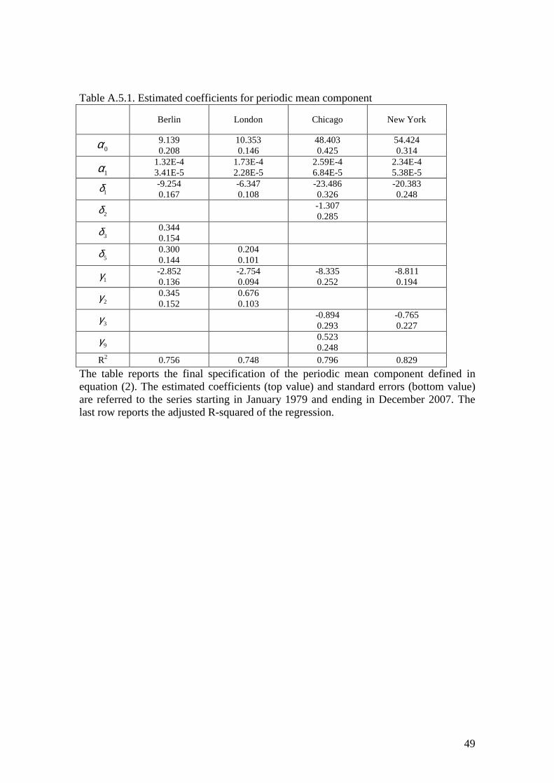
49

Table A.5.1. Estimated coefficients for periodic mean component

Berlin London Chicago New York

0α 9.139 0.208

10.353 0.146

48.403 0.425

54.424 0.314

1α 1.32E-4 3.41E-5

1.73E-4 2.28E-5

2.59E-4 6.84E-5

2.34E-4 5.38E-5

1δ -9.254 0.167

-6.347 0.108

-23.486 0.326

-20.383 0.248

2δ -1.307 0.285

3δ 0.344 0.154

5δ 0.300 0.144

0.204 0.101

1γ -2.852 0.136

-2.754 0.094

-8.335 0.252

-8.811 0.194

2γ 0.345 0.152

0.676 0.103

3γ -0.894 0.293

-0.765 0.227

9γ 0.523 0.248

R2 0.756 0.748 0.796 0.829

The table reports the final specification of the periodic mean component defined in equation (2). The estimated coefficients (top value) and standard errors (bottom value) are referred to the series starting in January 1979 and ending in December 2007. The last row reports the adjusted R-squared of the regression.

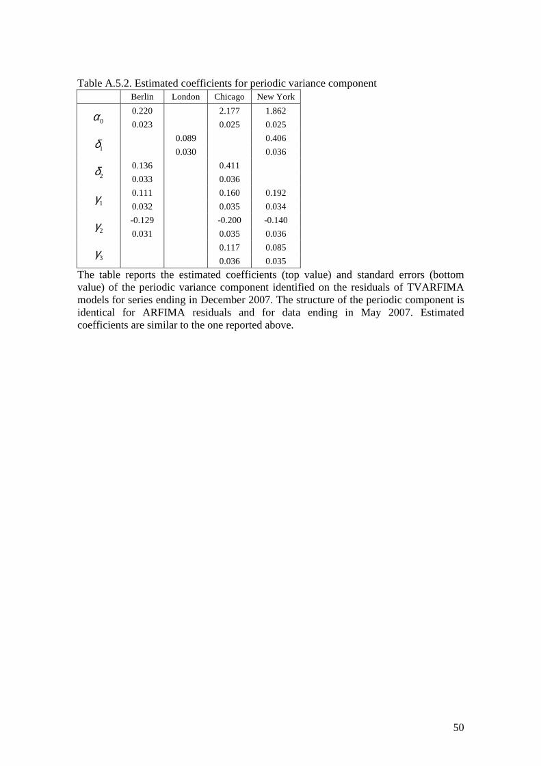
50

Table A.5.2. Estimated coefficients for periodic variance component

Berlin London Chicago New York

0α 0.220

2.177 1.862

0.023

0.025 0.025

1δ 0.089

0.406

0.030

0.036

2δ 0.136

0.411

0.033

0.036

1γ 0.111

0.160 0.192

0.032

0.035 0.034

2γ -0.129

-0.200 -0.140

0.031

0.035 0.036

3γ 0.117 0.085

0.036 0.035

The table reports the estimated coefficients (top value) and standard errors (bottom value) of the periodic variance component identified on the residuals of TVARFIMA models for series ending in December 2007. The structure of the periodic component is identical for ARFIMA residuals and for data ending in May 2007. Estimated coefficients are similar to the one reported above.

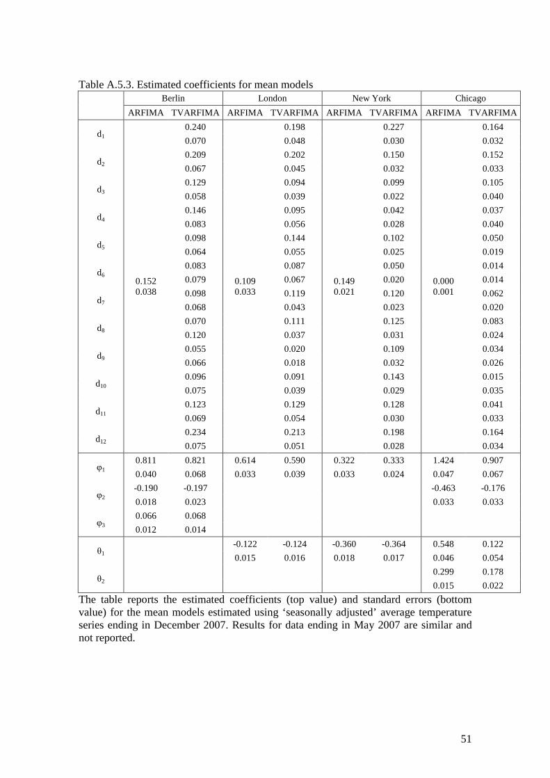
51

Table A.5.3. Estimated coefficients for mean models

Berlin London New York Chicago

ARFIMA TVARFIMA ARFIMA TVARFIMA ARFIMA TVARFIMA ARFIMA TVARFIMA

d1

0.152 0.038

0.240

0.109 0.033

0.198

0.149 0.021

0.227

0.000 0.001

0.164

0.070 0.048 0.030 0.032

d2 0.209 0.202 0.150 0.152

0.067 0.045 0.032 0.033

d3 0.129 0.094 0.099 0.105

0.058 0.039 0.022 0.040

d4 0.146 0.095 0.042 0.037

0.083 0.056 0.028 0.040

d5 0.098 0.144 0.102 0.050

0.064 0.055 0.025 0.019

d6 0.083 0.087 0.050 0.014

0.079 0.067 0.020 0.014

d7 0.098 0.119 0.120 0.062

0.068 0.043 0.023 0.020

d8 0.070 0.111 0.125 0.083

0.120 0.037 0.031 0.024

d9 0.055 0.020 0.109 0.034

0.066 0.018 0.032 0.026

d10 0.096 0.091 0.143 0.015

0.075 0.039 0.029 0.035

d11 0.123 0.129 0.128 0.041

0.069 0.054 0.030 0.033

d12 0.234 0.213 0.198 0.164

0.075 0.051 0.028 0.034

φ1 0.811 0.821 0.614 0.590 0.322 0.333 1.424 0.907

0.040 0.068 0.033 0.039 0.033 0.024 0.047 0.067

φ2 -0.190 -0.197

-0.463 -0.176

0.018 0.023

0.033 0.033

φ3 0.066 0.068

0.012 0.014

θ1 -0.122 -0.124 -0.360 -0.364 0.548 0.122

0.015 0.016 0.018 0.017 0.046 0.054

θ2 0.299 0.178

0.015 0.022

The table reports the estimated coefficients (top value) and standard errors (bottom value) for the mean models estimated using ‘seasonally adjusted’ average temperature series ending in December 2007. Results for data ending in May 2007 are similar and not reported.

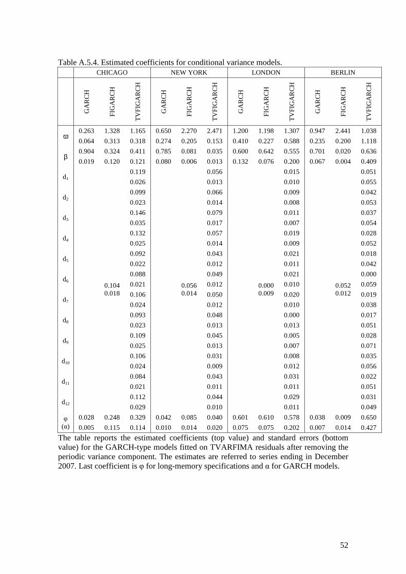
52

Table A.5.4. Estimated coefficients for conditional variance models.

CHICAGO NEW YORK LONDON BERLIN

GA

RC

H

FIG

AR

CH

TV

FIG

AR

CH

GA

RC

H

FIG

AR

CH

TV

FIG

AR

CH

GA

RC

H

FIG

AR

CH

TV

FIG

AR

CH

GA

RC

H

FIG

AR

CH

TV

FIG

AR

CH

ω 0.263 1.328 1.165 0.650 2.270 2.471 1.200 1.198 1.307 0.947 2.441 1.038

0.064 0.313 0.318 0.274 0.205 0.153 0.410 0.227 0.588 0.235 0.200 1.118

β 0.904 0.324 0.411 0.785 0.081 0.035 0.600 0.642 0.555 0.701 0.020 0.636

0.019 0.120 0.121 0.080 0.006 0.013 0.132 0.076 0.200 0.067 0.004 0.409

d1

0.104 0.018

0.119

0.056 0.014

0.056

0.000 0.009

0.015

0.052 0.012

0.051

0.026

0.013

0.010

0.055

d2 0.099

0.066

0.009

0.042

0.023

0.014

0.008

0.053

d3 0.146

0.079

0.011

0.037

0.035

0.017

0.007

0.054

d4 0.132

0.057

0.019

0.028

0.025

0.014

0.009

0.052

d5 0.092

0.043

0.021

0.018

0.022

0.012

0.011

0.042

d6 0.088

0.049

0.021

0.000

0.021

0.012

0.010

0.059

d7 0.106

0.050

0.020

0.019

0.024

0.012

0.010

0.038

d8 0.093

0.048

0.000

0.017

0.023

0.013

0.013

0.051

d9 0.109

0.045

0.005

0.028

0.025

0.013

0.007

0.071

d10 0.106

0.031

0.008

0.035

0.024

0.009

0.012

0.056

d11 0.084

0.043

0.031

0.022

0.021

0.011

0.011

0.051

d12 0.112

0.044

0.029

0.031

0.029

0.010

0.011

0.049

φ (α)

0.028 0.248 0.329 0.042 0.085 0.040 0.601 0.610 0.578 0.038 0.009 0.650

0.005 0.115 0.114 0.010 0.014 0.020 0.075 0.075 0.202 0.007 0.014 0.427

The table reports the estimated coefficients (top value) and standard errors (bottom value) for the GARCH-type models fitted on TVARFIMA residuals after removing the periodic variance component. The estimates are referred to series ending in December 2007. Last coefficient is φ for long-memory specifications and α for GARCH models.

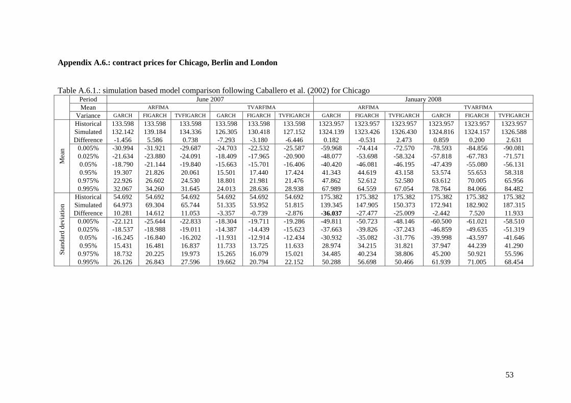
53

Appendix A.6.: contract prices for Chicago, Berlin and London Table A.6.1.: simulation based model comparison following Caballero et al. (2002) for Chicago Period June 2007 January 2008

Mean ARFIMA TVARFIMA ARFIMA TVARFIMA

Variance GARCH FIGARCH TVFIGARCH GARCH FIGARCH TVFIGARCH GARCH FIGARCH TVFIGARCH GARCH FIGARCH TVFIGARCH

Me

an

Historical 133.598 133.598 133.598 133.598 133.598 133.598 1323.957 1323.957 1323.957 1323.957 1323.957 1323.957 Simulated 132.142 139.184 134.336 126.305 130.418 127.152 1324.139 1323.426 1326.430 1324.816 1324.157 1326.588 Difference -1.456 5.586 0.738 -7.293 -3.180 -6.446 0.182 -0.531 2.473 0.859 0.200 2.631

0.005% -30.994 -31.921 -29.687 -24.703 -22.532 -25.587 -59.968 -74.414 -72.570 -78.593 -84.856 -90.081 0.025% -21.634 -23.880 -24.091 -18.409 -17.965 -20.900 -48.077 -53.698 -58.324 -57.818 -67.783 -71.571 0.05% -18.790 -21.144 -19.840 -15.663 -15.701 -16.406 -40.420 -46.081 -46.195 -47.439 -55.080 -56.131 0.95% 19.307 21.826 20.061 15.501 17.440 17.424 41.343 44.619 43.158 53.574 55.653 58.318 0.975% 22.926 26.602 24.530 18.801 21.981 21.476 47.862 52.612 52.580 63.612 70.005 65.956 0.995% 32.067 34.260 31.645 24.013 28.636 28.938 67.989 64.559 67.054 78.764 84.066 84.482

Sta

nd

ard

dev

iatio

n Historical 54.692 54.692 54.692 54.692 54.692 54.692 175.382 175.382 175.382 175.382 175.382 175.382 Simulated 64.973 69.304 65.744 51.335 53.952 51.815 139.345 147.905 150.373 172.941 182.902 187.315 Difference 10.281 14.612 11.053 -3.357 -0.739 -2.876 -36.037 -27.477 -25.009 -2.442 7.520 11.933

0.005% -22.121 -25.644 -22.833 -18.304 -19.711 -19.286 -49.811 -50.723 -48.146 -60.500 -61.021 -58.510 0.025% -18.537 -18.988 -19.011 -14.387 -14.439 -15.623 -37.663 -39.826 -37.243 -46.859 -49.635 -51.319 0.05% -16.245 -16.840 -16.202 -11.931 -12.914 -12.434 -30.932 -35.082 -31.776 -39.998 -43.597 -41.646 0.95% 15.431 16.481 16.837 11.733 13.725 11.633 28.974 34.215 31.821 37.947 44.239 41.290 0.975% 18.732 20.225 19.973 15.265 16.079 15.021 34.485 40.234 38.806 45.200 50.921 55.596 0.995% 26.126 26.843 27.596 19.662 20.794 22.152 50.288 56.698 50.466 61.939 71.005 68.454

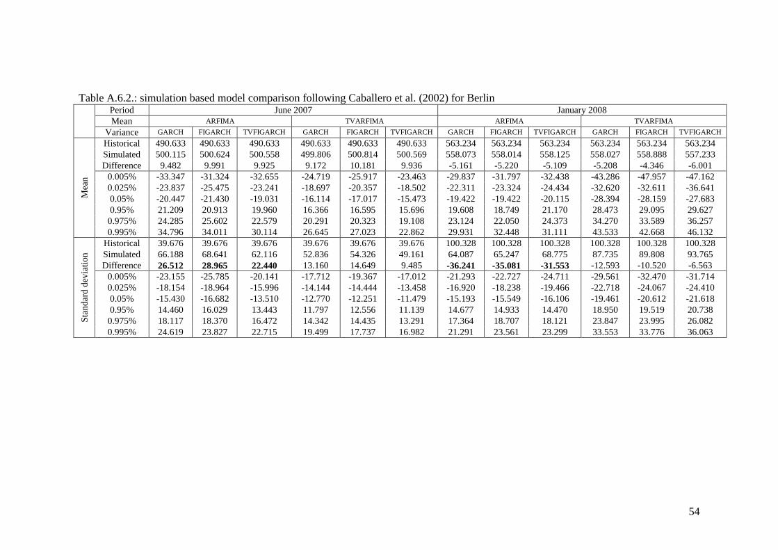
54

Table A.6.2.: simulation based model comparison following Caballero et al. (2002) for Berlin Period June 2007 January 2008

Mean ARFIMA TVARFIMA ARFIMA TVARFIMA

Variance GARCH FIGARCH TVFIGARCH GARCH FIGARCH TVFIGARCH GARCH FIGARCH TVFIGARCH GARCH FIGARCH TVFIGARCH

Mea

n

Historical 490.633 490.633 490.633 490.633 490.633 490.633 563.234 563.234 563.234 563.234 563.234 563.234 Simulated 500.115 500.624 500.558 499.806 500.814 500.569 558.073 558.014 558.125 558.027 558.888 557.233 Difference 9.482 9.991 9.925 9.172 10.181 9.936 -5.161 -5.220 -5.109 -5.208 -4.346 -6.001

0.005% -33.347 -31.324 -32.655 -24.719 -25.917 -23.463 -29.837 -31.797 -32.438 -43.286 -47.957 -47.162 0.025% -23.837 -25.475 -23.241 -18.697 -20.357 -18.502 -22.311 -23.324 -24.434 -32.620 -32.611 -36.641 0.05% -20.447 -21.430 -19.031 -16.114 -17.017 -15.473 -19.422 -19.422 -20.115 -28.394 -28.159 -27.683 0.95% 21.209 20.913 19.960 16.366 16.595 15.696 19.608 18.749 21.170 28.473 29.095 29.627 0.975% 24.285 25.602 22.579 20.291 20.323 19.108 23.124 22.050 24.373 34.270 33.589 36.257 0.995% 34.796 34.011 30.114 26.645 27.023 22.862 29.931 32.448 31.111 43.533 42.668 46.132

Sta

nd

ard

dev

iatio

n Historical 39.676 39.676 39.676 39.676 39.676 39.676 100.328 100.328 100.328 100.328 100.328 100.328 Simulated 66.188 68.641 62.116 52.836 54.326 49.161 64.087 65.247 68.775 87.735 89.808 93.765 Difference 26.512 28.965 22.440 13.160 14.649 9.485 -36.241 -35.081 -31.553 -12.593 -10.520 -6.563

0.005% -23.155 -25.785 -20.141 -17.712 -19.367 -17.012 -21.293 -22.727 -24.711 -29.561 -32.470 -31.714 0.025% -18.154 -18.964 -15.996 -14.144 -14.444 -13.458 -16.920 -18.238 -19.466 -22.718 -24.067 -24.410 0.05% -15.430 -16.682 -13.510 -12.770 -12.251 -11.479 -15.193 -15.549 -16.106 -19.461 -20.612 -21.618 0.95% 14.460 16.029 13.443 11.797 12.556 11.139 14.677 14.933 14.470 18.950 19.519 20.738 0.975% 18.117 18.370 16.472 14.342 14.435 13.291 17.364 18.707 18.121 23.847 23.995 26.082 0.995% 24.619 23.827 22.715 19.499 17.737 16.982 21.291 23.561 23.299 33.553 33.776 36.063

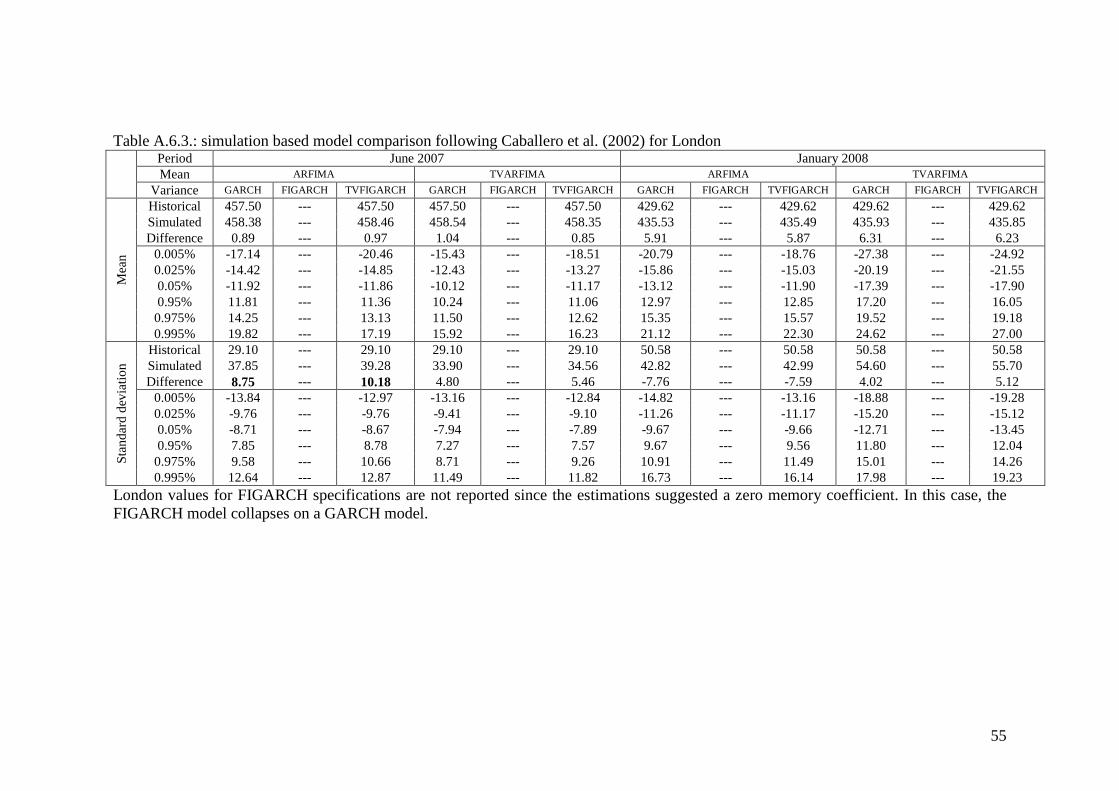
55

Table A.6.3.: simulation based model comparison following Caballero et al. (2002) for London Period June 2007 January 2008

Mean ARFIMA TVARFIMA ARFIMA TVARFIMA

Variance GARCH FIGARCH TVFIGARCH GARCH FIGARCH TVFIGARCH GARCH FIGARCH TVFIGARCH GARCH FIGARCH TVFIGARCH

Mea

n

Historical 457.50 --- 457.50 457.50 --- 457.50 429.62 --- 429.62 429.62 --- 429.62 Simulated 458.38 --- 458.46 458.54 --- 458.35 435.53 --- 435.49 435.93 --- 435.85 Difference 0.89 --- 0.97 1.04 --- 0.85 5.91 --- 5.87 6.31 --- 6.23

0.005% -17.14 --- -20.46 -15.43 --- -18.51 -20.79 --- -18.76 -27.38 --- -24.92 0.025% -14.42 --- -14.85 -12.43 --- -13.27 -15.86 --- -15.03 -20.19 --- -21.55 0.05% -11.92 --- -11.86 -10.12 --- -11.17 -13.12 --- -11.90 -17.39 --- -17.90 0.95% 11.81 --- 11.36 10.24 --- 11.06 12.97 --- 12.85 17.20 --- 16.05 0.975% 14.25 --- 13.13 11.50 --- 12.62 15.35 --- 15.57 19.52 --- 19.18 0.995% 19.82 --- 17.19 15.92 --- 16.23 21.12 --- 22.30 24.62 --- 27.00

Sta

nd

ard

dev

iatio

n Historical 29.10 --- 29.10 29.10 --- 29.10 50.58 --- 50.58 50.58 --- 50.58 Simulated 37.85 --- 39.28 33.90 --- 34.56 42.82 --- 42.99 54.60 --- 55.70 Difference 8.75 --- 10.18 4.80 --- 5.46 -7.76 --- -7.59 4.02 --- 5.12

0.005% -13.84 --- -12.97 -13.16 --- -12.84 -14.82 --- -13.16 -18.88 --- -19.28 0.025% -9.76 --- -9.76 -9.41 --- -9.10 -11.26 --- -11.17 -15.20 --- -15.12 0.05% -8.71 --- -8.67 -7.94 --- -7.89 -9.67 --- -9.66 -12.71 --- -13.45 0.95% 7.85 --- 8.78 7.27 --- 7.57 9.67 --- 9.56 11.80 --- 12.04 0.975% 9.58 --- 10.66 8.71 --- 9.26 10.91 --- 11.49 15.01 --- 14.26 0.995% 12.64 --- 12.87 11.49 --- 11.82 16.73 --- 16.14 17.98 --- 19.23

London values for FIGARCH specifications are not reported since the estimations suggested a zero memory coefficient. In this case, the FIGARCH model collapses on a GARCH model.

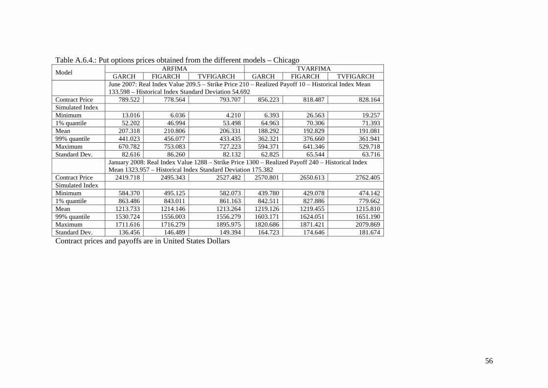
56

Table A.6.4.: Put options prices obtained from the different models – Chicago

Model ARFIMA TVARFIMA

GARCH FIGARCH TVFIGARCH GARCH FIGARCH TVFIGARCH

June 2007: Real Index Value 209.5 – Strike Price 210 – Realized Payoff 10 – Historical Index Mean 133.598 – Historical Index Standard Deviation 54.692

Contract Price 789.522 778.564 793.707 856.223 818.487 828.164 Simulated Index Minimum 13.016 6.036 4.210 6.393 26.563 19.257 1% quantile 52.202 46.994 53.498 64.963 70.306 71.393 Mean 207.318 210.806 206.331 188.292 192.829 191.081 99% quantile 441.023 456.077 433.435 362.321 376.660 361.941 Maximum 670.782 753.083 727.223 594.371 641.346 529.718 Standard Dev. 82.616 86.260 82.132 62.825 65.544 63.716

January 2008: Real Index Value 1288 – Strike Price 1300 – Realized Payoff 240 – Historical Index Mean 1323.957 – Historical Index Standard Deviation 175.382

Contract Price 2419.718 2495.343 2527.482 2570.801 2650.613 2762.405 Simulated Index Minimum 584.370 495.125 582.073 439.780 429.078 474.142 1% quantile 863.486 843.011 861.163 842.511 827.886 779.662 Mean 1213.733 1214.146 1213.264 1219.126 1219.455 1215.810 99% quantile 1530.724 1556.003 1556.279 1603.171 1624.051 1651.190 Maximum 1711.616 1716.279 1895.975 1820.686 1871.421 2079.869 Standard Dev. 136.456 146.489 149.394 164.723 174.646 181.674 Contract prices and payoffs are in United States Dollars

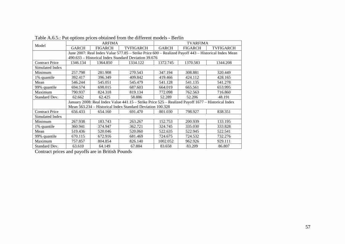
57

Table A.6.5.: Put options prices obtained from the different models - Berlin

Model ARFIMA TVARFIMA

GARCH FIGARCH TVFIGARCH GARCH FIGARCH TVFIGARCH

June 2007: Real Index Value 577.85 – Strike Price 600 – Realized Payoff 443 – Historical Index Mean 490.633 – Historical Index Standard Deviation 39.676

Contract Price 1346.134 1364.850 1334.122 1372.745 1370.583 1344.208 Simulated Index Minimum 257.798 281.908 270.543 347.194 308.881 320.449 1% quantile 392.417 396.349 409.842 419.466 424.112 428.165 Mean 546.244 545.051 545.479 541.128 541.135 541.278 99% quantile 694.574 698.015 687.603 664.019 665.561 653.995 Maximum 790.937 824.318 819.134 772.098 762.563 716.860 Standard Dev. 62.662 62.425 58.886 52.289 52.206 48.191

January 2008: Real Index Value 441.15 – Strike Price 525 – Realized Payoff 1677 – Historical Index Mean 563.234 – Historical Index Standard Deviation 100.328

Contract Price 656.433 654.160 691.470 801.030 798.927 838.351 Simulated Index Minimum 267.938 183.743 263.267 152.753 200.939 133.195 1% quantile 360.941 374.947 362.721 324.745 335.030 333.828 Mean 519.436 520.046 520.060 522.635 522.945 522.541 99% quantile 670.115 672.916 681.469 724.675 724.532 732.276 Maximum 757.857 804.854 826.140 1002.052 962.926 929.111 Standard Dev. 63.610 64.149 67.884 83.658 83.209 86.807 Contract prices and payoffs are in British Pounds

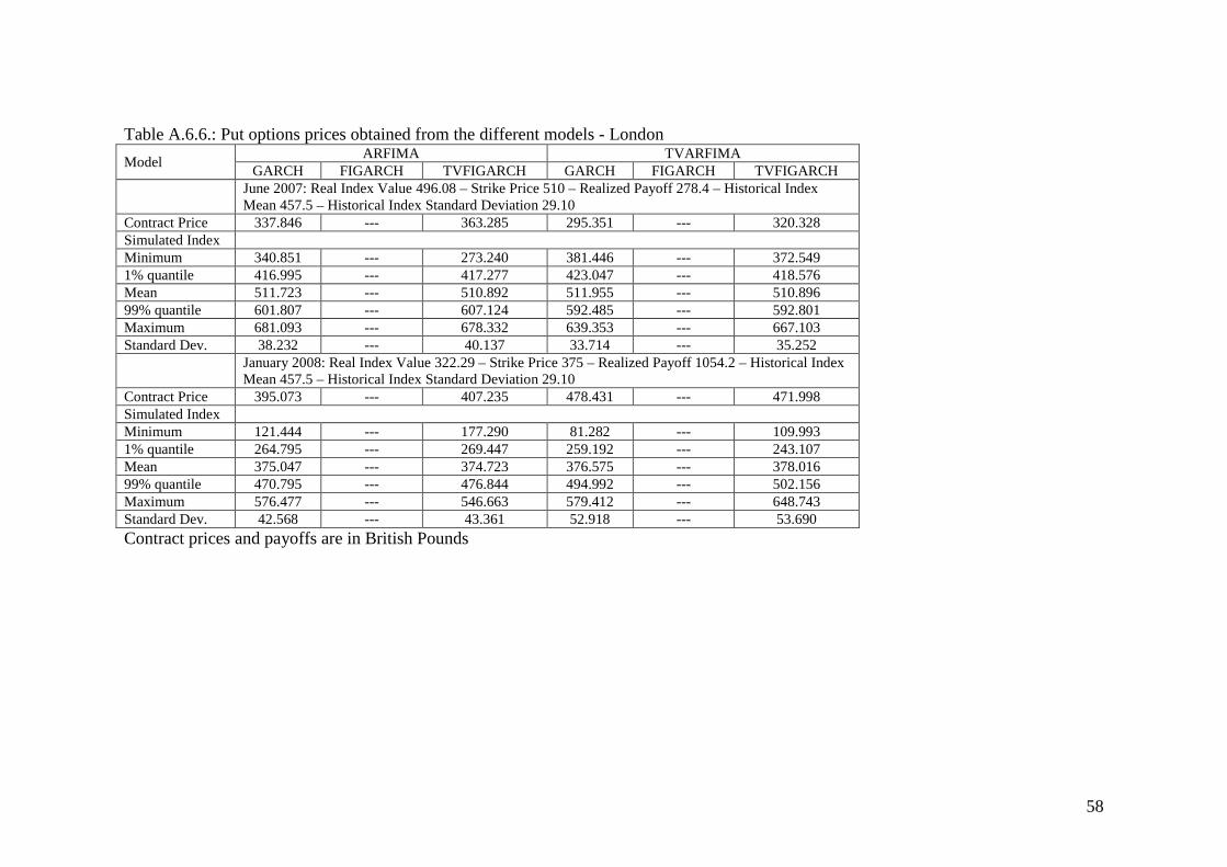
58

Table A.6.6.: Put options prices obtained from the different models - London

Model ARFIMA TVARFIMA

GARCH FIGARCH TVFIGARCH GARCH FIGARCH TVFIGARCH

June 2007: Real Index Value 496.08 – Strike Price 510 – Realized Payoff 278.4 – Historical Index Mean 457.5 – Historical Index Standard Deviation 29.10

Contract Price 337.846 --- 363.285 295.351 --- 320.328 Simulated Index Minimum 340.851 --- 273.240 381.446 --- 372.549 1% quantile 416.995 --- 417.277 423.047 --- 418.576 Mean 511.723 --- 510.892 511.955 --- 510.896 99% quantile 601.807 --- 607.124 592.485 --- 592.801 Maximum 681.093 --- 678.332 639.353 --- 667.103 Standard Dev. 38.232 --- 40.137 33.714 --- 35.252

January 2008: Real Index Value 322.29 – Strike Price 375 – Realized Payoff 1054.2 – Historical Index Mean 457.5 – Historical Index Standard Deviation 29.10

Contract Price 395.073 --- 407.235 478.431 --- 471.998 Simulated Index Minimum 121.444 --- 177.290 81.282 --- 109.993 1% quantile 264.795 --- 269.447 259.192 --- 243.107 Mean 375.047 --- 374.723 376.575 --- 378.016 99% quantile 470.795 --- 476.844 494.992 --- 502.156 Maximum 576.477 --- 546.663 579.412 --- 648.743 Standard Dev. 42.568 --- 43.361 52.918 --- 53.690 Contract prices and payoffs are in British Pounds