universita' degli studi di napoli federico ii department of industrial
TRANSCRIPT

UNIVERSITA' DEGLI STUDI DI NAPOLI FEDERICO II
DEPARTMENT OF INDUSTRIAL ENGINEERING
PH.D. THESIS IN AEROSPACE, MARINE AND QUALITY
ENGINEERING
HYDRODYNAMIC AND STRUCTURAL
CORRELATIONS FOR THE WATER IMPACT OF
HIGH SPEED PLANING CRAFT
Tutors:
Prof. Sergio De Rosa Chairman:
Prof. Francesco Franco Prof. Luigi de Luca
Prof.ssa Ermina Begovic Candidate:
Prof. Carlo Bertorello Ing. Nicola Santoro

2

3
UNIVERSITA' DEGLI STUDI DI NAPOLI FEDERICO II
DEPARTMENT OF INDUSTRIAL ENGINEERING
PH.D. THESIS IN AEROSPACE, MARINE AND QUALITY ENGINEERING
HYDRODYNAMIC AND STRUCTURAL
CORRELATIONS FOR THE WATER IMPACT OF
HIGH SPEED PLANING CRAFT
Tutors:
Prof. Sergio De Rosa Chairman:
Prof. Francesco Franco Prof. Luigi De Luca
Prof.ssa Ermina Begovic Candidate:
Prof. Carlo Bertorello Ing. Nicola Santoro

4

5
Preface
The analysis of the water impact of a rigid body finds a lot of
applications in different engineering field: civil, mechanical,
aeronautical, naval, etc.
For instance, in civil engineering the problem is for the bridge pillars
into a river, in the aerospace field the airplane or helicopters sea landing
is widely studied phenomenon and so on for the other engineering
phenomena.
One of the most important applications can be found in naval field,
where the slamming phenomenon is widely studied for the high stress
caused on the structure.
The analytical formulation of the slamming phenomenon has been
studied by different authors, following both 2D and 3D approaches. Of
course, the second one, with 3D geometry and forward speed with
incident waves, takes into account more effects than 2D theories, but it
complicates the impact analysis to a situation that does not seem
feasible to easy solve by numerical methods at moment.
Thus, this work is focused on the theoretical 2D formulation, useful to
have a prediction before the direct measurements of the pressure
through a wide experimental campaign.
This thesis characterizes the dynamic water impact for the high speed
planing craft and the hydrodynamic and structural correlations, between
different sizes of models, are implemented.
In literature, the analytical and the experimental studies of the water
impact problem have been analysed looking only to a single impact into
water, neglecting the craft forward speed, the trim angle, the air
incursion and other effects; so, the peculiarity of this work is that, the
time history of a run, with various impacts, is studied, in order to have a

6
complete frequency analysis, useful to characterize the dynamic
structural behaviour of the hull bottom panels.

7
Introduction
In the marine field, the water impact of the bow is usually called
slamming. This phenomenon is different for low speed vessels (Figure
1.1) and high speed planing craft (Figure 1.2); in the first case the
slamming is a rare event and the study of it could be treated by a
statistical approach, for the second case the slamming phenomenon is
defined as the re-entry into water after the craft becomes partially
airborne; this is a periodic event and the study of it should be done
following a deterministic approach both in time and frequency domain.
Figure 1.1: Slamming for low speed vessels
Figure 1.2: Slamming for high speed planing craft

8
The slamming pressure assessment is an important topic for shell
plating and stiffener design of bow flare.
In the first part of this work, the pressure distribution on the bottom
plating of a high speed planing craft is evaluated through measurements
of the impact pressures on scale model running in regular waves.
The planing hull model is a monohedral hard chine, built with clear
bottom and deck, in order to allow the visual inspection of the fluid
flow and the exact points of impact. It has been extensively studied in
previous works.
From the time histories of vertical motions (heave and pitch) and bow
acceleration of the model measured in “standard” seakeeping tests,
preliminary assessment of the slamming impact pressure according to
Zhao and Faltinsen (2005) method is performed. The experimental
campaign presented in this first part is focused on the pressure field
assessment in nine points of the hull bottom surface running at four
velocities and two regular waves. Results analysis in time and
frequency domain is given, identifying the pressure distribution along
the bottom panel. Furthermore, comparison of measured, analytical and
normative values has been performed.
In the second part of the thesis, after the hydrodynamic phenomenon
analysis, the elastic behaviour of different bottom panels is predicted.
In order to study a real case, after the scantlings of a real planing craft
bottom panels, with four different materials, an analytical and
numerical modal analysis is performed and a scaling method is
implemented, in order to obtain the scale panels with the same
structural dynamic behaviour.
As final step, a preliminary dynamic analysis of the panels, under the
hydrodynamic load, is performed; this has been done in order to
analyse which characteristic structural natural frequencies are more

9
excited and if this behaviour is well correlated with full scale. It is
useful to see which panels characteristic frequencies are more excited
and the maximum displacement of the panels, because it is possible to
have an indication about which frequencies to avoid due to machinery
equipment (engine, shaft, generators, etc.).

10

11
TABLE OF CONTENTS
1. STATE OF ART............................................................................................ 17
1.1 Dynamic impact ....................................................................................... 17
1.2 Slamming.................................................................................................. 18
1.2.1 Water entry problem ......................................................................... 18
1.3 Similitude ................................................................................................. 21
1.4 Experimental methods and scaling laws for water impact ....................... 22
2. HYDRODYNAMIC AND IMPACT PRESSURE PREDICTION ........... 25
2.1 Water impact on rigid bodies ....................................................................... 25
2.2 Experimental set-up ...................................................................................... 28
2.3 Seakeeping tests and pressure evaluation ..................................................... 30
3. HYDRODYNAMIC AND IMPACT PRESSURE MEASUREMENT .... 35
3.1 Experimental set-up and instruments ........................................................... 35
3.2 Experimental tests results and analysis ........................................................ 37
3.2.1 Pressure values ....................................................................................... 37
3.2.2 Analysis in the frequency domain .......................................................... 46
3.2.3 Results comparison ................................................................................ 50
4. PRELIMINARY INVESTIGATION ON THE DYNAMIC
BEHAVIOUR OF DIFFERENT BOTTOM PANELS ................................. 53
4.1 Scantlings of full scale bottom panels .......................................................... 53
4.2 Modal analysis and scantlings of the panels ................................................ 55
4.3 Preliminary dynamic analysis of the panels under the hydrodynamic
load .................................................................................................................. 59

12
4.3.1 Hydrodynamic load definition .......................................................... 60
4.3.2 Dynamic analysis results ................................................................... 60
5. CONCLUSIONS ........................................................................................... 65
APPENDIX A ................................................................................................... 67
Part I .................................................................................................................. 67
Part II ................................................................................................................ 83
APPENDIX B .................................................................................................... 87
PART I .............................................................................................................. 87
Part II ................................................................................................................ 94
6. ACKNOLEDGMENTS ................................................................................ 97
Bibliography ..................................................................................................... 99

13
Tables of Figures
Figure 1.1: Slamming for low speed vessels .................................................................................................. 7
Figure 1.2: Slamming for high speed planing craft ........................................................................................ 7
Figure 2.1: von Karman wedge .................................................................................................................... 25
Figure 2.2: Wagner wedge ........................................................................................................................... 27
Figure 2.3: Experimental set-up ................................................................................................................... 29
Figure 2.4: Amplitude of vertical motions at bow ........................................................................................ 30
Figure 2.5: Vertical accelerations at bow ..................................................................................................... 31
Figure 2.6: Predictions of pressure (p) distribution during water entry of a rigid wedge with
constant vertical velocity V .......................................................................................................................... 31
Figure 2.7: Zhao and Faltinsen diagram of hydrodynamic pressure distribution .......................................... 32
Figure 2.8: : Comparison between predicted pressure trend for three forward speed ................................... 33
Figure 3.1: Pressure sensor model EPX-N02-1,5B-/Z2 ................................................................................ 35
Figure 3.2: Static calibration system ............................................................................................................ 36
Figure 3.3: Sensor position ........................................................................................................................... 36
Figure 3.4: Main measured values during a run at forward speed of 6.32 m/s ............................................. 38
Figure 3.5: Pressure trend for positions (a) A1 A2 A3, (b) B1 B2 B3 and (c) C1 C2 C3 at model
speed 6.32 m/s .............................................................................................................................................. 40
Figure 3.6: Characteristic values p1/3, p1/10 and pmean of the pressure peaks, at point A1, in function
of forward speed ........................................................................................................................................... 41
Figure 3.7: Characteristic values p1/3, p1/10 and pmean of the pressure peaks, at point A2, in function
of forward speed ........................................................................................................................................... 41
Figure 3.8: Characteristic values p1/3, p1/10 and pmean of the pressure peaks, at point A3, in function
of forward speed ........................................................................................................................................... 41
Figure 3.9: Pressure field at v= 3.4 and 4.6 m/s ........................................................................................... 42
Figure 3.10: Pressure field at v = 5.57 and 6.32 m/s .................................................................................... 43
Figure 3.11: Impact pressure mean values for the longitudinal position A1, A2 and A3 ............................. 44
Figure 3.12: Impact pressure mean values in point A1................................................................................. 45
Figure 3.13: Single peak of pressure for test condition 4 at position A1 ...................................................... 46
Figure 3.14: Transfer from time to frequency domain ................................................................................. 47
Figure 3.15: Pressure FFT for points A1, A2, A3 at model speed 6.32 m/s ................................................. 48
Figure 3.16: FFT of vertical acceleration and encounter wave amplitude at model speed 6.32 m/s ............. 48
Figure 3.17: Cross-correlation analysis between pressure, acceleration and wave at point A2 at
model speed of 6.32 m/s ............................................................................................................................... 49
Figure 3.18: Comparison between measured and analytical hydrodynamic pressure at point A1 ................ 50
Figure 4.1: Full-scale craft Gagliotta 44 ....................................................................................................... 53
Figure 4.2: Structures plan of the full-scale craft ......................................................................................... 54
Figure 4.3: (a) mode 1, (b) mode 2 and (c) mode 3 of composite scale panels............................................. 59

14
Figure 4.4: Glass fiber composite panel dynamic response at model speed of 5.53 m/s .............................. 61
Figure 4.5: Glass-kevlar fiber composite panel dynamic response at model speed of 5.53 m/s ................... 61
Figure 4.6: Carbon fiber composite panel dynamic response at model speed of 5.53 m/s .......................... 62
Figure 4.7: Aluminium panel dynamic response at model speed of 5.53 m/s............................................... 62

15
List of Tables
Table 2.1: Model characteristics ................................................................................................................... 29
Table 2.2: Seakeeping test conditions .......................................................................................................... 30
Table 2.3: Zhao and Faltinsen slamming parameters ................................................................................... 32
Table 3.1: Test conditions for pressure measurements ................................................................................. 37
Table 3.2: Pressure sensors positions ........................................................................................................... 37
Table 3.3: Scheme of the scale-down method .............................................................................................. 50
Table 4.1: Full-scale glass fiber composite and aluminium panels characteristics ....................................... 54
Table 4.2: Full-scale kevlar-glass fiber and carbon fiber composite panels characteristics .......................... 54
Table 4.3: Natural frequencies for full-scale glass fiber composite panel and aluminium panel .................. 56
Table 4.4: Natural frequencies for full-scale kevlar-glass fiber and carbon fiber composite panels ............. 56
Table 4.5: Model scale glass fiber composite and aluminium panels characteristics ................................... 57
Table 4.6: Model scale kevlar-glass fiber and carbon fiber composite panels characteristics ...................... 58
Table 4.7: Natural frequencies for scale glass fiber composite panel and aluminium panel ......................... 58
Table 4.8: Natural frequencies for scale kevlar-glass fiber and carbon fiber composite panels ................... 58

16

17
1. STATE OF ART
1.1 Dynamic impact
Before approaching the central topic of this thesis, in the first part of
this chapter, the state of art of dynamic impact is briefly introduced.
Most of the structural problems are often studied through static or
quasi-static approaches and the effect of inertia are neglected. The
analysis of dynamic impact, especially on composite materials, is
mentioned below.
In a paper by A. S. Yigit and A. P. Christoforou [1], the dynamics of
composite beam subject to transverse impact is investigated. A
linearized contact law based on an elastic-plastic contact is shown to
yield excellent results for impact response. A dynamic ratio is used to
characterize the type of impact response, i.e. whether it is locally
dominated, quasi-static or dynamic. This ratio is defined as the ratio of
the maximum impact force, obtained from the dynamic simulation,
compared to the one obtained from a half-space analysis (i.e. local
contact).. It is found that this depends on a single dimensionless
parameter called "dynamic impact number", which also governs the
initial impact response until the waves are reflected back from the
boundaries. The contact models used in most impact studies are
traditionally based on the Hertzian contact law [2-4].
Qiao and Yang, in their studies [5, 6], analyse the behaviour of fiber
reinforced polymer honeycomb and soft-core composite sandwich
beams. In these studies a higher-order impact model is presented to
simulate the response of sandwich beam subjected to a foreign impact.
The predicted impact responses (e.g. contact force and central
deflection) are compared with the finite elements simulation by LS-
DYNA. The presented impact analysis demonstrates the accuracy and

18
capability of the higher-order impact sandwich beam theory, it can be
used effectively in analysis, design applications and optimization of
efficient sandwich structures for impact protection and mitigation.
1.2 Slamming
Approaching the study of the dynamic impact, the attention has been
focused on the marine field and on the most common dynamic impact
which occurs against the naval structures: the slamming.
Slamming is defined as the re-entry into water of the ship's bow. This
phenomenon is different for high speed planing craft and low speed
vessels. In the first case the impact on the water is periodic; for the
second case, the slamming is a rare event and the study of it could be
treated by a statistical approach.
Assessment of slamming pressures is important in designing plates and
stiffeners in bow flare, bottom, and possibility flat stern areas of ships
and in the cross structure (wetdeck) of multihulls. Design slamming
pressures are usually obtained by using formulae given by the
classification societies. However, these formulae are fully empirical and
therefore not necessarily valid and thus suitable for novel designs.
Therefore, there is a growing need for direct calculation methods.
1.2.1 Water entry problem
According with the pioneering works by von Karman [7] and Wagner
[8], the pressure determination in impact problems is simplified to the
water entry of a two-dimensional section of a hull (wedge analogy) with
different levels of mathematical accuracy. Zhao (et al.) [9, 10],
Faltinsen [11] and Lewis (et al.) [12]. Zhao and Faltinsen present two
different theoretical methods for predicting slamming loads on two-
dimensional sections. One of the methods [9] (developed in 1993) is a

19
fully non-linear numerical simulation, that includes flow separation
from knuckles or fixed separation points of a body with continuously
curved surface. The other method (1997) [10] present a "generalized
Wagner theory" that is a simplification of the exact solution of the
water entry problem, already presented in [9], and it is an approximate
solution; it does not include the flow separation. "Generalized Wagner
theory" means that the exact boundary conditions are satisfied. All
terms in Bernoulli's equation are included (as shown below) except the
hydrostatic pressure term. If the predicted pressure becomes less than
the atmospheric pressure, pa, the pressure is simply set equal to this
latter. This occurs at the spray root and is caused by the square-velocity
term in Bernoulli's equation.
In their works A. Carcaterra and E. Ciappi [13, 14], provide a
theoretical and experimental analysis of the response of an elastic
system carried on board a wedge-shaped body impacting the water
surface.
Other analytical methods are available from the literature to assess
slamming pressure [15].
Some numerical studies of this phenomenon can be also found;
Hermundstad and Moan in [16, 17] present an efficient numerical
method and applied it to a passengers vessel at Froude number around
0.3 in head and oblique seas. They distinguish two main approaches,
namely the "k-factor methods" and the "direct methods". The k-factors
methods are based on the use of slamming coefficients or so-called k-
factors; these k-factors relate the slamming pressure to the square of the
impact velocity, and they can be calculated, or obtained experimentally,
prior to the ship motion analysis. In a direct method, one starts out with
the ship motion calculations, and then applies the slamming calculation
method each time a slamming event takes place.

20
I. Stenius and A. Rosén [18] consider finite element modelling of the
hydrodynamic loads in hull-water impacts. The aim of that work is to
investigate the modelling of hydrodynamic impact loads by use of the
explicit FE-code LS-DYNA. In another study [19], this software is
used; K. Das and R. C. Batra analyse the local water slamming referred
to the impact of a part of a ship hull on stationary water for a short
duration, during which high local pressures occur on the hull. They
simulate slamming impact of rigid and deformable hull bottom panels
by using the Lagrangian and Eulerian formulations included in the
software LS-DYNA. The great advantage of this modelling technique is
that it enables the modelling of instantaneous fluid-structure interaction.
In heavy sea, slamming and wave impact are observed by Mizoguchi
and Tanizawa [20]. These wave loads are of practical importance for
naval architecture to design a safety ship operator to carry cargoes in
safety. In this review section, the principle phenomenon and the
prediction methods of these wave loads are presented. These include
theories of slamming impact both of Wagner type and Bagnold type and
application of numerical simulation methods to the slamming impact.
Further they also analyse the elastic response of ship structures to
slamming impact loads and long-term prediction theories of slamming
impact loads and the elastic response. In 2008 S. Kim and D. Novak
[21] present the developments at ABS to revise the requirements for
slamming impact loads on high speed naval craft. According to the
ABS Guide for Building and Classing High Speed Naval Craft (HSNC
2007), slamming impact load is one of the most critical factors for the
scantling design of hull structures. Extensive numerical simulations are
carried out using the non-linear time domain seakeeping program
LAMP. This paper also presents ABS's on-going efforts for the
development and validation of computational fluid dynamics (CFD)

21
code as an alternative numerical tool to analyse the extremely violent
non linear free-surface flows such as, sloshing, slamming and green
water impact problem.
Mark Battley, [22], describes a dynamic finite elements analysis based
study of slamming impacts on marine composites panel structures; he
shows that the response is highly dependent on the impact velocity,
dead-rise angle, natural frequency of the panel and the frequency
content of the loading
1.3 Similitude
After understanding the analytical theory of a phenomenon, of course,
any new design is extensively evaluated experimentally until it achieves
the necessary reliability, performance and safety. However, the
experimental evaluation of a structures is costly and time consuming.
Consequently, it is extremely useful if a full-scale structure can be
replaced by a similar (scaled-down) model, which is much easier to be
used. Furthermore, a dramatic reduction in cost and time can be
achieved, if available experimental data of a specific structure can be
used to predict the behaviour of a group of similar system.
Similitude theory is thus employed to develop the necessary similarity
conditions (scaling laws). Scaling laws provide relationship between a
full-scale structure and its scale model, and can be used to extrapolate
the experimental data of a small, inexpensive and testable model into
design information for a large prototype. There are two methods to
develop similarity conditions, the direct use of governing equations and
dimensional analysis. The similarity conditions can be established
either directly from the field equations of the system or, if it is a new
phenomenon and the mathematical model of the system is not available,
through dimensional analysis. The first method is more convenient than

22
dimensional analysis, since the resulting similarity conditions are more
specific. In fact, in this case, the field equations of the system with
proper boundary and initial conditions characterize the behaviour of the
system in terms of its variables and parameters. Examples of the direct
use of governing equations is offered by Simitses [23, 24]: only direct
use of the governing equations procedure is considered. If the field
equations of the scale model and its prototype are invariant under the
transformation, then the two system are completely similar. This
transformation defines the scaling laws among all parameters belonging
to the two system.
By using dimensional analysis [25-28], an incomplete form of the
characteristic equation of the system can be formulated. This equation
is in terms of dimensionless products of variables and parameters of the
system. Then, similarity conditions can be established on the basis of
this equation.
1.4 Experimental methods and scaling laws for water impact
The scaling laws and the related similitude can be applied to a lot of
physical phenomena and engineering problems. In literature it is also
possible to find several applications.
In the marine field the most common application of scaling laws is for
performance prediction of ship models using Froude method.
Furthermore, also for the experimental study of the hydrodynamic
impact, caused by slamming, is useful to apply a similitude method. In
the studies by Lee and Wilson [29] and Manganelli [30], pressure
transducers and a special measurement system named "Slam Patch"
have been designed and implemented to measure the hydro-impact
pressure and/or the local structure's response. The measurement systems
are installed on a 1/7-scale model of an Open 60 yacht. Modal,

23
rotational drop and seakeeping-slamming tests are carried out. The
measured hydro-impact pressure is processed statistically. A
methodology to scale up the test results to prototype is mentioned (force
by λ3, pressure by λ, time by λ1/2
, quantity of force impulse by λ7/2,
quantity of pressure impulse by λ3/2). At the same time, the transient
response of a simple structure under half-sine impulse is calculated
using a commercial finite element analysis program to study the effect
of the relationship between impulse duration and natural frequency of
the structure.
Other experimental studies were been done by M. Battley; in [31]
experimental measurements of transient strains, local acceleration and
pressure are undertaken on the IMOCA Open 60' class sailing yacht,
and on a replica hull panel section tested in a laboratory slam testing
facility; the testing facility used in this study is known as the Servo-
hydraulic Slam Testing System (SSTS).
In other papers Battley describes the use of SSTS to test impact of
marine sandwich panels [32, 33] and of composite hull panels [34]
with water. In fact the sandwich panels are widely used within the
marine industry, particularly as primary hull shell structure, but also as
appendages and deck housing. Hydrodynamic loads can be very
significant for these structures, particularly for high-speed craft.
One of the most important experimental studies about planing pressure
is developed by Garme [35, 36], he describes an experimental study
with the major aim to get a detailed picture of the pressure distribution
carrying a planning craft at high speed through calm water and waves.
The instrumentation, load cases and performed runs are discussed as
well as the steps to use the measurement data for evaluation of
numerical models for planing craft in waves.

24
Other relevant studies concerning the analytical/experimental analysis
about slamming impact are in [37, 38], which characterize slamming
loads acting on fast monohull vessels.
In the next sections an experimental campaign on an high speed planing
craft in regular waves is presented, in order to measure and to analyse
the hydrodynamic and impact pressure; furthermore, an analysis of the
elastic behaviour of four different bottom panels is developed.

25
2. HYDRODYNAMIC AND IMPACT PRESSURE
PREDICTION
2.1 Water impact on rigid bodies
To study the water impact phenomenon, the body can be assumed rigid
in the hydrodynamic calculations. Several approximations can be made
in the analysis. The air-flow is usually not important and so neglected
and irrotational flow of incompressible water can be assumed. Because
the local flow acceleration is large relative to gravitational acceleration
when slamming pressure occurs, gravity acceleration is neglected. The
main references are von Karman [7] and Wagner [8] methods. The first
one does not consider the local rise up of the water around the hull and
it proceeds to calculate the impact force through the application of the
momentum theorem. The original momentum of the body is distributed
at the time t between the body and the water. That part of the
momentum is already transferred to the water at the time t depends on x
and can be approximated as follows. With reference to Figure 2.1
Figure 2.1: von Karman wedge
the total momentum is:

26
which must be equal to the original momentum:
v is the downward velocity, vo is the velocity at moment of first contact,
W is the weight of the body per unit length, β is the deadrise angle and
y and x are the vertical and horizontal distance through which the body
travels in the time t. Setting:
it is obtained
where
writing this in the form
it is easy to calculate
finally, the expression of the impact pressure is given as:
and the average pressure as

27
the pressure is evidently maximum in the middle of the float at the
moment of first contact, therefore
Instead, the Wagner's method take into account the rise-up of the water
and semi-infinite wedge-cylinder idealization, as shown in the Figure
2.2
Figure 2.2: Wagner wedge
Through the Bernoulli equation:
where ϕ is the velocity potential with the following boundary
conditions:

28
for a simple triangular wedge, with deadrise angle β, the expanding
velocity of plate is
Wagner's theory gives the impact pressure as:
Zhao et al. [10] presented a generalized Wagner theory that is a
simplification of the more exact solution of the water entry problem by
Zhao and Faltinsen. The generalized Wagner method is more
numerically robust and faster than the original exact solution. It gives
satisfactory results and is therefore preferred in engineering practice.
2.2 Experimental set-up
To assess the hydrodynamic impact pressure by Faltinsen and Zhao
method, experimental seakeeping tests have been done to obtain the
vertical velocity as input for the analytical procedure.
All experiments are performed in the towing tank (135m x 9m x 4.2m)
of DII, University of Naples Federico II with maximum towing carriage
speed of 7 m/s and a multi-flap wave maker by Edinburgh Design. The
hull model is a monohedral hard chine V bottom, from Begovic and
Bertorello work [39], built with clear bottom and deck in order to allow
the visual inspection of the wetted surface before and after the
slamming impact. From a series of seakeeping tests from Begovic et al.
[40] the resonant wave frequency is identified and it has been chosen as
the first test parameter. Three model velocities have been identified to
cover all operating speed range.

29
Model is connected to carriage by the measuring instrument R47, which
allows model to heave and pitch, but restrict it to surge, sway, roll and
yaw. The main characteristics of the model are reported in Table 2.1
Description Symbol Value
Length over all Loa 1.9 m
Length of the monohedral part Lab 1.5 m
Breadth B 0.424 m
Immersion T 0.096 m
Ship Displacement D 32.66 kg
Longitudinal position of GC from stern LCG 0.73 M
Vertical position of GC from keel VCG 0.145 m
Deadrise angle β 16.7 deg
Table 2.1: Model characteristics
The model is ballasted to achieve a weight of 32.66 kg and trimmed to
1.66 degree. Towing force, directed horizontal to the calm water level,
is applied to the model at deck level (0.18 m from baseline) and at
0.535 m from stern. Pitch and heave are measured at R47 position;
heave at CG is recalculated during data elaboration. Two
accelerometers Cross Bow CXL04GP3-R-AL are mounted at model,
one at CG position and another one at 1.6 m from stern. Encounter
wave amplitude is measured by two ultrasonic wave gauges type
Baumer UNDK 301U6103/SI4, one aligned with the R47 and one 4
meters in the front of measuring arm. The model set-up is shown in
Figure 2.3
Figure 2.3: Experimental set-up

30
All seakeeping data are sampled at frequency of 500 Hz. For purpose of
this work three test conditions are considered, reported in Table 2.2
Wave amplitude [m] Wave frequency [Hz] Model speed
[m/s]
Encounter
Frequency
[Hz]
Test #1 0.032 0.65 3.4 1.56
Test #2 0.032 0.65 4.6 1.91
Test #3 0.032 0.65 5.75 2.21
Table 2.2: Seakeeping test conditions
and the following values are measured: forward speed, heave and pitch
motions, vertical accelerations in two points and encounter wave
(amplitude and frequency).
2.3 Seakeeping tests and pressure evaluation
From the seakeeping tests results, i.e. from the measured heave and
pitch at the centre of the gravity, the vertical motion at the bow is
calculated. Time series of calculated vertical motions at 1.6 meters from
stern are shown in Figures 2.4. Measured accelerations at the bow
section, are shown in the Figure 2.5 for the three different model speed
reported in Table 2.2.
Figure 2.4: Amplitude of vertical motions at bow
-0.02
0.00
0.02
0.04
0.06
0.08
0.10
0 1 2 3 4 5 6 7 8
Ver
tival
mo
tio
ns
z(t)
[m
]
time [s]
z(t) test1 z(t) test2 z(t) test3

31
Figure 2.5: Vertical accelerations at bow
The pressure evaluation is based on the studies presented by Zhao and
Faltinsen [9-11].
The following Figure 2.6, shows the predicted pressures for 20°<β<81°
from the Zhao and Faltinsen study [9].
Figure 2.6: Predictions of pressure (p) distribution during water entry of a rigid wedge
with constant vertical velocity V
The pressure distribution becomes pronouncedly peaked and
concentrated close to the spray root when β<≈20°.
0
0.5
1
1.5
2
0 2 4 6 8
Ver
tica
l ac
cele
rati
on a
t b
ow
[g]
time [s]
Bow acc at 3.4 m/s Bow Acc at 4.6 m/s Bow Acc at 5.75 m/s

32
A measure of spatial extent DSS of high slamming pressure is explained
in Figure 2.7. The results by Zhao and Faltinsen [9] show that DSS has
meaning only when β≤≈20°.
Figure 2.7: Zhao and Faltinsen diagram of hydrodynamic pressure distribution
The pressure coefficient and other parameters, defined in Figure 2.7, are
reported in the following Table 2.3
b[°] Cpmax zmax/Vt DSS/c F3/rV3t
4 503.03 0.5695 0.01499 1503.638
7.5 140.587 0.5623 0.05129 399.816
10 77.847 0.5556 0.09088 213.98
15 33.271 0.5361 0.2136 85.522
20 17.774 0.5087 0.4418 42.485
25 10.691 0.4709 23.657
30 6.927 0.4243 14.139
40 3.266 0.2866 5.477
Table 2.3: Zhao and Faltinsen slamming parameters
where, β is the deadrise angle, Cpmax is the pressure coefficient at
maximum pressure, zmax is the z-coordinate of maximum pressure, c =
0.5πVt, F3 is the vertical hydrodynamic force on the wedge and t is the
time.
Thus, the parameters characterizing slamming on a rigid body with
small deadrise angles are the position and the value of the maximum
pressure, the time duration and the spatial extent of high slamming
33
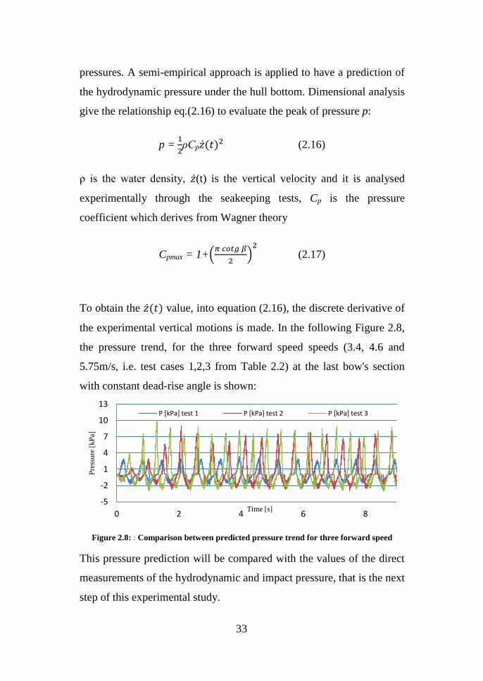
pressures. A semi-empirical approach is applied to have a prediction of
the hydrodynamic pressure under the hull bottom. Dimensional analysis
give the relationship eq.(2.16) to evaluate the peak of pressure p:
p =
ρCp (2.16)
ρ is the water density, (t) is the vertical velocity and it is analysed
experimentally through the seakeeping tests, Cp is the pressure
coefficient which derives from Wagner theory
Cpmax = 1+
(2.17)
To obtain the value, into equation (2.16), the discrete derivative of
the experimental vertical motions is made. In the following Figure 2.8,
the pressure trend, for the three forward speed speeds (3.4, 4.6 and
5.75m/s, i.e. test cases 1,2,3 from Table 2.2) at the last bow's section
with constant dead-rise angle is shown:
Figure 2.8: : Comparison between predicted pressure trend for three forward speed
This pressure prediction will be compared with the values of the direct
measurements of the hydrodynamic and impact pressure, that is the next
step of this experimental study.
-5
-2
1
4
7
10
13
0 2 4 6 8
Pre
ssu
re [
kP
a]
Time [s]
P [kPa] test 1 P [kPa] test 2 P [kPa] test 3

34
The fact that the pressure distribution becomes very peaked illustrates
that measurement of slamming pressure requires high sampling
frequency (as shown below) and small pressure gauges.
In fact, in the most of literature references, experimental errors often
depend on the size of the pressure transducers surface and on the too
low sampling frequency.

35
3. HYDRODYNAMIC AND IMPACT PRESSURE
MEASUREMENT
The major part of the experimental assessment of hydrodynamic impact
pressure is performed for one impact, with the controlled vertical
velocity of the wedge. In this thesis, the impact pressure has been
measured for more realistic scenario, i.e. the boat operating in regular
waves. In fact, analyzing a monohedral planing craft running, it is
possible take into account effects like forward speed, impact with
encounter waves, trim angle, air cushion under the hull bottom and
other frequency components acting on the hull grider.
In this chapter the experimental campaign of the hydrodynamic
pressure measurements on the hull bottom, in different regular waves,
is presented.
3.1 Experimental set-up and instruments
Towing tank, acquisition system and model characteristics are the same
presented for the previous seakeeping tests. Furthermore, for pressure
measurements, the miniature threaded pressure sensors with stainless
flush diaphragm EPX and measuring range from 0 to 1.5 bar have been
adopted. In Figure 3.1, layout and dimensions of this transducer are
shown:
Figure 3.1: Pressure sensor model EPX-N02-1,5B-/Z2

36
Although the calibration certificate for any sensor is available, before
doing the slamming tests, it is need to calibrate the sensors through a
static test, schematically shown in Figure 3.2:
Figure 3.2: Static calibration system
in this way, the right calibration characteristic curve is created.
In the Figure 3.3, positions of the sensors, through the nine threaded
holes on the plexiglass bottom are shown
Figure 3.3: Sensor position
All the data are sampled at frequency of 5000 Hz, this choice is
explained below.

37
In addition to the same conditions of seakeeping tests, other solutions
are performed, reported in Table 3.1
Wave
amplitude
Wave
frequency
Model speed Encounter
Frequency
[m] [Hz] [m/s] [Hz]
Test 1-4 0.032 0.65 3.4-4.6-5.75-6.32 1.56-1.91-2.21-2.37
Test 5-8 0.040 0.65 3.4-4.6-5.75-6.32 1.56-1.91-2.21-2.37
Test 9-12 0.028 0.65 3.4-4.6-5.75-6.32 1.56-1.91-2.21-2.37
Test 13-16 0.020 0.8 3.4-4.6-5.75-6.32 2.21-2.44-3.13-3.36
Test 17-20 0.025 0.8 3.4-4.6-5.75-6.32 2.21-2.44-3.13-3.36
Test 21-24 0.030 0.8 3.4-4.6-5.75-6.32 2.21-2.44-3.13-3.36
Table 3.1: Test conditions for pressure measurements
For the first four test conditions, the pressure in various positions,
represented in Table 3.2, following the layout presented in Figure 3.3, is
measured
Position name. EPX-130KX_14 EPX-130KW_11 EPX-130KV_16
Pos1 A 1 A 2 A 3
Pos2 B 1 B 2 B 3
Pos3 C 1 C 2 C 3
Pos1T C 1 B 1 A 1
Pos2T C 2 B 2 A 2
Pos3T C 3 B 3 A 3
Pos1D C 3 B 2 A 1
Pos2D A 3 B 2 C 1
Table 3.2: Pressure sensors positions
3.2 Experimental tests results and analysis
3.2.1 Pressure values
All the pressure time history, in the investigated positions, are reported
in Appendix A.
The following Figure 3.4 shows the time histories measured during the
test case 4: encounter wave amplitude, heave, pitch, bow’s vertical
accelerations (at 1.6 meters from stern) and the hydrodynamic pressure
under the hull bottom.

38
Figure 3.4: Main measured values during a run at forward speed of 6.32 m/s
An example of the pressure trend in the time domain is reported in
Figure 3.5, where (a), (b) and (c) represent the three sensors
longitudinal positions (see Figure 3.3). In the first group (a) the
longitudinal positions are identified as A1, A2 and A3.
It is possible to observe that the pressure decrease from keel to side, and
also that its trend in the time domain becomes less regular and
influenced by the sprays; this fact could be noted already in the most
external sensors group (c), here reported, and looking at difference
between Figures A1-A12 in the Appendix A..

39
(a)
(b)

40
(c)
Figure 3.5: Pressure trend for positions (a) A1 A2 A3, (b) B1 B2 B3 and (c) C1 C2 C3 at
model speed 6.32 m/s
Obtained pressure data has been analysed in time domain reporting the
mean values of pressure peaks (pmean) and also 1/3rd
and 1/10th
of the
highest (p1/3, p1/10,). In order to illustrate the variation of the values
pmean, p1/3 and p1/10 in function of forward speed, they are represented in
Figures 3.6-3.8. It should be noted that the 1/3rd
and 1/10th
of highest
values here do not have the same meaning as in irregular waves. As the
experiments are performed in regular waves, they should be equal, but
as the measurement of such an impulsive phenomenon presents intrinsic
difficulties they are all reported with an idea to control data elaboration.

41
Figure 3.6: Characteristic values p1/3, p1/10 and pmean of the pressure peaks, at point A1, in
function of forward speed
Figure 3.7: Characteristic values p1/3, p1/10 and pmean of the pressure peaks, at point A2, in
function of forward speed
Figure 3.8: Characteristic values p1/3, p1/10 and pmean of the pressure peaks, at point A3, in
function of forward speed
0
2
4
6
8
10
12
14
3 4 5 6 7
Pre
ssu
re P
eak
[k
Pa]
Speed[m/s]
point A1
0
2
4
6
8
10
12
14
3 5 7
Pre
ssu
re P
eak
[k
Pa]
Speed [m/s]
poinA2
0
2
4
6
8
10
12
14
3 5 7
Pre
ssu
re P
eak
[k
Pa]
Speed [m/s]
point A3

42
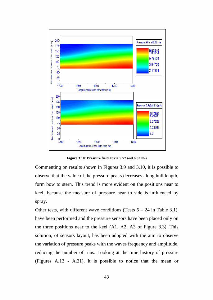
Mean pressure values (pmean) in all points at all model speeds represent
the pressure field on the bottom panel, and is reported in Figures 3.9
and 3.10.
Figure 3.9: Pressure field at v= 3.4 and 4.6 m/s
43
Figure 3.10: Pressure field at v = 5.57 and 6.32 m/s
Commenting on results shown in Figures 3.9 and 3.10, it is possible to
observe that the value of the pressure peaks decreases along hull length,
form bow to stern. This trend is more evident on the positions near to
keel, because the measure of pressure near to side is influenced by
spray.
Other tests, with different wave conditions (Tests 5 – 24 in Table 3.1),
have been performed and the pressure sensors have been placed only on
the three positions near to the keel (A1, A2, A3 of Figure 3.3). This
solution, of sensors layout, has been adopted with the aim to observe
the variation of pressure peaks with the waves frequency and amplitude,
reducing the number of runs. Looking at the time history of pressure
(Figures A.13 - A.31), it is possible to notice that the mean or

44
characteristic value of pressure peaks have a small increase with the
increasing wave amplitude.
In the following Figures 3.11 and 3.12 the dimensionless mean pressure
peak values (pmean/ρgHw), are reported as a function of encounter wave
frequency. In Figure 3.11, the dimensionless impact pressure is reported
for only one encounter wave amplitude, for all three longitudinal
positions nearest to keel, while in Figure 3.12 the impact pressure is
made dimensionless with three different encounter wave height for
position A1 only.
Figure 3.11: Impact pressure mean values for the longitudinal position A1, A2 and A3
0
2
4
6
8
10
12
14
16
18
1.4 1.6 1.8 2.0 2.2 2.4 2.6
Dim
ensi
on
less
pre
ssu
re
Encounter frequency [Hz]
Dimensionless pressure in point A1
Dimensionless pressure in point A2
Dimensionless pressure in point A3

45
Figure 3.12: Impact pressure mean values in point A1
These diagrams shows the phenomenon linearity, changing position
and wave amplitude.
From all figures can be seen that the forward speed is the most
influencing parameter. As regard the effect of wave height variation on
pressure, it can be seen very small variation of pressure for different
wave heights. At the lower speeds there is almost no difference for
different wave height indicating linear dependence on wave amplitude.
At the highest speed, the highest wave amplitude test was not possible
to perform due to water on deck. Measured difference should be seen
more as an experimental uncertainty than as the phenomenon trend.
In this analysis the initial and final transitory part of the signals have
been neglected, in order to observe a more regular phenomenon. To
neglect the lowest frequency phenomena due to initial phase of the
glide, an high-pass filter with a limit frequency of 1.5 Hz has been
applied. Looking at the amplitude of the experimental peaks of
pressure, it is possible to see that it has a very sharp shape (Figure
3.13); in particular, the time step of increasing pressure, during the
0
2
4
6
8
10
12
14
16
18
1.5 1.7 1.9 2.1 2.3 2.5
Dim
ensi
on
less
pre
ssu
re P
/ρgH
w
Encounter frequency [Hz]
P/rgHw56
P/rgHw64
P/rgHw80
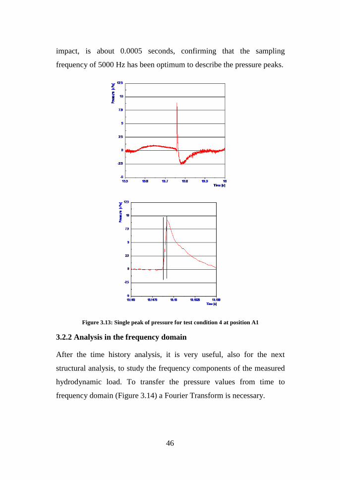
46
impact, is about 0.0005 seconds, confirming that the sampling
frequency of 5000 Hz has been optimum to describe the pressure peaks.
Figure 3.13: Single peak of pressure for test condition 4 at position A1
3.2.2 Analysis in the frequency domain
After the time history analysis, it is very useful, also for the next
structural analysis, to study the frequency components of the measured
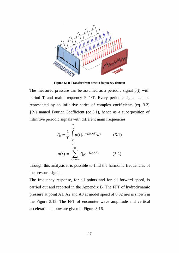
hydrodynamic load. To transfer the pressure values from time to
frequency domain (Figure 3.14) a Fourier Transform is necessary.
47
Figure 3.14: Transfer from time to frequency domain
The measured pressure can be assumed as a periodic signal p(t) with
period T and main frequency F=1/T. Every periodic signal can be
represented by an infinitive series of complex coefficients (eq. 3.2)
{Pn} named Fourier Coefficient (eq.3.1), hence as a superposition of
infinitive periodic signals with different main frequencies.
through this analysis it is possible to find the harmonic frequencies of
the pressure signal.
The frequency response, for all points and for all forward speed, is
carried out and reported in the Appendix B. The FFT of hydrodynamic
pressure at point A1, A2 and A3 at model speed of 6.32 m/s is shown in
the Figure 3.15. The FFT of encounter wave amplitude and vertical
acceleration at bow are given in Figure 3.16.

48
Figure 3.15: Pressure FFT for points A1, A2, A3 at model speed 6.32 m/s
Figure 3.16: FFT of vertical acceleration and encounter wave amplitude at model speed
6.32 m/s
The frequency range of the analysis is up to 35 Hz because over this
frequency the amplitude of the signals is about two order of magnitude
lower than the amplitude at the main frequency. The FFT diagrams of
pressure show that the phenomenon of water impact is characterized by

49
multiple frequencies. Note the first frequency, all the other frequencies
are found to be multiple of the first (f1). For instance, in the case of v =
6.32 m/s the first frequency is equal to 2.45 Hz, the second and the third
ones are equal to f2 = 4.9 Hz and f3 = 7.4 Hz. It was seen in Begovic et
al. [40] that for vertical accelerations higher order harmonics are only
due to the composition of heave and pitch motions; and it is the same
reason for pressure higher order harmonics. To have more information
about the correlation between pressure, vertical acceleration and wave
amplitude, a cross-correlation analysis is done and given in Figure 3.17.
Figure 3.17: Cross-correlation analysis between pressure, acceleration and wave at point
A2 at model speed of 6.32 m/s
At the first characteristic frequency (the main of the measured wave
amplitude) all three signals are well correlated. In order to follow the
previous analysis, for the other characteristic frequencies, only
acceleration and pressure signals are well correlated, because both
values depend from the vertical motions of the model.

50
3.2.3 Results comparison
A comparison between the measured hydrodynamic pressure and those
predicted values by Faltinsen and Zhao at model speed 5.75 m/s and
test case 3 (from Table 2) for point A1 is given in the Figure 3.18. It can
be observed that the maximum peaks are very well predicted, the
difference is about 8%
Figure 3.18: Comparison between measured and analytical hydrodynamic pressure at
point A1
Further comparison with normative values of the hydrodynamic loads
for planing craft (UNI EN ISO 12215) is done. In the following Table
3.3 the way to scale-down the operative conditions is shown using the
methodology adopted by Lee et al [29] and Manganelli [30].
Full Scale model Scale Factor λ Scale model
Shipcharacteristics 6.62 Model characteristics
LS [m] 12.58 LM [m] 1.9
DS[kg] 9460 DM [kg] 32.66
VS [kn] 31.6 VM [m/s] 6.32
β [deg] 16.7 β [deg] 16.7
Fn 1.464 Fn 1.464
Sea conditions Regular wavescharacteristics
H1/3 [m] 0.42 HW [m] 0.064
Design Cat. D fW [Hz] 0.65
Normative Loads Scale Normative Loads
PBMP max S [kPa] 58.7 PBMP max M [kPa] 8.9
PBMP S [kPa] 26.6 PBMP M [kPa] 4.0
Table 3.3: Scheme of the scale-down method

51
L is the length, D is the displacement, V is the forward speed, β the
deadrise angle, Fn the Froude number, H and f are the wave height and
frequency, the PBMP are the normative values of hydrodynamic pressure.
The subscripts S and M indicate the Ship (full scale) and Model (scale).
From the PBMP max values in Table 3.3 it is possible to observe it is quite
similar to the measured one shown in Figure 3.5 for the same
conditions, with about 16% of difference.

52

53
4. PRELIMINARY INVESTIGATION ON THE
DYNAMIC BEHAVIOUR OF DIFFERENT BOTTOM
PANELS
After the understanding of the hydrodynamic phenomenon, and a
review of the different possible methods of load assessment, the
dynamic behaviour of the bottom panels, during the periodic water
impact is investigated. Four different materials representative of the
most used materials in the marine field, are chosen. They are glass-fiber
composite, kevlar-glass fiber composite, carbon-fiber composite and
light alloy 5083 .
4.1 Scantlings of full scale bottom panels
The first step of the analysis is the scantling of a real planing craft
bottom panel. The considered ship is a commercial motor boat, the
Gagliotta 44, shown in Figure 4.1 and 4.2.
Figure 4.1: Full-scale craft Gagliotta 44

54
Figure 4.2: Structures plan of the full-scale craft
After the scantlings procedure, the chosen panel dimensions and
characteristics are carried out and reported in Table 4.1 and 4.2 for each
material
Glass fiber composite panel Aluminium panel
LP 1170 1170 mm
BP 540 540 mm
t 11.1 8.3 mm
y 0.4 - -
E 10200 70000 N/mm2
t/w 1.64 - mm/kg
r 0.0160 0.0220 g/mm2
Weight 10.135 13.897 kg
Table 4.1: Full-scale glass fiber composite and aluminium panels characteristics
Aramide fiber composite panel Carbon fiber composite panel
LP 1170 1170 mm
BP 540 540 mm
t 8.5 6 mm
y 0.5 0.55 -
E 26000 50000 N/mm2
t/w 1.52 1.17 mm/kg
r 0.0120 0.0098 g/mm2
Weight 7.556 6.203 kg
Table 4.2: Full-scale kevlar-glass fiber and carbon fiber composite panels characteristics

55
LP and BP are the panels length and breadth, t is the panels thickness, ψ
is the weight percentage of fiber in the composite, E is the Young
modulus, t/w is the ratio between the thickness and the mass for square
meter of the fiber, and ρ is the panel density.
The hydrodynamic pressure, used for the scantling of this craft, is
calculated using the ISO normative formula. This value is quite similar
to the scaled-up value of the experimental maximum peak on the tested
model.
4.2 Modal analysis and scantlings of the panels
In order to get further information for a better structural design of such
craft, the first three mode shapes frequencies of these panels have been
identified analytically and numerically.
To get an analytical guide-line, the first three natural frequencies are
calculated using formulas for a rectangular plate taken from [41].
According to Blevins, it is possible to obtain the natural frequencies for
different combinations of boundary conditions on the four edges of the
plate, through a dimensionless frequency parameter that is a function of
the boundary conditions, of the aspect ratio and, in some cases, of the
Poisson's ratio of the plate.
After the analytical prediction of the natural frequencies, a numerical
determination has been performed by software Nastran. The results
obtained by the two methods are quite similar, with difference lower
than 5%. The first three natural frequencies (f1, f2 and f3) relative to
full-scale panels are reported on the following Table 4.3 and 4.4

56
Glass fiber composite panel Aluminium panel
E 10200 70000 N/mm2
r 0.0160 0.0220 g/mm2
f1 127.6 178.4 Hz
f2 158.1 221.1 Hz
f3 211.9 296.2 Hz
Table 4.3: Natural frequencies for full-scale glass fiber composite panel and aluminium
panel
Aramide fiber composite panel Carbon fiber composite panel
E 26000 50000 N/mm2
r 0.0120 0.0098 g/mm2
f1 129.0 134.8 Hz
f2 159.9 167.1 Hz
f3 214.3 223.9 Hz
Table 4.4: Natural frequencies for full-scale kevlar-glass fiber and carbon fiber composite
panels
The main dimensions, length and breadth, of the scaled-down panels are
obtained with scale ratio 2, chosen for a practical construction and
fitting on the panels to the model bottom. Instead, the scale panels
thickness is chosen to have a similar dynamic behaviour with the full-
scale panels.
The first step is to identify the dimensionless frequencies representative
of both structural and hydrodynamic phenomena, two kind of relative
frequencies are introduced, eq. (4.1) and eq. (4.2)
f1 is the first natural frequency of the panel, Hw is the wave height, t is
the panel thickness and V is the forward speed.

57
Furthermore, another dimensionless frequency, representative of the
hydrodynamic phenomenon is adopted (4.3):
fe is the wave encounter frequency.
According to the generally used Froude theory Fn is the same for the
scale model and full-scale craft. The thickness of the scale panels is
chosen to achieve the most similar values of the dimensionless
frequencies ,
and between the scale model and the full-size
craft.
After an iterative procedure, the final dimensions of the scale bottom
panels have been carefully chosen, and reported in the following Table
4.5 and 4.6
Glass fiber composite panel Aluminium
panel
LP 585 585 mm
BP 270 270 mm
t 5 3.5 mm
y 0.4 - -
E 10200 70000 N/mm2
t/w 1.64 - mm/kg
r 0.0076 0.00928 g/mm2
Weight 1200 1465 g
Table 4.5: Model scale glass fiber composite and aluminium panels characteristics

58
Aramide fiber composite panel Carbon fiber composite panel
LP 585 585 mm
BP 270 270 mm
t 4 2.5 mm
y 0.5 0.55 -
E 26000 50000 N/mm2
t/w 1.52 1.17 mm/kg
r 0.0048 0.0044 g/mm2
Weight 758 689 g
Table 4.6: Model scale kevlar-glass fiber and carbon fiber composite panels
characteristics
The same modal analysis procedure is used to study the obtained scale
panels.
In the following Table 4.7 and 4.8 the first three natural frequencies,
relative to scale panels, are reported.
Glass fiber composite panel Aluminium
panel
E 10200 70000 N/mm2
r 0.076 0.00928 g/mm2
f1 229.9 300.9 Hz
f2 284.9 372.9 Hz
f3 381.7 499.6 Hz
Table 4.7: Natural frequencies for scale glass fiber composite panel and aluminium panel
Aramide fiber composite panel Carbon fiber composite panel
E 26000 50000 N/mm2
r 0.0048 0.0044 g/mm2
f1 242.9 224.7 Hz
f2 301.0 278.4 Hz
f3 403.3 373.1 Hz
Table 4.8: Natural frequencies for scale kevlar-glass fiber and carbon fiber composite
panels
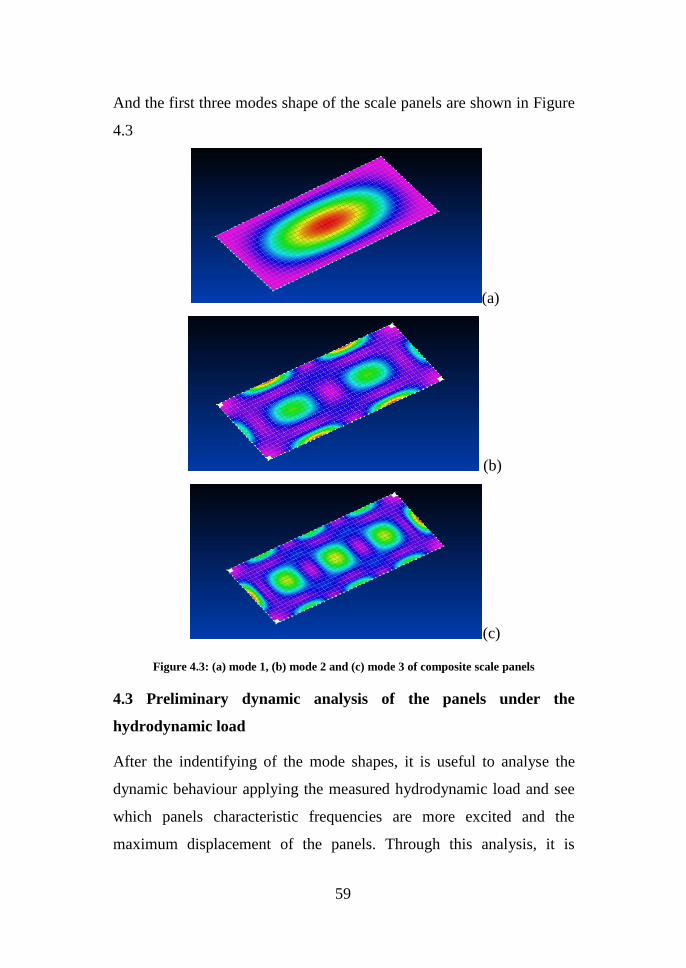
59
And the first three modes shape of the scale panels are shown in Figure
4.3
(a)
(b)
(c)
Figure 4.3: (a) mode 1, (b) mode 2 and (c) mode 3 of composite scale panels
4.3 Preliminary dynamic analysis of the panels under the
hydrodynamic load
After the indentifying of the mode shapes, it is useful to analyse the
dynamic behaviour applying the measured hydrodynamic load and see
which panels characteristic frequencies are more excited and the
maximum displacement of the panels. Through this analysis, it is

60
possible to have an indication about which frequencies to avoid due to
machinery (engine, shaft, generators, ecc) or to hydrodynamic loads.
4.3.1 Hydrodynamic load definition
Changing the model dimensions, it is necessary to adapt also the values
of forward speed and hydrodynamic pressure, following the Froude
method as applied in [30]. Furthermore, the pressure values are
available only for the nine measurement points (see Figure 3.3). To get
the pressure distribution along all panel surface, an interpolation
equation for each forward speed is proposed:
In the previous equations p is the pressure value as function of x and y
coordinates of the bottom panel and provides the pressure distribution
in the space domain for one time instant.
To implement a dynamic analysis, the software FEMAP is adopted for
the NASTRAN model pre-processing.
Imposed the geometry and mesh characteristics of the flat plate, all the
four edges are set as fixed constraints; the measured hydrodynamic
load is introduced as distributed with the time variation experimentally
measured. The analysis is implemented for the four material
characteristics, before presented, and for three different load conditions.
4.3.2 Dynamic analysis results
Some examples of the dynamic analysis results for the chosen materials
panels at forward speed of 5.53 m/s is reported in Figures 4.4 - 4.7.

61
Figure 4.4: Glass fiber composite panel dynamic response at model speed of 5.53 m/s
Figure 4.5: Glass-kevlar fiber composite panel dynamic response at model speed of 5.53
m/s
0
50
100
150
200
250
300
350
400
450
150 200 250 300 350 400
Acc
eler
atio
n [
m/s
2]
Frequency [Hz]
0
50
100
150
200
250
300
350
400
450
150 200 250 300 350 400 450
Acc
ele
rari
on
[m
/s2 ]
Frequency [Hz]

62
Figure 4.6: Carbon fiber composite panel dynamic response at model speed of 5.53 m/s
Figure 4.7: Aluminium panel dynamic response at model speed of 5.53 m/s
It is possible to observe, for the considered forward speed and for the
glass fiber composite panel, that the most excited mode shape is the
third one at frequency of 358 Hz, with an acceleration of 424 m/s2
which corresponds to the maximum deflection of 3.3 mm.
This results have been carried out for all forward speed.
The next step will be the implementation of an Experimental Modal
Analysis (EMA) procedure to the considered panels aimed at
0
100
200
300
400
500
600
700
800
100 150 200 250 300 350 400
Acc
ele
rati
on
[m
/s2 ]
Frequency [Hz]
0
100
200
300
400
500
600
700
800
200 250 300 350 400 450 500
Acc
ele
rati
on
[m
/s2]
Frequency [Hz]

63
determining FRF (Frequency Response Function) of each panel and a
numerical-experimental correlation.

64

65
5. CONCLUSIONS
After the analytical study of the water entry of a rigid wedge through
the Zhao and Faltinsen approach, following the Wagner theory, a
prediction of the hydrodynamic pressure has been carried out starting
from the common seakeeping tests results.
In the next step, the impact of water on a monohedral planing craft has
been studied experimentally in regular waves at four model velocities
measuring hydrodynamic pressure on the bottom by nine sensors and
comparing them with the predicted ones.
Analysis of measured data identified multiple frequencies responses of
pressure and accelerations due to the motions combination. In the
considered range of wave heights, the pressure behaviour is found
almost linear. At all tested velocities the maximum pressure field has
been close to the keel, and decreases moving offset from the centreline.
The pressure reaches its maximum value at the forward position and
decreases going aft.
After the results analysis, a correlation between model and real craft has
been done with the aim to have also a comparison with the normative
values of the pressure.
As a further contribution to the structural design procedure a description
of the dynamic behaviour of the bottom panels made by four different
materials has been analysed in ship and model scale by NASTRAN
software reporting first three natural frequencies and the dynamic
response under the hydrodynamic load action. Particular attention has
been paid to define the dimensionless frequencies which will describe
scaling effect properly.
The next steps of this study will be the Experimental Modal Analysis
(EMA) of the panels in model scale, after assembling to the hull bottom

66
in dry condition, and the Operational Modal Analysis (OMA) during
the towing tests in the towing tank. The scheduled experimental
campaign is aimed at verifying the representation of the phenomenon in
model scale and at observing the eventual hydro-elastic coupling
effects, through the comparison of the Frequency Response Functions.
67
APPENDIX A
PART I
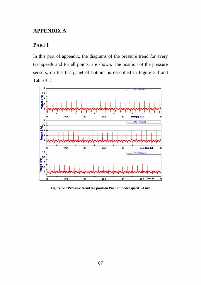
In this part of appendix, the diagrams of the pressure trend for every
test speeds and for all points, are shown. The position of the pressure
sensors, on the flat panel of bottom, is described in Figure 3.3 and
Table 3.2.
Figure A1: Pressure trend for position Pos1 at model speed 3.4 m/s

68
Figure A.2: Pressure trend for position Pos1 at model speed 4.6 m/s
Figure A.3: Pressure trend for position Pos1 at model speed 5.75 m/s
69
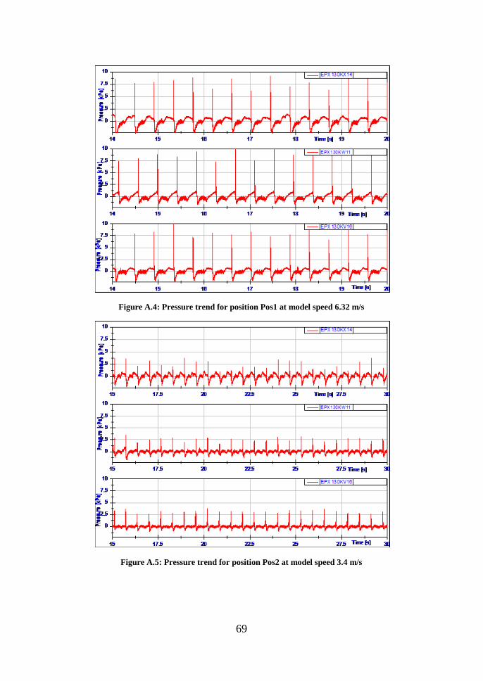
Figure A.4: Pressure trend for position Pos1 at model speed 6.32 m/s
Figure A.5: Pressure trend for position Pos2 at model speed 3.4 m/s

70
Figure A.6: Pressure trend for position Pos2 at model speed 4.6 m/s
Figure A.7: Pressure trend for position Pos2 at model speed 5.75 m/s

71
Figure A.8: Pressure trend for position Pos2 at model speed 6.32 m/s
Figure A.9: Pressure trend for position Pos3 at model speed 3.4 m/s

72
Figure A.10: Pressure trend for position Pos3 at model speed 4.6 m/s
Figure A.11: Pressure trend for position Pos3 at model speed 5.75 m/s

73
Figure A.12: Pressure trend for position Pos3 at model speed 6.32 m/s
Figure A.13: Pressure trend for position Pos1 at Test 5

74
Figure A.14: Pressure trend for position Pos1 at Test 6
Figure A.15: Pressure trend for position Pos1 at Test 7

75
Figure A.16: Pressure trend for position Pos1 at Test 9
Figure A.17: Pressure trend for position Pos1 at Test 10

76
Figure A.18: Pressure trend for position Pos1 at Test 11
Figure A.19: Pressure trend for position Pos1 at Test 12

77
Figure A.20: Pressure trend for position Pos1 at Test 13
Figure A.21: Pressure trend for position Pos1 at Test 14

78
Figure A.22: Pressure trend for position Pos1 at Test 15
Figure A.23: Pressure trend for position Pos1 at Test 16

79
Figure A.24: Pressure trend for position Pos1 at Test 17
Figure A.25: Pressure trend for position Pos1 at Test 18

80
Figure A.26: Pressure trend for position Pos1 at Test 19
Figure A.27: Pressure trend for position Pos1 at Test 20

81
Figure A.28: Pressure trend for position Pos1 at Test 21
Figure A.29: Pressure trend for position Pos1 at Test 22

82
Figure A.30: Pressure trend for position Pos1 at Test 23
Figure A.31: Pressure trend for position Pos1 at Test 24

83
PART II
In the second part the diagrams of measured wave amplitude and
vertical accelerations at the line 2 of points as well as represented in the
Figure 2.5 are reported.
Figure A.32: Vertical accelerations and wave amplitude at model speed 3.4 m/s

84
Figure A.33: Vertical accelerations and wave amplitude at model speed 4.6 m/s
Figure A.34: Vertical accelerations and wave amplitude at model speed 5.75 m/s

85
Figure A.35: Vertical accelerations and wave amplitude at model speed 6.32 m/s

86

87
APPENDIX B
PART I
In this part of appendix, the Fourier Transform of the pressure for every
test speeds and for all points, is shown. The position of the
measurement points, on the flat panel of bottom, is described in Figure
3.3 and Table 3.2.
Figure B.1: Pressure FFT for position Pos1 at model speed 3.4 m/s

88
Figure B.2: Pressure FFT for position Pos1 at model speed 4.6 m/s
Figure B.3: Pressure FFT for position Pos1 at model speed 5.75 m/s

89
Figure B.4: Pressure FFT for position Pos1 at model speed 6.32 m/s
Figure B.5: Pressure FFT for position Pos2 at model speed 3.4 m/s

90
Figure B.6: Pressure FFT for position Pos2 at model speed 4.6 m/s
Figure B.7: Pressure FFT for position Pos2 at model speed 5.75 m/s

91
Figure B.8: Pressure FFT for position Pos2 at model speed 6.32 m/s
Figure B.9: Pressure FFT for position Pos3 at model speed 3.4 m/s

92
Figure B.10: Pressure FFT for position Pos3 at model speed 4.6 m/s
Figure B.11: Pressure FFT for position Pos3 at model speed 5.75 m/s

93
Figure B.12: Pressure FFT for position Pos3 at model speed 6.32 m/s

94
PART II
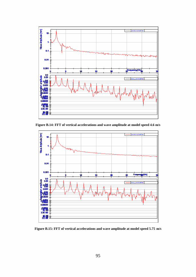
In the second part the FFT diagrams of measured wave amplitude and
vertical accelerations at the line 1 of points as well as represented in the
Figure 3.3, are presented
Figure B.13: FFT of vertical accelerations and wave amplitude at model speed 3.4 m/s
95
Figure B.14: FFT of vertical accelerations and wave amplitude at model speed 4.6 m/s
Figure B.15: FFT of vertical accelerations and wave amplitude at model speed 5.75 m/s

96
Figure B.16: FFT of vertical accelerations and wave amplitude at model speed 6.32 m/s

97
6. ACKNOLEDGMENTS
Author would like to acknowledge all the staff of the "towing tank" of
Department of Industrial Engineering of the University of Naples
Federico II and Dr. A Bove for his important support to entire
experimental campaign and instruments set up. Furthermore a huge
acknowledgment to all Ph.D. tutors for their dedication to this project.

98

99
BIBLIOGRAPHY
[1] A. S. Yigit and A. P. Christoforou, "Impact dynamics of
composite beams," Composite Structures, vol. 32, pp. 187-195,
1995.
[2] C. T. Sun, "An analytical method for evaluation of impact
damage energy of laminated composites," presented at the
Composite Materials: Testing and Design (fourth edition),
Philadelphia, PA, 1977.
[3] A. L. Dobyns, "Analysis of simply-supported orthotropic plates
subject to static and dynamic loads," AIAA Journal, vol. 19, pp.
642-650, 1981.
[4] S. H. Yang and C. T. Sun, "Indentation law for composite
laminates," presented at the Composite Materials: Testing and
Design (sixth edition), Philadelphia, PA, 1982.
[5] M. Yang and P. Qiao, "Higher-order impact modeling of
sandwich structures with flexible core," International Journal of
Solids and Structures, vol. 42, pp. 5460-5490, 2005.
[6] P. Qiao and M. Yang, "Impact analysis of fiber reinforced
polymer honeycomb composite sandwich beams," Composite
Part B, vol. 38, pp. 739-750, 10 Mar 2006 2007.
[7] T. V. Karman, "The impact of seaplane floats during landing,"
NACA, vol. Tech. note no. 321, 1929.
[8] J. D. Wagner, "Landing of seaplanes," National Advisory
Committee for Aeronautics, vol. TN 622, 1932.
[9] R. Zhao and O. Faltinsen, "Water entry of two-dimensional
bodies," Journal of Fluid Mechanics, vol. 246, pp. 593-612,
1993.
[10] R. Zhao, et al., "Water Entry of Arbitrary Two-Dimensional
Sections with and without Flow Separation," presented at the
Twenty-First Symposium on Naval Hydrodynamics, 1997.
[11] O. M. Faltinsen, Ed., Hydrodynamics of High-Speed Marine
Vehicles. 2005, p.^pp. Pages.
[12] S. G. Lewis, et al., "Impact of free-falling wedge with water:
synchronized visualization, pressure and acceleration
measurements," Fluid Dynamics Research, vol. 42, pp. 1-30, 16
March 2010 2010.
[13] E. Ciappi, "Impact of rigid and elastic structures on the water
surface," Ph. D. in Meccanica teorica e applicata, Dipartimento di
Meccanica e Aeronautica, La Sapienza, Roma.

100
[14] A. Carcaterra and E. Ciappi, "Hydrodynamic shock of elastic
structures impacting on the water: theory and experiments,"
Journal of Sound and Vibration, vol. 271, pp. 411-439, 2004.
[15] X. Mei, et al., "On the water impact of general two-dimensional
sections," Applied Ocean Research, vol. 21, pp. 1-15, 1999.
[16] O. A. Hermundstad and T. Moan, "Efficient calculation of
slamming pressures on ships in irregular seas," Journal of Marine
Science and Technology, vol. 12, pp. 160-182, 2007.
[17] O. A. Hermundstad and T. Moan, "Pratical calculation of
slamming pressures in irregular oblique seas," presented at the
International Conference on Fast Sea Transportation, Athens,
Greece, 2009.
[18] I. Stenius and A. Rosén, "FE - Modelling of hydrodynamic hull-
water impact loads," presented at the 6th European LS-DYNA
Users' Conference.
[19] K. Das and R. C. Batra, "Local water slamming impact on
sandwich composite hulls," Journal of Fluids and Structures, vol.
27, pp. 523-551, 2011.
[20] Sumitoshi Mizoguchi and K. Tanizawa, "Impact Wave Loads due
to Slamming { A Review," Ship Technology Research, vol. 43,
1996.
[21] S. P. Kim, et al., "Slamming impact design loads on large high
speed naval craft," presented at the International Conference on
innovative approaches to further increase speed of fast marine
vehicles, moving above, under and in water surface, Saint-
Petersburg, Russia, 2008.
[22] M. Battley and D. Svensson, "Dynamic response of marine
composites to slamming loads," ed. Engineering Dynamics
Department, Industrial Research Limited - Auckland, New
Zealand, 2001.
[23] G. J. Simitses, et al., "Structural Similitude and Scaling Laws for
Plates and Shells: A Review
Advances in the Mechanics of Plates and Shells." vol. 88, D. Durban, et
al., Eds., ed: Springer Netherlands, 2002, pp. 295-310.
[24] G. J. Simitses and J. Rezaeepazhand, "Title," unpublished|.
[25] P. W. Bridgman, Dimensional Analysis, II ed. New Haven - Yale
University, 1931.
[26] A. A. Sonin, "Title," unpublished|.
[27] E. O. Macagno, "Historico-critical review of dimensional
analysis," Journal of the Franklin Institute, vol. 292, pp. 391-402,
1971.

101
[28] E. Buckingham, "On Physically similar systems illustrations of
the use of dimensional equations," Physics Reviews, vol. IV, pp.
345-376, 1914.
[29] June Lee and P. A. Wilson, "Experimental study of the hydro-
impact of slamming in a modern racing sailboat," Journal of
Sailboat Technology, 26-08-2009 2010.
[30] P. Manganelli, et al., "Investigation of slamming loads using slam
patches on a scale model of an open 60' class yacht," presented at
the The international HISWA Symposium on yacht design and
yacht construction, 2002.
[31] M. Battley, et al., "Structural Responses of High Performance
Sailing Yachts to Slamming Loads," presented at the 11th
International Conference on Fast Sea Transportation, Honolulu,
Hawaii, USA, 2011.
[32] M. Battley and T. Allen, "Dynamic performance of marine
sandwich panel structures," presented at the 18th International
Conference on composite materials, 2011.
[33] M. Battley and T. Allen, "Servo-hydraulic System for Controlled
Velocity Water Impact of Marine Sandwich Penels,"
Experimental Mechanics, vol. 52, pp. 95-106, 29 August 2011
2012.
[34] M. Battley, et al., "Effetcs of panels stiffness on slamming
responses of composite hull panels," ed. Cantre for Advanced
Composite Materials, University of Auckland, 2009.
[35] K. Garme, "Modeling of planing craft in waves," ed, 2004.
[36] K. Garme, et al., "In Detail Investigation of planing pressure,"
presented at the HYDRALAB III, Hannover, 2010.
[37] L. Sebastiani, et al., "A Theoretical / Experimental investigation
of the slamming pressures on fast monohull vessels," presented at
the FAST 2001, Southampton, UK, 2001.
[38] J.-M. Rousset, et al., "Slamming experiments on a ship model,"
ed.
[39] E. Begovic and C. Bertorello, "Resistance assessment of warped
hullform," Ocean Engineering vol. 56, pp. 28 - 42 2012.
[40] E. Begovic, et al., "Experimental Seakeeping Assessment of
Warped Planing Hull," Ocean Engineering, vol. 83, pp. 1-15, 1
June 2014 2014.
[41] R. D. Blevins, Ed., Formula for natural frequency and mode
shape. Malabar, Florida: Robert E. Krieger Publishing Company,
1979, p.^pp. Pages.