understanding the improved performance of disadvantaged...

1

WP21 Understanding the improved performance of disadvantaged pupils in London

Understanding the improved performance of disadvantaged pupils in London

Jo Blanden, Ellen Greaves, Paul Gregg, Lindsey Macmillan and Luke Sibieta

Working Paper 21 September 2015

2


Acknowledgements

This project is part of the Social Policy in a Cold Climate programme funded by the Joseph Rowntree Foundation, the Nuffield Foundation, and Trust for London. Co-funding from the ESRC-funded Centre for the Microeconomic Analysis of Public Policy at the Institute for Fiscal Studies (grant reference ES/H021221/1) is gratefully acknowledged. The authors would also like to thank the Social Mobility and Child Poverty Commission for providing funding for an earlier report, which the paper draws upon. The authors would also like to thank Damon Clark for assistance using the Youth Cohort Study. The Millennium Cohort Study was made available through the Secture Data Service at the UK Data Service and was funded by the ERSC and Government Departments. This paper has benefited from comments from Anna Vignoles, Steve Gibbons, Sandra McNally and Ruth Lupton. We have also received helpful feedback at seminars at CASE, the Department of Quantitative Social Science at UCL, Institute of Education andNuffield College, Oxford.The views expressed are those of the authors and not necessarily those of the funders. More information about the SPCC research programme and can be found at: http://sticerd.lse.ac.uk/case/_new/research/Social_Policy_in_a_Cold_Climate.asp

Authors

Jo Blanden, Senior Lecturer and Deputy Head of School of Economics, University of Surrey and Centre for Economic Performance, London School of Economics.

Ellen Greaves, Senior Research Economist, Education, Employment and Evaluation sector, Institute for Fiscal Studies.

Paul Gregg, Professor of Economic and Social Policy, and Director of the Centre for Analysis and Social Policy at the University of Bath.

Lindsey Macmillan, Senior Lecturer in Economics, Department of Quantitative Social Science, UCL Institute of Education.

Luke Sibieta, Programme Director, Education and Skills sector, Institute for Fiscal Studies

3


Contents

Summary .................................................................................................................................................... 5

1. Introduction .......................................................................................................................................... 6

2. Background: London and London’s Schools ....................................................................................... 9

3. Data ................................................................................................................................................... 11

National Pupil Database Data ............................................................................................................... 12

Youth Cohort Study .............................................................................................................................. 13

Millennium Cohort Study ....................................................................................................................... 15

4. Basic Empirical Facts ........................................................................................................................ 17

Summary and implications of the basic facts ........................................................................................ 27

5. Decomposition Analysis .................................................................................................................... 28

6. Conclusion ......................................................................................................................................... 36

References ............................................................................................................................................... 38

Appendices ............................................................................................................................................... 41

List of figures

Figure 1: Proportion of pupils achieving 5+ GCSEs at A*-C (including English and Maths) over time across areas and groups ............................................................................................................................ 6

Figure 2: Estimated difference in proportion of disadvantaged pupils achieving 5+ GCSEs at A*-C (including English and Maths) between London and the rest of England ................................................. 18

Figure 3: Estimated difference in proportion of disadvantaged pupils achieving 5+ GCSEs at A*-C (including English and Maths) between Inner London and the rest of England, various samples over time .................................................................................................................................................................. 20

Figure 4: Raw difference in average KS2 points Maths and English (standardised) after controlling for pupil and school characteristics, by year in which pupils have/will take GCSEs ...................................... 24

Figure 5: London effect over ages 3 to 11 for children in families ever in receipt of JSA or Income Support ..................................................................................................................................................... 26

Figure A1: Estimated difference in proportion of pupils eligible for FSM achieving 5+ GCSEs at A*-C (including English and Maths) between Inner London and the rest of England, various ethnic groups ... 41

Figure A2: Density of proportion of pupils eligible for FSM at schools attended by pupils eligible for FSM, Inner London and rest of England (2002 and 2013) ................................................................................. 41

Figure A3: Local linear regression estimates of relationship between proportion of pupils eligible at a school and GCSE performance amongst pupils eligible for FSM, Inner London and rest of England (2002 and 2013) ................................................................................................................................................. 42

4


List of tables

Table 1: Summary statistics about London over time ............................................................................... 10 Table 2: Summary statistics across datasets ........................................................................................... 14 Table 3: Raw London effects for 2002, 2005, 2009, 2013 for three different measures of GCSE performance amongst children eligible for Free School Meals ................................................................. 19 Table 4(a): Characteristics of pupils eligible for FSM in inner London, outer London the rest of England, 2002 and 2013 .......................................................................................................................................... 21 Table 4(b) Characteristics of schools attended by pupils eligible for FSM in inner London, outer London the rest of England, 2002 and 2013 ......................................................................................................... 22 Table 5: Gelbach Decomposition of the inner London effect on performance of disadvantaged pupils across various GCSE outcomes (2002, 2013 and change)...................................................................... 30 Table 6: Decomposition of the London Effect in the MCS, Ages 3, 5, 11 and Changes .......................... 34 Table A1: Descriptive Statistics for Disadvantaged Children in the MCS, Restricted Sample ................ 43 Table A2: Descriptive Statistics for Disadvantaged Children in the MCS, Unrestricted Sample .............. 44 Table A3: Detailed Gelbach Decomposition of the inner London effect on performance of disadvantaged pupils across various GCSE outcomes (2002, 2013 and change) ........................................................... 45 Table A4: Gelbach Decomposition of the overall London effect on performance of disadvantaged pupils across various GCSE outcomes (2002, 2013 and change)...................................................................... 46 Table A5: Gelbach Decomposition of the inner London effect on performance of disadvantaged pupils at Key Stage 2 (2002, 2013 and change) ..................................................................................................... 46 Table A6: Decomposition of the overall London effect on pupils taking KS2 assessment at age in 2002, 2012 and change ...................................................................................................................................... 47

5


Summary

London is an educational success story, with especially good schooling results for more disadvantaged pupils. This is a dramatic reversal of fortunes. This paper uses a combination of administrative and survey data to document these improvements and understand more about why the performance of disadvantaged pupils in London has improved so much.

First of all we consider the timing of the improvement. We show that the London advantage for poor children was present in primary and secondary schools from the mid-1990s. This is well before the introduction of many recent policies that have previously been cited as the reasons for London’s success, such as the London Challenge or Academies programme.

Differences in the ethnic mix of pupils can explain some of the higher level of performance, but only about one sixth of the growth over time. Instead, the majority is explained by rising prior attainment (pupils entering secondary school with better age 11 test scores) and a reduced negative contribution of having many disadvantaged children in school.

Data from the Millennium Cohort Study shows that disadvantaged pupils in London have no advantage compared to those in the rest of England at age 5, but then show faster improvements between age 5 and 11 once they have started school.

Taken together, our evidence suggests improvements in London’s schools seem to be mainly attributable to gradual improvements in school quality rather than differences or changes in the effects of pupil and family characteristics.

Closer examination of the policies and practice in London from the mid to late 1990s could provide valuable lessons as to how educational performance can be boosted among disadvantaged groups.

6


1. Introduction

The performance of pupils in London’s state schools has improved dramatically in recent years. Figure 1 shows that on average, Inner London children have caught up with the GCSE performance of children in the rest of the country through the 2000s, while children in Outer London now slightly exceed it. In this paper we focus on the performance of low-income children in London. Given the nature of the benefits system, this group have similar average living standards in all regions of England but low-income children in London perform much better at age 16 compared to the rest of the country. In 2013, just a quarter of children in receipt of free school meals in England outside of London obtained 5+ GCSEs, while in Inner London the proportion was over 50%. The reason for the striking difference now is the rapid progress made by disadvantaged children in London over time; a trend that has not been matched in the rest of England. In this paper, we show that some of this improvement over time can be attributed to the ethnic differences in mix of pupils (around one sixth). However, the vast majority appears to be attributable to improvements in school quality, which gradually improved from the late-1990s onwards. Figure 1: Proportion of pupils achieving 5+ GCSEs at A*-C (including English and Maths) over time across areas and groups

Sources: Authors’ calculations using National Pupil Database (2002 to 2013). FSM refers to children eligible and claiming free school meals.

The UK has relatively weak intergenerational mobility by international standards, even when compared to other countries with similar levels of income inequality, such as Canada and Australia (Corak, 2013; Blanden, 2013; Jerrim and Macmillan, 2014). A large part of the persistence in the inequality of incomes across generations is found to originate in patterns of educational inequality by family background (Blanden et al. 2007, Duncan and Murnane 2011, Gregg et al. 2013). The UK’s record on educational inequality is consistent with its low intergenerational mobility; it ranks 14th out of 24 countries in terms of university access by parental education and 22nd out of 24 countries in terms of PIACC test scores by parental education (Jerrim and Macmillan, 2015).

0%

10%

20%

30%

40%

50%

60%

70%

2002 2003 2004 2005 2006 2007 2008 2009 2010 2011 2012 2013Per

cen

atg

e ac

hie

vin

g 5

+ G

CS

Es

at A

*-C

(i

ncl

ud

ing

En

gli

sh a

nd

Mat

hs)

rel

ativ

e to

re

st o

f E

ng

lan

d

Inner London - All Outer London - All Rest of England - All

Inner London - FSM Outer London - FSM Rest of England - FSM

7


In recognition of this, policy discussions on how to improve social mobility have focused on reducing educational inequalities.1 However, existing research shows that gaps are not easy to close. Previous work has shown that educational inequalities emerge early in life (often before age 5) and that early gaps in cognitive outcomes then strongly influence gaps at later ages (Goodman et al 2011; Todd and Wolpin, 2007; Waldfogel and Washbrook, 2011). Therefore a large part of the literature on educational inequalities has centred on the importance of early intervention (Carneiro and Heckman, 2003). Work on school-aged children has generally focused on the role of specific policies or interventions (Machin and McNally, 2007, Krueger, 1999, Lavy and Schloesser, 2005). Whilst important, such work looks at the marginal impact of individual policies and often gives less guidance about how a more ambitious agenda could be approached.2 In this paper, we examine the recent success of London’s schools; a situation where disadvantaged pupils have seen major gains in educational attainment across schools in a large geographical area. London’s improved performance has attracted attention from researchers and explanations for the London Effect generally fall into two camps. First, a number of policy reports (CfBT, 2014; Wyness, 2011; Hutchings et al, 2012) emphasise the role of recent changes in schools policy, initiatives and leadership in generating the gains, particularly the London Challenge which began in the mid-2000s. Second, Burgess (2014) emphasises the role of the characteristics of London’s children, in particular their ethnic make-up. In general, most of the existing work has focused on the average improvements in performance rather than the specific performance of disadvantaged pupils, which is the most striking aspect. In addition this work has focused on achievements at secondary school. In earlier work (Greaves et al, 2014) we have already shown that London’s improvements in the performance of disadvantaged pupils pre-date many of the recent policies in secondary schools. In this paper we add more of the missing pieces to the puzzle of the success in London, focusing specifically on the changes in the performance of disadvantaged pupils in London over time, relative to the rest of England. Our reasons for this specific focus are three-fold. First, as shown in Figure 1, disadvantaged pupils in London are the group that excel most relative to the rest of the country. Second, the difficulty with focusing on a large geographical area is that its children might be different in a number of ways from children in the rest of the country; making it hard to pinpoint the reasons for their success. As we shall discuss, disadvantaged children inside and outside London are more similar and less likely to have changed composition over time, compared to the general population inside and outside London. Third, we add value to the existing literature by focusing explicitly on changes in the performance of disadvantaged pupils. As noted, the reason for the striking differences in performance now seen between disadvantaged children in London compared to the rest of the country is the rapid progress made in London over time. The potential explanations for this improvement must therefore be factors that have changed over time.

Our contribution is also threefold. First, we provide a range of simple statistics documenting the dramatic increase in the performance of disadvantaged pupils in London compared to elsewhere. These basic facts show the improvements in the performance of disadvantaged pupils stretch back to the mid-1990s and can be seen across both primary and secondary schools. Therefore, any major explanation for the growing London advantage has to start from the mid-1990s onwards, and have a strong effect on primary schools too. This already rules out starring roles for a number popular explanations for the London Effect, as these

1 https://www.gov.uk/government/publications/opening-doors-breaking-barriers-a-strategy-for-social-mobility 2 One branch of the literature which has interesting parallels with the London case is the US evaluation of whole-school initiatives. Charter Schools are different from the standard schools in a variety of ways and have been shown to deliver impressive results in disadvantaged areas (Angrist et al, 2012).

8


either start too late or are focused on secondary schools (the London Challenge, Teach First and the Academies Programme all focused on secondary schools and started in the early/mid 2000s).

Our second contribution is to quantify the extent to which pupil and school characteristics can explain the improved performance of disadvantaged pupils in London over time. Given London’s high levels of ethnic diversity and the importance of ethnicity for the educational trajectories of English pupils (Dustmann, Machin and Schoenburg, 2010 and Wilson, Burgess and Briggs, 2011), it should come as no surprise that ethnicity plays a major role in London’s higher level of performance. However, it can only explain improvements over time if there have been changes in the ethnic mix of Londoners over time or changes in the effects of fine-grained ethnicity on attainment. We show that both of these factors have been present, but that the overall contribution to the improvement in performance is small. Instead, the two key factors driving London’s current success are the improvements in the age 11 English and Maths test scores of pupils entering secondary schools in London and a reduction in the negative contribution made by having lots of peers from a deprived background. Once these factors are taken into account, there is little difference in the performance of disadvantaged pupils in London over time compared to elsewhere, with the exception of measures of high attainment3, which still increased slightly.

Our evidence, therefore, points to the importance of attainment at 11. Our third contribution is to investigate the trajectories of London’s children before this age. To be confident that schools are driving the effect we need to rule out two hypotheses: first, that London children are performing better before the school system intervenes and second, that recent cohorts of disadvantaged London children are different from disadvantaged children outside London. To this end we complement the administrative data sources with analysis from the Millennium Cohort Study (MCS) which shows the trajectory of the London advantage among a year-group of disadvantaged children who started school in 2005; and provides a great deal of detail about children's home environment. At age 3 London’s disadvantaged pupils are well behind their peers outside the capital in terms of performance in vocabulary, but this can be explained by their more diverse ethnic and linguistic background. By age 11, the positive London advantage is strongly evident. Around half of this can be attributed to child, family and school characteristics (such as pupil ethnicity or school type); the great majority of which is driven by London children’s different ethnic make-up; none of it is explained by greater parental investments in London. Nonetheless, there is still a substantial (although imprecisely estimated) unexplained London advantage, at age 11 which is not there at age 5. This provides further evidence that primary schools should be given more credit for the success of London pupils.

When searching for the cause of this success we need to consider policies which affect primary schools from the mid-1990s, such as the gradual intensification of school competition, the standards agenda and the introduction of the numeracy/literacy hour. However, this does not mean that high profile secondary school interventions have not been important. Evaluations of many school-based initiatives have demonstrated that impacts on test scores decline with the years since the the intervention,4 so it would therefore be quite surprising if all of the London advantage was generated by primary schools alone. However, it should be noted that fade-out is unlikely to be as strong for achievement measures like GCSEs as it is for standardised test scores.5 Nonetheless, it seems likely that London’s secondary schools have supported and maintained the improvement in performance at primary schools..

3 Defined as getting 8+ GCSEs at A*-B including English and Maths. 4 This is true for compensatory preschool investments (Almond and Currie, 2011), reductions in class size (Krueger and Whitmore, 2001) and teacher quality (Kane and Staiger, 2008). 5 This is likely because there is less fade out in outcomes which require noncogitive skills such as conscientiousness as well as cognitive skills. In addition our measures are not standardised. Cascio and Staiger (2012) discuss the mechanical relationship between fade-out and the standardisation of test scores.

9


In Section 2 we provide some brief background about London and London’s schools. In section 3, we describe the various datasets we use. In Section 4 we outline the basic facts that we are able to draw from them. In Section 5 we decompose the mechanisms behind the rise in the London Effect. Section 6 concludes and discusses future directions for research.

2. Background: London and London’s Schools

With 8.4 million people6, London is the 23rd largest city in the world. It is also tremendously diverse. About 45% of Londoners came from White-British backgrounds in 2011, compared with around 80% across England and Wales7. London is also an attractive place for new migrants, with about a third of Londoners born outside of the UK (City of London, 2011). London’s economy has been remarkably successful over the past thirty years, partly driven by growth in financial and business services, which has made London a global centre in these industries. Productivity and average earnings are about 20% higher in London compared with the rest of the UK (City of London, 2011). London is also a magnet for the super-wealthy, with more billionaires than any other city in the world8. Its large, fast-growing, diverse and young population has led it to be called 2nd most important global city in the world, 2nd only behind New York (Kearney, 2010).

The economic success of London is not a surprise. The advantages of living in a city for productivity were noted by Marshall (1920) who highlights knowledge spill-overs, the ability to trade intermediate goods locally and the concentration of specialised skills. The current literature finds an urban wage premium of between 1 and 11% (D’Costa and Overman, 2014), though debate continues over whether this is because cities attract the most able workers or whether cities make workers more productive.

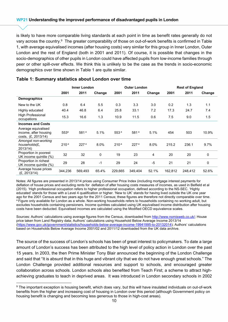
Whatever the cause, London is clearly very different from the rest of the country in ways that could influence trends in educational performance. Table 1 presents some more detailed background information about how Inner and Outer London differ from the rest of England and how these differences have evolved between 2001 and 2011 (years chosen to coincide with census years). This confirms that London has continued to experience faster immigration over the 2000s, with over 6% of individuals in Inner London new to the UK (in the past 2 years) in 2011 compared with around 3% in Outer London and 1% in the rest of England. The number of international immigrants has clearly risen since 2011, particularly in Inner London. We seek to account for this in our analysis by including detailed controls for ethnic background and language spoken at home in all our analysis, direct controls for immigration status for one particular cohort, and showing that trends are similar for those continuously present in England over time.

Table 1 further confirms that the socio–economic make-up of London is very different from the rest of England. Londoners are much more likely to be highly educated, work in professional occupations and have higher living standards on average. London also has higher levels of income inequality, with over 30% in the top UK income quintile in Inner London and nearly 30% in the bottom quintile. Our main data source only contains a binary measure of low-income (eligibility for free school meals) this means we cannot therefore control for all of the socio-economic differences between Londoners and the rest of England As a result, we focus exclusively on the educational performance of children from low-income families, specifically those eligible for free school meals or on out-of-work benefits. This group of families

6 Office for National Statistics, Annual Mid-year Population Estimates, 2013. 7 http://www.ons.gov.uk/ons/dcp171776_290558.pdf. 8 http://www.cityam.com/214488/sunday-times-rich-list-2015-london-has-more-billionaires-any-city-world

10


is likely to have more comparable living standards at each point in time as benefit rates generally do not vary across the country.9 The greater comparability of those on out-of-work benefits is confirmed in Table 1, with average equivalised incomes (after housing costs) very similar for this group in Inner London, Outer London and the rest of England (both in 2001 and 2011). Of course, it is possible that changes in the socio-demographics of other pupils in London could have affected pupils from low-income families through peer or other spill-over effects. We think this is unlikely to be the case as the trends in socio-economic demographics over time shown in Table 1 are quite similar.

Table 1: Summary statistics about London over time

Inner London Outer London Rest of England

2001 2011 Change 2001 2011 Change 2001 2011 Change

Demographics

New to the UK 0.8 6.4 5.5 0.3 3.3 3.0 0.2 1.3 1.1

Highly educated 40.4 46.8 6.4 25.8 33.1 7.2 17.3 24.7 7.4 High Professional occupations

15.3 16.6 1.3 10.9 11.5 0.6 7.5 9.0 1.5

Incomes and Costs Average equivalised income, after housing costs, (£, 2013/14)

553a 581 a 5.1% 553 a 581 a 5.1% 454 503 10.9%

Amongst non-working households(£, 2013/14)

210 a 227 a 8.0% 210 a 227 a 8.0% 215.2 236.1 9.7%

Proportion in poorest UK income quintile (%)

32 32 0 19 23 4 20 20 0

Proportion in richest UK income quintile (%)

29 28 -1 29 24 -5 21 21 0

Average house prices (£, 2013/14)

344,236 569,493 65.4% 229,665 349,404 52.1% 162,812 248,412 52.6%

Notes: All figures are presented in 2013/14 prices using Consumer Price Index (including mortgage interest payments for deflation of house prices and excluding rents for deflation of after housing costs measures of incomes, as used in Belfield et al (2015). ‘High professional occupation refers to higher professional occupation, defined according to the NS-SEC. ‘Highly educated’ stands for those with a Level 4 qualification or higher. ‘New to UK’ stands for having lived outside the UK one year ago for the 2001 Census and two years ago for the 2011 Census; these figures are therefore not directly comparable over time. a Figure only available for London as a whole. Non-working households refers to households containing no working adult, but excludes households containing pensioners. Income quintiles calculated using UK equivalised income distribution after housing costs have been deducted. Equivalised incomes are calculated using the Modified OECD equivalence scales. Sources: Authors’ calculations using average figures from the Census, downloaded from http://www.nomisweb.co.uk/; House price taken from Land Registry data; Authors’ calculations using Household Below Average Income 2013/14 (https://www.gov.uk/government/statistics/households-below-average-income-19941995-to-20132014); Authors’ calculations based on Households Below Average Income 2001/02 and 2011/12 downloaded from the UK data archive.

The source of the success of London’s schools has been of great interest to policymakers. To date a large amount of London’s success has been attributed to the high level of policy action in London over the past 15 years. In 2003, the then Prime Minister Tony Blair announced the beginning of the London Challenge and said that “It is absurd that in this huge and vibrant city that we do not have enough great schools.” The London Challenge provided additional resources and support to schools, and encouraged greater collaboration across schools. London schools also benefited from Teach First; a scheme to attract high-achieving graduates to teach in deprived areas. It was introduced in London secondary schools in 2002

9 The important exception is housing benefit, which does vary, but this will have insulated individuals on out-of-work benefits from the higher and increasing cost of housing in London over this period (although Government policy on housing benefit is changing and becoming less generous to those in high-cost areas).

11


and in London primary schools in 2011. Many of the first Academies were also set up in London in the early 2000s (Academies, like US Charter Schools, have significant levels of autonomy). London also received policy attention further back in time. The Excellence in Cities Programme (EiC) started in 1999 for secondary schools and combined extra resources with additional support. The programme was demonstrated to lead to improvements at age 14 but there is no evidence that this followed through to GCSE (McNally, Machin and Meghir, 2010). The National Literacy and Numeracy Strategies began with pilots in the late 1990s, with a disproportionate number of early adopters in Inner London. Studies have found positive effects of these national strategies on literacy, although the effects were generally found to be small (Machin and McNally, 2007) and the programme was eventually rolled out nationwide.

There are also other key differences in the schooling environment in London. There is a higher level of choice and competition compared with other areas of the country owing to the higher population density. However, most studies have found only weak effects of school competition in England (Gibbons et al, 2008). There are also higher levels of school funding to compensate for higher levels of teacher pay and other costs. The profile of teachers is different, with teachers being younger and less experienced, on average. However, Greaves et. al. (2014) show that most of these differences are longstanding. Furthermore, Greaves and Sibieta (2014) find no evidence of higher teacher pay impacting on educational attainment. There is no evidence to suggest that class sizes are lower in London10. Indeed, class sizes for Key Stage 2 (ages 7-11) are higher than all other regions, having not fallen over the 2000s. Between ages 11-16 class sizes in London followed the national downward trend11. Historically, the vast majority of Inner London local authorities were part of a single local education authority12 (the Inner London Local Education Authority), which was then abolished in 1990 and schools became the responsibility of individual London Boroughs.

In summary, the socio-economic and ethnic background of Londoners is very different from the rest of the England, with higher average incomes, higher house prices and higher levels of immigration being some of London’s hallmarks. This makes it hard to draw credible comparisons between London and the rest of England. However, low-income families with children inside and outside London have comparable living standards since the benefit system only varies with the cost of housing across the country. We therefore focus on the educational performance of this group over time. Although the socio-economic profile of Londoners is very different from families outside of London, there appears to be no evidence of differential trends over time, which makes it unlikely that the improvement in the relative performance of poorer pupils in London over time could be driven by spill-over or peer effects from the non-poor group. We account for the higher levels of immigration by including various controls for ethnic background, immigration status (in one dataset) and by looking the performance of those observed in England at the start and end of the period covered by our data.

3. Data

In order to better understand the improvement amongst poorer pupils in London, we make use of three different datasets: the National Pupil Database; the Youth Cohort Study and the Millennium Cohort Study. Each differs in terms of the years covered, sample size and available pupil characteristics. We now discuss their main advantages and disadvantages. Summary statistics from each dataset are shown in Table 2 (a),

10 https://www.gov.uk/government/uploads/system/uploads/attachment_data/file/183364/DFE-RR169.pdf 11 ibid 12 The exceptions being that Greenwich was not part of the Inner London Local Education Authority, but Haringey was.

12


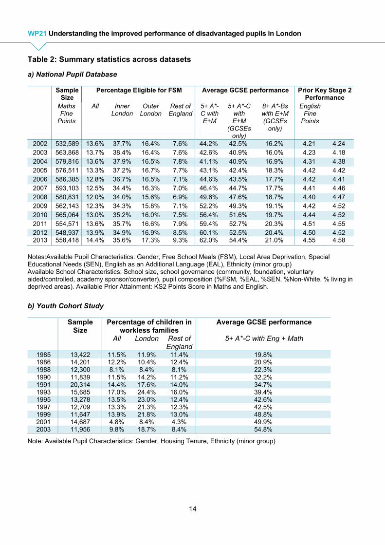
(b) and (c) for the National Pupil Database, Youth Cohort Study and Millennium Cohort Study, respectively. This shows the overall sample sizes, main measures of deprivation, average values of outcomes used and a list of available pupil and school characteristics. National Pupil Database Data

The main dataset we use is the National Pupil Database (NPD). The primary advantage of the NPD is that it is an administrative census of all children in the state-funded school system in England and thus has large sample sizes (varying from around 530,000 to 600,000 taking GCSE exams at age 16 each year between 2002 and 2013). It also contains information on pupil characteristics, including whether children are eligible and claiming free school meals (FSM). This is the main measure of socio-economic disadvantage available in the NPD and our analysis focuses on this group. Children are eligible for FSM if their families are eligible for a range of qualifying benefits. These are mainly out-of-work benefits, with the largest being income support and job-seekers allowance.13 However, to be recorded as eligible for FSM in the NPD, families must also make a claim for FSM. Nationally, around 13-14% of students taking their school exams at age 16 (GCSEs) were eligible and claiming for FSM over the 2000s. The proportion of children eligible for FSM is clearly higher in Inner London (35.6% in 2013) as compared with both Outer London (17.3%) and the rest of England (9.3%). However, these levels have been remarkably stable over time. The NPD allows us to examine a range of age 16 outcomes. We focus on four measures: Proportion of pupils gaining 5+ GCSEs (or equivalent) at A*-C (including Maths and English) Proportion of pupils gaining 5+ GCSEs (no equivalents) at A*-C (including Maths and English) The proportion getting 8 + GCSEs at A*-B (including Maths and English) Average point scores across pupils’ best eight GCSE results (standardised within year). The first outcome represents the standard benchmark of performance used for accessing post-compulsory schooling and is often a requirement of employers. As can be seen, there has been substantial growth in average performance on this measure, with the proportion achieving this level going up from 44% in 2002 to 62% by 2013. However, some of this growth relates to increased use of GCSE-equivalent vocational qualifications. The Wolf Review argued that these qualifications were mostly used to improve league table position and were likely to be of low value in the labour market (Wolf, 2011; McIntosh, 2006; Blanden and Macmillan, 2014). If we exclude these equivalents (our second measure of performance), then the growth in performance based on this measures has been much slower. Our third measure of performance seeks to examine very high levels of performance (achieving 8 or more GCSEs at A*-B, including English and Maths). This benchmark is achieved by a relatively small number of pupils each year (about 20% of pupils in 2013), but is likely to be an important indicator for whether pupils are then able to go to a high-status university after age 18. Our fourth outcome is a continuous measure of performance based on point scored across students’ best 8 GCSE or equivalents (standardised at the national level each year to have mean of zero and standard deviation of one). This outcome has the advantage of accounting for the achieved level of performance in each subject (rather than just a threshold measure). However, trends in average point score measures in the late 2000s are likely to have been heavily influence by the take-up of GCSE-equivalent vocational qualifications (which often counted as more than one and sometimes up to 5 GCSEs). This issue has led the government to recently reform the 13 Precise details available here (https://www.gov.uk/apply-free-school-meals).

13


secondary school accountability system and reduce the contribution of vocational qualifications to points score measures14. The main outcomes we use for performance at age 11 are Key Stage 2 fine point scores in both Maths and English15. Key Stage 2 tests are compulsory for all pupils in state-funded schools in England. They are marked externally and reported in school performance tables. Children are given a level between 3 and 6. However, the NPD also contains the raw marks and thus allows us to calculate a continuous point score measure. Table 2 shows the average values of the KS2 fine point score measures achieved by pupils taking GCSEs between 2002 and 2013 when they were aged 11 (i.e. between 1997 and 2008). In our main empirical analysis, we standardise these point score measures within year at the national level. We include missing dummies for when KS2 scores are missing (around 5% of cases in 2013), which is mostly the result of pupils being in private schools at age 11 or because pupils only moved to England after age 11. The NPD also allows us to control for a range of other characteristics such as detailed ethnicity16, whether pupils have special educational needs (SEN), whether pupils speak English as an Additional Language (EAL) and other area characteristics. The main disadvantages of this data are that it only allows us to examine age 16 results back to 2002 and background characteristics are relatively limited (e.g. there is no information on parental occupation education or activities with the child)17.

Youth Cohort Study The Youth Cohort Study (YCS) is a repeated survey of young people in the school system in the 1980s, 1990s and early 2000s (1985 to 2003). This allows us to understand trends in age 16 exams that pre-date the administrative information collected in the NPD. Similar to the NPD, it contains a range of different outcomes at age 16 and pupil characteristics. However, it does not include eligibility for FSM. We therefore instead use household worklessness as our measure of disadvantage in the YCS and focus on the performance of this group over time. This is only a minor disadvantage as eligibility for FSM over this time largely coincided with entitlement to out-of-work benefits. As we can see in Table 2 panel (b), the proportion classed as disadvantaged in the most recent years in the YCS (around 10-15% over the 1990s) is similar to that seen in the earlier years of the NPD (around 14% in the early 2000s)18.

14 https://www.gov.uk/government/speeches/reforming-the-accountability-system-for-secondary-schools 15 We do not use Key Stage 3 scores as a measure of prior attainment as these are tests taken at age 14, so could conceivably have been affected by secondary school quality between age 11 and 14. These test were also abolished from 2009 onwards. 16There are 10 ethnicities recorded, White British, White Other, Black African, Black Caribbean, Black Other, Asian Pakistani, Asian Bangladeshi, Asian Indian, Asian Chinese, Other Ethnicty. 17 Key Stage 1 teacher assessments are also available, but only for pupils taking Key Stage 2 from 2002 onwards, which misses the period of fast growth in Key Stage 2 scores in the late 1990s. Greaves et al (2014) make use of this data on Key Stage 1 scores and find that the London advantage is reduced by around one half after accounting for Key Stage 1 teacher assessments. However, the gap remains substantial and teacher assessments could be differences in subjective teacher judgements. 18 It should be noted that deprivations levels recorded in 2001 look unusual relative to earlier and later years. We therefore do not place any emphasis on results for 2001.

14


Table 2: Summary statistics across datasets

a) National Pupil Database

Sample Size

Percentage Eligible for FSM Average GCSE performance Prior Key Stage 2 Performance

Maths Fine

Points

All Inner London

Outer London

Rest of England

5+ A*-C with E+M

5+ A*-C with E+M

(GCSEs only)

8+ A*-Bs with E+M (GCSEs

only)

English Fine

Points

2002 532,589 13.6% 37.7% 16.4% 7.6% 44.2% 42.5% 16.2% 4.21 4.24 2003 563,868 13.7% 38.4% 16.4% 7.6% 42.6% 40.9% 16.0% 4.23 4.18 2004 579,816 13.6% 37.9% 16.5% 7.8% 41.1% 40.9% 16.9% 4.31 4.38 2005 576,511 13.3% 37.2% 16.7% 7.7% 43.1% 42.4% 18.3% 4.42 4.42 2006 586,385 12.8% 36.7% 16.5% 7.1% 44.6% 43.5% 17.7% 4.42 4.41 2007 593,103 12.5% 34.4% 16.3% 7.0% 46.4% 44.7% 17.7% 4.41 4.46 2008 580,831 12.0% 34.0% 15.6% 6.9% 49.6% 47.6% 18.7% 4.40 4.47 2009 562,143 12.3% 34.3% 15.8% 7.1% 52.2% 49.3% 19.1% 4.42 4.52 2010 565,064 13.0% 35.2% 16.0% 7.5% 56.4% 51.6% 19.7% 4.44 4.52 2011 554,571 13.6% 35.7% 16.6% 7.9% 59.4% 52.7% 20.3% 4.51 4.55 2012 548,937 13.9% 34.9% 16.9% 8.5% 60.1% 52.5% 20.4% 4.50 4.52 2013 558,418 14.4% 35.6% 17.3% 9.3% 62.0% 54.4% 21.0% 4.55 4.58

Notes:Available Pupil Characteristics: Gender, Free School Meals (FSM), Local Area Deprivation, Special Educational Needs (SEN), English as an Additional Language (EAL), Ethnicity (minor group) Available School Characteristics: School size, school governance (community, foundation, voluntary aided/controlled, academy sponsor/converter), pupil composition (%FSM, %EAL, %SEN, %Non-White, % living in deprived areas). Available Prior Attainment: KS2 Points Score in Maths and English.

b) Youth Cohort Study

Sample Size

Percentage of children in workless families

Average GCSE performance

All London Rest of England

5+ A*-C with Eng + Math

1985 13,422 11.5% 11.9% 11.4% 19.8% 1986 14,201 12.2% 10.4% 12.4% 20.9% 1988 12,300 8.1% 8.4% 8.1% 22.3% 1990 11,839 11.5% 14.2% 11.2% 32.2% 1991 20,314 14.4% 17.6% 14.0% 34.7% 1993 15,685 17.0% 24.4% 16.0% 39.4% 1995 13,278 13.5% 23.0% 12.4% 42.6% 1997 12,709 13.3% 21.3% 12.3% 42.5% 1999 11,647 13.9% 21.8% 13.0% 48.8% 2001 14,687 4.8% 8.4% 4.3% 49.9% 2003 11,956 9.8% 18.7% 8.4% 54.8%

Note: Available Pupil Characteristics: Gender, Housing Tenure, Ethnicity (minor group)

15


c) Millennium Cohort Study, English Sample

Sample Size

Percentage of children in families on JSA or income support

Average Test Score/ Performance in School Assessment (Standard deviation)

All London Inner London

Rest of England

Test Score School-based English

School-based Mathematics

Age 3 10097 23.5% 29.4% 17.2% 73.41 (17.51)

Age 5 9788 21.7% 28.6% 15.4% 108.06 (16.01)

25.04 (7.07)

20.26 (4.73)

Age 7 9499 25.4% 29.5% 17.1% 108.08 (30.14)

15.07 (4.06)

15.95 (3.79)

Age11 9266 19.4% 18.7% 14.8% 119.80 (16.56)

4.76 (.752)

4.79 (.817)

At any sweep

7910 47.3% 49.6% 36.4%

Notes:

Available Pupil Characteristics: Gender, age at tests, month of birth Local Area Deprivation, English as an Additional Language (EAL), ethnicity (minor group) Available School Characteristics: school governance (community, foundation, voluntary aided/controlled, academy sponsor/converter), faith school, single sex school. Available parental characteristics: mother and father’s education level, father present, mother and father’s occupational classification at each sweep, mother and father born in UK, if entered within last 10 years, information about activities done with children, religious activity and screen time. All analyses are weighted using the appropriate single-country longitudinal survey weight.

The main disadvantage of the YCS is the lower sample size, which ranges from about 11,000-20,000 pupils each year between 1985 and 2003, and naturally many fewer disadvantaged pupils. The number of available controls is also lower, with no information on Key Stage 2 tests (not in existence for most of the sample) and no information on school composition. As in the NPD, we use the proportion of children achieving 5 or more GCSE at A*-C (including English and Maths19) as our main outcome from the YCS.

Millennium Cohort Study

The Millennium Cohort Study (MCS) is a longitudinal survey of children born in 2000/2001. The first sweep sampled around 19,000 babies in the United Kingdom with the English and Welsh samples focused on those born in the academic year starting in September 2000. Importantly, the survey enables us to look at children’s skills and achievements in the pre-primary and primary years; so that we can observe if there is a positive London effect at earlier ages. Children are tested using instruments designed for the survey at every sweep so that we now have test scores from ages 3, 5, 7 and 11. The most comparable tests across sweeps (although not perfect as we shall discuss) focus on language and literacy. These are vocabulary tests at age 3 and 5, a reading test at age 7 and a measure of verbal reasoning at age 11. Information

19 This measure does not include GCSE-equivalents. However, as Table 2(a) makes clear, these only played a relatively small role in the early 2000s.

16


from school-based assessments are also matched into the data20, which means that we have information at age 5 from the Foundation Stage Profile, at age 7 at Key Stage 121 and at age 11 at Key Stage 222. The information from Key Stage 2 can be compared with our findings for a comparable cohort within the National Pupil Database; providing a useful cross-check. Table 2 panel (c) provides some basic statistics on the outcome measures available for children living in England at each sweep. In our analysis we use standardised measures with mean 0 and standard deviation 1 in the relevant sample. The survey is extremely rich with detailed information on the children’s socio-economic background in each survey, their parent’s behaviour, attitudes and activities with their children. Our aim is to use this additional information, unavailable in the NPD, to hold constant more of the factors which might make London’s children different. In our most detailed models we control for differences in parent’s social class and education level among our disadvantaged group of children in the relevant wave, as well as the presence of fathers. We are also able to include a range of controls for parental investments in the early years. Once children start school parents may adjust their behaviour in response; a positive school experience could lead to parents either increasing or decreasing their time spent on learning activities with children; or a change in educational aspirations. To prevent our results being affected by this endogeneity we therefore focus on time spent undertaking a range of learning activities at age 3 and 523. While we can never rule out unobservable differences between children in and outside of London we feel that the measures provide a comprehensive picture of education-related activities in families; they have substantial overlaps with measures of the Home Learning Environment that have been shown to be so important to children’s educational development (Melhuish et al 2008, Goodman and Gregg, 2010). Another particularly interesting aspect of the MCS is the ability to look in more detail at the migration status of parents; the MCS tells us whether they were born in the UK and if not, when they arrived. However, it should be noted that the MCS does not include children who migrate to the UK after they are born. If this group were particularly important in generating the London advantage at age 11 then the MCS results should understate it compared to the NPD. We show this is unlikely to be the case. Religious observance is also higher among migrant groups and we thus additionally control for (self-reported) religious observance. The MCS does include information about eligibility for Free School Meals, however this is not available at ages 3 and 5. We instead focus on benefit receipt which is strongly related to eligibility; receipt of Income Support or Job Seekers Allowance (as noted earlier, the criteria for FSM are slightly wider, but these are the two main qualifying benefits). Table 1 panel (c) shows the share of children in each sweep who fall into

20 Available under special license 21 The Key Stage 1 results are only provided in levels, and therefore have less continuous variation than the other outcome measures we use. Fortunately, outcomes at age 7 are of less interest than changes between ages 5 and 11. 22 These tests impose quite different incentives on schools. Foundation Stage Profiles and Key Stage 1 are teacher assessed and are not generally used to compare school performance (either by parents or policymakers). Key Stage 2, on the other hand, is externally assessed and represents the main performance measure for primary schools in league tables and accountability regimes. 23 At age 3, this comprises time spent with children doing six activities at age 3 (reading to child, helping with numbers, drawing, singing etc) as well as frequency of visiting the library. At age 5 more detail is available. The information on one-to-one activities is collapsed into an index and information is separately added on the number of cultural visits, frequency of religious activities, help with reading, writing and maths and time spent on the computer and watching television. Information on frequency of visits to the library is available again at this age.

17


this group across the different areas of England; this is 20-25% across all of London, closer to 30% in Inner London and 15-17% in each sweep for the rest of the country. This seems broadly in line with the NPD; particularly in light of the fact that not everyone who is on eligible benefits will apply for Free School Meals. In order to ensure sufficient sample sizes we consider children to be disadvantaged who have been in families claiming benefits at age 3, 5, 7 or 11; we can see that a larger share falls into this group; almost half of children in Inner London and 36% of children across the rest of England. Our MCS sample therefore covers a larger share of children who are on average are likely to be slightly less disadvantaged compared with the NPD sample. Note that our results are based on a limited group of children who have information at ages 3, 5, 7 and 11; just under 8000, compared with 10,000 in the survey at age 3. We must therefore worry about the impact of attrition and survey non-response for our findings. In addition, there is a large drop in the proportion of children on benefits at 11 in Inner London which is not there for any other group; this is likely a consequence of the small sample. The combined impacts of attrition and small sample sizes mean we will need to be more cautious in our interpretation of the MCS compared with the population results from the NPD. We therefore avoid showing results for Inner London and focus on London as a whole instead. Our results from here on in are based on the sample of children who are available at all sweeps and are appropriately weighted using the age 11 longitudinal sample weights; this is a somewhat advantaged subsample of the full MCS (as shown in Appendix Tables 1 and 2). Results for the maximum sample at each sweep are available by request and are qualitatively very similar.

4. Basic Empirical Facts

We start by providing some basic empirical facts about the improved performance of disadvantaged pupils in London over time. This already provides us with significant insight into the likely factors driving the higher level and improved performance of disadvantaged pupils in London over time. Fact #1 – The performance of disadvantaged pupils in London in exams at age 16 has improved substantially, starting from the mid-1990s onwards Figure 2 show the raw difference between London and rest of England in terms of the performance of disadvantaged pupils (those eligible for free school meals in the NPD or those in workless households in the YCS) in exams at age 16 (whether they achieved the standard benchmark of achieving 5 or more GCSEs or their equivalent at A*-C, inclusive of English and Maths). This is shown for years from 1985 to 2003 based on the YCS and for 2002 through to 2013 based on the NPD (the higher sample sizes in the latter allows us to further split the difference by inner and Outer London). From the mid-1980s through to the mid-1990s, disadvantaged pupils performed at about the same level or worse as compared with disadvantaged pupils elsewhere in England. Starting from the mid-1990s onwards, the performance of disadvantaged pupils in London improved dramatically relative to elsewhere in England. In 1995, disadvantaged pupils were about 4 percentage points less likely to achieve the standard benchmark at age 16. By 2003, they were 5 percentage points more likely. These improvements continued throughout the 2000s and were even more dramatic for pupils in Inner London than those in Outer London. By 2013, disadvantaged pupils in Inner London were 19 percentage points more likely to

18


achieve 5 or more GCSEs at A*-C (including English and Maths) as compared with disadvantaged pupils outside of London, and disadvantaged pupils in Outer London were 13 percentage points more likely. Although we are using different measures of disadvantage across the two datasets, it is reassuring to see that the growth in the performance of disadvantaged pupils can be seen in both datasets and that the London effect is similar in the years when the datasets overlap each other in the early 2000s. Figure 2: Estimated difference in proportion of disadvantaged pupils achieving 5+ GCSEs at A*-C (including English and Maths) between London and the rest of England

Sources: Authors’ calculations using Youth Cohort Study (1985 to 2003); National Pupil Database (2002 to 2013).

Notes: YCS uses household worklessness as measure of disadvantage, NPD eligibility for free school meals.

These improvements are not confined to a single outcome. Table 3 shows the Inner and Outer London effects for disadvantaged pupils across a range of measures of achievement (selected years between 2002 and 2013). The first column repeats the results from Figure 1. Column (2) shows that the improvements in performance in Inner London are slightly larger if we exclude these low-value equivalent qualifications, which implies that London schools were less likely to rely on them (which has also been shown by Burgess (2014)). Column (3) shows that the improvements in London on a measure of high performance is even more dramatic (rising from a raw difference of 2.6 percentage points in 2002 to 9.2 percentage points in 2013 for Inner London). This rise in the raw gap now makes disadvantaged pupils in Inner London more than twice as likely to achieve this higher benchmark as similar pupils outside of London. Rather than relying on whether pupils achieved a given threshold, the final column uses a measure of total points scored across all qualifications (average points scored across best 8 qualifications and standardised at the national level). Here, we see a higher level of performance for disadvantaged pupils in London, as well as growth between 2002 and 2009. However, performance tails off slightly after 2009. It is unclear

‐0.1

‐0.05

0

0.05

0.1

0.15

0.2

Pro

bab

ility

of

ach

ievi

ng

5+

GC

SE

s at

A*-

C

(in

clu

din

g E

ng

lish

an

d M

ath

s) r

elat

ive

to r

est

of

En

gla

nd

Inner London - Raw (NPD) Outer London - Raw (NPD) London - Raw (YCS)

19


what is driving this reduced London effect after 2009, but it could relate to the greater use of vocational qualifications by schools outside of London. Table 3: Raw London effects for 2002, 2005, 2009, 2013 for three different measures of GCSE performance amongst children eligible for Free School Meals

5+ A*-C with Eng + Math

5+ A*-C with Eng + Math (GCSEs only)

8+ Bs with Eng + Math (GCSEs only)

Capped Points Score (Std)

Inner Outer Inner Outer Inner Outer Inner Outer

2002 0.062*** 0.051*** 0.063*** 0.054*** 0.024*** 0.022*** 0.307*** 0.229*** [0.009] [0.009] [0.009] [0.008] [0.003] [0.003] [0.033] [0.029]

2005 0.101*** 0.071*** 0.100*** 0.072*** 0.035*** 0.026*** 0.432*** 0.282*** [0.010] [0.008] [0.010] [0.008] [0.005] [0.003] [0.033] [0.028]

2009 0.160*** 0.102*** 0.155*** 0.111*** 0.048*** 0.036*** 0.422*** 0.300*** [0.010] [0.009] [0.009] [0.009] [0.004] [0.004] [0.032] [0.026]

2013 0.185*** 0.126*** 0.206*** 0.151*** 0.073*** 0.061*** 0.342*** 0.246*** [0.012] [0.009] [0.010] [0.009] [0.005] [0.004] [0.036] [0.029]

Notes: Differences relate to higher performance of pupils eligible for FSM in inner and outer London compared with the rest of England. GCSE capped points score represents average points scored across pupils’ best eight GCSE or equivalent qualifications (A*=58, A=52, B=46, C=40...,G=16,U=0) and is expressed in standardised terms (i.e. mean = 0, SD = 1 amongst the whole cohort each year).

Two potential objections to these results are that this could reflect a general large city effect (rather than something specific to London) or that the results could be driven by changing mobility of pupils over time (either mobility within England or new pupils joining from outside England). On the first point, other large cities such as Birmingham and Manchester have also seen improvements in the performance of disadvantaged pupils. However, as shown in Greaves et al (2014) these improvements have not been anywhere near as dramatic as is the case for Inner London and they are not sustained into improved post-16 outcomes (as is the case for disadvantaged pupils in London). On the second point, Figure 3 suggests that differential mobility is unlikely to form a significant explanation for the growth of the London Effect. One can observe identical trends in the relative performance of disadvantaged pupils in Inner London if one restricts the sample to those observed in England at ages 11 and 16 (always England) and if one drops pupils who moved between London and the rest of England between ages 11 and 16 (always London). Disadvantaged pupils in London, particularly those in Inner London, have therefore seen a rapid improvement in results starting from the mid-1990s and are now achieving much higher results at age 16 than disadvantaged pupils outside of London. This can be seen across a range of measures of performance at age 16, particularly those that focus on high-quality qualifications or high-levels of performance. The one exception is the slight tailing off of performance after 2009 as measured by the average points score. One observes identical trends if we restrict the sample to those observed in England at both ages 11 and 16 if we exclude movers between London and the rest of England

20


Figure 3: Estimated difference in proportion of disadvantaged pupils achieving 5+ GCSEs at A*-C (including English and Maths) between Inner London and the rest of England, various samples over time

Sources: National Pupil Database (2002 to 2013) Notes: Always London excludes pupils who moved to or from London between ages 11 and 16; Always England means pupils was observed as attending a state-funded school in England at ages 11 and 16.

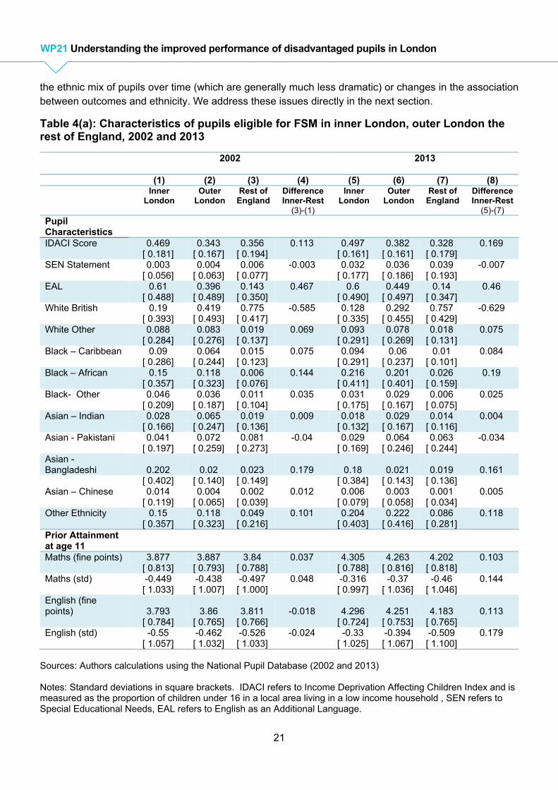
Fact #2 - The characteristics of disadvantaged pupils in London are very different from those outside of London, and in ways that matter for pupil attainment

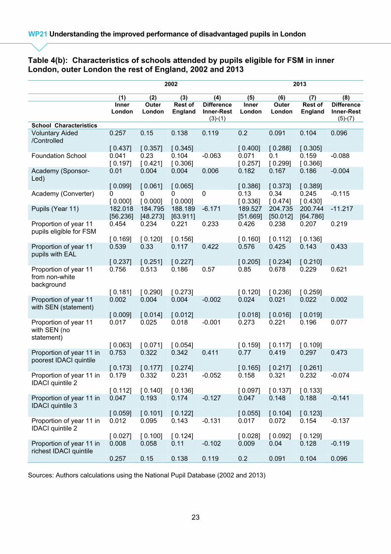
Table 4(a) shows the characteristics of disadvantaged pupils across Inner London, Outer London and the rest of England for 2002 and 2013, as well as the difference between Inner London and the rest of England. Table 4(b) shows the same set of statistics for the characteristics of schools attended by disadvantaged pupils.

What is immediately clear is that the characteristics of disadvantaged pupils in London are very different from those outside of London, with the differences being particularly large for Inner London. Disadvantaged pupils in Inner London are much less likely to come from a White-British background (13% in Inner London in 2013 as compared with 76% outside of London) and much more likely to come from other ethnic backgrounds. Indeed, in 2013, White-British pupils were a minority amongst disadvantaged pupils in Inner London with the largest ethnic group being pupils from Black-African backgrounds (22%). Pupils in Inner London are also much more likely to speak English as an Additional Language (EAL), with 60% of disadvantaged pupils in Inner London with EAL in 2013 as compared with 14% outside of London24. These differences are important as previous work has shown that many ethnic minorities tend to outperform White-British pupils and also have different educational trajectories, often being behind at the start of school before then overtaking White-British pupils by age 16 or earlier (Dustmann, Machin and Schonberg, 2010, Wilson, Burgess and Briggs, 2011). The greater concentration of ethnic minorities in Inner London may thus form an important explanation for the higher level of performance in London (as is argued by Burgess, 2014). However, to explain the growth in performance, we would need to see large changes in

24 A high proportion of pupils in other large cities also come from ethnic minority backgrounds. However, this is still less than the figures for Inner London. For instance, Greaves et al (2014) show that 60% of pupils in Birmingham and 50% of pupils in Manchester come from ethnic backgrounds other than White-British.

0%

5%

10%

15%

20%

25%

2002 2003 2004 2005 2006 2007 2008 2009 2010 2011 2012 2013Per

cen

atg

e ac

hie

vin

g 5

+ G

CS

Es

at

A*-

C (

incl

ud

ing

En

gli

sh a

nd

Mat

hs)

re

lati

ve t

o r

est

of

En

gla

nd

Inner London - FSM Inner London - FSM & Always London Inner London - FSM & Always England

21


the ethnic mix of pupils over time (which are generally much less dramatic) or changes in the association between outcomes and ethnicity. We address these issues directly in the next section.

Table 4(a): Characteristics of pupils eligible for FSM in inner London, outer London the rest of England, 2002 and 2013

2002 2013

(1) (2) (3) (4) (5) (6) (7) (8) Inner

London Outer

London Rest of

England DifferenceInner-Rest

(3)-(1)

Inner London

Outer London

Rest of England

DifferenceInner-Rest

(5)-(7) Pupil Characteristics

IDACI Score 0.469 0.343 0.356 0.113 0.497 0.382 0.328 0.169 [ 0.181] [ 0.167] [ 0.194] [ 0.161] [ 0.161] [ 0.179] SEN Statement 0.003 0.004 0.006 -0.003 0.032 0.036 0.039 -0.007 [ 0.056] [ 0.063] [ 0.077] [ 0.177] [ 0.186] [ 0.193] EAL 0.61 0.396 0.143 0.467 0.6 0.449 0.14 0.46 [ 0.488] [ 0.489] [ 0.350] [ 0.490] [ 0.497] [ 0.347] White British 0.19 0.419 0.775 -0.585 0.128 0.292 0.757 -0.629 [ 0.393] [ 0.493] [ 0.417] [ 0.335] [ 0.455] [ 0.429] White Other 0.088 0.083 0.019 0.069 0.093 0.078 0.018 0.075 [ 0.284] [ 0.276] [ 0.137] [ 0.291] [ 0.269] [ 0.131] Black – Caribbean 0.09 0.064 0.015 0.075 0.094 0.06 0.01 0.084 [ 0.286] [ 0.244] [ 0.123] [ 0.291] [ 0.237] [ 0.101] Black – African 0.15 0.118 0.006 0.144 0.216 0.201 0.026 0.19 [ 0.357] [ 0.323] [ 0.076] [ 0.411] [ 0.401] [ 0.159] Black- Other 0.046 0.036 0.011 0.035 0.031 0.029 0.006 0.025 [ 0.209] [ 0.187] [ 0.104] [ 0.175] [ 0.167] [ 0.075] Asian – Indian 0.028 0.065 0.019 0.009 0.018 0.029 0.014 0.004 [ 0.166] [ 0.247] [ 0.136] [ 0.132] [ 0.167] [ 0.116] Asian - Pakistani 0.041 0.072 0.081 -0.04 0.029 0.064 0.063 -0.034 [ 0.197] [ 0.259] [ 0.273] [ 0.169] [ 0.246] [ 0.244] Asian - Bangladeshi 0.202 0.02 0.023 0.179 0.18 0.021 0.019 0.161 [ 0.402] [ 0.140] [ 0.149] [ 0.384] [ 0.143] [ 0.136] Asian – Chinese 0.014 0.004 0.002 0.012 0.006 0.003 0.001 0.005 [ 0.119] [ 0.065] [ 0.039] [ 0.079] [ 0.058] [ 0.034] Other Ethnicity 0.15 0.118 0.049 0.101 0.204 0.222 0.086 0.118 [ 0.357] [ 0.323] [ 0.216] [ 0.403] [ 0.416] [ 0.281] Prior Attainment at age 11 Maths (fine points) 3.877 3.887 3.84 0.037 4.305 4.263 4.202 0.103 [ 0.813] [ 0.793] [ 0.788] [ 0.788] [ 0.816] [ 0.818] Maths (std) -0.449 -0.438 -0.497 0.048 -0.316 -0.37 -0.46 0.144 [ 1.033] [ 1.007] [ 1.000] [ 0.997] [ 1.036] [ 1.046] English (fine points) 3.793 3.86 3.811 -0.018 4.296 4.251 4.183 0.113 [ 0.784] [ 0.765] [ 0.766] [ 0.724] [ 0.753] [ 0.765] English (std) -0.55 -0.462 -0.526 -0.024 -0.33 -0.394 -0.509 0.179 [ 1.057] [ 1.032] [ 1.033] [ 1.025] [ 1.067] [ 1.100]

Sources: Authors calculations using the National Pupil Database (2002 and 2013) Notes: Standard deviations in square brackets. IDACI refers to Income Deprivation Affecting Children Index and is measured as the proportion of children under 16 in a local area living in a low income household , SEN refers to Special Educational Needs, EAL refers to English as an Additional Language.

22


The same is true across other margins where disadvantaged pupils in Inner London differ from those outside of London. Disadvantaged pupils in Inner London are more likely than those outside of London to live in a deprived neighbourhood, more likely to attend voluntary aided/controlled schools (mostly Church run), less likely to attend foundation schools (which have more control over their own affairs), as well as have a peer group that contains more disadvantaged pupils, more pupils from an ethnic minority and who speak English as an Additional Language. However, crucially, many of these differences are longstanding and have not changed substantially over time.

One large change over this period is the increasing numbers of schools that are Academies, either set up as new schools in the 2000s (sponsor-led) or schools that converted to Academy status after 2010. By 2013, pupils in Inner London were less likely to attend a converter Academy, but there was no great difference in the proportion of disadvantaged pupils attending sponsor-led Academies between Inner London and rest of England. This distinction is important as existing work shows that the early sponsor-led Academies have had a positive effect on pupil attainment (Machin and Vernoit, 2011), but there is no clear evidence linking more recent converter Academies to subsequent positive effects on pupil attainment.

Appendix Table 1 demonstrates that London children are also different in the MCS cohort; these children were born five years later than the last GCSE cohort we observe and will take their GCSEs in 2017. 40% of children in London speak English as an additional language, compared with 10% in the rest of England25. The MCS also gives additional information on parental characteristics not available in the NPD; not surprisingly there is a large difference in migration status with 60% of mothers in London born in the UK compared with 93% outside. In contrast there is little difference in parental education and occupation among disadvantaged children inside and outside the capital, confirming our choice to restrict our analysis to disadvantaged children, in part to minimise heterogeneity among the group of children in question.

Overall, these results suggest that, as shown by Burgess (2014), some of the London advantage observed may be accounted for by the characteristics of London children. However, since many of these differences have remained largely constant over time, it would need to be the case that their impact on performance had changed dramatically; a hypothesis we can test in the next section.

25 The slightly lower proportions here compared with the NPD are most likely because the MCS does not include children born outside the UK.

23


Table 4(b): Characteristics of schools attended by pupils eligible for FSM in inner London, outer London the rest of England, 2002 and 2013

2002 2013

(1) (2) (3) (4) (5) (6) (7) (8) Inner

London Outer

London Rest of

EnglandDifferenceInner-Rest

(3)-(1)

Inner London

Outer London

Rest of England

DifferenceInner-Rest

(5)-(7) School Characteristics Voluntary Aided /Controlled

0.257 0.15 0.138 0.119 0.2 0.091 0.104 0.096

[ 0.437] [ 0.357] [ 0.345] [ 0.400] [ 0.288] [ 0.305] Foundation School 0.041 0.23 0.104 -0.063 0.071 0.1 0.159 -0.088 [ 0.197] [ 0.421] [ 0.306] [ 0.257] [ 0.299] [ 0.366] Academy (Sponsor-Led)

0.01 0.004 0.004 0.006 0.182 0.167 0.186 -0.004

[ 0.099] [ 0.061] [ 0.065] [ 0.386] [ 0.373] [ 0.389] Academy (Converter) 0 0 0 0 0.13 0.34 0.245 -0.115 [ 0.000] [ 0.000] [ 0.000] [ 0.336] [ 0.474] [ 0.430] Pupils (Year 11) 182.018 184.795 188.189 -6.171 189.527 204.735 200.744 -11.217 [56.236] [48.273] [63.911] [51.669] [50.012] [64.786] Proportion of year 11 pupils eligible for FSM

0.454 0.234 0.221 0.233 0.426 0.238 0.207 0.219

[ 0.169] [ 0.120] [ 0.156] [ 0.160] [ 0.112] [ 0.136] Proportion of year 11 pupils with EAL

0.539 0.33 0.117 0.422 0.576 0.425 0.143 0.433

[ 0.237] [ 0.251] [ 0.227] [ 0.205] [ 0.234] [ 0.210] Proportion of year 11 from non-white background

0.756 0.513 0.186 0.57 0.85 0.678 0.229 0.621

[ 0.181] [ 0.290] [ 0.273] [ 0.120] [ 0.236] [ 0.259] Proportion of year 11 with SEN (statement)

0.002 0.004 0.004 -0.002 0.024 0.021 0.022 0.002

[ 0.009] [ 0.014] [ 0.012] [ 0.018] [ 0.016] [ 0.019] Proportion of year 11 with SEN (no statement)

0.017 0.025 0.018 -0.001 0.273 0.221 0.196 0.077

[ 0.063] [ 0.071] [ 0.054] [ 0.159] [ 0.117] [ 0.109] Proportion of year 11 in poorest IDACI quintile

0.753 0.322 0.342 0.411 0.77 0.419 0.297 0.473

[ 0.173] [ 0.177] [ 0.274] [ 0.165] [ 0.217] [ 0.261] Proportion of year 11 in IDACI quintile 2

0.179 0.332 0.231 -0.052 0.158 0.321 0.232 -0.074


0.047 0.193 0.174 -0.127 0.047 0.148 0.188 -0.141


0.012 0.095 0.143 -0.131 0.017 0.072 0.154 -0.137

[ 0.027] [ 0.100] [ 0.124] [ 0.028] [ 0.092] [ 0.129] Proportion of year 11 in richest IDACI quintile

0.008 0.058 0.11 -0.102 0.009 0.04 0.128 -0.119

0.257 0.15 0.138 0.119 0.2 0.091 0.104 0.096 Sources: Authors calculations using the National Pupil Database (2002 and 2013)

24


Notes: Standard deviations in square brackets. IDACI refers to Income Deprivation Affecting Children Index and is measured as the proportion of children under 16 in a local area living in a low income household , SEN refers to Special Educational Needs, EAL refers to English as an Additional Language.

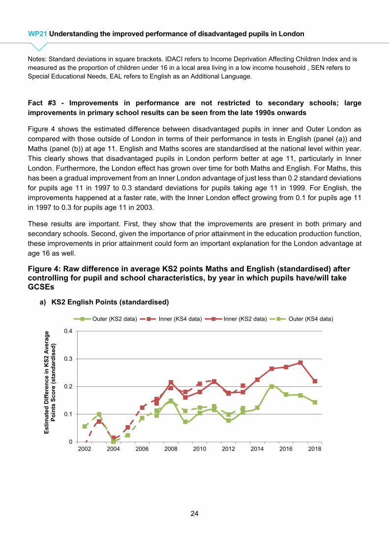
Fact #3 - Improvements in performance are not restricted to secondary schools; large improvements in primary school results can be seen from the late 1990s onwards

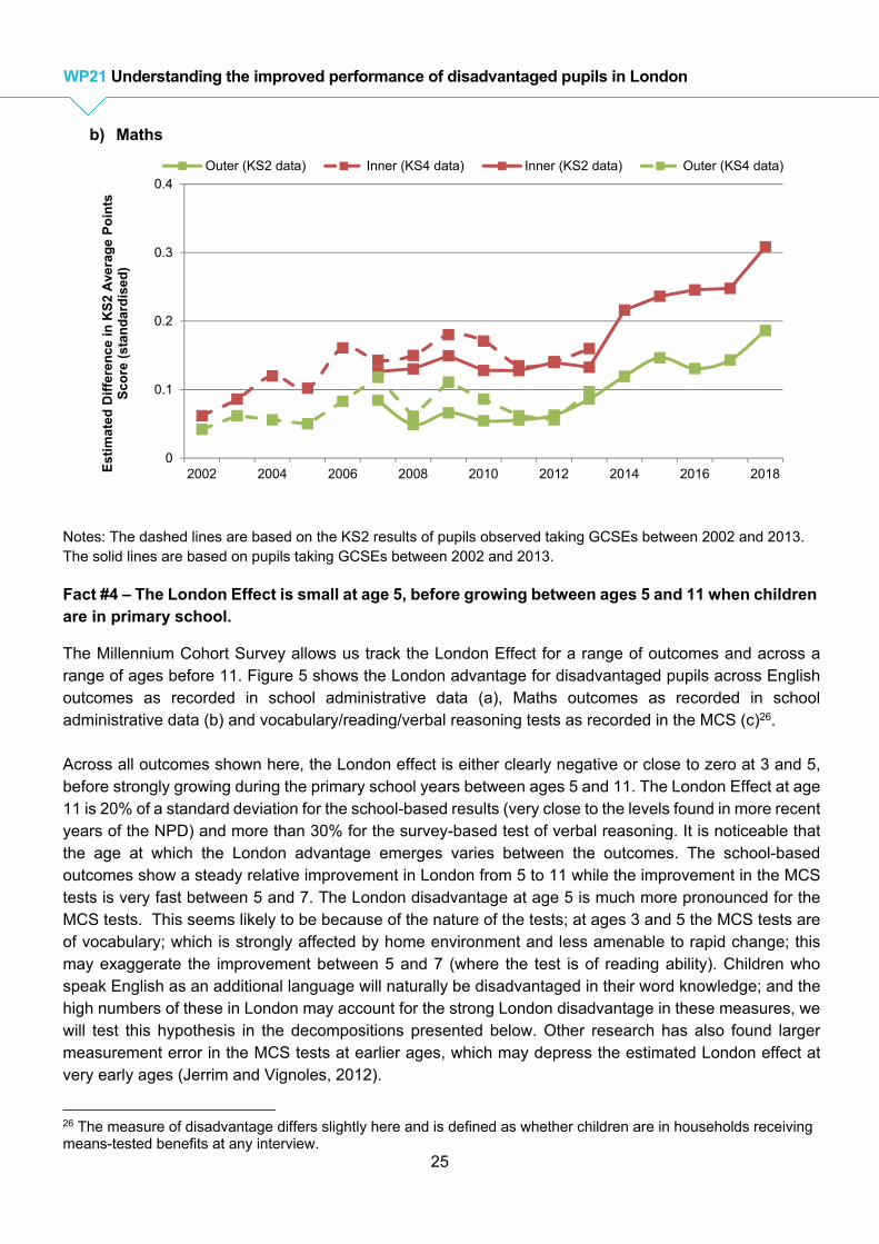
Figure 4 shows the estimated difference between disadvantaged pupils in inner and Outer London as compared with those outside of London in terms of their performance in tests in English (panel (a)) and Maths (panel (b)) at age 11. English and Maths scores are standardised at the national level within year. This clearly shows that disadvantaged pupils in London perform better at age 11, particularly in Inner London. Furthermore, the London effect has grown over time for both Maths and English. For Maths, this has been a gradual improvement from an Inner London advantage of just less than 0.2 standard deviations for pupils age 11 in 1997 to 0.3 standard deviations for pupils taking age 11 in 1999. For English, the improvements happened at a faster rate, with the Inner London effect growing from 0.1 for pupils age 11 in 1997 to 0.3 for pupils age 11 in 2003.

These results are important. First, they show that the improvements are present in both primary and secondary schools. Second, given the importance of prior attainment in the education production function, these improvements in prior attainment could form an important explanation for the London advantage at age 16 as well.

Figure 4: Raw difference in average KS2 points Maths and English (standardised) after controlling for pupil and school characteristics, by year in which pupils have/will take GCSEs

a) KS2 English Points (standardised)

0

0.1

0.2

0.3

0.4

2002 2004 2006 2008 2010 2012 2014 2016 2018

Est

imat

ed D

iffe

ren

ce i

n K

S2

Ave

rag

e P

oin

ts S

core

(st

and

ard

ised

)

Outer (KS2 data) Inner (KS4 data) Inner (KS2 data) Outer (KS4 data)

25


b) Maths

Notes: The dashed lines are based on the KS2 results of pupils observed taking GCSEs between 2002 and 2013. The solid lines are based on pupils taking GCSEs between 2002 and 2013.

Fact #4 – The London Effect is small at age 5, before growing between ages 5 and 11 when children are in primary school.

The Millennium Cohort Survey allows us track the London Effect for a range of outcomes and across a range of ages before 11. Figure 5 shows the London advantage for disadvantaged pupils across English outcomes as recorded in school administrative data (a), Maths outcomes as recorded in school administrative data (b) and vocabulary/reading/verbal reasoning tests as recorded in the MCS (c)26. Across all outcomes shown here, the London effect is either clearly negative or close to zero at 3 and 5, before strongly growing during the primary school years between ages 5 and 11. The London Effect at age 11 is 20% of a standard deviation for the school-based results (very close to the levels found in more recent years of the NPD) and more than 30% for the survey-based test of verbal reasoning. It is noticeable that the age at which the London advantage emerges varies between the outcomes. The school-based outcomes show a steady relative improvement in London from 5 to 11 while the improvement in the MCS tests is very fast between 5 and 7. The London disadvantage at age 5 is much more pronounced for the MCS tests. This seems likely to be because of the nature of the tests; at ages 3 and 5 the MCS tests are of vocabulary; which is strongly affected by home environment and less amenable to rapid change; this may exaggerate the improvement between 5 and 7 (where the test is of reading ability). Children who speak English as an additional language will naturally be disadvantaged in their word knowledge; and the high numbers of these in London may account for the strong London disadvantage in these measures, we will test this hypothesis in the decompositions presented below. Other research has also found larger measurement error in the MCS tests at earlier ages, which may depress the estimated London effect at very early ages (Jerrim and Vignoles, 2012).

26 The measure of disadvantage differs slightly here and is defined as whether children are in households receiving means-tested benefits at any interview.

0

0.1

0.2

0.3

0.4

2002 2004 2006 2008 2010 2012 2014 2016 2018Est

imat

ed D

iffe

ren

ce i

n K

S2

Ave

rag

e P

oin

ts

Sco

re (

stan

dar

dis

ed)

Outer (KS2 data) Inner (KS4 data) Inner (KS2 data) Outer (KS4 data)

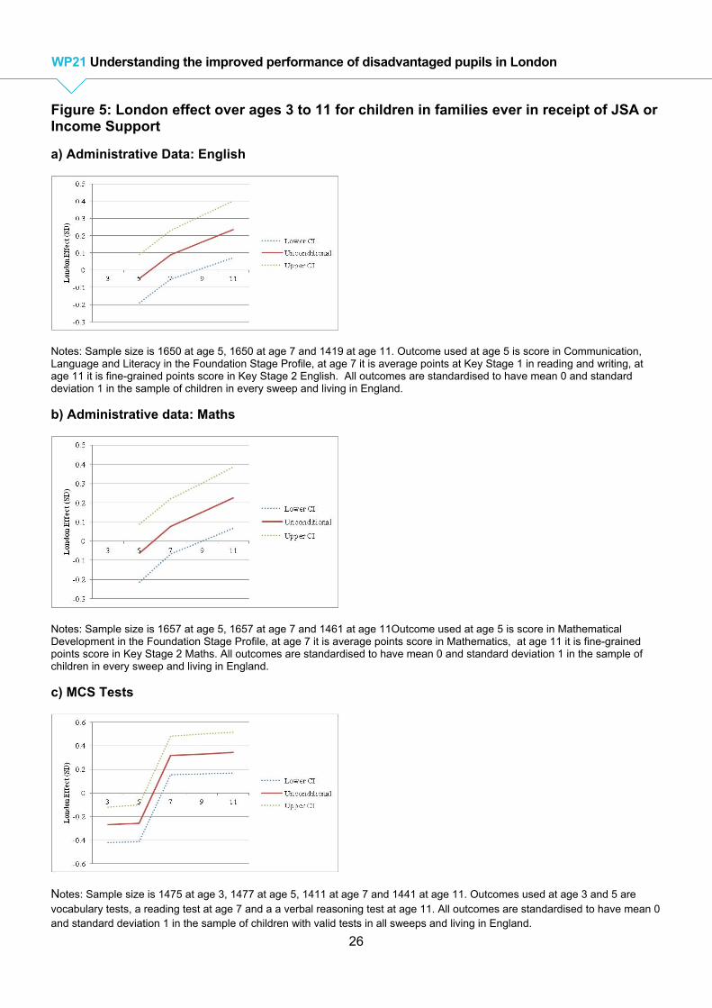
26


Figure 5: London effect over ages 3 to 11 for children in families ever in receipt of JSA or Income Support

a) Administrative Data: English

Notes: Sample size is 1650 at age 5, 1650 at age 7 and 1419 at age 11. Outcome used at age 5 is score in Communication, Language and Literacy in the Foundation Stage Profile, at age 7 it is average points at Key Stage 1 in reading and writing, at age 11 it is fine-grained points score in Key Stage 2 English. All outcomes are standardised to have mean 0 and standard deviation 1 in the sample of children in every sweep and living in England.

b) Administrative data: Maths

Notes: Sample size is 1657 at age 5, 1657 at age 7 and 1461 at age 11Outcome used at age 5 is score in Mathematical Development in the Foundation Stage Profile, at age 7 it is average points score in Mathematics, at age 11 it is fine-grained points score in Key Stage 2 Maths. All outcomes are standardised to have mean 0 and standard deviation 1 in the sample of children in every sweep and living in England.

c) MCS Tests

Notes: Sample size is 1475 at age 3, 1477 at age 5, 1411 at age 7 and 1441 at age 11. Outcomes used at age 3 and 5 are vocabulary tests, a reading test at age 7 and a a verbal reasoning test at age 11. All outcomes are standardised to have mean 0 and standard deviation 1 in the sample of children with valid tests in all sweeps and living in England.

27


Overall, these results indicate that Londoners do not start school with an advantage; the London effect develops during the school years between 5 and 11.

Summary and implications of the basic facts These basic facts illustrate the dramatic improvements in the performance of disadvantaged pupils in London over time. In addition, they already provide some clear indications as to the likely explanations for the London Effect, and also suggest which factors are likely to be less important. First, the improvements stretch back to the mid-1990s which rules out several popular explanations: the London Challenge for secondary schools started in 2004, Teach First from the early 2000s onwards and the Academies programme for secondary schools from the early 2000s onwards. Second, there are very clear differences in the characteristics of disadvantaged pupils in London as compared with the rest of England, particularly in terms of the ethnic mix. Although these differences are longstanding, so are unlikely to explain the growth in performance, it is important to account for the role in both child and parent characteristics in explaining the London Effect. In the next section we will use a robust decomposition technique to analyse this aspect. Third, the improvements also occurred in primary schools; providing further evidence that a focus on secondary school interventions will miss part of the picture. It is not that we think these policies had no effect, but their timing and focus suggests that they cannot be the only explanation for the London Effect for disadvantaged pupils. Finally, we have shown that disadvantaged pupils generally start primary school at age 5 at a similar level or behind their peers elsewhere in England. The London advantage then generally grows from the period they start school at age 5 through to age 11. Disadvantaged pupils at age 5 in London also share similar observable socio-economic characteristics to those outside of London, despite the dramatic differences in ethnicity. The similarity of outcomes and observable socio-economic characteristics at age 5 makes it less likely that the London effect is driven by unobserved heterogeneity or differences in parental investments, and more likely to result from contact with schools. In the next sections we test these hypotheses directly.

28


5. Decomposition Analysis

a) Empirical Framework

Our basic facts have revealed that observable characteristics are quite different for disadvantaged pupils in London as compared with those in the rest of England, and may explain a large part of the London advantage. We expect a role for ethnicity and prior attainment in leading to higher attainment for Londoners at secondary level; and it is possible that the rich data on parental characteristics and attitudes can explain the strong progress through the primary years observed in the MCS. In this section we outline an empirical method for decomposing the precise role of pupil, school and family characteristics.

As a starting point, we assume a simple education production function. Following Todd and Wolpin (2003) and Hanushek and Rivkin (2006), let us assume that the educational attainment of pupil (i) at school (s) at time (t) is a function of family background ( , , ), parental investments up to time t ( , , ), school characteristics up to time t ( , , ), prior achievement ( , , ); and pupil ability ( . Family background could include such factors as ethnicity and other aspects of parental background. Parental investments can include a wide variety of investments throughout childhood, such as the early home learning environment or help with homework. School characteristics could include school type, the peer group within the school and the overall level of school quality.

, , , , , , , , ,, , (1)

Let us further assume that the production function shown in (1) is linear in form. We can then follow the simple methodology outlined in Gelbach (2014) to decompose the difference between the average performance of disadvantaged pupils in London as compared with the rest of England.

First, in equation (2a), we estimate the raw London gap in the outcome of interest at time (t) as . Equation (2b) then estimates the London gap after controlling for pupil and school characteristics, and prior attainment ( ).

, . (2a)

, . , (2b)

One can then decompose the difference ( ) to give the contribution of groups of factors to the raw London advantage as follows:

∑ , , , (3)

This simply says that that the contribution of the kth group to the London effect at time (t) can be written as the omitted variable bias resulting from excluding this variable from the full regression in equation 2(b). The major advantage of this decomposition approach is that it is not sensitive to the order in which one introduces explanatory variables (as would be the case if we sequentially added groups of variables). This is potentially very important. As shown by Gelbach (2014) the conclusions about the cause of the racial wage gap vary dramatically dependent on whether education or ability test scores are added to the model first; this is because education and ability test scpres are strongly correlated. The Gelbach decomposition is derived from the conditional covariances of all variables and therefore avoids this issue. Usefully, its

29


additive nature allows us to look at the effects of groups of variables and one can calculate standard errors for the contribution of these groups.

Here, we have outlined a simple approach for exposition purposes. In the main analysis, we perform this decomposition across two groups of outcomes. First, we decompose the Inner London effect on the performance of disadvantaged pupils at GCSE level into the contribution made by pupil characteristics, school characteristics and prior attainment. We focus on the Inner London effect (relative to pupils outside of London as a whole) as this is where the growth in the performance of disadvantaged pupils at GCSE level has been most dramatic. The appendix shows the results for London as a whole relative to pupils outside of London. We decompose the contribution made by different variables to the higher level of performance of disadvantaged pupils at GCSE in 2002 (the first year of GCSE data available in the NPD), 2013 (the latest year of available GCSE data) and the change over time.

Second, we repeat this decomposition for the test scores of children within the MCS across different ages. Here, we perform two different versions of the decomposition. The first version uses the same groups of variables as included in the NPD, although without information on school composition as this is not available in the MCS. The second version shows how this changes when we further estimate the contribution made by parental investments and wider parental characteristics. We focus on the overall London advantage in the MCS due to lower sample sizes.

b) Results for age 16 outcomes

In Table 5, we show the results of this decomposition for age 16 outcomes. In particular, we estimate the contributions of pupil characteristics (split by demographics, and ethnicity and language), school characteristics (split by school type and peer group composition) and prior attainment to the Inner London effect on the GCSE performance of disadvantaged pupils age 16. We look at three GCSE outcomes:

Proportion of pupils gaining 5+ GCSEs (or equivalent) at A*-C (including Maths and English)

Proportion getting 8 + GCSEs at A*-B (including Maths and English);

Average point score across pupils’ best eight GCSE results (standardised at the national level).

Across all three outcomes, differences in ethnicity and language clearly explain a sizeable amount of the higher level of performance of disadvantaged pupils in Inner London. Differences in the ethnic mix of disadvantaged pupils in Inner London and the rest of England explains almost 50% of the Inner London effect for the standard benchmark, around one third of the Inner London effect on the measure of higher performance and almost all of the higher level of performance on average points score (the main measure of performance used in Burgess (2014)). However, this is true for both 2002 and 2013 as differences in the ethnic mix of London and the rest of England are quite longstanding. The contribution made by differences in the ethnic mix of pupils to the growth in the Inner London advantage over time is much smaller (about one sixth of the growth in the standard benchmark and higher measures of GCSE performance). This demonstrates that only a small amount of the growth in the performance of disadvantaged pupils in Inner London can be explained by changes in the ethnic composition of pupils or by changes in the impact of fine-grained ethnicity on educational outcomes.

Looking at the average points score measure, we again see that ethnic differences explain a large amount of the higher level of performance (other things being equal, ethnic differences would contribute to an Inner

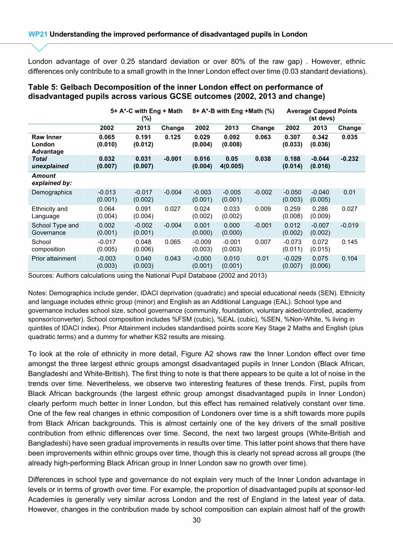
30


London advantage of over 0.25 standard deviation or over 80% of the raw gap) . However, ethnic differences only contribute to a small growth in the Inner London effect over time (0.03 standard deviations).

Table 5: Gelbach Decomposition of the inner London effect on performance of disadvantaged pupils across various GCSE outcomes (2002, 2013 and change)

5+ A*-C with Eng + Math (%)

8+ A*-B with Eng +Math (%) Average Capped Points (st devs)


Raw Inner London Advantage

0.065 (0.010)

0.191 (0.012)

0.125 0.029 (0.004)

0.092 (0.008)

0.063 0.307 (0.033)

0.342 (0.036)

0.035

Total unexplained

0.032 (0.007)

0.031 (0.007)

-0.001 0.016 (0.004)

0.05 4(0.005)

0.038 0.188 (0.014)

-0.044 (0.016)

-0.232

Amount explained by: Demographics -0.013

(0.001) -0.017 (0.002)

-0.004 -0.003 (0.001)

-0.005 (0.001)

-0.002 -0.050 (0.003)

-0.040 (0.005)

0.01

Ethnicity and Language

0.064 (0.004)

0.091 (0.004)

0.027 0.024 (0.002)

0.033 (0.002)

0.009 0.259 (0.008)

0.286 (0.009)

0.027

School Type and Governance

0.002 (0.001)

-0.002 (0.001)

-0.004 0.001 (0.000)

0.000 (0.000)

-0.001 0.012 (0.002)

-0.007 (0.002)

-0.019

School composition

-0.017 (0.005)

0.048 (0.006)

0.065 -0.009 (0.003)

-0.001 (0.003)

0.007 -0.073 (0.011)

0.072 (0.015)

0.145

Prior attainment -0.003 (0.003)

0.040 (0.003)

0.043 -0.000 (0.001)

0.010 (0.001)

0.01 -0.029 (0.007)

0.075 (0.006)

0.104

Sources: Authors calculations using the National Pupil Database (2002 and 2013) Notes: Demographics include gender, IDACI deprivation (quadratic) and special educational needs (SEN). Ethnicity and language includes ethnic group (minor) and English as an Additional Language (EAL). School type and governance includes school size, school governance (community, foundation, voluntary aided/controlled, academy sponsor/converter). School composition includes %FSM (cubic), %EAL (cubic), %SEN, %Non-White, % living in quintiles of IDACI index). Prior Attainment includes standardised points score Key Stage 2 Maths and English (plus quadratic terms) and a dummy for whether KS2 results are missing.

To look at the role of ethnicity in more detail, Figure A2 shows raw the Inner London effect over time amongst the three largest ethnic groups amongst disadvantaged pupils in Inner London (Black African, Bangladeshi and White-British). The first thing to note is that there appears to be quite a lot of noise in the trends over time. Nevertheless, we observe two interesting features of these trends. First, pupils from Black African backgrounds (the largest ethnic group amongst disadvantaged pupils in Inner London) clearly perform much better in Inner London, but this effect has remained relatively constant over time. One of the few real changes in ethnic composition of Londoners over time is a shift towards more pupils from Black African backgrounds. This is almost certainly one of the key drivers of the small positive contribution from ethnic differences over time. Second, the next two largest groups (White-British and Bangladeshi) have seen gradual improvements in results over time. This latter point shows that there have been improvements within ethnic groups over time, though this is clearly not spread across all groups (the already high-performing Black African group in Inner London saw no growth over time).

Differences in school type and governance do not explain very much of the Inner London advantage in levels or in terms of growth over time. For example, the proportion of disadvantaged pupils at sponsor-led Academies is generally very similar across London and the rest of England in the latest year of data. However, changes in the contribution made by school composition can explain almost half of the growth

31


in the Inner London effect for the standard benchmark (5 or more GCSEs at A*-C including English and Maths) and around one sixth of the growth in the Inner London effect on the measure of higher performance (8 or more A*-B including English and Maths). For the average points score, the contribution made by school composition shifts from a negative contribution of just over 0.07 standard deviations to a positive contribution of 0.07.

The large and changing contribution made by school composition in explaining the increasing Inner London effect warrants further discussion. First, Appendix Table A3 performs an even more detailed version of the decomposition, which shows that the increasing contribution from school composition comes largely from socio-economic composition of pupils. Second, it is important to check whether the changing contribution comes from a change in levels or coefficients. We already know from the previous section that the average levels of the school composition variables were not changing differentially across this period. Figure A2 confirms this and shows that the distributions of the percentage of children eligible for FSM across schools in Inner London and the rest of England are quite stable over time. This suggests that it is changing coefficients that are driving the changing contribution of school composition variables. Figure A3 confirms this by plotting the relationship between the proportion of children eligible for FSM and the proportion achieving the standard benchmark. This reveals that the relationship between school deprivation and individual results has changed dramatically for Inner London. In 2002, there was a strongly negative relationship between having more deprived peers and one’s own results for both Inner London and the rest of England. This association has become slightly less negative for the rest of England in 2013. However in 2013 there is no longer a negative relationship for children in Inner London. This is a dramatic turnaround. What could be driving this changing relationship?

It is well known that estimating the effect of peers groups on outcomes is fraught with difficulties, such as bias caused by sorting (parents with more able pupils might seek out ‘better’ peer groups) and the reflection problem (an individual can have an effect on one’s peers as well as vice versa), see Manski (1993) for further discussion. As a result, the changing coefficients on the school composition variables could reflect a number of factors. However, it seems unlikely that the reflection bias is changing so dramatically over time and change in the sorting bias is unlikely as we observe little average change in the composition of schools over time.

Usually, the impact of peers is found to be small; except in extreme cases (Lavy et al, 2012). Interestingly, a key defining feature of peer groups in Inner London is that they are extreme, with an average figure of around 43% of children eligible for FSM in schools in Inner London compared with around 20% for the rest of England in 2013. Figure A2 also confirms that there are many schools in Inner London with proportions of children eligible for FSM that are almost nonexistent outside of London (e.g. many schools with levels above 50%). Figure A3 demonstrates that it is at the extreme levels of FSM composition where the changes have been most dramatic. We therefore speculate that the most likely explanation is that school quality has improved in a dimension that has mitigated the impact of having particularly high numbers of peers from deprived backgrounds. However, further research is clearly needed to better understand the changing role of school composition in London over time.

Finally, prior attainment also makes a substantial positive contribution to the growth in the Inner London effect over time. Changes in the role of prior attainment can explain about one third of the growth in the Inner London effect for the standard benchmark and about one sixth of the growth in the Inner London effect for the measure of high performance. For the average point score, we estimate that changes in the

32


role of prior attainment would be sufficient to push up the Inner London effect by over 0.1 standard deviations between 2002 and 2013, other things being equal.

The substantial role played by prior attainment suggests that part of the growth in the Inner London effect on age 16 results can be explained by the fact that children are entering London’s secondary schools with higher levels of ability in Maths and English, suggesting a potentially important role for London’s primary schools. Indeed, section 4 revealed an increase in the raw Inner London effect at age 11. This is then picked up by the prior attainment effect seen in Table 6.

In Appendix Table A5, we decompose the change in prior attainment at age 11, which shows that the vast majority of the growth in English test scores is unexplained by pupil and school characteristics, and about half of the (smaller) growth in Maths scores is also unexplained. This suggests that changes in pupil and school characteristics are unlikely to be the main source of rising prior attainment. However, this analysis is limited by the lack of data on attainment prior to the age 11 (we address this weakness in our analysis of the MCS below).

The second row of Table 7 shows how much of the Inner London effect remains after controlling for the full set of pupil and school characteristics.

For the standard benchmark, there is no longer any growth in the Inner London effect over time. This suggests that the growth in the Inner London effect over time is fully explained by differences and changes in pupil and school characteristics for these outcomes. For the measure of higher performance, there remains growth in the Inner London effect over time. Indeed, over half of the growth remains unexplained. However, for the average points score there is less growth in the Inner London effect over time and a reduction after we control for observable characteristics. This may reflect the lower propensity of schools in London to make use of equivalent or vocational qualifications.

In summary, differences in the ethnic mix of pupils across London and the rest of England forms a substantial explanation for why disadvantaged pupils have a higher level of performance at age 16 in Inner London. However, these ethnic differences explain much less of the growth over time in the Inner London effect (less than one sixth of the improvement in relative performance). The major explanations for why disadvantaged pupils in Inner London have improved relative to their peers over time are a declining negative influence of school composition and rising prior attainment of pupils entering secondary schools (which between them explain over 80% of the growth in performance in our main outcome of interest). There are, however, differences in the precise contributions of different factors across different GCSE outcomes, but these two influences make a substantial positive contribution to the growth in the Inner London effect across all three. For the measure of higher performance, less of the growth is explained by observable school characteristics, and more potentially could be explained by increased secondary school performance.

c) Longitudinal analysis from the MCS

One important limitation of our previous analysis is that we are unable to examine outcomes earlier than age 11 and thus cannot rule out that differences in unobservable factors (such as pupil ability) are driving our results. It could be the case that pupils in London have become increasingly able; and that this is driving the growth in the London Effect at 11. Furthermore, we are unable to examine the role of parental investments; disadvantaged parents might now invest more in their children in London through home

33


learning and enrichment activities. In this section, we make use of the richer data available in the Millennium Cohort Study to investigate both issues.

In Table 6 we show the results of the decomposition for pupils from the MCS for tests at ages 3, 5 and 11. We show results for various outcomes; for verbal reasoning at age 3; for Communication, Language and Literacy and Maths at age 5; and for English and Maths at age 11 (Key Stage 2). Due to lower sample sizes compared with the NPD, we must look at the overall London effect, rather than Inner London. We show two versions of this decomposition. In panel (a), the first version uses variables which are also included in the National Pupil Database, while the second version, panel (b), adds the wider set of parental characteristics and parental investments as measured in the MCS.

First, it is important to note that the overall raw London effects at Key Stage 2 are similar in the MCS as they are the NPD in 2012 (the KS2 decomposition for overall London effect is shown in Appendix Table A7). This is reassuring, confirming that results across the two datasets are similar. The second aspect to note, which we saw above, is that disadvantaged pupils in London are not ahead in raw terms according to any measure at age 5. There is then strong growth in the London effect on all outcomes between when children start school at age 5 up to age 11 test scores. However, the role played by different characteristics differs across the administrative outcomes and the tests carried out for the survey.

The first MCS decomposition (based on similar variable groupings as in the NPD) shows that some of the growth across ages can be explained by ethnicity and language, but most is unexplained by the pupil and school characteristics found in the NPD. The role of ethnicity in explaining the London advantage age 11 is somewhat strongly than in the NPD, and is particularly large for the test of verbal reasoning taken in the MCS at age 11. As anticipated all of the strong negative London effect in the vocabulary tests is due to London’s ethnic make-up, as are the smaller negative London disadvantage in the Foundation Stage Profile at age 5.

When we account for the wider set of parental characteristics and investments contained in the MCS, the results do change slightly, and the unexplained London effect grows for English and Maths. This occurs because some of the additional variables we have added make a negative contribution to the London Effect, leaving more unexplained. In order to avoid picking up behaviour which reacts to children’s experience at school we have included only variables which related to parenting behaviours at ages 3 and 5; although of course these are likely to be correlated with later behaviour. At age 11 it is clear that London’s children are disadvantaged by the fact that measured parental investments are lower for disadvantaged pupils in London. Adding these variables also increases the positive contribution of ethnicity and language at age 11. London’s minorities do well at school despite the poorer investments they receive at home. Interestingly, there is no suggestion that the share of more recent immigrants benefits London’s schools as the variables which capture this also make a negative contribution.

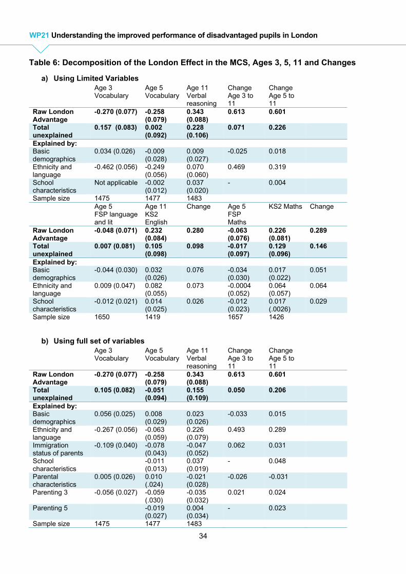
34


Table 6: Decomposition of the London Effect in the MCS, Ages 3, 5, 11 and Changes

a) Using Limited Variables Age 3

Vocabulary Age 5 Vocabulary

Age 11 Verbal reasoning

Change Age 3 to 11

Change Age 5 to 11

Raw London Advantage

-0.270 (0.077) -0.258 (0.079)

0.343 (0.088)

0.613

0.601

Total unexplained

0.157 (0.083) 0.002 (0.092)

0.228 (0.106)

0.071 0.226

Explained by: Basic demographics

0.034 (0.026) -0.009 (0.028)

0.009 (0.027)

-0.025 0.018

Ethnicity and language

-0.462 (0.056) -0.249 (0.056)

0.070 (0.060)

0.469 0.319

School characteristics

Not applicable -0.002 (0.012)

0.037 (0.020)

- 0.004

Sample size 1475 1477 1483 Age 5

FSP language and lit

Age 11 KS2 English

Change Age 5 FSP Maths

KS2 Maths Change


-0.048 (0.071) 0.232 (0.084)

0.280

-0.063 (0.076)

0.226 (0.081)

0.289

Total unexplained

0.007 (0.081) 0.105 (0.098)

0.098 -0.017 (0.097)

0.129 (0.096)

0.146


-0.044 (0.030) 0.032 (0.026)

0.076 -0.034 (0.030)

0.017 (0.022)

0.051


0.009 (0.047) 0.082 (0.055)

0.073 -0.0004 (0.052)

0.064 (0.057)

0.064


-0.012 (0.021) 0.014 (0.025)

0.026 -0.012 (0.023)

0.017 (.0026)

0.029

Sample size 1650 1419 1657 1426

b) Using full set of variables Age 3

Vocabulary Age 5 Vocabulary

Age 11 Verbal reasoning

Change Age 3 to 11

Change Age 5 to 11


-0.270 (0.077) -0.258 (0.079)

0.343 (0.088)

0.613

0.601

Total unexplained

0.105 (0.082) -0.051 (0.094)

0.155 (0.109)

0.050 0.206


0.056 (0.025) 0.008 (0.029)

0.023 (0.026)

-0.033 0.015


-0.267 (0.056) -0.063 (0.059)

0.226 (0.079)

0.493 0.289

Immigration status of parents

-0.109 (0.040) -0.078 (0.043)

-0.047 (0.052)

0.062 0.031


-0.011 (0.013)

0.037 (0.019)

- 0.048

Parental characteristics

0.005 (0.026) 0.010 (.024)

-0.021 (0.028)

-0.026 -0.031

Parenting 3 -0.056 (0.027) -0.059 (.030)

-0.035 (0.032)

0.021 0.024

Parenting 5 -0.019 (0.027)

0.004 (0.034)

- 0.023

Sample size 1475 1477 1483

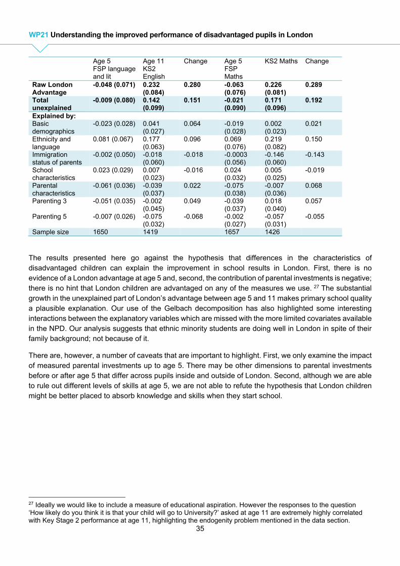
35


Age 5 FSP language and lit

Age 11 KS2 English

Change Age 5 FSP Maths

KS2 Maths Change


-0.048 (0.071) 0.232 (0.084)

0.280

-0.063 (0.076)

0.226 (0.081)

0.289

Total unexplained

-0.009 (0.080) 0.142 (0.099)

0.151 -0.021 (0.090)

0.171 (0.096)

0.192


-0.023 (0.028) 0.041 (0.027)

0.064 -0.019 (0.028)

0.002 (0.023)

0.021


0.081 (0.067) 0.177 (0.063)

0.096

0.069 (0.076)

0.219 (0.082)

0.150

Immigration status of parents

-0.002 (0.050) -0.018 (0.060)

-0.018 -0.0003 (0.056)

-0.146 (0.060)

-0.143


0.023 (0.029) 0.007 (0.023)

-0.016 0.024 (0.032)

0.005 (0.025)

-0.019

Parental characteristics

-0.061 (0.036) -0.039 (0.037)

0.022 -0.075 (0.038)

-0.007 (0.036)

0.068

Parenting 3 -0.051 (0.035) -0.002 (0.045)

0.049 -0.039 (0.037)

0.018 (0.040)

0.057

Parenting 5 -0.007 (0.026) -0.075 (0.032)

-0.068 -0.002 (0.027)

-0.057 (0.031)

-0.055

Sample size 1650 1419 1657 1426

The results presented here go against the hypothesis that differences in the characteristics of disadvantaged children can explain the improvement in school results in London. First, there is no evidence of a London advantage at age 5 and, second, the contribution of parental investments is negative; there is no hint that London children are advantaged on any of the measures we use. 27 The substantial growth in the unexplained part of London’s advantage between age 5 and 11 makes primary school quality a plausible explanation. Our use of the Gelbach decomposition has also highlighted some interesting interactions between the explanatory variables which are missed with the more limited covariates available in the NPD. Our analysis suggests that ethnic minority students are doing well in London in spite of their family background; not because of it.

There are, however, a number of caveats that are important to highlight. First, we only examine the impact of measured parental investments up to age 5. There may be other dimensions to parental investments before or after age 5 that differ across pupils inside and outside of London. Second, although we are able to rule out different levels of skills at age 5, we are not able to refute the hypothesis that London children might be better placed to absorb knowledge and skills when they start school.

27 Ideally we would like to include a measure of educational aspiration. However the responses to the question ‘How likely do you think it is that your child will go to University?’ asked at age 11 are extremely highly correlated with Key Stage 2 performance at age 11, highlighting the endogenity problem mentioned in the data section.

36


6. Conclusion The turnaround in the performance of disadvantaged pupils in London has been a remarkable phenomenon. Having done more poorly at age 16 in the mid-1990s, disadvantaged pupils in Inner London are now 19 percentage points more likely to achieve the standard benchmark of 5 or GCSEs at A*-C (including English and Maths) as compared with disadvantaged pupils outside of London. In this paper we have sought to provide a more detailed understanding of what has driven these improvements. Reflecting on these results, the most important thing to say about the London effect is that the explanation is not simple and does not result from a single policy. The explanation is more complex and stretches back a number of years and through the education system. The basic facts documented here show that the improvement in the performance of disadvantaged pupils in London stretches back to the mid-1990s, is seen across a range of outcomes, is larger for Inner London and is spread across both primary and secondary schools. This already rules out many recent policy initiatives as potential explanations and highlights the possibility that the role of primary schools has been neglected hitherto. Policies such as the London Challenge, Excellence in Cities, the Academies programme and Teach First all began after London’s improvements and were until recently focused only on secondary schools. These policies may have helped build upon London’s success, but are unlikely to have been the primary driving force. One of key differences between London and the rest of England is the higher level of ethnic diversity in London. Difference in the ethnic mix of pupils can explain some of the higher level of performance of disadvantaged pupils in London (consistent with Burgess, 2014). However, they explain much less of the growth in performance of disadvantaged pupils in London. Instead, the growth in the London effect seems more likely to be due to rising school quality across both primary and secondary schools stretching back to the mid-1990s. For primary schools, this is seen in terms of rising age 11 results, largely unexplained by pupil characteristics, which then contributes to better GCSE results. The fact that pupils generally aren’t ahead at age 5, but are by age 11, further suggests that it is contact with schools that is leading to the improved performance. For secondary schools, the improvement in school quality is more nuanced. First, we see much higher levels of performance across measures of high academic performance (i.e. getting 8 or more A*-Bs), unexplained by observable characteristics. Second, there has been a very large decline in the negative contribution made by school composition variables to the London effect. We speculate that this is likely to be due to a declining effect of having very high levels of deprived peers in London; another aspect of the improvement in school quality. The alternative hypothesis is that these changes have been causes by a change in what it means to be deprived in London; in other words London’s deprived children have become less disadvantaged so their performance has improved. Although it is impossible to rule this out we think this is unlikely for a number of reasons. First, we have shown little evidence of changes in the size of the FSM group in London. Second, descriptive statistics on London’s population show that the material conditions of those on benefits have not changed. Third, our MCS analysis shows that for a recent cohort there is no evidence that disadvantaged children are higher ability before they start school or that their parents’ education or occupations are different to those of disadvantaged children outside of London. Finally, our use of the Gelbach decomposition reveals some interesting interactions between parental investments and family background; ethnic minority students are doing well in London in spite of lower measured parental

37


investments, rather than because of them. However, it is important to acknowledge that we are not able to examine all dimensions of parental investments and London’s pupils could differ in terms of their educational trajectories, e.g. their ability to absorb skills. Understanding potential differences in educational trajectories and differences in other parental investments are important topics for future research. It is beyond the scope of this paper to ascribe the improvements in school quality to individual policies, a topic we leave to future research. Indeed, it seems likely that there is not a single explanation. Many aspects of the schooling environment were changing in the mid-1990s in England, with school inspections, choice and competition all recent innovations at that point, as well as specific interventions such as the Literacy Hour. The abolition of the Inner London Education Authority in 1990 may also have accelerated London’s progress as control of education was transferred to London Boroughs. The explanation for London’s success could come from a combination of these policies. London’s schooling success seems likely to further grow over time as age 11 test scores continue to improve relative to elsewhere in England. Furthermore, it is striking that London’s improvement appears to be driven by higher quality attainment, including higher grades and GCSE qualifications rather than lower-value equivalent qualifications. This has important implications for future trends in higher education participation, labour market outcomes and social mobility in London relative to elsewhere. Greaves et al (2014) show that disadvantaged pupils in London are significantly more likely to continue on in post-compulsory education and this has improved over time. This is the first sign that the high quality attainment at 16 is translating into better quality outcomes later in life. While it is too early to observe if this trend continues at later stages, there are reasons to be optimistic that this may translate into more social mobility in the capital city.

38


References

Allen, R., & Allnutt, J. (2013). Matched panel data estimates of the impact of Teach First on school and departmental performance. Institute of Education, DoQSS WP 13.

Almond, D. and Currie J. (2011) “Human Capital Development Before Age Five.” Handbook of Labor Economics, Volume 4, Part B, pp. 1315-1486.

Angrist, J. D., S. M. Dynarski, T. J. Kane, P. A Pathak, and C. R. Walters. (2012). Who Benefits from KIPP? Journal of Policy Analysis and Management. 31(4): 837-860. Belfield, C., Chandler, D. and Joyce, R. (2015), “Housing: trends in prices, costs and tenure,” 2015

Election Briefing Note No 4, Institute for Fiscal Studies Blanden, J. (2013) ‘Cross-national rankings of intergenerational mobility: a comparison of approaches

from economics and sociology’ Journal of Economic Surveys, 27, 38-74. Blanden. J and L. Macmillan (2014) ‘Education and Intergenerational Mobility: Help or Hindrance’ Social

Policy in a Cold Climate Working Paper 08’ CASE, LSE. Blanden, J., P. Gregg and L. Macmillan (2007) ‘Accounting for Intergenerational Persistence:

Noncognitive Skills, Ability and Education’ Economic Journal Conference Volume, C43-C60. Burgess, S. (2014) ‘Understanding the Success of London’s Schools’ CMPO Working Paper No.14/333.

Bristol. Cascio, E and Staiger, D. ‘Knowledge, tests and fadeout in educational inventions’ NBER Working Paper

No. 18038. Carneiro, P. and Heckman, J. (2003), ‘Human Capital Policy, in ‘Inequality in America: What Role for

Human Capital Policies’ (edited by James Heckman and Alan Krueger), MIT Press, 2003. CfBT (2014) Lessons from London Schools: Investigating the Success. CfBT.

http://cdn.cfbt.com/~/media/cfbtcorporate/files/research/2014/r-london-schools-2014.pdf City of London Corporation, (2011), London’s Competitive Place in the UK and Global Economies Cook, C. (2013) ‘London School children perform the best’. Financial Times, 13/1/13 Corak, M. (2013) ‘Income Inequality, Equality of Opportunity, and Intergenerational Mobility Inequality

Journal of Economic Perspectives Volume 27, Number 3—Summer 2013—Pages 79–102. Dearden, L., Sibieta, L. and Sylva, K. (2011) “The socio-economic gradient in early child outcomes:

evidence from the Millennium Cohort Study, “ Longitudinal and Life Course Studies., 2, 19–40. D’Costa and Overman, (2014) ‘The urban wage growth premium. Sorting or learning?’ Regional Science

and Urban Economics, 48, pp. 168-179. Department for Work and Pensions (2015), Household Below Average Income: 1994/95 to 2013/14,

https://www.gov.uk/government/statistics/households-below-average-income-19941995-to-20132014

Duncan, and Murnane (2011) Whither Opportunity? Rising Inequality, Schools and Children’s Life Chances Russell Sage Foundation.

Dustmann, C., S. Machin and U. Schonberg (2010) ‘Ethnicity and Educational Achievement in Compulsory Schooling’ Economic Journal, 120 F272-297.

Freedman, S. (2014) ‘The London Schools Effect – What have we learned this week?’ http://samfreedman1.blogspot.co.uk/2014/06/the-london-schools-effect-what-have-we_28.html

Gelbach (2014) ‘When do covariates matter? And which ones, and how much?’ Journal of Labor Economics, forthcoming.

Goodman, A. and Gregg, P. (2010) (eds) Poorer children’s educational attainment: how important are attitudes and behaviour, Joseph Rowntree Foundation.

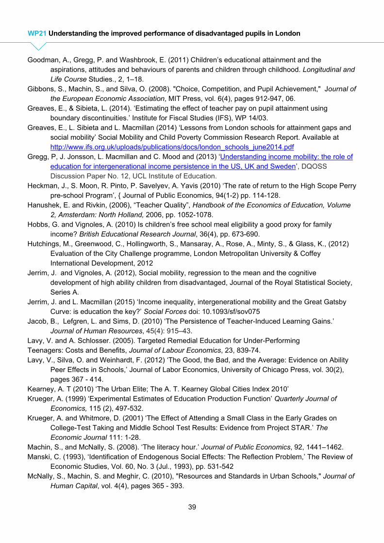
39


Goodman, A., Gregg, P. and Washbrook, E. (2011) Children’s educational attainment and the aspirations, attitudes and behaviours of parents and children through childhood. Longitudinal and Life Course Studies., 2, 1–18.

Gibbons, S., Machin, S., and Silva, O. (2008). "Choice, Competition, and Pupil Achievement," Journal of the European Economic Association, MIT Press, vol. 6(4), pages 912-947, 06.

Greaves, E., & Sibieta, L. (2014). ‘Estimating the effect of teacher pay on pupil attainment using boundary discontinuities.’ Institute for Fiscal Studies (IFS), WP 14/03.

Greaves, E., L. Sibieta and L. Macmillan (2014) ‘Lessons from London schools for attainment gaps and social mobility’ Social Mobility and Child Poverty Commission Research Report. Available at http://www.ifs.org.uk/uploads/publications/docs/london_schools_june2014.pdf

Gregg, P, J. Jonsson, L. Macmillan and C. Mood and (2013) ‘Understanding income mobility: the role of education for intergenerational income persistence in the US, UK and Sweden’, DQOSS Discussion Paper No. 12, UCL Institute of Education.

Heckman, J., S. Moon, R. Pinto, P. Savelyev, A. Yavis (2010) ‘The rate of return to the High Scope Perry pre-school Program’, { Journal of Public Economics, 94(1-2) pp. 114-128.

Hanushek, E. and Rivkin, (2006), “Teacher Quality”, Handbook of the Economics of Education, Volume 2, Amsterdam: North Holland, 2006, pp. 1052-1078.

Hobbs, G. and Vignoles, A. (2010) Is children’s free school meal eligibility a good proxy for family income? British Educational Research Journal, 36(4), pp. 673-690.

Hutchings, M., Greenwood, C., Hollingworth, S., Mansaray, A., Rose, A., Minty, S., & Glass, K., (2012) Evaluation of the City Challenge programme, London Metropolitan University & Coffey International Development, 2012

Jerrim, J. and Vignoles, A. (2012), Social mobility, regression to the mean and the cognitive development of high ability children from disadvantaged, Journal of the Royal Statistical Society, Series A.

Jerrim, J. and L. Macmillan (2015) ‘Income inequality, intergenerational mobility and the Great Gatsby Curve: is education the key?’ Social Forces doi: 10.1093/sf/sov075

Jacob, B., Lefgren, L. and Sims, D. (2010) ‘The Persistence of Teacher-Induced Learning Gains.’ Journal of Human Resources, 45(4): 915–43.

Lavy, V. and A. Schlosser. (2005). Targeted Remedial Education for Under-Performing Teenagers: Costs and Benefits, Journal of Labour Economics, 23, 839-74. Lavy, V., Silva, O. and Weinhardt, F. (2012) ‘The Good, the Bad, and the Average: Evidence on Ability

Peer Effects in Schools,’ Journal of Labor Economics, University of Chicago Press, vol. 30(2), pages 367 - 414.

Kearney, A. T (2010) ‘The Urban Elite; The A. T. Kearney Global Cities Index 2010’ Krueger, A. (1999) ‘Experimental Estimates of Education Production Function’ Quarterly Journal of

Economics, 115 (2), 497-532. Krueger, A. and Whitmore, D. (2001) ‘The Effect of Attending a Small Class in the Early Grades on

College-Test Taking and Middle School Test Results: Evidence from Project STAR.’ The Economic Journal 111: 1-28.

Machin, S., and McNally, S. (2008). ‘The literacy hour.’ Journal of Public Economics, 92, 1441–1462. Manski, C. (1993), ‘Identification of Endogenous Social Effects: The Reflection Problem,’ The Review of

Economic Studies, Vol. 60, No. 3 (Jul., 1993), pp. 531-542 McNally, S., Machin, S. and Meghir, C. (2010), "Resources and Standards in Urban Schools," Journal of

Human Capital, vol. 4(4), pages 365 - 393.

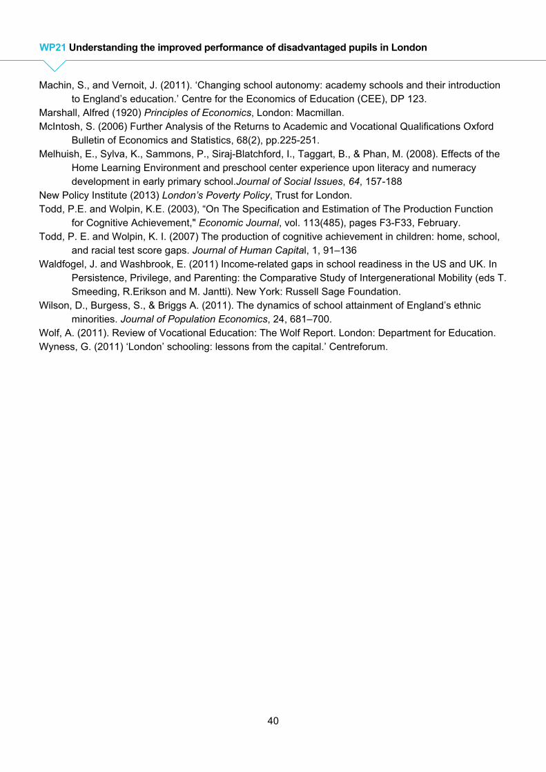
40


Machin, S., and Vernoit, J. (2011). ‘Changing school autonomy: academy schools and their introduction to England’s education.’ Centre for the Economics of Education (CEE), DP 123.

Marshall, Alfred (1920) Principles of Economics, London: Macmillan. McIntosh, S. (2006) Further Analysis of the Returns to Academic and Vocational Qualifications Oxford

Bulletin of Economics and Statistics, 68(2), pp.225-251. Melhuish, E., Sylva, K., Sammons, P., Siraj-Blatchford, I., Taggart, B., & Phan, M. (2008). Effects of the

Home Learning Environment and preschool center experience upon literacy and numeracy development in early primary school.Journal of Social Issues, 64, 157-188

New Policy Institute (2013) London’s Poverty Policy, Trust for London. Todd, P.E. and Wolpin, K.E. (2003), “On The Specification and Estimation of The Production Function

for Cognitive Achievement," Economic Journal, vol. 113(485), pages F3-F33, February. Todd, P. E. and Wolpin, K. I. (2007) The production of cognitive achievement in children: home, school,

and racial test score gaps. Journal of Human Capital, 1, 91–136 Waldfogel, J. and Washbrook, E. (2011) Income-related gaps in school readiness in the US and UK. In

Persistence, Privilege, and Parenting: the Comparative Study of Intergenerational Mobility (eds T. Smeeding, R.Erikson and M. Jantti). New York: Russell Sage Foundation.

Wilson, D., Burgess, S., & Briggs A. (2011). The dynamics of school attainment of England’s ethnic minorities. Journal of Population Economics, 24, 681–700.

Wolf, A. (2011). Review of Vocational Education: The Wolf Report. London: Department for Education. Wyness, G. (2011) ‘London’ schooling: lessons from the capital.’ Centreforum.

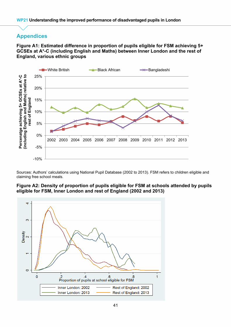
41


Appendices

Figure A1: Estimated difference in proportion of pupils eligible for FSM achieving 5+ GCSEs at A*-C (including English and Maths) between Inner London and the rest of England, various ethnic groups

Sources: Authors’ calculations using National Pupil Database (2002 to 2013). FSM refers to children eligible and claiming free school meals.

Figure A2: Density of proportion of pupils eligible for FSM at schools attended by pupils eligible for FSM, Inner London and rest of England (2002 and 2013)

-10%

-5%

0%

5%

10%

15%

20%

25%

2002 2003 2004 2005 2006 2007 2008 2009 2010 2011 2012 2013

Per

cen

atg

e ac

hie

vin

g 5

+ G

CS

Es

at A

*-C

(i

ncl

ud

ing

En

glis

h a

nd

Mat

hs)

rel

ativ

e to

re

st o

f E

ng

lan

d

White British Black African Bangladeshi

42


Figure A3: Local linear regression estimates of relationship between proportion of pupils eligible at a school and GCSE performance amongst pupils eligible for FSM, Inner London and rest of England (2002 and 2013)

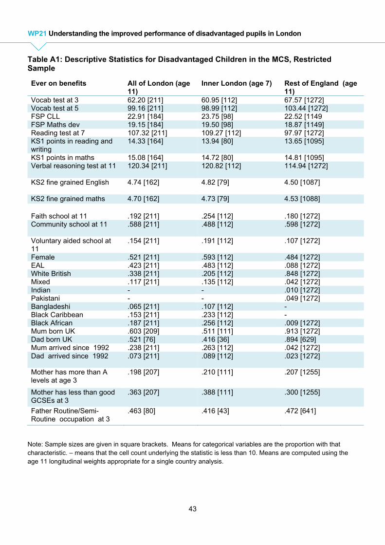
43


Table A1: Descriptive Statistics for Disadvantaged Children in the MCS, Restricted Sample

Ever on benefits All of London (age 11)

Inner London (age 7) Rest of England (age 11)

Vocab test at 3 62.20 [211] 60.95 [112] 67.57 [1272] Vocab test at 5 99.16 [211] 98.99 [112] 103.44 [1272] FSP CLL 22.91 [184] 23.75 [98] 22.52 [1149 FSP Maths dev 19.15 [184] 19.50 [98] 18.87 [1149] Reading test at 7 107.32 [211] 109.27 [112] 97.97 [1272] KS1 points in reading and writing

14.33 [164] 13.94 [80] 13.65 [1095]

KS1 points in maths 15.08 [164] 14.72 [80] 14.81 [1095] Verbal reasoning test at 11 120.34 [211] 120.82 [112] 114.94 [1272]

KS2 fine grained English 4.74 [162] 4.82 [79] 4.50 [1087]

KS2 fine grained maths 4.70 [162] 4.73 [79] 4.53 [1088] Faith school at 11 .192 [211] .254 [112] .180 [1272] Community school at 11 .588 [211] .488 [112] .598 [1272]

Voluntary aided school at 11

.154 [211] .191 [112] .107 [1272]

Female .521 [211] .593 [112] .484 [1272] EAL .423 [211] .483 [112] .088 [1272] White British .338 [211] .205 [112] .848 [1272] Mixed .117 [211] .135 [112] .042 [1272] Indian - - .010 [1272] Pakistani - - .049 [1272] Bangladeshi .065 [211] .107 [112] - Black Caribbean .153 [211] .233 [112] - Black African .187 [211] .256 [112] .009 [1272] Mum born UK .603 [209] .511 [111] .913 [1272] Dad born UK .521 [76] .416 [36] .894 [629] Mum arrived since 1992 .238 [211] .263 [112] .042 [1272] Dad arrived since 1992 .073 [211] .089 [112] .023 [1272]

Mother has more than A levels at age 3

.198 [207] .210 [111] .207 [1255]

Mother has less than good GCSEs at 3

.363 [207] .388 [111] .300 [1255]

Father Routine/Semi-Routine occupation at 3

.463 [80] .416 [43] .472 [641]

Note: Sample sizes are given in square brackets. Means for categorical variables are the proportion with that characteristic. – means that the cell count underlying the statistic is less than 10. Means are computed using the age 11 longitudinal weights appropriate for a single country analysis.

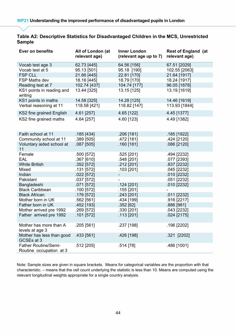
44


Table A2: Descriptive Statistics for Disadvantaged Children in the MCS, Unrestricted Sample

Ever on benefits All of London (at relevant age)

Inner London (relevant age up to 7)

Rest of England (at relevant age)

Vocab test age 3 62.73 [445] 64.56 [156] 67.51 [2029] Vocab test at 5 95.13 [501] 95.18 [190] 102.55 [2063] FSP CLL 21.66 [445] 22.81 [170] 21.64 [1917] FSP Maths dev 18.16 [445] 18.79 [170] 18.24 [1917] Reading test at 7 102.74 [437] 104.74 [177] 96.05 [1878] KS1 points in reading and writing

13.44 [325] 13.15 [125] 13.19 [1619]

KS1 points in maths 14.58 [325] 14.28 [125] 14.46 [1619] Verbal reasoning at 11 118.58 [421] 118.82 [147] 113.93 [1844]

KS2 fine grained English 4.61 [257] 4.65 [122] 4.45 [1377]

KS2 fine grained maths 4.64 [257] 4.60 [123] 4.49 [1382]

Faith school at 11 .185 [434] .206 [181] .185 [1922] Community school at 11 .389 [505] .472 [181] .424 [2120] Voluntary aided school at 11

.087 [505] .160 [181] .086 [2120]

Female .500 [572] .525 [201] .494 [2232] EAL .367 [610] .548 [201] .077 [2393] White British .352 [572] .212 [201] .837 [2232] Mixed .131 [572] .103 [201] .045 [2232] Indian .022 [572] - .010 [2232] Pakistani .037 [572] - .051 [2232] Bangladeshi .071 [572] .124 [201] .010 [2232] Black Caribbean .100 [572] .155 [201] - Black African .176 [572] .243 [201] .011 [2232] Mother born in UK .562 [561] .434 [199] .916 [2217] Father born in UK .452 [193] .352 [62] .886 [981] Mother arrived pre 1992 .269 [572] .330 [201] .043 [2232] Father arrived pre 1992 .101 [572] .113 [201] .024 [2175]

Mother has more than A levels at age 3

.205 [561] .237 [198] .196 [2202]

Mother has less than good GCSEs at 3

.433 [561] .426 [198] .321 [2202]

Father Routine/Semi-Routine occupation at 3

.512 [205] .514 [78] .486 [1001]

Note: Sample sizes are given in square brackets. Means for categorical variables are the proportion with that characteristic. – means that the cell count underlying the statistic is less than 10. Means are computed using the relevant longitudinal weights appropriate for a single country analysis.

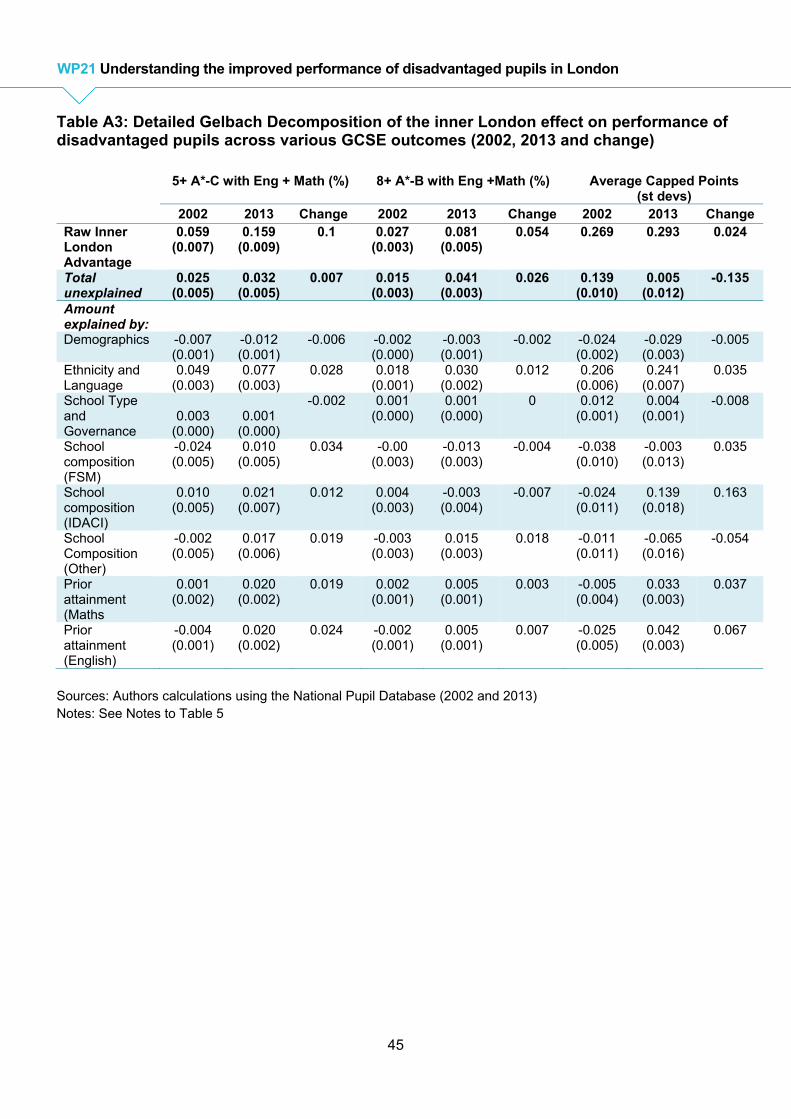
45


Table A3: Detailed Gelbach Decomposition of the inner London effect on performance of disadvantaged pupils across various GCSE outcomes (2002, 2013 and change)

Sources: Authors calculations using the National Pupil Database (2002 and 2013) Notes: See Notes to Table 5

5+ A*-C with Eng + Math (%) 8+ A*-B with Eng +Math (%) Average Capped Points (st devs)

2002 2013 Change 2002 2013 Change 2002 2013 Change Raw Inner London Advantage

0.059 (0.007)

0.159 (0.009)

0.1 0.027 (0.003)

0.081 (0.005)

0.054 0.269 0.293 0.024

Total unexplained

0.025 (0.005)

0.032 (0.005)

0.007 0.015 (0.003)

0.041 (0.003)

0.026 0.139 (0.010)

0.005 (0.012)

-0.135


(0.001) -0.012 (0.001)

-0.006 -0.002 (0.000)

-0.003 (0.001)

-0.002 -0.024 (0.002)

-0.029 (0.003)

-0.005


0.049 (0.003)

0.077 (0.003)

0.028 0.018 (0.001)

0.030 (0.002)

0.012 0.206 (0.006)

0.241 (0.007)

0.035


0.003 (0.000)

0.001 (0.000)

-0.002 0.001 (0.000)

0.001 (0.000)

0 0.012 (0.001)

0.004 (0.001)

-0.008

School composition (FSM)

-0.024 (0.005)

0.010 (0.005)

0.034 -0.00 (0.003)

-0.013 (0.003)

-0.004 -0.038 (0.010)

-0.003 (0.013)

0.035

School composition (IDACI)

0.010 (0.005)

0.021 (0.007)

0.012 0.004 (0.003)

-0.003 (0.004)

-0.007 -0.024 (0.011)

0.139 (0.018)

0.163

School Composition (Other)

-0.002 (0.005)

0.017 (0.006)

0.019 -0.003 (0.003)

0.015 (0.003)

0.018 -0.011 (0.011)

-0.065 (0.016)

-0.054

Prior attainment (Maths

0.001 (0.002)

0.020 (0.002)

0.019 0.002 (0.001)

0.005 (0.001)

0.003 -0.005 (0.004)

0.033 (0.003)

0.037

Prior attainment (English)

-0.004 (0.001)

0.020 (0.002)

0.024 -0.002 (0.001)

0.005 (0.001)

0.007 -0.025 (0.005)

0.042 (0.003)

0.067

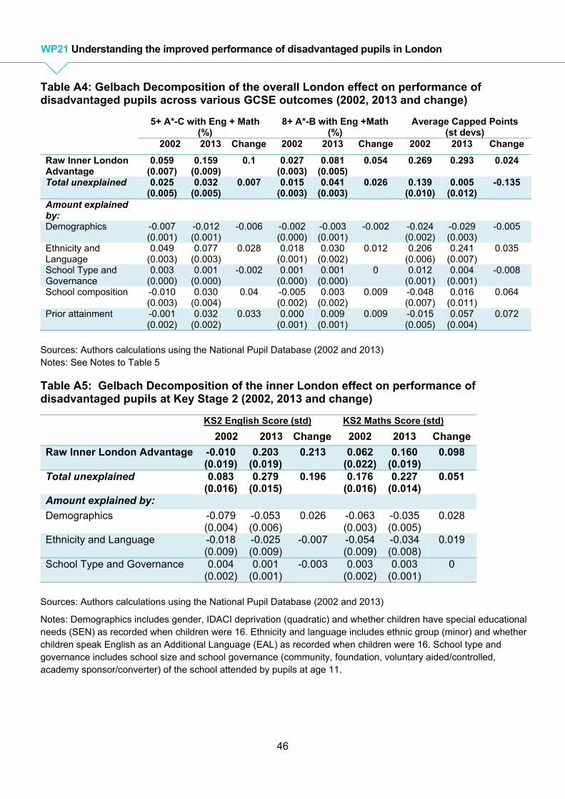
46


Table A4: Gelbach Decomposition of the overall London effect on performance of disadvantaged pupils across various GCSE outcomes (2002, 2013 and change)

5+ A*-C with Eng + Math (%)

8+ A*-B with Eng +Math (%)

Average Capped Points (st devs)



0.059 (0.007)

0.159 (0.009)

0.1 0.027 (0.003)

0.081 (0.005)

0.054 0.269 0.293 0.024

Total unexplained 0.025 (0.005)

0.032 (0.005)

0.007 0.015 (0.003)

0.041 (0.003)

0.026 0.139 (0.010)

0.005 (0.012)

-0.135


(0.001) -0.012 (0.001)

-0.006 -0.002 (0.000)

-0.003 (0.001)

-0.002 -0.024 (0.002)

-0.029 (0.003)

-0.005


0.049 (0.003)

0.077 (0.003)

0.028 0.018 (0.001)

0.030 (0.002)

0.012 0.206 (0.006)

0.241 (0.007)

0.035


0.003 (0.000)

0.001 (0.000)

-0.002 0.001 (0.000)

0.001 (0.000)

0 0.012 (0.001)

0.004 (0.001)

-0.008

School composition -0.010 (0.003)

0.030 (0.004)

0.04 -0.005 (0.002)

0.003 (0.002)

0.009 -0.048 (0.007)

0.016 (0.011)

0.064

Prior attainment -0.001 (0.002)

0.032 (0.002)

0.033 0.000 (0.001)

0.009 (0.001)

0.009 -0.015 (0.005)

0.057 (0.004)

0.072


Table A5: Gelbach Decomposition of the inner London effect on performance of disadvantaged pupils at Key Stage 2 (2002, 2013 and change)

KS2 English Score (std) KS2 Maths Score (std)

2002 2013 Change 2002 2013 Change

Raw Inner London Advantage -0.010 (0.019)

0.203 (0.019)

0.213 0.062 (0.022)

0.160 (0.019)

0.098


0.279 (0.015)

0.196 0.176 (0.016)

0.227 (0.014)

0.051

Amount explained by:

Demographics -0.079 (0.004)

-0.053 (0.006)

0.026 -0.063 (0.003)

-0.035 (0.005)

0.028

Ethnicity and Language -0.018 (0.009)

-0.025 (0.009)

-0.007 -0.054 (0.009)

-0.034 (0.008)

0.019

School Type and Governance 0.004 (0.002)

0.001 (0.001)

-0.003 0.003 (0.002)

0.003 (0.001)

0

Sources: Authors calculations using the National Pupil Database (2002 and 2013)

Notes: Demographics includes gender, IDACI deprivation (quadratic) and whether children have special educational needs (SEN) as recorded when children were 16. Ethnicity and language includes ethnic group (minor) and whether children speak English as an Additional Language (EAL) as recorded when children were 16. School type and governance includes school size and school governance (community, foundation, voluntary aided/controlled, academy sponsor/converter) of the school attended by pupils at age 11.

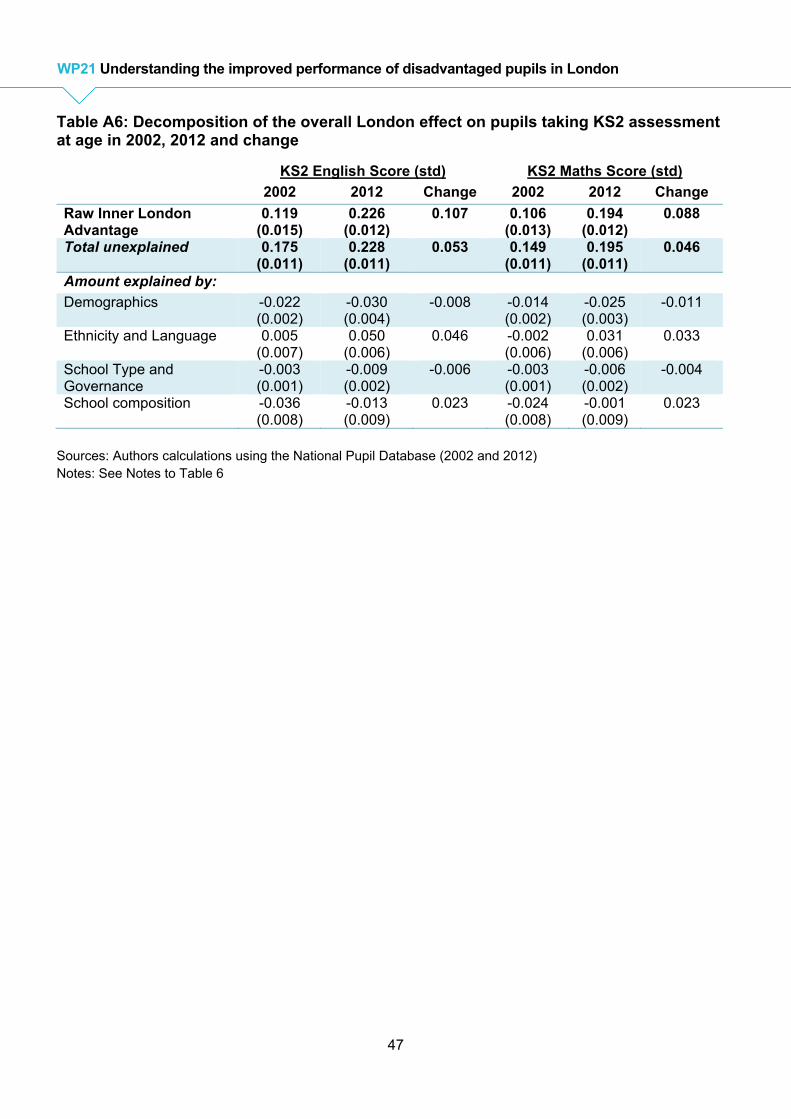
47


Table A6: Decomposition of the overall London effect on pupils taking KS2 assessment at age in 2002, 2012 and change

KS2 English Score (std) KS2 Maths Score (std)

2002 2012 Change 2002 2012 Change


0.119 (0.015)

0.226 (0.012)

0.107 0.106 (0.013)

0.194 (0.012)

0.088


0.228 (0.011)

0.053 0.149 (0.011)

0.195 (0.011)

0.046

Amount explained by:

Demographics -0.022 (0.002)

-0.030 (0.004)

-0.008 -0.014 (0.002)

-0.025 (0.003)

-0.011

Ethnicity and Language 0.005 (0.007)

0.050 (0.006)

0.046 -0.002 (0.006)

0.031 (0.006)

0.033


-0.003 (0.001)

-0.009 (0.002)

-0.006 -0.003 (0.001)

-0.006 (0.002)

-0.004

School composition -0.036 (0.008)

-0.013 (0.009)

0.023 -0.024 (0.008)

-0.001 (0.009)

0.023


understanding the improved performance of disadvantaged...

Documents