understanding hard interaction in qcd and the search for
TRANSCRIPT

University of Massachusetts Amherst University of Massachusetts Amherst
ScholarWorks@UMass Amherst ScholarWorks@UMass Amherst
Open Access Dissertations
5-2012
Understanding Hard Interaction in QCD and the Search for the Understanding Hard Interaction in QCD and the Search for the
Gluon Spin Contribution to the Spin of the Proton Gluon Spin Contribution to the Spin of the Proton
Amaresh Datta University of Massachusetts Amherst
Follow this and additional works at: https://scholarworks.umass.edu/open_access_dissertations
Part of the Physics Commons
Recommended Citation Recommended Citation Datta, Amaresh, "Understanding Hard Interaction in QCD and the Search for the Gluon Spin Contribution to the Spin of the Proton" (2012). Open Access Dissertations. 544. https://doi.org/10.7275/nmcf-qp76 https://scholarworks.umass.edu/open_access_dissertations/544
This Open Access Dissertation is brought to you for free and open access by ScholarWorks@UMass Amherst. It has been accepted for inclusion in Open Access Dissertations by an authorized administrator of ScholarWorks@UMass Amherst. For more information, please contact [email protected].

UNDERSTANDING HARD INTERACTION IN QCD ANDTHE SEARCH FOR THE GLUON SPIN CONTRIBUTION
TO THE SPIN OF THE PROTON
A Dissertation Presented
by
AMARESH DATTA
Submitted to the Graduate School of theUniversity of Massachusetts Amherst in partial fulfillment
of the requirements for the degree of
DOCTOR OF PHILOSOPHY
May, 2012
Physics

c© Copyright by Amaresh Datta 2012
All Rights Reserved

UNDERSTANDING HARD INTERACTION IN QCD ANDTHE SEARCH FOR THE GLUON SPIN CONTRIBUTION
TO THE SPIN OF THE PROTON
A Dissertation Presented
by
AMARESH DATTA
Approved as to style and content by:
David Kawall, Chair
John Donoghue, Member
Krishna Kumar, Member
Grant Wilson, Member
Donald Candela, Department ChairPhysics

To my grandfather, Late Anantalal Datta, the poor refugee from abroken country, who taught the value of education to his children.

ACKNOWLEDGMENTS
I would like to acknowledge here my advisor David Kawall for all the help and
the support from him during the years I worked with him. His unwavering encour-
agements has been a beacon throughout the good and the bad times. Thank you
Dave.
My very special thanks to Christine Aidala for the enormous amount of time and
effort she spent discussing physics (and other things) with me and for her guiding
hand that helped me finish the analyses through a lot of complications. Thank you
Christine.
Jane Knapp, the angel of a graduate secretary in the Physics Department at
UMass, Amherst, deserves the gratitude of generations of graduate students for the
loving smile and the care with which she resolves the regular and the more complicated
official issues for us. Thank you Jane.
v
ABSTRACT
UNDERSTANDING HARD INTERACTION IN QCD ANDTHE SEARCH FOR THE GLUON SPIN CONTRIBUTION
TO THE SPIN OF THE PROTON
MAY, 2012
AMARESH DATTA
B.Sc., JADAVPUR UNIVERSITY
M.Sc., INDIAN INSTITUTE OF TECHNOLOGY, MUMBAI
Ph.D., UNIVERSITY OF MASSACHUSETTS AMHERST
Directed by: Professor David Kawall
In the following discourse unpolarized cross sections and double helicity asymme-
tries of single inclusive positive and negative charged hadrons at mid-rapidity from
p + p collisions at√s = 62.4 GeV are presented. Measurements for the transverse
momentum range 1.0 < pT < 4.5 GeV/c are done with PHENIX detector at Rel-
ativistic Heavy-Ion Collider (RHIC) and are consistent with calculations based on
perturbative quantum chromodynamics (pQCD) at next-to-leading order (NLO) in
the strong coupling constant, αs. Resummed pQCD calculations including terms with
next-to-leading log (NLL) accuracy, yielding reduced theoretical uncertainties, also
agree with the data. The double helicity asymmetry, sensitive at leading order to the
gluon polarization in a momentum fraction range of 0.05 <∼ xgluon<∼ 0.2, is consistent
with recent global parameterizations disfavoring large gluon polarization.
vi

TABLE OF CONTENTS
Page
ACKNOWLEDGMENTS . . . . . . . . . . . . . . . . . . . . . . . . . . . . . . . . . . . . . . . . . . . . . v
ABSTRACT . . . . . . . . . . . . . . . . . . . . . . . . . . . . . . . . . . . . . . . . . . . . . . . . . . . . . . . . . . vi
LIST OF TABLES . . . . . . . . . . . . . . . . . . . . . . . . . . . . . . . . . . . . . . . . . . . . . . . . . . . . x
LIST OF FIGURES . . . . . . . . . . . . . . . . . . . . . . . . . . . . . . . . . . . . . . . . . . . . . . . . . . xii
CHAPTER
1. INTRODUCTION . . . . . . . . . . . . . . . . . . . . . . . . . . . . . . . . . . . . . . . . . . . . . . . . . 1
1.1 Proton Structure . . . . . . . . . . . . . . . . . . . . . . . . . . . . . . . . . . . . . . . . . . . . . . . . . 1
1.1.1 Elastic Structure and Form Factors . . . . . . . . . . . . . . . . . . . . . . . . . . . 11.1.2 Inelastic Structure Functions . . . . . . . . . . . . . . . . . . . . . . . . . . . . . . . . . 51.1.3 Quark Model and QCD . . . . . . . . . . . . . . . . . . . . . . . . . . . . . . . . . . . . . 61.1.4 PDF, Factorization and Universality . . . . . . . . . . . . . . . . . . . . . . . . . . 9
1.2 Spin Structure of Proton . . . . . . . . . . . . . . . . . . . . . . . . . . . . . . . . . . . . . . . . . 111.3 Proton Spin Crisis . . . . . . . . . . . . . . . . . . . . . . . . . . . . . . . . . . . . . . . . . . . . . . . 141.4 Continuing The Search . . . . . . . . . . . . . . . . . . . . . . . . . . . . . . . . . . . . . . . . . . . 15
1.4.1 Polarized DIS and the Evolution Equation . . . . . . . . . . . . . . . . . . . . 151.4.2 Hard Interaction in the Polarized Hadron Collisions . . . . . . . . . . . . 171.4.3 Extracting Gluon Spin Information from Measurements . . . . . . . . 21
1.5 Motivation for Our Measurements . . . . . . . . . . . . . . . . . . . . . . . . . . . . . . . . . 23
2. ACCELERATOR AND DETECTORS . . . . . . . . . . . . . . . . . . . . . . . . . . . . 28
2.1 Polarized Protons at RHIC . . . . . . . . . . . . . . . . . . . . . . . . . . . . . . . . . . . . . . . 28
2.1.1 Polarized Proton Source . . . . . . . . . . . . . . . . . . . . . . . . . . . . . . . . . . . . 292.1.2 Depolarizing Effects and the Siberian Snake . . . . . . . . . . . . . . . . . . 30
vii

2.1.3 Accelerator . . . . . . . . . . . . . . . . . . . . . . . . . . . . . . . . . . . . . . . . . . . . . . . 322.1.4 Polarimeters . . . . . . . . . . . . . . . . . . . . . . . . . . . . . . . . . . . . . . . . . . . . . . 332.1.5 Spin Rotator . . . . . . . . . . . . . . . . . . . . . . . . . . . . . . . . . . . . . . . . . . . . . 35
2.2 PHENIX Detectors . . . . . . . . . . . . . . . . . . . . . . . . . . . . . . . . . . . . . . . . . . . . . . 35
2.2.1 Luminosity Detectors . . . . . . . . . . . . . . . . . . . . . . . . . . . . . . . . . . . . . . 362.2.2 PHENIX Magnets . . . . . . . . . . . . . . . . . . . . . . . . . . . . . . . . . . . . . . . . . 392.2.3 Tracking Detectors . . . . . . . . . . . . . . . . . . . . . . . . . . . . . . . . . . . . . . . . 40
2.2.3.1 Drift Chambers . . . . . . . . . . . . . . . . . . . . . . . . . . . . . . . . . . . 412.2.3.2 Pad Chambers . . . . . . . . . . . . . . . . . . . . . . . . . . . . . . . . . . . . 412.2.3.3 Drift Chamber Quality Analysis . . . . . . . . . . . . . . . . . . . . . 43
2.2.4 Cherenkov Detectors . . . . . . . . . . . . . . . . . . . . . . . . . . . . . . . . . . . . . . . 462.2.5 Particle ID Detectors . . . . . . . . . . . . . . . . . . . . . . . . . . . . . . . . . . . . . . 472.2.6 Electromagnetic Calorimeter . . . . . . . . . . . . . . . . . . . . . . . . . . . . . . . . 482.2.7 Muon Arm Detectors . . . . . . . . . . . . . . . . . . . . . . . . . . . . . . . . . . . . . . 48
3. DATA SELECTION, HADRON TRACK CRITERIA ANDBACKGROUNDS . . . . . . . . . . . . . . . . . . . . . . . . . . . . . . . . . . . . . . . . . . . . . 49
3.1 Data Set . . . . . . . . . . . . . . . . . . . . . . . . . . . . . . . . . . . . . . . . . . . . . . . . . . . . . . . 49
3.1.1 Beam-Shift Calibration . . . . . . . . . . . . . . . . . . . . . . . . . . . . . . . . . . . . 503.1.2 Selection Criteria . . . . . . . . . . . . . . . . . . . . . . . . . . . . . . . . . . . . . . . . . . 53
3.2 Backgrounds . . . . . . . . . . . . . . . . . . . . . . . . . . . . . . . . . . . . . . . . . . . . . . . . . . . . 56
3.2.1 Long-lived Particle Decay . . . . . . . . . . . . . . . . . . . . . . . . . . . . . . . . . . 563.2.2 Short-lived Particle Decay . . . . . . . . . . . . . . . . . . . . . . . . . . . . . . . . . . 573.2.3 Treatment of Backgrounds . . . . . . . . . . . . . . . . . . . . . . . . . . . . . . . . . . 57
3.3 Hadron Species Fractions . . . . . . . . . . . . . . . . . . . . . . . . . . . . . . . . . . . . . . . . . 58
4. CROSS SECTION MEASUREMENT . . . . . . . . . . . . . . . . . . . . . . . . . . . . . 62
4.1 Corrections Factors Appropriate for the Detector . . . . . . . . . . . . . . . . . . . . 63
4.1.1 Acceptance of Detectors and Efficiency of Selection Cuts . . . . . . . 63
4.1.1.1 Applying The Correction . . . . . . . . . . . . . . . . . . . . . . . . . . . 67
4.1.2 Momentum Smearing and Correction . . . . . . . . . . . . . . . . . . . . . . . . 684.1.3 Trigger Bias Correction . . . . . . . . . . . . . . . . . . . . . . . . . . . . . . . . . . . . 70
4.2 Luminosity Normalization and Cross Section Measurement . . . . . . . . . . . . 72
viii

4.2.1 Luminosity Normalization and Vernier Scan . . . . . . . . . . . . . . . . . . 724.2.2 Cross Section Results . . . . . . . . . . . . . . . . . . . . . . . . . . . . . . . . . . . . . . 834.2.3 Uncertainties on Cross Sections . . . . . . . . . . . . . . . . . . . . . . . . . . . . . 83
5. DISCUSSION OF CROSS SECTION RESULTS . . . . . . . . . . . . . . . . . . 86
6. DOUBLE HELICITY ASYMMETRY MEASUREMENT . . . . . . . . . 90
6.1 Measurement and Correction . . . . . . . . . . . . . . . . . . . . . . . . . . . . . . . . . . . . . . 90
6.1.1 Double Helicity Asymmetry and Uncertainty . . . . . . . . . . . . . . . . . . 906.1.2 Multiplicity Correction . . . . . . . . . . . . . . . . . . . . . . . . . . . . . . . . . . . . . 936.1.3 Asymmetry Results . . . . . . . . . . . . . . . . . . . . . . . . . . . . . . . . . . . . . . . . 94
6.2 Cross Checks . . . . . . . . . . . . . . . . . . . . . . . . . . . . . . . . . . . . . . . . . . . . . . . . . . . 95
6.2.1 Single Spin Asymmetries . . . . . . . . . . . . . . . . . . . . . . . . . . . . . . . . . . . 956.2.2 Bunch Shuffling . . . . . . . . . . . . . . . . . . . . . . . . . . . . . . . . . . . . . . . . . . . 97
7. DISCUSSION OF ASYMMETRY RESULTS . . . . . . . . . . . . . . . . . . . . 100
8. CONCLUSIONS AND OUTLOOK . . . . . . . . . . . . . . . . . . . . . . . . . . . . . . 104
8.1 Cross Sections and pQCD . . . . . . . . . . . . . . . . . . . . . . . . . . . . . . . . . . . . . . . 1048.2 Longitudinal Spin Program . . . . . . . . . . . . . . . . . . . . . . . . . . . . . . . . . . . . . . 1048.3 Transverse Spin Program . . . . . . . . . . . . . . . . . . . . . . . . . . . . . . . . . . . . . . . . 111
BIBLIOGRAPHY . . . . . . . . . . . . . . . . . . . . . . . . . . . . . . . . . . . . . . . . . . . . . . . . . . 113
ix

LIST OF TABLES
Table Page
2.1 A list of performance of RHIC in polarized p+ p collisions over theyears. . . . . . . . . . . . . . . . . . . . . . . . . . . . . . . . . . . . . . . . . . . . . . . . . . . . . . . . 30
3.1 Background fractions for positive and negative hadrons in different pTbins. . . . . . . . . . . . . . . . . . . . . . . . . . . . . . . . . . . . . . . . . . . . . . . . . . . . . . . . . 59
3.2 Parameters of the fit (AeBpT + C) to the relative fractions of differentspecies in the hadron mixture. See text for details. . . . . . . . . . . . . . . . . 61
4.1 Fit function parameters for the efficiency curves for different hadronspecies. See text in Sect. 4.1.1 for details. . . . . . . . . . . . . . . . . . . . . . . . . 65
4.2 Scale factors applied to Monte Carlo simulation to account for livedetector area in each quadrant of the detector for positive andnegative hadrons. . . . . . . . . . . . . . . . . . . . . . . . . . . . . . . . . . . . . . . . . . . . . . 66
4.3 Parameter values for smearing correction factor. . . . . . . . . . . . . . . . . . . . . . 70
4.4 Systematic uncertainties of cross section measurements from varioussources. . . . . . . . . . . . . . . . . . . . . . . . . . . . . . . . . . . . . . . . . . . . . . . . . . . . . . 84
4.5 The cross sections of mid-rapidity charged hadron production fromp+ p at
√s = 62.4 GeV as a function of pT are tabulated along
with the corresponding statistical (second column) and systematic(third column) uncertainties. Cross sections and errors for positivehadrons with the feed-down correction for protons and antiprotonsapplied (normalization uncertainty of 11.2% not included). . . . . . . . . . 84
4.6 The cross sections of mid-rapidity charged hadron production from(p+ p at
√s = 62.4 GeV as a function of pT are tabulated along
with the corresponding statistical (second column) and systematic(third column) uncertainties. Cross sections and errors fornegative hadrons with the feed-down correction for protons andantiprotons applied (normalization uncertainty of 11.2% notincluded). . . . . . . . . . . . . . . . . . . . . . . . . . . . . . . . . . . . . . . . . . . . . . . . . . . . 85
x

6.1 Enhancement factors from multiplicity correction . . . . . . . . . . . . . . . . . . . . 93
6.2 The double helicity asymmetries and the statistical uncertainties arepresented as a function of pT for positive and negativenon-identified charged hadrons. The fractional contribution to theyields from weak-decay feed-down to protons and antiprotons isshown; no correction to the asymmetries has been made for thesecontributions. . . . . . . . . . . . . . . . . . . . . . . . . . . . . . . . . . . . . . . . . . . . . . . . . 95
6.3 Table for the comparison of statistical uncertainties of double helicityasymmetry measurements and the rms width of the distributionof bunch shuffled fake asymmetries. . . . . . . . . . . . . . . . . . . . . . . . . . . . . . 98
xi

LIST OF FIGURES
Figure Page
1.1 Measurements of the proton magnetic moment µp by the elasticscattering of electron beam from hydrogen gas [83]. . . . . . . . . . . . . . . . . 4
1.2 Diagrammatic view of Deep Inelastic Scattering. . . . . . . . . . . . . . . . . . . . . . . 6
1.3 Structure function F2(x,Q2) as a function of Q2 and over a widerange of values of x from combined H1 and ZEUS data [3]. . . . . . . . . . . 7
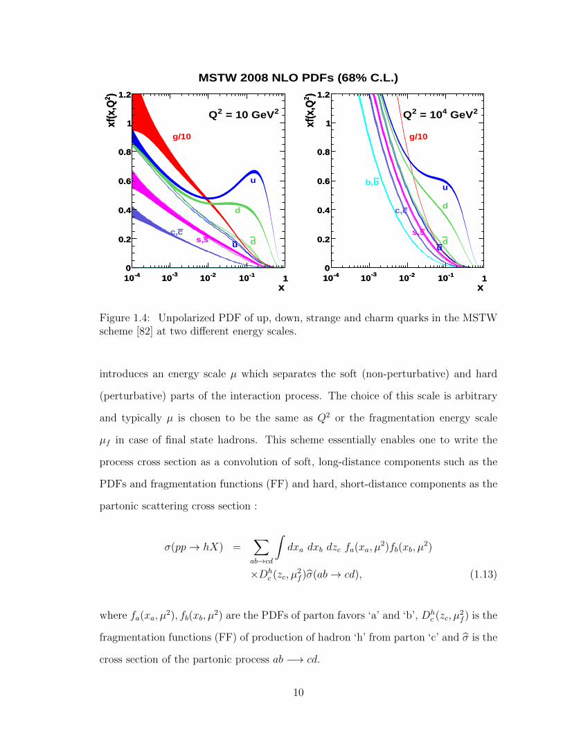
1.4 Unpolarized PDF of up, down, strange and charm quarks in theMSTW scheme [82] at two different energy scales. . . . . . . . . . . . . . . . . . 10
1.5 Polarized PDFs of up and down quarks (LSSparameterizations) [79]. . . . . . . . . . . . . . . . . . . . . . . . . . . . . . . . . . . . . . . . 12
1.6 EMC result in 1989 for∫ 1
0gp1(x)dx contradicting the Ellis-Jaffe Sum
Rule. . . . . . . . . . . . . . . . . . . . . . . . . . . . . . . . . . . . . . . . . . . . . . . . . . . . . . . . 14
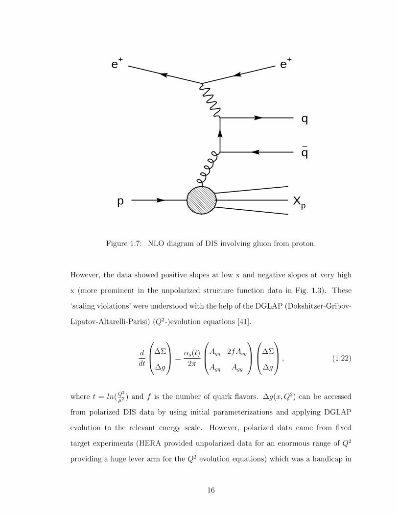
1.7 NLO diagram of DIS involving gluon from proton. . . . . . . . . . . . . . . . . . . . 16
1.8 World data on gp1 from polarized DIS experiments [92]. . . . . . . . . . . . . . . . 17
1.9 Cartoon of a proton-proton collision with a quark-gluon hardscattering producing a pion and other debris X. . . . . . . . . . . . . . . . . . . . 18
1.10 Analyzing power aLL for different partonic subprocesses [50]. . . . . . . . . . . 20
1.11 Sea quark and gluon distributions from DSSV compared to GRSVparameterizations. Shaded bands correspond to ∆χ2 = 1 (onlinecolor green) and ∆χ2/χ2 = 2% (online color yellow) [59]. . . . . . . . . . . . 22
1.12 Partonic sub-process contributions at√s = 62.4 GeV. . . . . . . . . . . . . . . . . 25
1.13 Bjorken x range probed for√s = 62.4 GeV. . . . . . . . . . . . . . . . . . . . . . . . . . 26
1.14 Bjorken x range probed for other RHIC energies. . . . . . . . . . . . . . . . . . . . . 27
xii
2.1 RHIC schematic. . . . . . . . . . . . . . . . . . . . . . . . . . . . . . . . . . . . . . . . . . . . . . . . . 29
2.2 Cartoon showing amplified depolarizing effect with successiverotations of the beam for resonance. . . . . . . . . . . . . . . . . . . . . . . . . . . . . . 32
2.3 Diagram of the magnetic field of a full siberian snake rotating thespin direction by 180. . . . . . . . . . . . . . . . . . . . . . . . . . . . . . . . . . . . . . . . . 32
2.4 Four separate spin patterns of colliding proton bunches used inconsecutive fills at RHIC during 2006. Upper rows show spin ofproton bunches in the ‘blue’ ring at RHIC and the lower rowsshow spin of proton bunches in the ‘yellow’ ring. . . . . . . . . . . . . . . . . . . 33
2.5 PHENIX detector during 2006 data taking period. . . . . . . . . . . . . . . . . . . . 37
2.6 (a) Single Beam Beam Counter consisting of mesh-dynodephoto-multiplier tube on a 3 cm quartz radiator and (b) BBCarray comprising 64 units. [38] . . . . . . . . . . . . . . . . . . . . . . . . . . . . . . . . . . 38
2.7 PHENIX magnets filed lines with (a) Central Magnet in ++configuration and (b) Central Magnet in +− configuration. . . . . . . . . . 40
2.8 Titanium frame defining the DC volume [21]. . . . . . . . . . . . . . . . . . . . . . . . . 42
2.9 Wire configuration in the DC [21]. . . . . . . . . . . . . . . . . . . . . . . . . . . . . . . . . . 43
2.10 The pad and pixel configuration (left). A cell is defined by threepixels (right). [21] . . . . . . . . . . . . . . . . . . . . . . . . . . . . . . . . . . . . . . . . . . . . 44
2.11 Selected tracks as a function of board for the one half of the detectorin the East arm. . . . . . . . . . . . . . . . . . . . . . . . . . . . . . . . . . . . . . . . . . . . . . . 45
2.12 Selected tracks as a function of board for the one half of the detectorin the West arm. . . . . . . . . . . . . . . . . . . . . . . . . . . . . . . . . . . . . . . . . . . . . . 46
2.13 Ratio of normalized (by number of minimum bias events) tracks as afunction of board for the one half of the detector in the Eastarm. . . . . . . . . . . . . . . . . . . . . . . . . . . . . . . . . . . . . . . . . . . . . . . . . . . . . . . . . 46
2.14 Ratio of normalized (by number of minimum bias events) tracks as afunction of board for the one half of the detector in the Westarm. . . . . . . . . . . . . . . . . . . . . . . . . . . . . . . . . . . . . . . . . . . . . . . . . . . . . . . . . 47
3.1 Track reconstruction in the bend (azimuthal) plane at PHENIX. . . . . . . . 51
xiii

3.2 Track reconstruction in the non-bend plane at PHENIX. . . . . . . . . . . . . . . 52
3.3 Sample matching distribution of ‘PC3dφ’ in a pT bin fitted with twoGaussian functions. . . . . . . . . . . . . . . . . . . . . . . . . . . . . . . . . . . . . . . . . . . . 54
3.4 Sample matching distribution of ‘PC3dz’ in a pT bin fitted with twoGaussian functions and a flat component. . . . . . . . . . . . . . . . . . . . . . . . . 55
3.5 Relative fraction of each species for positive hadrons. . . . . . . . . . . . . . . . . . 60
3.6 Relative fraction of each species for negative hadrons. . . . . . . . . . . . . . . . . 61
4.1 Means and widths of Gaussian fits to ‘pc3dφ’ of positive pions asfunction of pT . . . . . . . . . . . . . . . . . . . . . . . . . . . . . . . . . . . . . . . . . . . . . . . . 64
4.2 Means and widths of Gaussian fits to ‘pc3dz’ of positive pions asfunction of pT . . . . . . . . . . . . . . . . . . . . . . . . . . . . . . . . . . . . . . . . . . . . . . . . 65
4.3 Efficiency (includes geometrical acceptance, efficiency of detectorsand efficiency of cuts), for positive hadrons. . . . . . . . . . . . . . . . . . . . . . . 66
4.4 Efficiency (includes geometrical acceptance, efficiency of detectorsand efficiency of cuts), for negative hadrons. . . . . . . . . . . . . . . . . . . . . . . 67
4.5 Combined correction factor for the geometrical acceptance of thedetector and the efficiency of the selection criteria for positivehadrons. . . . . . . . . . . . . . . . . . . . . . . . . . . . . . . . . . . . . . . . . . . . . . . . . . . . . . 68
4.6 Combined correction factor for the geometrical acceptance of thedetector and the efficiency of the selection criteria for negativehadrons. . . . . . . . . . . . . . . . . . . . . . . . . . . . . . . . . . . . . . . . . . . . . . . . . . . . . . 69
4.7 Correction factor for the momentum smearing of reconstructed tracksin the detector. Figure shows fit to the ratio of the positivecharged hadron spectrum in ‘true’ pT vs. that in the ‘smeared’pT . . . . . . . . . . . . . . . . . . . . . . . . . . . . . . . . . . . . . . . . . . . . . . . . . . . . . . . . . . 71
4.8 Parameterized efficiency of Minimum Bias trigger. . . . . . . . . . . . . . . . . . . . 72
4.9 Beam intensity as a function of time during the Vernier scan for fill10478 in 2009 RHIC run. . . . . . . . . . . . . . . . . . . . . . . . . . . . . . . . . . . . . . . 74
4.10 Beam intensity as a function of time during the Vernier scan for fill10505 in 2009 RHIC run. . . . . . . . . . . . . . . . . . . . . . . . . . . . . . . . . . . . . . . 75
xiv

4.11 BBC triggered event rate from global level-1 scalers for fill 10478 in2009 RHIC run. . . . . . . . . . . . . . . . . . . . . . . . . . . . . . . . . . . . . . . . . . . . . . . 76
4.12 BPM position measurements for horizontal Vernier scan of fill 10478in 2009 RHIC run. . . . . . . . . . . . . . . . . . . . . . . . . . . . . . . . . . . . . . . . . . . . . 76
4.13 Calibration of BM steps with steps set by changing magnetic fields forfill 10478 in RHIC 2009 run. Plot a) shows the ratio for horizontalsteps in one side of the beam center and b) shows the ratio for thehorizontal steps in the other side of the beam center. . . . . . . . . . . . . . . 77
4.14 BBC triggered event rate vs. beam position (of a single bunchcrossing) during the horizontal Vernier scan for fill 10478 in 2009RHIC run. . . . . . . . . . . . . . . . . . . . . . . . . . . . . . . . . . . . . . . . . . . . . . . . . . . . 77
4.15 BBC triggered event rate vs. beam position (of a single bunchcrossing) during the vertical Vernier scan for fill 10478 in 2009RHIC run. . . . . . . . . . . . . . . . . . . . . . . . . . . . . . . . . . . . . . . . . . . . . . . . . . . . 78
4.16 Ratio of ‘BBCLL1(> 0 tubes)’ trigger (online cut of 30 cm on vertexposition) to BBC wide trigger (no vertex restriction) for fill 10478in RHIC 2009 run. . . . . . . . . . . . . . . . . . . . . . . . . . . . . . . . . . . . . . . . . . . . . 79
4.17 Ratio of ZDC triggered data with BBC wide trigger and without itfor fill 10478 in RHIC 2009 run. Ratio is fitted to function(Az2 +B). . . . . . . . . . . . . . . . . . . . . . . . . . . . . . . . . . . . . . . . . . . . . . . . . . . . 79
4.18 Figure shows the overlap area of two focused colliding beam for a)head-on collision and b) with a small crossing angle. Cartoon a)demonstrates the appearance of the double-peak structure of thevertex profile as one beam is moved in steps across the other andb) demonstrates the skewness between the two peaks as a result ofthe angle between them. . . . . . . . . . . . . . . . . . . . . . . . . . . . . . . . . . . . . . . . 80
4.19 Vertex profile in beam direction for increasing step sizes (step ∼ 100microns) during the horizontal scan of one of the beams by theother for fill 10478 in RHIC 2009 run. The further the beamcenters are from each other, the more prominent the doublestructure becomes as only the tail regions of the tilted hourglassshape are overlapped. The skewness of the peaks also becomemore appreciable as with increasing steps as overlap on one sidebecomes comparatively larger than that on the other side. . . . . . . . . . . 81
xv
4.20 Comparison of the vertex profile in beam direction for increasing stepsizes for one side of the vertical scans e.g. (1)top-left : step = 0,(2) top-right : step = 200 microns, (3) bottom-left : step = 350microns, (4) bottom-right : step = 500 microns. In thesimulation, β∗ = 70 cm and θ = 0.06 mrad. (Color online) Blackpoints with error bars represent data and open red circlesrepresent simulation. . . . . . . . . . . . . . . . . . . . . . . . . . . . . . . . . . . . . . . . . . . 82
5.1 Cross section of mid-rapidity production of inclusive positive hadronsin p+ p at 62.4 GeV. NLO and NLL theoretical predictions atfactorization, renormalization and fragmentation scale µ = pT areshown on plots. Lower panels show the scale dependence of theNLO and NLL results respectively. . . . . . . . . . . . . . . . . . . . . . . . . . . . . . . 87
5.2 Cross section of mid-rapidity production of inclusive negative hadronsin p+ p at 62.4 GeV. NLO and NLL theoretical predictions atfactorization, renormalization and fragmentation scale µ = pT areshown on plots. Lower panels show the scale dependence of theNLO and NLL results respectively. . . . . . . . . . . . . . . . . . . . . . . . . . . . . . . 88
6.1 Multiplicity distributions of positive hadrons in the transversemomentum bins. . . . . . . . . . . . . . . . . . . . . . . . . . . . . . . . . . . . . . . . . . . . . . 94
6.2 Single spin asymmetries for the ‘blue’ beam for a) positive and b)negative hadrons. . . . . . . . . . . . . . . . . . . . . . . . . . . . . . . . . . . . . . . . . . . . . . 96
6.3 Single spin asymmetries for the ‘yellow’ beam for a) positive and b)negative hadrons. . . . . . . . . . . . . . . . . . . . . . . . . . . . . . . . . . . . . . . . . . . . . . 97
6.4 Distribution of bunch shuffled asymmetries for positive hadrons inthe four pT bins. The rms widths are, respectively, . . . . . . . . . . . . . . . 99
7.1 ALL of mid-rapidity inclusive positive hadron production inproton-proton collisions at
√s = 62.4 GeV with next-to-leading
order calculations. . . . . . . . . . . . . . . . . . . . . . . . . . . . . . . . . . . . . . . . . . . . 101
7.2 ALL of mid-rapidity inclusive negative hadron production inproton-proton collisions at
√s = 62.4 GeV with next-to-leading
order calculations. . . . . . . . . . . . . . . . . . . . . . . . . . . . . . . . . . . . . . . . . . . . 102
8.1 Cross sections of mid-rapidity π0 production in proton-protoncollisions (a) at
√s = 62.4 GeV [15], (b) at
√s = 200 GeV [13]
and (c) at√s = 500 GeV (PHENIX preliminary) are compared to
next-to-leading order pQCD calculations. . . . . . . . . . . . . . . . . . . . . . . . 105
xvi
8.2 Several predictions for ∆G in the pre-RHIC period![1]. . . . . . . . . . . . . . . . 106
8.3 Neutral pion double helicity asymmetry measurements from p+ p at√s = 200 GeV at PHENIX over the years (a) shown separately [1]
and (b) combined (PHENIX preliminary) [1] and compared tocalculated asymmetries using DSSV polarized PDFs. . . . . . . . . . . . . . 107
8.4 Double helicity asymmetry measurements from p+ p at PHENIX for(a) π0 production at
√s = 62.4 GeV [15] and (b) charged pion
production at√s = 200 GeV (PHENIX preliminary) [1]. . . . . . . . . . . 108
8.5 Double helicity asymmetry measurements from p+ p at√s = 200
GeV at PHENIX for (a) η production [17] and (b) direct photonproduction (PHENIX preliminary) [1]. . . . . . . . . . . . . . . . . . . . . . . . . . . 109
8.6 Next-to-leading order estimation of ∆g(x) at Q2 = 4GeV2 in (a)2002 [92] and at Q2 = 10GeV2 in (b) 2008 [59]. . . . . . . . . . . . . . . . . . . 109
8.7 Single helicity asymmetry AL of W boson for two differentcharges [18]. . . . . . . . . . . . . . . . . . . . . . . . . . . . . . . . . . . . . . . . . . . . . . . . . 110
xvii

CHAPTER 1
INTRODUCTION
The proton, which is a universal building block of all atoms, was named after the
Greek word for ‘first’. It was thought to be a fundamental particle in the early parts of
the twentieth century. In 1933, measurements by Esterman, Frisch and Stern [69, 67]
showed that the proton had a large anomalous magnetic moment∼ 2.79 µN , giving the
first indications that protons are not fundamental point-like particles and that they
might be composite particles. Physicists have since worked towards understanding
the structure of the proton and we have come a long way [45] in the decades that
followed. Although our knowledge of the nucleon structure today is considerable,
it is still incomplete, in particular with regard to its spin structure, as we’ll see in
the following sections. With the measurements of cross sections and double helicity
asymmetries of mid-rapidity production of inclusive charged hadrons in p+p collisions
at√s = 62.4 GeV, we aim to get insights into QCD, the fundamental theory of strong
force as a description of hard scattering processes, as well as the spin structure of the
proton.
1.1 Proton Structure
1.1.1 Elastic Structure and Form Factors
Scattering experiments are performed to probe the structure of a particle. The
more energetic the scattered particles are, the smaller is the length scale probed by
them (according to de Broglie, length scale λ ∼ 1/p where p is the momentum).
Scattering of the alpha particles (He nuclei) through thin (thickness ∼ micron) gold
1

foil by Ernest Rutherford in 1911 proved the substructure of atoms and the presence of
the much smaller nuclei inside atoms. A few years later passage of the energetic alpha
particles through hydrogen gas produced hydrogen nuclei and with the considerations
of atomic weights, it was conjectured to be a common building block for all atoms
(nuclei). Rutherford named it as the ‘proton’.
Electrons (and muons) have been used over the decades for probing the structure
of the proton through scattering experiments. In the non-relativistic limit, neglecting
the proton recoil and summing over all possible helicity states of the scattered elec-
trons, the results from the scattering experiments can be described by the Rutherford
scattering cross section :
(dσ
dΩ
)Rutherford
=α2m2
e
4p4 sin4 θ2
, (1.1)
where α is the fine structure constant, p is the momentum of the electron, me is the
electron mass and θ is the scattering angle. It can be concluded that when the length
scales probed are much larger than the proton charge radius, the protons behave
as charged point particles. Considering relativistic scattered particles (p me and
conserving the helicity state), e+p scattering can be described by the Mott scattering
cross section (still neglecting the proton recoil) :
(dσ
dΩ
)Mott
=α2
4p4 sin4 θ2
[m2e + p2 cos2 θ
2
], (1.2)
where the cos2 θ2
term arises from averaging over the electron spins. Deviations of
experimentally measured cross sections from the Mott scattering formula describes
the charge distribution of the proton (Fig. 1.1). The deviations are expressed in terms
of the form factor which is given by the Fourier transform of the charge distributions
inside the proton F (~q2) =∫ρ(~r)ei~q·~rd3~r :
2

dσ
dΩ=
(dσ
dΩ
)Mott
× F (~q2), (1.3)
where ~q is the momentum transfer to the proton. At higher energies the scattered
electrons start probing the charge density of the proton. Considering the most general
case of the relativistic scattering of electrons from protons, including the recoil of
the target proton and the charge and the magnetic moment distributions inside the
proton, the Rosenbluth formula for the elastic electron-proton scattering [89] gives :
dσ
dΩ=
α2
4E2 sin4 θ2
E′
E
(G2E(q2) + τG2
M(q2)
1 + τcos2 θ
2+ 2τG2
M sin2 θ
2
)(1.4)
where τ = −q2/4M with q being the four-momentum transfer and M is the mass
of the proton, E and E′
are the incident and scattered electron energies (takes into
account the proton recoil) and GE(q2) and GM(q2) are respectively the electric and
magnetic form factors. The sin2 θ2
term arises due to spin-spin interaction between
the electron and the proton. In the low energy limit τ 1, the form factors can be
interpreted as :
GE(q2) ≈ GE(~q2) =
∫ρ(~r)ei~q·~rd3~r, (1.5)
GM(q2) ≈ GM(~q2) =
∫µ(~r)ei~q·~rd3~r. (1.6)
The q2-dependence of the form factors are given by :
GE(q2) =GM(q2)
µp=
(1− q2
a2
)−2
, (1.7)
where µp = GM(0) is the magnetic moment of the proton and a2 = 0.71 GeV2 is
determined experimentally [97]. The electric form factor in the limit of low energy
gives GE(0) = 1, indicating the point-like behavior of proton. The charge distribution
3

of the proton is described by spherically symmetric exponential function of the radius
ρ(r) = ρ0e−r/r0 with an rms radius of 0.87 fm [98]. Magnetic moment of the proton
is measured to be 2.79 µN , where nuclear magneton is given by µN = e/2M . Proton
elastic form factors are probed by measuring either scattered electrons [54] or recoiling
protons [88] from e + p elastic scaterring experiments. The recent high precision
measurements of the ratio of proton elastic form factors µpGE/GM have indicated
that with increasing q2, electric form factor GE falls faster than magnetic form factor
GM of proton [87].
Figure 1.1: Measurements of the proton magnetic moment µp by the elastic scatteringof electron beam from hydrogen gas [83].
4

1.1.2 Inelastic Structure Functions
The inelastic structure of nucleons (protons and neutrons) is probed in the Deeply
Inelastic Scattering (DIS) of leptons (electrons and muons) from nucleons (Fig. 1.2).
The unpolarized DIS cross section for the e+ p process can be written as (neglecting
the lepton mass) :
d2σ
dE ′dΩ=
4πα2E′2
Q4
[W2(ν,Q2) cos2 θ
2+ 2W1(ν,Q2) sin2 θ
2
], (1.8)
where α, θ, E′
are the same as in Eq. 1.4, Q2 = −q2 = (k − k′)2 with q being
the four momentum transfer, ν is the energy transfer to the proton, given by ν =
p · q/M = E′ − E with the proton four-momentum p and W1(ν, q2) and W2(ν,Q2)
are the inelastic structure functions analogous to the form factors in elastic cross
sections and describing the internal substructure of the proton. Early experimental
evidence showed that structure functions, unlike the form factors, do not decrease
with increasing Q2. Bjorken suggested in 1969 that at very high energy scattering
with Q2 →∞, ν →∞ such that ω = 2Mν/Q2 is constant and the structure functions
become functions of the scaling variable ω only :
2MW1(ν, q2) → F1(ω) (1.9)
νW2(ν, q2) → F2(ω). (1.10)
This feature is called the ‘scaling’ of the structure functions with ω as the scaling
variable. In the contemporary times, Feynman suggested in his parton model that at
very high energy (Q2 →∞), the protons behave as being composed of collinear point-
like particles with the total proton momentum distributed among them. He termed
these sub-particles as ‘partons’. The scaling behavior found a natural explanation in
the parton model of Feynman [68]. At high energy, leptons are scattered off point-like
constituents called partons. In the infinite momentum frame, the scattering of the
5

Figure 1.2: Diagrammatic view of Deep Inelastic Scattering.
lepton from one parton is independent of the other partons (electron probing small
enough length scale) and therefore the structure functions become dependent only
on the momentum fraction carried by the interacting parton. With this picture of
the proton, the new scaling variable x = 1/ω was interpreted as the fraction of the
proton momentum carried by the interacting parton.
The ep collider at HERA provided an enormous amount of data on the inelastic
scattering cross section at various x values and over a wide range of Q2 as can be
seen in Fig. 1.3. The scaling violation at low x values indicated that proton is not
composed only of ‘free’ quarks and the presence of gluons is implied. More on the
polarized DIS experiments and polarized (polarized) structure functions are discussed
in Sect. 1.4 and Sect. 1.4.1.
1.1.3 Quark Model and QCD
In the early 1960’s, Murray Gell-Mann, George Zweig and Yuval Ne’eman pro-
posed the classification of hadrons in terms of the SU(3) symmetry suggesting that
hadrons are composite particles and bound states of a group of fundamental particles
6

Figure 1.3: Structure function F2(x,Q2) as a function of Q2 and over a wide rangeof values of x from combined H1 and ZEUS data [3].
which Gell-Mann named ‘quarks’. In their model, the suggested three such flavors
of quarks (up, down and strange), in their bound states, made up baryons (quark
triplets) and mesons (quark-anti-quark pairs). In the later parts of the 1960s, scat-
tering experiments at SLAC [49] found evidence of such particles which were termed
‘partons’ (by Richard Feynman) at the time and were later identified with quarks.
Up and strange quarks each have charge +23e whereas down quarks have charge −1
3e
where e is magnitude of the charge of an electron. Present knowledge establish three
7

generations of quarks, each generation being a pair of quarks, one of which has charge
+23e and the other −1
3e. Three such quark pairs are up-down, strange-charm and top-
bottom (also known as truth-beauty).
To account for the bound states of the quarks, the theory of Quantum Chro-
modynamics (QCD) was developed based on the works starting in the 1960s. QCD
describes the interaction via the strong force that overcomes the electro-magnetic
force to make the formation of the bound states of quarks and anti-quarks possi-
ble. QCD is analogous to the quantum theory of electromagnetic force (Quantum
Electrodynamics or QED) in that QCD also is an interaction between charges (three
different color-charges) mediated by massless bosons (called gluons). However, there
is a fundamental difference as the mediating gluons can carry colors unlike photons
(the mediating particle of QED) which are electrically neutral. The strong coupling
constant αs decreases logarithmically with the energy scale resulting in the ‘asymp-
totic freedom’ as well as ‘confinement’ of quarks and anti-quarks.
‘Confinement’ of the quarks and anti-quarks arise from the fact that at lower en-
ergy scales (for interactions at longer distances), the color force becomes increasingly
stronger, requiring an infinite amount of energy to free a quark from its bound state.
Practically, at longer distances, it becomes energetically favorable to produce quark
anti-quark pairs (resulting in the fragmentation or hadronization process) than sepa-
rating a quark from other quarks or anti-quarks. Therefore, quarks are always ‘con-
fined’ to some form of bound state (triplets or paired with anti-quarks). Whereas,
‘asymptotic freedom’ ensures that at higher energy scales, probing interactions at
smaller distance scales, the coupling constant (not really a ‘constant’ anymore!) gets
smaller so that the quark and anti-quarks are ‘nearly’ free. In the calculation of a
quantum-mechanical process cross sections, the superposition of an infinite number of
possible intermediate states are considered. Probabilities of each possible intermedi-
ate state is proportional to the power/order of the coupling constant for the relevant
8

interaction. Since at lower energy scales αs ∼ 1, probabilities of all intermediate
states have comparable magnitudes, making it impossible to perform finite calcula-
tions. However, ‘asymptotic freedom’ ensures that at higher energy scales, (smaller
distance scales, typically smaller than 1 fm), αs is small enough so that the series of
amplitudes of intermediate states can be truncated at certain orders of αs, rendering
such calculations finite. Such forms of QCD calculations are called ‘perturbative’
QCD (pQCD) analogous to the QED where the coupling constant is small enough
(αe ∼ 1/137) to make perturbative calculations possible.
1.1.4 PDF, Factorization and Universality
The parton model by Richard Feynman [68] suggested that interacting high mo-
mentum hadrons are a cohesion of partons (quarks and gluons) distributed over a
range of momentum. The probability of finding a parton of flavor ‘q’ carrying a
momentum fraction x of the total proton momentum, fq(x,Q2) or simply q(x,Q2),
is termed the ‘parton distribution function’ or PDF. A sample plot of unpolarized
PDFs can be seen in Fig. 1.4. The structure functions F1(x,Q2), F2(x,Q2) described
in Eq. 1.8 can be viewed as the coherent superposition of partons according to their
probabilities :
F1(x) =1
2
∑q
e2q[q(x) + q(x)] (1.11)
F2(x) = 2xF1(x). (1.12)
The collinear factorization theorem in pQCD [66, 55] envisions hadrons as a collec-
tion of collinear massless partons, each carrying a fraction of the hadron momentum.
By this assumption, the partons inside the hadron have no transverse momentum
with respect to the momentum of the initial state hadron and a final state hadron is
also collinear with the scattered parton from which it is produced. The factorization
9
x-410 -310 -210 -110 1
)2xf
(x,Q
0
0.2
0.4
0.6
0.8
1
1.2
g/10
d
d
u
uss,
cc,
2 = 10 GeV2Q
x-410 -310 -210 -110 1
)2xf
(x,Q
0
0.2
0.4
0.6
0.8
1
1.2
x-410 -310 -210 -110 1
)2xf
(x,Q
0
0.2
0.4
0.6
0.8
1
1.2
g/10
d
d
u
u
ss,
cc,
bb,
2 GeV4 = 102Q
x-410 -310 -210 -110 1
)2xf
(x,Q
0
0.2
0.4
0.6
0.8
1
1.2
MSTW 2008 NLO PDFs (68% C.L.)
Figure 1.4: Unpolarized PDF of up, down, strange and charm quarks in the MSTWscheme [82] at two different energy scales.
introduces an energy scale µ which separates the soft (non-perturbative) and hard
(perturbative) parts of the interaction process. The choice of this scale is arbitrary
and typically µ is chosen to be the same as Q2 or the fragmentation energy scale
µf in case of final state hadrons. This scheme essentially enables one to write the
process cross section as a convolution of soft, long-distance components such as the
PDFs and fragmentation functions (FF) and hard, short-distance components as the
partonic scattering cross section :
σ(pp→ hX) =∑ab→cd
∫dxa dxb dzc fa(xa, µ
2)fb(xb, µ2)
×Dhc (zc, µ
2f )σ(ab→ cd), (1.13)
where fa(xa, µ2), fb(xb, µ
2) are the PDFs of parton favors ‘a’ and ‘b’, Dhc (zc, µ
2f ) is the
fragmentation functions (FF) of production of hadron ‘h’ from parton ‘c’ and σ is the
cross section of the partonic process ab −→ cd.
10

The non-perturbative components such as the PDFs and FFs are universal in
nature. These can be determined from convenient experiments and used for any
describing any other experiments involving these components. Further discussions
of factorization and its usefulness in describing experimental data can be found in
Sect. 1.4.2.
1.2 Spin Structure of Proton
According to the present day knowledge, the proton is made of three valence
quarks : two up quarks and a down quark and interacting gluons and ‘sea’ quarks
(which are created and annihilated depending on the available energy). The total
charge and the momentum of the proton is the sum of the charges and momenta
of its constituent quarks. The early, non-relativistic quark models described proton
spin also as the sum of the spins of its three constituent quarks. Later on, relativistic
motion of quarks were taken into the considerations and in certain models (e.g Bag
model [53]) total quark spin was suggested to be 75% of the proton spin, the remaining
quarter coming from the quark angular momenta.
In the light of the emergent picture of the proton as a complex structure with
valence quarks, sea quarks and gluons, the discrete sums were replaced with integrals
of the spin distribution of the component partons. The polarized PDF is defined
as the difference between the same and the opposite helicity states ∆q(x,Q2) =
∆fq(x,Q2) = f ↑q (x,Q2)− f ↓q (x,Q2). A sample parameterization of polarized PDF of
up and down quarks can be seen in Fig. 1.5. The total spin contribution of a parton
q is the integral∫ 1
0dxfq(x) at any energy scale Q2.
The spin sum rule for the proton in the infinite momentum frame can be written
as (Jaffe sum rule [73]) :
1
2=
1
2∆Σ(Q2) + ∆G(Q2) + Lq(Q
2) + Lg(Q2), (1.14)
11

Figure 1.5: Polarized PDFs of up and down quarks (LSS parameterizations) [79].
where ∆Σ(Q2) is the total spin of quarks and anti-quarks in proton, ∆G(Q2) is the
total gluon spin and Lq(Q2), Lg(Q
2) are the total angular momenta of quarks and
gluons respectively at an energy scale Q2.
The pDIS experiments collided polarized electrons or muons off polarized nucleon
targets probing the quark spin distributions in the proton. The leptons interact with
the quarks inside the proton via the electro-weak force in leading order (Fig. 1.2).
For polarized DIS experiments, the scattering cross sections can be expressed as :
12

d2∆σ
dΩdE ′=
4α2
Q2M3
E′
E[M(E + E
′cos θ)g1(x,Q2)−Q2g2(x,Q2)] (1.15)
where ∆ denotes the difference between same and opposite helicity states and g1(x,Q2)
and g2(x,Q2) are the spin structure functions. The spin dependent structure function
g1(x,Q2) is given by :
g1(x,Q2) =1
2
∑q
e2q[f↑q (x,Q2)− f ↓q (x,Q2)] (1.16)
=1
2
∑q
e2q ∆q(x,Q2) (1.17)
Polarized DIS experiments measured asymmetries A = (σ↑↑ − σ↑↓)/(σ↑↑ + σ↑↓) and
extracted integrals of the spin structure function of proton gp1(x,Q2) [72], where
∫ 1
0
dxgp1(x) =1
2
[4
9∆u(Q2) +
1
9∆d(Q2) +
1
9∆s(Q2)
](1.18)
The weak axial-vector couplings could also be expressed as a combination of the quark
spins. The isovector, color octet and singlet axial charges are :
g(3)A = ∆u−∆d (1.19)
g(8)A = ∆u+ ∆d− 2∆s (1.20)
g(0)A = ∆u+ ∆d+ ∆s (1.21)
From neutron β-decay experiments g(3)A = 1.257 ± 0.003 and from hyperon β-decays
g(8)A = 0.60 ± 0.05 [45]. With the assumption of ∆s = 0, it was suggested that
g(0)A = g
(8)A ' 0.60, or, in other words, the prediction was that the net quark spin
∆Σ = ∆u+ ∆d was 60% of the proton spin. Based on similar arguments, the ‘Ellis-
Jaffe Sum Rule’ predicted the integral value of spin-dependent structure function∫ 1
0dxgp1(x) to be 0.187 [65].
13

1.3 Proton Spin Crisis
The Stanford Linear Accelerator (SLAC) conducted e+ p polarized deep inelastic
scattering experiments in the 1970s and 1980s [46, 37]. Later on, the European Muon
Collaboration (EMC) at CERN in the later part of the 1980s conducted polarized DIS
experiments with polarized muons scattering off polarized targets. In the results pub-
lished in 1989 [44] (combined with SLAC results), EMC claimed ‘The spin-dependent
structure function g1(x) for the proton has been determined and ... its integral over x
found to be 0.126 ± 0.010(stat.)± 0.015(syst.), in disagreement with the Ellis-Jaffe
sum rule’. This result concluded that the total quark spin constitutes a much smaller
Figure 1.6: EMC result in 1989 for∫ 1
0gp1(x)dx contradicting the Ellis-Jaffe Sum Rule.
fraction of proton spin than had been predicted (∆Σ ' 0.60) thus far. In fact no more
14

than 25% of the proton spin was from the constituent quark spin. The subsequent
querry for the rest of the proton spin was termed as the spin crisis.
1.4 Continuing The Search
The results from the EMC [44] and SLAC experiments [46, 37] (also corroborated
by high precision results from SLAC [5, 4] and the results in the low-x region from
HERMES [32] in recent times) proved that three-quarters of the proton spin comes
from sources other than the quark spin. Soon after, there were some theoretical
predictions that the gluon spin might be quite large and positive. These predictions
as well as the consideration that the gluon spin was accessible through experiments
(whereas the orbital angular momenta of the quarks and the gluons were not) turned
the attention of spin physics experiments toward gluons.
However, DIS experiments which were very successful in probing the quark struc-
ture of the protons by scattered leptons via the electroweak interactions (Fig. 1.2)
were not ideal for studying the gluons. Gluons interact via the strong force and only
when it produces a quark anti-quark pair (one of them interacts with the impinging
lepton via electroweak force) in higher order interaction terms can DIS probe gluons.
New ideas of accessing gluon spin emerged soon. In the polarized proton-proton col-
lisions, gluons interacted with quarks or other gluons at leading order and the gluon
spin distribution is accessible through measurements of the production asymmetries
of different species of particles.
1.4.1 Polarized DIS and the Evolution Equation
Various polarized DIS experiments measured the spin-dependent structure func-
tion g1(x,Q2) over different ranges of Q2 and for different x values (Fig. 1.8).
At high Q2 and intermediate x-range, the spin structure function g1(x,Q2) is
independent of Q2 and is a function of the scaling variable x (g(x,Q2) → g1(x)).
15
p Xp
q–
q
e+ e+
Figure 1.7: NLO diagram of DIS involving gluon from proton.
However, the data showed positive slopes at low x and negative slopes at very high
x (more prominent in the unpolarized structure function data in Fig. 1.3). These
‘scaling violations’ were understood with the help of the DGLAP (Dokshitzer-Gribov-
Lipatov-Altarelli-Parisi) (Q2-)evolution equations [41].
d
dt
∆Σ
∆g
=αs(t)
2π
Aqq 2fAqg
Agq Agg
∆Σ
∆g
, (1.22)
where t = ln(Q2
µ2) and f is the number of quark flavors. ∆g(x,Q2) can be accessed
from polarized DIS data by using initial parameterizations and applying DGLAP
evolution to the relevant energy scale. However, polarized data came from fixed
target experiments (HERA provided unpolarized data for an enormous range of Q2
providing a huge lever arm for the Q2 evolution equations) which was a handicap in
16

Figure 1.8: World data on gp1 from polarized DIS experiments [92].
terms of achieving high energy scale and soon the polarized pp collisions opened up
new possibilities of accessing the gluon spin distribution.
1.4.2 Hard Interaction in the Polarized Hadron Collisions
As described in Sect. 1.1.4, the collinear factorization principle in pQCD allows
the (lepton-hadron or hadron-hadron) scattering process to be broken into two parts,
soft or long-distance nonperturbative components, e.g. parton distribution functions
(PDF) and fragmentation functions (FF), and hard or short-distance perturbative
17

components (partonic cross sections calculable in pQCD, for high enough Q2). Frag-
mentation Functions (FF) are the probabilities of a scattered parton fragmenting
into a particular hadron with fraction z of its momentum. They are universal and
are measured in e+ + e− annihilation or semi-inclusive DIS experiments. PDFs are
parameterized and the parameters are extracted from fits to the experimental data.
Unpolarized quark PDFs are quite well constrained from DIS and semi-inclusive DIS
data.
For the relevant energy (center-of-mass energy√s = 62.4 GeV) and transverse
momentum range (0.5 ≤ pT ≤ 4.5 GeV/c) of the final state hadron for our analysis,
consider a pp collision producing a hadron (e.g. pion) as shown in the cartoon below
(Fig. 1.9). For this process, the factorization allows the cross section to be expressed
Figure 1.9: Cartoon of a proton-proton collision with a quark-gluon hard scatteringproducing a pion and other debris X.
in terms of the interacting parton PDFs (f1, f2), cross section of hard scattering (σ) of
the partons and fragmentation function Dπ of a final state pion carrying momentum
fraction z. Colliding longitudinally polarized proton beams provides sensitivity to the
18

gluon helicity distribution function at leading order. The helicity-dependent difference
in hadron h production, p+ p→ h+X, is defined as :
d∆σ
dpT≡ 1
2
[dσ++
dpT− dσ+−
dpT
]
where ++ and +− respectively refer to the same and the opposite helicity combina-
tions of the colliding protons [50]. Instead of directly measuring the helicity dependent
cross section difference d∆σ/dpT , we extract the double longitudinal spin asymmetry
ALL defined as the ratio of the polarized to unpolarized cross sections :
ALL =d∆σ/dpTdσ/dpT
. (1.23)
Using factorization, one can relate the experimentally measured quantity ALL to
the theoretical expression. As an example, considering a mid-rapidity positive pion
produced with transverse momentum pT ∼ 2 GeV/c from polarized p+ p collision at
√s = 62.4 GeV, the most dominant process is scattering of an up-quark with a gluon
producing another up-quark that fragments into a positive pion. The measured ALL
for such positive pions can be expressed as :
ALL ∼∆u(x)⊗∆g(x)⊗∆σug→uX ⊗DΠ+
u (z)
u(x)⊗ g(x)⊗ σug→uX ⊗DΠ+
u (z)(1.24)
∼ ∆u(0.1)
u(0.1)⊗ ∆g(0.1)
g(0.1)⊗ augLL (1.25)
where ∆ denotes the difference of the quantity for same and opposite helicity states,
augLL is termed as the ‘analyzing power’ for the specific subprocess (ug → ug). For the
relevant conditions (probing x 0.1), ∆u(0.1)/u(0.1) ∼ 0.4, augLL ∼ 0.6 (from Fig. 1.4
and Fig. 1.10). For ∆g(0.1) ∼ 0.01 (typical value from fits of parameterization to
data, as will be seen later in Sect. 7), one can expect to measure asymmetries ∼ 10−3.
19

Figure 1.10: Analyzing power aLL for different partonic subprocesses [50].
Polarized and unpolarized quark PDF’s are well constrained with a wide range
of data from DIS and polarized DIS experiments and the gluon PDF ∆g(x,Q2) is
extracted from fitting experimentally measured asymmetry (ALL) data. As shown in
the previous subsection, the asymmetry result can be equated to a combination of
PDFs and the analyzing power of partonic subprocesses which are calculable using
pQCD. PHENIX experiment has published single and double spin asymmetries as
well as production cross sections of various species (neutral pions [14], direct pho-
tons [27], etas [17], charged hadrons, jets [28, 19], W bosons [18]) for longitudinal
20
and transversely polarized proton-proton collisions at various center of mass energies
(62.4, 200 and 500 GeV) to understand the spin-structure of the proton. For our
analysis, we measure the unpolarized cross section and longitudinal double helicity
asymmetry of mid-rapidity production of inclusive non-identified charged hadrons
with the transverse momentum range 0.5 ≤ pT ≤ 4.5 GeV/c from p + p collisions
with the center of mass energy of 62.4 GeV.
1.4.3 Extracting Gluon Spin Information from Measurements
In the recent years, several groups have worked towards determining polarized
PDFs of quarks and gluons using the available data from various experiments (polar-
ized DIS and RHIC data). The strategy for such a global analysis [93] is as follows :
ansatz of the functional forms of the PDFs with free parameters at an initial energy
scale µ0 are made and they are evolved to a scale µf relevant for a certain data point.
Parton distributions at scale µf are used (in conjunction with fragmentation func-
tions and partonic scattering cross sections) to calculate the theoretical predictions
(of cross sections or asymmetries) and a χ2 is assigned for the comparison to each of
the data points. The free parameters in the ansatz are then varied until eventually a
global minimum (for the set of data points) in the χ2 space is reached.
In practice, the computation of the cross sections beyond the lowest order in the
perturbation theory is not viable because of the extremely time-consuming nature of
the computations. Computation for the polarized cross sections are even harder than
their unpolarized counterparts since the unpolarized PDFs are known to much better
accuracy and the polarized PDFs are not. However, in the late 1990’s, a technique
of performing the calculations in the Mellin-n moment space was introduced for both
DIS data [71] and hadron collisions [77]. In this technique, for the polarized case, the
polarized PDFs are expressed in terms of their Mellin moments defined as :
∆fnq (µ) =
∫ 1
0
dxxn−1∆fq(x, µ). (1.26)
21

This renders the convolutions to simple products of the moments. The evolutions
of PDFs are done in the Mellin-n space and the evolved PDFs in the x-space can
be recovered by the inverse Mellin transform and finally the factorized polarized
cross sections are calculated using the Mellin moments and other pre-determined
components (e.g. calculated partonic cross sections).
Figure 1.11: Sea quark and gluon distributions from DSSV compared to GRSVparameterizations. Shaded bands correspond to ∆χ2 = 1 (online color green) and∆χ2/χ2 = 2% (online color yellow) [59].
Such techniques have made it possible to perform higher order (NLO, NLL) calcu-
lations while extracting the polarized PDFs from experimental data. One such global
analysis utilizing both polarized DIS data (from COMPASS, HERMES, EMC, SMC,
CLAS and various SLAC experiments) and RHIC data (PHENIX π0 and STAR jet)
22

have been performed in 2008 to determine quark and gluon helicity distributions
in polarized protons [59]. Later in the present work, we compare our measure-
ments with pQCD calculations involving parameterizations of PDFs from various
groups using (slightly) different functional forms extracted from global analysis of
polarized data from various experimental sources. Gluck-Reya-Stratmann-Vogelsang
(GRSV) [70], Leader-Sidorov-Stamenov (LSS) [79] and Blumlein-Bottcher (BB) [47]
have used pDIS data to parameterize PDFs whereas deFlorian-Sassot-Stratmann-
Vogelsang (DSSV) [59] used polarized DIS as well as RHIC data to extract parameters
of the functional forms of the PDFs. Sample plot in Fig. 1.11 shows the distribution
of sea quarks and gluons as extracted from pDIS and RHIC data in DSSV parame-
terization.
1.5 Motivation for Our Measurements
The comparison of cross section predictions with data on single inclusive hadron
production in the hadronic collisions, p+ p→ h+X, is important for understanding
the pQCD. For hadrons produced with transverse momenta pT ΛQCD, the cross
section factorizes into a convolution involving long-distance and short distance com-
ponents. The long distance components, PDFs and FFs, can be extracted from other
processes. This allows for a test of the short-distance part of the convolution which
can be estimated using pQCD. In particular, differences between data and predic-
tions can indicate the importance of neglected higher order terms in the expansion
or power-suppressed contributions [61].
NLO pQCD and collinear factorization successfully describe cross section mea-
surements at√s = 200 GeV of neutral pion production at mid-rapidity [14, 7] and
forward rapidity [10], mid-rapidity jets [19, 28, 6] and direct photons [27] measured at
RHIC by the PHENIX and STAR collaborations. However, at lower center-of-mass
energies, in particular in the fixed-target experiments with 20 <∼√s <∼ 40 GeV, NLO
23
pQCD calculations significantly under predict hadron production, by factors of three
or more [61]. The consistency between NLO estimations and the data at low√s was
improved [61, 62, 39] by including the resummation of large logarithmic corrections
to the partonic cross section to all orders in the strong coupling αs. The corrections
are of the form αks ln2k (1− x2T ) for the k-th order term in the perturbative expansion.
Here xT ≡ 2pT/√s, where pT = pT/z is the transverse momentum of the parton
fragmenting into the observed hadron with a fraction z of the parton transverse mo-
mentum, and√s =
√x1x2s is the partonic center-of-mass energy where x1, x2 are
momentum fractions carried by two interacting partons. The corrections are espe-
cially relevant in the threshold regime xT → 1 in which the initial partons have just
enough energy to produce a high-transverse-momentum parton fragmenting into the
observed hadron. In this regime gluon bremsstrahlung is suppressed, and these cor-
rections are large [62]. However, the addition of the resummed NLL terms to an NLO
calculation may not provide the best means of describing data in a given kinematic
region, for example, if the (unknown) higher-order terms that are omitted from the
calculation have comparable magnitude and opposite sign to the NLL terms. It is
therefore important to test pQCD calculations against data in a region of intermedi-
ate√s, better defining the kinematic ranges over which pQCD calculations can be
applied with confidence.
The data presented here from non-identified single inclusive charged hadron pro-
duction so allow a test of NLO and NLL predictions. Alternatively, assuming the reli-
ability of the short-distance aspects of the theory, the data may be used to refine our
knowledge of the hadron fragmentation functions. These cross section measurements
of non-identified charged hadrons (combinations of π±, K±, p±) are also important
as baselines for extracting nuclear modification factors in high pT hadron production
in heavy ion collisions at RHIC [29, 23].
24
(GeV/c)T
p0 2 4 6 8 10 12
Fra
cti
on
al co
ntr
ibu
tio
n
0
0.1
0.2
0.3
0.4
0.5
0.6
0.7
0.8
0.9
1
)/2-+h+Midrapidity (h
62 GeV
gg
qg
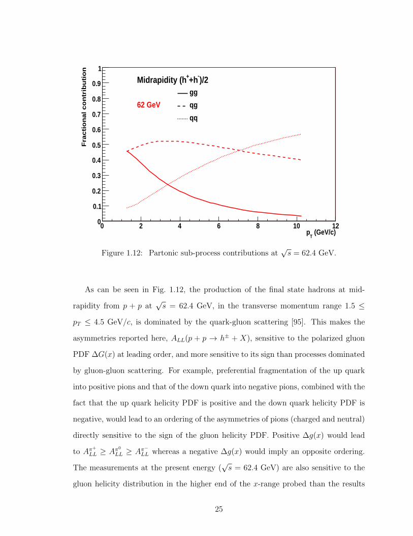
Figure 1.12: Partonic sub-process contributions at√s = 62.4 GeV.
As can be seen in Fig. 1.12, the production of the final state hadrons at mid-
rapidity from p + p at√s = 62.4 GeV, in the transverse momentum range 1.5 ≤
pT ≤ 4.5 GeV/c, is dominated by the quark-gluon scattering [95]. This makes the
asymmetries reported here, ALL(p + p → h± + X), sensitive to the polarized gluon
PDF ∆G(x) at leading order, and more sensitive to its sign than processes dominated
by gluon-gluon scattering. For example, preferential fragmentation of the up quark
into positive pions and that of the down quark into negative pions, combined with the
fact that the up quark helicity PDF is positive and the down quark helicity PDF is
negative, would lead to an ordering of the asymmetries of pions (charged and neutral)
directly sensitive to the sign of the gluon helicity PDF. Positive ∆g(x) would lead
to Aπ+
LL ≥ Aπ0
LL ≥ Aπ−LL whereas a negative ∆g(x) would imply an opposite ordering.
The measurements at the present energy (√s = 62.4 GeV) are also sensitive to the
gluon helicity distribution in the higher end of the x-range probed than the results
25

from other available energies (√s = 200, 500 GeV) at RHIC as xT = 2pT/
√s (as
can be seen from Figures 1.13 and 1.14). These results can be combined with data
from polarized collider and fixed target experiments in a global analysis to reduce
uncertainties on the gluon helicity distribution [59, 60].
Figure 1.13: Bjorken x range probed for√s = 62.4 GeV.
26

Figure 1.14: Bjorken x range probed for other RHIC energies.
27
CHAPTER 2
ACCELERATOR AND DETECTORS
The Relativistic Heavy-Ion Collider (RHIC) at Brookhaven National Laboratory
(BNL) is a unique facility to study proton spin structure by colliding two polarized
proton beams or study the state of matter in heavy ion (d+Au, Cu+Cu, Au+Au)
collisions. Most prominent of the collaborations at RHIC are : BRAHMS, PHENIX,
PHOBOS and STAR. PHOBOS was decommissioned in 2005 and BRAHMS com-
pleted data taking in June, 2006.
2.1 Polarized Protons at RHIC
The Relativistic Heavy-Ion Collider (RHIC) at Brookhaven National Laboratory
(BNL) on Long Island, New York, is the accelerator facility built for the study of the
state of matter at very high temperature through collisions of heavy ions (d + Au,
Cu + Cu, Au + Au) and for the study of the spin structure of the proton using
the collisions of polarized p + p. RHIC is the only polarized p + p collider in the
world, providing a unique opportunity for studying the proton spin structure. Each
of the two storage rings at the accelerator is 3.8 km in circumference and there
are six interaction points (IPs) for beam collisions (Fig. 2.1). There have been four
different experiments at four of these IP’s in the recent times : BRAHMES, PHENIX,
PHOBOS and STAR. A detailed description of the RHIC as a polarized proton collider
can be found in [34].
At RHIC, the design luminosity for the polarized p+p is 2×1032cm−2s−1 and the
design polarization for the proton beams is 70%. A maximum of 120 proton bunches
28
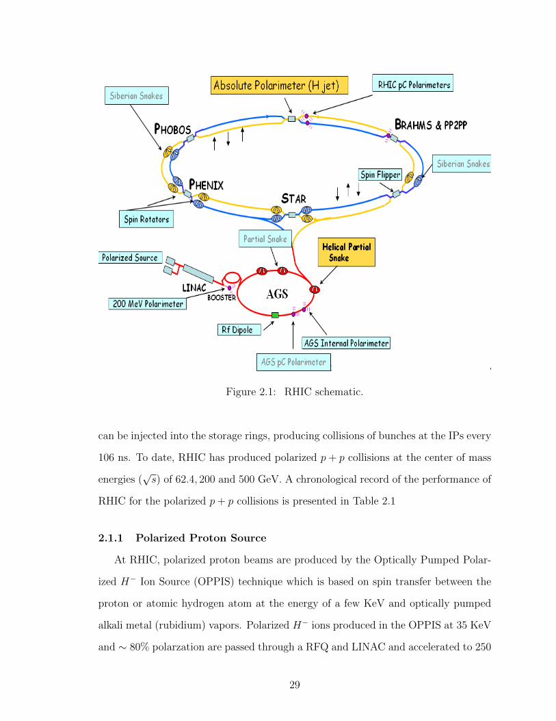
Figure 2.1: RHIC schematic.
can be injected into the storage rings, producing collisions of bunches at the IPs every
106 ns. To date, RHIC has produced polarized p+ p collisions at the center of mass
energies (√s) of 62.4, 200 and 500 GeV. A chronological record of the performance of
RHIC for the polarized p+ p collisions is presented in Table 2.1
2.1.1 Polarized Proton Source
At RHIC, polarized proton beams are produced by the Optically Pumped Polar-
ized H− Ion Source (OPPIS) technique which is based on spin transfer between the
proton or atomic hydrogen atom at the energy of a few KeV and optically pumped
alkali metal (rubidium) vapors. Polarized H− ions produced in the OPPIS at 35 KeV
and ∼ 80% polarzation are passed through a RFQ and LINAC and accelerated to 250
29

Year Beam energy Delivered luminosity Average store polarizationGeV b−1
2002 100.0 1.4 p 14 %2003 100.0 5.5 p 34 %2004 100.0 7.1 p 46 %2005 100.0 29.5 p 47 %2006 100.0 88.6 p 55 %
31.2 1.05 p 50 %2008 100.0 38.4 p 44 %2009 250.0 110 p 34 %
100.0 115 p 56 %2011 250.0 166 p 48 %
Table 2.1: A list of performance of RHIC in polarized p+ p collisions over the years.
MeV with 50% efficiency. Next the beam is passed through to a booster ring where
it is accelerated to ∼ 2 GeV. Proton bunches from the booster are injected into the
Alternating Gradient Synchroton (AGS) and accelerated to about 25 GeV. Maintain-
ing the polarization throughout the acceleration in the AGS is a difficult proposition
since the beams undergo various depolarizing effects e.g. matching of the betatron
frequency with spin precession frequency and horizontal magnetic field present in the
accelerator. To reduce the depolarizing effects, a device called the ‘Siberian Snake’ -
described in the following Sect. 2.1.2 - is implemented. However, due to the lack of
space, only partial (5%) snakes are used in the AGS. The addition of another 15%
‘cold snake’ [90] in 2005 significantly improved beam polarizations in the subsequent
years.
2.1.2 Depolarizing Effects and the Siberian Snake
For a proton with charge e and momentum ~p moving through a magnetic field, the
equations of motion of the proton and its spin vector in its instantaneous rest frame
are described by the Lorentz equation and the Thomas-BMT equation respectively :
d~p
dt= − e
mγ
~B⊥
× ~p, (2.1)
30
d~s
dt= − e
mγ(1 + γG) ~B⊥ + (1 +G) ~B‖ × ~s, (2.2)
where ~B⊥ and ~B‖ are the components of the magnetic field in perpendicular and
parallel to the momentum respectively, γ is the relativistic boost E/m and G is the
anomalous magnetic moment of the proton. For high energy protons (large γ), the ~B⊥
term dominates. For highly energetic protons, therefore, the spin rotates γG times
faster compared to the motion of the proton (orbital motion). This number is termed
as ‘spin tune’ νsp.
If the beam encounters any perturbing effect matching the frequency of the spin
precession, resonances occur, amplifying the depolarizing effect. Depolarization reso-
nance effects on the accelerating proton beams are usually from two sources : intrinsic
effects and imperfections of magnetic fields. Intrinsic depolarizing effects occur when
the betatron oscillation frequency matches the spin precession tune νsp. The second
type of depolarization comes into effect when the rotating polarized beam is affected
by an imperfection in the (focusing) magnetic field each revolution and the frequency
of the imperfection in the field matches the spin tune. In such cases, the spin is in the
same phase each time the protons pass through the depolarizing field. The matching
of frequencies of depolarizing effects with that of the beam rotation on the resonance
effects are demonstrated in the cartoon Fig. 2.2.
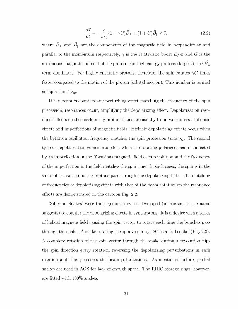
‘Siberian Snakes’ were the ingenious devices developed (in Russia, as the name
suggests) to counter the depolarizing effects in synchrotons. It is a device with a series
of helical magnets field causing the spin vector to rotate each time the bunches pass
through the snake. A snake rotating the spin vector by 180 is a ‘full snake’ (Fig. 2.3).
A complete rotation of the spin vector through the snake during a revolution flips
the spin direction every rotation, reversing the depolarizing perturbations in each
rotation and thus preserves the beam polarizations. As mentioned before, partial
snakes are used in AGS for lack of enough space. The RHIC storage rings, however,
are fitted with 100% snakes.
31

Figure 2.2: Cartoon showing amplified depolarizing effect with successive rotationsof the beam for resonance.
Figure 2.3: Diagram of the magnetic field of a full siberian snake rotating the spindirection by 180.
2.1.3 Accelerator
Polarized proton bunches at 25 GeV from AGS are injected into the accelera-
tor/storage rings where they are further accelerated to the required collision energy
(e.g. 31.2, 100, 250 GeV). A group of proton bunches (120 at most) in each ring is
termed as a ‘fill’ and are tagged with a number. Each fill is kept rotating in the storage
32
ring (and colliding at the IPs) for typically 7−8 hours. At RHIC, the proton bunches
in a ring are given a set pattern of successive spin configurations in any particular fill.
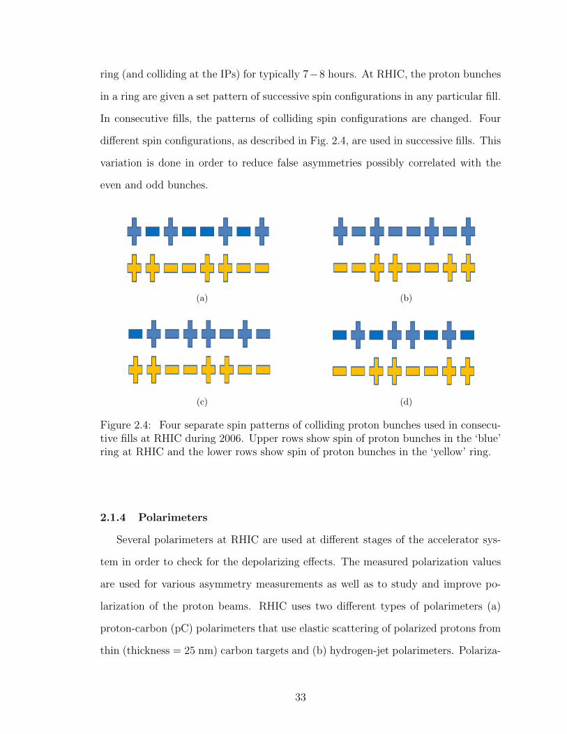
In consecutive fills, the patterns of colliding spin configurations are changed. Four
different spin configurations, as described in Fig. 2.4, are used in successive fills. This
variation is done in order to reduce false asymmetries possibly correlated with the
even and odd bunches.
(a) (b)
(c) (d)
Figure 2.4: Four separate spin patterns of colliding proton bunches used in consecu-tive fills at RHIC during 2006. Upper rows show spin of proton bunches in the ‘blue’ring at RHIC and the lower rows show spin of proton bunches in the ‘yellow’ ring.
2.1.4 Polarimeters
Several polarimeters at RHIC are used at different stages of the accelerator sys-
tem in order to check for the depolarizing effects. The measured polarization values
are used for various asymmetry measurements as well as to study and improve po-
larization of the proton beams. RHIC uses two different types of polarimeters (a)
proton-carbon (pC) polarimeters that use elastic scattering of polarized protons from
thin (thickness = 25 nm) carbon targets and (b) hydrogen-jet polarimeters. Polariza-
33

tion of the beams are determined by measuring the left-right asymmetries of scattered
particles :
Pbeam =1
AN
(Nright −Nleft
Nright +Nleft
),
=ε
AN, (2.3)
where ε is the raw asymmetry and the analyzing power AN is given by :
AN =1
Pbeam
(N↑ −N↓N↑ +N↓
), (2.4)
the subscripts denoting the two possible spin configurations of the polarized beam.
The analyzing power is measured from other experiments (in the case of the pC
polarimeter) and the from the scattering of the recoil of the target (in case of the
H-jet polarimeters).
In the first technique mentioned, the recoil carbons are detected using silicon
sensors. At the relevant energy scale, interference occurs between the electromagnetic
(QED) and hard (QCD) scattering amplitudes and these method of polarimetry are
therefore termed as the Coulomb-Nuclear Interference (CNI) techniques. Each of
the RHIC rings and AGS uses a pC polarimeter each for polarization measurements.
Polarization measurements by pC polarimeters are very fast (∼ million events every
second), however, the analyzing power ApCN used for these measurements was obtained
from the E950 experiment [35] at AGS and it had a large (∼ 30%) uncertainty. The
pC polarimeter techniques and measurements are described in detail in [84].
The fast measurements at the pC polarimeters are calibrated by the second type of
polarimeters. About 96% polarized hydrogen gas jets are ionized and passed through
the beam pipe. The elastic scattering of protons are used to measure recoil protons by
silicon strip sensors. In this case however, the analyzing power is measured by using
the precisely (within 2%) known values of the target polarization and the asymmetry
34

of the target scattering (AN = εtarget/Ptarget). The same analyzing power is used
with the measured beam scattering asymmetry to calculate beam polarization. The
measurements by H-Jet polarimeters are slow and it takes several hours to gather
enough data points for the required accuracy. More details of this techniques and the
H-jet measurements can be found in [85].
2.1.5 Spin Rotator
In the RHIC storage ring, the polarized protons have the spin vector in the ver-
tical direction as it is the stable configuration at RHIC (siberian snakes help reduce
depolarization effects with a vertical spin direction). At interaction points however,
the experiments require different spin directions (vertical, radial or longitudinal) for
various asymmetry measurements. A set of four helical dipole magnets (one each on
both sides of the nominal interaction region for each RHIC ring) are used at the IP’s
for PHENIX and STAR experiments for the purpose of rotating the spin direction
of the colliding proton bunches to the desired direction and bringing it back to the
stable vertical direction before putting the bunches back in the RHIC rings. Detailed
description of the spin rotators can be found in this comprehensive review [34].
2.2 PHENIX Detectors
The PHENIX experiment [22] was designed keeping in view photon, electron and
muon measurements with high rate data collection and high resolution of energy/mass
measurement and particle identification. In particle physics experiments, the scat-
tering angle with respect to the beam direction is an important quantity and often
certain types of interactions of interest produce particles in certain zones of this
angle. Pseudo-rapidity (η = 12
ln(
∣∣∣→p ∣∣∣+pL∣∣∣→p ∣∣∣−pL ) = − ln(tan θ2)), a function of the angle, is
used to parameterize experimental results or describe detector designs. The PHENIX
detector system consists of two central arm spectrometers at mid-rapidity and two
35

spectrometers at forward rapidity regions for tracking and identifying muons specifi-
cally.
Each of the central arm spectrometers has an acceptance covering a pseudo-
rapidity range of |η| ≤ 0.35 and δφ = 90 in azimuth. Central arm detectors are
essentially for tracking and identifying charged particles and detection and energy
measurements of photons. The tracking system consists of drift chambers (DC) and
pad chambers (PC). The ring imaging Cherenkov detector (RICH) and time-of-flight
(TOF) provide charged particle identification and the electromagnetic calorimeter
(EMCal) provide energy measurements of photons and electrons. PHENIX detectors
during the 2006 run at RHIC are shown in Fig. 2.5
2.2.1 Luminosity Detectors
PHENIX uses the two global detectors, a pair of beam beam counter (BBC) and
a pair of zero degree calorimeter (ZDC) on both sides of the interaction region [22].
The BBC is used for (a) triggering, (b) determining the event vertex along beam
direction and (c) for timing calibrating used in the Time of Flight calculations. Each
side of the BBC is composed of 64 photomultiplier tubes (PMT). Each of the one-
inch diameter mesh-dynode photomultiplier tubes is equipped with a 3 cm quartz
in front of the PMT used as a Cherenkov radiator (Fig. 2.6). Each BBC array is
placed 144 cm from the nominal interaction center and about 1 cm from the beam
pipe. The BBC array has an inner diameter of ∼ 10 cm and outer diameter ∼ 30 cm.
The BBCs cover a pseudo-rapidity range on 3.0 ≤ |η| ≤ 3.9 and complete azimuthal
coverage. BBC has a timing resolution of 52± 4 ps for a single PMT. A laser signal
is simultaneously delivered to Time-of-Flight detector, Electro-Magnetic Calorimeter
and each individual BBC elements to monitor and calibrate the timing information.
A well monitored air flow system is used to cool the BBC system constantly. Timing
information for each BBC is calculated as :
36

West
South Side View
Beam View
PHENIX Detector
North
East
MuTr
MuID MuID FCal
HBD
HBD
PbSc PbSc
PbSc PbSc
PbSc PbGl
PbSc PbGl
TOF
PC1 PC1
PC3
PC2
Central Magnet
Central Magnet
North M
uon Mag
net South Muon M
agnet
TEC PC3
BB
BB
MPC
MPC
BB
RICH RICH
DC DC
ZDC/SMD ZDC/SMD
Aerogel
FCal
Figure 2.5: PHENIX detector during 2006 data taking period.
Tcorr = Traw − Toffset − C/√Q, (2.5)
where Traw is the uncorrected arrival time of the signal, Toffset is the time offset
in each individual BBC element, Q is the measured charge of the signal and C is
the coefficient of time walk (determined by minimizing δti = TN/S − ti for all BBC
elements).
For the dataset used for the present analysis, a BBC local level 1 trigger (minimum
bias trigger) was defined as a coincidence of at least one PMT hit on both sides of
37

Figure 2.6: (a) Single Beam Beam Counter consisting of mesh-dynode photo-multiplier tube on a 3 cm quartz radiator and (b) BBC array comprising 64 units. [38]
the BBC. The hit times of all PMTs on one side is averaged and the average hit time
from the two sides are used to calculate the event vertex position zvtx :
zvtx = c (TS − TN) /2, (2.6)
where c is the velocity of the particles and TS, TN are the average hit times in the
two sides of the BBC. The time zero t0 of the collision events used for time-of-flight
calculations is given by t0 = (TS + TN) /2. With the given BBC timing resolution,
the spatial resolution of zvtx measurement is ∼ 5 cm for online measurements and
∼ 2 cm for offline measurements. BBC’s are used for luminosity counts for the cross
38

section measurements (counts are normalized by the process cross section seen by the
BBC trigger, termed as ‘BBC cross section’) and for the determination of relative
luminosities for asymmetry measurements (using the scaler data of BBC triggered
event counts) at PHENIX.
One aspect of averaging hit times from all PMT’s in each arm is that BBC is
blind to the multiple collision events in a single bunch crossing. This creates a mis-
calculated luminosity measurement. For the 2006 run, with the given beam intensities,
the multiple collision rates were small ∼ 5% and the effect on relative luminosity
measurement is negligible. For later years of data, the effect may be significant for
the desired precision of asymmetry measurements (∼ 10−4).
ZDC’s are hadronic calorimeters used for forward neutron tagging at PHENIX.
The ZDC’s are located at ±18 m from the nominal interaction center and cover a
cone of 2 mrad with a pseudo-rapidity range of η ≥ 6. ZDC has a timing resolution of
∼ 150 ps and resulting spatial resolution for the vertex determination using ZDC is
∼ 30 cm. For cross section measurement, ZDC triggered data is used in conjunction
with BBC triggered data to properly determine the luminosity normalization constant
σBBC (BBC cross section). The comparison of BBC triggered data in coincidence with
ZDC triggered data gives the z-dependence of the triggered events. For asymmetry
measurements, ZDC triggered data is used for the comparison of BBC triggered data
in order to determine the systematic uncertainty on the relative luminosity R.
2.2.2 PHENIX Magnets
The PHENIX magnet system [43] has three parts made of iron yokes and water-
cooled copper coils, the Central Magnet (CM) and north and south Muon Magnets
(MMN and MMS). The Central Magnet provides an axially symmetric field around
the interaction vertex for the entire azimuth with∫Bdl = 0.78 T.m. This field causes
the charged particles to bend in a plane perpendicular to the beam axis. The bending
39

angles, measured at Drift Chamber, provide measurements of particle momenta. For
the 2006 run, the ++ configuration was used for the central magnet (Fig. 2.7).
(a) ++ (b) +−
Figure 2.7: PHENIX magnets filed lines with (a) Central Magnet in ++ configurationand (b) Central Magnet in +− configuration.
2.2.3 Tracking Detectors
Outside the axial field of the PHENIX central magnet, each central arm has a DC
and layers of PC that are used for tracking charged particles [22, 21]. The PHENIX
DCs are cylindrically shaped and located in the region from 2 m to 2.4 m from the
beam axis z and 2 m wide along z. Each drift chamber measures the charged particle
tracks in the azimuthal (r−φ) direction and determine its transverse momentum pT .
The transverse momenta, along with the polar angle θ information from the PC1
hits, are used to calculate the total momentum p.
40

2.2.3.1 Drift Chambers
The DC system consists of two independent wire chambers filled with a gas mix-
ture (49.7% Ar + 49.7% Ethane + 1% C2H5OH) located in the east and west arms.
The volume of each detector is confined by a cyndrical titanium frame (Fig. 2.8).
Each frame in a single arm is divided in the azimuthal direction into 20 equal sectors
of 4.5 each. Each such sector consists of six modeules of wires stacked in radial
direction : two sets of wires (X1,X2) parallel to the beam direction and two pairs
of (U1,V1 and U2,V2) stereo wire at a 6 angle with respect to the X wires. Each
module contains 4 anode planes and 4 cathode planes forming cells of 2−2.5 cm drift
lengths in the φ direction. X wires are used for the precise measurements of tracks
in the r − φ plane and the U, V wires are used to measure the z coordinates of the
tracks. The stereo angle is chosen by matching the z resolution of the pad chambers
to minimize ambiguity of track matching with hits in the DC and PC.
Each of the X cells contain 12 anode wires and each of the U, V cells contain 4
anode wires. The wire configuration in each sector of the DC is shown in Fig. 2.9.
The anode wires are separated by Potential wires (P) and surrounded by Gate (G)
and Back (B) wires. The P wires form a strong electrical field. The G wires limit the
track sample length to ∼ 3 mm and help minimizing the time spread of the drifting
electrons from a single track. The B wires are at low potential and they terminate
most of the drift lines from its side, thereby reducing the left-right ambiguity. The
drift chambers are designed to have (a) single wire resolution better than 150 µm
in r − φ, (b) single wire two track separation better than 1.5 mm, (c) single wire
efficiency 99% and (d) a spatial resolution in the z direction better than 2 mm.
2.2.3.2 Pad Chambers
The pad chambers are multi-wire proportional chambers with a single plane of
anode wires inside a gas volume bound by two cathode planes. One of the cathodes
41

Figure 2.8: Titanium frame defining the DC volume [21].
is a solid plane and the other is segmented into pixels. A cell contains three pixels
and an avalanche must be traced by all three pixels to have a valid hit in the cell
(Fig. 2.10). An array of 9 connected pixels is named ‘pad’. A cell area of 8.4×8.4 mm2
results in a position resolution of 1.7 mm in the z direction. There are two layers of
PC in the east arm and three in the west. To maintain the same angular resolution,
further layers of pad chambers have larger cell sizes e.g. cells in PC3 have four times
the area of cell in PC1 as PC3 is at twice the distance from beam axis as PC1.
PC1 in each arm (East and West) is composed of 8 separate chambers each of size
0.5 × 2 m2. Pad chamber hit information is used in conjunction with DC hits to
reduce ambiguity in the track reconstruction. Outermost layers of PC are used for
42

Figure 2.9: Wire configuration in the DC [21].
matching the projected tracks and the method is used to separate backgrounds from
charged hadron tracks. More on the track reconstruction at PHENIX using DC and
PC is discussed in Sect. 3.1 in the following chapter.
2.2.3.3 Drift Chamber Quality Analysis
Minimum bias triggered data was used to perform quality analysis of the DC. For
four quadrants of the detector (two sides of the nominal interaction center for each
of the East and West arms), track counts are plotted as a function of the variable
‘board’ (signifying 20 sectors of the DC) defined as :
43

Figure 2.10: The pad and pixel configuration (left). A cell is defined by three pixels(right). [21]
boardEast =3.72402− φ+ 0.008047× cosφ+ 0.87851
0.01963496(2.7)
boardWest =0.573231 + φ− 0.0046× cosφ+ 0.05721
0.01963496. (2.8)
Tracks are selected with similar requirements as for the final analysis (as discussed
in detail in Sect. 3.1). Events with vertices within 30 cm of the nominal interaction
center are selected. Best quality tracks are chosen with a matching window of 3σ in
the PC3dφ, PC3dz and variables for pT > 0.2 GeV/c.
Tracks are plotted in the α-board (α being the bending angle of tracks in the DC)
plane and dead or low-occupancy segments are determined as a function of bending
angle in DC α and board and are rejected for final comparisons (Figures 2.11, 2.12).
A run with the fewer problems and high performance is selected as a reference. The
ratio (r) of the number of tracks to the number of minimum-bias events is determined
44

for every run (segments of data taking period tagged with a number) and is compared
to the reference run across the 80 boards (4 quadrants each with 20 sectors/boards).
The ratio of the aforementioned quantity r for any run to that of the reference run
across the 80 boards are fitted with a constant value (sample plots : Figures. 2.13
and 2.14). The presence of the spikes in the ratio (w.r.t reference run) vs. board
plots indicate hot/faulty wires in DC. Presence of a few such bad wires can change
the fit quality (chi-square) and such run is rejected for analysis eventually after the
QA. The values of the constant parameter and the χ2 are used to determine any run
with abnormal performance and they are rejected for the final analysis.
board0 10 20 30 40 50 60 70 80
even
t cou
nts
0
2000
4000
6000
8000
10000
12000
Figure 2.11: Selected tracks as a function of board for the one half of the detectorin the East arm.
During the 2006 RHIC run, a large segment of the drift chamber in the west
arm was unavailable for data taking due to some dead/torn wires as can be seen in
Fig. 2.12, resulting in a low performance (< 50%) in the West arm and significant
loss of statistics. The segments were mended for the runs in the subsequest years.
45

board0 10 20 30 40 50 60 70 80
even
t cou
nts
0
2000
4000
6000
8000
10000
12000
Figure 2.12: Selected tracks as a function of board for the one half of the detectorin the West arm.
Figure 2.13: Ratio of normalized (by number of minimum bias events) tracks as afunction of board for the one half of the detector in the East arm.
2.2.4 Cherenkov Detectors
Placed after the DC and PC, a ring imaging Cherenkov (or Cherenkov) detector
(RICH) [33] is used for electron identification. The RICH uses CO2 at atmospheric
46

Figure 2.14: Ratio of normalized (by number of minimum bias events) tracks as afunction of board for the one half of the detector in the West arm.
pressure as a radiator, with a momentum threshold of 17 MeV/c for e±. It is pri-
marily used for identifying e±. Pion threshold for firing RICH is 4.65 GeV/c and in
conjunction with the EMCal, it provides e/π separation.
The Hadron Blind Detector (HBD, commissioned for one Arm only for the 2006
run) is a windowless triple gas electron multiplier (GEM) Cherenkov detector [33]. It
uses CF4 as the radiator gas with the pion threshold ∼ 4 GeV/c. The HBD is placed
near the beam pipe (50 − 60 cm) in the magnetic field free region. It uses a reverse
bias (voltage) to repel ionization from hadrons below the threshold (‘hadron blind’)
and is sensitive to photo-electrons from Cherenkov light only.
2.2.5 Particle ID Detectors
TOF detector uses the time of flight of particles from the collision vertex to the
detector in conjunction with the reconstructed track information to identify charged
particles. The detector had a small acceptance in 2006 (almost one-fourth of the
Central Arms). A description can be found in [33]. Time Expansion Chamber (TEC)
47

and Aerogel (small acceptance) are PID detectors that use energy loss (−dEdx
) of
particles in the material to identify charged particles.
2.2.6 Electromagnetic Calorimeter
The outermost component of the central arm spectrometers is the electromagnetic
calorimeter, located at r ∼ 5 m. It provides energy and position measurements of
e± and photons and also timing information. In the west arm, the calorimeter has
four sectors of lead-scintillator (PbSc) sampling calorimeters and in the east arm, two
sectors of PbSc along with two sectors of lead-glass (PbGl) Cherenkov calorimeters.
Each sector covers |η| ≤ 0.35 and δφ = 22.5. The PbSc sectors have energy resolution
of σE/E = 2.1%⊕ 8.1%/√E and timing resolution ∼ 300 ps. The PbGl sectors have
energy resolution of σE/E = 0.8% ⊕ 5.9%/√E and timing resolution ∼ 200 ps. A
more detailed description of the detector can found in [42].
2.2.7 Muon Arm Detectors
In the forward rapidity region the PHENIX Muon Arm [22] consists of Muon
Trackers (MuTr) and Muon-Identifier (MuID) Detectors. They cover an azimuth of
180 degrees and the pseudo-rapidity coverage is −2.25 < η < −1.15 for the south
arm and 1.15 < η < 2.44 for the north arm.
48

CHAPTER 3
DATA SELECTION, HADRON TRACK CRITERIA ANDBACKGROUNDS
3.1 Data Set
We analyzed proton-proton collision data taken at RHIC during 2006. In 2006,
RHIC operated with two different beam energies of 100 and 32.2 GeV (center of mass
energies of 200 and 64.4 GeV). The ten days of 62.4 GeV data were only a small sub-
set of the entire data from 2006. We analyzed data corresponding to an integrated
luminosity of 15.6 nb−1 (∼ 214 Million events, including both transverse and lon-
gitudinal polarization) for cross section measurement and 11.9 nb−1 (∼ 163 Million
events, longitudinally polarized) for asymmetry measurement. Analyzed events were
triggered by requiring the coincidence of at least one photo-tube hit on both sides of
the BBC (Minimum Bias trigger). This particular choice of trigger avoids the bias of
detection (introduced by the detectors associated with the triggers) towards different
hadron species. Event vertices were determined by using the differences of average
hit times in the north and south end of the BBC. For these analyses, event vertices
were chosen to be within 30 cm of the nominal interaction center to avoid collision of
particles with the Central Magnet.
From a p + p scattering event in the collision of a pair of proton bunches at the
interaction region, particles spread in different directions. For the hard processes
that we are interested in, we looked for the final state particles with high enough
transverse momentum and going to the PHENIX Central Arm detectors. DC and
PC1 in Central Arms, in conjunction with the event vertex information, are used
49

to reconstruct charged tracks. Track reconstruction is done separately in the bend
plane (r − φ plane) (Fig. 3.1) and the non-bend plane (r − z plane) (Fig. 3.2). In
the r − φ plane, reconstruction is done using the ‘Combinatorial Hough Transform’
technique in which any pair of hits can be mapped to a point in a space defined
by the azimuthal angle φ and track bending angle α. Assuming tracks are straight
lines within DC (negligible residual magnetic field after DC), all hit pairs associated
with a track should have the same (φ, α) and the mapping therefore will form a local
maxima in the φ−α phase space. Reconstruction in the bend plane determines the φ
and α of the tracks. The momentum of the charged particle is then calculated using
the bending angle α of the track measured in DC.
α ' K1
p, (3.1)
where K1 is the magnetic field integral ∼ 101 mrad GeV/c. Using this initial estimate
of the momentum, the final value is calculated from a pre-determined four dimensional
grid f(p, r, θ0, zvtx), where p is the initial estimate, r is the radius at which the field
integral is calculated, θ0 is the polar angle of the track at the vertex and zvtx is the
vertex position along the beam direction.
After the bend-plane, reconstruction is done in the non-bend plane. PC1 hit posi-
tion and event vertex zvtx determined by BBC were used to determine the direction of
the track and DC wire hits are associated with the track within a ±5 cm window. For
more than one possible PC1 hit, the number of DC hits are maximized to determine
the unique choice. The polar angle θ is determined from the reconstruction in the
r − z plane.
3.1.1 Beam-Shift Calibration
In the tracking algorithm, the momentum of a particle is estimated from the bend-
ing angle α (deviation of the track from an infinite momentum track from same vertex
50

Figure 3.1: Track reconstruction in the bend (azimuthal) plane at PHENIX.
and hitting the same point at the reference radius in Drift Chamber) as described in
Sect. 3.1. Measurement of the bending angle is sensitive to the precise calibration of
the position of the DC and the beam. If there is a shift of the beam or the DC arms
relative to the coordinate system, the measurement of angle α acquires an offset:
δα =δX × sinφ
RDC
+δY × cosφ
RDC
, (3.2)
where φ is the azimuthal angle and RDC is the reference radius in DC (220 cm from
ideal beam axis). This offset in angle is translated as an offset in the measured
momenta of the tracks. Using the time of flight (T ) of particles to the east arm of the
high resolution Time of Flight (TOF) detector in conjunction with the path length
(L) and the momentum (p) from the reconstruction model, the squared mass (m2) of
the particles are calculated.
51

Figure 3.2: Track reconstruction in the non-bend plane at PHENIX.
m2 = p2
(cT
L
2
+ 1
). (3.3)
In the mass-squared distribution of protons, a splitting is observed between protons
and antiprotons. This arises because the momentum shift due to the offset in the
bending angle (δα) affects different charged particles in different ways (increasing
measured momentum of one charge while decreasing the measured momentum of the
other). To extract the magnitude of the shifts (of beam or DC), parameters in Eq. 3.2
are varied to match the proton and anti-proton mass-square peaks. We estimated an
x-offset of 0.1 cm in the East Arm, an x-offset of −0.28 cm in the West Arm and
a y-offset of 0.2 cm. The proton (and/or antiproton) squared mass peak values
are compared to the standard particle data group accepted value (0.88 GeV2/c2) to
extract the ‘momentum scale correction factor’. The scale factor was determined to be
52
1.01 with 1% uncertainty. All reconstructed momentum measurements were corrected
for the beam offsets and were scaled appropriately to obtain final momentum values.
3.1.2 Selection Criteria
Along with the trigger choice and event vertex cut, several other conditions were
applied to the reconstructed track variables to select final state hadrons generated
from the p + p collisions. After the reconstruction, tracks are projected on PC3 and
the distribution of actual hits in the detector around the projected hits are matched.
The deviations of actual hits from the projected positions in the φ − z plane are
called matching variables. We impose selection cuts on the distribution of matching
variables ‘PC3dφ’ (sample plot in Fig. 3.3) and ‘PC3dz’ (sample plot in Fig. 3.4) in
order to select the hadrons produced from the collision event (‘signal’). Hadron track
selection criteria used for the analysis are listed below. We require tracks with
• an offline cut of 30 cm on the measured vertex position on both sides of the in-
teraction center to make sure that tracks do not collide with the central magnets
and produce secondary debris from conversions.
• transverse momentum range 0.5 ≤ pT ≤ 4.5 GeV/c,
• −75 ≤ zed ≤ 75 cm, where ‘zed’ is the hit position along beam direction in DC
reference radius 2.2 m.
• RICH veto (to eliminate electron tracks) as pions, the lightest hadron in the
mix, fires RICH at pT = 4.7 GeV/c and electrons fire RICH at pT ∼ 17 MeV/c,
therefore a requirement that RICH does not fire (‘veto’) eliminates e+, e− back-
ground tracks.
• track ‘quality’ = 63 and 31, where ‘quality’ is a parameter from track recon-
struction algorithm denoting roughly how many and how well different detector
53
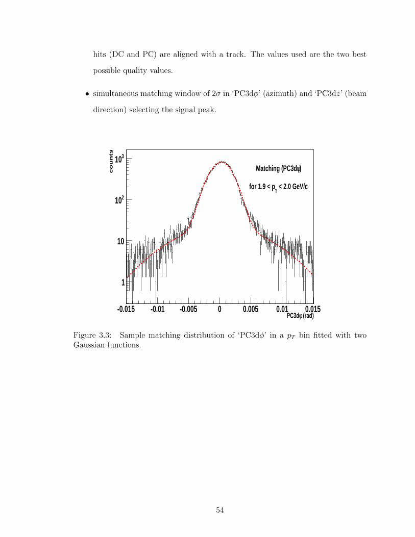
hits (DC and PC) are aligned with a track. The values used are the two best
possible quality values.
• simultaneous matching window of 2σ in ‘PC3dφ’ (azimuth) and ‘PC3dz’ (beam
direction) selecting the signal peak.
(rad)φPC3d-0.015 -0.01 -0.005 0 0.005 0.01 0.015
co
un
ts
1
10
210
310)φMatching (PC3d
< 2.0 GeV/cT
for 1.9 < p
Figure 3.3: Sample matching distribution of ‘PC3dφ’ in a pT bin fitted with twoGaussian functions.
54

pc3dz (cm)-30 -20 -10 0 10 20 30
co
un
ts
210
310
Matching (PC3dz)
< 2.5 GeV/cT
for 2.25 < p
Figure 3.4: Sample matching distribution of ‘PC3dz’ in a pT bin fitted with twoGaussian functions and a flat component.
55

3.2 Backgrounds
A substantial part of the possible backgrounds for the charged hadron tracks
are the electron and positron tracks (both directly from the vertex as well as from
conversion of photons) and they are eliminated very efficiently by the RICH veto
as electrons (and positrons) trigger RICH with very high efficiency(effectively 100%)
above pT > 17 MeV/c whereas pion - the lightest hadrons in the mix - fires RICH at
pT > 4.7 GeV/c. Another important source of the backgrounds is the weak decays of
the hadrons in flight.
Hadron decay backgrounds can be essentially categorized into two different groups:
• Backgrounds from the decays of short-lived particles : K0s , Λ (and heavier
hyperons) etc.
• Backgrounds from the decays of long-lived particles : π±, K±, K0l etc.
3.2.1 Long-lived Particle Decay
The largest contribution to the backgrounds comes from this category. These
particles have comparatively longer lifetimes (cτ ∼ 1 m) and they decay further
from the vertex and close to DC (e.g. conversions at the DC entrance window).
Decay products with significantly smaller mass than the parent get a relatively large
momentum kick and are spread over a wider range in the matching variables than
undecayed signal tracks. These are frequently mis-reconstructed as high-pT tracks. In
φ, the bending of the decay products in the residual magnetic field produce a smeared
double peaked distribution (positive particles on one side, negative on the other) and
in ‘z’, the distribution is mostly flat. Major constituents of these backgrounds are
muons (mostly from pion and kaon decays) and pions (mostly from kaon decays).
56

3.2.2 Short-lived Particle Decay
A second source of background is the feed-down backgrounds produced by weak
decays of mostly Λ particles close to the event vertex with apparent momenta close
to their true momenta and matching distributions peaked under the signal. These
particles have smaller lifetimes (cτ ∼ 1 cm or less) and therefore decay very close to
the vertex. Decay particles travel through most of the magnetic field. In ‘z’, they
have ∼ 50% wider distribution than primary particles, due to kicks from decay and
are mostly peaked (under the signal) in φ. Major constituents for these backgrounds
are the feeddown protons and antiprotons from decays of Λ and heavier hyperons.
3.2.3 Treatment of Backgrounds
One possible method of determining the contribution of backgrounds is to look
into the distribution of matching variables. For the long-lived particle decay, we can
estimate the fraction of background tracks using either ‘PC3dφ’ or ‘PC3dz’.
Using ‘PC3dφ’, the ratio of tracks within selection window (within ±2σ) to those
in the tail end (within 3σ-9σ) on one side (positive side for negative particles and neg-
ative side for positive particles) in the high pT > 6 GeVc bin (where mis-reconstructed
background tracks dominate the distribution) is calculated. This ratio is used to nor-
malize the the analogous ratio in all the relevant pT bins. Put in a concise form, it
gives us BG/S +BG within the selection window (±2σ) in matching variables for
signals :
BG
S +BG= (
3σ ≤ tracks ≤ 9σ
tracks < ±2σ)pT × (
tracks < ±2σ
3σ ≤ tracks ≤ 9σ)highpT
(3.4)
Using ‘PC3dz’ we can extract the background fraction in any pT bin by normaliz-
ing the background tracks within 5σ-15σ on both sides of the mean of the distribution
57

with the ratio of area under the ±2σ zone to the total area of 5σ-15σ zone on both
sides since the distribution is essentially flat. In a concise form:
BG
S +BG=
2(5σ ≤ tracks ≤ 15σ)
5(tracks < ±2σ). (3.5)
The background fraction from both variables are found to be quite similar and the
average of the two background fractions is used as the value for the analysis. The
difference between the two sets of values is used as the systematic uncertainty on the
background fraction. The measured background fractions are tabulated below (3.1).
These backgrounds are subtracted from the total detected tracks.
Feed-down contributions to the detected protons and antiprotons from weak de-
cays of Λ’s and heavier hyperons are estimated using input Λ and Λ spectra from
p + p measurements at√s = 63 GeV at ISR [40, 64] and at
√s = 62.4 GeV at
PHENIX with the GEANT3 [51] based simulation of the PHENIX detector. The
fractional contributions of the feed-down protons and antiprotons are independent
of pT above pT = 2 GeV/c and are close to 7 and 15% respectively. Below pT = 2
GeV/c the fractions increase with decreasing pT and are roughly 25 and 60% for pro-
tons and anti-protons respectively at pT = 0.5 GeV/c. Cross sections are corrected for
the feed-down backgrounds. For double helicity asymmetry measurements, however,
these background tracks fall under the signal peak in the distributions of matching
variables and cannot be separated and no knowledge of the asymmetries of these
backgrounds is available. For this reason, these category of backgrounds (∼ 1− 2%)
are not subtracted or corrected for in the asymmetry measurement presented here.
3.3 Hadron Species Fractions
Non-identified charged hadrons from p+ p at√s = 62.4 GeV/c consist mostly of
pions, kaons and protons and their anti-particles. For the purpose of applying several
58

pT Bin Background Systematic Background Systematicfraction (h+) error (h+) fraction (h−) error (h−)
0.50-0.60 0.05 0.03 0.01 0.030.60-0.70 0.04 0.02 0.01 0.030.70-0.80 0.04 0.02 0.01 0.030.80-0.90 0.03 0.02 0.01 0.030.90-1.00 0.03 0.01 0.01 0.021.00-1.10 0.03 0.01 0.01 0.021.10-1.20 0.03 0.01 0.01 0.021.20-1.30 0.03 0.01 0.01 0.021.30-1.40 0.03 0.01 0.01 0.011.40-1.50 0.03 0.01 0.01 0.011.50-1.60 0.03 0.01 0.01 0.011.60-1.70 0.03 0.01 0.01 0.011.70-1.80 0.03 0.01 0.01 0.011.80-1.90 0.03 0.01 0.02 0.011.90-2.00 0.03 0.01 0.02 0.012.00-2.25 0.03 0.01 0.03 0.012.25-2.50 0.04 0.01 0.03 0.012.50-2.75 0.05 0.01 0.04 0.012.75-3.00 0.06 0.01 0.06 0.023.00-3.25 0.09 0.01 0.09 0.023.25-3.50 0.11 0.03 0.11 0.023.50-3.75 0.17 0.01 0.17 0.033.75-4.00 0.22 0.03 0.23 0.024.00-4.50 0.34 0.02 0.31 0.11
Table 3.1: Background fractions for positive and negative hadrons in different pTbins.
species-dependent correction factors for our measurements, we need to understand the
relative contribution of different species in the hadron mix. The production fractions
were determined from identified hadron spectra from PHENIX [20] at√s = 62.4
GeV/c as well as earlier data from the ISR [40] at√s = 52.8 GeV/c and
√s = 63
GeV/c. We fit each the particle fractions as a function of pT with the function
(AeBpT +C) with the constraint that the sum of fractions of all particles(antiparticles)
is 1 using mostly PHENIX data at low pT and ISR data at high pT. For particles,
a compensating linear term (DpT ) is added to the kaon fraction fit and subtracted
59

from the proton fit. For antiparticles, a similar compensating term is added to the
negative pion fit and subtracted from the anti-proton fit. The species fractions and
the functional fits are shown in Figures 3.5 and 3.6.
0 2 4
Sp
ecie
s f
ractio
n
0
0.1
0.2
0.3
0.4
0.5
0.6
0.7
0.8
0.9
1
Positive Pion
0 2 4
Positive Kaon
PHENIX+ISR fit
PHENIX only fit
ISR only fit
PHENIX data
ISR data
(GeV/c)T
p0 2 4
Proton
Figure 3.5: Relative fraction of each species for positive hadrons.
Data from PHENIX identified measurement provide data points at the lower end
of the pT range. The limitations of pion-kaon separation effectively restricts the upper
end of the spectrum at ∼ 2 GeV/c. ISR data provide data for the higher end of the
pT range. But comparison at the lower pT range indicates a normalization difference
between the two data sets. We, therefore use the difference of cross sections measured
using species fractions from separate data sets as the systematic error on the mea-
surement of cross sections arising from the determination of the production fraction
of individual hadron species. The fit parameters (Table 3.2) are determined within a
few percent. Relative fractions from fit values are used to apply the corrections.
60

0 2 4
Specie
s fra
ction
0
0.1
0.2
0.3
0.4
0.5
0.6
0.7
0.8
0.9
1
Negative Pion
0 2 4
Negative Kaon
PHENIX+ISR fit
PHENIX only fit
ISR only fit
PHENIX data
ISR data
(GeV/c)T
p0 2 4
Antiproton
Figure 3.6: Relative fraction of each species for negative hadrons.
hadron A B C Dπ+ 1.02 -2.39 0.57 -K+ -0.53 -2.39 0.20 0.009p -0.49 -2.39 0.23 -0.009π− 1.17 -2.49 0.61 0.012K− -0.61 -2.49 0.20 -p− -0.56 -2.49 0.18 -0.012
Table 3.2: Parameters of the fit (AeBpT + C) to the relative fractions of differentspecies in the hadron mixture. See text for details.
61
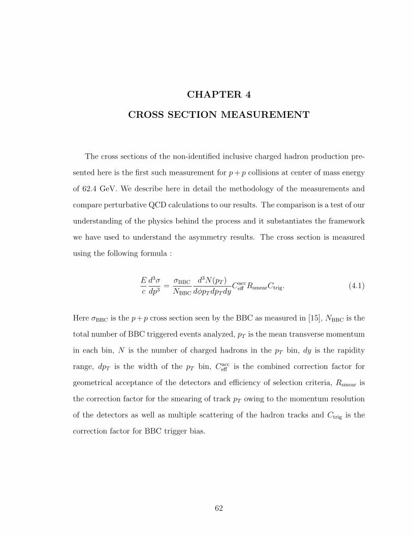
CHAPTER 4
CROSS SECTION MEASUREMENT
The cross sections of the non-identified inclusive charged hadron production pre-
sented here is the first such measurement for p+ p collisions at center of mass energy
of 62.4 GeV. We describe here in detail the methodology of the measurements and
compare perturbative QCD calculations to our results. The comparison is a test of our
understanding of the physics behind the process and it substantiates the framework
we have used to understand the asymmetry results. The cross section is measured
using the following formula :
E
c
d3σ
dp3=σBBC
NBBC
d3N(pT )
dφpTdpTdyCacc
eff RsmearCtrig. (4.1)
Here σBBC is the p+p cross section seen by the BBC as measured in [15], NBBC is the
total number of BBC triggered events analyzed, pT is the mean transverse momentum
in each bin, N is the number of charged hadrons in the pT bin, dy is the rapidity
range, dpT is the width of the pT bin, Cacceff is the combined correction factor for
geometrical acceptance of the detectors and efficiency of selection criteria, Rsmear is
the correction factor for the smearing of track pT owing to the momentum resolution
of the detectors as well as multiple scattering of the hadron tracks and Ctrig is the
correction factor for BBC trigger bias.
62

4.1 Corrections Factors Appropriate for the Detector
Various correction factors are applied to account for the geometry and the perfor-
mance of the detectors. The three major correction items are discussed in detail in
the following sections.
4.1.1 Acceptance of Detectors and Efficiency of Selection Cuts
To estimate the combined efficiency of the selection criteria and geometrical accep-
tance of the detector system, single particle Monte Carlo simulations are performed
and passed through the geant3 based detector configuration. It’s essential to look at
Cacceff for each separate particle species in the charged hadron mix as it can be affected
by the mass of each particle species and also the interactions and different decay
processes of each species. A Million of each of the charged hadron species (π, K,
p) and their antiparticles were generated, distributed uniformly in 2π azimuth, and
±0.5 of rapidity (y) range with a uniform distribution in transverse momentum range
of 0 ≤ pT ≤ 7.0 GeV/c. Particles were produced with a realistic vertex distribution
(typically Gaussian with an r.m.s of 50 cm truncated at ±30 cm) similar to that in
the data. The simulations take into account dead-maps for several detectors from the
period of time when the data was taken and were finally verified by comparing the
live and most efficient detector areas in both Monte Carlo and data.
Matching variables (‘PC3dφ’, ‘PC3dz’) of the positive and negative pions were
used for the calibrations for all species before we imposed the selection window as
pions were the bulk of the hadron mix and also because the variations for differ-
ent species were not significant for the purpose. Matching variable distributions in
each of the pT bins were fitted with the combination of a narrow Gaussian for the
signal (hadron tracks generated at the vertex) and a second wider Gaussian for the
background. The widths and means of the signal Gaussians were parameterized as a
function (AeBpT + C) of pT . In order to select hadrons from simulated events, a 2σ
63
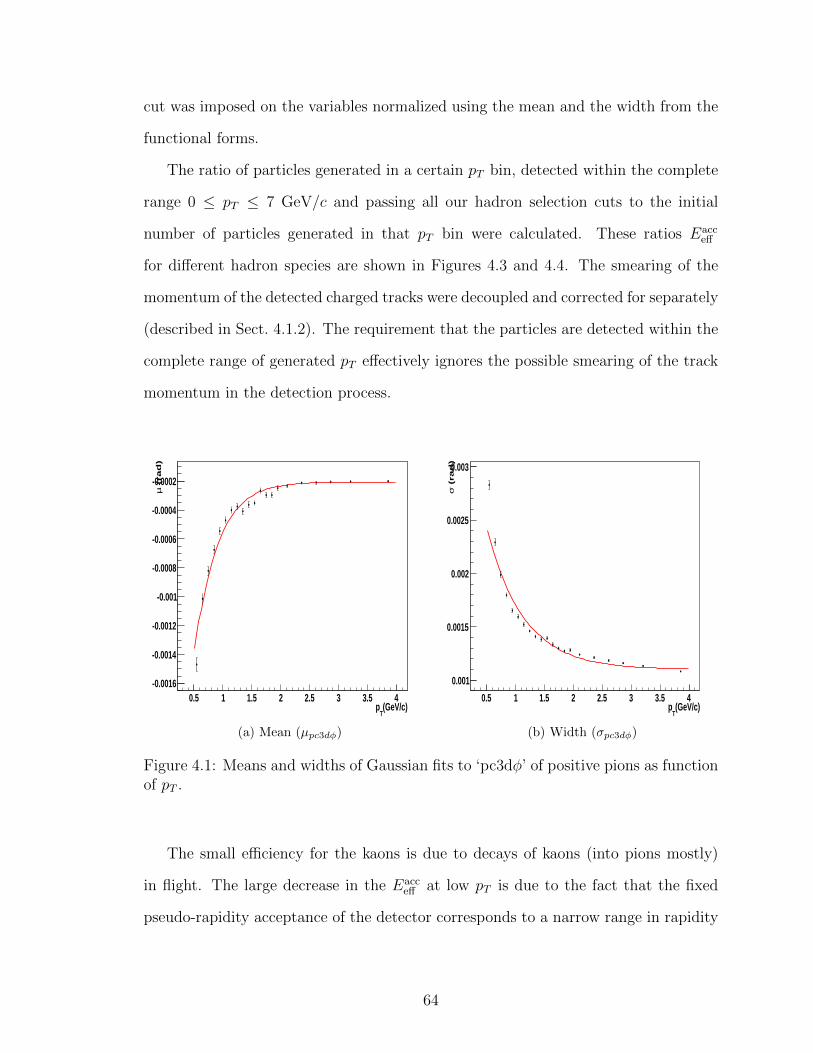
cut was imposed on the variables normalized using the mean and the width from the
functional forms.
The ratio of particles generated in a certain pT bin, detected within the complete
range 0 ≤ pT ≤ 7 GeV/c and passing all our hadron selection cuts to the initial
number of particles generated in that pT bin were calculated. These ratios Eacceff
for different hadron species are shown in Figures 4.3 and 4.4. The smearing of the
momentum of the detected charged tracks were decoupled and corrected for separately
(described in Sect. 4.1.2). The requirement that the particles are detected within the
complete range of generated pT effectively ignores the possible smearing of the track
momentum in the detection process.
(GeV/c)T
p0.5 1 1.5 2 2.5 3 3.5 4
(ra
d)
µ
-0.0016
-0.0014
-0.0012
-0.001
-0.0008
-0.0006
-0.0004
-0.0002
(a) Mean (µpc3dφ)
(GeV/c)T
p0.5 1 1.5 2 2.5 3 3.5 4
(ra
d)
σ
0.001
0.0015
0.002
0.0025
0.003
(b) Width (σpc3dφ)
Figure 4.1: Means and widths of Gaussian fits to ‘pc3dφ’ of positive pions as functionof pT .
The small efficiency for the kaons is due to decays of kaons (into pions mostly)
in flight. The large decrease in the Eacceff at low pT is due to the fact that the fixed
pseudo-rapidity acceptance of the detector corresponds to a narrow range in rapidity
64

(GeV/c)T
p0.5 1 1.5 2 2.5 3 3.5 4
(cm
)µ
-0.1
-0.05
0
0.05
0.1
(a) Mean (µpc3dz)
(GeV/c)T
p0.5 1 1.5 2 2.5 3 3.5 4
(c
m)
σ
2
2.1
2.2
2.3
2.4
2.5
(b) Width (µpc3dz)
Figure 4.2: Means and widths of Gaussian fits to ‘pc3dz’ of positive pions as functionof pT .
for smaller pT/m. The efficiencies were parameterized (AeBpT + C) as a function of
pT (Table 4.1) and fit values were used for the calculation of cross sections.
hadron A B Cπ+ -0.08 -1.8 1.453K+ -0.17 -0.97 1.280p -0.21 -1.54 1.428π− -0.07 -1.7 1.449K− -0.17 -1.01 1.276p− -0.21 -1.56 1.424
Table 4.1: Fit function parameters for the efficiency curves for different hadronspecies. See text in Sect. 4.1.1 for details.
As mentioned above, for the purpose of the verifying the MC simulation with
data, three of the largest and most efficient areas of the detector were chosen for
each of the quadrants (two sides of the nominal interaction center for each of the
two arms of detector systems). The ratio of the fractions of counts in the three
selected regions for each quadrant from data and simulation were calculated and the
65

(GeV/c)T
p0 0.5 1 1.5 2 2.5 3 3.5 4 4.5 5
eff
ac
cΕ
0
0.02
0.04
0.06
0.08
0.1
0.12
0.14
0.16
0.18
0.2
Positive Pion
Positive Kaon
Proton
Figure 4.3: Efficiency (includes geometrical acceptance, efficiency of detectors andefficiency of cuts), for positive hadrons.
weighted average (using the total count in each quadrant as the weights) was used
to scale the efficiencies from the simulation. The standard deviation was assigned as
the uncertainty of the ratio. The individual scale factors in each quadrant are listed
below (Table. 4.2) for positive and negative hadrons.
Positive:
hadrons East-North East-South West-North West-Southh+ 1.08± 0.13 1.08± 0.03 1.02± 0.07 1.10± 0.06h− 1.05± 0.09 1.04± 0.02 1.08± 0.04 1.16± 0.06
Table 4.2: Scale factors applied to Monte Carlo simulation to account for live detectorarea in each quadrant of the detector for positive and negative hadrons.
66

(GeV/c)T
p0 0.5 1 1.5 2 2.5 3 3.5 4 4.5 5
eff
ac
cΕ
0
0.02
0.04
0.06
0.08
0.1
0.12
0.14
0.16
0.18
0.2
Negative Pion
Negative Kaon
Antiproton
Figure 4.4: Efficiency (includes geometrical acceptance, efficiency of detectors andefficiency of cuts), for negative hadrons.
4.1.1.1 Applying The Correction
The correction factor Cacceff was applied according the relative fraction of each of
the species in the detected hadron mix. As described in detail in Sect. 3.3, the
production ratios of the hadron species are calculated fitting the identified hadron
data. Combined with these fractions fi for a species i, the relation between detected
yield Ydet and the corrected yield Ycor becomes :
Ycor ×∑i
fi(Eacceff )i = Ydet (4.2)
Ycor =Ydet∑
i fi(Eacceff )i
. (4.3)
The correction factor for acceptance and efficiency Cacceff = 1/
∑i fi(E
acceff )i for the
charged hadrons are shown in Figures 4.5 and 4.6.
67

(GeV/c)T
p0.5 1 1.5 2 2.5 3 3.5 4 4.5
eff
acc
C
7
7.5
8
8.5
9
9.5Positive Hadrons
Figure 4.5: Combined correction factor for the geometrical acceptance of the detectorand the efficiency of the selection criteria for positive hadrons.
4.1.2 Momentum Smearing and Correction
As mentioned in Sect. 4.1.1, the corrections due to effects of detectors were decou-
pled into two separate parts : (1) a correction term based on the combined detector
efficiency, geometrical acceptance and efficiency of our selection cuts and (2) a sep-
arate correction term that accounts for the uncertainty of the reconstructed hadron
tracks owing to the finite resolution arising from the angular resolution of DC and
multiple scattering of the tracks inside DC (more prominent for low pT tracks). An-
gular resolution in DC can be well approximated by a Gaussian distribution of width
∼ 0.9 mrad [22].
For the later correction, we started with a known spectrum of yield using ISR [40]
identified pion cross section. Pion spectra are fitted with a parameterization A(1 +
pTB
)2. Cross sections are converted in produced particle counts in pT bins and species
68

(GeV/c)T
p0.5 1 1.5 2 2.5 3 3.5 4 4.5
eff
acc
C
7
7.5
8
8.5
9 Negative Hadrons
Figure 4.6: Combined correction factor for the geometrical acceptance of the detectorand the efficiency of the selection criteria for negative hadrons.
fraction fi and efficiencies Eacceff are applied to get detected counts or ‘yields’ in each
bin. As a next step, all yields in the pT bins are converted in terms on α bins, where
bending angle α = K1/p, where K1 = 101 mrad GeV/c. Yield in each of the alpha
bins are distributed (smeared) according to a Gaussian around the mean alpha of the
bin with a width equal to the α-resolution δα. The value used for the total angular
resolution is :
δα = 0.9 + 0.007α, (4.4)
where the first term comes from angular resolution of Drift Chamber and the second
α-dependent term incorporates the effects of the multiple scattering which is more
prominent at low pT or high α. The values used are the same as used in previous
PHENIX results [12], the δp/p being converted to δα in this case.
69
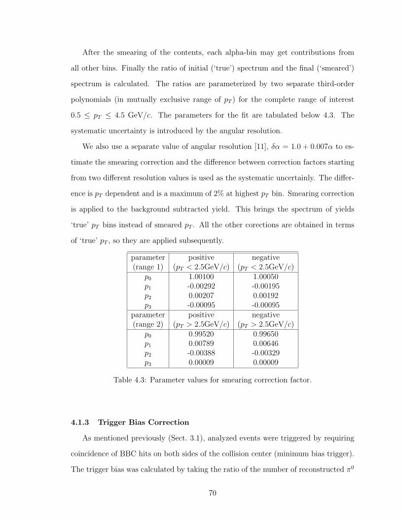
After the smearing of the contents, each alpha-bin may get contributions from
all other bins. Finally the ratio of initial (‘true’) spectrum and the final (‘smeared’)
spectrum is calculated. The ratios are parameterized by two separate third-order
polynomials (in mutually exclusive range of pT ) for the complete range of interest
0.5 ≤ pT ≤ 4.5 GeV/c. The parameters for the fit are tabulated below 4.3. The
systematic uncertainty is introduced by the angular resolution.
We also use a separate value of angular resolution [11], δα = 1.0 + 0.007α to es-
timate the smearing correction and the difference between correction factors starting
from two different resolution values is used as the systematic uncertainly. The differ-
ence is pT dependent and is a maximum of 2% at highest pT bin. Smearing correction
is applied to the background subtracted yield. This brings the spectrum of yields
‘true’ pT bins instead of smeared pT . All the other corections are obtained in terms
of ‘true’ pT , so they are applied subsequently.
parameter positive negative(range 1) (pT < 2.5GeV/c) (pT < 2.5GeV/c)
p0 1.00100 1.00050p1 -0.00292 -0.00195p2 0.00207 0.00192p3 -0.00095 -0.00095
parameter positive negative(range 2) (pT > 2.5GeV/c) (pT > 2.5GeV/c)
p0 0.99520 0.99650p1 0.00789 0.00646p2 -0.00388 -0.00329p3 0.00009 0.00009
Table 4.3: Parameter values for smearing correction factor.
4.1.3 Trigger Bias Correction
As mentioned previously (Sect. 3.1), analyzed events were triggered by requiring
coincidence of BBC hits on both sides of the collision center (minimum bias trigger).
The trigger bias was calculated by taking the ratio of the number of reconstructed π0
70

(GeV/c)T
p0 0.5 1 1.5 2 2.5 3 3.5 4 4.5 5
smea
rR
0.95
0.96
0.97
0.98
0.99
1
1.01
Figure 4.7: Correction factor for the momentum smearing of reconstructed tracks inthe detector. Figure shows fit to the ratio of the positive charged hadron spectrumin ‘true’ pT vs. that in the ‘smeared’ pT .
in the high pT photon triggered (EM calorimeter and RICH trigger) data with and
without requiring the coincidence of the minimum bias trigger [15]. The calculated
trigger bias is parameterized as a second order polynomial function of pT and the
parameterized values are used for the calculation of the cross sections. The trigger
bias as depicted in Fig. 4.8 shows a decrease towards the higher end of pT . This
effect is understood in terms of a deficit of the energy available to the forward (in
pseudo-rapidity) particles while producing high pT tracks in the mid-rapidity.
The trigger bias is parameterized as a non-linear function of pT as shown below.
The functional values are used to calculate cross section at various pT bins.
Etrigger =1
Ctrig
= a0 + a1pT + a2pT2,
71

where a0 = 0.4027± 0.0154,
a1 = 0.01966± 0.0109,
a2 = −0.00647± 0.0018.
0
0.05
0.10
0.15
0.20
0.25
0.30
0.35
0.40
0.45
0πf
(GeV/c)Tp
0 1 2 3 4 5 6 7 8
Figure 4.8: Parameterized efficiency of Minimum Bias trigger.
4.2 Luminosity Normalization and Cross Section Measure-
ment
4.2.1 Luminosity Normalization and Vernier Scan
The parameter σBBC is the part of the total process cross section available to the
BBC trigger (minimum bias trigger). It is estimated using various beam parameter
information (intensity of colliding bunches, frequency of collisions) and measurements
of transverse widths of the beams using the Vernier scan (Van der Meer scan) tech-
nique. For the data set discussed here, the measurements were done at PHENIX as
72

part of the neutral pion cross section and asymmetry measurements and discussed in
detail in [15]. The σBBC is defined as :
σBBC =RBBCmax
LmachineεBBC, (4.5)
where RBBCmax is the BBC triggered event rate at the maximal overlap of two beams, ε is
the efficiency of the BBC trigger (fraction of the collisions that falls within the vertex
region |zvtx| < 30 cm available to the trigger) and the delivered machine luminosity
Lmachine is defined as :
Lmachine = fNBNY
2πσxσy, (4.6)
where f is frequency of revolution (∼ 78 kHz) of proton bunches, NB, NY are the
intensity of two beams and σx, σy are the rms widths of the transverse beam profiles
(horizontal and vertical).
The beam intensities NB and NY are determined using the wall current monitor
(WCM) by measuring the current induced in an RLC circuit by the passing proton
bunches. WCM performs very fast measurements (in nanoseconds) providing indi-
vidual bunch profiles as a function of beam direction (z) and the measurements are
sensitive to the presence debunched protons (‘beam gas’). WCM measurements have
∼ 2% systemetic uncertainty. Intensities are also determined by the Direct Current-
Current Transformer (DCCT) by measuring currents induced in solenoids around the
beam pipe by the fast moving proton bunches. DCCTs sample data for much longer
time periods (∼ 1 s) and provide the average value of the beam intensity. DCCT mea-
surements are sensitive to the presence of the beam gas and have smaller (∼ 0.2%)
systematic uncertainty. The fast measurements by the WCMs are calibrated by the
more accurate DCCT measurements taken for a time period at the beginning of a fill
when the protons are bunched and presencse of beam gas is at its minimum. Beam
intensities are typically ∼ 1011/bunch and parts of the beam are lost with time due to
73

collisions and scraping of the beam during the scans. Beam intensities are plotted as
a function of time (and fitted with a linear function of time) to estimate the loss and
are corrected for in the measurements of machine luminosity (Figures 4.9, 4.10). The
effect of the intensity loss is, however, small for the relevant time period of the scan
duration. For the√s = 500 GeV runs in the year 2009 at RHIC, proton numbers in a
bunch ranged between (0.6−1.1)×1011 with a few percent uncertainty. The machine
luminosities (before the corrections as discussed later) ranged between (3−5.5)×1029
cm−2s−1 with 1− 2 % uncertainty.
time (sec)3000 3500 4000 4500 5000
)18
(10
yN bN
4700
4710
4720
4730
4740
4750p0 7.92± 4799
p1 0.001996± -0.01822
p0 7.92± 4799
p1 0.001996± -0.01822
Figure 4.9: Beam intensity as a function of time during the Vernier scan for fill 10478in 2009 RHIC run.
The transverse beam profiles are obtained by fitting the BBC triggered event rate
(Fig. 4.11) with beam positions (Fig. 4.12) as one beam is moved in steps across
the other (Vernier scan) and using the widths from the Gaussian fits. RBBCmax is also
obtained from the fits as the peak of the distributions when the beams maximally
overlap. The Vernier scans are done towards the end of the data taking period for a
fill in the RHIC rings. One of the beams is moved in steps across the others first in the
horizontal direction and then the vertical direction. Step sizes are chosen to be smaller
74

time (sec)1100 1200 1300 1400 1500 1600
)18
(10
yN bN
3605
3610
3615
3620
3625p0 7.619± 3633
p1 0.005641± -0.01481
p0 7.619± 3633
p1 0.005641± -0.01481
Figure 4.10: Beam intensity as a function of time during the Vernier scan for fill10505 in 2009 RHIC run.
than the expected width of the (typically) Gaussian profile of beams and are typically
∼ 100 µ. At each of the steps the beams are held for 30 − 60 seconds. Positions of
the beams are measured using Beam Position Monitors (BPMs) at various locations
along the RHIC rings. For the√s = 500 GeV runs in the year 2009 at RHIC, the
beam widths ranged between 140 to 190 microns with an uncertainty of 2−5 microns
and the peak event rate (for maximum beam overlap) ranged between 4000 to 6800
Hz with an uncertainty of 100− 300 Hz.
Measured BPM steps are calibrated by the set step sizes by the collimating mag-
nets. The ratios are plotted and fitted with a linear function (Ax+B) for each of the
scans (Fig. 4.13). The measured steps from BPM were found to be in good agreement
with the set step sizes. The average slope (1.008) from all such fits is used to calibrate
the measured step sizes.
Efficiency of the BBC trigger is determined by comparing the triggered data ap-
plying the restriction of a 30 cm cut on the vertex position to the data with same
trigger with no vertex restriction. The fraction of the area under the curve for the
75

)3events (x 101000 2000 3000 4000 5000 6000
BB
C tr
igge
red
even
t rat
e (H
z)
-410
-310
-210
-110
1
10
Figure 4.11: BBC triggered event rate from global level-1 scalers for fill 10478 in2009 RHIC run.
time(sec)48600 48700 48800 48900 49000 49100
posi
tion(
mic
rons
)
500
1000
1500
2000
2500
Figure 4.12: BPM position measurements for horizontal Vernier scan of fill 10478 in2009 RHIC run.
imposed vertex range to the entire area under the curve in Fig. 4.16 provides a mea-
surement of the BBC trigger efficiency εBBC in Eq. 4.5. However, BBC efficiency has
76

mag. steps (microns)-500 -400 -300 -200 -100 0
BP
M s
tep
s (
mic
ron
s)
100
200
300
400
500
600 p0 1.004± 572.6
p1 0.002315± 0.9884
p0 1.004± 572.6
p1 0.002315± 0.9884
(a)
mag. steps (microns)0 100 200 300 400 500
BP
M s
tep
s (
mic
ron
s)
600
700
800
900
1000
1100 p0 0.3913± 584.2
p1 0.002036± 1.005
p0 0.3913± 584.2
p1 0.002036± 1.005
(b)
Figure 4.13: Calibration of BM steps with steps set by changing magnetic fields forfill 10478 in RHIC 2009 run. Plot a) shows the ratio for horizontal steps in one sideof the beam center and b) shows the ratio for the horizontal steps in the other sideof the beam center.
step position (microns)-800 -600 -400 -200 0 200 400 600 800
BB
C tr
igge
red
even
t rat
e (H
z)
0
500
1000
1500
2000
2500
3000
3500
4000
4500p0 25.29± 4050
p1 1.587± -70.59
p2 0.7661± 155.2
p0 25.29± 4050
p1 1.587± -70.59
p2 0.7661± 155.2
Figure 4.14: BBC triggered event rate vs. beam position (of a single bunch crossing)during the horizontal Vernier scan for fill 10478 in 2009 RHIC run.
77

step position (microns)-800 -600 -400 -200 0 200 400 600 800
BB
C tr
igge
red
even
t rat
e (H
z)
0
500
1000
1500
2000
2500
3000
3500
4000
p0 23.98± 4010
p1 1.637± -38.03
p2 0.8413± 167.9
p0 23.98± 4010
p1 1.637± -38.03
p2 0.8413± 167.9
Figure 4.15: BBC triggered event rate vs. beam position (of a single bunch crossing)during the vertical Vernier scan for fill 10478 in 2009 RHIC run.
a slight dependence on the position of the event vertex in the beam direction. ZDC
is an independent device to measure luminosity and being far (∼ 18 m) from the
collision center and sensitive to different physics processes (diffractions as opposed to
the hard scattering to which BBC is sensitive to), its efficiency is fairly independent
of the vertex position along z. The BBC triggered data is compared to the ZDC trig-
gered data and fitted with a parabolic function of z to determine the z-dependence of
the BBC efficiency (Fig. 4.17). The extracted parameters of the function are used to
correct the εBBC for the z-dependence. For the√s = 500 GeV runs in the year 2009
at RHIC, the values of εBBC for the ‘BBCLL1(> 0 tubes)’ trigger ranged between
0.52 to 0.57.
Magnets are used to focus the beams at the IP. This leads to a z-dependence of the
transverse profiles of the beams as they get increasingly narrower while approaching
the IP and wider while moving away from it (till it reaches the stable width in the
storage ring):
78

z(cm)-200 -150 -100 -50 0 50 100 150 200
BBC
trigg
er e
fficien
cy
0
0.2
0.4
0.6
0.8
1
Figure 4.16: Ratio of ‘BBCLL1(> 0 tubes)’ trigger (online cut of 30 cm on vertexposition) to BBC wide trigger (no vertex restriction) for fill 10478 in RHIC 2009 run.
p0 1.031e-006± -5.836e-006
p1 0.0042± 0.6881
z(cm)-200 -150 -100 -50 0 50 100 150 200
Rat
io o
f ZD
C tr
igge
r with
and
w/o
BB
C tr
igge
r
-1
-0.5
0
0.5
1
1.5
2
2.5
3 p0 1.031e-006± -5.836e-006
p1 0.0042± 0.6881
Figure 4.17: Ratio of ZDC triggered data with BBC wide trigger and without it forfill 10478 in RHIC 2009 run. Ratio is fitted to function (Az2 +B).
79
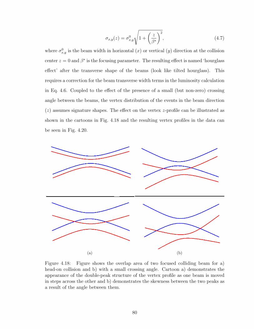
σx,y(z) = σ0x,y
√1 +
(z
β∗
)2
, (4.7)
where σ0x,y is the beam width in horizontal (x) or vertical (y) direction at the collision
center z = 0 and β∗ is the focusing parameter. The resulting effect is named ‘hourglass
effect’ after the transverse shape of the beams (look like tilted hourglass). This
requires a correction for the beam transverse width terms in the luminosity calculation
in Eq. 4.6. Coupled to the effect of the presence of a small (but non-zero) crossing
angle between the beams, the vertex distribution of the events in the beam direction
(z) assumes signature shapes. The effect on the vertex z-profile can be illustrated as
shown in the cartoons in Fig. 4.18 and the resulting vertex profiles in the data can
be seen in Fig. 4.20.
(a) (b)
Figure 4.18: Figure shows the overlap area of two focused colliding beam for a)head-on collision and b) with a small crossing angle. Cartoon a) demonstrates theappearance of the double-peak structure of the vertex profile as one beam is movedin steps across the other and b) demonstrates the skewness between the two peaks asa result of the angle between them.
80
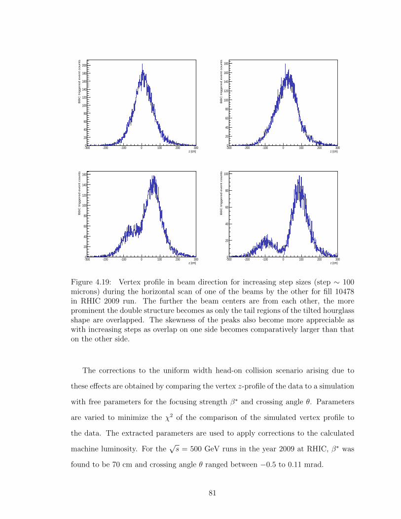
z (cm)-300 -200 -100 0 100 200 300
BB
C triggere
d e
vent counts
0
20
40
60
80
100
120
140
160
180
200
z (cm)-300 -200 -100 0 100 200 300
BB
C triggere
d e
vent counts
0
20
40
60
80
100
120
140
160
180
z (cm)-300 -200 -100 0 100 200 300
BB
C triggere
d e
vent counts
0
20
40
60
80
100
120
140
160
z (cm)-300 -200 -100 0 100 200 300
BB
C triggere
d e
vent counts
0
20
40
60
80
100
Figure 4.19: Vertex profile in beam direction for increasing step sizes (step ∼ 100microns) during the horizontal scan of one of the beams by the other for fill 10478in RHIC 2009 run. The further the beam centers are from each other, the moreprominent the double structure becomes as only the tail regions of the tilted hourglassshape are overlapped. The skewness of the peaks also become more appreciable aswith increasing steps as overlap on one side becomes comparatively larger than thaton the other side.
The corrections to the uniform width head-on collision scenario arising due to
these effects are obtained by comparing the vertex z-profile of the data to a simulation
with free parameters for the focusing strength β∗ and crossing angle θ. Parameters
are varied to minimize the χ2 of the comparison of the simulated vertex profile to
the data. The extracted parameters are used to apply corrections to the calculated
machine luminosity. For the√s = 500 GeV runs in the year 2009 at RHIC, β∗ was
found to be 70 cm and crossing angle θ ranged between −0.5 to 0.11 mrad.
81

z (cm)-300 -200 -100 0 100 200 300
BB
C t
rig
gere
d e
ven
t co
un
ts
0
50
100
150
200
250
300
350
z (cm)-300 -200 -100 0 100 200 300
BB
C t
rig
gere
d e
ven
t co
un
ts
0
50
100
150
200
250
300
350
400
z (cm)-300 -200 -100 0 100 200 300
BB
C t
rig
gere
d e
ven
t co
un
ts
0
50
100
150
200
250
300
350
z (cm)-300 -200 -100 0 100 200 300
BB
C t
rig
gere
d e
ven
t co
un
ts
0
20
40
60
80
100
120
140
160
180
Figure 4.20: Comparison of the vertex profile in beam direction for increasing stepsizes for one side of the vertical scans e.g. (1)top-left : step = 0, (2) top-right : step= 200 microns, (3) bottom-left : step = 350 microns, (4) bottom-right : step = 500microns. In the simulation, β∗ = 70 cm and θ = 0.06 mrad. (Color online) Blackpoints with error bars represent data and open red circles represent simulation.
The sample plots of the measurements shown here are for the√s = 500 GeV p+p
data from the RHIC run in 2009. After applying all the appropriate corrections, the
σBBC was determined to be 32.51 ± 3.01 sys ± 1.19 stat mb. The results were used
to in the measurement of the W boson cross-section from the same data [18]. Using
similar techniques the σBBC for the data (p + p at√s = 62.4 GeV) relevant to the
measurements described here were first measured and used for the neutral pion cross
section measurements [15] and was determined to be 13.7± 1.5 sys mb.
82

4.2.2 Cross Section Results
The cross sections of inclusive charged hadron production in unpolarized p + p
collisions at center of mass energy of 62.4 GeV were calculated and compared to the
theoretical calculations of next-to-leading order accuracy using perturbative QCD.
The measured cross sections results are presented in Figures 5.1 and 5.2. The upper
panel compares our measurement with the NLO calculation with and without the
logarithmic corrections at scale µ = pT . As we will discuss, the next-to-leading
logarithmic corrections have been predicted [62] to be significant for lower energy
systems and previous measurements [15] have indicated that it might be true for low
energy collisions at RHIC. The lower panels show the dependence of the theoretical
calculations on the choice of factorization and renormalization scales for both NLO
and NLL calculations.
4.2.3 Uncertainties on Cross Sections
The largest contribution (11− 24%) to the pT dependent systematic uncertainty
comes from the correction for the detector acceptance and efficiencies. The uncer-
tainty on the cross section due to this correction factor is determined by varying
the selection parameters (selection window in matching variables) in the MC simu-
lations. Another prominent contribution to the systematic uncertainties comes from
the luminosity normalization factor σBBC which is determined with an 11% system-
atic uncertainty. The trigger bias introduces a 2.5% uncertainty. Determination of
the background fraction and the production fraction of separate hadron species each
introduces 1 − 5% pT -dependent systematic uncertainty. Uncertainties from other
sources (e.g. correction for momentum resolution, correction for active area of detec-
tor in experiment and Monte Carlo) are ∼ 1− 2%.
Tables for cross sections and asymmetries are presented below as a function of the
transverse momentum of the produced final state hadrons.
83

Source Systematic UncertaintyσBBC 11%
Trigger bias 2.5%Acceptance & efficiency correction 11-24%
MonteCarlo/data scale factor 2%PID fraction 1-5%
Background fraction 1-5%Momentum smearing correction 1-2%
Table 4.4: Systematic uncertainties of cross section measurements from varioussources.
Mean pT Positive Hadron (h+)(GeV/c) mb GeV−2c2
0.548 (780± 0.12± 110)× 10−2
0.647 (478± 0.0087± 59)× 10−2
0.747 (287± 0.0063± 35)× 10−2
0.847 (173± 0.0046± 21)× 10−2
0.947 (106± 0.0034± 13)× 10−2
1.047 (65.5± 0.025± 8.2)× 10−2
1.147 (41.8± 0.019± 5.2)× 10−2
1.247 (26.7± 0.015± 3.4)× 10−2
1.347 (17.3± 0.012± 2.2)× 10−2
1.447 (11.4± 0.009± 1.4)× 10−2
1.547 (77.3± 0.072± 9.3)× 10−3
1.647 (52.5± 0.057± 6.4)× 10−3
1.747 (35.9± 0.046± 4.4)× 10−3
1.848 (24.6± 0.037± 3.1)× 10−3
1.948 (17.4± 0.030± 2.0)× 10−3
2.110 (9.61± 0.014± 1.1)× 10−3
2.359 (41.9± 0.085± 5.0)× 10−4
2.612 (18.9± 0.055± 2.4)× 10−4
2.861 (8.80± 0.036± 1.2)× 10−4
3.113 (43.3± 0.24± 5.4)× 10−5
3.365 (22.0± 0.16± 2.9)× 10−5
3.616 (10.9± 0.11± 1.7)× 10−5
3.866 (60.3± 0.81± 9.0)× 10−6
4.218 (24.6± 0.35± 6.0)× 10−6
Table 4.5: The cross sections of mid-rapidity charged hadron production from p + pat√s = 62.4 GeV as a function of pT are tabulated along with the corresponding
statistical (second column) and systematic (third column) uncertainties. Cross sec-tions and errors for positive hadrons with the feed-down correction for protons andantiprotons applied (normalization uncertainty of 11.2% not included).
84

Mean pT Negative Hadron (h−)(GeV/c) mb GeV−2c2
0.548 (687± 0.11± 9.3)× 10−2
0.647 (410± 0.080± 5.0)× 10−2
0.747 (245± 0.057± 2.9)× 10−2
0.847 (146± 0.042± 1.7)× 10−2
0.947 (8.83± 0.031± 1.1)× 10−2
1.047 (54.3± 0.023± 6.6)× 10−2
1.147 (34.0± 0.017± 4.1)× 10−2
1.247 (21.6± 0.013± 2.6)× 10−2
1.347 (14.1± 0.010± 1.6)× 10−2
1.447 (9.21± 0.080± 1.1)× 10−2
1.547 (61.1± 0.063± 7.2)× 10−3
1.647 (41.1± 0.050± 4.7)× 10−3
1.747 (27.9± 0.040± 3.3)× 10−3
1.848 (19.0± 0.032± 2.2)× 10−3
1.948 (13.1± 0.026± 1.5)× 10−3
2.110 (73.2± 0.12± 8.3)× 10−4
2.359 (31.4± 0.073± 3.5)× 10−4
2.612 (13.8± 0.046± 1.6)× 10−4
2.861 (63.6± 0.30± 7.5)× 10−5
3.113 (31.2± 0.20± 3.8)× 10−5
3.365 (16.7± 0.14± 2.5)× 10−5
3.616 (7.41± 0.091± 1.1)× 10−5
3.866 (40.2± 0.64± 5.5)× 10−6
4.218 (18.8± 0.29± 5.3)× 10−6
Table 4.6: The cross sections of mid-rapidity charged hadron production from (p+ pat√s = 62.4 GeV as a function of pT are tabulated along with the corresponding
statistical (second column) and systematic (third column) uncertainties. Cross sec-tions and errors for negative hadrons with the feed-down correction for protons andantiprotons applied (normalization uncertainty of 11.2% not included).
85

CHAPTER 5
DISCUSSION OF CROSS SECTION RESULTS
In the overlapping pT range, the cross section results were found to be consistent
with the species-combined cross sections from identified results [15] at PHENIX as
well as identified cross sections at ISR [40] from data at collision energy of√s = 63
GeV. On the upper panels of Figs. 5.1 and 5.2 the cross sections are compared to
the NLO and NLL calculations at a factorization, renormalization and fragmentation
scale of µ = pT [63]. The calculations were performed using MRST2002 unpolarized
PDFs [81] and DSS fragmentation functions [57].
The NLO predictions have been shown to describe cross section results for neutral
pions [24, 13] and charged hadrons [25] at√s = 200 GeV within ∼ 20% for a scale
choice of µ = pT . For the present results at√s = 62.4 GeV, however, the NLO cal-
culations underpredict the data by as much as ∼ 80 % in the case of positive hadrons
and ∼ 60% in the case of negative hadrons for a scale choice of pT . Resummation
of higher order logarithmic terms tend to imrove the pQCD results although these
calculations over predict the data. The lower two panels in the plots show the depen-
dence of the theoretical calculations on the choice of factorization, renormalization
and fragmentation scale (µ) for three different values (pT ,pT2, 2pT ). The inclusion
of higher order terms in the NLL calculations leads to a considerably smaller scale
dependence.
86
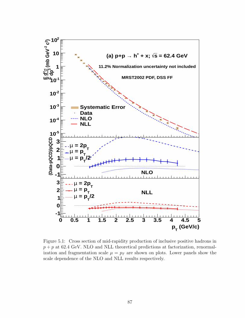
0 0.5 1 1.5 2 2.5 3 3.5 4 4.5 5
)2 c
-2 (m
b G
eV3
dpσ3 d cE
-510
-410
-310
-210
-110
1
10
210
Systematic ErrorDataNLONLL
= 62.4 GeVs + x; + h→(a) p+p
11.2% Normalization uncertainty not included
MRST2002 PDF, DSS FF
0 0.5 1 1.5 2 2.5 3 3.5 4 4.5 5
(Dat
a-pQ
CD
)/pQ
CD
-10123
T = 2pµ
T = pµ
/2T
= pµ
NLO
(GeV/c)T
p0 0.5 1 1.5 2 2.5 3 3.5 4 4.5 5
-1
01
2
3T
= 2pµ
T = pµ
/2T
= pµNLL
Figure 5.1: Cross section of mid-rapidity production of inclusive positive hadrons inp+ p at 62.4 GeV. NLO and NLL theoretical predictions at factorization, renormal-ization and fragmentation scale µ = pT are shown on plots. Lower panels show thescale dependence of the NLO and NLL results respectively.
87

0 0.5 1 1.5 2 2.5 3 3.5 4 4.5 5
)2 c
-2 (m
b G
eV3
dpσ3 d cE
-510
-410
-310
-210
-110
1
10
210
Systematic ErrorDataNLONLL
= 62.4 GeVs + x; - h→(b) p+p
11.2% Normalization uncertainty not included
MRST2002 PDF, DSS FF
0 0.5 1 1.5 2 2.5 3 3.5 4 4.5 5
(Dat
a-pQ
CD
)/pQ
CD
-1
0
1
2
3T
= 2pµT
= pµ/2
T = pµ
NLO
(GeV/c)T
p0 0.5 1 1.5 2 2.5 3 3.5 4 4.5 5
-1
01
2
3T
= 2pµ
T = pµ
/2T
= pµNLL
Figure 5.2: Cross section of mid-rapidity production of inclusive negative hadrons inp+ p at 62.4 GeV. NLO and NLL theoretical predictions at factorization, renormal-ization and fragmentation scale µ = pT are shown on plots. Lower panels show thescale dependence of the NLO and NLL results respectively.
88

These new data at an energy intermediate to typical fixed-target and collider
energies are timely, as the details of how to work with resummation techniques in
different kinematic regimes are currently being explored by the theoretical community
(see for example [62, 61, 39]). Comparison of the present results to the calculations at
NLO with and without NLL terms included indicates that in the measured kinematic
range, NLL terms make relevant contributions to the cross section. However, the
tendency of the NLL calculations to over predict the data, as much as ∼ 40% in
the case of positive hadrons and ∼ 50% in the case of negative hadrons for a scale
choice of pT , may indicate that there are terms in the full NNLO expansion that are
of comparable magnitude and opposite sign to those in the NLL calculation. Possible
inclusion of higer order terms in any future pQCD calculation might describe the data
more closely.
These measurements corroborate similar indications from the neutral pion cross
section results [15] and identified hadron cross section results [20] at PHENIX mea-
sured from data at the same energy. The present measurements can also be useful in a
future determination of inclusive charged hadron fragmentation functions, as progress
in pQCD has allowed inclusion of p+p cross section measurements and semi-inclusive
deep-inelastic lepton-nucleon scattering data in FF parameterizations along with the
traditionally used e+e− data since 2007 [58, 57, 30].
89
CHAPTER 6
DOUBLE HELICITY ASYMMETRY MEASUREMENT
Hadron production in p+ p scattering at√s = 62.4 GeV with transverse momen-
tum pT below 5 GeV/c is mostly dominated by quark-gluon scattering at leading order
in perturbative QCD (pQCD), providing sensitivity to the gluon helicity distribution
in the proton. In the rapidity range (−0.35 < η < 0.35) covered by the PHENIX
central arm detectors [21], scattering of quarks and gluons with momentum fractions
0.05 <∼ xgluon <∼ 0.2 are probed. The double helicity asymmetry ALL is a quantity that
contains information of the parton distributions in the colliding protons. Our present
measurement of ALL of inclusive hadron production in polarized p + p collisions is
sensitive to gluon distribution in leading order.
6.1 Measurement and Correction
6.1.1 Double Helicity Asymmetry and Uncertainty
The measured ALL here is defined as the relative difference between the production
cross sections from collisions of same and opposite helicity protons :
ALL =σ++ − σ+−
σ++ + σ+− (6.1)
where σ++(σ+−) is the production cross section of the species from collisions of same
(opposite) helicity protons. In practice, the polarization of colliding proton beams
90

are not 100%. So, the calculation are normalized by the product of the beam polar-
izations. In terms of measurable quantities, the double helicity asymmetry is :
ALL =1
P1P2
(N++/L++ −N+−/L+−
N++/L++ +N+−/L+−
)(6.2)
=1
P1P2
(N++ −RN+−
N++ +RN+−
)(6.3)
where P1, P2 are the polarizations of two colliding beams, N++(N+−) are hadron track
counts (yields) for same (opposite) helicity configuration of colliding proton bunches
and R = L++/L+− is the relative luminosity of the colliding beams.
PHENIX uses two different luminosity monitors, BBC and ZDC. For luminosity
measurements to be used in the asymmetry measurements, the detector needs to have
high statistics with fairly low backgrounds and it needs to cover the offline vertex
range |zvtx| ≤ 30 cm used for the asymmetry measurements. The vertex restriction is
imposed for essentially two reasons. Firstly, the vertex distribution of the event rate is
almost unchanged within 30 cm region as the complete distribution is fairly Gaussian
with ∼ 60 cm width. Secondly, the iron yoke of the PHENIX central magnet starts
at z = ±40 cm and blocks the particles reaching central arm detectors outside the
selected range. Triggered events at BBC is ∼ 40 times higher than those trigged by
ZDC (a coincidence of hits on both sides of the detector triggers an event). The spatial
resolution of BBC (∼ 5 cm) is much better than that of the ZDC (∼ 30 cm). So the
vertex requirements is more precise while using the BBC as the luminosity monitor.
BBC is therefore used as the luminosity counter for the asymmetry measurements
as it has (a) small background, (b) higher statistical precision and (c) more precise
measurement of z-vertex range.
BBC triggered (‘BBCLL1’ or ‘BBC local level 1’) event counts are recorded for
each bunch crossing and are called ‘scalers’. The relative luminosity R is calculated
fill by fill by adding the scalers corresponding to the same and the opposite helicity
91

bunch crossing separately and taking a ratio of the luminosity for the same to that of
the opposite helicity crossings. Due to the limitation of the bandwidths for the data
acquisition systems and the physics requirements of taking data for several different
trigger settings, only fractions of the triggered events are recorded at PHENIX (typical
in similar collider experiments, a marked difference from the statistically starved
experiments, e.g. neutrino experiments). While calculating relative luminosities for
each fill, the luminosity counts from the BBC scalers were weighted by the pre-scale
factor for the corresponding trigger in each of the runs. Luminosities of BBC and ZDC
triggered events (combined triggers as well as mutually exclusive) were compared to
determine the systematic uncertainty of the relative luminosity measurements. The
method is well described in [48]. The systematic uncertainty of the relative luminosity
measurement was found to be δALL = 1.4× 10⁻³.
The polarization of the two colliding proton beams were obtained from fill by
fill measurements of pC polarimeter results, normalized by the H-jet results [2]. For
the entire data set with the longitudinal beam polarizations, the values for the two
colliding beams (termed ‘Blue’ and ‘yellow’) were 〈PB〉 = 0.481 ± 0.009 (stat) ±
0.032 (sysB) ± 0.014 (sysG) and 〈PY 〉 = 0.479 ± 0.0059 (stat) ± 0.03 (sysB) ±
0.04 (sysG). Final systematic uncertainty on the product of the polarizations 〈PBPY 〉
was found to be ±13.9%.
Since the double helicity asymmetry is a ratio of the cross sections, most of the
systematic uncertainties cancel, rendering the statistical uncertainties of the mea-
surements the relevant ones. The statistical uncertainties of the asymmetries can be
estimated as:
δALL =1
PBPY
2RN++N+−
(N++ +N+−)2
√(∆N++
N++)2 + (
∆N+−
N+− )2, (6.4)
where ∆Ns are the statistical uncertainty in measuring the number of final products
of our interest. For a completely Poissonian distribution(each event contributing
92

maximum of 1 track per bin ), ∆N =√N . However, it is also probable that some
collision events produce more than 1 tracks. So we correct for the ‘enhancement
factor’ coming from the multiplicity distribution to estimate the correct statistical
uncertainties ∆N++ and ∆N+−.
6.1.2 Multiplicity Correction
We look into the multiplicity distribution of positive and negative particle tracks
separately for each of our pT bins Fig. 6.1. With the correction of the enhance-
ment factor, the uncertainty is estimated as ∆N =√
k2
kN , where k is the average
multiplicity. Enhancement factors for different pT bins are listed in the table (6.1).
pT bin(GeV/c) k-factor for (+)ve Hadron k-factor for (-)ve Hadron0.5-1.0 1.022 1.0181.0-2.0 1.007 1.0062.0-3.0 1.001 1.0013.0-4.5 1.0 1.0
Table 6.1: Enhancement factors from multiplicity correction
We measured N++(N+−) from collision data. We measured relative luminosity
using event counts from luminosity monitor BBC. Polarizations were measured by
pC and H-jet polarimeters. For 62.4 GeV data from 2006 run at RHIC, polarization
of each beam was ∼ 58%. All these information were combined to calculate ALL for
each ‘Fill’ at RHIC and then combined statistically to extract the final double helicity
asymmetry result. The background subtracted asymmetry and statistical uncertainty
were calculated as :
ALL =ASig+BGLL − r × ABGLL
1− r(6.5)
δASigLL =
√(δASig+BGLL )2 + r2(ABGLL )2
1− r(6.6)
93

track multiplicity1 2 3 4 5 6 7 8 9 10
co
un
ts
210
310
410
510
610
track multiplicity+h
< 1.0 GeV/cT
0.5 < p
(a)
track multiplicity1 2 3 4 5 6 7 8 9 10
co
un
ts
10
210
310
410
510
610
track multiplicity+h
< 2.0 GeV/cT
1.0 < p
(b)
track multiplicity1 2 3 4 5 6 7 8 9 10
co
un
ts
10
210
310
410
track multiplicity+h
< 3.0 GeV/cT
2.0 < p
(c)
track multiplicity1 2 3 4 5 6 7 8 9 10
co
un
ts
10
210
310
track multiplicity+h
< 4.5 GeV/cT
3.0 < p
(d)
Figure 6.1: Multiplicity distributions of positive hadrons in the transverse momentumbins.
6.1.3 Asymmetry Results
The double helicity asymmetry ALL of the mid-rapidity production of inclusive
hadrons for both charges are presented in the Table. 6.2. The results are plotted along
with pQCD calculations using several different parameterizations of the polarized
PDFs later in Sect. 7 and significance of the results are discussed in detail. However,
several cross checks are also performed to ensure that certain systematics do not
94

contribute as false asymmetries. Two important cross checks (a) measurements of
longitudinal single spin asymmetry (AL) and (b) bunch shuffled measurements of
ALL are discussed respectively in the following Sect. 6.2.1 and Sect. 6.2.2.
pT (GeV/c) ALL ± δALL feed-down ALL ± δALL feed-down(h+) fraction fh+ (h−) fraction fh−
0.68 0.0023± 0.0022 0.022 −0.0065± 0.0024 0.0211.26 −0.01096± 0.0048 0.016 −0.0096± 0.0052 0.0252.29 0.0132± 0.0204 0.012 0.0208± 0.0236 0.0213.40 −0.0299± 0.0517 0.011 −0.0761± 0.0578 0.018
Table 6.2: The double helicity asymmetries and the statistical uncertainties arepresented as a function of pT for positive and negative non-identified charged hadrons.The fractional contribution to the yields from weak-decay feed-down to protons andantiprotons is shown; no correction to the asymmetries has been made for thesecontributions.
6.2 Cross Checks
6.2.1 Single Spin Asymmetries
As we know, the strong force is a parity conserving force. Therefore, parity vi-
olating asymmetry are not expected to be observed. For processed involving hard
scattering (QCD interactions), we do not expect to observe the parity violating lon-
gitudinal single spin asymmetry, defined by :
AL =σ+ − σ−σ+ + σ−
(6.7)
= − 1
P
(N+ −RN−
N+ +RN−
), (6.8)
where σ+, σ− are the cross sections of positive and negative helicity bunches for a
chosen beam (summed over the polarizations of the other beam), N+, N− are the
particle yields for the positive and negative helicity of the chosen beam and P is
the polarization of the said beam. Under parity operator, the momentum vector
95

changes changes sign, whereas the spin does not, resulting in a change of sign in
helicity (which is the dot product of the spin and the momentum). After parity
operation, the longitudinal single spin asymmetry AL as defined above changes sign
too, rendering it to have the only possible zero value.
We measured single spin asymmetries for the ‘blue’ and ‘yellow’ beam separately
for each of the charges and the results were found to be consistent with zero tak-
ing into consideration the statistical uncertainties on the asymmetry measurements.
Figures 6.2 and 6.3 show the results below.
(GeV/c)T
p0 0.5 1 1.5 2 2.5 3 3.5 4 4.5 5
LA
-0.06
-0.05
-0.04
-0.03
-0.02
-0.01
0
0.01
0.02
):Blue Beam+ (hLA
+X+ h→p+p
= 62.4 GeVs
13.9% polarization uncertainty not included±
(a) h+
(GeV/c)T
p0 0.5 1 1.5 2 2.5 3 3.5 4 4.5 5
LA
-0.06
-0.05
-0.04
-0.03
-0.02
-0.01
0
0.01
0.02
):Blue Beam+ (hLA
+X+ h→p+p
= 62.4 GeVs
13.9% polarization uncertainty not included±
(b) h−
Figure 6.2: Single spin asymmetries for the ‘blue’ beam for a) positive and b) negativehadrons.
96
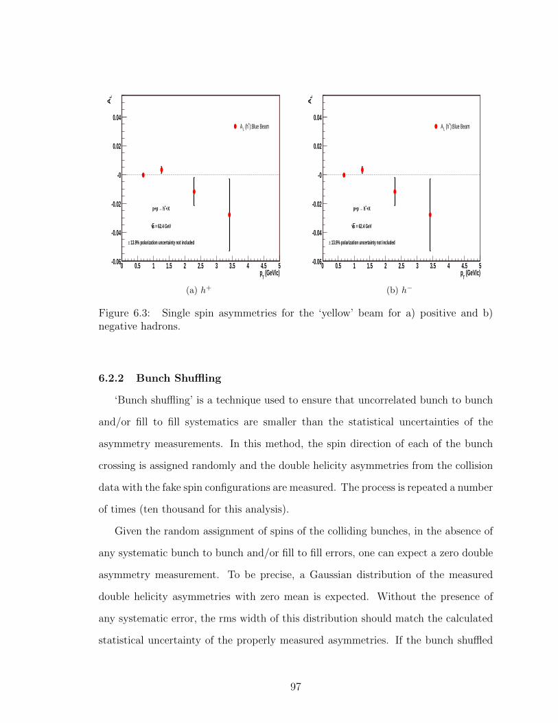
(GeV/c)T
p0 0.5 1 1.5 2 2.5 3 3.5 4 4.5 5
LA
-0.06
-0.04
-0.02
-0
0.02
0.04):Blue Beam+ (hLA
+X+ h→p+p
= 62.4 GeVs
13.9% polarization uncertainty not included±
(a) h+
(GeV/c)T
p0 0.5 1 1.5 2 2.5 3 3.5 4 4.5 5
LA
-0.06
-0.04
-0.02
-0
0.02
0.04):Blue Beam+ (hLA
+X+ h→p+p
= 62.4 GeVs
13.9% polarization uncertainty not included±
(b) h−
Figure 6.3: Single spin asymmetries for the ‘yellow’ beam for a) positive and b)negative hadrons.
6.2.2 Bunch Shuffling
‘Bunch shuffling’ is a technique used to ensure that uncorrelated bunch to bunch
and/or fill to fill systematics are smaller than the statistical uncertainties of the
asymmetry measurements. In this method, the spin direction of each of the bunch
crossing is assigned randomly and the double helicity asymmetries from the collision
data with the fake spin configurations are measured. The process is repeated a number
of times (ten thousand for this analysis).
Given the random assignment of spins of the colliding bunches, in the absence of
any systematic bunch to bunch and/or fill to fill errors, one can expect a zero double
asymmetry measurement. To be precise, a Gaussian distribution of the measured
double helicity asymmetries with zero mean is expected. Without the presence of
any systematic error, the rms width of this distribution should match the calculated
statistical uncertainty of the properly measured asymmetries. If the bunch shuffled
97

distribution shows larger width than the measured statistical uncertainties, it will
indicate the presence of bunch to bunch systematic effects. A detailed study of the
bunch shuffling technique can be found in [31].
Results of the bunched shuffled asymmetry distributions for the positive hadrons
in four pT bins are shown below in Fig. 6.4. The widths of the distributions are
in good agreement with the measured statistical uncertainties of the double helicity
asymmetries as can be seen in the Table. 6.3. The comparison indicates that the ALL
measurements are not affected by bunch to bunch uncorrelated systematic effects.
pT bin δAh+
LL RMS of shuffled δAh−LL RMS of shuffled
(GeV/c) (S+Bkg) Ah+
LL (S+Bkg) Ah−LL
0.5 - 1.0 0.0022 0.0022 0.0023 0.00251.0 - 2.0 0.0046 0.0046 0.0051 0.00492.0 - 3.0 0.020 0.018 0.023 0.0223.0 - 4.5 0.047 0.046 0.051 0.051
Table 6.3: Table for the comparison of statistical uncertainties of double helicityasymmetry measurements and the rms width of the distribution of bunch shuffledfake asymmetries.
98
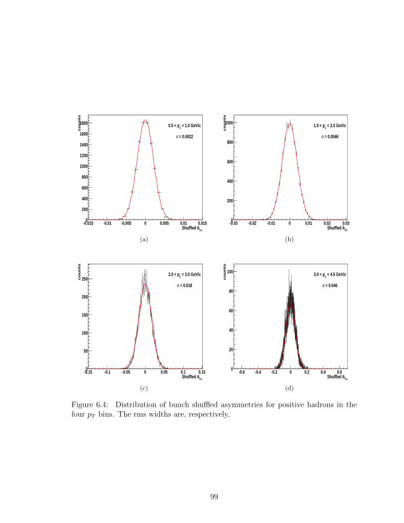
LLShuffled A-0.015 -0.01 -0.005 0 0.005 0.01 0.015
co
un
ts
0
200
400
600
800
1000
1200
1400
1600
1800 < 1.0 GeV/cT
0.5 < p
= 0.0022σ
(a)
LLShuffled A-0.03 -0.02 -0.01 0 0.01 0.02 0.03
co
un
ts0
200
400
600
800
1000 < 2.0 GeV/cT
1.0 < p
= 0.0046σ
(b)
LLShuffled A-0.15 -0.1 -0.05 0 0.05 0.1 0.15
co
un
ts
0
50
100
150
200
250 < 3.0 GeV/c
T2.0 < p
= 0.018σ
(c)
LLShuffled A-0.6 -0.4 -0.2 0 0.2 0.4 0.6
co
un
ts
0
20
40
60
80
100 < 4.5 GeV/cT
3.0 < p
= 0.046σ
(d)
Figure 6.4: Distribution of bunch shuffled asymmetries for positive hadrons in thefour pT bins. The rms widths are, respectively,
99

CHAPTER 7
DISCUSSION OF ASYMMETRY RESULTS
The measured double helicity asymmetries for inclusive charged hadron produc-
tion at mid-rapidity in polarized p + p collisions at√s = 62.4 GeV are presented as
a function of transverse momentum pT in Fig. 7.1 (positive) and Fig. 7.2 (negative).
The asymmetries (Table. 6.2) are compared to NLO pQCD predictions [94] based on
several different parameterizations of polarized PDFs at scale µ = pT .
In the figures the curves labelled “DSSV” refer to deFlorian-Sassot-Stratmann-
Vogelsang (DSSV) parameterizations of the helicity PDFs [59]. Similarly “GRSV”
refer to Gluck-Reya-Stratmann-Vogelsang parameterizations of helicity PDFs [70] and
“BB” refer to Blumlein-Bottcher (BB) parameterizations of the helicity PDFs [47].
DSS fragmentation functions [58] were used for all the calculations. For the calculation
of GRSV and BB curves coordinated-theoretical-experimental-project-on-QCD-6 [86]
unpolarized PDFs were used and MRST2002 [81] unpolarized PDFs were used for the
calculation of DSSV curves. The choice of a different set of unpolarized PDFs was
inspired by the fact that the DSSV polarized PDF sets are based on it and variation
of the calculated quantities due to choice of different unpolarized PDFs were found
to be within current uncertainties.
Polarized DIS data [70, 47, 59] are used to extract parameters of the functional
forms of the PDFs. Figures 7.1 and 7.2 show two instances of GRSV parameteriza-
tions based on the input ∆G(x,Q2) value at an initial scale of Q2 = 0.4 GeV2 : (1)
‘Standard’ scenario with the best fit value ∆G = 0.24 and (2) ‘maximally saturated’
scenario with ∆G(x) = G(x). DSSV [59] parameterizations use RHIC data along
100

with the available pDIS data to constrain parameters of the functional forms of the
polarized PDFs. The asymmetries are also compared to the NLL estimations with
the DSSV PDFs [63].
Figure 7.1: ALL of mid-rapidity inclusive positive hadron production in proton-protoncollisions at
√s = 62.4 GeV with next-to-leading order calculations.
101

Figure 7.2: ALL of mid-rapidity inclusive negative hadron production in proton-proton collisions at
√s = 62.4 GeV with next-to-leading order calculations.
For the purpose of comparison with the experimental results, pQCD calculations
were obtained for separate hadron species (pions, kaons and (anti)protons). Since
our detector does not have uniform efficiency for all species, the species-separated
calculations were combined using the particle fraction in the hadron mixture (Figures
3.5, 3.6) and corresponding detector efficiency (Fig. 4.3 and Fig. 4.4). The measured
asymmetries are small and consistent with zero and they probe a range of approxi-
mately 0.05 ≤ xgluon ≤ 0.2 [62] of the interacting gluons. Since our double helicity
measurements are mostly sensitive to the gluon polarization in leading order these
results indicate that within the probed x-range, gluon helicity distribution ∆g(x)
is small. The results are also consistent with the predictions from the several of
102

the recent parameterizations within statistical limitations. The analysis was based
on comparatively small data set (7 days worth of data at RHIC) and therefore has
fairly large statistical limitations. Even with limited statistics there results clearly
corroborate previous PHENIX measurements [15, 14] that disfavor very large gluon
polarization such as GRSV(max) from 2001. Double helicity asymmetry results pre-
sented here can be used to further constrain ∆g(x) distribution in the probed x-range.
It’s important to state that the measurements with different center-of-mass energies
and over a variety of pT range is required to probe gluon helicity distribution ∆g(x)
over a wide range of x. Especially data from high√s collisions can probe ∆g(x) at
lower x values which is essential in understanding the gluon spin contribution to the
spin of the proton as the parameterizations are poorly constrained resulting in large
uncertainties in this x region.
The charged hadron asymmetries can also be useful in determining the sign of
∆G. Polarized up quark distribution is large and positive whereas polarized down-
quark distribution is negative and smaller numerically. Combined with the fact that
up quarks preferentially fragment into positive pions and down quarks preferentially
fragment into negative pions, polarized pp collisions can generate AΠ+
LL ≥ AΠ0
LL ≥ AΠ−LL
for a positive ∆G and an opposite order for negative ∆G. Since charged pions are
the largest contributor in the measured charged hadron composition and quark-gluon
scattering are the dominant partonic subprocess in the production of most of the final
state particle pT range we measured, present measurements are sensitive to similar
ordering.
103

CHAPTER 8
CONCLUSIONS AND OUTLOOK
8.1 Cross Sections and pQCD
Cross sections at high energy help us to test our understanding of pQCD. Mea-
surements of neutral pion cross sections at PHENIX at various collision energies
(62.4, 200, 500 GeV) and the comparisons of the results (shown in Fig. 8.1) to the
pQCD calculations have demonstrated that next-to-leading order pQCD provides a
very good description of the physics process. As mentioned in the Sect. 1.5, the fixed-
target experiments with√s of tens of GeV indicated that NLO pQCD is inadequate
in the description of the data. Cross section of charged hadrons discussed in this thesis
along with the π0 cross section measurements at PHENIX at the energy of√s = 62.4
GeV have indicated that resummation of next-to-leading logarithmic terms may be
relevant in describing the data at this energy. These measurements are important
contributions towards testing the validity of such techniques and determination of
the range of applicability.
8.2 Longitudinal Spin Program
The understanding of nucleon helicity structure thus fas have mostly been lim-
ited by the availability of high energy data from polarized scattering experiments.
Polarization distributions of quarks and gluons as a function of the momentum frac-
tion are poorly known at both high and very low momentum fraction and the range
of Q2 explored is much narrower than the unpolarized case since the polarized DIS
experiments have been mostly fixed-target. However, the polarized lepton-hadron
104

0 2 4 6 8
-710
-610
-510
-410
-310
-210
-110
1
10
0
2
4
0
2
4
b) NLO
c) NLL
pQCD MRST2002 PDF; fDSS FF
NLL
NLO
a)
µ T = p
)-2
3 (
mb
GeV
c3
/dp
σ3E
d(D
ata
-Q
CD
)/Q
CD
(GeV/c)Tp0 2 4 6 8
(a) 62.4 GeV
0 2 4 6 8 10 12 14 16 18 20
)3
c⋅-2
Ge
V⋅
(m
b3
/dp
σ3E
*d
-910
-810
-710
-610
-510
-410
-310
-210
-110
1
10
210
NLO pQCD(by W.Vogelsang)CTEQ6M PDF; KKP FF
T, 2p
T/2, p
T= pµ
(GeV/c)T
p0 0.5 1 1.5 2 2.5 3 3.5 4 4.5
)3
c⋅-2
Ge
V⋅
(m
b3
/dp
σ3E
*d
-510
-410
-310
-210
-110
1
10
210
0π)/2-π++π(
(GeV/c)T
p0 2 4 6 8 10 12 14 16 18 20
(Da
ta-p
QC
D)/
pQ
CD
-0.5
0
0.5
1 9.7% normalization uncertaintyis not included
(b) 200 GeV (c) 500 GeV
Figure 8.1: Cross sections of mid-rapidity π0 production in proton-proton collisions(a) at
√s = 62.4 GeV [15], (b) at
√s = 200 GeV [13] and (c) at
√s = 500 GeV
(PHENIX preliminary) are compared to next-to-leading order pQCD calculations.
scattering experiments have made it clear that the spins of quarks and anti-quarks
contribute only about 25 − 30% to the nucleon spin. The gluons that carry about
50% of the total momentum distribution of the nucleon, might have been expected
to carry a significant part of the nucleon spin as well, but the knowledge of the gluon
spin distribution have been poor as it can be probed only via scaling violations in
inclusive polarized DIS over limited range of Q2. The spin program at PHENIX and
STAR experiments provided direct access to gluon distributions inside polarized pro-
tons through the polarized p + p collisions. The results have since constrained the
polarized gluon distribution to be small in the probed x range and showed that it is
smaller than various predictions (of ∆G ∼ 1.0 or larger) in the 1990s (Fig. 8.2).
PHENIX experiment has recorded 25 pb−1 of longitudinally polarized p+p data at
√s = 200 GeV over 2005,2006 and 2009 runs at RHIC. The double helicity asymmetry
of neutral pions (Fig. 8.3) have been the flagship measurement for PHENIX over the
105

Figure 8.2: Several predictions for ∆G in the pre-RHIC period![1].
years in order to probe δg(x) as a result of the abundance of neutral pions and the
ability of PHENIX experiment to use high-energy triggers for the events where pi0
decay into two photons. Double helicity asymmetry of π0 production at a lower
collision energy (√s = 62.4 GeV) was measured from 2006 data (Fig. 8.4a).
With increasing luminosity over the years, other probes at PHENIX became
viable. Double helicity asymmetry measurements of η (Fig. 8.5a), direct photon
(Fig. 8.5b) and charged pions (Fig. 8.4b) are shown below. Charged pions, although
as abundant as the neutral pions, are statistically limited due to the lack of a suit-
able trigger. As mentioned before in Sect. 1.5, the charged pion asymmetries are
particularly interesting as the ordering of the asymmetries of the three pion species is
106

(a) separate years (b) combined
Figure 8.3: Neutral pion double helicity asymmetry measurements from p + p at√s = 200 GeV at PHENIX over the years (a) shown separately [1] and (b) combined
(PHENIX preliminary) [1] and compared to calculated asymmetries using DSSV po-larized PDFs.
sensitive to the sign of the ∆G. Direct photon is considered as a clean channel as the
fragmentation is not involved in the process. Eta asymmetry measurement was made
possible using the recent parameterization of η fragmentation with η cross sections
measured at PHENIX along with world e+e− data.
Several different groups of physicists have worked with the existing experimental
data and performed the ‘global analysis’ to extract ∆g(x). The methods and accura-
cies have improved with time as more and more measurements from different channels
and/or probing different Bjorken x-ranges have been made available. As an example,
we show (Fig. 8.6) the NLO estimation of ∆g(x) in 2002 (Stoesslein) and DSSV [59]
result in 2008 which includes RHIC data from both STAR and PHENIX experiments
along with the available polarized DIS data. A quick look at the y-axis promptly
tells the tale of the order of magnitude improvement in narrowing down the uncer-
107

NLONLL
Tp
1 1.5 2 2.5 3 3.5 4
(GeV/c)
-0.04
-0.02
0
0.02
0.04
0.06
0.08
0.1
GRSV-max
G= -G∆
G=0∆
GRSV-std
A
LL
(a) π0 (b) π±
Figure 8.4: Double helicity asymmetry measurements from p+ p at PHENIX for (a)π0 production at
√s = 62.4 GeV [15] and (b) charged pion production at
√s = 200
GeV (PHENIX preliminary) [1].
tainty on such estimations. RHIC data have helped constrain the polarized gluon
distribution δg(x) in the range 0.02 ≤ x ≤ 0.3 and estimated ∆G to be small [59].
However, the uncertainties of the distribution beyond the range is still quite large.
Data from recent years at higher energy of√s = 500 GeV at PHENIX will help to
probe lower x-range and put constraints on δg(x). On the other side of the picture,
asymmetry measurements at the lower energy of 62.4 GeV e.g. charged hadron double
helicity asymmetry discussed in this thesis, will be useful in constraining the δg(x)
distribution in the higher end of x.
At the highest p+p collisions energy of√s = 500 GeV at RHIC, measurements of
cross section and single spin asymmetry of W boson production in the central arms
have been performed. Due to the nature of the weak force, particular charge of the
W boson (mediator of weak force) corresponds to a particular helicity state only.
108
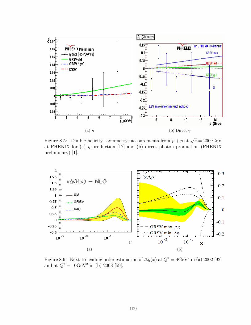
(a) η (b) Direct γ
Figure 8.5: Double helicity asymmetry measurements from p + p at√s = 200 GeV
at PHENIX for (a) η production [17] and (b) direct photon production (PHENIXpreliminary) [1].
(a) (b)
Figure 8.6: Next-to-leading order estimation of ∆g(x) at Q2 = 4GeV2 in (a) 2002 [92]and at Q2 = 10GeV2 in (b) 2008 [59].
109
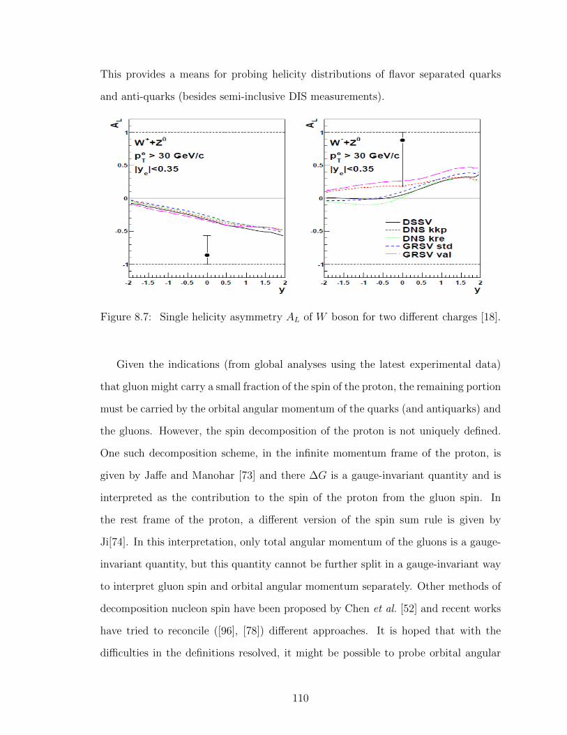
This provides a means for probing helicity distributions of flavor separated quarks
and anti-quarks (besides semi-inclusive DIS measurements).
Figure 8.7: Single helicity asymmetry AL of W boson for two different charges [18].
Given the indications (from global analyses using the latest experimental data)
that gluon might carry a small fraction of the spin of the proton, the remaining portion
must be carried by the orbital angular momentum of the quarks (and antiquarks) and
the gluons. However, the spin decomposition of the proton is not uniquely defined.
One such decomposition scheme, in the infinite momentum frame of the proton, is
given by Jaffe and Manohar [73] and there ∆G is a gauge-invariant quantity and is
interpreted as the contribution to the spin of the proton from the gluon spin. In
the rest frame of the proton, a different version of the spin sum rule is given by
Ji[74]. In this interpretation, only total angular momentum of the gluons is a gauge-
invariant quantity, but this quantity cannot be further split in a gauge-invariant way
to interpret gluon spin and orbital angular momentum separately. Other methods of
decomposition nucleon spin have been proposed by Chen et al. [52] and recent works
have tried to reconcile ([96], [78]) different approaches. It is hoped that with the
difficulties in the definitions resolved, it might be possible to probe orbital angular
110

momentum of quarks and/or gluons to further the understanding of the nucleon
helicity structure.
8.3 Transverse Spin Program
Since early observations of left-right asymmetry AN in high-energy proton scatter-
ing [76], it was indicated that transverse effects play an important role in such scat-
tering experiments. Measurements since then in various other experiments ([9, 8, 36])
have found similar results spurring the interest in the field as all the forward asym-
metries were quite large in contrast to the early expectations based on pQCD. One
possible origin of such large asymmetries could be the transversity distribution de-
scribing the correlation of transversely polarized quarks within a transversely polar-
ized proton analogous to helicity PDF of quarks in longitudinally polarized protons.
This however, is different in a couple of aspects. Firstly, gluons do not have transver-
sity distributions and secondly, it can cannot be probed in QCD processes which are
chiral-even.
The large transverse spin effects observed in semi-inclusive DIS and hadronic col-
lisions have initiated the studies of transverse-momentum-dependent distributions
(TMDs) which are functions of momentum fraction x and Q2 as well as parton trans-
verse momentum kT . The Sivers function [91] is a TMD distribution that describes
the correlation between the intrinsic transverse momentum of the partons within a
transversely polarized nucleon and the direction of the nucleon spin and it can pro-
duce large transverse single spin asymmetries. Measurement of transverse single-spin
asymmetry at PHENIX [26] have been used to put constraints on the gluon sivers
function [80]. Recent measurements at PHENIX [16] of transverse single spin asym-
metry of J/ψ production suggests nonzero tri-gluon correlation functions in trans-
versely polarized protons. In future, single spin asymmetries of charmonium and
111
open heavy flavor production at PHENIX may play important role in understanding
gluon dynamics in the nucleon.
There are also two fragmentation functions that are sensitive to the transversity,
(a) interference fragmentation function [75], which is the collinear FF of two hadrons
from the same scattered parton and (b) the Collins FF [56], which is the correlation
between the transverse spin of a fragmenting quark and its transverse momentum.
Collins FF is therefore transverse-momentum-dependent rather than collinear.
112
BIBLIOGRAPHY
[1] http://www.phenix.bnl.gov/phenix/WWW/docs/decadal/2010/phenix decadal10 full refs.pdf.
[2] http://www4.rcf.bnl.gov/∼cnipol/pubdocs/Run06Offline/NOTE 2006 Polarizations RHIC.txt.
[3] Aaron, F.D., et al. Combined Measurement and QCD Analysis of the Inclusivee+- p Scattering Cross Sections at HERA. JHEP 1001 (2010), 109.
[4] Abe, K., et al. Precision determination of the neutron spin structure fuction gn1 .Phys. Rev. Lett. (July 1997), 26–30.
[5] Abe, K., et al. Measurements of the proton and deuteron spin structure functionsg1 and g2. Phys. Rev. D (October 1998).
[6] Abelev, B. I., et al. Longitudinal double-spin asymmetry and cross section forinclusive jet production in polarized proton collisions at
√s = 200 gev. Phys.
Rev. Lett. 97 (2006).
[7] Abelev, B. I., et al. Longitudinal double-spin asymmetry and cross section forinclusive neutral pion production in polarized proton collisions at
√s = 200 gev.
Phys. Rev. D 80 (2009).
[8] Adams, D. L., et al. Analyzing power in inclusive pi+ and pi- production at highx(f) with a 200-gev polarized proton beam. Phys. Lett. B264 (1991), 462–466.
[9] Adams, D. L., et al. Comparison of spin asymmetries and cross-sections in pi0production by 200-gev polarized anti-protons and protons. Phys. Lett. B261(1991), 201–206.
[10] Adams, J., et al. Cross sections and transverse single-spin asymmetries in forwardneutral-pion production from proton collisions at
√s = 200 gev. Phys. Rev. Lett.
92 (2004).
[11] Adare, A., et al. High-pT charged hadron suppression in Au + Au collisions at√sNN = 200 GeV. Phys. Rev. C 69 (2004), 034910.
[12] Adare, A., et al. Measurement of high-pT single electrons from heavy-flavordecays in p + p collisions at
√s = 200 GeV. Phys. Rev. Lett. 97 (Dec 2006),
252002.
113

[13] Adare, A., et al. Inclusive cross section and double helicity asymmetry for π0
production in p+ p collisions at√
(s) = 200 gev: Implications for the polarizedgluon distribution in the proton. Phys. Rev. D. 76 (2007), 051106(R).
[14] Adare, A., et al. Gluon-spin contribution to the proton spin from the double-helicity asymmetry in inclusive π0 production in polarized p + p collisions at√sNN = 200 gev. Phys. Rev. Lett. 103 (2009), 082002.
[15] Adare, A., et al. Inclusive cross section and double helicity asymmetry for π0
production in p+p collisions at√s = 62.4 gev. Phys. Rev. D 79 (2009), 012003.
[16] Adare, A., et al. Measurement of transverse single-spin asymmetries for j/ψproduction in polarized p+p collisions at
√s = 200 GeV. Phys. Rev. D 82 (Dec
2010), 112008.
[17] Adare, A., et al. Cross section and double helicity asymmetry for η mesons andtheir comparison to π0 production in p + p collisions at
√s = 200 GeV. Phys.
Rev. D 83 (2011), 032001.
[18] Adare, A., et al. Cross section and parity-violating spin asymmetries of W±
boson production in polarized p + p collisions at√s = 500 GeV. Phys. Rev.
Lett. 106 (Feb 2011), 062001.
[19] Adare, A., et al. Event structure and double helicity asymmetry in jet productionfrom polarized p + p collisions at
√s = 200 GeV. Phys. Rev. D 84 (Jul 2011),
012006.
[20] Adare, A., et al. Identified charged hadron spectra in p+ p collisions at√s=200
and 62.4 gev. Phys. Rev. C 83 (2011), 064903.
[21] Adcox, K., et al. Phenix central arm tracking detectors. Nucl. Instr. and Meth.A 499 (March 2003), 489–507.
[22] Adcox, K., et al. Phenix detector overview. Nucl. Instr. and Meth. A 499 (March2003), 469–479.
[23] Adler, S., et al. High-pT charged hadron suppression in Au + Au collisions at√sNN = 200 GeV. Phys. Rev. C 69 (Mar 2004), 034910.
[24] Adler, S. S., et al. Absence of suppression in particle production at large trans-verse momentum in
√s = 200 gev d+ au collisions. Phys. Rev. Lett. 91 (2003),
072303.
[25] Adler, S. S., et al. Measurement of transverse single-spin asymmetries for midra-pidity production of neutral pions and charged hadrons in polarized p + p colli-sions at
√s = 200 gev. Phys. Rev. Lett. 95 (2005).
[26] Adler, S. S., et al. Measurement of transverse single-spin asymmetries for midra-pidity production of neutral pions and charged hadrons in polarized p + p colli-sions at
√s = 200 GeV. Phys. Rev. Lett. 95 (Nov 2005), 202001.
114

[27] Adler, S. S., et al. Measurement of direct photon production in p+p collisionsat√s = 200 gev. Phys. Rev. Lett. 98 (2007), 012002.
[28] Adler, S. S., et al. Modifications to di-jet hadron pair correlations in au + aucollisions at
√(sNN) = 200 gev. Phys. Rev. Lett. 97 (2007), 052301.
[29] Adler, S. S., et al. Centrality dependence of charged hadron in deuteron+goldand nucleon+gold collisions at
√sNN=200 gev. Phys. Rev. C 77 (2008), 014905.
[30] Aidala, Christine A., Ellinghaus, Frank, Sassot, Rodolfo, Seele, Joseph P., andStratmann, Marco. Global analysis of fragmentation functions for eta mesons.Phys. Rev. D 83 (2011), 034002.
[31] Aidala, Christine Angela. Meaurement of the Transverse Single-Spin Asymmetryfor Mid-rapidity Production of Neutral Pions in Polarized p+p Collisions at 200GeV Center-of-Mass Energy. PhD thesis, Columbia University, 2006.
[32] Airapetian, A., et al. Precise determination of the spin structure function g1 ofthe proton, deuteron and neutron. Phys. Rev. D 75 (2007), 012007.
[33] Aizawa, M., et al. Phenix central arm particle id detectors. Nucl. Instr. andMeth. A 499 (2003), 508–520.
[34] Alekseev, I., et al. Polarized proton collider at rhic. Nucl. Instrum. Methods A499 (2003), 392–414.
[35] Alekseev, I. G., et al. Analyzing power in CNI-region at AGS (experiment E950).AIP Conf. Proc. 549 (2000), 670–673.
[36] Alekseev, M., et al. Measurement of the collins and sivers asymmetries on trans-versely polarised protons. Phys. Lett. B692 (2010), 240–246.
[37] Alguard, M. J., et al. Deep inelastic scattering of polarized electrons by polarizedprotons. Phys. Rev. Lett. 37 (Nov 1976), 1261–1265.
[38] Allen, M., et al. Phenix inner detectors. Nucl. Instr. and Meth. A 499 (2003),549–559.
[39] Almeida, Leandro G., Sterman, George F., and Vogelsang, Werner. Thresholdresummation for di-hadron production in hadronic collisions. Phys. Rev. D 80(2009), 074016.
[40] Alper, B., et al. The production of charged particles with high transverse mo-mentum in proton-proton collisions at the cern isr. Nucl. Phys. B 87 (1975).
[41] Altarelli, Guido, and Parisi, G. Asymptotic Freedom in Parton Language. Nucl.Phys. B126 (1977), 298.
[42] Aphecetche, L., et al. Phenix calorimeter. Nucl. Instr. and Meth. A 499 (2003),521–536.
115
[43] Aronson, S.H., et al. Nucl. Instrum. Methods A 499 (2003), 480.
[44] Ashman, J., et al. A measurement of the spin asymmetry and determination ofthe structure function g1 in deep inelastic muon-proton scattering. Phys. Lett.B (May 1988), 364–370.
[45] Bass, Steven D. The spin structure of the proton. Rev. Mod. Phys. 77 (November2005), 1257.
[46] Baum, G., et al. New measurement of deep-inelastic e − p asymmetries. Phys.Rev. Lett. 51 (Sep 1983), 1135–1138.
[47] Blumlein, Johannes, and Bottcher, Helmut. Qcd analysis of polarized deep in-elastic scattering data. Nucl. Phys. B 841 (2010), 205–230.
[48] Boyle, Kieran Peter. Measurements of the Double Helicity Asymmetry in PionProduction in Proton Collisions at
√s = 200 GeV and the Resulting Constraints
on the Polarized Gluon Distribution in the Proton. PhD thesis, Stony BrookUniversity, 2008.
[49] Breidenbach, M., Friedman, J. I., Kendall, H. W., Bloom, E. D., Coward, D. H.,DeStaebler, H., Drees, J., Mo, L. W., and Taylor, R. E. Observed behaviorof highly inelastic electron-proton scattering. Phys. Rev. Lett. 23 (Oct 1969),935–939.
[50] Bunce, G., Saito, N., Soffer, J., and Vogelsang, W. Ann. Rev. Nucl. Part. Sci.50 (2000), 525–575.
[51] CERN Program Library. GEANT 3.2.1, 1993.http://wwwasdoc.web.cern.ch/wwwasdoc/pdfdir/geant.pdf.
[52] Chen, Xiang-Song, Lu, Xiao-Fu, Sun, Wei-Min, Wang, Fan, and Goldman, T.Spin and orbital angular momentum in gauge theories: Nucleon spin structureand multipole radiation revisited. Phys. Rev. Lett. 100 (2008), 232002.
[53] Chodos, A., Jaffe, R. L., JOhnson, K., and Thorn, C. B. Baryon structure inthe bag theory. Phys. Rev. D 9 (1974).
[54] Christy, E. M., et al. Measurements of electron-proton elastic cross sections for0.4 < Q2 < 5.5 (GeVc)2. Phys. Rev. C 70 (Jul 2004), 015206.
[55] Collins, J. C., Soper, D. E., and Sterman, G. Soft gluons and factorization. Nucl.Phys. B 308 (1988), 833.
[56] Collins, John C. Leading twist single transverse-spin asymmetries: Drell-yanand deep inelastic scattering. Phys. Lett. B536 (2002), 43–48.
[57] de Florian, D., Sassot, Rodolfo, and Stratmann, Marco. Global analysis of frag-mentation functions for pions and charged hadrons. Phyis. Rev. D 76 (2007).
116

[58] de Florian, D., Sassot, Rodolfo, and Stratmann, Marco. Global analysis of frag-mentation functions for pions and kaons and their uncertainties. Phys. Rev. D75 (2009), 114010.
[59] de Florian, D., Sassot, Rodolfo, Stratmann, Marco, and Vogelsang, W. Globalanalysis of helicity parton densities and their uncertainties. Phys. Rev. Lett. 101(2008), 072001.
[60] de Florian, D., Sassot, Rodolfo, Stratmann, Marco, and Vogelsang, W. Extrac-tion of spin-dependent parton densities and their uncertainties. Phys. Rev. D 80(2009), 034030.
[61] de Florian, D., and Vogelsang, W. Threshold resummation for the inclusive-hadron cross section in pp collisions. Phys. Rev. D. 71 (2005), 114004.
[62] de Florian, D., Vogelsang, W., and Wagner, F. Single-inclusive hadron produc-tion in polarized pp scattering at next-to-leading logarithmic accuracy. Phys.Rev. D. 76 (2007), 094021.
[63] de Florian, D., and Wagner, F. private communication, 2010.
[64] Drijard, D., et al. NEUTRAL STRANGE PARTICLE PRODUCTION IN PRO-TON PROTON COLLISIONS AT
√s = 63-GeV. Zeit. Phys. C12 (1982), 217.
[65] Ellis, John, and Jaffe, Robert. Sum rule for deep-inelastic electroproduction frompolarized protons. Phys. Rev. D 9, 5 (1974), 1444–1446.
[66] Ellis, R. K., Georgi, H., Machacek, M., Politzer, H. D., and Ross, G. G. Factor-ization and the parton model in qcd. Phys. Lett. B 78 (1978), 281.
[67] Esterman, I., and Stern, O. Uber die magnetische Ablenkung von Wasserstoff-molekulen und das magnetische Moment des Protons. II. Zeitschrift fur Physik85 (Jan. 1933), 17–24.
[68] Feynman, Richard P. Very high-energy collisions of hadrons. Phys. Rev. Lett.23 (1969), 1415–1417.
[69] Frisch, R., and Stern, O. Uber die magnetische Ablenkung von Wasserstoff-molekulen und das magnetische Moment des Protons. I. Zeitschrift fur Physik85 (Jan. 1933), 4–16.
[70] Gluck, M., Reya, E., Stratmann, M., and Vogelsang, W. Models for the polarizedparton distributions of the nucleon. Phys. Rev. D. 63 (2001), 094005.
[71] Graudenz, D., Hampel, M., Vogt, A., and Berger, Christoph. The Mellin trans-form technique for the extraction of the gluon density. Z. Phys. C70 (1996),77–82.
[72] Hughes, E. W., and Voss, R. Spin structure functions. Annu. Rev. Nucl. Part.Sci. (1999), 303–339.
117

[73] Jaffe, Robert L., and Manohar, Aneesh. The g1 problem : Deep inelastic electronscattering of the proton. Nucl. Phys. B 337 (1990), 509–546.
[74] Ji, Xiangdong. Lorentz symmetry and the internal structure of the nucleon.Phys. Rev. D 58 (Jul 1998), 056003.
[75] John C. Collins, Steve F. Heppelmann, and Ladinsky, Glenn A. Measuringtransversity densities in singly polarized hadron-hadron and lepton-hadron col-lisions. Nucl. Phys. B420 (1994), 565–582.
[76] Klem, R., et al. Measurement of Asymmetries of Inclusive Pion Production inProton Proton Interactions at 6 GeV/c and 11.8 GeV/c. Phys. Rev. Lett. (1976),929–931.
[77] Kosower, David A. Extracting parton densities from collider data. Nucl.Phys.B520 (1998), 263–278.
[78] Leader, Elliot. On the controversy concerning the definition of quark and gluonsangular momentum. Phys. Rev. D 83 (2011), 096012.
[79] Leader, Elliot, Sidorov, Aleksander, and Stamenov, Dimiter. Determination ofpolarized parton densities from a QCD analysis of inclusive and semi-inclusivedeep inelastic scattering data. Phys. Rev. D 82 (2010), 114018.
[80] M. Anselmino, U. D’Alesio, S. Melis, and Murgia, F. Constraints on the gluonsivers distribution via transverse single spin asymmetries at mid-rapidity inp↑p→ π0x processes at rhic. Phys. Rev. D 74 (2006), 094011.
[81] Martin, A.D., Roberts, R.G., Stirling, W.J., and Thorne, R.S. Uncertainties ofpredictions from parton distributions. 1: Experimental errors. Eur.Phys.J. C28(2003), 455–473.
[82] Martin, A.D., Stirling, W.J., Thorne, R.S., and Watt, G. Parton distributionsfor the LHC. Eur.Phys.J. C63 (2009), 189–285.
[83] McAllister, R. W., and Hofstadter, R. Elastic scattering of 188-mev electronsfrom the proton and the alpha particle. Phys. Rev. 102 (May 1956), 851–856.
[84] Nakagawa, I., et al. Polarization measurements of rhic-pp run05 using cni pc-polarimeter. AIP Conf. Proc. 915 (June 2007), 912–915.
[85] Okada, H., et al. Measurement of the analyzing power an in pp elastic scatteringin the cni region with a polarized atomic hydrogen gas jet target. Phys. Lett. B638 (2006), 450.
[86] Pumplin, J., Stump, D.R., Huston, J., Lai, H.L., Nadolsky, Pavel M., et al. Newgeneration of parton distributions with uncertainties from global QCD analysis.JHEP 0207 (2002), 012.
118

[87] Punjabi, V., et al. Proton elastic form factor ratios to Q2 = 3.5-GeV2 by polar-ization transfer. Phys. Rev. C71 (2005), 055202.
[88] Qattan, I. A., et al. Precision rosenbluth measurement of the proton elastic formfactors. Phys. Rev. Lett. 94 (2005), 142301.
[89] Rosenbluth, M. N. High energy elastic scattering of electrons on protons. Phys.Rev. 79 (Aug 1950), 615–619.
[90] Roser, T. Acceleration of polarized beams using multiple strong partial snakes.Proceedings of the 16th International Spin SPhysics Symposium (SPIN2004)(2005), 687.
[91] Sivers, Dennis. Single-spin production asymmetries from the hard scattering ofpointlike constituents. Phys. Rev. D 41 (Jan 1990), 83–90.
[92] Stosslein, U. Status and perspectives of spin physics. Acta Phys. Polon. B33(2002), 2813–2834.
[93] Stratmann, Marco, and Vogelsang, Werner. Towards a global analysis of polar-ized parton distributions. Phys.Rev. D64 (2001), 114007.
[94] Taneja, S. private communication, 2010.
[95] Vogelsang, W. private communication, 2008.
[96] Wakamatsu, M. Gauge and frame-independent decomposition of nucleon spin.Phys.Rev. D 83 (2011), 014012.
[97] Walker, R. C., et al. Measurements of the proton elastic form factors for 1 <q2 < 3 gev2 at slac. Phys. Rev. D 49 (Jun 1994), 5671–5689.
[98] Zhan, X., Allada, K., Armstrong, D.S., Arrington, J., Bertozzi, W., et al. HighPrecision Measurement of the Proton Elastic Form Factor Ratio µpGE/GM atlow Q2. Phys.Lett. B705 (2011), 59–64.
119