Under-relaxed Quasi-Newton acceleration for an

inverse fixed-point problem coming from

Positron-Emission Tomography

T. Martini∗† L. Reips‡ J. M. Martınez∗§

June 27, 2016

Abstract

Quasi-Newton acceleration is an interesting tool to improve theperformance of numerical methods based on the fixed-point paradigm.In this work the quasi-Newton technique will be applied to an inverseproblem that comes from Positron Emission Tomography, whose fixed-point counterpart has been introduced recently. It will be shown thatthe improvement caused by the quasi-Newton acceleration procedureis very impressive.

Key words: Positron Emission Tomography, Fixed-point methods,Quasi-Newton acceleration.

1 Introduction

Given a function G : IRn → IRn the fixed-point problem consists of findingx ∈ IRn such that x = G(x). Associated to this problem one can define thenonlinear system of equations

F (x) = 0 (1)

∗Department of Applied Mathematics, IMECC-UNICAMP, University of Campinas,Campinas SP, Brazil.†E-mail: tiaramartini@gmail.com‡Department of Exact Sciences and Education, Federal University of Santa Catarina,

Blumenau SC, Brazil. E-mail: l.reips@ufsc.br§E-mail: martinez@ime.unicamp.br

1

where F : IRn → IRn is defined by F (x) = x−G(x).Quasi-Newton methods solve (1) with less computational effort (per it-

eration) than Newton’s method, without losing most of Newton’s good con-vergence properties. A quasi-Newton iteration can be seen as a genera-lization of the Newtonian iteration, in which one replaces the Jacobian ma-trix F ′(x) by some approximation, which may not involve calculations ofderivatives. Here, we will discuss the use of quasi-Newton methods as ac-celerators of iterative procedures whose rate of convergence is merely linear.Since quasi-Newton methods usually converge superlinearly [28], we hopethat this property will be inherited by the quasi-Newton acceleration offixed-point iterations.

Fixed-point problems arise naturally in electronic structure calculation[21], complex models of transport [5], statistics [42], dynamic PET recon-struction [36, 37] and many other problems. PET reconstruction is the focusof our work. A major concern about the fixed-point iteration xk+1 = G(xk)is the fact that the iterates can converge with linear and extremely slowrate, motivating many acceleration studies [5, 14, 16, 20, 21, 24, 33, 38, 39,41, 43, 44, 47].

Positron Emission Tomography (PET) is an imaging technique appliedin nuclear medicine that produces images of physiological processes in 2D or3D. This procedure has emerged as a research tool to study the brain and,despite its high cost, provides good diagnostic imaging in a minimally inva-sive manner, thus becoming a useful clinical tool. We are interested in theexamination of cardiac myocardial perfusion, although the PET techniqueis also applied in a wide range of procedures,as detection and monitoringactivity of malignant tumors and brain disorders, including early diagnosisof Alzheimer’s disease [32, 34, 36].

For low quality data, for example in tracers like H152 O with low half-life

(fast decay), new approaches based on the direct reconstruction of param-eters from PET data instead of an intermediate image reconstruction stephave evolved as promising tools [2, 3], at least for preclinical investigations.

In this paper we will present our experience with under-relaxed quasi-Newton acceleration techniques for reconstruction of the kinetic behavior ofa radioactive tracer during cardiac perfusion with real PET data. We willshow that significative improvement may be obtained in comparison withthe original fixed-point algorithm.

2

2 Positron Emission Tomography (PET) Model

This section is based on the PhD Thesis of Reips [36], whose main objec-tive was to reconstruct, directly, the kinetic behavior of radioactive water,H15

2 O, based on real data obtained from PET scans during cardiac per-fusion exams. In [36] the parameter identification problem associated withthe inverse problem of image reconstruction was formulated. Its solution ledto recover kinetic parameters associated to a suitable differential equationsmodel.

In order to analyse PET data and estimate metabolic rates, compart-mental models are generally used. These models are able to describe fairlywell a large number of physiological processes within brain and heart. Manymethods have been developed based on compartmental models. Cerebraloxygen processes were considered in [31], neuroreceptor ligand binding in[30], and quantification of blood flow in [1, 3, 4, 26, 25].

In compartmental models, each compartment defines one possible state(for example, physical location and chemical state) of the tracer. A singlecompartment uses to be a group of states [9]. Considering the PET image-sequence, fixed spatial compartments are areas defined by the concentrationof a radioactive tracer (called activity) represented by a temporal function.

The images produced by PET scanners consist of many overlapping sig-nals (measurements of radioactivity levels). Consequently, in order to isolatethe desired component it is necessary to use a mathematical model, whichincludes all possible states (treated as a single compartment [45]) of thesignal given by a PET-reconstruction sequence.

In order to describe the interaction between compartments, one asso-ciates a constant capable to represent the velocity of absorption, i.e. thediffusion of the radioactive trace used by the PET scan. Thus, data con-cerning the rate at which the radioactive tracer is metabolized in the regionof interest can be associated with rates of variation in time of the tracerconcentrations in each compartment [9]. Moreover, the rate of passage ofsubstances between the regions are represented by means of a constant link-ing these compartments.

In this way, it becomes possible to describe the kinetics behavior of aradioactive tracer in a physiological system employing a set of nonlinear dif-ferential equations. The variation of temporal concentration of the radioac-tive tracer is analyzed in a specific compartment and, thus, the quantitiesof interest can be determined.

The three-component reaction-diffusion model of [36] is a macroscopicmodel for cardiovascular perfusion that predicts the tracer activity (a tem-

3

poral function) if the reaction rates, velocities, and diffusion coefficients areknown, based on compartmental models [9, 45]. The three components pre-viously mentioned are denoted by arteries, veins and tissues (capillaries).

Let Ω ⊆ IR3 be a bounded domain representing the region of interest andlet t ∈ [0, T ]. We consider x ∈ Ω as a macroscopic variable homogenizingmicroscopic flow patterns. Thus, for the activity u = u(x, t) we have

u(x, t) = CA(x, t) + CV(x, t) + CT (x, t)

and each concentration C is associated with local velocities VA, VV , VT andlocal diffusion coefficients DA, DV , DT , respectively. Direct reconstructionsof distributed parameters models from PET data can be found in [3, 23].

With the sinogram PET it is possible to formulate the dynamic inverseproblem using a model encoded by an operator G, that maps parameters pto a time evolution of activity u:

℘(Ku(x, t)) = f(x, t), u = G(p), (2)

where f : Ω × IR → IR is a sequence of measured PET data on a domainΩ, ℘(z) denotes a Poisson random variable with expectation z, and K :L2(Ω) → L2(Ω)1 is the forward operator. As going into the details aboutK is beyond the scope of this work, we suggest the book of Wernick [45] forthe interested reader.

Working with inverse problems have a disadvantage as the problem isusually ill-posed in the sens of Hadamard [17]. Thus, regularization methodsare added and the solution of the above inverse problem is given by thefollowing minimization problem

(u, p) ∈ arg min(u,p)

T∫0

∫ΩKu(x, t)− f(x, t)log(Ku(x, t))dx dt+ αR(p) (3)

where R is a regularization functional, which incorporates smoothness anda-priori information about typical values of the parameters. Several meth-ods can be found in the literature applied to the regularization of ill-posedproblems: Gauss-Newton [6], Levenberg-Marquardt methods [18], Landwe-ber methods [19, 35] and Newton-type methods [22].

1We denote by L2(X) the set of Lebesgue measurable functions such that ||f ||L2(X) <

∞, where ||f ||L2(X) =(∫

|f |2dµ) 1

2 .

4

All the biological parameters represented in p are found by solving theminimization problem (3). Moreover, using the differential equations modelproposed in [36] it is possible to predict the flow behavior of the radioactivetracer during the cardiac perfusion PET.

In order to solve (3) for noise free-data, Reips [36], as others in literature[13, 15, 46], used the well-known Expectation Maximization (EM) Algorithm[11]. Thus, given an image uk = G(pk), one computes uk+ 1

2by

uk+ 12

=ukK∗1

K∗(

f

Kuk

), (4)

where 1 denotes the constant function equal one, K∗ is the adjoint operatorof K and uk+ 1

2, uk and f are spatially and temporally dependent of x and

t, respectively.Note that this step is well defined since, as usual for EM, the operations

are performed punctually, i.e., element by element. After solving the associ-ated lagrangean functionals, we calculate all the biologicals parameters thatcomposes the vector p. The second half-step (backward splitting step) isdefined by

pk+1 ∈ arg minp

T∫0

∫Ωωk(x, t)(G(p)(x, t)− uk+ 1

2(x, t))2dx dt+ αR(p), (5)

where ωk = K∗1G(pk)

. The new image uk+1 is updated from the biological

parameters found and the process is restarted.Although the results in [36] indicate that the model provides, with good

accuracy, the activity of the radioactive tracer, the number of fixed pointiterations that are necessary to obtain accurate results is very high, thusleading to unaffordable computational cost. Consequently, accelerating theReaction-Diffusion Model from PET data is mandatory.

3 Quasi-Newton acceleration for PET calculations

For an arbitrary parameter p ∈ IRn let us define p+ = G(p) as the nextiterate that comes from the application of the Forward-Backward Splitting(FBS) [10] scheme to (3). In this way, a fixed-point (FP) iteration is definedas an iteration of the FBS method.

As we mentioned before, solving a fixed-point problem corresponds tosolve a nonlinear system of equations F (p) = 0, where F (p) = p − G(p).

5

However, the Jacobian of F may not be available, or may be extremelydifficut to compute.

In order to choose the most appropriate class of methods to improve theconvergence rate of fixed-point iterates, the intrinsic characteristics of theseproblems must be taken into account. Usually [5, 16] practical fixed-pointproblems are high-dimensional, so it is interesting to use accelerators thatdo not require matrix inversion and that can be implemented using limited-memory techniques. In addition, line search procedures are not recommend-able because the cost of function evaluations may be very high [16]. Thismeans that we should accelerate employinng well established quasi-Newtontechniques that ensure local convergence without line searches.

We will show how to solve the associated nonlinear system F (p) = 0using several quasi-Newton methods that belong to the secant type, becausethe approximate Jacobians satisfy the so called secant equation [28]. Bydefinition, the FBS iteration corresponds to:

pk+1 = pk −H0F (pk)

with H0 = I. Since this iteration converges locally at a linear rate, it isnatural to conjecture that quasi-Newton methods based on

pk+1 = pk −HkF (pk) or pk+1 = pk −B−1k F (pk),

where Hk satisfies the secant equation Hk+1(F (pk+1)− F (pk)) = pk+1 − pk(or alternatively, Bk+1(pk+1 − pk) = F (pk+1) − F (pk)) with some minimalvariation principle, probably converge superlinearly, thus accelerating theconvergence of the FBS method.

In the following subsection we describe the quasi-Newton acceleratorsconsidered in this research.

3.1 Quasi-Newton methods employed in this study

We considered five different matrix updating schemes that satisfy the secant(or the inverse secant) equation, namely: Broyden’s First and Second Meth-ods [7], Column Updating Method [27], Inverse Column Updating Method[29] and Thomas’ Method [40].

We may formulate the updating procedure of these methods by:

Bk+1 = Bk +(yk −Bksk)v>k

s>k vk, (6)

where sk = xk+1 − xk, yk = F (xk+1)− F (xk) and vk ∈ IRn.

6

The choice vk = sk defines Broyden’s First Method (BM1), vk = ek de-

fines the Column Updating Method (COLUM), and vk =

(Pk +

‖sk‖2

I

)sk

corresponds to Thomas’ method, where

Pk+1 = (1 + ‖sk‖)(‖sk‖I + Pk −

wkw>k

w>k sk

), P0 = ρ2I.

Applying the Sherman-Morrison formula to (6) we obtain

B−1k+1 = B−1

k +(sk −B−1

k yk)v>k B−1k

v>k B−1k yk

(7)

or, equivalently,

B−1k+1 = (I + ukv

>k )B−1

k =

k∏i=0

(I + uiv>i )B−1

0 , (8)

where uk =sk −B−1

k yk

v>k B−1k yk

. In order to save some memory storage, we used

the updating trick described in [12], justified by the following lemma.

Lemma 3.1 Let dk = −B−1k F (xk), zk = B−1

k yk, zi = B−1i yk, γi =

s>i zis>i zi

,

and τk =s>k dks>k zk

. Consider xk+1 = xk + αkdk and assume that s>i zi 6= 0,

i = 0, 1, . . . , k − 1. Then,

(i) dk+1 = dk − sk + τk(sk − zk) and

(ii) zi+1 = zi + γiτi

(di+1 − (1− αi)di).

Proof. See Lemma 2.2 of [12].On the other hand, among the methods inspired by the inverse se-

cant equation, we used Broyden’s Second Method (BM2) and the InverseColumn-Updating Method (ICOLUM). For these methods, we have

B−1k+1 = B−1

k +(sk −B−1

k yk)v>k

v>k yk, (9)

where vk = yk for BM2 and vk = ek for ICOLUM.Note that we can write (9) as

B−1k+1 = B−1

k + wkv>k = B−1

0 +

k∑i=0

wiv>i (10)

7

where

wk =sk −B−1

k yk

v>k yk.

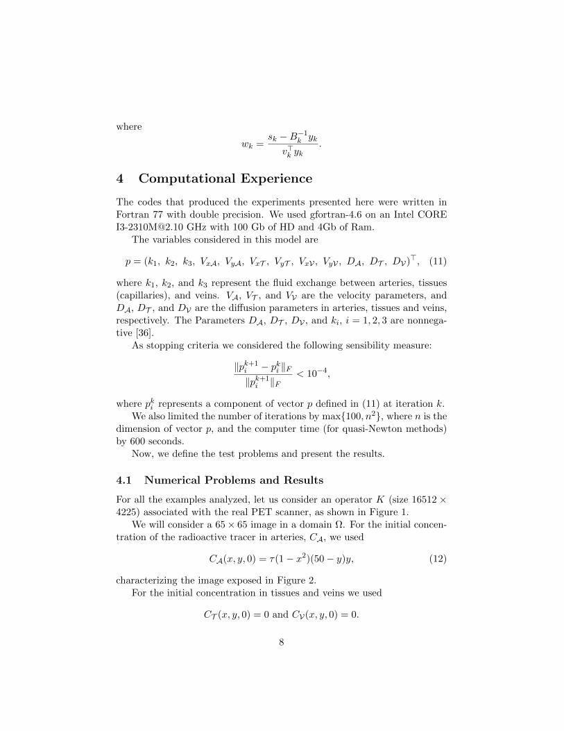
4 Computational Experience

The codes that produced the experiments presented here were written inFortran 77 with double precision. We used gfortran-4.6 on an Intel COREI3-2310M@2.10 GHz with 100 Gb of HD and 4Gb of Ram.

The variables considered in this model are

p = (k1, k2, k3, VxA, VyA, VxT , VyT , VxV , VyV , DA, DT , DV)>, (11)

where k1, k2, and k3 represent the fluid exchange between arteries, tissues(capillaries), and veins. VA, VT , and VV are the velocity parameters, andDA, DT , and DV are the diffusion parameters in arteries, tissues and veins,respectively. The Parameters DA, DT , DV , and ki, i = 1, 2, 3 are nonnega-tive [36].

As stopping criteria we considered the following sensibility measure:

‖pk+1i − pki ‖F‖pk+1i ‖F

< 10−4,

where pki represents a component of vector p defined in (11) at iteration k.We also limited the number of iterations by max100, n2, where n is the

dimension of vector p, and the computer time (for quasi-Newton methods)by 600 seconds.

Now, we define the test problems and present the results.

4.1 Numerical Problems and Results

For all the examples analyzed, let us consider an operator K (size 16512×4225) associated with the real PET scanner, as shown in Figure 1.

We will consider a 65× 65 image in a domain Ω. For the initial concen-tration of the radioactive tracer in arteries, CA, we used

CA(x, y, 0) = τ(1− x2)(50− y)y, (12)

characterizing the image exposed in Figure 2.For the initial concentration in tissues and veins we used

CT (x, y, 0) = 0 and CV(x, y, 0) = 0.

8

Figure 1: Real PET image for an observation operator K.

Figure 2: Initial concentration of radioactive tracer in artery.

For defining the time step we used τ = 3 × 10−5. Data are generatedfrom forward simulations of the PDE system with subsequent generation ofPoisson noise.

9

Example 1 For this example, the initial values of the biological parametersare defined in Table 1, where α is the a priori regularization and ξ thegradient regularization parameter. The column (·)∗ is related with the typicalvalue used in a priori regularization [36].

Table 1: Input data for Example 1.

Parameter Initial Value (·)∗ a priori Regul. (α) Grad. Regul. (ξ)

k1 (1/cm) 0.90 (0) 0.89 0.01287520644013148965 0.0008k2 (1/cm) 0.75 0.70 0.01286792647011880155 0.0001k3 (1/cm) 0.90 0.85 0.01287621626481284896 0.0001VxA (cm/s) 1e-4 0.10 0.001024495 0.0001VyA (cm/s) 700.0 15.0 1.1000 0.0001VxT (cm/s) -50.0 -5.0 1.122098745999 0.0001VyT (cm/s) 1e-4 0.10 0.001024495 0.0001VxV (cm/s) 1e-4 0.10 0.001024495 0.0001VyV (cm/s) 700.0 15.0 1.1000000001 0.0001DA (cm2/s) 3e-7 1e-3 0.0003344 0.000444DT (cm2/s) 3e-6 1e-2 0.000344 0.000444DV (cm2/s) 3e-7 1e-3 0.0003344 0.000444

We also evaluated the radioactive flux behavior when k1 is zero for someinterval. In Table 1, the symbol (0) indicates that k1 is not constant through-out the region of interest. When k1 = 0 there is no material exchange be-tween arteries and tissues, which means that the concentration of radioactivetracer in this region is null.

Applying quasi-Newton acceleration we reduced significantly the numberof iterations. Table 2 reports the performance of fixed-point method (FBS)and quasi-Newton acceleration for Example 1. In this table, we use thefollowing notations:

NI: number of iterations.

TIME: CPU time (in seconds), measured with the function etime.

RES: value of ||F (x)|| , where x is the solution computed by the algo-rithm.

10

SENS: sensibility measure used as stopping condition.

Table 2: Performance of methods for Example 1.

αk = 1

NI TIME RES SENS

FBS 317 4138.5 6.6958 9.99e-5BM1 2 53.699 7.97e-3 5.51e-5BM2 2 58.959 7.97e-3 5.52e-5

COLUM 2 59.827 9.29e-3 5.54e-5ICOLUM 2 60.703 1.46e-2 5.58e-5

THM 2 59.827 7.97e-3 5.51e-5

Figure 3: Images generated by methods FBS (left) and BM2 (right).

The images displayed in Figure 3 refer to the parameter VxT calculatedthrough the methods FBS and BM2. Observe that, although the images arevisually very similar, the numerical values obtained are different. From thetheoretical point of view, the quasi-Newton methods improved the solution,since the image found is closest to a fixed-point of the problem. However,from a practical point of view, the ideal solution should resemble to theimage obtained via Forward-Backward Splitting method. For this reason wedecided to limit the step size at each quasi-Newton iteration by a steplengthαk, thus

pk+1 = pk + αksk

where sk is the quasi-Newton direction. We used αk = 0.1 and αk = 0.01,the value αk = 1 represents the pure quasi-Newton step, whereas αk < 1

11

corresponds to “under-relaxed” quasi-Newton iterations. After this stepcorrection, we could approach very well the images, as exemplified for pa-rameter VxT in Figure 4.

Figure 4: Images generated by methods FBS (left) and BM2 with αk = 0.01(right).

The performance of quasi-Newton methods for the step sizes αk = 0.1and αk = 0.01 are displayed in Table 3. The result for the FBS method wasomitted as it is independent of the step size αk.

Table 3: Performance of methods for Example 1.

αk = 0.1 αk = 0.01

NI TIME RES SENS NI TIME RES SENS

BM1 2 53.723 6.2394 9.62e-5 5 93.317 6.6595 9.96e-5BM2 2 53.367 6.2394 9.62e-5 5 102.31 6.6594 9.92e-5

COLUM 2 52.911 6.2399 9.62e-5 5 91.401 6.6597 9.96e-5ICOLUM 2 52.995 6.2406 9.62e-5 5 91.325 6.6600 9.96e-5

THM 2 52.947 6.2394 9.62e-5 5 91.273 6.6595 9.96e-5

Figure 5 exposes the convergence graph of the methods tested for Ex-ample 1. Note that, even restricting the step size, the number of iterationsreduction was approximately 98% and, most importantly, maintaining thequality of the solution.

In the Figures 6-15, we present the images that represent the recon-struction of the biological parameters for Example 1 using Broyden’s second

12

0 50 100 150 200 250 300 350

6

7

8

9

10

x 10−5

Número de iterações

sens

MB1 (t=0.01)MB2 (t=0.1)MB2 (t=1)FBS

0 50 100 150 200 250 300 35010

−3

10−2

10−1

100

101

Número de iterações

Res

íduo

MB2 (t=0.01)MB2 (t=0.1)MB2 (t=1)FBS

Figure 5: Convergence behavior of methods for Example 1.

method. The reconstruction of parameters k2 and k3 was omitted since theseparameters were constant, with k2 ≈ 0.7278 and k3 ≈ 0.8733.

Figure 6: Reconstruction of k1. Figure 7: Reconstruction of VxA.

13

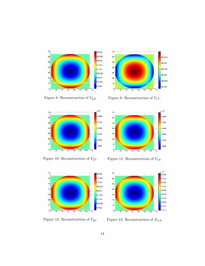
Figure 8: Reconstruction of VyA. Figure 9: Reconstruction of VxT .

Figure 10: Reconstruction of VyT . Figure 11: Reconstruction of VxV .

Figure 12: Reconstruction of VyV . Figure 13: Reconstruction of DxA.

14

Figure 14: Reconstruction of DxT . Figure 15: Reconstruction of DxV .

Example 2 In this last example we will analyze the radioactive tracer be-havior considering a slightly different case. The initial values correspondingto the parameters k1 and k2 have zeros in the central region, which visu-ally corresponds to the gaps shown on Figure 16. With this definition, weconsider the presence of something that hinders the flow, such as a tumor,for example. The new initial values used in this experiment and the per-formance of the algorithms for this instance are displayed in Table 4 andTable5, respectively.

Figure 16: Initial parameters k1 (left) and k2 (rigth) for Example 2.

These results showed a significant reduction in the number of iterationsand computer time. This reduction was approximately 98% for αk = 0.01,the step size by means of which we obtained the best results. Moreover, cansee in Figure 17 that the quality of the solution was preserved.

15

Table 4: Initial data for Example 2.

Parameter Initial Value (·)∗ a priori Regul. (α) Grad. Regul. (ξ)

k1 (1/cm) 0.90 (0) 0.89 0.017148965 0.0008k2 (1/cm) 0.75 (0) 0.70 0.016801553 0.0001k3 (1/cm) 0.01 0.85 0.051822197678965 0.0001VxA (cm/s) 1e-4 0.10 0.001024495 0.0001VyA (cm/s) 700.0 15.0 1.1 0.0001VxT (cm/s) -50.0 -5.0 1.22098745999 0.0001VyT (cm/s) 1e-4 0.10 0.001024495 0.0001VxV (cm/s) 1e-4 0.10 0.001024495 0.0001VyV (cm/s) 700.0 15.0 1.1000000001 0.0001DA (cm2/s) 3e-7 1e-3 0.0003344 0.000444DT (cm2/s) 3e-6 1e-2 0.000344 0.000444DV (cm2/s) 3e-7 1e-3 0.0003344 0.000444

Table 5: Performance of methods for Example 2.

αk = 0.1 αk = 0.01

NI TIME RES SENS NI TIME RES SENS

FBS 833 10734.3 6.3275 9.99e-5 833 10734.3 6.3275 9.99e-5BM1 2 52.6392 6.2407 9.93e-5 12 181.579 6.2069 9.61e-5BM2 2 53.1473 6.2407 9.93e-5 11 221.853 6.2711 9.95e-5

COLUM 2 52.6112 6.2410 9.93e-5 11 168.474 6.2714 9.95e-5ICOLUM 2 52.6392 6.2417 9.93e-5 11 169.674 6.2721 9.96e-5

THM 2 53.0833 6.2407 9.93e-5 11 170.190 6.2711 9.95e-5

0 200 400 600 8000

1

2

3

4

5

6

7

8x 10

−4

Número de iterações

sens

MB2 (t=0.01)MB2 (t=0.1)MB2 (t=1)FBS

0 200 400 600 80010

−3

10−2

10−1

100

101

Número de iterações

Res

íduo

MB2 (t=0.01)MB2 (t=0.1)MB2 (t=1)FBS

Figure 17: Convergence behavior of methods for Example 1.

16

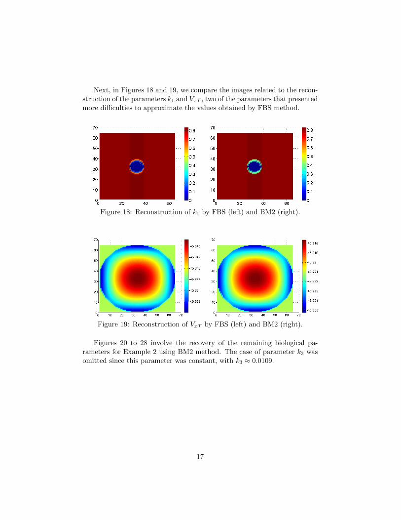
Next, in Figures 18 and 19, we compare the images related to the recon-struction of the parameters k1 and VxT , two of the parameters that presentedmore difficulties to approximate the values obtained by FBS method.

Figure 18: Reconstruction of k1 by FBS (left) and BM2 (right).

Figure 19: Reconstruction of VxT by FBS (left) and BM2 (right).

Figures 20 to 28 involve the recovery of the remaining biological pa-rameters for Example 2 using BM2 method. The case of parameter k3 wasomitted since this parameter was constant, with k3 ≈ 0.0109.

17

Figure 20: Reconstruction of k2. Figure 21: Reconstruction of VxA.

Figure 22: Reconstruction of VyA. Figure 23: Reconstruction of VyT .

Figure 24: Reconstruction of VxV . Figure 25: Reconstruction of VyV .

18

Figure 26: Reconstruction of DxA. Figure 27: Reconstruction of DxT .

Figure 28: Reconstruction of DxV .

In Figures 29-36, we display the concentration of radioactive material intissues CT and veins CV , and the image u, for different stages of time.

19

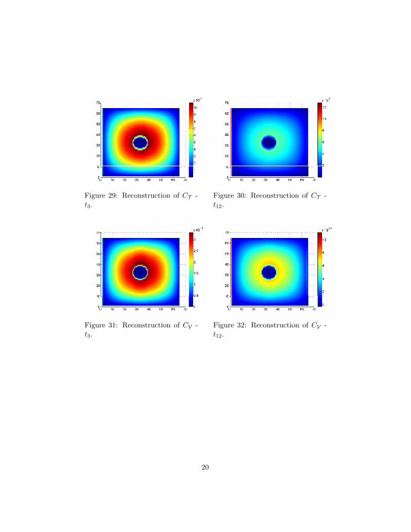
Figure 29: Reconstruction of CT -t3.

Figure 30: Reconstruction of CT -t12.

Figure 31: Reconstruction of CV -t3.

Figure 32: Reconstruction of CV -t12.

20

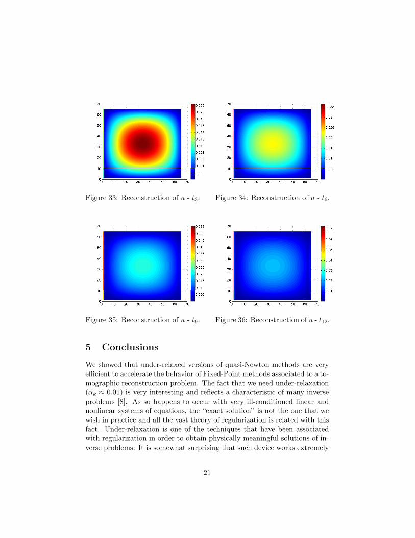
Figure 33: Reconstruction of u - t3. Figure 34: Reconstruction of u - t6.

Figure 35: Reconstruction of u - t9. Figure 36: Reconstruction of u - t12.

5 Conclusions

We showed that under-relaxed versions of quasi-Newton methods are veryefficient to accelerate the behavior of Fixed-Point methods associated to a to-mographic reconstruction problem. The fact that we need under-relaxation(αk ≈ 0.01) is very interesting and reflects a characteristic of many inverseproblems [8]. As so happens to occur with very ill-conditioned linear andnonlinear systems of equations, the “exact solution” is not the one that wewish in practice and all the vast theory of regularization is related with thisfact. Under-relaxation is one of the techniques that have been associatedwith regularization in order to obtain physically meaningful solutions of in-verse problems. It is somewhat surprising that such device works extremely

21

well when coupled to quasi-Newton acceleration.

6 Acknowledgements

The authors acknowledge the support for the present research provided byFAPESP, under Research Grant No. 2012/10444-0. We should like to thankProfessor Martin Burger (Institute for Computational and Applied Mathe-matics University of Munster) for useful suggestions about this paper.

References

[1] J. Y. Ahn, D. S. Lee, J. S. Lee, S. Kim, G. J. Cheon, J. S. Yeo, S. Shin,J. Chung, and M. C. Lee. Quantification of regional myocardial bloodflow using dynamic h15

2 o pet and factor analysis. Journal of NuclearMedicine, 42(5):782–787, 2001.

[2] M. Benning, P. Heins, M. Burger, T. E. Simos, G. Psihoyios, and C. Tsi-touras. A solver for dynamic pet reconstructions based on forward-backward-splitting. In AIP Conference Proceedings, volume 1281, pages1967–1970, 2010.

[3] M. Benning, T. Koesters, F. Wuebbeling, K. Schaefers, and M. Burger.A nonlinear variational method for improved quantification of myocar-dial blood flow using dynamic H15

2 O PET. IEEE Nuclear Science Sym-posium Conference, pages 4472–4477, 2008.

[4] S. R. Bergmann, K. A. Fox, A. L. Rand, K. D. McElvany, M. J. Welch,J. Markham, and B. E. Sobel. Quantification of regional myocardialblood flow in vivo with h15

2 o. Circulation, 70(4):724–733, 1984.

[5] M. Bierlaire and F. Crittin. Solving noisy, large-scale fixed-pointproblems and systems of nonlinear equations. Transportation Science,40(1):44–63, 2006.

[6] B. Blaschke, A. Neubauer, and O. Scherzer. On convergence ratesfor the iteratively regularized gauss-newton method. IMA Journal ofNumerical Analysis, 17:421–436, 1997.

[7] C. G. Broyden. A class of methods for solving nonlinear simultaneousequations. Mathematics of Computation, 19(92):577–593, 1965.

22

[8] C. L. Byrne. Iterative Optimization in Inverse Problems. CRC Press,2014.

[9] R. E. Carson. Positron Emission Tomography - Basic Sciences: TracerKinetic Modeling in PET. Springer, London, 2005.

[10] G. H-G. Chen and R. T. Rockafellar. Convergence rates in forward-backward splitting. SIAM Journal on Optimization, 7(2):421–444,1997.

[11] A. P. Dempster, N. M. Laird, and D. B. Rubin. Maximum likelihoodfrom incomplete data via the EM algorithm. Journal of the RoyalStatistical Society, 39:1–38, 1977.

[12] P. Deuflhard, R. Freund, and A. Walter. Fast secant methods for theiterative solution of large nonsymmetric linear systems. IMPACT ofComputing in Science and Engineering, 2(3):244–276, 1990.

[13] H. W. Engl E. Resmerita and A. N. Iusem. The expectation-maximization algorithm for ill-posed integral equations: a convergenceanalysis. Inverse Problems, 23(6):2575–2588, 2007.

[14] V. Eyert. A comparative study on methods for convergence accelera-tion of iterative vector sequences. Journal of Computational Physics,124(2):271–285, 1996.

[15] F. Wubbeling F. Natterer. Mathematical methods in image reconstruc-tion. Mathematical methods in image reconstruction, 2001.

[16] H. Fang and Y. Saad. Two classes of multisecant methods for nonlinearacceleration. Numerical Linear Algebra with Applications, 16(3):197–221, 2009.

[17] J. Hadamard. Lectures on Cauchy’s problem in linear partial differentialequations. Dover Publications, New York, 1953.

[18] M. Hanke. A regularizing levenberg-marquardt scheme, with appli-cations to inverse groundwater filtration problems. Inverse Problems,13:79–95, 1997.

[19] M. Hanke, A. Neubauer, and O. Scherzer. A convergence analysis ofthe landweber iteration for nonlinear ill-posed problems. NumerischeMatematik, (72):21–37, 1995.

23

[20] M. Jamshidian and R. I. Jennrich. Acceleration of the em algorithm byusing quasi-newton methods. Journal of the Royal Statistical Society:Series B (Statistical Methodology), 59(3):569–587, 1997.

[21] D. D. Johnson. Modified broyden’s method for accelerating convergencein self-consistent calculations. Physical Review B, 38(18):12807–12813,1988.

[22] B. Kaltenbacher. Some newton type methods for the regularization ofnonlinear ill posed problems. Inverse Problems, 13:729–753, 1997.

[23] M. E. Kamasak, C. A. Boumann, E. D. Morris, and K. Sauer. Directreconstruction of kinetic parameter images from dynamic PET data.IEEE Transactions on Medical Imaging, 24:636–650, 2005.

[24] K. Lange. A quasi-newton acceleration of the em algorithm. StatisticaSinica, 5(1):1–18, 1995.

[25] J. M. Libertini. Determining tumor blood flow parameters from dy-namic image measurements. In Journal of Physics: Conference Series,volume 135, page 012062, 2008.

[26] L. Ludemann, G. Sreenivasa, R. Michel, C. Rosner, M. Plotkin, R. Felix,P. Wust, and H. Amthauer. Corrections of arterial input function fordynamic h15

2 o pet to assess perfusion of pelvic tumours: arterial bloodsampling versus image extraction. Physics in medicine and biology,51(11):2883–2900, 2006.

[27] J. M. Martınez. A quasi-newton method with modification of one col-umn per iteration. Computing, 33(3-4):353–362, 1984.

[28] J. M. Martınez. Practical quasi-newton methods for solving nonlinearsystems. Journal of Computational and Applied Mathematics, 124:97–122, 2000.

[29] J. M. Martınez and M. C. Zambaldi. An inverse column-updatingmethod for solving large-scale nonlinear systems of equations. Opti-mization Methods and Software, 1:129–140, 1992.

[30] M. A. Mintun, M. E. Raichle, M. R. Kilbourn, G. F. Wooten, andM. J. Welch. A quantitative model for the in vivo assessment of drugbinding sites with positron emission tomography. Annals of neurology,15(3):217–227, 1984.

24

[31] M. A. Mintun, M. E. Raichle, W. R. Martin, and P. Herscovitch. Brainoxygen utilization measured with o-15 radiotracers and positron emis-sion tomography. Journal of nuclear medicine: official publication, So-ciety of Nuclear Medicine, 25(2):177–187, 1984.

[32] G. Muehllehner and J. S. Karp. Positron emission tomography. Physicsin medicine and biology, 51(13):R117–R137, 2006.

[33] Y. Nievergelt. The condition of steffensen’s acceleration in several vari-ables. Journal of Computational and Applied Mathematics, 58(3):291–305, 1995.

[34] J. M. Ollinger and J. A. Fessler. Positron-emission tomography. SignalProcessing Magazine, 14(1):43–55, 1997.

[35] R. Ramlau. A modified landweber-method for inverse problems. Nu-merical Functional Analysis and Optimization, 20, 1999.

[36] L. Reips. Parameter Identification in Medical Imaging. PhD thesis,Westfalische Wilhelms Universitat Munster, Munster, 2013.

[37] L. Reips, M. Burger, and R. Engbers. Towards dynamic pet reconstruc-tion under flow conditions: Parameter identification in a pde model.Journal of Inverse and Ill-Posed Problems, 2016. to appear.

[38] R. Saigal and M. J. Todd. Efficient acceleration techniques for fixedpoint algorithms. SIAM Journal on Numerical Analysis, 15(5):997–1007, 1978.

[39] G. P. Srivastava. Broyden’s method for self-consistent field conver-gence acceleration. Journal of Physics A: Mathematical and General,17(6):L317–L321, 1984.

[40] S. W. Thomas. Sequential estimation techniques for quasi-newton al-gorithms. Technical report, Cornell University, 1975.

[41] D. Vanderbilt and S. G. Louie. Total energies of diamond (111) sur-face reconstructions by a linear combination of atomic orbitals method.Physical Review B, 30(10):6118–6130, 1984.

[42] R. Varadhan and C. Roland. Simple and globally convergent methodsfor accelerating the convergence of any em algorithm. ScandinavianJournal of Statistics, 35(2):335–353, 2008.

25

[43] S. Villa, S. Salzo, L. Baldassarre, and A. Verri. Accelerated and in-exact forward-backward algorithms. SIAM Journal on Optimization,23(3):1607–1633, 2013.

[44] H. F. Walker and P. Ni. Anderson acceleration for fixed-point iterations.SIAM Journal on Numerical Analysis, 49(4):1715–1735, 2011.

[45] M. N. Wernick and J. N. Aarsvold. Emission Tomography: The Fun-damentals of PET and SPECT. Elsevier Academic Press, 2004.

[46] L. Kaufman Y. Vardi, L.A. Shepp. A statistical model for positron emis-sion tomography. J. of the American Statistical Association, 80(389):8–20, 1985.

[47] H. Zhou, D. Alexander, and K. Lange. A quasi-newton acceleration forhigh-dimensional optimization algorithms. Statistics and Computing,21(2):261–273, 2011.

26