Uncertainty-Aware Learning from Demonstration UsingMixture Density Networks with Sampling-Free Variance Modeling

Sungjoon Choi, Kyungjae Lee, Sungbin Lim, and Songhwai Oh

Abstract— In this paper, we propose an uncertainty-awarelearning from demonstration method by presenting a noveluncertainty estimation method utilizing a mixture densitynetwork appropriate for modeling complex and noisy humanbehaviors. The proposed uncertainty acquisition can be donewith a single forward path without Monte Carlo sampling andis suitable for real-time robotics applications. Then, we showthat it can be can be decomposed into explained variance andunexplained variance where the connections between aleatoricand epistemic uncertainties are addressed. The properties ofthe proposed uncertainty measure are analyzed through threedifferent synthetic examples, absence of data, heavy measure-ment noise, and composition of functions scenarios. We showthat each case can be distinguished using the proposed uncer-tainty measure and presented an uncertainty-aware learningfrom demonstration method of an autonomous driving usingthis property. The proposed uncertainty-aware learning fromdemonstration method outperforms other compared methodsin terms of safety using a complex real-world driving dataset.

I. INTRODUCTION

Recently, deep learning has been successfully appliedto a diverse range of research areas including computervision [1], natural language processing [2], and robotics[3]. When deep networks are kept in a cyber environmentwithout interacting with an actual physical system, mis-predictions or malfunctioning of the system may not causecatastrophic disasters. However, when using deep learningmethods in a real physical system involving human beings,such as an autonomous car, safety issues must be consideredappropriately [4].

In May 2016, in fact, a fatal car accident had occurreddue to the malfunctioning of a low-level image processingcomponent of an advanced assisted driving system (ADAS)to discriminate the white side of a trailer from a brightsky [5]. In this regard, Kendall and Gal [6] proposed anuncertainty modeling method for deep learning estimatingboth aleatoric and epistemic uncertainties indicating noiseinherent in the data generating process and uncertainty inthe predictive model which captures the ignorance aboutthe model. However, computationally-heavy Monte Carlosampling is required which makes it not suitable for real-time applications.

In this paper, we present a novel uncertainty estimationmethod for a regression task using a deep neural network andits application to learning from demonstration (LfD). Specifi-cally, a mixture density network (MDN) [7] is used to modelunderlying process which is more appropriate for describing

S. Choi, K. Lee, and S. Oh are with the Department of Elec-trical and Computer Engineering and ASRI, Seoul National Univer-sity, Seoul 08826, Korea (emails: {sungjoon.choi, kyungjae.lee, songh-wai.oh}@cpslab.snu.ac.kr). S. Lim is with the Department of Mathematics,Korea University (email: sungbin@korea.ac.kr).

complex distributions [8], e.g., human demonstrations. Wefirst present an uncertainty modeling method when makinga prediction with an MDN which can be acquired with asingle MDN forward path without Monte Carlo sampling.This sampling-free property makes it suitable for real-timerobotic applications compared to existing uncertainty mod-eling methods that require multiple models [9] or sampling[6], [10], [11]. Furthermore, as an MDN is appropriate formodeling complex distributions [12] compared to a densitynetwork used in [6], [12] or standard neural network forregression, the experimental results on autonomous drivingtell us that it can better represent the underlying policy of adriver given complex and noise demonstrations.

The main contributions of this paper are twofold. Wefirst present a sampling-free uncertainty estimation methodutilizing an MDN and show that it can be decomposedinto two parts, explained and unexplained variances whichindicate our ignorance about the model and measurementnoise, respectively. The properties of the proposed uncer-tainty modeling method is analyzed through three differentcases: absence of data, heavy measurement noise, and com-position of functions scenarios. Using the analysis, we furtherpropose an uncertainty-aware learning from demonstration(Lfd) method. We first train an aggressive controller in asimulated environment with an MDN and use the explainedvariance of an MDN to switch its mode to a rule-basedconservative controller. When applied to a complex real-world driving dataset from the US Highway 101 [13],the proposed uncertainty-award LfD outperforms comparedmethods in terms of safety of the driving as the out-of-distribution inputs, which are often refer to as covariate shift[14], are successfully captured by the proposed explainedvariance.

The remainder of this paper is composed as follows: Re-lated work and preliminaries regarding modeling uncertaintyin deep learning are introduced in Section II and Section III.The proposed uncertainty modeling method with an MDN ispresented in Section IV and analyzed in Section V. Finally,in Section VI, we present an uncertainty-aware learningfrom demonstration method and successfully apply to anautonomous driving task using a real-world driving datasetby deploying and controlling an virtual car inside the road.

II. RELATED WORK

Despite the heavy successes in deep learning researchareas, practical methods for estimating uncertainties in thepredictions with deep networks have only recently becomeactively studied. In the seminal study of Gal and Ghahramani[10], a practical method of estimating the predictive varianceof a deep neural network is proposed by computing from the

arX

iv:1

709.

0224

9v2

[cs

.CV

] 8

Sep

201

7

sample mean and variance of stochastic forward paths, i.e.,dropout [15]. The main contribution of [10] is to present aconnection between an approximate Bayesian network anda sparse Gaussian process. This method is often referred toas Monte Carlo (MC) dropout and successfully applied tomodeling model uncertainty in regression tasks, classificationtasks, and reinforcement learning with Thompson sampling.The interested readers are referred to [11] for more compre-hensive information about uncertainty in deep learning andBayesian neural networks.

Whereas [10] uses a standard neural network, [9] usesa density network whose output consists of both mean andvariance of a prediction trained with a negative log likelihoodcriterion. Adversarial training is also applied by incorporat-ing artificially generated adversarial examples. Furthermore,a multiple set of models are trained using different trainingsets to form an ensemble where the sample variance of amixture distribution is used to estimate the uncertainty ofa prediction. Interestingly, the usage of a mixture densitynetwork is encouraged in cases of modeling more complexdistributions. Guillaumes [8] compared existing uncertaintyacquisition methods including [9], [10].

Kendall and Gal [6] decomposed the predictive uncertaintyinto two major types, aleatoric uncertainty and epistemicuncertainty. First, epistemic uncertainty captures our igno-rance about the predictive model. It is often referred toas a reducible uncertainty as this type of uncertainty canbe reduced as we collect more training data from diversescenarios. On the other hand, aleatoric uncertainty capturesirreducible aspects of the predictive variance, such as therandomness inherent in the coin flipping. To this end, Kendalland Gal utilized a density network similar to [9] but used aslightly different cost function for numerical stability. Thevariance outputs directly from the density network indi-cates heteroscedastic aleatoric uncertainty where the overallpredictive uncertainty of the output y given an input x isapproximated using

V(y|x) ≈ 1

T

T∑t=1

µ2t (x)−

(T∑t=1

µt(x)

)2

+1

T

T∑t=1

σ(x) (1)

where {µt(x), σt(x)}Tt=1 are T samples of mean and vari-ance functions of a density network with stochastic forwardpaths.

Modeling and incorporating uncertainty in predictionshave been widely used in robotics, mostly to ensure safety inthe training phase of reinforcement learning [16] or to avoidfalse classification of learned cost function [17]. In [16], anuncertainty-aware collision prediction method is proposed bytraining multiple deep neural networks using bootstrappingand dropout. Once multiple networks are trained, the samplemean and variance of multiple stochastic forward pathsof different networks are used to compute the predictivevariance. Once the predictive variance is higher than a certainthreshold, a risk-averse cost function is used instead of thelearned cost function leading to a low-speed control. Thisapproach can be seen as extending [10] by adding addi-tional randomness from bootstrapping. However, as multiplenetworks are required, computational complexities of bothtraining and test phases are increased.

In [17], safe visual navigation is presented by traininga deep network for modeling the probability of collisionfor a receding horizon control problem. To handle out ofdistribution cases, a novelty detection algorithm is presentedwhere the reconstruction loss of an autoencoder is used asa measure of novelty. Once current visual input is detectedto be novel (high reconstruction loss), a rule-based collisionestimation is used instead of learning based estimation. Thisswitching between learning based and rule based approachesis similar to our approach. But, we focus on modeling anuncertainty of a policy function which consists of both inputand output pairs whereas the novelty detection in [17] canonly consider input data.

The proposed method can be regarded as extending pre-vious uncertainty estimation approaches by using a mixturedensity network (MDN) and present a novel variance esti-mation method for an MDN. We further show a single MDNwithout MC sampling is sufficient to model both reducibleand irreducible parts of uncertainty. In fact, we show thatit can better model both types of uncertainties in syntheticexamples.

III. PRELIMINARIES

A. Uncertainty Acquisition in Deep LearningIn [6], Kendall and Gal proposed two types of uncer-

tainties, aleatoric and epistemic uncertainties. These twotypes of uncertainties capture different aspects of predictiveuncertainty, i.e., a measure of uncertainty when we makea prediction using an approximation method such a deepnetwork. First, aleatoric uncertainty captures the uncertaintyin the data generating process, e.g., inherent randomness of acoin flipping or measurement noise. This type of uncertaintycannot be reduced even if we collect more training data. Onthe other hand, epistemic uncertainty models the ignoranceof the predictive model where it can be explained away givenan enough number of training data. Readers are referred toSection 6.7 in [11] for further details.

Let D = {(xi, yi) : i = 1, . . . , n} be a dataset of nsamples. For notational simplicity, we assume that an inputand output are an d-dimensional vector, i.e., x ∈ Rd, and ascalar, i.e., y ∈ R, respectively. Suppose that

y = f(x) + η

where f(·) is a target function and a measurement error ηfollows a zero-mean Gaussian distribution with a varianceσ2η , i.e., η ∼ N (0, σ2

η). Note that, in this case, the varianceof η corresponds to the aleatoric uncertainty, i.e., σ2

η = σ2a

where we will denote σ2a as aleatoric uncertainty. Similarly,

epistemic uncertainty will be denoted as σ2e .

Suppose that we train f(x) to approximate f(x) from Dand get

σ2e = E

∥∥∥f(x)− f(x)∥∥∥2 .

Then, we can see that

E∥∥∥y − f(x)

∥∥∥2 = E∥∥∥y − f(x) + f(x)− f(x)

∥∥∥2= E ‖y − f(x)‖2 + E

∥∥∥f(x)− f(x)∥∥∥2

= σ2a + σ2

e

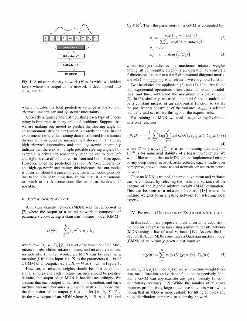
Fig. 1: A mixture density network (K = 3) with two hiddenlayers where the output of the network is decomposed intoπ, µ, and Σ.

which indicates the total predictive variance is the sum ofaleatoric uncertainty and epistemic uncertainty.

Correctly acquiring and distinguishing each type of uncer-tainty is important to many practical problems. Suppose thatwe are making our model to predict the steering angle ofan autonomous driving car (which is exactly the case in ourexperiments) where the training data is collected from humandrivers with an accurate measurement device. In this case,high aleatoric uncertainty and small epistemic uncertaintyindicate that there exist multiple possible steering angles. Forexample, a driver can reasonably steer the car to both leftand right in case of another car in front and both sides open.However, when the prediction has low aleatoric uncertaintyand high epistemic uncertainty, this indicates that our modelis uncertain about the current prediction which could possiblydue to the lack of training data. In this case, it is reasonableto switch to a risk-averse controller or alarm the driver, ifpossible.

B. Mixture Density Network

A mixture density network (MDN) was first proposed in[7] where the output of a neural network is composed ofparameters constructing a Gaussian mixture model (GMM):

p(y|θ) =

K∑j=1

πjN (y|µj , Σj)

where θ = {πj , µj ,Σj}Kj=1 is a set of parameters of a GMM,mixture probabilities, mixture means, and mixture variances,respectively. In other words, an MDN can be seen as amapping f from an input x ∈ X to the parameters θ ∈ Θ ofa GMM of an output, i.e., f : X 7→ Θ as shown in Figure 1.

However, as mixture weights should be on a K dimen-sional simplex and each mixture variance should be positivedefinite, the output of an MDN is handled accordingly. Weassume that each output dimension is independent, and eachmixture variance becomes a diagonal matrix. Suppose thatthe dimension of the output y is d and let {πj , µj , Σj}Kj=1

be the raw output of an MDN where πj ∈ R, µj ∈ Rd, and

Σj ∈ Rd. Then the parameters of a GMM is computed by

πj =exp (πj −max(π))∑Kk=1 exp(πk −max(π))

(2)

µj = µj

Σj = σmaxdiag(ρ(Σj)

)(3)

where max(π) indicates the maximum mixture weightsamong all K weights, diag(·) is an operation to convert ad-dimensional vector to a d×d-dimensional diagonal matrix,and ρ(x) = 1

1+exp(−x) is an element-wise sigmoid function.Two heuristics are applied in (2) and (3). First, we found

that exponential operations often cause numerical instabil-ities, and thus, subtracted the maximum mixture value in(2). In (3), similarly, we used a sigmoid function multipliedby a constant instead of an exponential function to satisfythe positiveness constraint of the variance. σmax is selectedmanually and set to five throughout the experiments.

For training the MDN, we used a negative log likelihoodas a cost function

c(θ;D) = − 1

N

N∑i=1

log(

K∑j=1

πj(xi)N (yi|µj(xi), Σj(xi))+ε)

(4)where D = {(xi,yi)}Ni=1 is a set of training data and ε =10−6 is for numerical stability of a logarithm function. Wewould like to note that an MDN can be implemented on topof any deep neural network architectures, e.g., a multi-layerperceptron, convolutional neural network, or recurrent neuralnetwork.

Once an MDN is trained, the predictive mean and variancecan be computed by selecting the mean and variance of themixture of the highest mixture weight (MAP estimation).This can be seen as a mixture of experts [18] where themixture weights form a gating network for selecting localexperts.

IV. PROPOSED UNCERTAINTY ESTIMATION METHOD

In this section, we propose a novel uncertainty acquisitionmethod for a regression task using a mixture density network(MDN) using a law of total variance [19]. As described inSection III-B, an MDN constitutes a Gaussian mixture model(GMM) of an output y given a test input x:

p(y|x) =

K∑j=1

πj(x)N (y;µj(x), Σj(x)) (5)

where πj(x), µj(x), and Σj(x) are j-th mixture weight func-tion, mean function, and variance function, respectively. Notethat a GMM can approximate any given density functionto arbitrary accuracy [12]. While the number of mixturesbecomes prohibitively large to achieve this, it is worthwhilenoting that an MDN is more suitable for fitting complex andnoisy distribution compared to a density network.

A. Uncertainty Acquisition for a Mixture Density Network

Let us first define the total expectation of a GMM.

E[y|x] =

K∑j=1

πj(x)

∫yN (y;µj(x),Σj(x))dy

=

K∑j=1

πj(x)µj(x) (6)

The total variance of a GMM is computed as follows (weomit x in each function).

V(y|x) =

∫‖y − E [y|x]‖2 p(y|x)dy

=

K∑j=1

πj

∫ ∥∥∥∥∥y −K∑k=1

πkµk

∥∥∥∥∥2

N (y;µj ,Σj)dy

where the term inside the integral becomes

∫ ∥∥∥∥∥y −K∑k=1

πkµk

∥∥∥∥∥2

N (y;µj ,Σj)dy

=

∫‖y − µj‖2N (y;µj ,Σj)dy

+

∫ ∥∥∥∥∥µj −K∑k=1

πkµk

∥∥∥∥∥2

N (y;µj ,Σj)dy

+ 2

∫(y − µj)T (µj −

K∑k=1

πkµk)N (y;µj ,Σj)dy

= Σj +

∥∥∥∥∥µj −K∑k=1

πkµk

∥∥∥∥∥2

.

Therefore the total variance V(y|x) becomes (also see (47)in [7]):

V(y|x) =

K∑j=1

πj(x)Σj(x)

+

K∑j=1

πj(x)

∥∥∥∥∥µj(x)−K∑k=1

πk(x)µk(x)

∥∥∥∥∥2

. (7)

Now let us present the connection between the two termsin (7) that constitute the total variance of a GMM to theepsitemic uncertainty and aleatoric uncertainty in [6].

B. Connection to Aleatoric and Epistemic Uncertainties

Let σa and σe be aleatoric uncertainty and epistemicuncertainty, respectively. Then, these two uncertainties con-stitute total predictive variance as shown in Section III-A.

V(y|x) = σ2a(x) + σ2

e (x)

On the other hand, we can rewrite (7) as

V (y|x) = Vk∼π (E [y|x, k]) + Ek∼π (V (y|x, k)) .

We remark that Vk∼π(E[y|x, k]) indicates explained vari-ance whereas Ek∼π [V(y|x, k)] represents unexplained vari-ance [19]. Observe that

Vk∼π(E[y|x, k]) = Vk∼π (µk(x))

=

K∑k=1

πk(x)

∥∥∥∥∥∥µk(x)−K∑j=1

πj(x)µj(x)

∥∥∥∥∥∥2

(8)

Ek∼π[V(y|x, k)] = Ek∼π [Σk(x)] =

K∑k=1

πk(x)Σk(x) (9)

This implies that (7) can be decomposed into uncertaintyquantity of each mixture, i.e.,

σ2a(x|k) + σ2

e (x|k)

= Σk(x) +

∥∥∥∥∥∥µk(x)−K∑j=1

πj(x)µj(x)

∥∥∥∥∥∥2

. (10)

Σk(x) in the right hand side of (10) is the predictedvariance of the k-th mixture where it can be interpretedas aleatoric uncertainty as the variance of a density net-work captures the noise inherent in data [16]. Consequently,∥∥∥µk(x)−

∑Kj=1 πj(x)µj(x)

∥∥∥2 corresponds to the epistemicuncertainty estimating our ignorance about the model pre-diction. We validate these connections with both syntheticexamples and track driving demonstrations in Section V andVI.

We would like to emphasize that Monte Carlo (MC)sampling is not required to compute the total variance ofa GMM as we introduced randomness from the mixturedistribution π. The predictive variance (1) proposed in in [6]requires MC sampling with random weight masking. Thisadditional sampling is required as the density network canonly model a single mean and variance. However, whenusing the MDN, it can not only model the measurementnoise or aleatoric uncertainty σ2

a with (9) but also model ourignorance about the model through (8). Intuitively speaking,(8) becomes high when the mean function of each mixturedoes not match the total expectation and will be used tomodel in uncertainty-aware learning from demonstration inSection VI.

V. ANALYSIS OF THE PROPOSED UNCERTAINTYMODELING WITH SYNTHETIC EXAMPLES

In this section, we analyze the properties of the proposeduncertainty modeling method in Section IV with three care-fully designed synthetic examples: absence of data, heavynoise, and composition of functions scenarios. In all exper-iments, fully connected networks with two hidden layers,256 hidden nodes, and tanh activation function1 is usedand the number of mixtures is 10. We also implementedthe algorithm in [6] with the same network topology andused 50 Monte Carlo (MC) sampling for computing the

1 Other activation functions such as relu or softplus had been testedas well but omitted as they showed poor regression performance onour problem. We also observe that increasing the number of mixturesover 10 does not affect the overall prediction and uncertainty estimationperformance.

(a) (b) (c) (d)

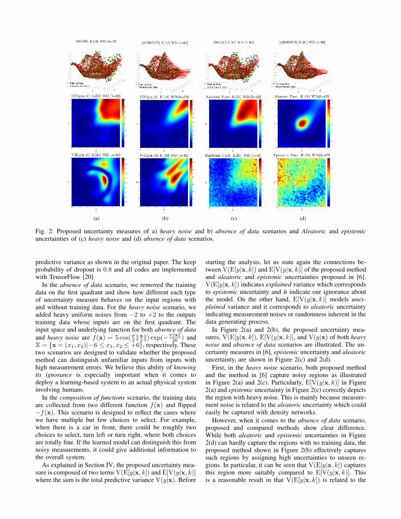
Fig. 2: Proposed uncertainty measures of a) heavy noise and b) absence of data scenarios and Aleatoric and epistemicuncertainties of (c) heavy noise and (d) absence of data scenarios.

predictive variance as shown in the original paper. The keepprobability of dropout is 0.8 and all codes are implementedwith TensorFlow [20]

In the absence of data scenario, we removed the trainingdata on the first quadrant and show how different each typeof uncertainty measure behaves on the input regions withand without training data. For the heavy noise scenario, weadded heavy uniform noises from −2 to +2 to the outputstraining data whose inputs are on the first quadrant. Theinput space and underlying function for both absence of dataand heavy noise are f(x) = 5 cos(π2 ‖

x2 ‖) exp(−π‖x‖20 ) and

X = {x = (x1, x2)|−6 ≤ x1, x2 ≤ +6}, respectively. Thesetwo scenarios are designed to validate whether the proposedmethod can distinguish unfamiliar inputs from inputs withhigh measurement errors. We believe this ability of knowingits ignorance is especially important when it comes todeploy a learning-based system to an actual physical systeminvolving humans.

In the composition of functions scenario, the training dataare collected from two different function f(x) and flipped−f(x). This scenario is designed to reflect the cases wherewe have multiple but few choices to select. For example,when there is a car in front, there could be roughly twochoices to select, turn left or turn right, where both choicesare totally fine. If the learned model can distinguish this fromnoisy measurements, it could give additional information tothe overall system.

As explained in Section IV, the proposed uncertainty mea-sure is composed of two terms V(E[y|x, k]) and E[V(y|x, k)]where the sum is the total predictive variance V(y|x). Before

starting the analysis, let us state again the connections be-tween V(E[y|x, k]) and E[V(y|x, k)] of the proposed methodand aleatoric and epistemic uncertainties proposed in [6].V(E[y|x, k]) indicates explained variance which correspondsto epistemic uncertainty and it indicate our ignorance aboutthe model. On the other hand, E[V(y|x, k)] models unex-plained variance and it corresponds to aleatoric uncertaintyindicating measurement noises or randomness inherent in thedata generating process.

In Figure 2(a) and 2(b), the proposed uncertainty mea-sures, V(E[y|x, k]), E[V(y|x, k)], and V(y|x) of both heavynoise and absence of data scenarios are illustrated. The un-certainty measures in [6], epistemic uncertainty and aleatoricuncertainty, are shown in Figure 2(c) and 2(d).

First, in the heavy noise scenario, both proposed methodand the method in [6] capture noisy regions as illustratedin Figure 2(a) and 2(c). Particularly, E[V(y|x, k)] in Figure2(a) and epistemic uncertainty in Figure 2(c) correctly depictsthe region with heavy noise. This is mainly because measure-ment noise is related to the aleatoric uncertainty which couldeasily be captured with density networks.

However, when it comes to the absence of data scenario,proposed and compared methods show clear difference.While both aleatoric and epistemic uncertainties in Figure2(d) can hardly capture the regions with no training data, theproposed method shown in Figure 2(b) effectively capturessuch regions by assigning high uncertainties to unseen re-gions. In particular, it can be seen that V(E[y|x, k]) capturesthis region more suitably compared to E[V(y|x, k)]. Thisis a reasonable result in that V(E[y|x, k]) is related to the

(a) (b) (c) (d) (e)

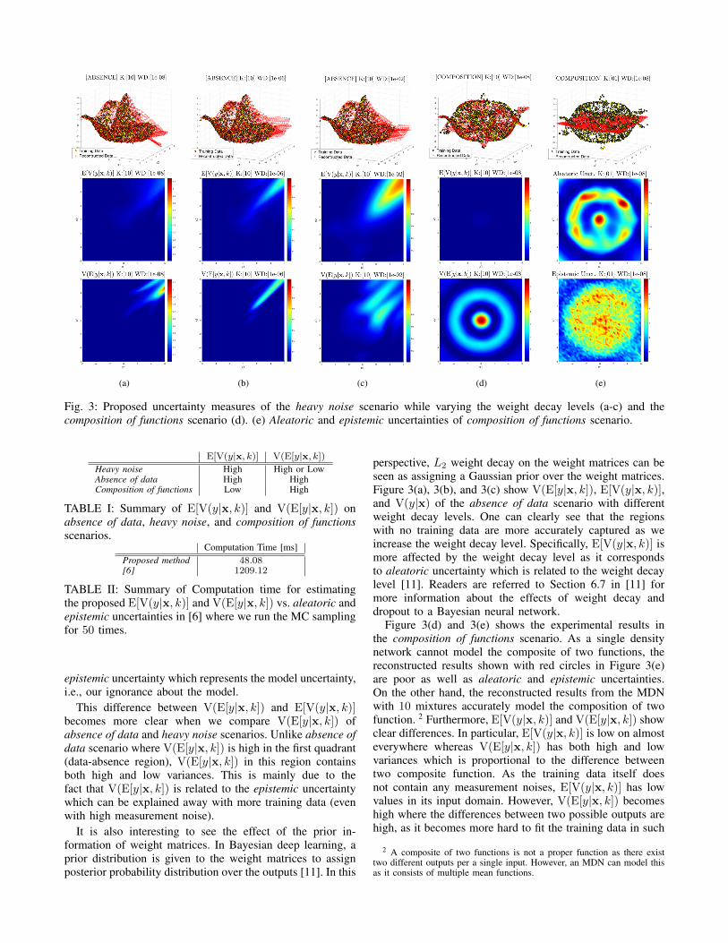
Fig. 3: Proposed uncertainty measures of the heavy noise scenario while varying the weight decay levels (a-c) and thecomposition of functions scenario (d). (e) Aleatoric and epistemic uncertainties of composition of functions scenario.

E[V(y|x, k)] V(E[y|x, k])Heavy noise High High or LowAbsence of data High HighComposition of functions Low High

TABLE I: Summary of E[V(y|x, k)] and V(E[y|x, k]) onabsence of data, heavy noise, and composition of functionsscenarios.

Computation Time [ms]Proposed method 48.08[6] 1209.12

TABLE II: Summary of Computation time for estimatingthe proposed E[V(y|x, k)] and V(E[y|x, k]) vs. aleatoric andepistemic uncertainties in [6] where we run the MC samplingfor 50 times.

epistemic uncertainty which represents the model uncertainty,i.e., our ignorance about the model.

This difference between V(E[y|x, k]) and E[V(y|x, k)]becomes more clear when we compare V(E[y|x, k]) ofabsence of data and heavy noise scenarios. Unlike absence ofdata scenario where V(E[y|x, k]) is high in the first quadrant(data-absence region), V(E[y|x, k]) in this region containsboth high and low variances. This is mainly due to thefact that V(E[y|x, k]) is related to the epistemic uncertaintywhich can be explained away with more training data (evenwith high measurement noise).

It is also interesting to see the effect of the prior in-formation of weight matrices. In Bayesian deep learning, aprior distribution is given to the weight matrices to assignposterior probability distribution over the outputs [11]. In this

perspective, L2 weight decay on the weight matrices can beseen as assigning a Gaussian prior over the weight matrices.Figure 3(a), 3(b), and 3(c) show V(E[y|x, k]), E[V(y|x, k)],and V(y|x) of the absence of data scenario with differentweight decay levels. One can clearly see that the regionswith no training data are more accurately captured as weincrease the weight decay level. Specifically, E[V(y|x, k)] ismore affected by the weight decay level as it correspondsto aleatoric uncertainty which is related to the weight decaylevel [11]. Readers are referred to Section 6.7 in [11] formore information about the effects of weight decay anddropout to a Bayesian neural network.

Figure 3(d) and 3(e) shows the experimental results inthe composition of functions scenario. As a single densitynetwork cannot model the composite of two functions, thereconstructed results shown with red circles in Figure 3(e)are poor as well as aleatoric and epistemic uncertainties.On the other hand, the reconstructed results from the MDNwith 10 mixtures accurately model the composition of twofunction. 2 Furthermore, E[V(y|x, k)] and V(E[y|x, k]) showclear differences. In particular, E[V(y|x, k)] is low on almosteverywhere whereas V(E[y|x, k]) has both high and lowvariances which is proportional to the difference betweentwo composite function. As the training data itself doesnot contain any measurement noises, E[V(y|x, k)] has lowvalues in its input domain. However, V(E[y|x, k]) becomeshigh where the differences between two possible outputs arehigh, as it becomes more hard to fit the training data in such

2 A composite of two functions is not a proper function as there existtwo different outputs per a single input. However, an MDN can model thisas it consists of multiple mean functions.

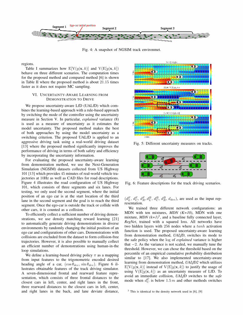
Fig. 4: A snapshot of NGSIM track environmet.

regions.Table I summarizes how E[V(y|x, k)] and V(E[y|x, k])

behave on three different scenarios. The computation timesfor the proposed method and compared method [6] is shownin Table II where the proposed method is about 21.15 timesfaster as it does not require MC sampling.

VI. UNCERTAINTY-AWARE LEARNING FROMDEMONSTRATION TO DRIVE

We propose uncertainty-aware LfD (UALfD) which com-bines the learning-based approach with a rule-based approachby switching the mode of the controller using the uncertaintymeasure in Section V. In particular, explained variance (8)is used as a measure of uncertainty as it estimates themodel uncertainty. The proposed method makes the bestof both approaches by using the model uncertainty as aswitching criterion. The proposed UALfD is applied to anaggressive driving task using a real-world driving dataset[13] where the proposed method significantly improves theperformance of driving in terms of both safety and efficiencyby incorporating the uncertainty information.

For evaluating the proposed uncertainty-aware learningfrom demonstration method, we use the Next-GenerationSimulation (NGSIM) datasets collected from US Highway101 [13] which provides 45 minutes of real-world vehicle tra-jectories at 10Hz as well as CAD files for road descriptions.Figure 4 illustrates the road configuration of US Highway101, which consists of three segments and six lanes. Fortesting, we only used the second segment, where the initialposition of an ego car is at the start location of the thirdlane in the second segment and the goal is to reach the thirdsegment. Once the ego-car is outside the track or collide withother cars, it is counted as a collision.

To efficiently collect a sufficient number of driving demon-strations, we use density matching reward learning [21]to automatically generate driving demonstrations in diverseenvironments by randomly changing the initial position of anego car and configurations of other cars. Demonstrations withcollisions are excluded from the dataset to form collision-freetrajectories. However, it is also possible to manually collectan efficient number of demonstrations using human-in-theloop simulations.

We define a learning-based driving policy π as a mappingfrom input features to the trigonometric encoded desiredheading angle of a car, (cos θdev, sin θdev). Figure 6 il-lustrates obtainable features of the track driving simulator.A seven-dimensional frontal and rearward feature repre-sentation, which consists of three frontal distances to theclosest cars in left, center, and right lanes in the front,three rearward distances to the closest cars in left, center,and right lanes in the back, and lane deviate distance,

Fig. 5: Different uncertainty measures on tracks.

Fig. 6: Feature descriptions for the track driving scenarios.

(dFL , dFC , d

FR, d

BL , d

BC , d

BR , ddev), are used as the input rep-

resentation.We trained three different network configurations: an

MDN with ten mixtures, MDN (K=10), MDN with onemixture, MDN (k=1)3, and a baseline fully connected layer,RegNet, trained with a squared loss. All networks havetwo hidden layers with 256 nodes where a tanh activationfunction is used. The proposed uncertainty-aware learningfrom demonstration method, UALfD, switches its mode tothe safe policy when the log of explained variance is higherthat −2. As the variance is not scaled, we manually tune thethreshold. However, we can chose the threshold based on thepercentile of an empirical cumulative probability distributionsimilar to [17]. We also implemented uncertainty-awarelearning from demonstration method, UALfD2 which utilizesE[V(y|x, k)] instead of V(E[y|x, k]) to justify the usage ofusing V(E[y|x, k]) as an uncertainty measure of LfD. Toavoid an immediate collision, UALfD switches to the safemode when dFC is below 1.5m and other methods switches

3 This is identical to the density network used in [6], [9]

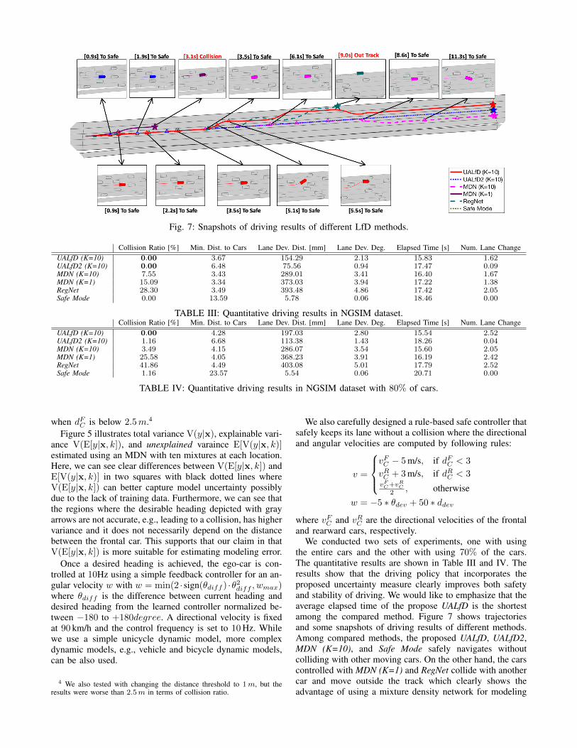
Fig. 7: Snapshots of driving results of different LfD methods.

Collision Ratio [%] Min. Dist. to Cars Lane Dev. Dist. [mm] Lane Dev. Deg. Elapsed Time [s] Num. Lane ChangeUALfD (K=10) 0.00 3.67 154.29 2.13 15.83 1.62UALfD2 (K=10) 0.00 6.48 75.56 0.94 17.47 0.09MDN (K=10) 7.55 3.43 289.01 3.41 16.40 1.67MDN (K=1) 15.09 3.34 373.03 3.94 17.22 1.38RegNet 28.30 3.49 393.48 4.86 17.42 2.05Safe Mode 0.00 13.59 5.78 0.06 18.46 0.00

TABLE III: Quantitative driving results in NGSIM dataset.Collision Ratio [%] Min. Dist. to Cars Lane Dev. Dist. [mm] Lane Dev. Deg. Elapsed Time [s] Num. Lane Change

UALfD (K=10) 0.00 4.28 197.03 2.80 15.54 2.52UALfD2 (K=10) 1.16 6.68 113.38 1.43 18.26 0.04MDN (K=10) 3.49 4.15 286.07 3.54 15.60 2.05MDN (K=1) 25.58 4.05 368.23 3.91 16.19 2.42RegNet 41.86 4.49 403.08 5.01 17.79 2.52Safe Mode 1.16 23.57 5.54 0.06 20.71 0.00

TABLE IV: Quantitative driving results in NGSIM dataset with 80% of cars.

when dFC is below 2.5m.4

Figure 5 illustrates total variance V(y|x), explainable vari-ance V(E[y|x, k]), and unexplained varaince E[V(y|x, k)]estimated using an MDN with ten mixtures at each location.Here, we can see clear differences between V(E[y|x, k]) andE[V(y|x, k)] in two squares with black dotted lines whereV(E[y|x, k]) can better capture model uncertainty possiblydue to the lack of training data. Furthermore, we can see thatthe regions where the desirable heading depicted with grayarrows are not accurate, e.g., leading to a collision, has highervariance and it does not necessarily depend on the distancebetween the frontal car. This supports that our claim in thatV(E[y|x, k]) is more suitable for estimating modeling error.

Once a desired heading is achieved, the ego-car is con-trolled at 10Hz using a simple feedback controller for an an-gular velocity w with w = min(2 · sign(θdiff ) ·θ2diff , wmax)where θdiff is the difference between current heading anddesired heading from the learned controller normalized be-tween −180 to +180degree. A directional velocity is fixedat 90 km/h and the control frequency is set to 10 Hz. Whilewe use a simple unicycle dynamic model, more complexdynamic models, e.g., vehicle and bicycle dynamic models,can be also used.

4 We also tested with changing the distance threshold to 1m, but theresults were worse than 2.5m in terms of collision ratio.

We also carefully designed a rule-based safe controller thatsafely keeps its lane without a collision where the directionaland angular velocities are computed by following rules:

v =

vFC − 5 m/s, if dFC < 3

vRC + 3 m/s, if dRC < 3vFC+vRC

2 , otherwise

w = −5 ∗ θdev + 50 ∗ ddev

where vFC and vRC are the directional velocities of the frontaland rearward cars, respectively.

We conducted two sets of experiments, one with usingthe entire cars and the other with using 70% of the cars.The quantitative results are shown in Table III and IV. Theresults show that the driving policy that incorporates theproposed uncertainty measure clearly improves both safetyand stability of driving. We would like to emphasize that theaverage elapsed time of the propose UALfD is the shortestamong the compared method. Figure 7 shows trajectoriesand some snapshots of driving results of different methods.Among compared methods, the proposed UALfD, UALfD2,MDN (K=10), and Safe Mode safely navigates withoutcolliding with other moving cars. On the other hand, the carscontrolled with MDN (K=1) and RegNet collide with anothercar and move outside the track which clearly shows theadvantage of using a mixture density network for modeling

human demonstrations. Furthermore, while both UALfD andUALfD2 navigate without a collision, the average elapsedtime and the average number lane changes varies greatly.This is mainly due to the fact that E[V(y|x, k)] captures themeasure noise rather than the model uncertainty which makesthe control conservative similar to that of the Safe Mode.

VII. CONCLUSION

In this paper, we proposed a novel uncertainty estimationmethod using a mixture density network. Unlike existingapproaches that rely on ensemble of multiple models orMonte Carlo sampling with stochastic forward paths, the pro-posed uncertainty acquisition method can run with a singlefeedforward model without computationally-heavy sampling.We show that the proposed uncertainty measure can bedecomposed into explained and unexplained variances andanalyze the properties with three different cases: absence ofdata, heavy measurement noise, and composition of functionsscenarios and show that it can effectively distinguish thethree cases using the two types of variances. Furthermore,we propose an uncertainty-aware learning from demonstra-tion method using the proposed uncertainty estimation andsuccessfully applied to real-world driving dataset.

REFERENCES

[1] K. He, X. Zhang, S. Ren, and J. Sun, “Deep residual learning for imagerecognition,” in Proc. of the IEEE conference on Computer Vision andPattern Recognition, 2016, pp. 770–778.

[2] R. Collobert and J. Weston, “A unified architecture for natural lan-guage processing: Deep neural networks with multitask learning,” inProc. of the International Conference on Machine Learning, 2008, pp.160–167.

[3] J. Schulman, S. Levine, P. Abbeel, M. I. Jordan, and P. Moritz, “Trustregion policy optimization.” in Proc. of the International Conferenceon Machine Learing, 2015, pp. 1889–1897.

[4] D. Amodei, C. Olah, J. Steinhardt, P. Christiano, J. Schulman,and D. Mane, “Concrete problems in ai safety,” arXiv preprintarXiv:1606.06565, 2016.

[5] AP and REUTERS, “Tesla working on ’improvements’ to its autopilotradar changes after model s owner became the first self-drivingfatality.” June 2016. [Online]. Available: https://goo.gl/XkzzQd

[6] A. Kendall and Y. Gal, “What uncertainties do we need in Bayesiandeep learning for computer vision?” arXiv preprint arXiv:1703.04977,2017.

[7] C. M. Bishop, “Mixture density networks,” 1994.[8] A. Brando Guillaumes, “Mixture density networks for distribution

and uncertainty estimation,” Master’s thesis, Universitat Politecnicade Catalunya, 2017.

[9] B. Lakshminarayanan, A. Pritzel, and C. Blundell, “Simple and scal-able predictive uncertainty estimation using deep ensembles,” arXivpreprint arXiv:1612.01474, 2016.

[10] Y. Gal and Z. Ghahramani, “Dropout as a Bayesian approximation:Representing model uncertainty in deep learning,” in Proc. of theInternational Conference on Machine Learing, 2016, pp. 1050–1059.

[11] Y. Gal, “Uncertainty in deep learning,” Ph.D. dissertation, PhD thesis,University of Cambridge, 2016.

[12] G. J. McLachlan and K. E. Basford, Mixture models: Inference andapplications to clustering. Marcel Dekker, 1988, vol. 84.

[13] J. Colyar and J. Halkias, “Us highway 101 dataset,” Federal HighwayAdministration (FHWA), Tech. Rep., 2007.

[14] S. Ross, “Interactive learning for sequential decisions and predictions,”Ph.D. dissertation, Carnegie Mellon University, 2013.

[15] N. Srivastava, G. E. Hinton, A. Krizhevsky, I. Sutskever, andR. Salakhutdinov, “Dropout: a simple way to prevent neural networksfrom overfitting.” Journal of machine learning research, vol. 15, no. 1,pp. 1929–1958, 2014.

[16] G. Kahn, A. Villaflor, V. Pong, P. Abbeel, and S. Levine, “Uncertainty-aware reinforcement learning for collision avoidance,” arXiv preprintarXiv:1702.01182, 2017.

[17] C. Richter and N. Roy, “Safe visual navigation via deep learningand novelty detection,” in Proc. of the Robotics: Science and SystemsConference, 2017.

[18] N. Shazeer, A. Mirhoseini, K. Maziarz, A. Davis, Q. Le, G. Hinton,and J. Dean, “Outrageously large neural networks: The sparsely-gatedmixture-of-experts layer,” arXiv preprint arXiv:1701.06538, 2017.

[19] R. O. Duda, P. E. Hart, and D. G. Stork, Pattern classification. Wiley,New York, 1973.

[20] M. Abadi, A. Agarwal, P. Barham, E. Brevdo, Z. Chen, C. Citro,G. S. Corrado, A. Davis, J. Dean, M. Devin et al., “Tensorflow: Large-scale machine learning on heterogeneous distributed systems,” arXivpreprint arXiv:1603.04467, 2016.

[21] S. Choi, K. Lee, A. Park, and S. Oh, “Density matching rewardlearning,” arXiv preprint arXiv:1608.03694, 2016.