an uncertainty-aware approach to optimal configuration of stream processing systems

AnUncertainty-AwareApproachtoOptimalConfigurationofStreamProcessingSystems

Pooyan Jamshidi, Giuliano CasaleImperial College [email protected]

MASCOTSLondon

19 Sept 2016

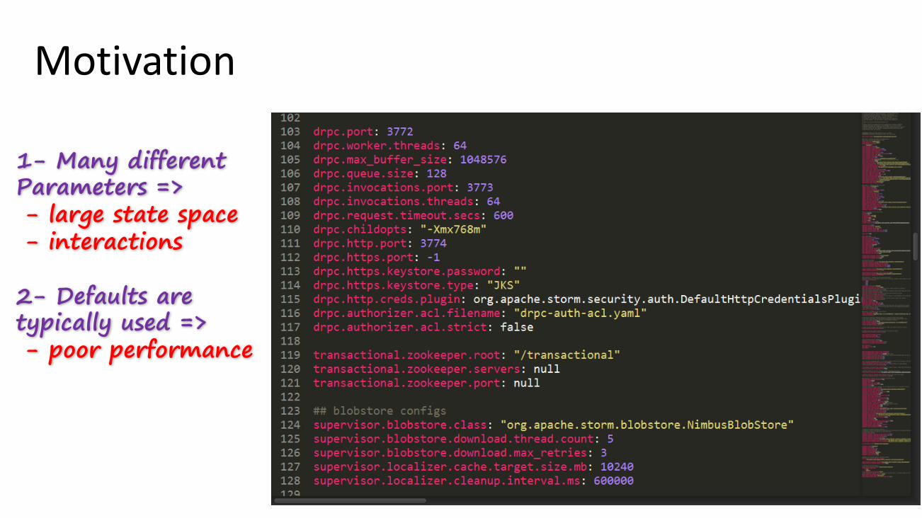
Motivation

1- Many different Parameters => - large state space- interactions

2- Defaults are typically used =>- poor performance

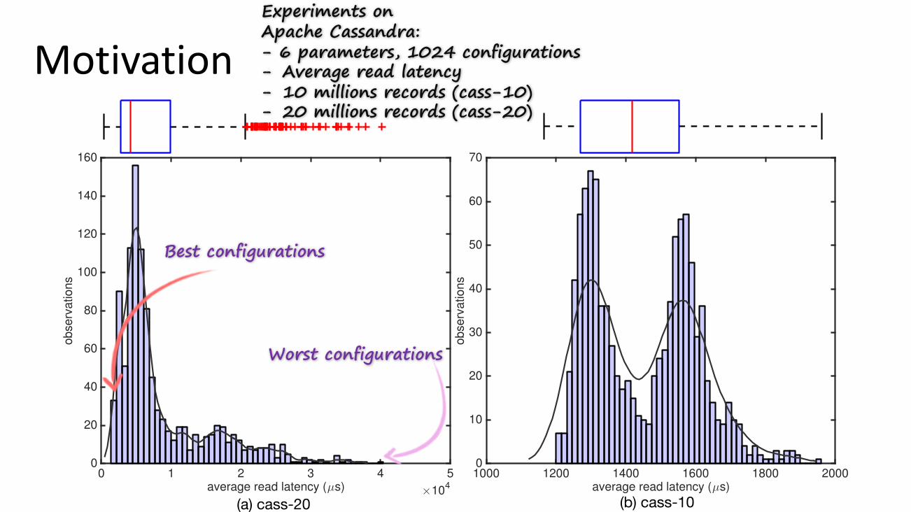
Motivation

0 1 2 3 4 5average read latency (µs)

×104

0

20

40

60

80

100

120

140

160

obse

rvatio

ns

1000 1200 1400 1600 1800 2000average read latency (µs)

0

10

20

30

40

50

60

70

obse

rvatio

ns

1

1200

1300

1400

1500

1600

1700

1800

1900

1

0.5 1

1.5 2

2.5 3

3.5 4

×10

4(a) cass-20 (b) cass-10

Best configurations

Worst configurations

Experiments on Apache Cassandra:- 6 parameters, 1024 configurations- Average read latency- 10 millions records (cass-10)- 20 millions records (cass-20)

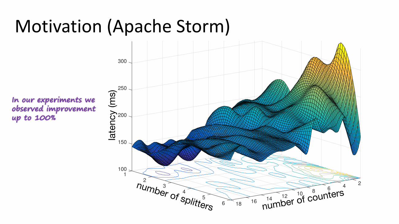
Motivation(ApacheStorm)

number of countersnumber of splitters

late

ncy

(ms)

100

150

1

200

250

2

300

Cubic Interpolation Over Finer Grid

243

684 10

125 14166 18

In our experiments we observed improvement up to 100%

Goal

information from the previous versions, the acquired data onthe current version, and apply a variety of kernel estimators[27] to locate regions where optimal configurations may lie.The key benefit of MTGPs over GPs is that the similaritybetween the response data helps the model to converge tomore accurate predictions much earlier. We experimentallyshow that TL4CO outperforms state-of-the-art configurationtuning methods. Our real configuration datasets are collectedfor three stream processing systems (SPS), implemented withApache Storm, a NoSQL benchmark system with ApacheCassandra, and using a dataset on 6 cloud-based clustersobtained in [21] worth 3 months of experimental time.The rest of this paper is organized as follows. Section 2

overviews the problem and motivates the work via an exam-ple. TL4CO is introduced in Section 3 and then validated inSection 4. Section 5 provides behind the scene and Section 6concludes the paper.

2. PROBLEM AND MOTIVATION

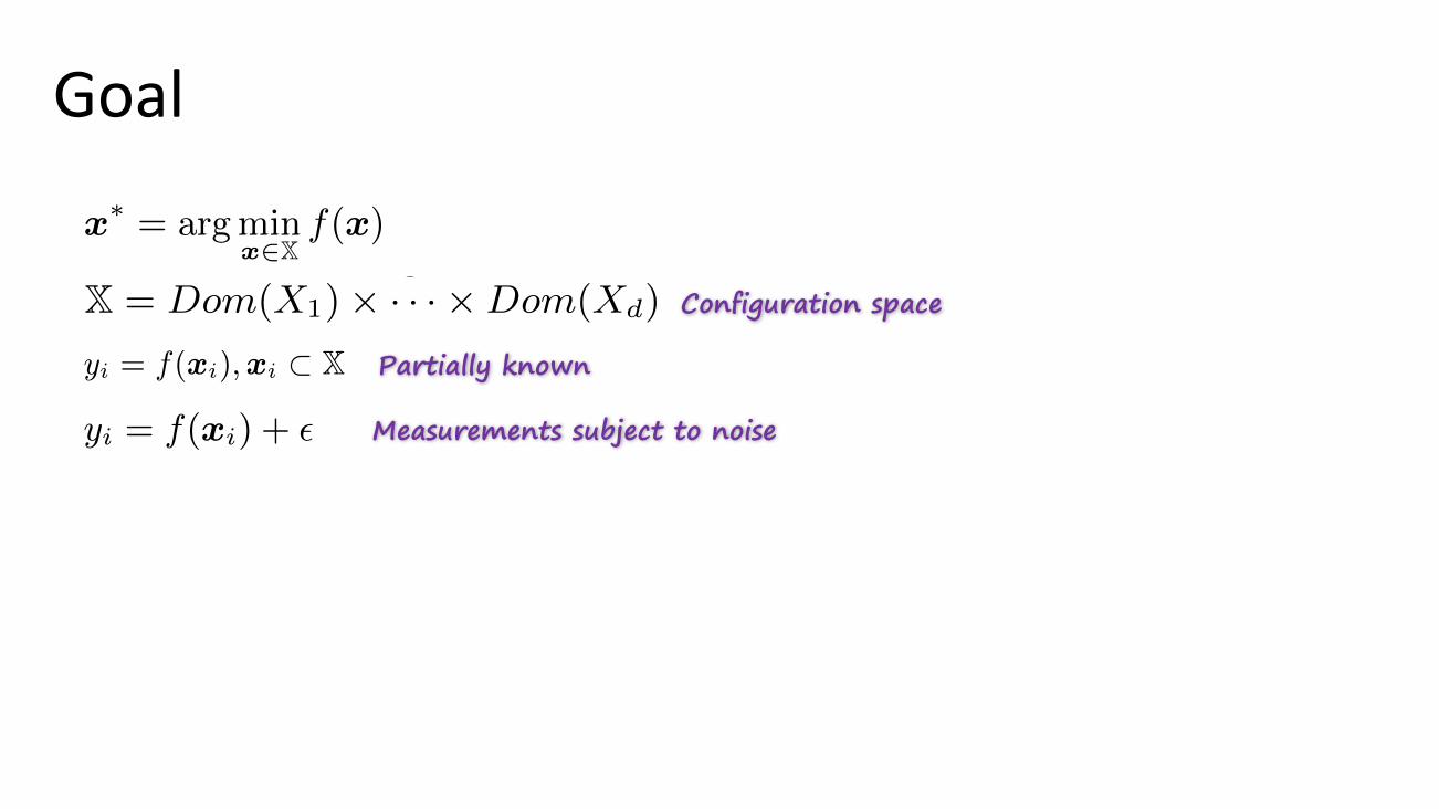
2.1 Problem statementIn this paper, we focus on the problem of optimal system

configuration defined as follows. Let Xi indicate the i-thconfiguration parameter, which ranges in a finite domainDom(Xi). In general, Xi may either indicate (i) integer vari-able such as level of parallelism or (ii) categorical variablesuch as messaging frameworks or Boolean variable such asenabling timeout. We use the terms parameter and factor in-terchangeably; also, with the term option we refer to possiblevalues that can be assigned to a parameter.

We assume that each configuration x 2 X in the configura-tion space X = Dom(X1)⇥ · · ·⇥Dom(Xd) is valid, i.e., thesystem accepts this configuration and the corresponding testresults in a stable performance behavior. The response withconfiguration x is denoted by f(x). Throughout, we assumethat f(·) is latency, however, other metrics for response maybe used. We here consider the problem of finding an optimalconfiguration x

⇤ that globally minimizes f(·) over X:

x

⇤ = argminx2X

f(x) (1)

In fact, the response function f(·) is usually unknown orpartially known, i.e., yi = f(xi),xi ⇢ X. In practice, suchmeasurements may contain noise, i.e., yi = f(xi) + ✏. Thedetermination of the optimal configuration is thus a black-box optimization program subject to noise [27, 33], whichis considerably harder than deterministic optimization. Apopular solution is based on sampling that starts with anumber of sampled configurations. The performance of theexperiments associated to this initial samples can delivera better understanding of f(·) and guide the generation ofthe next round of samples. If properly guided, the processof sample generation-evaluation-feedback-regeneration willeventually converge and the optimal configuration will belocated. However, a sampling-based approach of this kind canbe prohibitively expensive in terms of time or cost (e.g., rentalof cloud resources) considering that a function evaluation inthis case would be costly and the optimization process mayrequire several hundreds of samples to converge.

2.2 Related workSeveral approaches have attempted to address the above

problem. Recursive Random Sampling (RRS) [43] integratesa restarting mechanism into the random sampling to achievehigh search e�ciency. Smart Hill Climbing (SHC) [42] inte-grates the importance sampling with Latin Hypercube Design

(lhd). SHC estimates the local regression at each potentialregion, then it searches toward the steepest descent direction.An approach based on direct search [45] forms a simplexin the parameter space by a number of samples, and itera-tively updates a simplex through a number of well-definedoperations including reflection, expansion, and contractionto guide the sample generation. Quick Optimization viaGuessing (QOG) in [31] speeds up the optimization processexploiting some heuristics to filter out sub-optimal configu-rations. The statistical approach in [33] approximates thejoint distribution of parameters with a Gaussian in order toguide sample generation towards the distribution peak. Amodel-based approach [35] iteratively constructs a regressionmodel representing performance influences. Some approacheslike [8] enable dynamic detection of optimal configurationin dynamic environments. Finally, our earlier work BO4CO[21] uses Bayesian Optimization based on GPs to acceleratethe search process, more details are given later in Section 3.

2.3 SolutionAll the previous e↵orts attempt to improve the sampling

process by exploiting the information that has been gained inthe current task. We define a task as individual tuning cyclethat optimizes a given version of the system under test. As aresult, the learning is limited to the current observations andit still requires hundreds of sample evaluations. In this pa-per, we propose to adopt a transfer learning method to dealwith the search e�ciency in configuration tuning. Ratherthan starting the search from scratch, the approach transfersthe learned knowledge coming from similar versions of thesoftware to accelerate the sampling process in the currentversion. This idea is inspired from several observations arisein real software engineering practice [2, 3]. For instance, (i)in DevOps di↵erent versions of a system is delivered con-tinuously, (ii) Big Data systems are developed using similarframeworks (e.g., Apache Hadoop, Spark, Kafka) and runon similar platforms (e.g., cloud clusters), (iii) and di↵erentversions of a system often share a similar business logic.

To the best of our knowledge, only one study [9] exploresthe possibility of transfer learning in system configuration.The authors learn a Bayesian network in the tuning processof a system and reuse this model for tuning other similarsystems. However, the learning is limited to the structure ofthe Bayesian network. In this paper, we introduce a methodthat not only reuse a model that has been learned previouslybut also the valuable raw data. Therefore, we are not limitedto the accuracy of the learned model. Moreover, we do notconsider Bayesian networks and instead focus on MTGPs.

2.4 MotivationA motivating example. We now illustrate the previous

points on an example. WordCount (cf. Figure 1) is a popularbenchmark [12]. WordCount features a three-layer architec-ture that counts the number of words in the incoming stream.A Processing Element (PE) of type Spout reads the inputmessages from a data source and pushes them to the system.A PE of type Bolt named Splitter is responsible for splittingsentences, which are then counted by the Counter.

Kafka Spout Splitter Bolt Counter Bolt

(sentence) (word)[paintings, 3][poems, 60][letter, 75]

Kafka Topic

Stream to Kafka

File(sentence)

(sentence)

(sen

tenc

e)

Figure 1: WordCount architecture.

2








x

⇤ = argminx2X

f(x) (1)












Kafka Topic

Stream to Kafka

File(sentence)

(sentence)

(sen

tenc

e)


2








x

⇤ = argminx2X

f(x) (1)












Kafka Topic

Stream to Kafka

File(sentence)

(sentence)

(sen

tenc

e)


2








x

⇤ = argminx2X

f(x) (1)












Kafka Topic

Stream to Kafka

File(sentence)

(sentence)

(sen

tenc

e)


2

Partially known

Measurements subject to noise

Configuration space

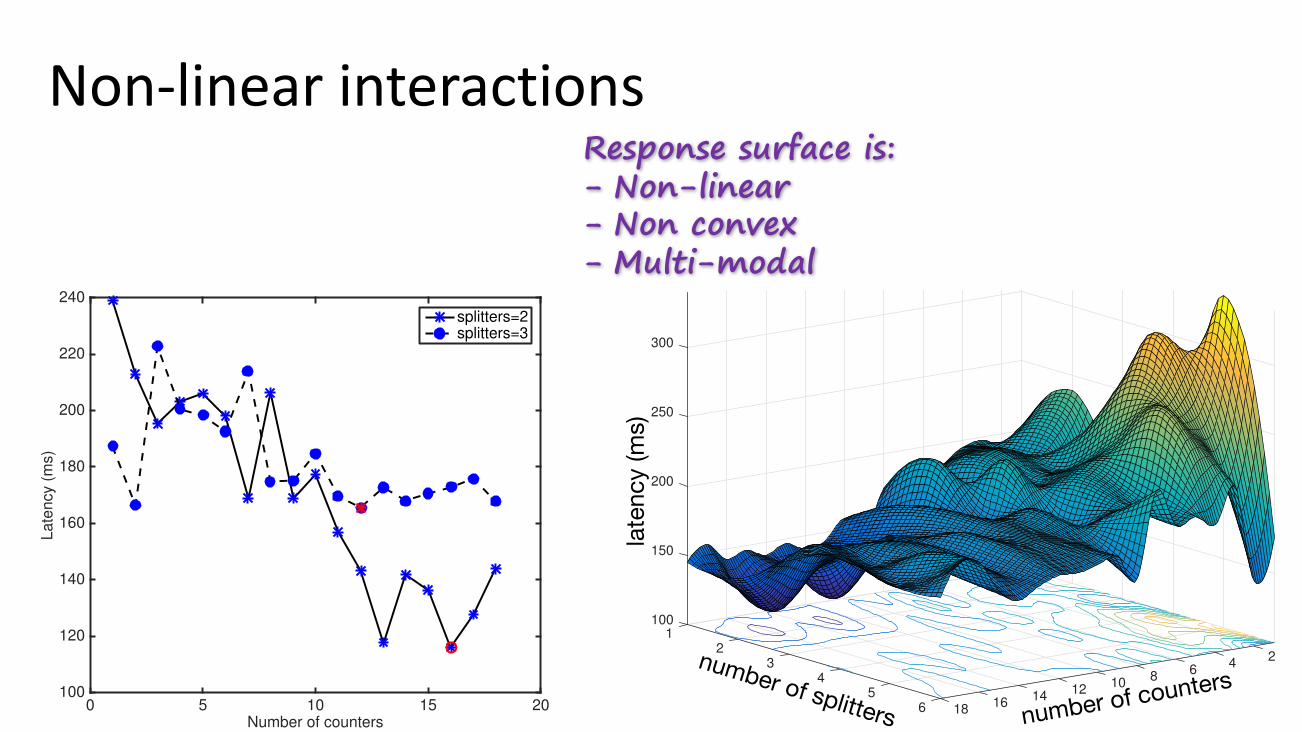
Non-linearinteractions

0 5 10 15 20Number of counters

100

120

140

160

180

200

220

240

Late

ncy

(m

s)

splitters=2splitters=3


late

ncy

(ms)

100

150

1

200

250

2

300


243

684 10

125 14166 18

Response surface is:- Non-linear- Non convex- Multi-modal

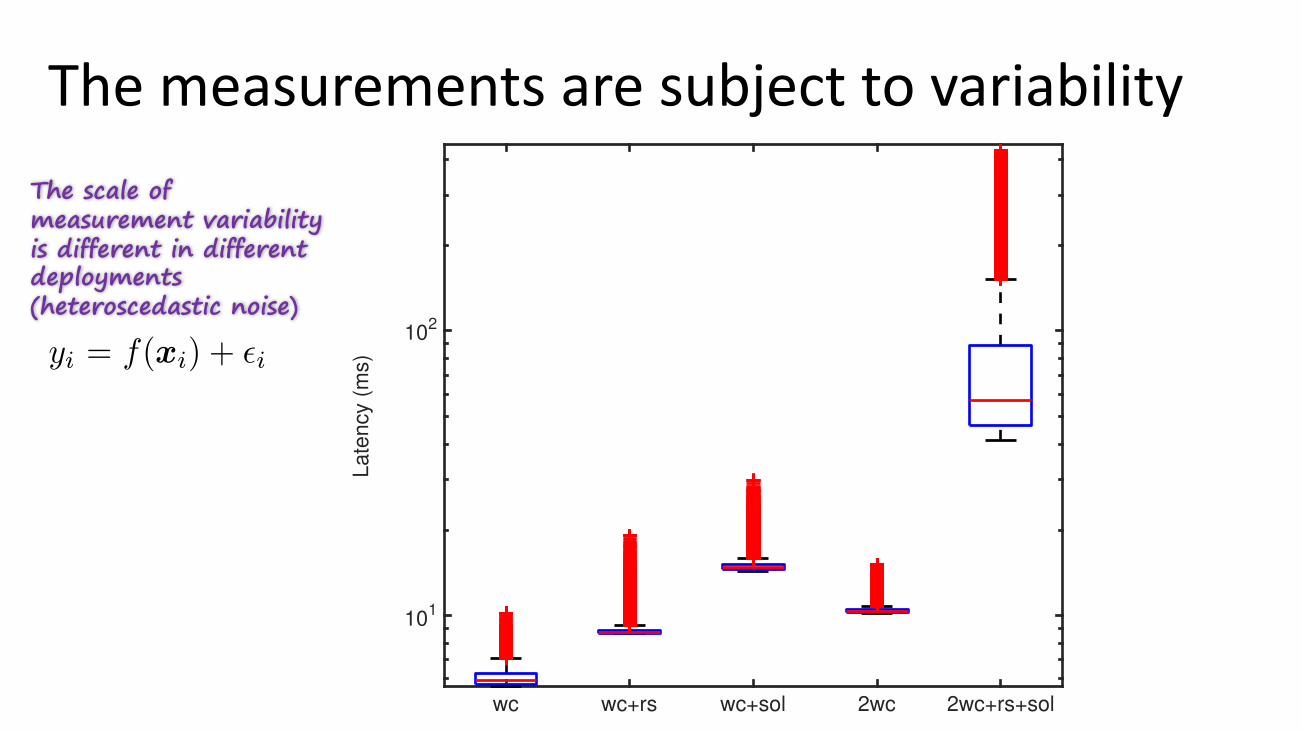
Themeasurementsaresubjecttovariability

wc wc+rs wc+sol 2wc 2wc+rs+sol

101

102

Late

ncy

(m

s)

The scale of measurement variability is different in different deployments (heteroscedastic noise)



Kafka Topic

Stream to Kafka

File(sentence)

(sentence)

(sen

tenc

e)

Fig. 1: WordCount topology architecture.

of d parameters of interest. We assume that each configurationx 2 X is valid and denote by f(x) the response measured onthe SPS under that configuration. Throughout, we assume thatf is latency, however other response metrics (e.g., throughput)may be used. The graph of f over configurations is calledthe response surface and it is partially observable, i.e., theactual value of f(x) is known only at points x that has beenpreviously experimented with. We here consider the problemof finding an optimal configuration x

⇤ that minimizes f overthe configuration space X with as few experiments as possible:

x

⇤= argmin

x2Xf(x) (1)

In fact, the response function f(·) is usually unknown orpartially known, i.e., y

i

= f(xi

),xi

⇢ X. In practice, suchmeasurements may contain noise, i.e., y

i

= f(xi

) + ✏i

. Notethat since the response surface is only partially-known, findingthe optimal configuration is a blackbox optimization problem[23], [29], which is also subject to noise. In fact, the problemof finding a optimal solution of a non-convex and multi-modalresponse surface (cf. Figure 2) is NP-hard [36]. Therefore, oninstances where it is impossible to locate a global optimum,BO4CO will strive to find the best possible local optimumwithin the available experimental budget.

B. Motivation1) A running example: WordCount (cf. Figure 1) is a

popular benchmark SPS. In WordCount a text file is fedto the system and it counts the number of occurrences ofthe words in the text file. In Storm, this corresponds to thefollowing operations. A Processing Element (PE) called Spoutis responsible to read the input messages (tuples) from a datasource (e.g., a Kafka topic) and stream the messages (i.e.,sentences) to the topology. Another PE of type Bolt calledSplitter is responsible for splitting sentences into words, whichare then counted by another PE called Counter.

2) Nonlinear interactions: We now illustrate one of theinherent challenges of configuration optimization. The metricthat defines the surface in Figure 2 is the latency of individualmessages, defined as the time since emission by the KafkaSpout to completion at the Counter, see Figure 1. Note thatthis function is the subset of wc(6D) in Table I when the levelof parallelism of Splitters and Counters is varied in [1, 6] and[1, 18]. The surface is strongly non-linear and multi-modaland indicates two important facts. First, the performancedifference between the best and worst settings is substantial,65%, and with more intense workloads we have observeddifferences in latency as large as 99%, see Table V. Next, non-linear relations between the parameters imply that the optimalnumber of counters depends on the number of Splitters, andvice-versa. Figure 3 shows this non-linear interaction [31] and


late

ncy

(ms)

100

150

1

200

250

2

300


243

684 10

125 14166 18

Fig. 2: WordCount response surface. It is an interpolated sur-face and is a projection of 6 dimensions, in wc(6D), onto 2D.It shows the non-convexity, multi-modality and the substantialperformance difference between different configurations.

0 5 10 15 20Number of counters

100

120

140

160

180

200

220

240

Late

ncy (

ms)

splitters=2splitters=3

Fig. 3: WordCount latency, cut though Figure 2.

demonstrates that if one tries to minimize latency by actingjust on one of these parameters at the time, the resultingconfiguration may not lead to a global optimum, as the numberof Splitters has a strong influence on the optimal counters.

3) Sparsity of effects: Another observation from our ex-tensive experiments with SPS is the sparsity of effects. Morespecifically, this means low-order interactions among a fewdominating factors can explain the main changes in the re-sponse function observed in the experiments. In this work weassume sparsity of effects, which also helps in addressing theintractable growth of the configuration space [19].

Methodology. In order to verify to what degree the sparsityof effects assumption holds in SPS, we ran experimentson 3 different benchmarks that exhibit different bottlenecks:WordCount (wc) is CPU intensive, RollingSort (rs) is mem-ory intensive, and SOL (sol) is network intensive. Differenttestbed settings were also considered, for a total of 5 datasets,as listed in Table I. Note that the parameters we considerhere are known to significantly influence latency, as they havebeen chosen according to professional tuning guides [26] andalso small scale tests where we varied a single parameter tomake sure that the selected parameters were all influential.For each test in the experiment, we run the benchmark for 8minutes including the initial burn-in period. Further detailson the experimental procedure are given in Section IV-B.Note that the largest dataset (i.e., rs(6D)) has required alone3840 ⇥ 8/60/24 = 21 days, within a total experimental timeof about 2.5 months to collect the datasets of Table I.

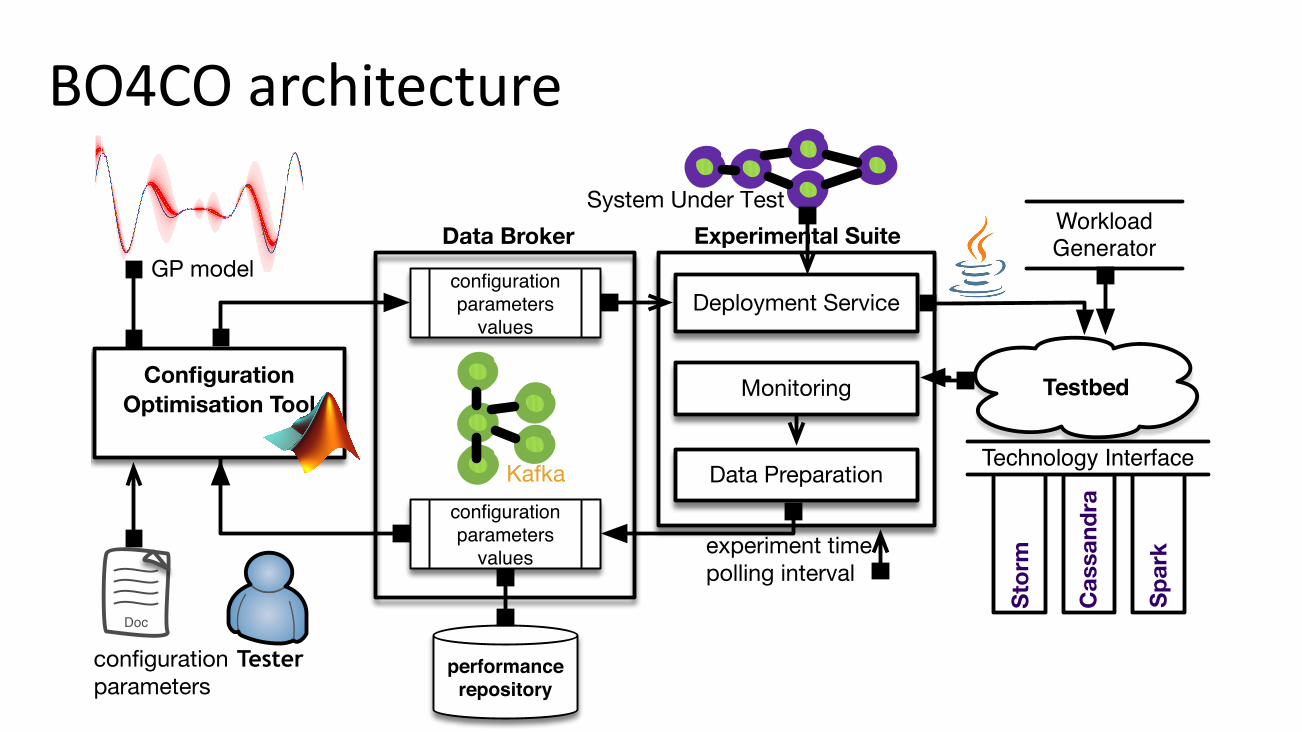
BO4COarchitecture

Configuration Optimisation Tool

performance repository

Monitoring

Deployment Service

Data Preparation

configuration parameters

values


values

Experimental Suite

Testbed

Doc

Data Broker

Tester

experiment timepolling interval

configurationparameters

GP model

Kafka

System Under TestWorkloadGenerator

Technology Interface

Stor

m

Cas

sand

ra

Spar

k

GPformodelingblackbox responsefunction

true function

GP mean

GP variance

observation

selected point

true minimum

Table 1: Pearson (Spearman) correlation coe�cients.v1 v2 v3 v4

v1 1 0.41 (0.49) -0.46 (-0.51) -0.50 (-0.51)v2 7.36E-06 (5.5E-08) 1 -0.20 (-0.2793) -0.18 (-0.24)v3 6.92E-07 (1.3E-08) 0.04 (0.003) 1 0.94 (0.88)v4 2.54E-08 (1.4E-08) 0.07 (0.01) 1.16E-52 (8.3E-36) 1

Table 2: Signal to noise ratios for WordCount.

Top. µ � µci �ciµ�

wc(v1) 516.59 7.96 [515.27, 517.90] [7.13, 9.01] 64.88wc(v2) 584.94 2.58 [584.51, 585.36] [2.32, 2.92] 226.32wc(v3) 654.89 13.56 [652.65, 657.13] [12.15, 15.34] 48.30wc(v4) 1125.81 16.92 [1123, 1128.6] [15.16, 19.14] 66.56

Figure 2 (a,b,c,d) shows the response surfaces for 4 di↵er-ent versions of the WordCount when splitters and countersare varied in [1, 6] and [1, 18]. WordCount v1, v2 (also v3, v4)are identical in terms of source code, but the environmentin which they are deployed on is di↵erent (we have deployedseveral other systems that compete for capacity in the samecluster). WordCount v1, v3 (also v2, v4) are deployed on a sim-ilar environment, but they have undergone multiple softwarechanges (we artificially injected delays in the source codeof its components). A number of interesting observationscan be made from the experimental results in Figure 2 andTables 1, 2 that we describe in the following subsections.

Correlation across di↵erent versions. We have measuredthe correlation coe�cients between the four versions of Word-Count in Table 1 (upper triangle shows the coe�cients whilelower triangle shows the p-values). The correlations be-tween the response functions are significant (p-values areless than 0.05). However, the correlation di↵ers betweenversions to versions. Also, more interestingly, di↵erent ver-sions of the system have di↵erent optimal configurations:x⇤v1 = (5, 1), x⇤

v2 = (6, 2), x⇤v3 = (2, 13), x⇤

v4 = (2, 16). InDevOps, di↵erent versions of a system will be delivered con-tinuously on daily basis [3]. Current DevOps practices donot systematically use the knowledge from previous versionsfor performance tuning of the current version under test de-spite such significant correlations [3]. There are two reasonsbehind this: (i) the techniques that are used for performancetuning cannot exploit the historical data belong to a di↵erentversion. (ii) they assume di↵erent versions have the sameoptimum configuration. However, based on our experimentalobservations above, this is not true. As a result, the existingpractice treat the experimental data as one-time-use.

Nonlinear interactions. The response functions f(·) in Fig-ure 2 are strongly non-linear, non-convex and multi-modal.The performance di↵erence between the best and worst set-tings is substantial, e.g., 65% in v4, providing a case foroptimal tuning. Moreover, the non-linear relations amongthe parameters imply that the optimal number of countersdepends on splitters, and vice-versa. In other words, if onetries to minimize latency by acting just on one of theseparameters, this may not lead to a global optimum [21].Measurement uncertainty. We have taken samples of the

latency for the same configuration (splitters=counters=1) ofthe 4 versions of WordCount. The experiment were conductedon Amazon EC2 (m3.large (2 CPU, 7.5 GB)). After filteringthe initial burn-in, we have computed average and variance ofthe measurements. The results in Table 2 illustrate that thevariability of measurements across di↵erent versions can beof di↵erent scales. In traditional techniques, such as designof experiments, the variability is typically disregarded byrepeating experiments and obtaining the mean. However, wehere pursue an alternative approach that relies on MTGPmodels that are able to explicitly take into account variability.

3. TL4CO: TRANSFER LEARNING FOR CON-FIGURATION OPTIMIZATION

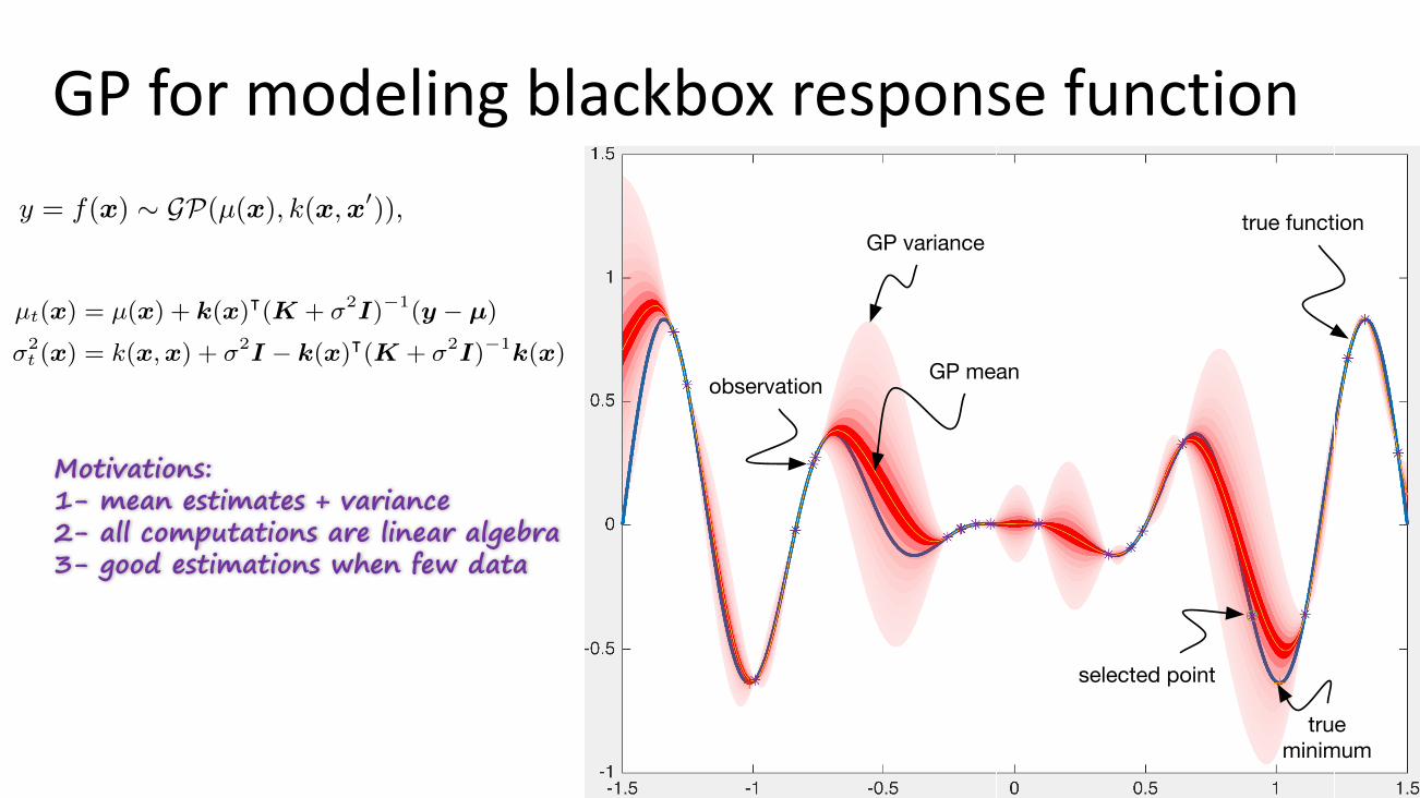
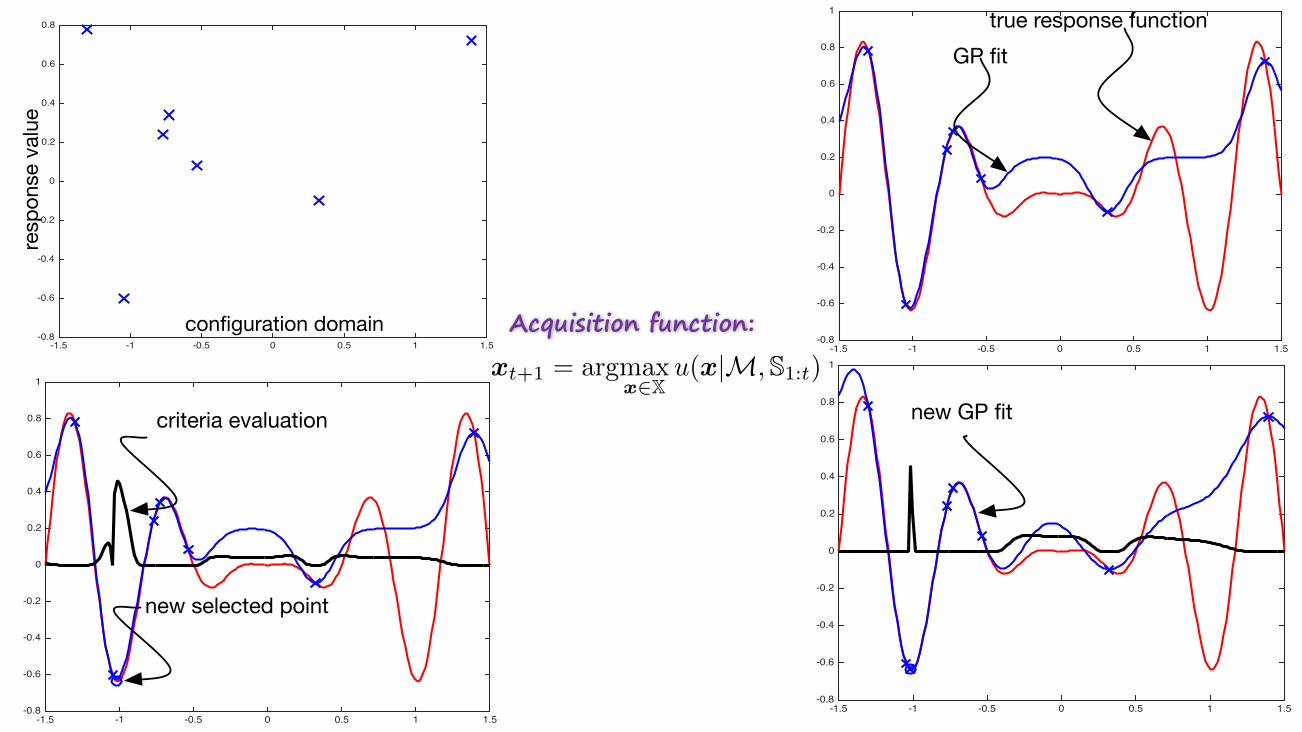
3.1 Single-task GP Bayesian optimizationBayesian optimization [34] is a sequential design strategy

that allows us to perform global optimization of black-boxfunctions. Figure 3 illustrates the GP-based Bayesian Op-timization approach using a 1-dimensional response. Thecurve in blue is the unknown true response, whereas themean is shown in yellow and the 95% confidence interval ateach point in the shaded red area. The stars indicate ex-perimental measurements (or observation interchangeably).Some points x 2 X have a large confidence interval due tolack of observations in their neighborhood, while others havea narrow confidence. The main motivation behind the choiceof Bayesian Optimization here is that it o↵ers a frameworkin which reasoning can be not only based on mean estimatesbut also the variance, providing more informative decisionmaking. The other reason is that all the computations inthis framework are based on tractable linear algebra.In our previous work [21], we proposed BO4CO that ex-

ploits single-task GPs (no transfer learning) for prediction ofposterior distribution of response functions. A GP model iscomposed by its prior mean (µ(·) : X ! R) and a covariancefunction (k(·, ·) : X⇥ X ! R) [41]:

y = f(x) ⇠ GP(µ(x), k(x,x0)), (2)

where covariance k(x,x0) defines the distance between x

and x

0. Let us assume S1:t = {(x1:t, y1:t)|yi := f(xi)} bethe collection of t experimental data (observations). In thisframework, we treat f(x) as a random variable, conditionedon observations S1:t, which is normally distributed with thefollowing posterior mean and variance functions [41]:

µt(x) = µ(x) + k(x)|(K + �2I)�1(y � µ) (3)

�2t (x) = k(x,x) + �2

I � k(x)|(K + �2I)�1

k(x) (4)

where y := y1:t, k(x)| = [k(x,x1) k(x,x2) . . . k(x,xt)],

µ := µ(x1:t), K := k(xi,xj) and I is identity matrix. Theshortcoming of BO4CO is that it cannot exploit the observa-tions regarding other versions of the system and as thereforecannot be applied in DevOps.

3.2 TL4CO: an extension to multi-tasksTL4CO 1 uses MTGPs that exploit observations from other

previous versions of the system under test. Algorithm 1defines the internal details of TL4CO. As Figure 4 shows,TL4CO is an iterative algorithm that uses the learning fromother system versions. In a high-level overview, TL4CO: (i)selects the most informative past observations (details inSection 3.3); (ii) fits a model to existing data based on kernellearning (details in Section 3.4), and (iii) selects the nextconfiguration based on the model (details in Section 3.5).

In the multi-task framework, we use historical data to fit abetter GP providing more accurate predictions. Before that,we measure few sample points based on Latin Hypercube De-sign (lhd) D = {x1, . . . , xn} (cf. step 1 in Algorithm 1). Wehave chosen lhd because: (i) it ensures that the configurationsamples in D is representative of the configuration space X,whereas traditional random sampling [26, 17] (called brute-force) does not guarantee this [29]; (ii) another advantage isthat the lhd samples can be taken one at a time, making it e�-cient in high dimensional spaces. We define a new notation for1Code+Data will be released (due in July 2016), as this isfunded under the EU project DICE: https://github.com/dice-project/DICE-Configuration-BO4CO

3


v1 1 0.41 (0.49) -0.46 (-0.51) -0.50 (-0.51)v2 7.36E-06 (5.5E-08) 1 -0.20 (-0.2793) -0.18 (-0.24)v3 6.92E-07 (1.3E-08) 0.04 (0.003) 1 0.94 (0.88)v4 2.54E-08 (1.4E-08) 0.07 (0.01) 1.16E-52 (8.3E-36) 1



wc(v1) 516.59 7.96 [515.27, 517.90] [7.13, 9.01] 64.88wc(v2) 584.94 2.58 [584.51, 585.36] [2.32, 2.92] 226.32wc(v3) 654.89 13.56 [652.65, 657.13] [12.15, 15.34] 48.30wc(v4) 1125.81 16.92 [1123, 1128.6] [15.16, 19.14] 66.56



v2 = (6, 2), x⇤v3 = (2, 13), x⇤








y = f(x) ⇠ GP(µ(x), k(x,x0)), (2)


and x


µt(x) = µ(x) + k(x)|(K + �2I)�1(y � µ) (3)

�2t (x) = k(x,x) + �2

I � k(x)|(K + �2I)�1

k(x) (4)






3

Motivations:1- mean estimates + variance2- all computations are linear algebra3- good estimations when few data

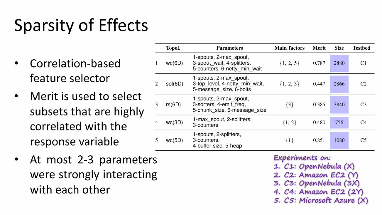
SparsityofEffects

• Correlation-basedfeature selector

• Meritisusedtoselectsubsetsthatarehighlycorrelatedwiththeresponsevariable

• At most 2-3 parameterswere strongly interactingwith each other

TABLE I: Sparsity of effects on 5 experiments where we have varieddifferent subsets of parameters and used different testbeds. Note thatthese are the datasets we experimentally measured on the benchmarksystems and we use them for the evaluation, more details includingthe results for 6 more experiments are in the appendix.

Topol. Parameters Main factors Merit Size Testbed

1 wc(6D)1-spouts, 2-max spout,3-spout wait, 4-splitters,5-counters, 6-netty min wait

{1, 2, 5} 0.787 2880 C1

2 sol(6D)1-spouts, 2-max spout,3-top level, 4-netty min wait,5-message size, 6-bolts

{1, 2, 3} 0.447 2866 C2

3 rs(6D)1-spouts, 2-max spout,3-sorters, 4-emit freq,5-chunk size, 6-message size

{3} 0.385 3840 C3

4 wc(3D) 1-max spout, 2-splitters,3-counters {1, 2} 0.480 756 C4

5 wc(5D)1-spouts, 2-splitters,3-counters,4-buffer-size, 5-heap

{1} 0.851 1080 C5

wc wc+rs wc+sol 2wc 2wc+rs+sol

101

102

Late

ncy

(m

s)

Fig. 4: Noisy experimental measurements. Note that + heremeans that wc is deployed in a multi-tenant environmentwith other topologies and as a result not only the latency isincreased but also the variability became greater.

Results. After collecting experimental data, we have useda common correlation-based feature selector1 implemented inWeka to rank parameter subsets according to a heuristic. Thebias of the merit function is toward subsets that contain pa-rameters that are highly correlated with the response variable.Less influential parameters are filtered because they will havelow correlation with latency, and a set with the main factorsis returned. For all of the 5 datasets, we list in Table I themain factors. The analysis results demonstrate that in all the 5experiments at most 2-3 parameters were strongly interactingwith each other, out of a maximum of 6 parameters variedsimultaneously. Therefore, the determination of the regionswhere performance is optimal will likely be controlled by suchdominant factors, even though the determination of a globaloptimum will still depends on all the parameters.

4) Measurement uncertainty: We now illustrate measure-ment variabilities, which represent an additional challenge forconfiguration optimization. As depicted in Figure 4, we took

1The most significant parameters are selected based on the following meritfunction [9], also shown in Table I:

mps =nrlpp

n+ n(n� 1)rpp, (2)

where rlp is the mean parameter-latency correlation, n is the number ofparameters, rpp is the average feature-feature inter-correlation [9, Sec 4.4].

different samples of the latency metric over 2 hours for fivedifferent deployments of WordCount. The experiments runon a multi-node cluster on the EC2 cloud. After filtering theinitial burn-in, we computed averages and standard deviationof the latencies. Note that the configuration across all 5settings is similar, the only difference is the number of co-located topologies in the testbed. The data in boxplots illustratethat variability can be small in some settings (e.g., wc),while they can be large in some other experimental setups(e.g., 2wc+rs+sol). In traditional techniques such as designof experiments, such variability is addressed by repeatingexperiments multiple times and obtaining regression estimatesfor the system model across such repetitions. However, wehere pursue the alternative approach of relying on GP modelsto capture both mean and variance of measurements withinthe model that guides the configuration process. The theoryunderpinning this approach is discussed in the next section.

III. BO4CO: BAYESIAN OPTIMIZATION FORCONFIGURATION OPTIMIZATION

A. Bayesian Optimization with Gaussian Process prior

Bayesian optimization is a sequential design strategy thatallows us to perform global optimization of blackbox functions[30]. The main idea of this method is to treat the blackboxobjective function f(x) as a random variable with a given priordistribution, and then perform optimization on the posteriordistribution of f(x) given experimental data. In this work,GPs are used to model this blackbox objective function at eachpoint x 2 X. That is, let S1:t be the experimental data collectedin the first t iterations and let x

t+1 be a candidate configurationthat we may select to run the next experiment. Then BO4COassesses the probability that this new experiment could findan optimal configuration using the posterior distribution:

Pr(ft+1|S1:t,xt+1) ⇠ N (µ

t

(x

t+1),�2t

(x

t+1)),

where µt

(x

t+1) and �2t

(x

t+1) are suitable estimators of themean and standard deviation of a normal distribution that isused to model this posterior. The main motivation behind thechoice of GPs as prior here is that it offers a framework inwhich reasoning can be not only based on mean estimatesbut also the variance, providing more informative decisionmakings. The other reason is that all the computations in thisframework are based on linear algebra.

Figure 5 illustrates the GP-based Bayesian optimizationusing a 1-dimensional response surface. The curve in blue isthe unknown true posterior distribution, whereas the mean isshown in green and the 95% confidence interval at each pointin the shaded area. Stars indicate measurements carried out inthe past and recorded in S1:t (i.e., observations). Configurationcorresponds to x1 has a large confidence interval due to lack ofobservations in its neighborhood. Conversely, x4 has a narrowconfidence since neighboring configurations have been exper-imented with. The confidence interval in the neighborhood ofx2 and x3 is not high and correctly our approach does notdecide to explore these zones. The next configuration x

t+1,indicated by a small circle right to the x4, is selected basedon a criterion that will be defined later.

Experiments on:1. C1: OpenNebula (X)2. C2: Amazon EC2 (Y)3. C3: OpenNebula (3X)4. C4: Amazon EC2 (2Y)5. C5: Microsoft Azure (X)

-1.5 -1 -0.5 0 0.5 1 1.5-1.5

-1

-0.5

0

0.5

1

x1 x2 x3 x4

true function

GP surrogate mean estimate

observation

Fig. 5: An example of 1D GP model: GPs provide mean esti-mates as well as the uncertainty in estimations, i.e., variance.



Monitoring

Deployment Service

Data Preparation


values


values

Experimental Suite

Testbed

Doc

Data Broker

Tester



GP model

Kafka



Stor

m

Cas

sand

ra

Spar

k

Fig. 6: BO4CO architecture: (i) optimization and (ii) exper-imental suite are integrated via (iii) a data broker. The in-tegrated solution is available: https://github.com/dice-project/DICE-Configuration-BO4CO.

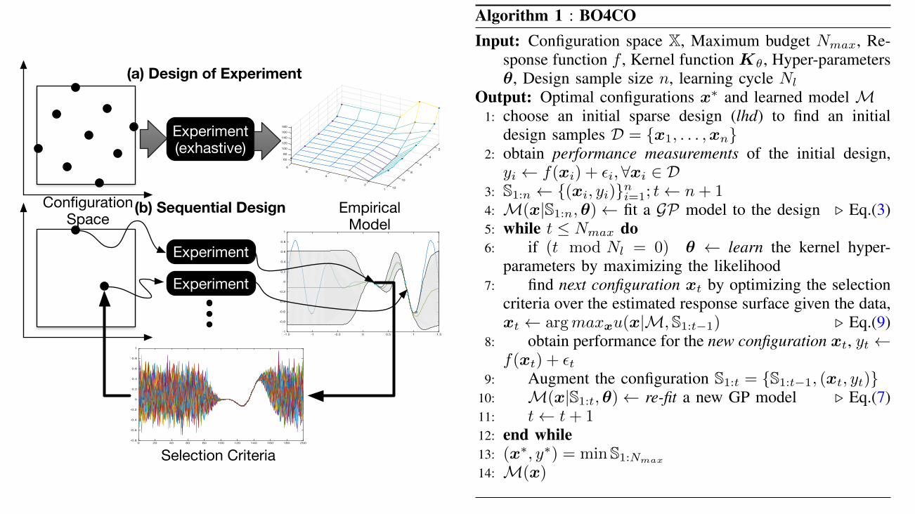
B. BO4CO algorithm

BO4CO’s high-level architecture is shown in Figure 6 andthe procedure that drives the optimization is described in Al-gorithm. We start by bootstrapping the optimization followingLatin Hypercube Design (lhd) to produce an initial designD = {x1, . . . ,xn

} (cf. step 1 in Algorithm 1). Although otherdesign approaches (e.g., random) could be used, we have cho-sen lhd because: (i) it ensures that the configuration samplesin D is representative of the configuration space X, whereastraditional random sampling [17], [9] (called brute-force) doesnot guarantee this [20]; (ii) another advantage is that the lhdsamples can be taken one at a time, making it efficient inhigh dimensional spaces. After obtaining the measurementsregarding the initial design, BO4CO then fits a GP model tothe design points D to form our belief about the underlyingresponse function (cf. step 3 in Algorithm 1). The while loop inAlgorithm 1 iteratively updates the belief until the budget runsout: As we accumulate the data S1:t = {(x

i

, yi

)}ti=1, where

yi

= f(xi

)+ ✏i

with ✏ ⇠ N (0,�2), a prior distribution Pr(f)

and the likelihood function Pr(S1:t|f) form the posteriordistribution: Pr(f |S1:t) / Pr(S1:t|f) Pr(f).

A GP is a distribution over functions [31], specified by itsmean (see Section III-E2), and covariance (see Section III-E1):

y = f(x) ⇠ GP(µ(x), k(x,x0)), (3)

Algorithm 1 : BO4COInput: Configuration space X, Maximum budget N

max

, Re-sponse function f , Kernel function K

✓

, Hyper-parameters✓, Design sample size n, learning cycle N

l

Output: Optimal configurations x

⇤ and learned model M1: choose an initial sparse design (lhd) to find an initial

design samples D = {x1, . . . ,xn

}2: obtain performance measurements of the initial design,

yi

f(xi

) + ✏i

, 8xi

2 D3: S1:n {(x

i

, yi

)}ni=1; t n+ 1

4: M(x|S1:n,✓) fit a GP model to the design . Eq.(3)5: while t N

max

do6: if (t mod N

l

= 0) ✓ learn the kernel hyper-parameters by maximizing the likelihood

7: find next configuration x

t

by optimizing the selectioncriteria over the estimated response surface given the data,x

t

argmaxx

u(x|M, S1:t�1) . Eq.(9)8: obtain performance for the new configuration x

t

, yt

f(x

t

) + ✏t

9: Augment the configuration S1:t = {S1:t�1, (xt

, yt

)}10: M(x|S1:t,✓) re-fit a new GP model . Eq.(7)11: t t+ 1

12: end while13: (x

⇤, y⇤) = min S1:Nmax

14: M(x)

where k(x,x0) defines the distance between x and x

0. Let usassume S1:t = {(x1:t, y1:t)|yi := f(x

i

)} be the collection oft observations. The function values are drawn from a multi-variate Gaussian distribution N (µ,K), where µ := µ(x1:t),

K :=

2

64k(x1,x1) . . . k(x1,xt

)

.... . .

...k(x

t

,x1) . . . k(xt

,xt

)

3

75 (4)

In the while loop in BO4CO, given the observations weaccumulated so far, we intend to fit a new GP model:

f1:tft+1

�⇠ N (µ,

K + �2

I k

k

| k(xt+1,xt+1)

�), (5)

where k(x)

|= [k(x,x1) k(x,x2) . . . k(x,x

t

)] and I

is identity matrix. Given the Eq. (5), the new GP model canbe drawn from this new Gaussian distribution:

Pr(ft+1|S1:t,xt+1) = N (µ

t

(x

t+1),�2t

(x

t+1)), (6)

where

µt

(x) = µ(x) + k(x)

|(K + �2

I)

�1(y � µ) (7)

�2t

(x) = k(x,x) + �2I � k(x)

|(K + �2

I)

�1k(x) (8)

These posterior functions are used to select the next point xt+1

as detailed in Section III-C.

C. Configuration selection criteriaThe selection criteria is defined as u : X ! R that selects

x

t+1 2 X, should f(·) be evaluated next (step 7):

x

t+1 = argmax

x2Xu(x|M, S1:t) (9)

-1.5 -1 -0.5 0 0.5 1 1.5-1

-0.8

-0.6

-0.4

-0.2

0

0.2

0.4

0.6

0.8

1

Configuration Space

Empirical Model

2

4

6

8

10

1212

34

56

160

140

120

100

80

60

180Experiment(exhastive)

Experiment

Experiment

0 20 40 60 80 100 120 140 160 180 200-0.8

-0.6

-0.4

-0.2

0

0.2

0.4

0.6

0.8

1

Selection Criteria

(b) Sequential Design

(a) Design of Experiment

-1.5 -1 -0.5 0 0.5 1 1.5-0.8

-0.6

-0.4

-0.2

0

0.2

0.4

0.6

0.8

configuration domain

resp

onse

val

ue

-1.5 -1 -0.5 0 0.5 1 1.5-0.8

-0.6

-0.4

-0.2

0

0.2

0.4

0.6

0.8

1 true response functionGP fit

-1.5 -1 -0.5 0 0.5 1 1.5-0.8

-0.6

-0.4

-0.2

0

0.2

0.4

0.6

0.8

1

criteria evaluation

new selected point

-1.5 -1 -0.5 0 0.5 1 1.5-0.8

-0.6

-0.4

-0.2

0

0.2

0.4

0.6

0.8

1

new GP fit

Acquisition function:

-1.5 -1 -0.5 0 0.5 1 1.5-1.5

-1

-0.5

0

0.5

1

x1 x2 x3 x4

true function

GP surrogate mean estimate

observation

Fig. 5: An example of 1D GP model: GPs provide mean esti-mates as well as the uncertainty in estimations, i.e., variance.



Monitoring

Deployment Service

Data Preparation


values


values

Experimental Suite

Testbed

Doc

Data Broker

Tester



GP model

Kafka



Stor

m

Cas

sand

ra

Spar

k

Fig. 6: BO4CO architecture: (i) optimization and (ii) exper-imental suite are integrated via (iii) a data broker. The in-tegrated solution is available: https://github.com/dice-project/DICE-Configuration-BO4CO.

B. BO4CO algorithm

BO4CO’s high-level architecture is shown in Figure 6 andthe procedure that drives the optimization is described in Al-gorithm. We start by bootstrapping the optimization followingLatin Hypercube Design (lhd) to produce an initial designD = {x1, . . . ,xn

} (cf. step 1 in Algorithm 1). Although otherdesign approaches (e.g., random) could be used, we have cho-sen lhd because: (i) it ensures that the configuration samplesin D is representative of the configuration space X, whereastraditional random sampling [22], [11] (called brute-force)does not guarantee this [25]; (ii) another advantage is thatthe lhd samples can be taken one at a time, making it efficientin high dimensional spaces. After obtaining the measurementsregarding the initial design, BO4CO then fits a GP model tothe design points D to form our belief about the underlyingresponse function (cf. step 3 in Algorithm 1). The while loop inAlgorithm 1 iteratively updates the belief until the budget runsout: As we accumulate the data S1:t = {(x

i

, yi

)}ti=1, where

yi

= f(xi

)+ ✏i

with ✏ ⇠ N (0,�2), a prior distribution Pr(f)

and the likelihood function Pr(S1:t|f) form the posteriordistribution: Pr(f |S1:t) / Pr(S1:t|f) Pr(f).

A GP is a distribution over functions [37], specified by itsmean (see Section III-E2), and covariance (see Section III-E1):

y = f(x) ⇠ GP(µ(x), k(x,x0)), (3)

Algorithm 1 : BO4COInput: Configuration space X, Maximum budget N

max

, Re-sponse function f , Kernel function K

✓

, Hyper-parameters✓, Design sample size n, learning cycle N

l

Output: Optimal configurations x

⇤ and learned model M1: choose an initial sparse design (lhd) to find an initial

design samples D = {x1, . . . ,xn

}2: obtain performance measurements of the initial design,

yi

f(xi

) + ✏i

, 8xi

2 D3: S1:n {(x

i

, yi

)}ni=1; t n+ 1

4: M(x|S1:n,✓) fit a GP model to the design . Eq.(3)5: while t N

max

do6: if (t mod N

l

= 0) ✓ learn the kernel hyper-parameters by maximizing the likelihood

7: find next configuration x

t

by optimizing the selectioncriteria over the estimated response surface given the data,x

t

argmaxx

u(x|M, S1:t�1) . Eq.(9)8: obtain performance for the new configuration x

t

, yt

f(x

t

) + ✏t

9: Augment the configuration S1:t = {S1:t�1, (xt

, yt

)}10: M(x|S1:t,✓) re-fit a new GP model . Eq.(7)11: t t+ 1

12: end while13: (x

⇤, y⇤) = min S1:Nmax

14: M(x)

where k(x,x0) defines the distance between x and x

0. Let usassume S1:t = {(x1:t, y1:t)|yi := f(x

i

)} be the collection oft observations. The function values are drawn from a multi-variate Gaussian distribution N (µ,K), where µ := µ(x1:t),

K :=

2

64k(x1,x1) . . . k(x1,xt

)

.... . .

...k(x

t

,x1) . . . k(xt

,xt

)

3

75 (4)

In the while loop in BO4CO, given the observations weaccumulated so far, we intend to fit a new GP model:

f1:tft+1

�⇠ N (µ,

K + �2

I k

k

| k(xt+1,xt+1)

�), (5)

where k(x)

|= [k(x,x1) k(x,x2) . . . k(x,x

t

)] and I

is identity matrix. Given the Eq. (5), the new GP model canbe drawn from this new Gaussian distribution:

Pr(ft+1|S1:t,xt+1) = N (µ

t

(x

t+1),�2t

(x

t+1)), (6)

where

µt

(x) = µ(x) + k(x)

|(K + �2

I)

�1(y � µ) (7)

�2t

(x) = k(x,x) + �2I � k(x)

|(K + �2

I)

�1k(x) (8)

These posterior functions are used to select the next point xt+1

as detailed in Section III-C.

C. Configuration selection criteriaThe selection criteria is defined as u : X ! R that selects

x

t+1 2 X, should f(·) be evaluated next (step 7):

x

t+1 = argmax

x2Xu(x|M, S1:t) (9)

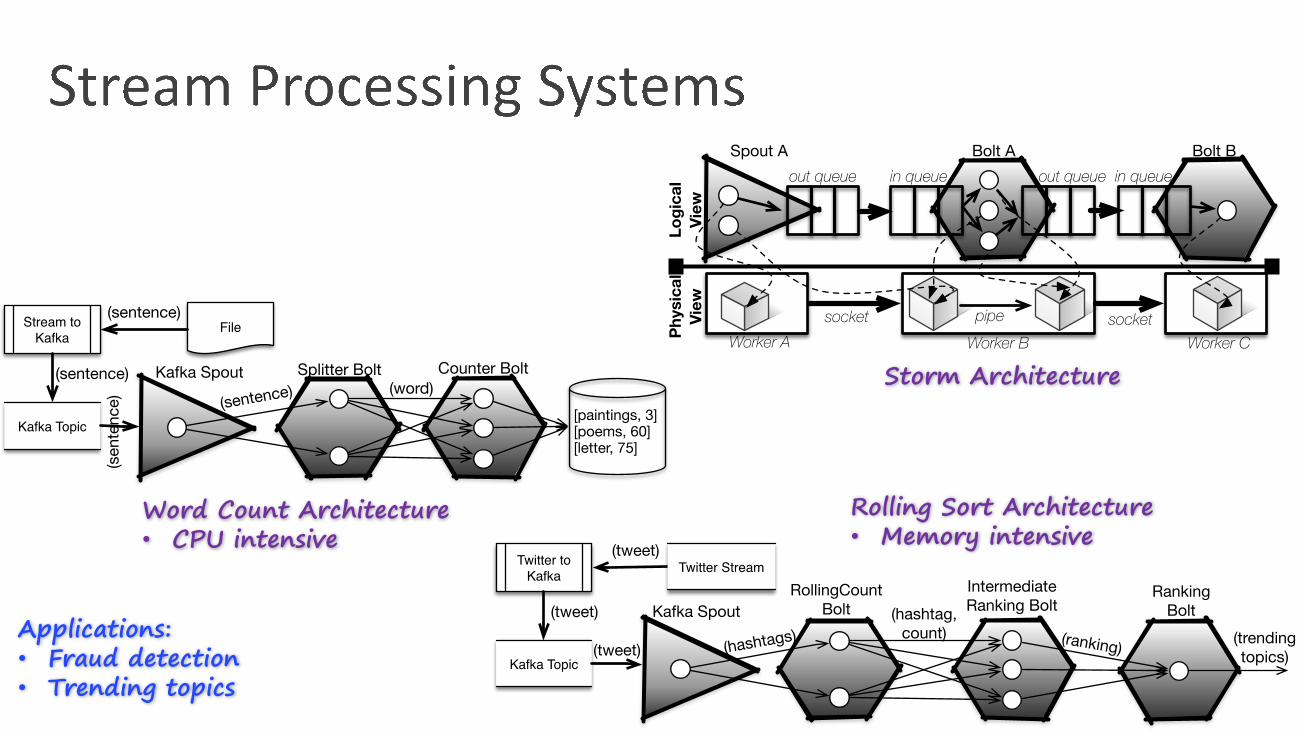
Logi

cal

View

Phys

ical

Vi

ew pipe

Spout A Bolt A Bolt B

socket socket

out queue in queue

Worker A Worker B Worker C

out queue in queue



Kafka Topic

Stream to Kafka

File(sentence)

(sentence)

(sen

tenc

e)

Kafka SpoutRollingCount

BoltIntermediateRanking Bolt

(hashtags)(hashtag,

count)

Ranking Bolt

(ranking) (trending topics)Kafka Topic

Twitter to Kafka

(tweet)Twitter Stream

(tweet)

(tweet)

Storm Architecture

Word Count Architecture• CPU intensive

Rolling Sort Architecture• Memory intensive

Applications:• Fraud detection• Trending topics

Experimentalresults

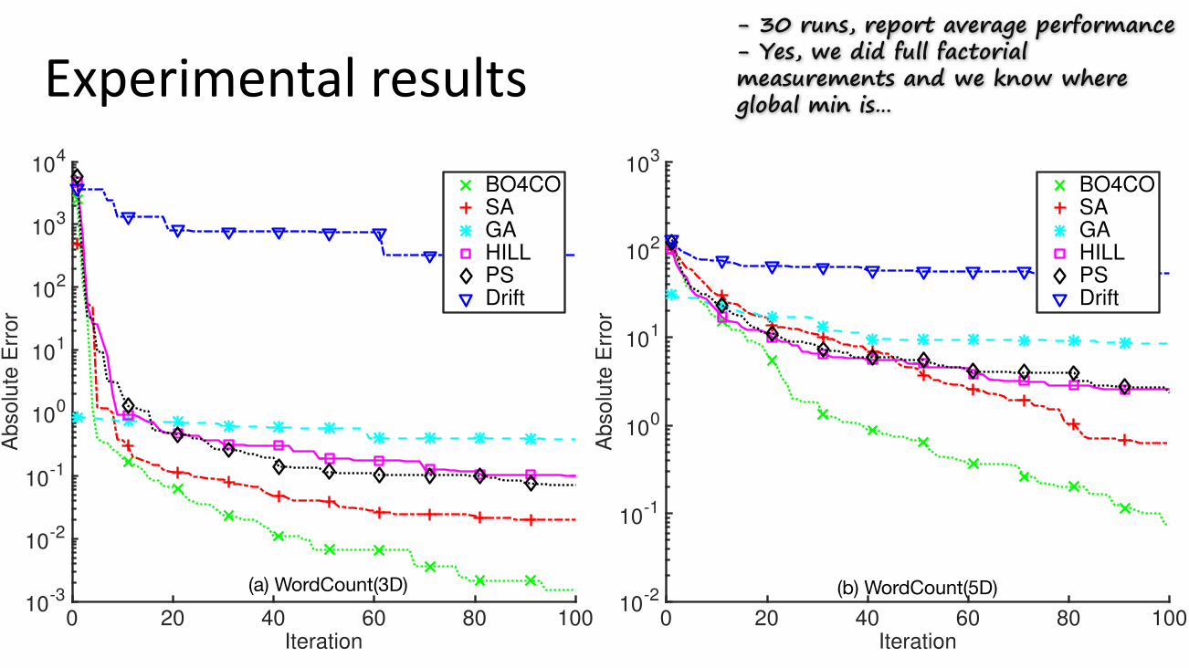
0 20 40 60 80 100

Iteration

10-3

10-2

10-1

100

101

102

103

104

Ab

solu

te E

rro

r

BO4CO

SA

GA

HILL

PS

Drift

0 20 40 60 80 100

Iteration

10-2

10-1

100

101

102

103

Ab

solu

te E

rro

r

BO4CO

SA

GA

HILL

PS

Drift

(a) WordCount(3D) (b) WordCount(5D)

- 30 runs, report average performance- Yes, we did full factorial measurements and we know where global min is…

Experimentalresults

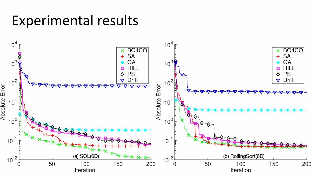
0 50 100 150 200

Iteration

10-2

10-1

100

101

102

103

104

Ab

so

lute

Err

or

BO4CO

SA

GA

HILL

PS

Drift

0 50 100 150 200

Iteration

10-2

10-1

100

101

102

103

104

Ab

so

lute

Err

or

BO4CO

SA

GA

HILL

PS

Drift

(a) SOL(6D) (b) RollingSort(6D)

Experimentalresults

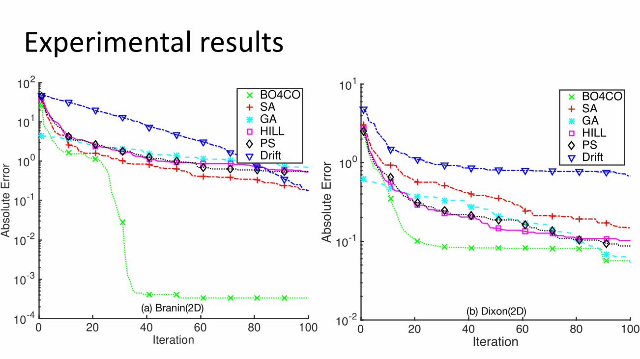
0 20 40 60 80 100

Iteration

10-4

10-3

10-2

10-1

100

101

102

Absolu

te E

rror

BO4CO

SA

GA

HILL

PS

Drift

0 20 40 60 80 100Iteration

10-2

10-1

100

101

Abso

lute

Erro

r

BO4COSAGAHILLPSDrift

(a) Branin(2D) (b) Dixon(2D)

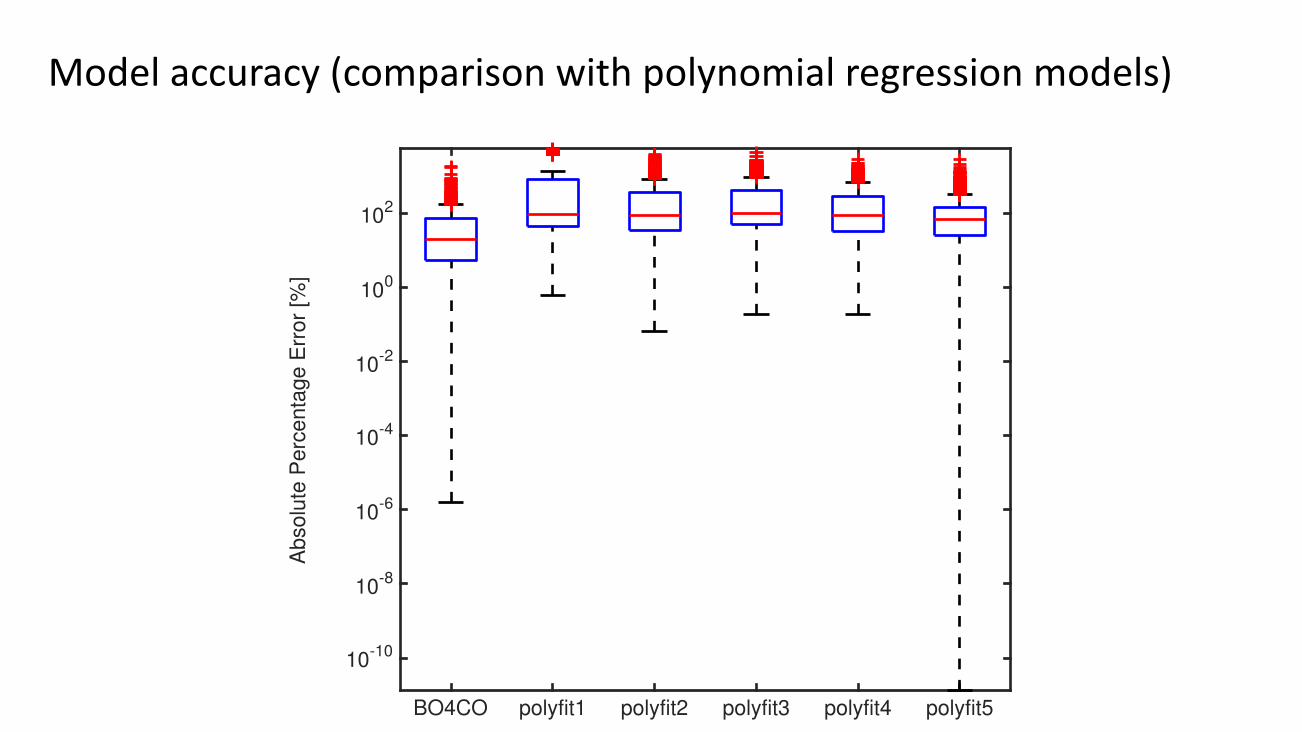
Modelaccuracy(comparisonwithpolynomialregressionmodels)

BO4CO polyfit1 polyfit2 polyfit3 polyfit4 polyfit5

10-10

10-8

10-6

10-4

10-2

100

102

Abso

lute

Perc

enta

ge E

rror

[%]

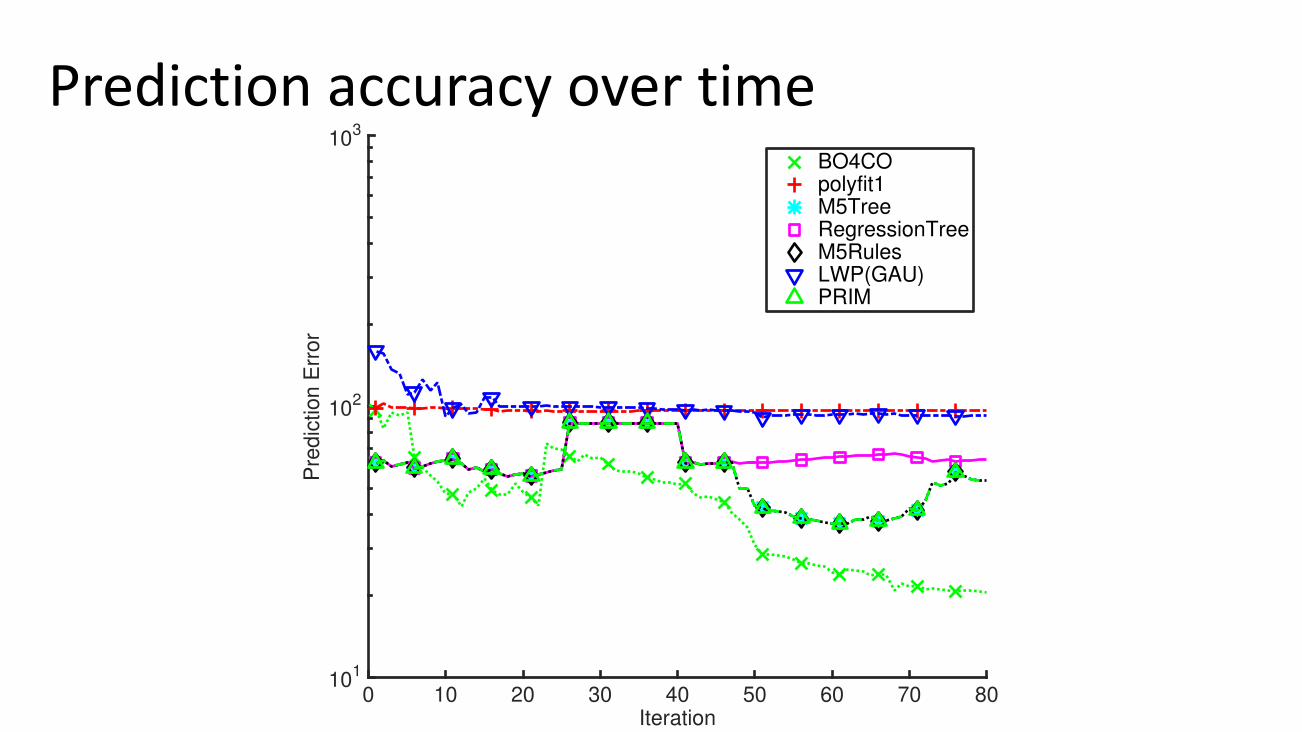
Predictionaccuracyovertime

0 10 20 30 40 50 60 70 80Iteration

101

102

103

Pre

dic

tion E

rror

BO4COpolyfit1M5TreeRegressionTreeM5RulesLWP(GAU)PRIM

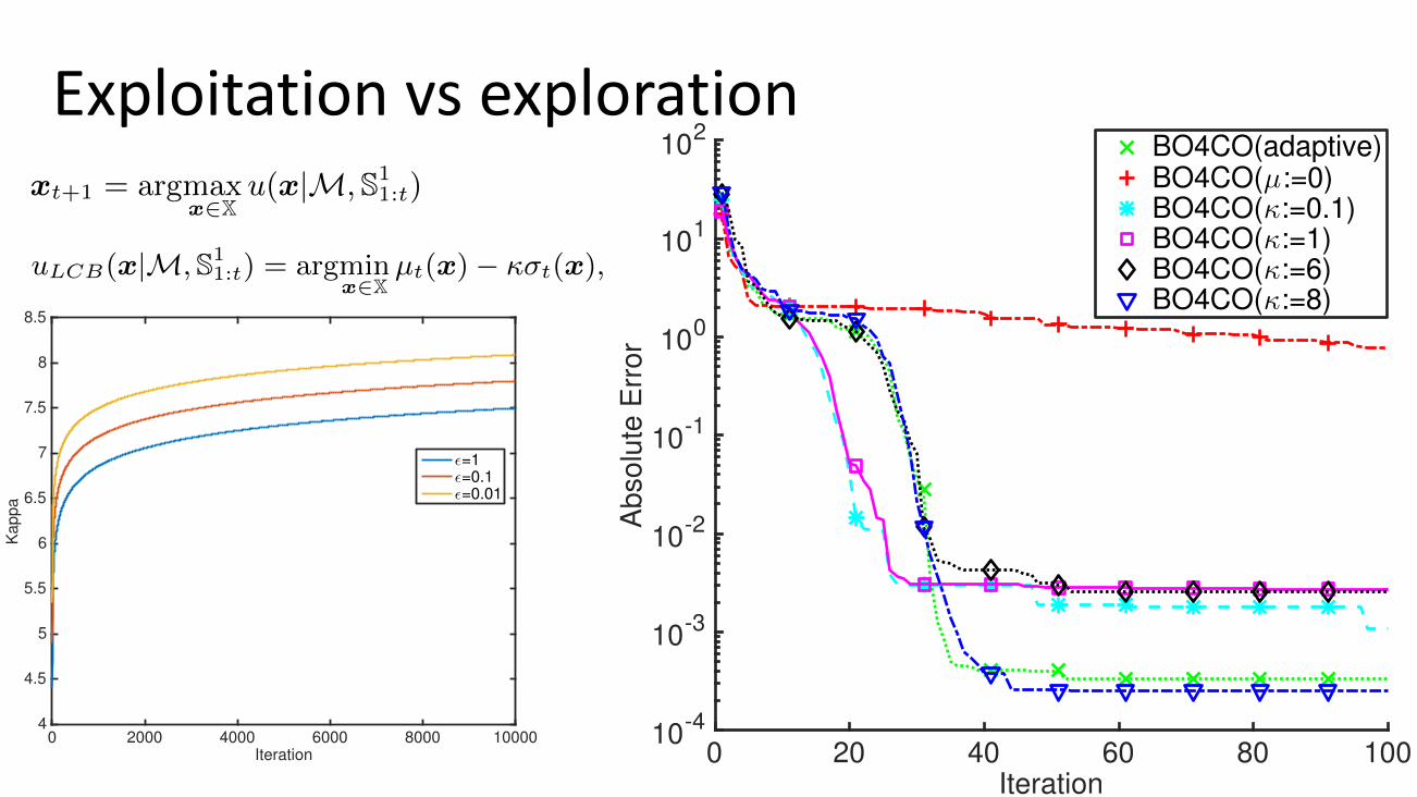
Exploitationvsexploration

0 20 40 60 80 100Iteration

10-4

10-3

10-2

10-1

100

101

102

Abso

lute

Err

or

BO4CO(adaptive)BO4CO(µ:=0)BO4CO(κ:=0.1)BO4CO(κ:=1)BO4CO(κ:=6)BO4CO(κ:=8)

0 2000 4000 6000 8000 10000Iteration

4

4.5

5

5.5

6

6.5

7

7.5

8

8.5

Ka

pp

a

ϵ=1ϵ=0.1ϵ=0.01

Figure 5. Three di↵erent 1D (1-dimensional) response func-tions are to be minimized. Further samples are available allover two of them, whereas function (1) that is under test hasonly few sparse observations. Merely using these few sampleswould result in poor (uninformative) predictions of the func-tion especially in the areas where there is no observations.Using the correlation with the other two functions enablesthe MTGP model to provide more accurate predictions andas a result locating the optimum more quickly.

3.3 Filtering out irrelevant dataHere is described how the selection of the points in the

previous system is made. The number of historical observa-tions taken in consideration is important because a↵ect thecomputational requirements, due to the matrix inversion in(6) incurs a cubic cost (shown in Section 4.6). TL4CO selects(step 3 in Algorithm 1) points with the lowest entropy value.Entropy reduction is computed as the log of the ratio of theposterior uncertainty given an observation xi,j belonging toversion j, to its uncertainty without it:

Iij = log⇣v(x|X,xi,j)

v(x|X)

⌘, (8)

where v(x|X) is the posterior uncertainty of the predictionfrom MTGP model of query point x obtained in (7).

3.4 Model fitting in TL4COIn this section, we provide some practical considerations

and the extensions we made to the MTGP framework tomake it applicable for configuration optimization.

3.4.1 Kernel functionWe implemented the following kernel function to support

integer and categorical variables (cf. Section 2.1):

kxx(xi,xj) = exp(⌃d`=1(�✓`�(xi 6= xj))), (9)

where d is the number of dimensions (i.e., the number ofconfiguration parameters), ✓` adjust the scales along thefunction dimensions and � is a function gives the distancebetween two categorical variables using Kronecker delta [20,34]. TL4CO uses di↵erent scales {✓`, ` = 1 . . . d} on di↵erentdimensions as suggested in [41, 34], this technique is calledAutomatic Relevance Determination (ARD). After learningthe hyper-parameters (step 7 in Algorithm 1), if the `-thdimension (parameter) turns out be irrelevant, so the ✓`will be a small value, and therefore, will be automaticallydiscarded. This is particularly helpful in high dimensionalspaces, where it is di�cult to find the optimal configuration.

3.4.2 Prior mean functionWhile the kernel controls the structure of the estimated

function, the prior mean µ(x) : X ! R provides a possibleo↵set for our estimation. By default, this function is set to aconstant µ(x) := µ, which is inferred from the observations[34]. However, the prior mean function is a way of incorpo-rating the expert knowledge, if it is available, then we canuse this knowledge. Fortunately, we have collected extensiveexperimental measurements and based on our datasets (cf.Table 3), we observed that typically, for Big Data systems,there is a significant distance between the minimum and themaximum of each function (cf. Figure 2). Therefore, a linearmean function µ(x) := ax+ b, allows for more flexible struc-tures, and provides a better fit for the data than a constantmean. We only need to learn the slope for each dimensionand an o↵set (denoted by µ` = (a, b), see next).

3.4.3 Learning hyper-parametersThis section describe the step 7 in Algorithm 1. Due to the

heavy computation of the learning, this process is computedonly every Nl iterations. For learning the hyper-parametersof the kernel and also the prior mean functions (cf. Sections3.4.1 and 3.4.2), we maximize the marginal likelihood [34,5] of the observations S1

1:t. To do that, we train our GPmodel (6) with S1

1:t . We optimize the marginal likelihoodusing multi-started quasi-Newton hill-climbers [32]. For thispurpose, we use the o↵-the-shelf gpml library presented in[32]. Using the multi-task kernel defined in (5), we learn✓ := (✓t, ✓xx, µ`) that comprises the hyper-parameters of kt,kxx (cf. (5)) and the mean function µ(·) (cf. Section 3.4.2).The learning is performed iteratively resulting in a sequenceof priors with parameters ✓i for i = 1 . . . bN

max

N`

c.

3.4.4 Observation noiseIn Section 2.4, we have shown that such noise level can

be measured with a high confidence and the signal-to-noiseratios shows that such noise is stationary. In (7), � representsthe noise of the selected point x. Typically this noise valueis not known. In TL4CO, we estimate the noise level by anapproximation. The query points can be assumed to be asnoisy as the observed data. In other words, we treat � as arandom variable and we calculate its expected value as:

� =⌃T

j=1Ni�2i

⌃Ti=1Ni

(10)

where Ni are the number of observations from the ith datasetand �2

i is the noise variance of the individual datasets.

3.5 Configuration selection criteriaTL4CO requires a selection criterion (step 8 in Algorithm

1) to decide the next configuration to measure. Intuitively,we want to select the minimum response. This is done usinga utility function u : X ! R that determines xt+1 2 X,should f(·) be evaluated next as:

xt+1 = argmaxx2X

u(x|M, S11:t) (11)

The selection criterion depends on the MTGP model Msolely through its predictive mean µt(xt) and variance �2

t (xt)conditioned on observations S1

1:t. TL4CO uses the LowerConfidence Bound (LCB) [24]:

uLCB(x|M, S11:t) = argmin

x2Xµt(x)� �t(x), (12)

where is a exploitation-exploration parameter. For instance,if we require to find a near optimal configuration we set alow value to to take the most out of the predictive mean.However, if we are looking for a globally optimum one, we canset a high value in order to skip local minima. Furthermore, can be adapted over time [22] to perform more explorations.Figure 6 shows that in TL4CO, can start with a relativelyhigher value at the early iterations comparing to BO4COsince the former provides a better estimate of mean andtherefore contains more information at the early stages.

TL4CO output. Once the Nmax di↵erent configurations ofthe system under test are measured, the TL4CO algorithmterminates. Finally, TL4CO produces the outputs includingthe optimal configuration (step 14 in Algorithm 1) as wellas the learned MTGP model (step 15 in Algorithm 1). Allthese information are versioned and stored in a performancerepository (cf. Figure 7) to be used in the future versions ofthe system.

5

Figure 5. Three di↵erent 1D (1-dimensional) response func-tions are to be minimized. Further samples are available allover two of them, whereas function (1) that is under test hasonly few sparse observations. Merely using these few sampleswould result in poor (uninformative) predictions of the func-tion especially in the areas where there is no observations.Using the correlation with the other two functions enablesthe MTGP model to provide more accurate predictions andas a result locating the optimum more quickly.

3.3 Filtering out irrelevant dataHere is described how the selection of the points in the

previous system is made. The number of historical observa-tions taken in consideration is important because a↵ect thecomputational requirements, due to the matrix inversion in(6) incurs a cubic cost (shown in Section 4.6). TL4CO selects(step 3 in Algorithm 1) points with the lowest entropy value.Entropy reduction is computed as the log of the ratio of theposterior uncertainty given an observation xi,j belonging toversion j, to its uncertainty without it:

Iij = log⇣v(x|X,xi,j)

v(x|X)

⌘, (8)

where v(x|X) is the posterior uncertainty of the predictionfrom MTGP model of query point x obtained in (7).

3.4 Model fitting in TL4COIn this section, we provide some practical considerations

and the extensions we made to the MTGP framework tomake it applicable for configuration optimization.

3.4.1 Kernel functionWe implemented the following kernel function to support

integer and categorical variables (cf. Section 2.1):

kxx(xi,xj) = exp(⌃d`=1(�✓`�(xi 6= xj))), (9)

where d is the number of dimensions (i.e., the number ofconfiguration parameters), ✓` adjust the scales along thefunction dimensions and � is a function gives the distancebetween two categorical variables using Kronecker delta [20,34]. TL4CO uses di↵erent scales {✓`, ` = 1 . . . d} on di↵erentdimensions as suggested in [41, 34], this technique is calledAutomatic Relevance Determination (ARD). After learningthe hyper-parameters (step 7 in Algorithm 1), if the `-thdimension (parameter) turns out be irrelevant, so the ✓`will be a small value, and therefore, will be automaticallydiscarded. This is particularly helpful in high dimensionalspaces, where it is di�cult to find the optimal configuration.

3.4.2 Prior mean functionWhile the kernel controls the structure of the estimated

function, the prior mean µ(x) : X ! R provides a possibleo↵set for our estimation. By default, this function is set to aconstant µ(x) := µ, which is inferred from the observations[34]. However, the prior mean function is a way of incorpo-rating the expert knowledge, if it is available, then we canuse this knowledge. Fortunately, we have collected extensiveexperimental measurements and based on our datasets (cf.Table 3), we observed that typically, for Big Data systems,there is a significant distance between the minimum and themaximum of each function (cf. Figure 2). Therefore, a linearmean function µ(x) := ax+ b, allows for more flexible struc-tures, and provides a better fit for the data than a constantmean. We only need to learn the slope for each dimensionand an o↵set (denoted by µ` = (a, b), see next).

3.4.3 Learning hyper-parametersThis section describe the step 7 in Algorithm 1. Due to the

heavy computation of the learning, this process is computedonly every Nl iterations. For learning the hyper-parametersof the kernel and also the prior mean functions (cf. Sections3.4.1 and 3.4.2), we maximize the marginal likelihood [34,5] of the observations S1

1:t. To do that, we train our GPmodel (6) with S1

1:t . We optimize the marginal likelihoodusing multi-started quasi-Newton hill-climbers [32]. For thispurpose, we use the o↵-the-shelf gpml library presented in[32]. Using the multi-task kernel defined in (5), we learn✓ := (✓t, ✓xx, µ`) that comprises the hyper-parameters of kt,kxx (cf. (5)) and the mean function µ(·) (cf. Section 3.4.2).The learning is performed iteratively resulting in a sequenceof priors with parameters ✓i for i = 1 . . . bN

max

N`

c.

3.4.4 Observation noiseIn Section 2.4, we have shown that such noise level can

be measured with a high confidence and the signal-to-noiseratios shows that such noise is stationary. In (7), � representsthe noise of the selected point x. Typically this noise valueis not known. In TL4CO, we estimate the noise level by anapproximation. The query points can be assumed to be asnoisy as the observed data. In other words, we treat � as arandom variable and we calculate its expected value as:

� =⌃T

j=1Ni�2i

⌃Ti=1Ni

(10)

where Ni are the number of observations from the ith datasetand �2

i is the noise variance of the individual datasets.

3.5 Configuration selection criteriaTL4CO requires a selection criterion (step 8 in Algorithm

1) to decide the next configuration to measure. Intuitively,we want to select the minimum response. This is done usinga utility function u : X ! R that determines xt+1 2 X,should f(·) be evaluated next as:

xt+1 = argmaxx2X

u(x|M, S11:t) (11)

The selection criterion depends on the MTGP model Msolely through its predictive mean µt(xt) and variance �2

t (xt)conditioned on observations S1

1:t. TL4CO uses the LowerConfidence Bound (LCB) [24]:

uLCB(x|M, S11:t) = argmin

x2Xµt(x)� �t(x), (12)

where is a exploitation-exploration parameter. For instance,if we require to find a near optimal configuration we set alow value to to take the most out of the predictive mean.However, if we are looking for a globally optimum one, we canset a high value in order to skip local minima. Furthermore, can be adapted over time [22] to perform more explorations.Figure 6 shows that in TL4CO, can start with a relativelyhigher value at the early iterations comparing to BO4COsince the former provides a better estimate of mean andtherefore contains more information at the early stages.

TL4CO output. Once the Nmax di↵erent configurations ofthe system under test are measured, the TL4CO algorithmterminates. Finally, TL4CO produces the outputs includingthe optimal configuration (step 14 in Algorithm 1) as wellas the learned MTGP model (step 15 in Algorithm 1). Allthese information are versioned and stored in a performancerepository (cf. Figure 7) to be used in the future versions ofthe system.

5

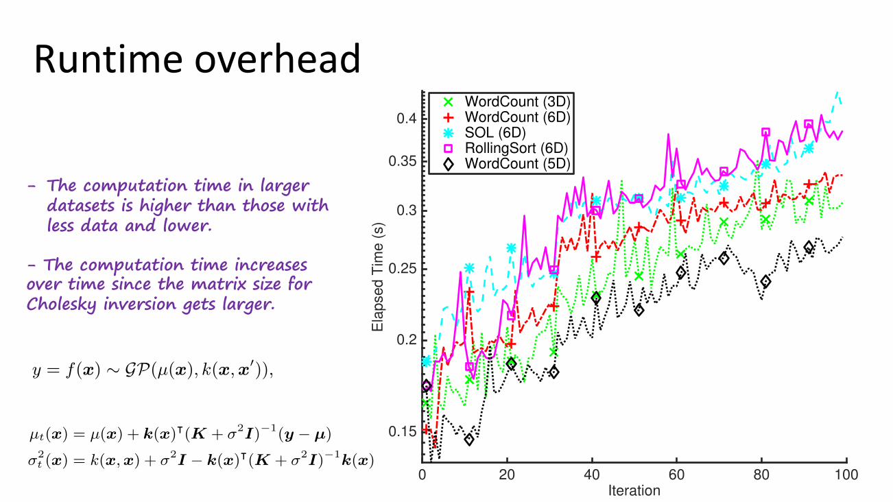
Runtimeoverhead

0 20 40 60 80 100Iteration

0.15

0.2

0.25

0.3

0.35

0.4

Ela

pse

d T

ime (

s)

WordCount (3D)WordCount (6D)SOL (6D)RollingSort (6D)WordCount (5D)

- The computation time in larger datasets is higher than those with less data and lower.

- The computation time increases over time since the matrix size for Cholesky inversion gets larger.


v1 1 0.41 (0.49) -0.46 (-0.51) -0.50 (-0.51)v2 7.36E-06 (5.5E-08) 1 -0.20 (-0.2793) -0.18 (-0.24)v3 6.92E-07 (1.3E-08) 0.04 (0.003) 1 0.94 (0.88)v4 2.54E-08 (1.4E-08) 0.07 (0.01) 1.16E-52 (8.3E-36) 1



wc(v1) 516.59 7.96 [515.27, 517.90] [7.13, 9.01] 64.88wc(v2) 584.94 2.58 [584.51, 585.36] [2.32, 2.92] 226.32wc(v3) 654.89 13.56 [652.65, 657.13] [12.15, 15.34] 48.30wc(v4) 1125.81 16.92 [1123, 1128.6] [15.16, 19.14] 66.56



v2 = (6, 2), x⇤v3 = (2, 13), x⇤








y = f(x) ⇠ GP(µ(x), k(x,x0)), (2)


and x


µt(x) = µ(x) + k(x)|(K + �2I)�1(y � µ) (3)

�2t (x) = k(x,x) + �2

I � k(x)|(K + �2I)�1

k(x) (4)






3


v1 1 0.41 (0.49) -0.46 (-0.51) -0.50 (-0.51)v2 7.36E-06 (5.5E-08) 1 -0.20 (-0.2793) -0.18 (-0.24)v3 6.92E-07 (1.3E-08) 0.04 (0.003) 1 0.94 (0.88)v4 2.54E-08 (1.4E-08) 0.07 (0.01) 1.16E-52 (8.3E-36) 1



wc(v1) 516.59 7.96 [515.27, 517.90] [7.13, 9.01] 64.88wc(v2) 584.94 2.58 [584.51, 585.36] [2.32, 2.92] 226.32wc(v3) 654.89 13.56 [652.65, 657.13] [12.15, 15.34] 48.30wc(v4) 1125.81 16.92 [1123, 1128.6] [15.16, 19.14] 66.56



v2 = (6, 2), x⇤v3 = (2, 13), x⇤








y = f(x) ⇠ GP(µ(x), k(x,x0)), (2)


and x


µt(x) = µ(x) + k(x)|(K + �2I)�1(y � µ) (3)

�2t (x) = k(x,x) + �2

I � k(x)|(K + �2I)�1

k(x) (4)






3

Keytakeaways

- Aprincipledwayfor- locating optimal configurations - carefully choosing where to sample - by sequentially reducing uncertainty in the response surface- in order to reduce the number of measurements

- GPs appearedtobemoreaccuratethanothermachinelearningregressionmodelsinourexperiments.

- ApplicationstoSPSs,Batch andNoSQL (seetheBO4COgithub pageformoredetails)

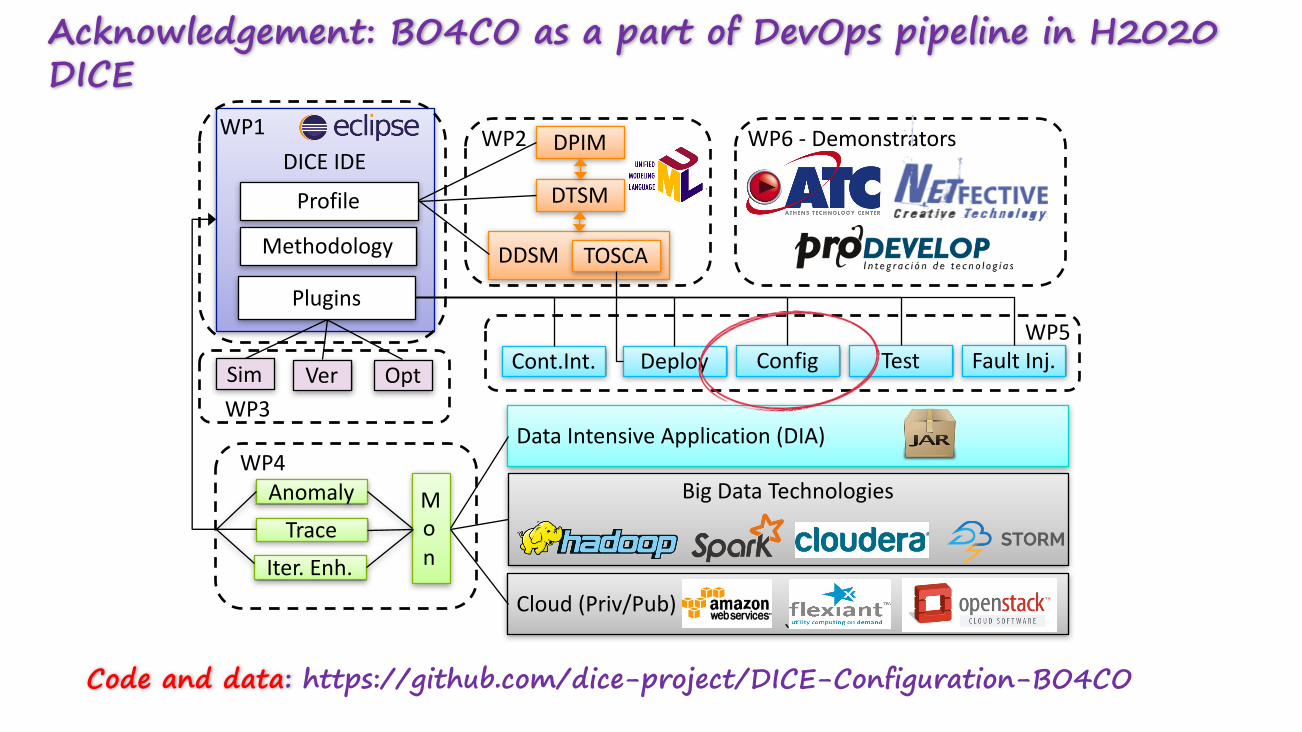
Acknowledgement: BO4CO as a part of DevOps pipeline in H2020 DICE

BigDataTechnologies

Cloud(Priv/Pub)`

DICEIDE

Profile

Plugins

Sim Ver Opt

DPIM

DTSM

DDSMTOSCAMethodology

Deploy Config Test

Mon

AnomalyTrace

Iter.Enh.

DataIntensiveApplication(DIA)

Cont.Int. FaultInj.

WP4

WP3

WP2

WP5

WP1 WP6- Demonstrators

Code and data: https://github.com/dice-project/DICE-Configuration-BO4CO