Contents lists available at ScienceDirect

Ultrasonics - Sonochemistry

journal homepage: www.elsevier.com/locate/ultson

Numerical modelling of acoustic pressure fields to optimize the ultrasoniccleaning technique for cylinders

Habiba Laisa,b,⁎, Premesh S. Lowea, Tat-Hean Gana, Luiz C. Wrobelb

a Brunel Innovation Centre, Granta Park, Great Abington, Cambridge CB21 6AL, UKb Brunel University, Kingston Lane, Uxbridge, Middlesex UB8 3PH, UK

A R T I C L E I N F O

Keywords:CavitationCOMSOLExcitationFouling removalNumerical modellingUltrasonic transducers

A B S T R A C T

Fouling build up is a well-known problem in the offshore industry. Accumulation of fouling occurs in differentstructures, e.g. offshore pipes, ship hulls, floating production platforms. The type of fouling that accumulates isdependent on environmental conditions surrounding the structure itself. Current methods deployed for foulingremoval span across hydraulic, chemical and manual, all sharing the common disadvantage of necessitatinghalting production for the cleaning process to commence. Conventionally, ultrasound is used in ultrasonic bathsto clean a submerged component by the generation and implosion of cavitation bubbles on the fouled surface;this method is particularly used in Reverse Osmosis applications. However, this requires the submersion of thefouled structure and thus may require a halt to production. Large fouled structures such as pipelines may not beaccommodated. The application of high power ultrasonics is proposed in this work as a means to remove foulingon a structure whilst in operation. The work presented in this paper consists of the development of a finiteelement analysis model based on successful cleaning results from a pipe fouled with calcite on the inner pipewall. A Polytec 3D Laser Doppler Vibrometer was used in this investigation to study the fouling removal process.Results show the potential of high power ultrasonics for fouling removal in pipe structures from the wavepropagation across the structure under excitation, and are used to validate a COMSOL model to determinecleaning patterns based on pressure and displacement distributions for future transducer array design and op-timization.

1. Introduction

Fouling formation is a major problem for the offshore industry [1].It is an important factor contributing to the assessment of service life-time and safety of marine facilities [2]. Consequently, large sums ofmoney are spent in cleaning and preventative measures to maintainoffshore structures in a state of operation and efficiency. Currentmethods deployed for fouling removal include hydraulic, chemical andmanual, having a common disadvantage – in that it is mandatory to haltthe operation of the structure in order to commence the fouling removalprocess. Most common fouling mechanisms in offshore structures are;deposition of hard scale and the settlement and growth of marine or-ganisms. This accumulation of fouling can occur in different en-gineering structures such as pipes and ship hulls. The type of foulingthat can be accumulated is dependent on environmental conditionssurrounding the structure itself.

Scaling occurs when saturated brine undergoes a temperature orpressure change causing the solubility to decrease, which results in theprecipitation of solid crystals. The Calcium Carbonate (calcite)

composition in pipelines is an example of the most common scalingproblem in offshore structures. Other common scales that form in off-shore process lines are Barium Sulphate (barite), Strontium Sulphateand Magnesium Sulphate [3]. Sometimes scaling can develop rapidlycausing complete pipe blockage within 24 h [4]. On a slower timescale,biofouling is the growth of marine organisms. This includes algae,micro and macro organisms [5]. On complex and large offshore struc-tures, fouling may be insignificant in relation to the structure’s weightbut fouling on the internal surface of the pipe is a significant problemwhen it causes blockages, rupture and damages to the structure.

The current removal methods deployed in industry can be costlyand time consuming due to halts in production. A successful method offouling removal is the use of chemicals [6] as this achieves up to 100%de-fouling but with the downside of negative environmental impact dueto the release of chemicals after use, as well as down-time of the facility.Another promising method of fouling removal that has recently sur-faced is the use of ultrasound. Currently, ultrasonic baths are used forcleaning individual parts of the offshore plant by generating cavitationbubbles which implode on the fouled surface [7,8], particularly in

https://doi.org/10.1016/j.ultsonch.2018.02.045Received 1 October 2017; Received in revised form 9 February 2018; Accepted 26 February 2018

⁎ Corresponding author at: Brunel Innovation Centre, Granta Park, Great Abington, Cambridge CB21 6AL, UK.E-mail addresses: habiba.lais@brunel.ac.uk (H. Lais), Tat-Hean.Gan@brunel.ac.uk, BIC@brunel.ac.uk (T.-H. Gan).

Ultrasonics - Sonochemistry 45 (2018) 7–16

Available online 03 March 20181350-4177/ © 2018 Elsevier B.V. All rights reserved.

T

Reverse Osmosis applications [9–11]. Conventionally, components thathave accumulated fouling are submerged into an ultrasonic bath whichyet again, requires stopping operation of the structure for the foulingremoval process to commence.

The present paper investigates the potential of using High PowerUltrasonic Transducers (HPUT) to mimic the environmental conditionof an ultrasonic bath in the pipe structures under investigation. Theinvestigation is applied to a Stainless Steel 315 L pipe which is 300mmin length, 1.5 mm in wall thickness and 50.08mm in outer diameterwith a thin layer of Calcite on the inner pipe wall. The paper is orga-nized as follows. Theoretical background is given in Section 2 whileSection 3 consists of the laboratory experimental setup followed by theFinite Element Analysis (FEA) in Section 4. Experimental and numericalresults are discussed in Section 5 followed by discussions in Section 6,conclusions in Section 7 and finally, further work is suggested inSection 8.

2. Theoretical background

2.1. Ultrasonic cavitation

The fouling removal mechanism for the technique discussed in thiswork is by the development and implosion of acoustic cavitation bub-bles. Acoustic cavitation can be defined as the formation of vapourbubbles due to a sudden decrease in pressure in a liquid caused by a(de-)compressional wave [12]. A rarefaction instant is thereby in-troduced and forms a vacuum, where a bubble can appear as shown inFig. 1. During the oscillation of the bubble, the radius increases in therarefaction instants and decreases in the compressional instants. In oneof these cycles, the compression can burst the bubble (adiabatically) toproduce pressures of up to 500 Bar and temperatures up to 5000 K.

There are two types of cavitation bubbles that can form within aliquid; stable cavitation where the bubbles oscillate for a long period oftime in a sound field with a large number of cycles, and transient ca-vitation which lasts for less than one cycle and is violent enough topotentially damage the surface of the body in contact with the liquid[12]. Fig. 1 [13] illustrates and compares the development of stable andtransient cavitation bubbles.

Due to stable cavitation bubbles oscillating for a period of time, theydo not produce any light emission or chemical reactions when im-ploding. However, transient cavitation bubbles implode with a strongcollapse, creating light emissions and/or chemical reactions within theliquid as a result of the implosion [14].

Although two types of cavitation have been defined, cavitation

bubbles can also be a combination of both stable and transient cavita-tion, as discussed in the literature by Yasui in 2018 [14]. This phe-nomenon is also known as ‘high energy stable’ and ‘repetitive transientcavitation’. Cavitation bubbles that are a combination of both types ofcavitation oscillate for a long period of time similarly to stable cavita-tion however, they produce small amounts of light emission and che-mical reactions. An example of this combination of both stable andtransient cavitation can be found in Single-Bubble Sonoluminescence(SBSL) [15].

Stable cavitation oscillates at the excitation frequency of thetransducer as well as the harmonics and subharmonics of the cavitation[16]. These harmonics and subharmonics produce acoustic emissionwhich can be detected to indicate the generation of the cavitation. Thenon-linear nature of a single spherical oscillating cavitation bubble isexplained by the Rayleigh-Plesset equation [17]:

−= + ⎛

⎝⎞⎠

+ +∞p t p tρ

R d Rdt

dRdt

νR

dRdt

sρ R

( ) ( ) 32

4 2

L

L

L

2

2

2

(1)

where, p(t) is the pressure within the bubble, assumed to be uniform,p∞(t) is the external pressure infinitely far from the bubble, ρL is thedensity of the surrounding liquid, assumed to be constant, R(t) is theradius of the bubble, νL is the kinematic viscosity of the surroundingliquid, assumed to be constant. S is the surface tension of the bubble.

2.2. Fouling removal

Ultrasound has been used for different applications such as welding,stimulation of chemical activity, sonochemical destruction of livingcells, crystallization, chemical activation and cleaning [18,19]. Theacoustic cavitation phenomenon is used in ultrasonic cleaning appli-cations. The acoustic cavitation bubbles are generated due to the highpressure vibration generated by Langevin bolt clamped HPUTs [20].These transducers generate ultrasonic compressional waves which cantravel through a liquid and generate cavitation if the transducer is ex-citing at its main resonant frequency and achieving the required pres-sure amplitude to surpass the cavitation threshold.

Applications of cleaning using ultrasonics, specifically ultrasonicbaths, have been implemented to assist the cleaning of membranes forultrafiltration. HPUTs have been used in various applications such asremoving juvenile barnacles [21], removing pesticides on strawberrieswithout damaging the strawberries [22], cleaning 3D printed partsusing a dissolution liquid with ultrasonic cavitation [23], assisting fishreproduction studies by separating the oocytes from each other andfrom the ovarian tissue [24] and ultrasonically cleaning turbine en-gines’ oil filters [25].

An example of a membrane cleaning application is for controllingfouling formation in membrane ultrafiltration of waste water [26]. Thestudies showed that ultrasound-assisted cleaning reduces the membranefouling. They also showed a relationship between the frequency applied(when exciting at a low frequency ∼35 kHz), and the slowdown of thefouling formation. Exciting at higher frequencies (∼130 kHz), leads toimproved fouling removal. The results showed better cleaning at thelocation of radicals within the bulk liquid attributed to exciting at ahigher frequency [26].

Furthermore, research has been carried out on applying the ultra-sonic technique to heat exchangers [27]. It has been shown that thefouling removal patterns match the locations of nodes and antinodes atthe start of cleaning, and, in time, expands along the vibrating length.

The four anti-fouling mechanisms known as Acoustic Streaming,Micro Streaming, Micro Jets and Micro Streamers have been discussedin the literature [28] and are the physical effects produced from ul-trasonic cavitation. The mechanisms driven by cavitation were appliedto different applications for cleaning, particularly in biofouling re-moval. Exciting at low ultrasonic frequencies such as 20 kHz createdstrong shear forces resulting in the four anti-fouling mechanisms to be

Fig. 1. Growth of stable and transient cavitation bubbles illustrating (a) displacement, (b)transient cavitation, (c) stable cavitation and (d) pressure [13].

H. Lais et al. Ultrasonics - Sonochemistry 45 (2018) 7–16

8

created from the ultrasonic cavitation.

2.3. Finite element modelling (FEM)

Literature gives various methods to model the generation of cavi-tation. However, each model is limited to modelling a small number ofcavitation bubbles due to the complexity of this phenomenon [29–31].Another approach to model ultrasonic cleaning is by mapping thepressure distribution and correlate this to the potential for cavitation onreaching the pressure threshold required for cavitation to be generated.

A study which modelled the prediction of ultrasonic cleaning wasconducted by Lewis et al. [32] who correlated the cavitation pressurethreshold found from experiments with the computed pressure dis-tribution to predict the emergence of cavitation at pressure locationsabove the threshold. The work stated that the minimum pressure re-quired for cavitation to occur in water is 5 Bar [33] and requires apressure amplitude large enough to overcome the tensile stress bonds[34]. This work shows the potential to create a simplified model forpredicting cleaning from the pressure distribution.

Although the initial pressure required for generating cavitation canbe modelled, this neglects the effect from cavitation generation whichcan in fact change the pressure distribution across the fluid medium[35].

The equation used to calculate the solid line in Fig. 2 is the spatialdistribution of the pressure amplitude:

= ⎛⎝

+ − ⎞⎠

p x ρcυ πλ

x a x( ) 2sina 02 2

(2)

where pa(x) is the acoustic pressure amplitude at position x, x is thedistance from the circular piston on the symmetry axis, ρ is the liquiddensity, c is the sound velocity in the liquid, ν0 is the velocity amplitudeof the horn tip, λ is the wavelength of ultrasound within the liquid, a isthe radius of the circular piston.

Yasui et al. [35] discusses the change in acoustic amplitude whencavitation is being generated to be a third of the pressure produced in afluid medium producing no cavitation. This shows the ratio of cavita-tion generated fluid to be a third of the fluid with no cavitation. Whenapplying this ratio to an FEA model which neglects cavitation

generation, the pressure distribution will over estimate values to be 3times larger.

Moholkar et al. in 2000 [33] stated a minimum of 5 Bar to generatecavitation but as this model neglected cavitation, they also did notconsider that the presence of cavitation will affect the pressure dis-tribution. Also, the minimum pressure required to generate cavitation isuncertain as the recent work by Yasui in 2018 [14] stated that a 40 kHzresonant transducer required approximately 1–2 Bar of pressure as theminimum cavitation threshold.

The generation of cavitation within a fluid reduces the pressureamplitude within the acoustic field, thus attenuating the acoustic waveinto the surrounding liquid [36]. Due to the ultrasonic wave beingapplied onto the wall of a structure, this vibrates the wall due to thepressure oscillation. The strong vibration of the wall radiates strongacoustic waves. But also, the acoustic field depends on the material ofthe wall and the attenuation coefficient of the ultrasound (which in-creases with the addition of cavitation bubbles). The increase in at-tenuation decreases the wall vibration. Another effect on the acousticfield which requires further research is the degassing of bubbles withinthe fluid [36].

As this paper focuses on the vibration of the cylindrical specimen toproduce cavitation, the radiation of the wall must be considered. Yasuiet al. [37] describe the importance of coupling the radiation of thereactors wall within the sonochemical reactor. They have describedliterature where the vibration of the wall has been neglected in severalpieces of research, however, research papers that have included theeffects of the vibration of the wall by coupling this interface with thefluid domain but neglected the effects of cavitation bubbles within thesonochemical reactor. Yasui et al. [35] implemented numerical simu-lations which couple the vibration of the wall of the sonochemical re-actor but also take cavitation bubbles into account by changing theattenuation coefficient of the model due to the relationship betweenattenuation and cavitation bubbles. Cavitation bubbles not only affectthe attenuation on the vibration wall but also the speed of sound withinthe fluid domain, but this effect was neglected in Yasui et al. [35] andthe speed of sound of the liquid kept constant.

In recent years, the use of the COMSOL Multiphysics package hasbecome popular for modelling cavitation bubbles and for mapping thepressure distribution [38]. COMSOL allows the incorporation of dif-ferent physical effects related to cavitation generation and ultrasoniccleaning. The approach can be adopted to neglect the development ofcavitation bubbles and focus solely on the pressure distribution, to as-sist in designing ultrasonic cleaning systems [38,39].

3. Experimental set-up

The purpose of the experimental set-up is to demonstrate the foulingremoval capability using ultrasonic [40]. The fouled sample undergoeslocalized ultrasonic cleaning for comparison with the COMSOL model.

The fouling within the pipe is generated in advance using electro-chemical reactions to create a crystallization fouling known as Calcite[40]. Fig. 3 shows the pipe sample immersed in a Calcium Carbonatesolution where the electrochemical reactions, electrolysis and hydro-lysis take place rapidly, depositing calcite on the inner wall of the pipe.

3.1. Transducer modification and attachment

The transducer used for this technique has undergone machining ofthe contact surface to increase the contact between the transducer andpipe specimen (Fig. 4). This modification allows a larger surface of thepipe to undergo high pressure amplitude for cavitation to be generated.

A transducer holder with a ratchet strap is used to hold the trans-ducer in place and acoustic coupling gel is applied on the contact sur-face of the transducer before attaching to the pipe to ensure that thereare no trapped air bubbles between the transducer and pipe in order tomaintain a rigid contact.

Fig. 2. Calculated acoustic amplitude under an ultrasonic horn as a function of the dis-tance from the horn tip on the symmetry axis. The dotted curve is the calculated result(experimental) by Eq. (2). The solid curve is the estimated one by the comparison of thenumerical simulation and the experimental observation [34].

H. Lais et al. Ultrasonics - Sonochemistry 45 (2018) 7–16

9

3.2. Fouling removal set-up

The experimental set-up for fouling removal includes a signal gen-erator and power amplifier for transducer excitation. The 3D LaserDoppler Vibrometer (3D-LDV) was used for data acquisition (Fig. 5).

The fouling removal experiment includes the following list ofequipment:

• Acoustic Coupling Gel

• Transducer Holder with ratchet strap

• Concave 40 kHz Langevin Transducers

• Polytec PSV-500 3D-LDV

• 1040L Power Amplifier

• DSO-X 2012A Oscilloscope

• Stainless Steel 315 L Pipe – 300mm length, 1.5 mm wall thickness,50.08mm outer wall diameter with calcite on inner wall

The sinusoidal wave input signal is pulsed by a DSO-X 2012AOscilloscope. The frequency is adjusted to the resonance value andremains constant throughout the experiment. The amplitude is adjustedto 1 V and sent to the 1040 L Power Amplifier.

The 1040 L Power Amplifier, covering the frequency spectrum of10 kHz–5MHz at 55 dB gain, sends the amplified signal to the trans-ducer. The 40 kHz transducer is placed on a Stainless Steel 315 L pipewhich is 300mm in length, 1.5 mm in wall thickness and 50.08mm inouter diameter with a thin layer of Calcite on the inner pipe wall.

During the fouling removal trials the Polytec 3D-LDV is used tomeasure the vibrations of the structure undergoing wave propagationfrom the transducer. The 3D-LDV was used in previous studies to in-vestigate the ultrasonic stress distribution on a pipe surface [41]. Thedisplacement on the outer surface can be compared with cleaningpatterns to match the nodes and antinodes on the outer surface with thecleaning patches found on the inner wall.

4. FEA theory and methodology

To assist with understanding how wave propagation can promotelarger coverage of fouling removal over a structure, an FEA model wascreated in COMSOL Multiphysics 5.2a. The model consists of a Langevintransducer placed on a stainless steel pipe, matching the dimensionsand material properties of the experimental specimen. The componentsfor a Langevin transducer are as follows and shown in Fig. 6.

• PZT Ceramic rings (compressional) – 1/8 wavelength

• Two contact plates

• Front mass – 1/2 wavelength length

• Back mass

• Bias bolt with nut – 1/4 wavelength length

• Epoxy resin - as adhesive and acoustic couplant between compo-nents

The model neglects the contact plates and epoxy resin within the

Fig. 3. Preparation of fouled sample (calcite) in laboratory conditions, illustrating the fundamental equipment used to generate electrochemical reactions. This sample is used forexperimental validation. Sample used was a 300mm length, 1.5mm wall thickness, 50.08mm outer wall diameter stainless steel pipe.

Fig. 4. Illustration of (a) standard transducer and (b) concave transducers used to achievebetter contact onto pipe.

H. Lais et al. Ultrasonics - Sonochemistry 45 (2018) 7–16

10

transducer. Instead, the voltage is applied directly to the faces of thepiezoelectric ceramic rings.

Several COMSOL physics modules are incorporated into the modelto account for the transducer excitation through the solid pipe wall andinto the fluid domain. The specific physics used are as follows:

• Pressure Acoustics, Transient

• Electrostatics

• Solid Mechanics

• Piezoelectric Effect

• Acoustic-Structure Boundary

4.1. Numerical simulation

For the Pressure Acoustics, this is assigned to the fluid domain anduses the wave equation:

⎜ ⎟

∂∂

+ ∇ ⎛⎝

− ∇ − ⎞⎠

=ρc

pt ρ

p q Q1 · 1 ( )tt d m2

2

2 (3)

where, ρ is the total density, pt is the total pressure, ρc2 is the bulkmodulus, qd is the dipole source and Qm is the monopole source.

The monopole source can be found using the following equation:

=p r iρc Qkπr

| ( )|4 (4)

where, p is the pressure amplitude, r is the distance, ρ is the density ofwater, c is the speed of sound, Q is the source strength, k is the wavenumber.

The dipole source is found using the following equation:

= −p r iρc Qk dπr

θ| ( )|4

cos2

(5)

where, d is the horizontal distance between two sources and θ is theangle between them.

The sound pressure level settings use the reference pressure for theselected fluid. The model is also set to atmospheric pressure and tem-perature. The transient pressure acoustic model is set to be linear elasticand exhibits the speed of sound and density from the material assignedto the fluid domain. The fluid has linear elastic behavior governed byNewton’s second law while solid mechanics physics is applied to therest of the model as these components are solid. The physics is governedby the Navier equation:

∂∂

= ∇ +ρ ut

FS F· V2

2 (6)

where, ρ is the fluid density, u is the velocity of the fluid, F is the de-formation gradient, Fv is a body force, S is the second Piola-Kirchhoffstress tensor.

All solid parts excluding the piezoelectric ceramic rings will obeytheir material properties and are considered to be of linear elasticmaterial. Piezoelectric material is assigned to the piezoelectric ceramicrings which obey the solid mechanics governing equations and, ad-ditionally, the PZT- linearized constitutive equations in stress-chargeform:

= −T c S e E· ·Et (7)

= +D e S ε E· ·S (8)

where, T is the tensor stress field, S is the strain field, E is the electricalfield component, D is the electric displacement field, cE is the elasticitymatrix, e is the piezoelectric coupling coefficient for the stress-chargeform, εS is the permittivity matrix. The subscripts E and S denote con-stant electric field and strain, respectively.

Electrostatic phenomena are included only in the piezoelectricceramic rings where the signal is applied using the following formula:

∇ =D ρ· V (9)

= −∇E V (10)

where, ∇·D is the electric charge density, ρV is the electric charge con-centration and E is the electric field due to the electric potential V.

The terminal and ground equipotential are applied to the bound-aries explicitly as previously specified. The ground boundary is setequal to 0 V and the terminal boundary is set to:

=V V0 (11)

where, Vo is the modulating 40 kHz, 500 Vpk-pk sine waveform to re-plicate the signal generated in the experimental setup as explained in

Fig. 5. (a) Schematic of fouling removal experimental set-up and (b) photograph of experimental set-up showing the use of 3D-LDV to capture surface displacement to compare withnumerical results.

Fig. 6. Illustration of main components of HPUT.

H. Lais et al. Ultrasonics - Sonochemistry 45 (2018) 7–16

11

Section 3. Correct polarization is achieved by assigning a rotated globalco-ordinate system to change the direction of polarization of one of thepiezoelectric ceramic rings.

Multiphysics modules are assigned to couple the pressure acousticsand solid mechanics physics across the acoustic-structure boundarybetween the fluid and solid domain. This allows the radiation of thewall due to transducer excitation to be taken into account and createhigh and low pressure to propagate into the fluid domain [37]. For thisreason, COMSOL is used to incorporate required physics to simulate theexperimental configuration for the present study.

In the experiment, the coupling of the transducer contact surface tothe pipe surface is done by applying acoustic couplant gel between thecontact surface of the transducer and pipe to remove any air bubbleswhich can affect the ultrasonication performance. The COMSOL modelmimics this attachment by using integration on the boundary betweenthe transducers contact surface and pipe surface. A fixed constraint isplaced on the top of the transducer and the transducer holder is ignoredwithin the model.

As this model neglects the presence of cavitation bubbles, the re-sulting attenuation and acoustic radiation affects are not considered[36] however, some attenuation has been applied to his model by al-tering the bulk viscosity of the fluid domain.

The effects of decreased radiation from the presence of cavitationhas been discussed in Section 2 [35] and has not been taken into ac-count in the model methodology. As this model is not considering theeffects of cavitation decreasing the sound velocity and acoustic fieldwhich is caused by the presence of cavitation.

4.2. Meshing

A dynamic transient simulation to map out the propagation of thewave requires the calculated mesh to be optimal. The wave equationrequires the time stepping within the solver to complement the meshingitself to yield an accurate solution. The meshing size requires five 2nd-order mesh elements per wavelength. The equation used to calculatethe maximum allowed mesh element size (ho) [42] is given by:

=h cNfo

o (12)

where, c is the velocity, N is number of elements per wavelength and f0is the center frequency.

Free Tetrahedral elements are used for a high density around thetransducer location, the remainder of the geometry is swept as follow(13),

=Sweep density mmh

2800o (13)

The selected study for this model is Transient, so that the simulationcan generate results as the modulated sine wave propagates from thetransducer.

The increments are based on the maximum allowed mesh elementsize. The time steps are chosen to resolve the wave equally over timewhilst the meshing is placed to resolve the wave propagation over themodel itself. Time steps must be optimized relative to the mesh and thisis supported with the relationship between mesh size h0 and time step(Δt):

=t c thΔ

xo (14)

The tx ratio is given as 0.2 as it is suggested to be near optimal andby rearranging the Eq. (14), the time steps are calculated using (15):

= =t t hc

hc

Δ 0.2x o o(15)

5. Results and analysis

The fouling removal experiment examines a stainless steel pipe witha thin layer of calcite on the inner wall. The excitation from a HPUT wasused to clean an area of the calcite from the inner pipe wall whilstmeasuring outer wall displacements using the 3D-LDV. Vibrometryanalysis shows high displacement at the locations of fouling removal ofthe pipe sample.

The parameters of the experiment and achieved displacements ac-cording to the Vibrometry data are summarized in Table 1. These ex-perimental values are replicated in the COMSOL model.

The modelled pipe specimen is a Stainless Steel 315 L pipe which is300mm in length, 1.5 mm in wall thickness and 50.08mm in outerdiameter. The model assumes two lines of symmetry as shown in Fig. 7.A single quadrant of the pipe is modelled to reduce the computationsize.

5.1. Pipe displacement contours

To validate the model, the predicted pipe displacement is comparedwith the Vibrometry results. Fig. 8 shows the comparison of the cleanedarea with Vibrometry scan and COMSOL model. Each set of resultsshow an overlap of high displacement where cleaning results wereachieved. With the variables from Table 1, the developed model showsa good agreement between high displacements and cleaning patterns.The model results in Fig. 8 shows high displacements propagating fromthe transducer and localized at the circumference of the pipe perpen-dicular to the transducer attachment. The direction of propagation is

Table 1parameters of HPUT used for the fouling removal experiment.

Parameter Value

Transducer Power 40WTransducer Resonant Frequency 40 kHzTransducer Material Stainless SteelPower Input 65WExcitation Frequency 40.46 kHz

Fig. 7. Geometry of COMSOL model displaying cut planes at lines of symmetry forcomputation efficiency.

H. Lais et al. Ultrasonics - Sonochemistry 45 (2018) 7–16

12

due to the transducer producing compressional waves.

5.2. Acoustic pressure contours

As the model validates the cleaning patterns, the next step is tovalidate whether an arbitrary experimental set-up is generating cavi-tation bubbles prior to undergoing experiments using the pressurethreshold. Since this set-up has shown to achieve cavitation generationfor the cleaning results to be obtained, the COMSOL model is assumedto be generating cavitation.

The total acoustic pressure is shown in Fig. 9 for the same timeinstant as in Fig. 8, as stated previously, a minimum of 1–2 Bar must beapplied by the transducer to create acoustic cavitation [14]. The resultsshow the surface of the transducer to have achieved a pressure valueabove 5 Bar, thus meeting the requirement for producing acoustic ca-vitation. The pressure then propagates in the liquid and spans the lo-cation of cleaning.

As the pressure continues propagating throughout the liquid, in-stants of high positive and negative pressure are in-lined with thecleaning pattern. The negative pressure instants can be linked to therarefactions within the liquid where cavitation bubbles are generatedand the positive pressure instants relate to the compressional locationsin which the generated bubbles implode.

Fig. 9 displays the isosurface plot of the total acoustic pressure forthe time steps discussed at the cross section of the symmetry planes toexpose the pressure contours within the fluid domain. The transducerlocation shows a pressure of 7 bar which is above the pressure requiredfor cavitation. This location is assumed to be generating the compres-sional instant of the high pressure wave. Travelling through the fluid,there is a high (peak) pressure drop to -7 Bar which represents therarefaction instants, where cavitation bubbles appear.

5.3. Fast Fourier Transform

A Fast Fourier Transform (FFT) is carried out on the 3D-LDV results.Fig. 10 shows the average velocity magnitude across the scanned pointsat different frequencies. The FFT displays a similar correlation betweenthe average magnitude of velocity in the x, y and z directions. There is asignificant peak in velocity at 40 kHz due to the resonance of thetransducer and excitation frequency. This peak is followed by a har-monic at 80 kHz.

Peak values in the FFT graph from the Vibrometry results are due tothe shockwaves emitted from the violent collapse of the cavitationbubbles generated within the fluid of the pipe specimen [43]. Each peakcan be calculated based on the operating frequency, fo.

=f kHz40o (16)

=Harmonics nfo (17)

where, n is the natural number. For example, if n equals 1, 2, 3, 4, thenthe harmonics would be at 40, 80, 120 and 160 kHz respectively.

= =Half order subharmonicf

kHz2

20o(18)

=+

ultraharmonicsn f(2 1)

2o

(19)

= → =If nf

kHz132

60o

The calculated peaks produced from shockwave emissions has agood agreement with the peaks found in Fig. 10. When zooming intothe 40 kHz peak, there is a large peak in velocity in the z-direction dueto the high out-of-plane vibration, which is the vibration mechanismrequired for cleaning results to be achieved.

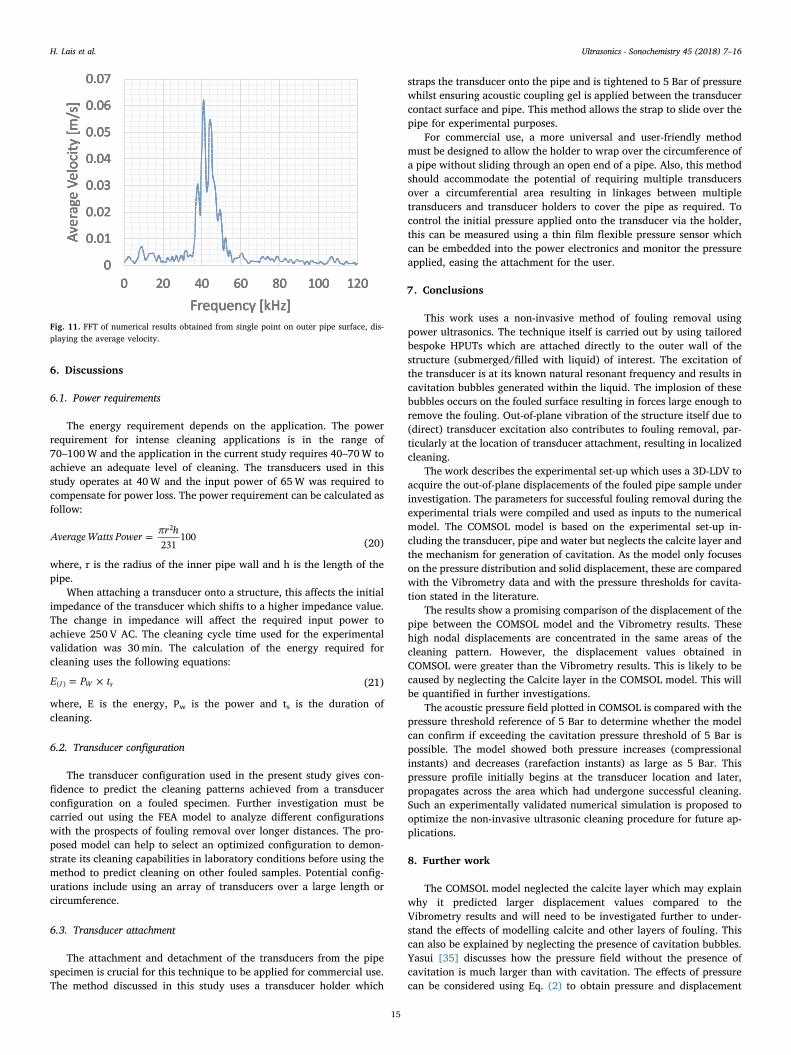
The COMSOL results were converted using FFT for ease of com-parison with the Vibrometry results. A single point is selected on thepipe surface to plot the out-of-plane displacement versus frequency.Fig. 11 shows a significant peak at 40 kHz, matching the vibrometryresults illustrated in Fig. 10. Overall there is a good agreement betweennumerical and experimental results of the consonant frequency for theinvestigated conditions.

Another clear comparison made from both Figs. 10 and 11 is be-tween the various peaks that follow the resonant harmonic in the Vi-brometry results that do not appear in the COMSOL model results. Thereason for this is that the Vibrometry analysis is obtaining data from aspecimen which is undergoing cavitation generation within the liquid.The cavitation bubbles emit shockwaves which resulted in the vibrationof the pipe wall at frequencies other than the operating frequency. TheCOMSOL model neglects the generation of cavitation bubbles whichmeans that there are no shockwaves being generated due to cavitationand result in frequency peaks other than at the resonance frequency.

Fig. 8. Comparison of results (a) experimentally obtained localized cleaning after one cycle of ultrasonic cleaning, (b) 3D displacement measured during ultrasonic cleaning using 3D-LDV, (c) numerical simulation results and (d) zoomed version of (c) displaying high displacement achieved at same location of cleaning and 3D-LDV results.

H. Lais et al. Ultrasonics - Sonochemistry 45 (2018) 7–16

13

Fig. 9. Numerical results displaying acoustic pressure of pipe filled with water at (a) 530ms and (b) 825ms and the isosurface plot of acoustic pressure at (c) 530ms and (d) 825ms.

Fig. 10. FFT of average velocity of scanned area using 3D-LDV measurements taken of 40 kHz HPUT attached to pipe geometry illustrated in Fig. 5.

H. Lais et al. Ultrasonics - Sonochemistry 45 (2018) 7–16

14

6. Discussions

6.1. Power requirements

The energy requirement depends on the application. The powerrequirement for intense cleaning applications is in the range of70–100W and the application in the current study requires 40–70W toachieve an adequate level of cleaning. The transducers used in thisstudy operates at 40W and the input power of 65W was required tocompensate for power loss. The power requirement can be calculated asfollow:

=Average Watts Power πr h231

1002

(20)

where, r is the radius of the inner pipe wall and h is the length of thepipe.

When attaching a transducer onto a structure, this affects the initialimpedance of the transducer which shifts to a higher impedance value.The change in impedance will affect the required input power toachieve 250 V AC. The cleaning cycle time used for the experimentalvalidation was 30min. The calculation of the energy required forcleaning uses the following equations:

= ×E P tJ W s( ) (21)

where, E is the energy, Pw is the power and ts is the duration ofcleaning.

6.2. Transducer configuration

The transducer configuration used in the present study gives con-fidence to predict the cleaning patterns achieved from a transducerconfiguration on a fouled specimen. Further investigation must becarried out using the FEA model to analyze different configurationswith the prospects of fouling removal over longer distances. The pro-posed model can help to select an optimized configuration to demon-strate its cleaning capabilities in laboratory conditions before using themethod to predict cleaning on other fouled samples. Potential config-urations include using an array of transducers over a large length orcircumference.

6.3. Transducer attachment

The attachment and detachment of the transducers from the pipespecimen is crucial for this technique to be applied for commercial use.The method discussed in this study uses a transducer holder which

straps the transducer onto the pipe and is tightened to 5 Bar of pressurewhilst ensuring acoustic coupling gel is applied between the transducercontact surface and pipe. This method allows the strap to slide over thepipe for experimental purposes.

For commercial use, a more universal and user-friendly methodmust be designed to allow the holder to wrap over the circumference ofa pipe without sliding through an open end of a pipe. Also, this methodshould accommodate the potential of requiring multiple transducersover a circumferential area resulting in linkages between multipletransducers and transducer holders to cover the pipe as required. Tocontrol the initial pressure applied onto the transducer via the holder,this can be measured using a thin film flexible pressure sensor whichcan be embedded into the power electronics and monitor the pressureapplied, easing the attachment for the user.

7. Conclusions

This work uses a non-invasive method of fouling removal usingpower ultrasonics. The technique itself is carried out by using tailoredbespoke HPUTs which are attached directly to the outer wall of thestructure (submerged/filled with liquid) of interest. The excitation ofthe transducer is at its known natural resonant frequency and results incavitation bubbles generated within the liquid. The implosion of thesebubbles occurs on the fouled surface resulting in forces large enough toremove the fouling. Out-of-plane vibration of the structure itself due to(direct) transducer excitation also contributes to fouling removal, par-ticularly at the location of transducer attachment, resulting in localizedcleaning.

The work describes the experimental set-up which uses a 3D-LDV toacquire the out-of-plane displacements of the fouled pipe sample underinvestigation. The parameters for successful fouling removal during theexperimental trials were compiled and used as inputs to the numericalmodel. The COMSOL model is based on the experimental set-up in-cluding the transducer, pipe and water but neglects the calcite layer andthe mechanism for generation of cavitation. As the model only focuseson the pressure distribution and solid displacement, these are comparedwith the Vibrometry data and with the pressure thresholds for cavita-tion stated in the literature.

The results show a promising comparison of the displacement of thepipe between the COMSOL model and the Vibrometry results. Thesehigh nodal displacements are concentrated in the same areas of thecleaning pattern. However, the displacement values obtained inCOMSOL were greater than the Vibrometry results. This is likely to becaused by neglecting the Calcite layer in the COMSOL model. This willbe quantified in further investigations.

The acoustic pressure field plotted in COMSOL is compared with thepressure threshold reference of 5 Bar to determine whether the modelcan confirm if exceeding the cavitation pressure threshold of 5 Bar ispossible. The model showed both pressure increases (compressionalinstants) and decreases (rarefaction instants) as large as 5 Bar. Thispressure profile initially begins at the transducer location and later,propagates across the area which had undergone successful cleaning.Such an experimentally validated numerical simulation is proposed tooptimize the non-invasive ultrasonic cleaning procedure for future ap-plications.

8. Further work

The COMSOL model neglected the calcite layer which may explainwhy it predicted larger displacement values compared to theVibrometry results and will need to be investigated further to under-stand the effects of modelling calcite and other layers of fouling. Thiscan also be explained by neglecting the presence of cavitation bubbles.Yasui [35] discusses how the pressure field without the presence ofcavitation is much larger than with cavitation. The effects of pressurecan be considered using Eq. (2) to obtain pressure and displacement

Fig. 11. FFT of numerical results obtained from single point on outer pipe surface, dis-playing the average velocity.

H. Lais et al. Ultrasonics - Sonochemistry 45 (2018) 7–16

15

values that match more similarly to the experimental results.In regards to the cleaning capabilities, there is potential for fouling

removal using the ultrasonic cleaning technique demonstrated by thelocalized cleaning results. However, optimization is the next step toimprove the coverage of cleaning which can be implemented using theproposed COMSOL model to determine the best array of transducers,frequency and other input parameters.

Further investigation on the technique itself are needed for im-proving its Technology Readiness Level (TRL). This includes in-vestigating the effects of coupling between the transducer contact sur-face and the fouled specimen to measure the change in cleaningcapabilities based on the use of acoustic coupling gel, dry contact andpermanently bonding the transducer onto the specimen.

By identifying the key factors in ensuring maximum cleaning, theprocedure for attaching/detaching transducers could be optimized forcleaning for commercial use and ease of use for the end user. Othersuggested factors include modification of the transducer contact sur-face, configuration of multiple transducers, cabling and power elec-tronics.

Acknowledgments

This investigation was conducted as part of Innovate UK projectsCleanMine and HiTClean, grant numbers 101333 and 102491, respec-tively. The authors express deep gratitude to Ignacio Garcia de Carellanand Makis Livadas of Brunel University London for all their efforts andcontributions to the projects and this work.

References

[1] A.S. Paipetis, T.E. Matikas, D.G. Aggelis, D. Van Hemelrijck, Emerging Technologiesin Non-Destructive Testing V, [Imprint] CRC Press, 2012.

[2] T. Yan, W.X. Yan, Fouling of offshore structures in China-a review, Biofouling 19(S1) (2003) 133–138.

[3] A.G. Pillai, A study on mitigating the effect of sulphates in lime stabilised Cochinmarine clays, PhD Thesis Cochin University of Science & Technology, India, 2014.

[4] M. Crabtree, D. Eslinger, P. Fletcher, M. Miller, A. Johnson, G. King, Fighting sca-le—removal and prevention, Oilfield Rev. 11 (3) (1999) 30–45.

[5] D. Yebra, S. Rasmussen, C. Weinell, L. Pedersen, Marine fouling and corrosionprotection for offshore ocean energy setups, 3rd Int Conf. Ocean Energy Bilbao,Spain, (2010).

[6] “Ocean Team Group as.” [Online]. Available: http://www.oceanteam.eu/.[Accessed: 14-Mar-2017]

[7] “Hilsonic.” [Online]. Available: http://www.hilsonic.co.uk/. [Accessed: 14-Aug-2017]

[8] “Ultrawave.” [Online]. Available: http://www.ultrawave.co.uk/. [Accessed: 14-Aug-2017]

[9] H. Maddah, A. Chogle, Biofouling in reverse osmosis: phenomena, monitoring,controlling and remediation, Appl. Water Sci. (2016) 1–15.

[10] M.O. Lamminen, Ultrasonic Cleaning of Latex Particle Fouled Membranes, PhDThesis Ohio State University, USA, 2004.

[11] H.-C. Flemming, Reverse osmosis membrane biofouling, Experim. Therm. Fluid Sci.14 (4) (1997) 382–391.

[12] C.E. Brennen, Cavitation and Bubble Dynamics, Cambridge University Press, 2013.[13] “Creation of stable and transient cavitation bubbles.” [Online]. Available: https://

www.hielscher.com/wp-content/uploads/stable-transient-cavitation-Santos-et-al.-2009-opt.png. [Accessed: 25-Jan-2018]

[14] K. Yasui, Acoustic Cavitation, Acoustic Cavitation and Bubble Dynamics, Springer,2018, pp. 1–35.

[15] M.P. Brenner, S. Hilgenfeldt, D. Lohse, Single-bubble sonoluminescence, Rev.Modern Phys. 74 (2) (2002) 425.

[16] R. Esche, Untersuchung der schwingungskavitation in flüssigkeiten, Acta Acusticaunited with Acustica 2 (6) (1952) 208–218.

[17] M.S. Plesset, A. Prosperetti, Bubble dynamics and cavitation, Ann. Rev. Fluid Mech.9 (1) (1977) 145–185.

[18] T. Mason, L. Paniwnyk, J. Lorimer, The uses of ultrasound in food technology,Ultrason. Sonochem. 3 (3) (1996) S253–S260.

[19] J.A. Gallego-Juarez, High-power ultrasonic processing: recent developments andprospective advances, Phys. Proc. 3 (1) (2010) 35–47.

[20] S. Lin, F. Zhang, Measurement of ultrasonic power and electro-acoustic efficiency ofhigh power transducers, Ultrasonics 37 (8) (2000) 549–554.

[21] S. Guo, B.C. Khoo, S.L.M. Teo, H.P. Lee, The effect of cavitation bubbles on theremoval of juvenile barnacles, Colloids Surf. B: Biointerfaces 109 (2013) 219–227.

[22] B. Lozowicka, M. Jankowska, I. Hrynko, P. Kaczynski, Removal of 16 pesticideresidues from strawberries by washing with tap and ozone water, ultrasoniccleaning and boiling, Environ. Monit. Assess. 188 (1) (2016) 1–19.

[23] B. Verhaagen, T. Zanderink, D.F. Rivas, Ultrasonic cleaning of 3D printed objectsand cleaning challenge devices, Appl. Acoustics 103 (2016) 172–181.

[24] L. Barnes, D. van der Meulen, B. Orchard, C. Gray, Novel use of an ultrasoniccleaning device for fish reproductive studies, J. Sea Res. 76 (2013) 222–226.

[25] D.D. Nguyen, H.H. Ngo, Y.S. Yoon, S.W. Chang, H.H. Bui, A new approach involvinga multi transducer ultrasonic system for cleaning turbine engines’ oil filters underpractical conditions, Ultrasonics 71 (2016) 256–263.

[26] V. Naddeo, L. Borea, V. Belgiorno, Sonochemical control of fouling formation inmembrane ultrafiltration of wastewater: effect of ultrasonic frequency, J. WaterProcess Eng. 8 (2015) e92–e97.

[27] M. Legay, Y. Allibert, N. Gondrexon, P. Boldo, S. Le Person, Experimental in-vestigations of fouling reduction in an ultrasonically-assisted heat exchanger,Experim. Therm. Fluid Sci. 46 (2013) 111–119.

[28] N.S.M. Yusof, B. Babgi, Y. Alghamdi, M. Aksu, J. Madhavan, M. Ashokkumar,Physical and chemical effects of acoustic cavitation in selected ultrasonic cleaningapplications, Ultrason. Sonochem. 29 (2016) 568–576.

[29] R. Jamshidi, Modeling and Numerical Investigation of Acoustic Cavitation withApplications in Sonochemistry, Papierflieger Verlag, 2014.

[30] G.L. Chahine, A. Kapahi, J.-K. Choi, C.-T. Hsiao, Modeling of surface cleaning bycavitation bubble dynamics and collapse, Ultrason. Sonochem. 29 (2016) 528–549.

[31] R. Mettin, P. Koch, W. Lauterborn, D. Krefting, Modeling acoustic cavitation withbubble redistribution, Sixth International Symposium on Cavitation, 2006, pp. 1–5.

[32] J. Lewis, S. Gardner, I. Corp, A 2D finite element analysis of an ultrasonic cleaningvessel: results and comparisons, Int. J. Model. Simul. 27 (2) (2007) 181–185.

[33] V.S. Moholkar, S.P. Sable, A.B. Pandit, Mapping the cavitation intensity in an ul-trasonic bath using the acoustic emission, AIChE J. 46 (4) (2000) 684–694.

[34] M. Hodnett, B. Zeqiri, N. Lee, P. Gélat, Report on the feasibility of establishing areference cavitating medium, NPL Report CMAM 58, National Physical Laboratory,Teddington UK, 2001.

[35] K. Yasui, Y. Iida, T. Tuziuti, T. Kozuka, A. Towata, Strongly interacting bubblesunder an ultrasonic horn, Phys. Rev. E 77 (1) (2008) 016609.

[36] M. Ashokkumar, Handbook of Ultrasonics and Sonochemistry, Springer, 2016.[37] K. Yasui, T. Kozuka, T. Tuziuti, A. Towata, Y. Iida, J. King, P. Macey, FEM calcu-

lation of an acoustic field in a sonochemical reactor, Ultrason. Sonochem. 14 (5)(2007) 605–614.

[38] Z. Wei, L.K. Weavers, Combining COMSOL modeling with acoustic pressure maps todesign sono-reactors, Ultrason. Sonochem. 31 (2016) 490–498.

[39] L. Zhong, COMSOL multiphysics simulation of ultrasonic energy in cleaning tanks,COMSOL Conference 2014 Boston, (2014).

[40] I. M. G. de C. Esteban-Infantes, Fundamentals of Pipeline Cleaning with AcousticCavitation, PhD Thesis, Brunel University London, UK, 2016.

[41] P. Lowe, R. Sanderson, N. Boulgouris, T. Gan, Hybrid active focusing with adaptivedispersion for higher defect sensitivity in guided wave inspection of cylindricalstructures, Nondestruct. Test. Eval. 31 (3) (2016) 219–234.

[42] P.S. Lowe, R.M. Sanderson, N.V. Boulgouris, A.G. Haig, W. Balachandran,Inspection of cylindrical structures using the first longitudinal guided wave mode inisolation for higher flaw sensitivity, IEEE Sens. J. 16 (3) (2016) 706–714.

[43] K. Yasui, T. Tuziuti, J. Lee, T. Kozuka, A. Towata, Y. Iida, Numerical simulations ofacoustic cavitation noise with the temporal fluctuation in the number of bubbles,Ultrason. Sonochem. 17 (2) (2010) 460–472.

H. Lais et al. Ultrasonics - Sonochemistry 45 (2018) 7–16

16