ultramicroscope ii – a user guide

UltraMicroscope II – A User Guide

Pablo Ariel, Ph.D. [email protected]

https://orcid.org/0000-0002-8494-0379

Assistant Professor Director of the Microscopy Services Laboratory

Department of Pathology and Laboratory Medicine University of North Carolina at Chapel Hill

September 2018, Chapel Hill, NC, USA.

mailto:[email protected]

https://orcid.org/0000-0002-8494-0379

Copyright notices

This work and associated files are licensed under the Creative Commons Attribution-NonCommercial 4.0 International License. To view a copy of this license, visit http://creativecommons.org/licenses/by-nc/4.0/ or send a letter to Creative Commons, PO Box 1866, Mountain View, CA 94042, USA.

Image in Figure 3.3 is reprinted from Cell, 159/4, Nicolas Renier, Zhuhao Wu, David J. Simon, Jing Yang, Pablo Ariel, Marc Tessier-Lavigne, iDISCO: A Simple, Rapid Method to Immunolabel Large Tissue Samples for Volume Imaging, Pages 896-910., Copyright 2014, with permission from Elsevier.

Top left image in Figure 5.1 reprinted by permission from Springer Nature: Nature, Structural and molecular interrogation of intact biological systems, Chung K, Wallace J, Kim SY, Kalyanasundaram S, Andalman AS, Davidson TJ, Mirzabekov JJ, Zalocusky KA, Mattis J, Denisin AK, Pak S, Bernstein H, Ramakrishnan C, Grosenick L, Gradinaru V, Deisseroth K, 2013.

Top right image in Figure 5.1 reprinted by permission from Springer Nature: Nature Protocols, Three-dimensional imaging of solvent-cleared organs using 3DISCO, Ertürk A, Becker K, Jährling N, Mauch CP, Hojer CD, Egen JG, Hellal F, Bradke F, Sheng M, Dodt HU., 2012.

Images in sample imaging and data visualization section of Figure 5.1 are reprinted from Neoplasia, 16/1, Michael Dobosz, Vasilis Ntziachristos, Werner Scheuer, Steffen Strobel, Pages 1-13, Copyright 2014, with permission from Elsevier.

Images in the data analysis section of Figure 5.1 is reprinted from Cell, 165/7, Nicolas Renier, Eliza L. Adams, Christoph Kirst, Zhuhao Wu, Ricardo Azevedo, Johannes Kohl, Anita E. Autry, Lolahon Kadiri, Kannan Umadevi Venkataraju, Yu Zhou, Victoria X. Wang, Cheuk Y. Tang, Olav Olsen, Catherine Dulac, Pavel Osten, Marc Tessier-Lavigne, Pages 1-14, Copyright 2016, with permission from Elsevier.

http://creativecommons.org/licenses/by-nc/4.0/

http://creativecommons.org/licenses/by-nc/4.0/

2 Contents

Contents 1 ADMINISTRIVIA ................................................................................................................................................... 4

1.1 WHO IS THIS FOR? .................................................................................................................................................... 4 1.2 WHY SHOULD YOU LISTEN TO ME? ............................................................................................................................... 4 1.3 WHY DID I WRITE THIS? ............................................................................................................................................. 4 1.4 WHAT THIS IS NOT .................................................................................................................................................... 4

2 SYSTEM BASICS ................................................................................................................................................... 5

2.1 BASIC PRINCIPLES OF SYSTEM OPERATION ...................................................................................................................... 5 2.2 WHAT IS THIS SYSTEM GOOD FOR? ............................................................................................................................... 5

3 SYSTEM CONFIGURATION ................................................................................................................................... 7

3.1 WHAT ARE THE MAIN CONFIGURATION OPTIONS? ........................................................................................................... 7 3.1.1 Zoom body vs infinity optics ......................................................................................................................... 7 3.1.2 White light laser vs individual laser lines ................................................................................................... 10

3.2 ACQUISITION COMPUTER SPECIFICATIONS .................................................................................................................... 11 3.3 WHAT ELSE WILL YOU NEED? .................................................................................................................................... 12

3.3.1 Air table ...................................................................................................................................................... 12 3.3.2 Fume hood ................................................................................................................................................. 12 3.3.3 Visualization/Analysis workstation ............................................................................................................ 12

4 RISKS ................................................................................................................................................................. 13

4.1 RISKS TO USERS ...................................................................................................................................................... 13 4.2 RISKS TO EQUIPMENT .............................................................................................................................................. 13

4.2.1 Crashing the objective into the sample ...................................................................................................... 13 4.2.2 A major spill of imaging solution out of the reservoir ................................................................................ 15 4.2.3 Dropping an objective or dipping cap ........................................................................................................ 15

5 WORKFLOW OVERVIEW .................................................................................................................................... 16

6 SAMPLE PREPARATION TIPS.............................................................................................................................. 17

6.1 TRIMMING TO THE BIOLOGICAL QUESTION ................................................................................................................... 17 6.2 CLEARING AND LABELING.......................................................................................................................................... 18

7 SAMPLE MOUNTING TIPS .................................................................................................................................. 19

8 OPTIMIZING IMAGING PARAMETERS ................................................................................................................ 22

8.1 INTRODUCTION ...................................................................................................................................................... 22 8.2 LIGHT SHEET PARAMETERS AND HOW TO ADJUST THEM OPTIMALLY ................................................................................... 23

8.2.1 Light sheet width ........................................................................................................................................ 23 8.2.2 Sheet NA and its effect on the shape of the light sheet in Z....................................................................... 25 8.2.3 Number of sheets: three vs. one ................................................................................................................ 27 8.2.4 Horizontal focus and sheetmotor calibration– positioning the sheet waist .............................................. 28 8.2.5 Laser power ................................................................................................................................................ 30

8.3 ADDITIONAL IMAGING CONSIDERATIONS ..................................................................................................................... 32 8.3.1 Imperfect light propagation through samples - imaging from both sides ................................................. 32 8.3.2 Radial aberrations in the optics ................................................................................................................. 34 8.3.3 Cropping ..................................................................................................................................................... 34

3 Contents

8.3.4 Tiling ........................................................................................................................................................... 35 8.3.5 Using the dynamic focus ............................................................................................................................ 36 8.3.6 Acquiring multi-channel images ................................................................................................................ 36

8.4 WORKFLOW SUMMARY AND EXAMPLES ...................................................................................................................... 38

9 ALIGNMENT TIPS ............................................................................................................................................... 42

10 DECONVOLUTION ........................................................................................................................................... 44

11 DATA TRANSFER.............................................................................................................................................. 45

11.1 DEFINING THE PROBLEM ........................................................................................................................................ 45 11.2 DEFINING OTHER PROBLEMS THAT THE UNC CORE CANNOT SOLVE QUICKLY, CHEAPLY OR AT ALL ......................................... 45 11.3 CONSTRAINTS ...................................................................................................................................................... 45 11.4 NARROWING THE PROBLEM .................................................................................................................................... 46 11.5 CURRENT CONFIGURATION IN THE UNC CORE ............................................................................................................ 46 11.6 THOUGHTS ABOUT EVEN BIGGER DATASETS ................................................................................................................ 47

12 VISUALIZATION/ANALYSIS WORKSTATION ..................................................................................................... 48

13 ACKNOWLEDGEMENTS ................................................................................................................................... 51

14 REFERENCES .................................................................................................................................................... 52

ANNEX - STANDARD OPERATING PROCEDURES UNC ........................................................................................... 53

START UP .................................................................................................................................................................... 53 MOUNTING THE SAMPLE................................................................................................................................................ 53 FINDING THE SAMPLE .................................................................................................................................................... 54 IMAGING SETUP – THE BASICS ......................................................................................................................................... 55

Focusing evenly across the X dimension ............................................................................................................. 55 Exposure and laser power ................................................................................................................................... 55 Imaging with both light sheets (OPTIONAL): ...................................................................................................... 55 Imaging with multiple horizontal X sheet foci (OPTIONAL): ............................................................................... 56 Cropping .............................................................................................................................................................. 56 Autosave settings ................................................................................................................................................ 56

EXPERIMENT DESIGNS ................................................................................................................................................... 57 Acquiring Z stack – 1 channel: ............................................................................................................................. 57 Acquiring Z stack – more than 1 channel: ........................................................................................................... 58 Generating a Mosaic Image: ............................................................................................................................... 59

VIEWING DATA IN IMSPECTOR ........................................................................................................................................ 60 CHANGING SAMPLES ..................................................................................................................................................... 61 SHUT DOWN................................................................................................................................................................ 62

4 1 Administrivia

1 Administrivia

1.1 Who is this for? Members of labs or core facilities who already have, or want to install, a LaVision BioTec UltraMicroscope II light sheet system (Fig. 1.1).

1.2 Why should you listen to me? I’ve worked in two cores (at Rockefeller University and the University of North Carolina at Chapel Hill) where this microscope was implemented. Over the past four years I’ve gained hundreds of hours of experience with the system using samples from more than 40 labs from a dozen institutions. Along the way, I’ve made a lot of mistakes, learned from them, and improved our procedures. I’ve also benefitted enormously from many discussions with colleagues facing the same challenges. Finally, I don’t work for LaVision BioTec and am not interested in selling you a microscope; I’m trying to present an honest assessment of the benefits and pitfalls of this instrument, and some best practices, based on my experience as a user.

1.3 Why did I write this? To help other users avoid reinventing the wheel. I believe this technology is mature enough that we should all share a baseline of best practices that is easily accessible to anyone with this microscope. We can (and should!) continue to improve our procedures, as well as quibble about many details, but I strongly believe all users should have a foundation of knowledge on which to build their own implementation of the system.

1.4 What this is not A guide for tissue clearing and labeling, a detailed manual for using the software, a recipe for the single best way to image samples with this microscope, or a guide to image analysis. For clearing and labeling, there is prolific literature to consult. For the ImSpector Pro software, LaVision BioTec provides a manual, as well as training during installation. For the imaging, there is no “best” way, only a multitude of options with different tradeoffs, which I will discuss at length. How to analyze images is a vast topic in which my expertise barely scratches the surface.

Figure 1.1. LaVision BioTec UltraMicroscope II, zoom optics version.

5 2 System basics

2 System basics

2.1 Basic principles of system operation The system uses cylindrical lenses to generate three sheets of laser light that can illuminate a cleared sample from the side. Excitable fluorophores in the illuminated plane emit red-shifted photons, which are collected by an objective orthogonal to the sheet. These photons then go through additional magnification optics, emission filters, and a chromatic correction module and are imaged on a sCMOS camera. The system can illuminate samples from the right or left side and merge the views. The three sheets illuminating the sample are slightly tilted (in the XY plane) to allow visualization behind opaque portions of the sample. Each sheet has a narrow waist, where thickness in Z is minimal (it can be as thin as 5 µm), and then flare out as the distance from that waist position in the X dimension increases. Both the position of the waist and the exact shape and thickness of the sheets can be controlled in the software. By lowering the sheet numerical aperture (NA), the system can create sheets that are thicker in Z, but more even as they propagate along the X dimension. Views from multiple sheets focused at different X positions can be merged in the software, to have a more even Z resolution. The system has a motorized stage and supports tiling for large samples.

The sample is held by a custom holder immersed in a reservoir with a fluid of choice that can be almost any of the liquids used in the final clearing step of many protocols, including those that use organic solvents (Fig. 2.1). Due to toxicity and corrosion considerations, use of Benzyl Alcohol/ Benzyl Benzoate (BABB) in the imaging chamber—while possible—is not recommended. On the other hand, use of dibenzyl ether is routine. The sample holder does not support sample rotation, and the imaging chamber does not have climate control (a separate module for this application can be purchased).

2.2 What is this system good for? In short, cellular questions in large (several millimeters in diameter), cleared, fixed samples.

The main advantages of the system are:

1. High speed in acquiring very large volumes of data (in XYZ), compared to a laser scanning confocal. The imaging speed depends on the exact details of the acquisition, but half an adult mouse brain at around 5 µm resolution in approximately 1.5 hours per channel is a good benchmark.

2. Decreased photobleaching, compared to confocal.

Figure 2.1. Diagram of sample in holder inside reservoir with clearing solution. Source: LaVision BioTec promotional materials

6 2 System basics

3. Compatibility with organic solvents used in many effective clearing methods (such as dibenzyl ether used in 3DISCO and iDISCO+).

4. Ability to accommodate very large samples. In Z, the limiting factor is the working distance, which can be up to 5-10 mm, depending on the objective. In XY, dimensions can be up to 50 mm, though this is not practical in the direction over which the light sheet propagates; no matter how cleared a sample is, there will still be significant distortions in light propagation over very long distances. Less than 10 mm in the X dimension is probably a more realistic upper bound, while the Y dimension can be up to 50 mm (though this requires tiling).

The main disadvantages of the system are reduced resolution in XY, and even more reduced in the Z dimension, compared to a laser scanning confocal.

The resolution in XY depends on the exact objective or zoom factor but ranges between 1-10 µm. Resolution in Z depends on the sheet width and where in the field of view the structure of interest is. It can vary between 5 µm at the smallest to many tens of microns, or worse. I go into considerably more detail on this point in the optimizing imaging parameters section (8).

Even though the resolution of the system is several microns or worse, objects smaller than that (for example, 0.2 µm diameter axons) can be visualized, as long as they are fluorescently labeled. They will appear larger than their actual dimensions, but they will be visible. The key is whether the objects of interest are spaced far enough apart from each other to be identified as separate objects, not how big they are. This is a general point about resolution independent of the details of this light sheet microscope, but it is particularly salient here, given the substantially worse resolution than a typical confocal, especially in Z.

Examples of good research questions for this system:

• Studies of vasculature, lymphatic vessels, and airways in the lung. The size and spacing of these objects is ideal for the resolution of the system.

• Attempts to find a sparse subset of labeled cells in a large sample (be it an entire rodent organ, a rodent tumor, a mouse embryo or a biopsy from a larger animal). There are many biological questions of this general kind: activated neurons in the brain, metastatic cells in an organ, etc.

• Tracing all targets of neurons that send projections out from a particular brain region.

Examples of bad research questions for this system:

• Anything subcellular (example: counting spines in neurons). • Counting the number of cells in very densely labeled tissue. • Tracing individual axons in densely labeled tissue. • Anything that requires live imaging over prolonged periods of time. While LaVision BioTec sells a

live cell module made by Okolab, the basic constraint is that the chamber is open. Therefore, any gas control will be limited, and the open bath can run into contamination and evaporation issues over long periods of time.

7 3 System configuration

3 System configuration

3.1 What are the main configuration options? 3.1.1 Zoom body vs infinity optics The former uses a single Olympus MVPLAPO 2X/0.5 objective with a custom LaVision BioTec dipping cap, coupled to a zoom body with total magnifications that can range from 1.26X to 12.6X by turning a zoom knob. The latter involves individual objectives manufactured by LaVision BioTec (there are three main ones that I know of: a 1.3X/0.1, a 4X/0.28, and a 12.6X/0.53), as well as additional magnification lenses (1, 2 and 4X in sliders or turrets are available).

The main advantage of the zoom body is its simplicity: a change in magnification only requires a change in a knob position. The disadvantage is that the quality is lower than the infinity optics configuration. How much lower is unclear, as LaVision BioTec has not published any detailed comparisons with standard samples. This is problematic, as doing these detailed comparisons is very difficult for a prospective user who does not have access to both systems. In addition, these comparisons take a considerable amount of time and require a large, high-quality sample with evenly distributed staining in structures of varying sizes. Anecdotally, in head-to-head testing on a brain with labeled vasculature (using the sample shown in Figs. 8.11 and 8.12), I saw slightly better performance of the 4X/0.28 infinity objective compared to the 4X magnification setting of the zoom optics, using a corrected dipping cap. Also anecdotally, I have seen examples of data (at the 2018 LaVision BioTec meeting) taken with the 12.6X/0.53 objective compared to data taken with the equivalent magnification on the zoom optics; the former was significantly better. Unfortunately, without more extensive and published comparisons, it is impossible to rigorously compare the optical quality of the zoom body and infinity optics.

Another difference between the zoom body and infinity optics are the working distances of the objectives, which are generally larger in the latter configuration. The zoom optics objective must be used with custom dipping caps manufactured by LaVision BioTec, of which there are various models. Three old models of dipping caps came in 4, 6 and 10 mm working distances, with progressively lower quality for the longer distances, which showed very noticeable distortions in the image around the edges of the field of view. There is also a more recent “corrected” dipping cap with a 5.7 mm working distance, which has a lens inside that corrects for some of the aforementioned distortions. While 5.7 mm is the working distance of the 4X/0.28 objective, the 1.3X/0.1 objective (which does not dip into the reservoir with clearing solution) for practical purposes has an unlimited working distance and the new 12X/0.53 objective has a 10 mm working distance. In summary, the zoom body either has a shorter working distance at many magnifications (using the corrected dipping cap) or a similar working distance with significantly poorer quality (10 mm working distance dipping cap).

A final disadvantage of the zoom optics is that the objective has a larger diameter than the infinity optics objectives. Because of the limited clearance between the sample chamber and the objective, this makes it harder to do high resolution tiling on the edges of large samples (the objective can bump into the edges of the chamber under those conditions; see Fig. 3.1).


As far as the infinity optics go, while their quality is better (though by how much is unclear), they are more expensive and have some usability problems.

The configuration of the system is such that when a sample needs to be changed, the 4X lens needs to be removed from the system before removing the sample (this is probably also true of the 12.6X—given its size—though I have not tested that personally; the 1.3X/0.1 does not need to be removed). The problem is that the lens cannot be racked up far enough to allow the sample holder to be comfortably removed with the objective still on the system; there is simply not enough clearance. In contrast, on the zoom body configuration, the 2X objective sits on a revolver that can easily be swung out of the way (Fig. 3.2). This means that each time a sample is changed, the objective has to be cleaned (if not, potentially toxic and corrosive solvents can drip all over the system and possibly get inside the objective optics), removed from the system, and placed into some sort of holder, all of which makes the workflow quite annoying for a user. To avoid contamination during these steps, a user will need to put on gloves to clean the solvents off the objective, remove gloves to handle the objective without contaminating it, put the objective aside in a padded box or appropriate holder, put gloves back on, change the sample, remove gloves and put the objective back on the system. All of these steps add time and a number of annoying glove changes to the workflow. They also increase the likelihood of mistakes. The objectives are expensive and heavy, and the need to remove and put them back every time a sample is changed can be very dangerous in a multi-user facility with high usage; dropping an objective can have catastrophic consequences.

Figure 3.1. View from the top of the sample chamber, illustrating the problems with imaging edges of long (in the Y dimension) samples at high magnification, with the zoom body 2X objective. Centering the sample (as shown here; also see Fig. 7.1) can ameliorate but not eliminate this problem. This is less of an issue with the 4X infinity corrected lens, which has a smaller diameter.


In my opinion, the zoom body is generally the better configuration for a multi-user core facility, while the infinity optics are probably best in an individual lab or in a core where the staff does the imaging for the users. If a lot of researchers need the instrument for higher resolution applications combined with tiling, this can tilt the scales toward the infinity optics, even if the instrument will be in a core. In the core at the University of North Carolina at Chapel Hill, I opted to purchase the zoom body model. If a lab decides to buy both configurations, this will result in a considerably larger upfront expense, and there is the added issue that swapping between configurations is an operation that takes a trained person at least 30 to 40 minutes. Thus, it is not practical to swap back and forth multiple times a day, and the swapping adds major inefficiencies to the operation of the system (the need for infinity days and zoom body days, staff or lab member time budgeted for swapping, etc.).

Figure 3.2. The difficulty in removing the sample when using the 4X objective in the infinity optics configuration, compared to the 2X objective in the zoom body configuration.

Infinity optics – 4X objectiveNot enough clearance to exchange sample without removing objective.

X4X

4X

2X

2X

Zoom optics – 2X objectiveSufficient clearance to exchange sample without removing objective.


3.1.2 White light laser vs individual laser lines The white light laser covers the visible-IR region of the spectrum (but not the UV, which fortunately is not very limiting, see below). For individual laser lines, pretty much anything can be selected, and up to five lines can be combined.

The advantage of the white light laser is that it is cheaper and more flexible: different filter sets allow different excitation options, and this can be changed easily and cheaply after purchase. The disadvantages of the white light laser are the lower power density at any particular wavelength (which may require longer exposures, and therefore longer acquisition times), and the fact that if the laser fails it will take down the whole system and the repairs can take many weeks (because these lasers are rarer and LaVision BioTec coordinates repairs with NKT photonics, the original manufacturer).

For individual laser lines, the main advantage is higher power at a given wavelength, which allows shorter exposures and faster acquisition. With multiple channel acquisitions the speed advantage gets diluted because of the need to switch the emission filter (which is on a mechanical wheel) and move the chromatic correction lens in the system. While a dual emission filter could circumvent the former issue (at the cost of potential crosstalk), the chromatic correction is unavoidable, particularly so at high magnifications where the need for this correction is more acute (see the multi-channel imaging section (8.3.6)). Another advantage of using individual laser lines is that if one of them fails, this will not take down the entire system, and repairs can be (in theory) faster and cheaper. The main disadvantages of individual lasers are potentially higher upfront costs (depending on the number and specific lines selected), and the higher cost to change things later (as a new laser is needed, not just a new filter).

If the decision is made to purchase individual laser lines, the next question is which ones to buy (for the white light laser option the analogous—cheaper—decision is which excitation filters to buy). Because of increased scattering, autofluorescence and absorption, anything below 488 nm (for example 445 nm, 405 nm) is likely to be a bad investment; it is very hard to pick up good CFP or UV dye signals in that region of the spectrum in large cleared samples. A typical laser combination is 488 nm, 561 nm and 647 nm. The 488 nm can be used to image very brightly expressed GFP, bright staining or autofluorescence (in rodent brain samples, this can be used for automatic registration and segmentation), while the 561 nm can be used for RFP and staining and the 647 nm for staining. The improvement in signal-to-noise due to reduced autofluorescence, scattering and absorption can be substantial at longer wavelengths (Fig. 3.3), so if there is room in the budget for additional far(ther) red lasers these can be a good investment. In the UNC Core, we have a 785 nm, which we have used successfully with Alexa 790 (while the camera QE is lower in the part of the spectrum, scattering, autofluorescence and absorption are dramatically reduced). Other potential lasers to consider are 685 nm (for reasons similar to the 785 nm) and 514 nm. The 514 nm can help disentangle the various fluorophores if a CFP+GFP+YFP+RFP (“confetti”) mouse model is used. It is unlikely that direct visualization of CFP would be effective in a large cleared sample (I have not seen any good examples of this), but staining for the jellyfish-derived proteins (CFP, GFP, YFP) in the far red, imaging GFP (with the 488 nm laser), YFP (with the 514 nm laser), RFP (with the 561 nm laser) and CFP+GFP+YFP (with the far red laser) could separate them with some basic subtraction. I have not had the opportunity to try this scheme out on the UltraMicroscope II, but I have seen it work on a confocal, so in principle it should be doable. In the UNC Core, we have 488 nm, 514 nm, 561 nm, 647 nm, and 785 nm because some local researchers were interested in confetti mice. If not for that, we would have likely tried to purchase a 685 nm laser to have one more nicely spaced


line close to an Alexa dye (Alexa Fluor 680 or 700) in the infrared, low autofluorescence region of the spectrum.

3.2 Acquisition computer specifications With the UltraMicroscope II light sheet will come the challenge of big datasets, which users will want to visualize, analyze, transfer and store. Which of those functions will be your lab or core’s responsibility will influence what investments you make in the acquisition computer, the analysis workstation (that you will need to buy separately, see the visualization/analysis workstation section (12)), the cables and network switches in your physical space, and any data storage solutions. If you don’t have some sort of plan for everything that comes after data acquisition, the light sheet by itself will not live up to its full potential.

The approach we have taken in the UNC Core facility is to set up a separate workstation for visualization and—basic—analysis, and to maximize transfer speeds from the acquisition computer to that workstation. I provide strong support for visualizing data, less (or no) support for more complicated analysis, and no support at all for long-term data storage, offloading that responsibility onto my users.

With all of this in mind, I will discuss the non-standard items I’ve added to the acquisition computer. The UNC Core is only wired with 1 Gb Ethernet, so we’ve implemented two things to speed up data transfers to the analysis workstation:

Figure 3.3. Using fluorophores with longer wavelengths results in higher quality images due to reductions in autofluorescence, scattering and absorption at those higher wavelengths. TrkA staining in E14.5 embryos. Note the significantly reduced autofluorescence in the liver (see arrow). Modified from Renier et al, 2014, Fig S1.


• Second Ethernet card on the acquisition computer that supports 10 Gb. I also have a 10 Gb card on the analysis workstation, and the acquisition computer is connected directly to it. Note that the cable connecting these is a Cat 5e Ethernet cable that can only be up to around 100 meters long. This helps keep transfer times for datasets smaller than 100 Gb manageable, but is not sufficient for comfortable transfers of TB-sized datasets (which are not typical, but can arise from high resolution tiling). We don’t always reach peak expected speeds (for reasons that are not clear, given that it is a direct connection) and setting this up required some support from our IT department to get the two computers talking to each other over the direct connection. In my opinion, the increase in transfer speed was worth the investment of time and money.

• Hot swap bay with a 2 TB+ SSDs. This maximizes transfer speeds to sneakernet1 values, and is by far the fastest and cheapest way of doing things. In addition, people can use their own hard drives, and speed up data movement between the acquisition computer, our analysis workstation, and their own computers in their labs.

The issue of data transfer is addressed at more length in its own section (11).

3.3 What else will you need? 3.3.1 Air table LaVision BioTec can provide detailed requirements, which are fairly standard. At UNC, we have a 900x1200 mm smooth top table from TMC (item #s: 63-9012S, 81-301-12, 83-014-01).

3.3.2 Fume hood It is essential that a fume hood be as close to the microscope as possible as it will be used to mount samples prepared with organic solvents, and to periodically change the solution in the microscope’s reservoir. Less distance to the microscope means lower chances of spills en route to the system. Any fume hood is probably fine; at UNC, we have a small benchtop model from Labconco (Protector XVS, item # 4862010), as well as a chemically resistant tray from Fisher that we place inside to contain any potential spills (item # 3054031537; originally suggested by Kaye Thomas, in the Rockefeller University imaging core).

Some labs enclose the entire microscope in a custom fume hood or place an exhaust system close to the microscope to further minimize accumulation of any fumes from organic solvents in the microscope’s reservoir.

3.3.3 Visualization/Analysis workstation This is an important and complicated topic, so I have devoted a separate section to it (12).

1 https://en.wikipedia.org/wiki/Sneakernet

13 4 Risks

4 Risks There are two categories of risk when using this microscope: to the users, and to the equipment.

4.1 Risks to users The main risk for users is exposure to toxic chemicals used for certain clearing techniques that can be present inside the imaging reservoir. The way we mitigate these risks at UNC is to:

1. Place very clear signage indicating which components should only be touched with gloves (marked with red tape) and which should never be touched with gloves (marked with green tape).

2. Design procedures for mounting samples that minimize the number of times people need to put on and remove their gloves (see the Standard Operating Procedures in the ANNEX (SOPs)).

3. Strongly emphasize safe handling procedures during training and subsequent interactions with users.

4.2 Risks to equipment The main risks for the equipment are crashing an objective into a sample, a chemical spill or dropping an objective or dipping cap.

4.2.1 Crashing the objective into the sample

For the infinity optics, this can cause thousands of dollars of damage to an objective. For the zoom optics, this can destroy a corrected dipping cap costing hundreds of dollars. To reduce this risk, at UNC we do the following:

1. Have multiple signs indicating how movement of various knobs affects the distance between objective and sample (Fig. 4.1).

2. Have red “risk markers” indicating caution for the two operations that can bring sample and objective together: lowering the objective, raising the sample (Fig. 4.1).

Figure 4.1. Signage indicating how various knobs move the sample and objective, with clear caution warnings for certain risky operations.

14 4 Risks

3. As part of our sample-finding procedures (see SOPs): a. Confirm by eye that a clearly visible light sheet (we recommend 561 nm) is physically

going into the sample. Trying to lower the objective without confirming the light sheet is hitting the sample is a recipe for disaster (as the user will never see the sample appear on the screen), so it is critical to emphasize this step during training.

b. Move the sample such that the light sheet intersects it near the top (in Z). This corresponds to a sample that is farther from the objective and increases the safety margin when moving the objective to find the sample (as shown in the situation on the left of the large sign in Fig. 4.1, right).

c. Start focusing the sample on the camera at the lowest magnification, which makes it less likely that the illuminated portion of the sample will be outside the field of view and therefore not visible as the objective moves down towards it.

d. Once the illuminated portion of the sample is in focus on the camera at low mag, move the sample down until the light sheet is out of the sample and mark that as the 0 position. From then on, keep track of the position and ensure the stage position does not exceed 5200 µm below the surface of the sample marked as 0 (which is the 5.7 mm rated working distance of the corrected dipping cap minus a 0.5 mm safety margin).

e. Never mount samples noticeably protruding beyond the standard 5 mm high posts in the LaVision BioTec sample holders. If they do, that means there will likely be sample space beyond the working distance. Thus, if a user does not keep close track of their Z position relative to the top of the sample, they might not realize it if they go too deep into it, raising the sample towards the objective, and crashing (Fig. 7.1, bottom).

f. Always set up Z stacks so that they start with the light sheet deep in the sample (in Z), and end with the light sheet intersecting the top of the sample (Fig. 4.2). With this configuration, at the end of the Z-stack the sample will be far from the objective, so any mistakes moving the objective or sample too forcefully in the “wrong” direction (towards each other) after taking the Z stack will have a large safety margin.

Figure 4.2. Recommended setup for Z stacks, to minimize chance of objective crashing into sample.

x

z

Start Z stack at bottom of sample

End Z stack at top of sample

Objective ObjectiveDuring Z stack sample will move away from objective.

After Z stack sample will be far from objective

…

15 4 Risks

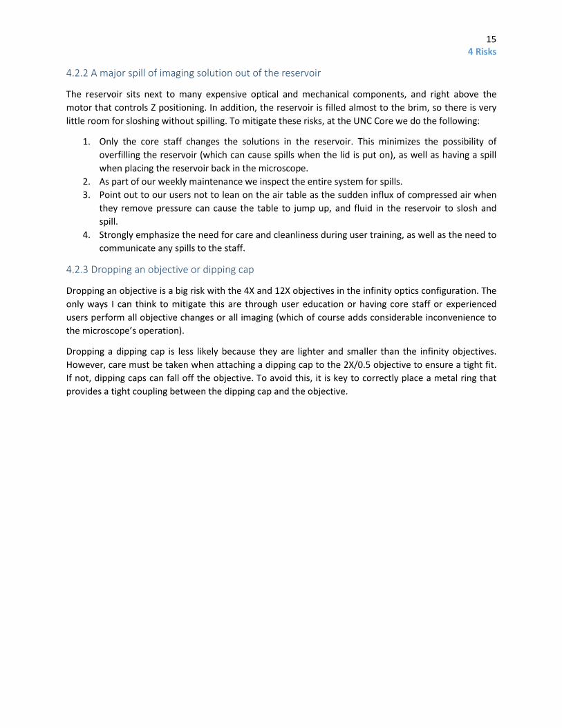
4.2.2 A major spill of imaging solution out of the reservoir

The reservoir sits next to many expensive optical and mechanical components, and right above the motor that controls Z positioning. In addition, the reservoir is filled almost to the brim, so there is very little room for sloshing without spilling. To mitigate these risks, at the UNC Core we do the following:

1. Only the core staff changes the solutions in the reservoir. This minimizes the possibility of overfilling the reservoir (which can cause spills when the lid is put on), as well as having a spill when placing the reservoir back in the microscope.

2. As part of our weekly maintenance we inspect the entire system for spills. 3. Point out to our users not to lean on the air table as the sudden influx of compressed air when

they remove pressure can cause the table to jump up, and fluid in the reservoir to slosh and spill.

4. Strongly emphasize the need for care and cleanliness during user training, as well as the need to communicate any spills to the staff.

4.2.3 Dropping an objective or dipping cap

Dropping an objective is a big risk with the 4X and 12X objectives in the infinity optics configuration. The only ways I can think to mitigate this are through user education or having core staff or experienced users perform all objective changes or all imaging (which of course adds considerable inconvenience to the microscope’s operation).

Dropping a dipping cap is less likely because they are lighter and smaller than the infinity objectives. However, care must be taken when attaching a dipping cap to the 2X/0.5 objective to ensure a tight fit. If not, dipping caps can fall off the objective. To avoid this, it is key to correctly place a metal ring that provides a tight coupling between the dipping cap and the objective.

16 5 Workflow Overview

5 Workflow Overview

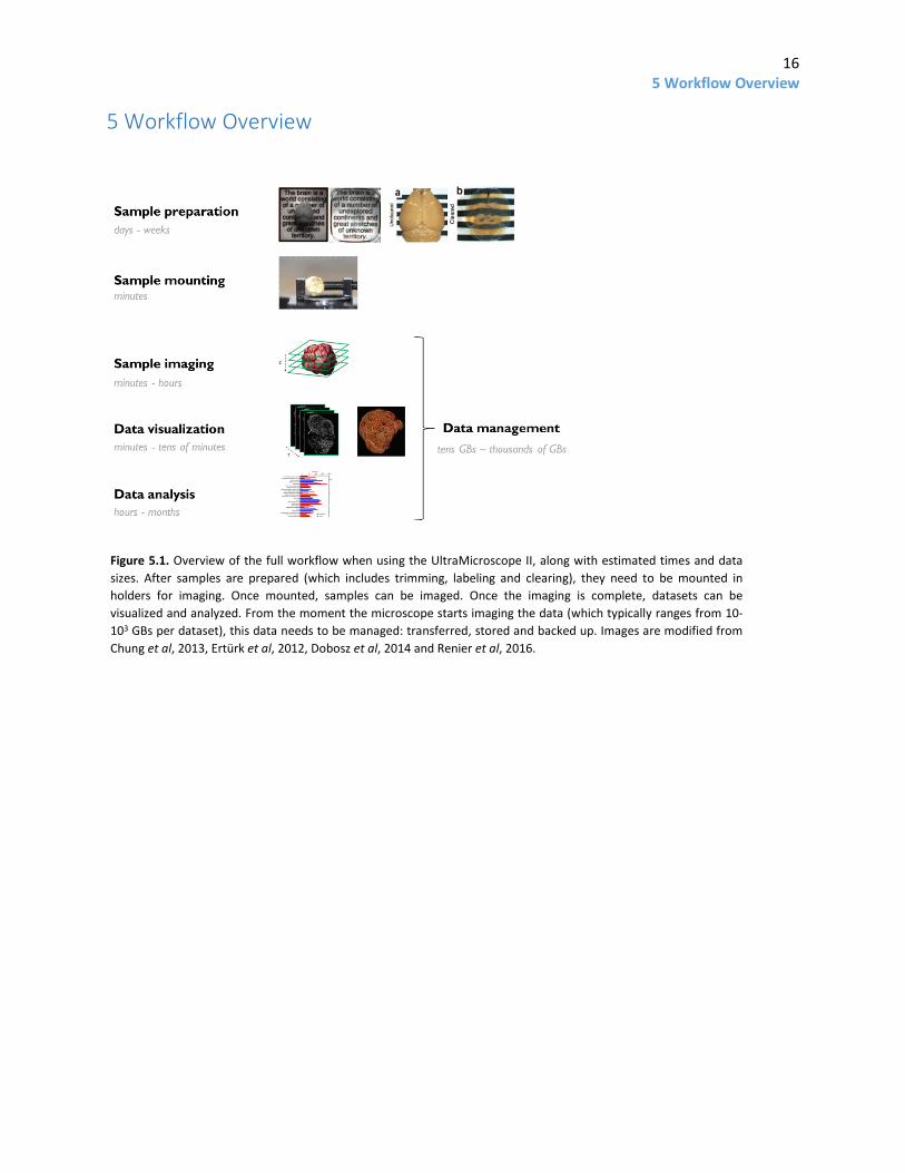
Figure 5.1. Overview of the full workflow when using the UltraMicroscope II, along with estimated times and data sizes. After samples are prepared (which includes trimming, labeling and clearing), they need to be mounted in holders for imaging. Once mounted, samples can be imaged. Once the imaging is complete, datasets can be visualized and analyzed. From the moment the microscope starts imaging the data (which typically ranges from 10-103 GBs per dataset), this data needs to be managed: transferred, stored and backed up. Images are modified from Chung et al, 2013, Ertürk et al, 2012, Dobosz et al, 2014 and Renier et al, 2016.

17 6 Sample preparation tips

6 Sample preparation tips Sample preparation includes trimming, labeling with fluorophores (if the tissue does not express them endogenously) and tissue clearing.

6.1 Trimming to the biological question Sample trimming is an often ignored step during sample preparation. We recommend users trim their sample to their biological question (Fig. 6.1). While there is often a temptation to image bigger samples (such as whole brains), this is often unnecessary (for example, if labeled neurons are restricted to a small part of the brain) and can add significant costs. Smaller samples clear faster, can be immunostained more quickly and with less antibody, are easier to image (no matter how transparent samples look, there will always be distortions when light propagates through them) and can be imaged more quickly. In addition, trimming can make samples with unconventional shapes easier to mount in the microscope by turning them into a block. In short, trimming a sample is a simple way for users to save time and money. Note that if a sample is trimmed down to be very small (on the order of 1-2 mm in diameter), this can make it challenging to mount in a sample holder. I address this challenge in the sample mounting tips section (7).

Figure 6.1. Examples of trimming samples to match the expected distribution of neurons under study. Note that all relevant regions are included, but samples are scaled properly to those regions of interest. This saves time and reagents for clearing and labeling (if needed), and makes the sample easier and faster to image due to its smaller size.

Original samples

Trimmed

18 6 Sample preparation tips

6.2 Clearing and labeling There are many effective labeling and clearing methods in the literature, as well as several good reviews that summarize them (see Ariel 2017 for references to the methods I have found most useful). One of the main advantages of the LaVision BioTec UltraMicroscope II is its compatibility with organic solvents, which allows users access to some of the fastest and most effective clearing techniques. In the UNC Core, we have had great success with iDISCO+ (full disclosure: I am an author on the paper describing the first iteration of iDISCO), and BABB-based methods (which we image in DBE). I have also seen acceptable results with uDISCO (if the endogenous fluorophores are not RFPs and are expressed at a very high level), CUBIC (in the superficial 2-3 millimeters of cleared samples) and PACT (though the samples are very soft and harder to mount). These observations should not be taken as rigorous comparisons between any of the methods, and it is important to note that the success of any clearing method is highly sample dependent. When I consult with people on which clearing/labeling method to use, I advise them to copy one that has already worked for a similar sample type and biological question, that has not only been used by the lab that created it, that requires minimal equipment and has a low implementation cost. In the UNC Core, that frequently means iDISCO+. However, in your own lab or core, you may find other techniques more suitable for your own research. Several clearing and labeling methods (particularly in the CLARITY family) require specialized equipment but this may not be a limiting factor if there is a sample clearing/labeling service at your institution (that is not the case at UNC).

With respect to labeling samples, using fluorophores with longer wavelengths is a big advantage, as there is less autofluorescence, scattering and absorption at longer wavelengths (Fig. 3.3). In fact, the combination of these factors can make it very difficult to image successfully in the green, cyan or blue channels, unless the fluorophore concentration is very high. Thus, even if fluorescent proteins are in the sample, it can be advantageous to immunolabel them to amplify signals (the typical multiplicative effect of primary and secondary staining) and spectrally shift them to longer wavelengths. In our core, users have had particular success combining AlexaFluor dyes 568, 647 and 790 with the iDISCO+ technique. While longer wavelengths lead to lower resolution, the effect is negligible on this microscope, given that its maximal resolution is not high enough for this wavelength dependence to make an appreciable impact on image quality.

19 7 Sample mounting tips

7 Sample mounting tips How the sample is placed in the holder for imaging is very important for successful imaging (Fig. 7.1).

Mounting the sample such that it is narrower in the X dimension is advantageous, because it minimizes light propagation through the sample. The excitation light is more likely to suffer distortions the further it propagates through a sample, no matter how clear a sample is, so minimizing the travel distance is a good way to reduce potential problems. Relatedly, if the structures of interest tend to be on one side of the sample (for example, the spinal cord of an embryo), it can be convenient to place those structures on the side and illuminate with a light sheet from the same side to minimize the distance the light has to travel into the sample to reach them.

Placing the regions of interest near the top of the sample is convenient for similar reasons. The deeper one looks into the sample, the farther the emitted photons need to travel through that sample to reach the objective. Thus, if samples are not perfectly clear, structures farther from the objective can be harder to visualize.

For samples that have standard orientation planes in histological atlases devised from sections (like brains, with sagittal and coronal sections), it can be convenient to place the sample such that one of those planes aligns with the XY imaging plane. This can simplify visualization and exploration of the resulting datasets.

It is a good idea to center samples in the holder in the X and Y axis as much as possible (for example, by using LaVision BioTec holders with thicker posts in the case of small samples, as shown in Fig. 7.1, third row left). If high resolution tiling is needed, portions of the sample that are near the edges of the mount can be impossible to reach with the objective due to the limited clearance between the objective and the reservoir opening. This is a particular concern with the zoom optics, in which the objective is very large compared to the reservoir opening (Fig. 3.1); it is less of a concern with the infinity optics, in which the objectives either don’t dip into the reservoir (1.3X/0.1) or do, but have a smaller diameter (for the 4X/0.28).

Figure 7.1. Recommendations for optimal sample mounting.


As mentioned in the risks to equipment section (4.2), to avoid expensive damage, it is a good idea to not exceed the working distance of the objective when mounting samples in the Z dimension.

Unfortunately, it is often impossible to satisfy all these criteria at once. In those cases, it is best to try a few orientations, image Z stacks in each one and from the resulting data decide which one works best. We strongly recommend this to our users, as sample orientation can have a dramatic effect on image quality and is very easy to test and optimize.

LaVision BioTec provides a number of default sample holders or mounts, most of which are quite convenient. We have expanded the functionality of these in two ways. First, we have designed pedestals (originally designed at Rockefeller University, Fig. 7.2) that simplify mounting samples in LaVision BioTec’s hollow holders.

Second, we have designed additional holders (also designed at Rockefeller University, with assistance from Kunal Shah and feedback from Nicolas Renier; Fig. 7.3) optimized for large samples as well as mouse brain hemispheres (also designed at Rockefeller University, with assistance from Kunal Shah, and feedback from Nicolas Renier; Fig. 7.3).

All of these holders and pedestals can be 3D printed from STL files, as well as modified from the original design files (all files are provided with this text), using software that is free to academic users (e.g., Autodesk Inventor or Autodesk 123D Design). If using organic solvents, it is key to test the materials that will be used for 3D printing for compatibility by immersing them in the solvents.

Figure 7.2. Custom pedestals that can simplify sample mounting.

Pedestals features:• By supporting samples at roughly the correct height , they simplify

placement of samples in Lavision’s hollow holder.• 4 different sizes (4, 6, 8, 10mm diameter), for different sample and

holder sizes.• 3D printed

Place sample on pedestal

Put holder on pedestal Tighten holder screw


For soft or very strangely shaped samples, it is often convenient to glue them to the sample holder. We use one of two dental glues that dry quickly, are resistant to dibenzyl ether, have good adhesive properties and can be easily peeled off after imaging without leaving a residue (Picodent twinsil® 222, originally recommended to us by Thomas Liebmann at Rockefeller University; MPK 1125 Duplicating silicone3, tested by Ken Hutson at UNC).

Small samples can be particularly challenging to mount with screws or glue down, so we typically recommend that our users embed them in agarose. When using clearing procedures using organic solvents, it is key to perform the embedding before tissue dehydration, as described in the relevant protocols. Alternatively, samples can be propped up with spacers made out of various materials, including slices of (other) samples, cleared agarose blocks and slabs of dental glue.

For a summary of various mounting challenges and potential solutions, see Table 7.1.

If sample is Possible solutions Too small Embed in agarose

Prop up or center using slabs of dried glue or other samples Too big Custom holders

Trim smaller Too soft Glue down

Embed in agarose Too asymmetric Trim differently

Glue down Custom holders

Table 7.1. Possible solutions to common sample mounting challenges

2 https://www.picodent.de/artikel/831-picodent_twinsil_22.html 3 http://duplicatingsilicone.com/shop/duplicating-silicone/mpk-1125-duplicating-silicone-4lb-kit1/

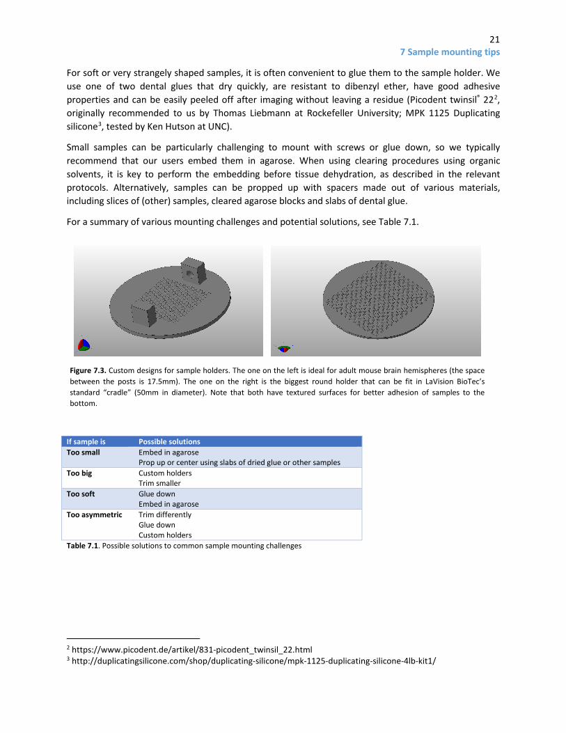
Figure 7.3. Custom designs for sample holders. The one on the left is ideal for adult mouse brain hemispheres (the space between the posts is 17.5mm). The one on the right is the biggest round holder that can be fit in LaVision BioTec’s standard “cradle” (50mm in diameter). Note that both have textured surfaces for better adhesion of samples to the bottom.

22 8 Optimizing imaging parameters

8 Optimizing imaging parameters 8.1 Introduction As in any imaging project, before starting any comprehensive optimization, there has to be a clear goal: what is going to be visualized and/or measured? Is the objective a visually appealing movie of an organ spinning in 3D? Is the goal to accurately count the number of cells of a certain type in a large sample? Does the project require tracing of filamentous networks or tree-like structures? These different goals have very different imaging requirements. In my experience, many labs are still trying to get a feel for this relatively new technology, and specific goals for datasets produced with the UltraMicroscope II may not be so clear, at least at first. Having said that, the optimization will be much easier once there are clear experimental objectives. In addition to having well-defined research goals, samples must be well-cleared and well-labeled; optimization cannot compensate for a poor sample.

The basic tradeoff when optimizing parameters is between time and quality, as is typical in many forms of microscopy. The latter is a term I will use loosely, but roughly includes XYZ resolution, signal-to-noise ratio of the fluorescent labels, and “evenness” of those two across the entire field of view. The goal during the optimization process is to obtain a dataset with the quality needed to answer the biological question in the least amount of time. The goal is not to obtain a 3D image with the highest possible resolution over the largest possible area. A need for higher resolution can result in much larger datasets, which will take longer to acquire and pose challenges for data management, visualization and analysis. Thus, it is not advisable to “max out” acquisition settings for high resolution, unless absolutely necessary. The key questions a user needs to answer in order to decide on settings are:

• What is the average spacing of the objects of interest? • How big is the total area of interest? • How important is it that the quality be even across the field of view?

In my experience, a new user of the system typically overestimates the required imaging quality and sample volume needed to answer their question, and is unaware of the importance of maintaining even quality throughout (as this is very salient in light sheet microscopy of large samples, but less so in more widespread imaging modalities like confocal and widefield microscopy).

In what follows, I will describe important light sheet parameters and how to adjust them optimally, explore other critical imaging factors and end with a recommended workflow and some examples.


8.2 Light sheet parameters and how to adjust them optimally 8.2.1 Light sheet width This parameter controls the power profile of the sheet along the Y dimension. The sheet is generated such that its intensity is roughly a Gaussian curve along the Y dimension; the width parameter in the software allows a user to control the shape of this curve. At lower widths the laser power is concentrated in the middle. At larger widths, power is distributed more evenly across the field of view and power density is lower.

The optimal width will depend on the size of the sample, the magnification and whether a single sheet or three sheets are used from a given side (Figure 8.1; see a detailed explanation of using one or three sheets (8.2.3)).

If laser power is not limiting, it is usually best to err on the side of larger widths to keep the illumination as even as possible. This is particularly important for accurate quantification of fluorescence intensity. However, if the width is too large, structures that are outside the field of view can cast shadows and are bleached unnecessarily. If laser power is limiting, widths that are too large will lead to exposures that are longer than they need to be. At very low magnifications, there will be significant unevenness in the illumination intensity along the Y dimension, even when using high width settings (for example, at 1.26X magnification, using three sheets, intensity is 31% higher in the center at 100% sheet width, Fig 8.2.C). We recommend using the minimal sheet width (given a magnification and number of light sheets) that leads to a difference in intensity between the middle and the edge of the sample smaller than 10%. The information in Fig. 8.2 can help make informed decisions about optimal sheet widths under different conditions. For example, using three sheets and 4X magnification, a minimum sheet width of 80% is needed to keep the intensity in the center of the field of view similar to the intensity at the edge of the field of view in the Y dimension.

Figure 8.1. Interactions between sheet width, number of sheets and size of the field of view (inversely related to magnification). Larger sheet widths lead to a more uniform distribution of laser power across the Y dimension in the field of view. Small fields of view (pink, typically with high magnification and/or cropping) have a more uniform distribution of power across the Y dimension in the field of view than large fields of view (black, typically with lower magnification and no cropping). Laser intensity is more evenly distributed when using three sheets instead of one.


Figure 8.2. (A) Schematic representation of measurements of excitation laser intensity distribution in the Y dimension. (B) Graphs show line profiles of light sheet power from the middle to the edge of the field of view at 1.26X magnification, for varying sheet widths and numbers of sheets (left: 3 sheets, right: 1 sheet), for the full field of view of the camera. The left graph in each group has the power normalized to the peak intensity of the 20% width light sheet; the right graph in each group normalizes the power to the peak at each width. (C) Tables show the ratio of the light sheet intensity in the middle compared to the edge of the field of view for different magnifications, number of sheets (left: 3 sheets, right: 1 sheet) and widths, for the full field of view of the camera. Lower ratios (more even illumination) are marked in blue and higher ratios (power strongly concentrated in the middle) are marked in red. As can be seen from these results, 3 sheets lead to more even illumination in Y, as does increasing the width of the sheet or imaging at higher magnifications. Measurements were made using the alignment tool provided by LaVision BioTec, which has a uniform solution of fluorophore inside.


8.2.2 Sheet NA and its effect on the shape of the light sheet in Z A major constraint on the quality of the imaging is the shape of the light sheet in the Z dimension. The sheet has a thin “waist” where the Z thickness is minimal and increases in thickness along the X dimension from there. The light sheet in this microscope is well described by the following model (Uwe Schröer, LaVision BioTec, personal communication):

𝑤𝑤(𝑥𝑥) = 𝑤𝑤0�1 + � 𝑥𝑥𝑥𝑥𝑅𝑅�2

(1)

where w0 is the beam waist, the half-thickness of the beam in the Z dimension at its narrowest, and x is the distance from the beam waist in the X dimension (Fig. 8.3).

xR (also called the Rayleigh length) is given by:

𝑥𝑥𝑅𝑅 = 𝜋𝜋𝑤𝑤02

𝜆𝜆 (2)

where λ is the wavelength of the light sheet. Note that the Rayleigh length (xR) is the distance from the waist at which the beam thickness in Z has increased by around 40%. Double this length (2. xR = b, Fig 8.3) is frequently used to estimate the region over which the light sheet is “flat” in the Z dimension. This is shown graphically by the LaVision BioTec software as a bowtie shape in the image preview window (I adopt the same convention in Figs. 8.12).

The beam waist w0 can be calculated from:

𝑤𝑤0 = 𝑅𝑅𝑅𝑅.𝜆𝜆𝜋𝜋.𝑁𝑁𝑁𝑁

(3)

where RI is the refractive index of the immersion fluid and NA is the numerical aperture of the light sheet generating optics. For example, using the RI of dibenzyl ether (1.56), 647 nm (our most commonly used laser excitation line) and 0.155 (the highest possible light sheet NA setting on our UltraMicroscope II), w0 is 2.07 µm. Therefore, under those conditions, the full thickness of the sheet at its narrowest (2w0) is 4.14 µm.

Figure 8.3. Important light sheet shape parameters, assuming a single sheet propagating from right to left in the X dimension. The origin is set to the center of the sheet in X and Z and, unless stated otherwise, the horizontal focus of the sheet is centered in the field of view.

+X

w(x)

2� w0 w0

xR

b=2.xR

+Z

(0,0) -X

-Z


From equations (1)-(3), it is clear that the thickness of the sheet at its thinnest is set by the numerical aperture (NA) of the optics that generate it. A higher NA will result in a higher Z resolution over a smaller region (shorter Rayleigh length) whereas a lower NA will result in a lower Z resolution that does not deteriorate as quickly from the waist (longer Rayleigh length). The way the system lowers the NA is by decreasing the size of an aperture that blocks the laser, so the lower the NA, the lower the intensity of the sheet (Fig. 8.4).

Since the light sheet shape is generated independently of the image collection optics, the non-uniformity of the light sheet thickness in the Z dimension is much more noticeable at lower magnification and/or without cropping, compared to higher magnification and/or with cropping (because more regions of the sheet farther from the waist fall into the field of view; Fig. 8.5).

Figure 8.5. Illustration of the effects of changing the magnification and/or cropping.

Figure 8.4. The effect of modifying light sheet NA. These sheets were created assuming RI = 1.56 (dibenzyl ether), λ = 647 nm, NA = 0.154 (high) or NA = 0.034 (low) using equations (1)-(3). The field of view shown here corresponds to 12.6X total magnification (approximately 1000 µm wide in the X dimension).

x

z

High NA sheetTighter sheet waistUneven Z resolution across field of viewBrighter

Low NA sheetBroader sheet waistMore even Z resolution across field of viewDimmer


8.2.3 Number of sheets: three vs. one By default, the system illuminates the sample with three sheets that are slightly angled (at around 11 degrees from horizontal in the UNC system). This allows visualization “behind” portions of the sample that interfere with light propagation (areas that are not well cleared, bubbles, etc.; Fig. 8.6).

The advantage of using three sheets comes at a cost in Z resolution. The reason is that the waists of the three sheets can only be aligned to each other in the center of the field of view. Thus, when the three sheets are combined, one of them will be wider in Z than a single sheet at most positions in the field of view (Fig. 8.7). This is true even if the system is perfectly aligned. Thus, to obtain the best possible Z resolution across the entire field of view, it is necessary to use a single sheet. When using a single sheet, the power in the sheet will be lower (in the UNC system, around 60% of the power is in the central beam) so laser power will need to be adjusted to compensate, or longer exposures will be required to obtain the same quality. Additionally, striping artifacts, which are common in samples that are not perfectly cleared, will become more prominent when using a single sheet (Fig. 8.6). Having said that, it is easier to computationally remove striping artifacts from one sheet, rather than three (though, see Liang et al, 2016).

Figure 8.6. Shadowing and striping artifacts expected with three sheets (left) or one (right). Note that illumination with a single sheet causes stronger shadowing behind structures that block light propagation. The diagram assumes the red structure completely blocks light propagation. Shadowing intensity is based on relative power levels between sheets observed on the UNC system (55% in central sheet, 32% in top sheet and 13% in bottom sheet, with lateral sheets angled at 11 degrees from horizontal; this can vary between microscopes). For the single sheet case, it assumes the laser power has been increased so that the total illumination intensity is the same as in the three sheet case.


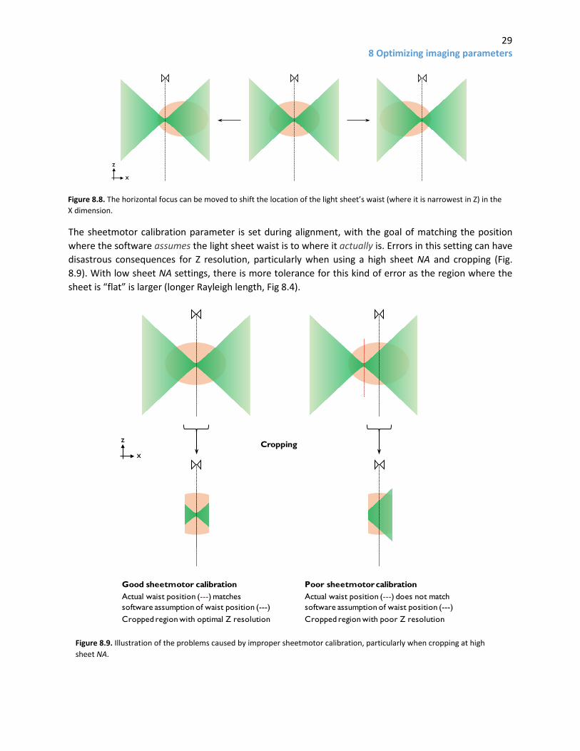
8.2.4 Horizontal focus and sheetmotor calibration– positioning the sheet waist In addition to modulating the sheet NA and the number of sheets, the user can adjust the location of the horizontal focus (the waist of the sheet) in the sample, to ensure particular features are imaged with the highest possible Z resolution (Fig. 8.8). There is also the option to take images with the horizontal focus at different positions in X, and then merge them together using one of various algorithms (described in the dynamic focus section (8.3.5)).

Figure 8.7. Modeling showing the detrimental effect on Z resolution of using three light sheets instead of one. The model uses equations (1) and (2), assuming 647 nm laser excitation, 5 µm light sheet thickness, 1.3X magnification, horizontal focus of all three sheets centered in the middle of the field of view, oblique light sheet angles of 10.6 and -10.1 degrees (these are the values for the UNC system), and no radial aberrations of the objective (which can be significant near the edges at low magnification). The graphs show the expected thickness of the sheet at different locations in the field of view, relative to the minimal (5 µm) width in the center of the field for each sheet (top panels) or the combination of all three (bottom panel). In the case of multiple light sheets, the width of the illumination in Z was taken as the widest of the three options. While this simplified model does not weigh the effect of the different light sheet intensities and does not incorporate any kind of interference effects, it illustrates that adding the two angled sheets to the one in the middle decreases Z resolution everywhere except the very center of the field of view. See also Fig. 8.12 for measurements that show this in a sample.


The sheetmotor calibration parameter is set during alignment, with the goal of matching the position where the software assumes the light sheet waist is to where it actually is. Errors in this setting can have disastrous consequences for Z resolution, particularly when using a high sheet NA and cropping (Fig. 8.9). With low sheet NA settings, there is more tolerance for this kind of error as the region where the sheet is “flat” is larger (longer Rayleigh length, Fig 8.4).

Figure 8.8. The horizontal focus can be moved to shift the location of the light sheet’s waist (where it is narrowest in Z) in the X dimension.

x

z

Figure 8.9. Illustration of the problems caused by improper sheetmotor calibration, particularly when cropping at high sheet NA.

x

z

Good sheetmotor calibrationActual waist position (---) matchessoftware assumption of waist position (---)Cropped region with optimal Z resolution

Cropping

Poor sheetmotorcalibrationActual waist position (---) does not matchsoftware assumption of waist position (---)Cropped region with poor Z resolution


8.2.5 Laser power There are two ways of controlling laser power on the UltraMicroscope II, and depending on the exact configuration, a system can be equipped with one of them or both.

The first is by using the slider labeled “laser power” in the software. This software slider controls the position of a single mechanical wheel with a continuous neutral density (ND) filter, positioned in the microscope after all lasers are combined in the light path. Changes in the laser power setting cause wheel movements that place a different section of the ND filter (with different attenuation properties) in front of the laser beam. A big disadvantage with this way of controlling laser power is that it can slow down multichannel acquisitions if the power settings vary between channels and the channels are switched at every Z position (as the single, slow wheel needs to move back and forth at every Z plane). Another issue with controlling the power in this manner is that the software incorrectly expresses laser power as a percentage. However, this percentage refers to movement of the mechanical wheel, while the actual ND filter on the wheel attenuates laser power exponentially. For example, 80% power is 40 times higher than 10% power, not 8 times higher, as expected if it were linear. Thus, precise determination of power levels requires measurements with a power meter (see power curve for the system at UNC, Fig. 8.10). Since the information in this power curve can be used to speed up image acquisition (see below), precise measurements of laser power are very useful for routine operation.

The second way of controlling laser power is—in systems with more than one laser—at the laser heads themselves, through an independent menu in the software. This depends on the exact setup of the system, but if this control mode is available, it is much faster for multidimensional acquisition as it does not require any movement of the attenuation wheel. The only problem with this way of controlling the laser power is that the software does not revert to a default power setting upon closing. Thus, in a multi-user environment, users must be vigilant and check the laser settings upon startup, to ensure they are appropriate.

Figure 8.10. Actual (measured) laser power as a function of the “laser power” software slider position. Note the logarithmic scale for measured laser power. Measurements shown for the 647 nm laser on the UNC system, but curves are very similar for other laser lines.


The optimal power level for imaging is usually not the optimal power level for exploring the sample and setting up other conditions. When a user is exploring the sample, they will frequently pause, adjust the settings and typically spend much more time at each plane than they would during imaging. Thus, using high laser power and low exposure during exploration will cause bleaching. This bleaching can be seen in a 3D representation of the final stack of images as a thin dark shadow (which looks like a cut that is thinner in the middle) in an XZ or YZ view of the sample. Circumventing this problem is simple: while exploring, avoid high laser powers and instead use long exposures (Table 8.1). During the exploration and optimization phase, the user can adjust the exposure (and only the exposure) for an optimal signal-to-noise ratio. Before starting the actual imaging run, the power curve can be used to calculate how much the exposure can be lowered by increasing the laser power. In tests using the system at UNC, there are speed improvements when lowering the exposure down to 10 ms; shorter exposures provide no further speed benefit. For example, if an exposure of 400 ms and 10% power gave good results, imaging for 10 ms with 40 times more power would give results of equivalent quality. Because of the non-linear nature of the attenuation wheel, 40 times more power is achieved (on the UNC system) at the 80% power setting (Fig. 8.10). Opting for these power and exposure settings during an imaging run with a single channel and 2000 Z positions would save 13 minutes (compared to 400 ms with 10% power).

Table 8.1. Laser power recommendations for exploring samples vs acquiring data. Some representative power levels and exposure times from the UNC system are provided.


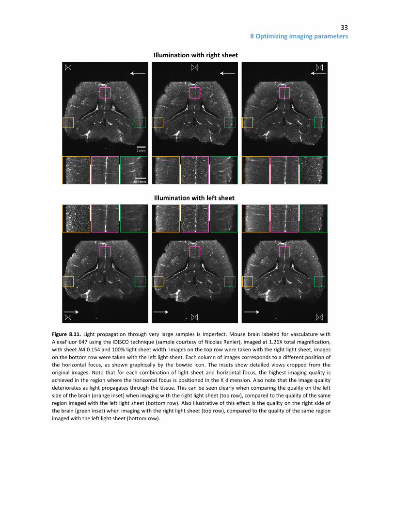
8.3 Additional imaging considerations 8.3.1 Imperfect light propagation through samples - imaging from both sides A common limitation to successful imaging is imperfect light propagation through the sample. This is usually not a big problem in well cleared, narrow samples, when using long wavelengths (red or higher). However, if samples are very wide and/or haven’t been cleared properly, and/or are being imaged in the green (or shorter wavelength) channel, the side farthest from where the light sheet enters the sample can look worse, even if the light sheet’s horizontal focus is placed there (Fig. 8.11). If this occurs, a possible solution is to use light sheets from both sides, sequentially, at the cost of more imaging time and photobleaching.

The increase in imaging time when using the left and right sheets is substantial, not just a two-fold increase; changing the side from which the sample is illuminated requires movement of a mirror on a mechanical arm, which is comparatively slow. For example, on the system at UNC, using both sheets adds (in addition to the doubled exposure time) approximately 0.26 s of imaging time per image. Assuming a stack with 2000 images (5 mm in Z at 2.5 µm spacing), each of which has a 10 ms exposure, using both sheets adds almost 9 more minutes of imaging time, of which only 20 seconds are additional exposure time and the rest is due to mechanical movements.

When imaging using both light sheets, the software has three options for blending the two images into one. The simplest is to use a blending algorithm. This generates the left side of the final image from the image taken with the left light sheet, the right side of the final image with the image taken with the right light sheet, and does a linear interpolation to blend things in the middle of the image (how wide the interpolation region is can be controlled in the software). Alternatively, there is a contrast enhancement mode which looks at various vertical stripes of the left and right side image, and includes the one with best contrast in the final image. The details of how this algorithm works are not clearly explained by LaVision BioTec’s documentation. A scenario in which this algorithm may be convenient is if the sample has a light-altering imperfection near one side (for example, a bubble). In that case, the simple blend mode would likely generate an image with considerable shadowing “behind” the imperfection, whereas the contrast mode might give a better result (by using the opposite light sheet over a wider region than the blend mode). Finally, the system offers a maximum projection option, which typically gives very poor results and should be avoided.

An important consideration when using two sheets is where to place the light sheet waist. A good option is usually to place it halfway between the middle of the sample and the furthest edge of the sample in the direction of the incident light sheet (this is the approach I took in the dataset in Figure 8.12.C). Placing it in the middle “wastes” part of the region with a thin Z (since it will be blended out) whereas putting it in the middle of a hemisphere of the image may not be appropriate if the sample does not cover the entire field. Alternatively, the waist on each side can be placed to optimize the Z resolution of features of interest.

When using two sheets, it is critical for the left and right sheets to be aligned in the Z dimension, and to be of similar intensity. If not, the blending will generate images that are of different Z positions of the tissue on each side, and/or have different intensities. This can be easily checked and adjusted during alignment of the system with an alignment tool provided by LaVision BioTec.


Figure 8.11. Light propagation through very large samples is imperfect. Mouse brain labeled for vasculature with AlexaFluor 647 using the iDISCO technique (sample courtesy of Nicolas Renier), imaged at 1.26X total magnification, with sheet NA 0.154 and 100% light sheet width. Images on the top row were taken with the right light sheet, images on the bottom row were taken with the left light sheet. Each column of images corresponds to a different position of the horizontal focus, as shown graphically by the bowtie icon. The insets show detailed views cropped from the original images. Note that for each combination of light sheet and horizontal focus, the highest imaging quality is achieved in the region where the horizontal focus is positioned in the X dimension. Also note that the image quality deteriorates as light propagates through the tissue. This can be seen clearly when comparing the quality on the left side of the brain (orange inset) when imaging with the right light sheet (top row), compared to the quality of the same region imaged with the left light sheet (bottom row). Also illustrative of this effect is the quality on the right side of the brain (green inset) when imaging with the right light sheet (top row), compared to the quality of the same region imaged with the left light sheet (bottom row).


8.3.2 Radial aberrations in the optics Aberrations around the edges of the field of view that distort the image and lead to low signal intensity are another challenge when imaging with this system. These radial distortions are due to the imaging optics, get worse as the distance from the center of the field of view increases, and are particularly prominent at lower magnifications with the zoom optics configuration.

In XY views, the effect of these aberrations can easily be seen at low magnification by moving a sample with distinct features to a corner of the field of view, while imaging with a single light sheet from one side and placing the horizontal focus on the edge of the field of view (to ensure no distortions are due to increased sheet thickness far from the sheet waist or the combination of 3 sheets, Figs. 8.5 and 8.7). Under those circumstances features in the corner will look dimmer and blurrier than if they were closer to the center of the field of view (with the horizontal focus also in the center).

These aberrations can also be visualized with a YZ projection of image stacks taken with a single sheet from one side centered—in X—at the position of the horizontal focus of the light sheet (this will eliminate any distortions due to increased sheet thickness). As this measurement is repeated with the horizontal focus closer to the edge of the field of view, image quality at large distances from the center of the field of view (in Y) will deteriorate.

These XY and YZ views can be used to determine whether cropping is warranted given the level of distortion and the analysis that will be performed, and if so, how much cropping is needed (see cropping section (8.3.3)).

These aberrations are dramatically worse using the non-corrected dipping caps for the zoom optics, which is why those caps should be avoided in almost all circumstances (the possible exception being samples where a working distance greater than 5.7 mm is an absolute necessity, in which case the 10 mm working distance cap can be used instead of the corrected dipping cap). Unfortunately, I have not yet mapped these aberrations precisely, which will require samples with subresolution fluorescent beads embedded in blocks of cleared agarose. As a result, I cannot provide systematic guidelines for how much to crop to avoid these aberrations under various imaging conditions.

While these aberrations are smaller with the infinity optics, LaVision BioTec does not provide detailed information on this point and I do not have precise measurements showing how much the infinity optics ameliorate this problem.

8.3.3 Cropping Cropping is often useful on the UltraMicroscope II, because of the large default file sizes (around 10 MB), as well as the fact that most problems with image quality occur on the edges of the field of view in the X and Y dimensions.

If the sample does not fill the entire field of view, cropping will reduce the size of the dataset with no downside. Smaller datasets will transfer more quickly between computers, can be saved faster, and do not use as many computational resources when they are analyzed.

By cropping the image in the X dimension, a more even Z resolution can be ensured, as cropping will remove regions where the light sheet is thicker in the Z dimension, particularly at high sheet NA values


(Fig. 8.5). By cropping the image in the Y dimension, the field of view can be restricted to a region where the power variation in Y (Fig. 8.2) is within acceptable limits, which is a concern at lower magnifications and sheet widths. Cropping in both dimensions also helps avoid some of the optical aberrations that affect the edges of the field of view, particularly at low magnifications (see radial aberrations section (8.3.2)), as well as restricting the imaging to a region with lower combined light sheet thickness when using 3 sheets (see number of sheets section (8.2.3), and Fig. 8.7).

When imaging from a single side and using cropping, the sheetmotor calibration has to be set properly, the light sheet needs to be centered in the middle of the—uncropped—field of view and the cropping region needs to be centered as well. If there is any deviation from these conditions, the cropped field will not have the waist of the sheet in the middle and the Z resolution will be worse, dramatically so at high sheet NAs (Fig. 8.9).

If cropping is used to enhance the quality of the imaging, as described above, but the sample size is such that it does not fit in the cropped region, tiling of multiple images at different XY locations will be needed (see tiling section (8.3.4)). The software supports automatic tiling of cropped regions.

8.3.4 Tiling Tiling is often required in large samples, when imaging at high magnification, when cropping, or when a combination of all of those conditions occurs.

The key when tiling is to ensure sufficient overlap of high quality information on the edges of images. This allows subsequent stitching to work properly. Given that the major problems with image quality occur on the edges of images (due to radial aberrations in objectives and thicker widths of the sheet in the Z dimension), this presents a problem. The best solution is usually to crop the image down to a size that minimizes aberrations on the edges, and to tile using a small overlap percentage of these—higher quality—edges. We have been successful with overlap values as low as 10% in regions cropped in the center of the field of view, though this will depend on the sample and exact acquisition conditions. LaVision BioTec supports Terastitcher (Bria et al, 2012) for stitching downstream of tiling, and commercial options for stitching are also available (for example, the Bitplane Imaris Stitcher has a simple workflow and has given us good results in many—though not all—samples).

If tiling is to be combined with left and right sheet imaging, this presents a challenge. While the software supports blending of left and right images under these circumstances, it only applies the desired blending after all the tiles have been acquired with both sheets. For example, if a 3x3 tile were acquired, the final result can be blended such that the left column comes from images taken with the left light sheet, the right column comes from images taken with the right light sheet and the middle column from a linear interpolation of images taken with right and left sheets. However, the software implementation is such that it will acquire two images (using left and right light sheet) at every tiling position and then throw away data or combine it as desired. This represents an obvious waste of time (acquiring images that will not be used in the final result) and an inefficient use of the bleaching budget (acquiring images that will lead to bleaching but not contribute any useful information to the final dataset). While there are manual workarounds to this problem with the software setup, there is currently no way to easily set which tiles are to be imaged with which light sheets.


8.3.5 Using the dynamic focus When images of high resolution across large areas are required, an option is to use dynamic focusing. Instead of keeping the light sheet in one location and moving the sample to tile, this keeps the sample in one place, and moves the horizontal focus position of the sheet throughout the sample (Fig. 8.8). Multiple images are acquired and then blended together to ensure maximal Z resolution across the entire field of view. How many images are needed for this to work depends on the magnification (fewer at high magnification), the NA of the sheets (more at high NA), and the size of the region over which this sweeping of the horizontal focus is to occur (which is set by the user, is typically from edge to edge—in X—of the sample and is directly proportional to how many images will be taken). The software recommends a number of images, which, according to LaVision BioTec, tends to be an overestimate (how much of an overestimate is unclear, and requires testing in each sample).

The software offers two blending algorithms: blend and contrast enhanced. These are not explained in detail in LaVision BioTec’s documentation but operate roughly as follows. Blend takes vertical stripes where the software predicts the horizontal focus of each image will be and then blends the edges of these together, analogous to how the blend algorithm for the left and right sheet works. For blend to work correctly, it is absolutely critical that the sheetmotor calibration be perfect. If that is not the case, there will be a mismatch between where the blending algorithm assumes the sheet waist will be and where it actually is, giving very poor results (Fig. 8.9). To circumvent this problem, the blend algorithm has a calibration option where the system will take a small stack, use it to determine where the sheet waist is at different horizontal focus positions and then apply the algorithm based on this measurement. In our tests at UNC, we have only had mixed success with this algorithm. An alternative is the contrast enhanced algorithm. This algorithm does not assume anything about where the light sheet waist is, and selects the vertical stripes with the best contrast (with “contrast” defined in a way that has not been explicitly documented by LaVision BioTec) from all of the acquired images. We have noticed that both algorithms can have problems and smear images in the Z dimension when exposures are lower than 100 ms, which can make dynamic focusing even slower than it already is. This seems like a bug in the software; LaVision BioTec has been informed of it and is working on a solution.

The optimal approach when using the dynamic focus will be highly sample dependent and should be tested extensively. This will help determine the optimal NA and magnification of the sheet for the question at hand, the optimal number of images for the dynamic focus and the best algorithm. As explained in section 8.2.3, and seen in Fig. 8.7, a single sheet will perform better than three sheets if maximal Z resolution across the entire field of view is required. Fig 8.12.D and E illustrate use of the dynamic focus with one or three sheets in a real sample.

8.3.6 Acquiring multi-channel images When more than one channel will be acquired, additional issues need to be taken into account.

During exploration of samples labeled with multiple fluorophores with different bleaching characteristics, it is a good idea to set up as many imaging parameters as possible in channels with more tolerance to bleaching. While all channels need to be evaluated, looking at particularly sensitive fluorophores only when absolutely necessary will minimize their bleaching before data is acquired.


Critically, images of different fluorescent channels will not be focused at exactly the same position in the detection path of the system, due to chromatic aberrations in the lenses. The difference between the channels is more noticeable at higher magnifications, and is larger the farther apart their wavelengths. To compensate for this, LaVision BioTec includes a chromatic correction module with a moveable lens which can shift different distances for different channels, such that they can all be focused in the same plane on the camera chip. The time it takes to make this shift is significant, particularly at high magnifications when excitation wavelengths are very far apart (example: 488 nm and 647 nm). Another issue with the chromatic correction module is that LaVision BioTec’s original design is such that the correction cannot compensate between 647 nm and 488 nm excitation at the highest zoom option (6.3X) in the zoom body configuration of the microscope. A new chromatic correction module that can extend over the entire zoom range became available in mid-2018.

Image acquisition can also be slowed down by the need to change emission filters (and excitation filters, if using the white light laser) when switching between channels. The system configuration with individual laser lines can be coupled to a dual (or multi) emission filter to avoid this mechanical movement, thus speeding up the acquisition (at the expense of potential cross talk).

Different channels may have different signal intensities and require their own optimal combination of laser power and exposure time. Unfortunately, the software does not allow different exposure times for different channels. Thus, laser powers need to be adjusted for each channel to optimize their signal to noise. As described in the laser power section (8.2.5), there are two ways of doing this: at the laser head (faster, only possible if the system has individual lasers) or through the attenuation wheel (slower). Movement of the attenuation wheel can introduce delays if channels require very different laser powers to have comparable signal-to-noise.

Once basic conditions have been decided on, a decision has to be made with respect to the acquisition order of a multichannel Z stack: Z then channels, or channels then Z. Switching between channels many times in the channels then Z configuration significantly slows down the acquisition, since it usually requires mechanical movement of relatively slow components like the chromatic correction lens, filter wheels and the power attenuation wheel (see above). Thus, the Z then channels configuration is much faster than channels then Z. However, doing Z then channels may lead to misalignments between channels due to small sample movements, or slight drifts of the motorized stage. Channels then Z may be the better acquisition configuration when the goal is to perform precise spatial comparisons between channels. This is something that is worth testing, because if the alignment between channels is acceptable with the Z then channels acquisition order (or easily correctable computationally post hoc), imaging will be much faster.

In summary, taking images with multiple channels can be significantly slower than the sum of all the exposure times, particularly with channels spaced far apart in the spectrum, at high magnification and with a channels then Z acquisition order.


8.4 Workflow summary and examples I suggest that researchers start by adjusting the magnification, on the basis of the required XY resolution to discern objects, which depends on the spacing of those objects (though not necessarily their size). If the desired view of the sample exceeds the field of view, this means that tiling will be required. Once the magnification has been adjusted, the sheet width can be set to avoid uneven illumination along the Y dimension (Fig. 8.2). After establishing this baseline, the conditions with which each image will be acquired will depend on the desired Z resolution, and the desired evenness of that Z resolution across the field of view.

As explained in the preceding sections, sheet NA (Fig. 8.4), number of illuminating sheets (Figs. 8.6, 8.7), horizontal focus (Fig. 8.8), side(s) of illuminating sheets, cropping (Fig. 8.5) and dynamic focus will need to be evaluated. During exploration of the sample, the exposure time can be set to obtain the desired signal-to-noise ratio in the image. For actual imaging runs, laser power can be traded for exposure time to obtain the same signal-to-noise ratio in the image while ensuring faster acquisition, as described in the laser power section (using Fig. 8.10).

Given the large number of parameters that can be adjusted, it is useful to test different options before deciding on the optimal imaging conditions. A good test is to acquire relatively small (100-1000 µm) Z stacks of samples, ideally in regions with relatively even staining throughout the sample, using a small Z spacing (2 µm is a good choice). A very useful tool when comparing conditions is an orthogonal projection, particularly in the XZ dimension, as this is the projection that allows an easy visual representation of the Z resolution across the field of view. XZ projections at different Y positions can help evaluate the effect of the number of illuminating sheets and radial aberrations (YZ projections can also be useful for this). Examples of different imaging conditions are shown in Fig. 8.12.

By comparing the resulting quality and time to image among various other options, a user can determine which imaging conditions provide the best tradeoff between quality and time for their particular sample and biological question. By subsampling the data in the Z dimension, users can determine whether 2 µm spacing is required, or whether larger intervals are sufficient (reducing imaging time and bleaching).

This general approach to optimization can lead to very different imaging conditions, depending on the exact experimental needs.

On one extreme, a user might want a good quality view of a single vertical strip in the sample, and a lower quality view of the rest of the sample would suffice. An example of this would be an embryo with labeling of interest concentrated in its spinal cord. In this case, it might be convenient to orient the sample with the spinal cord towards one side, set the horizontal focus there with a relatively high sheet NA, and image at a low enough magnification to quickly capture the entire embryo in a single Z-stack.

If Z resolution is not critical but a more even (with respect to quality in Z) view of the sample is preferable, the fastest way to accomplish this is by lowering the sheet NA. If the laser power can be increased to compensate for the lower power density of the low NA sheet, this will not increase the imaging time. The final image will have a more even Z resolution across the X dimension, though that resolution will be lower in the center compared to a case where a higher sheet NA was used (Fig. 8.4). If the image of the sample looks worse on the far side of the incident light sheet, this suggests there are problems with light propagating through the sample, and a good approach is to use two light sheets.


If resolution is critical, but only a small sample region needs to be imaged, the best balance is usually achieved by taking an image at high magnification (to ensure high XY resolution) with the sheet set to a high NA (to ensure high Z resolution). To guarantee the resolution in Z is as high as possible across the entire field of view, it is critical to only use a single light sheet for illumination, turning off illumination with the two angled sheets. When using a single sheet, the power in the sheet will be lower (in the UNC system, around 60% of the power is in the central beam), so laser power will need to be adjusted to compensate, or longer exposures will be required to obtain the same quality. Additionally, when using a single sheet, structures that interfere with light propagation (typically due to poor clearing of the sample, or bubbles) will be much more noticeable, but this is usually a worthy tradeoff to make if the objective is to maximize the resolution.

The most complicated scenarios are those in which high resolution is required over a large field of view. This requires extensive tiling of cropped regions using high sheet NA, dynamic focusing, imaging with light sheets from both sides, or a combination of all of these.

Ultimately, these are only general guidelines; the best way to determine the optimal settings is to perform small pilot tests, check the quality of the results against what is needed for the desired analysis and determine if the price in imaging time (and bleaching) are tolerable. I present a summary of the typical workflow for parameter optimization in Table 8.2.

Parameter Influenced by 1. Magnification Spacing of objects of interest in sample 2. Sheet width Magnification

Sample size Cropping

3. Sheet NA Spacing of objects of interest in sample Need for evenness in Z resolution across the X dimension

4. Number of sheets on each side: 1 vs 3 Spacing of objects of interest in sample 5. Laser power/exposure Quality of fluorescence labeling

Desired signal-to-noise for analysis/visualization Presence of multiple channels Sheet NA Number of sheets Sheet width

6. Left and right light sheets Sample transparency Size of sample Need for evenness in quality and illumination across the X dimension

7. Cropping Sample size Radial aberrations (dependent on magnification) Tiling

8. Tiling Sample size Magnification Sheet NA Radial aberrations Cropping

9. Dynamic focus Sample size Magnification Sheet NA Need for evenness in Z resolution across the X dimension

10. Multiple channels Number of fluorophores in sample Table 8.2. Workflow for parameter optimization. List of parameters that need to be optimized, factors that influence each parameter and the rough order in which to optimize them.


Figure 8.12. (see next page for figure legend).


Figure 8.12 (continued, see previous page for figure). Examples of XY (top) and XZ (bottom) views of the same sample, acquired with different conditions. The sample is the one in Fig. 8.11: a mouse brain labeled for brain vasculature with AlexaFluor 647 (sample courtesy of Nicolas Renier). All imaging in this figure was performed at 4X total magnification, with 100% sheet width, taking a 100 µm Z stack at 2 µm spacing, using the zoom optics configuration of the UltraMicroscope II. 100 ms exposure was used in (A)-(C), and 100.485 ms in (D)-(E)--which was the closest option to 100 ms offered by the software when doing dynamic focusing. NA of sheets, number of illuminating sheets, side and horizontal focus position of illuminating sheets and dynamic focusing are as indicated for each dataset. For each condition, the relative time it took to acquire the stack is indicated (1x=12 s). Brightness and contrast were adjusted to show visually similar intensities in the figure (without these adjustments, lower NA conditions have lower intensity). The XZ projections are taken within the colored boxed regions shown in the top row and constitute a maximum projection along the Y axis over a 36 µm span. XZ projections are enlarged roughly 4.6-fold relative to XY views (see scale bar) and image gamma was modified in FIJI to 0.6, to enhance the display of dim, small features. The five imaging conditions were selected to illustrate the effects of various key parameters on image quality, particularly in the Z dimension. An NA of 0.154 (sheet waist ∼5 µm) using 3 sheets from the right (A) shows excellent resolution in the center of the field of view that deteriorates rapidly towards the edges (in the X dimension, see XZ projection). An NA of 0.017 (sheet waist ∼ 43 µm) using 3 sheets from the right (B) leads to considerably worse resolution in Z but the quality remains more even along the X dimension. A sheet NA of 0.017 was selected because the light sheet’s thickness in Z changes by less than 40% across the entire field of view at this magnification. Imaging with the right and left sheets (C) was performed with an NA of 0.026 (sheet waist ∼ 28 µm), with the horizontal focus centered on each of the respective halves of the image, and using blend mode to combine them. The 0.026 sheet NA was selected because this kept the light sheet Z thickness on each side of the image from changing by more than 40%. The doubling in acquisition time when using the right and left sheets gives better Z resolution than (B), and is even along the X dimension. As expected from the lower NA, Z resolution in the very center of the field of view is worse than in (A). Both conditions using the dynamic focusing used an NA of 0.154, 25 positions (the software recommended value) spanning the entire width of the field at this magnification, and the contrast adaptive blending algorithm. Laser power was increased in the single sheet condition (E) to compensate for the absence of the two tilted sheets. For the dynamic focus conditions two XZ projections are shown: centered in the middle—in Y—of the field of view (purple) or at the very top (yellow). Note that the XZ projections in the middle of the field of view (purple) show that the Z resolution for both dynamic focus conditions is maximal and very even across the entire field of view (only slightly worse in the 3 sheet case at the very edges of the field of view). In contrast, at the very top of the field of view (yellow), the triple sheet case (D) is considerably worse than the single sheet case (E). This is as expected from Fig 8.7. Any remaining blurring or decrease in intensity at the edges of the field (for example in the corners) are likely due radial aberrations at this magnification. The significant increase in Z resolution across the entire field of view achieved with the dynamic focus comes with a big cost in acquisition time, which is an order of magnitude higher than the fastest options tested with this sample (A and B).

42 9 Alignment tips

9 Alignment tips

LaVision BioTec provides instructions and training on how to align the microscope using an alignment tool that comes with the system. I will not replicate those instructions here, but will make a few additional comments, based on our experience in the UNC Core.

During installation, I highly recommended that new users check the following (in addition to the standard alignment):

1. The waist of all three sheets on each side should be at the same position. This can only be modified on-site by LaVision BioTec using a special tool, so the time to ensure this is correct is during installation. If this is off, it will significantly degrade the Z resolution of the system when using more than one sheet (beyond what it is already degraded when using three perfectly aligned sheets instead of one, Fig. 8.7). If you notice that you can’t seem to get all three sheets looking sharp going through the alignment tool but you can fix one sheet that looks off by moving the sheetmotor calibration, the horizontal alignment of the waist of one of the sheets is off.

2. The left and right sheet should have very similar brightness across the entire range of sheet NAs. Because lowering the sheet NA closes an aperture, if this aperture is not calibrated properly, one of the sheets will be dimmer than the other. This will show up as one side being dimmer than the other in two-sided imaging conditions. While this can be fixed by LaVision BioTec remotely, it is better to check that everything looks good when the system is installed.

3. All lasers should be aligned to each other in Y, Z and in their horizontal focus. It is much easier to have LaVision BioTec check this during installation of the system than to try and fix it after the fact.

We at UNC check the alignment every week and frequently need to make adjustments. Based on my experience with the system, I would consider one week the maximum advisable interval between alignments. If high resolution work with high sheet NA combined with cropping (and/or dynamic focusing) is done frequently, it is critical to check the sheetmotor calibration before long runs. It is possible that this degree of instability in the alignment is particular to the UNC system and the environmental conditions of the room it is in. To be safe, however, I would recommend checking the alignment every week for the first few months after a system is installed, to gather baseline information on its stability. For reference, Table 9.1 has statistics of significant alignment adjustments at UNC that were needed over the course of 89 checks of the alignment (roughly once a week). Perhaps the most important value is the fraction of times the alignment was checked and a need for realignment was discovered: 80%. Clearly, weekly realignment of the UNC system is essential and, for some applications and periods of high usage, probably insufficient.

43 9 Alignment tips

Parameter requiring realignment Probability

Right side

Y central sheet 0.47

Sheetmotor 0.33

Z tilted sheets 0.16

Y tilted sheets 0.12

Left side

Y central sheet 0.39

Z central sheet 0.48

Sheetmotor 0.38

Z tilted sheets 0.18

Y tilted sheets 0.13

At least one parameter 0.80

Table 9.1. Summary of realignment statistics from the UNC system, based on 89 alignment checks performed approximately every week.

In addition to checking the alignment every week, we also perform the following maintenance tasks on the system:

1. Check dipping cap for scratches, leaks or cracks. 2. Change DBE in reservoir. 3. Check for DBE spills. 4. Check air table for proper operation. 5. Perform updates, virus scans and disk checks on computer, and clean hard drive to ensure at

least 1-2 TB for week’s experiments.

With this schedule of weekly maintenance and alignment, we have never had any major problems with the system.

44 10 Deconvolution

10 Deconvolution

Image restoration using deconvolution seems like a natural way to improve image quality, particularly as it refers to Z resolution. Unfortunately, there are a number of major challenges to implementing this successfully with the images from this microscope.

Many typical deconvolution algorithms assume spatial invariance of the point spread function (PSF) of the microscope, or only account for minimal variation of the PSF across the field of view. In contrast, in this system we know the point spread function will vary systematically in the X dimension as the light sheet increases in Z thickness from its waist (Fig. 8.3). This systematic variation needs to be accounted for in the deconvolution algorithm. Complicating things even more, the user can dynamically select between a multitude of sheet NAs (and therefore shapes), as well as a horizontal focus position optimal for their sample (Figs. 8.4, 8.8). If there are any misalignments of the sheetmotor calibration, the horizontal focus position that is assumed may not be the actual one, complicating things further (Fig. 8.9). This is all under the scenario of a single light sheet coming in from one side. Adding tilted light sheets, imaging from both sides and/or using the dynamic focus option will significantly increase the complexity of the deconvolution model required. As of this writing (September 2018), of the two major deconvolution software packages that I know of and have experience with, Autoquant cannot deal with these datasets very effectively and Huygens can improve upon the very simplest situation of a single well aligned light sheet from one side. LaVision BioTec is working on deconvolution algorithms based on the dynamic focusing.

Given the potential improvements that could result from using deconvolution on UltraMicroscope II datasets, this is an area that I consider ripe for major improvement in the—hopefully near or medium—future.

45 11 Data transfer

11 Data transfer Using the experience in the UNC Core as a case study

When acquiring large datasets, data transfer can be a rate-limiting step in the workflow, so it is beneficial to identify the potential problems, constraints and possible solutions.

11.1 Defining the problem Transferring data is slow. “Slow” is anything that annoys users of the microscope. In the UNC Core, users get annoyed when:

• Transferring data from an acquisition computer to an analysis workstation, network storage or external hard drive takes longer than 5 minutes.

• The core charges them for usage on an instrument when they are just transferring data.

11.2 Defining other problems that the UNC Core cannot solve quickly, cheaply or at all • Long-term storage and backup of data. • Speed of internet cables and switches in the building and across campus. • Inability to access workstation visualization/analysis software from an individual lab.

11.3 Constraints • Writing directly to a network while acquiring a dataset is too risky. If there is any hiccup in the

network, the acquisition could fail. • Data write speeds under good conditions are:

o 10 Gb Ethernet: 500 Mb/s o 1 Gb Ethernet: 50-100 Mb/s o USB3: 50 Mb/s

• Data write times are shown in Table 11.1.

Transfer method Amount of data 10 Gb Ethernet 1 Gb Ethernet USB 3 1 Gb 2s 10-20s 20s 10 Gb 20s 1-3 min 3 min 100 Gb 3 min 15-30 min 30 min 1000 Gb 30 min 2.5-5 hours 5 hours Table 11.1 Data write times for different amounts of data and transfer methods. Note that these are best-case values which are not always achieved in practice.

• A single image without cropping for the LaVision BioTec light sheet is around 10 Mbs. Multichannel stacks over 5 mm at 2.5 µm are common, so 20-60 Gbs are typical datasets. With tiling, this can rapidly scale to hundreds of GBs or even 1 TB+.

• Typical labs have access to USB3 hard drives and 1 Gb Ethernet. • People want to do three things when they acquire data:

o Visualize data o Analyze data o Store data somewhere accessible

46 11 Data transfer

• The UNC Core cannot provide permanent storage of data. • The software to work with data is on a core workstation, not on the network nor on the

acquisition PC. • When transferring data to/from acquisition or workstation computers, these computers cannot

be used for other tasks without compromising performance.

11.4 Narrowing the problem There are two data transfers that need to take place:

• From the acquisition computer to the analysis workstation. • From the analysis workstation out of the core, which could be the network (University IT,

commercial cloud), or an external hard-drive.

The objective is to make those two steps as fast as possible.

11.5 Current configuration in the UNC Core The transfer from acquisition to analysis workstation can be sped up by connecting those two steps via a 10 Gb Ethernet connection. We set this up by installing a second 10 Gb Ethernet card in each of those computers and hooking a direct cable between them (this can be up to around 100 m long). In addition, each of those computers also has their standard 1 Gb Ethernet card to access the internet and the University’s network. A more elegant alternative would be wiring the lab for 10 Gb Ethernet but this was too expensive and slow to get off the ground at UNC. The direct computer-to-computer 10 Gb connection solves the problem of the first transfer (from acquisition to workstation PC) for datasets up to 100 Gb, but not the second (from workstation to network or external hard drives). Transfer of TB-sized datasets are too slow, even with the 10 Gb connections (see below).

To further speed up data transfer, we have 3x2 TB SSDs in a RAID 0 array on the analysis workstation, which is the fastest configuration we could afford. How much faster this is than a single HD is something I don’t know exactly. In addition, RAID 0 is much riskier than other RAID configurations, because if a drive fails, the whole thing collapses. However, we went this route because we are not providing final storage, and resilience to failure is not as important as speed.

For 100 GB (and higher) datasets, we installed hot swap drive bays in both our acquisition and analysis workstations and use an SSDs in one of those bays (specifically, an Icy Dock ToughArmor MB994SP-4SB-1 bay, and a Samsung 860 EVO MZ-76E2T0E 2 TB SSD). This is low-tech, cheap and the fastest possible option for moving data around. For example, for a 1 TB dataset, we can just walk it over from acquisition computer to workstation, which takes around 20 s in the UNC Core. Add another minute or so of getting hard drives in and out of bays and waiting for the computer to recognize them, and our transfer rate is 1 TB/2 min, or 8 Gb/s. This is 80 times higher than 1 Gb Ethernet at its best.

Different distances, SSD sizes and walking speeds give different numbers, but they are all much higher than cables, no matter how fast the connections. The fact that this low-tech scheme is so much faster than cables has been well known for some time (see https://en.wikipedia.org/wiki/Sneakernet and

https://en.wikipedia.org/wiki/Sneakernet

47 11 Data transfer

https://what-if.xkcd.com/31/ ) but is often surprising to most people with a background in biology (myself included).

11.6 Thoughts about even bigger datasets For datasets that are tens of terabytes, an important principle is to get the data to a final storage as soon as possible and have that final storage be very close (computationally speaking) to where the high-power computing on those datasets can take place (the “cluster”). Ideally, we would only want to move the data once, from the acquisition computer to the cluster. However, if we want to do this via cables, we are stuck with the bandwidth limitations of those cables, which make the transfer slow enough that this might eat into usage time on the instrument itself. An idea I’ve discussed with Eric Wait, a staff member at Janelia Farm’s Advanced Imaging Center that is developing data analysis options, is to have a server connected to the acquisition computer via something called “infiniband.” This can go at TB/s, but is very expensive, making it prohibitive to wire the whole building with this. The data could get dumped to that server after an experiment ends and then could go from the server to the cluster while the next—long—experiment runs. This two-tiered system would keep the experimental rig-up time as high as possible, which is critical for a system like the Janelia SIMView, which is running multi-day experiments. For the UltraMicroscope II, this arrangement might be useful if it were being used continuously to tile large organs at maximal resolution.

https://what-if.xkcd.com/31/

48 12 Visualization/Analysis Workstation

12 Visualization/Analysis Workstation Using the experience in the UNC Core as a case study

Without the ability to easily visualize the data from the UltraMicroscope II in 3D, the system can only be used at a fraction of its potential. Thus, it is necessary to budget for a high-end workstation and associated software, if one is not already available.

Ideally, it should be possible to easily visualize data immediately after acquisition, as this can help evaluate whether the orientation of the sample is ideal for the desired application, whether the resolution (particularly in Z) under current acquisition conditions is sufficient to address the biological question, and whether there were problems during sample preparation with the clearing or—if applicable—the labeling procedure. For quick visualization to be feasible, transfer times for the data between the acquisition and analysis computers need to be minimized (see section 11).

Among the most critical functionalities of a visualization software is a responsive orthoslicer (that allows XY, XZ and YZ views), as this can help evaluate all the aforementioned issues, and is very simple for new users to learn. In contrast, while real 3D visualization is useful for a fuller exploration of a dataset, it is much more difficult to extract information about a sample quickly, particularly for novice users.

These visualization requirements lead to specific software and hardware needs. On the software side, there are a number of free solutions (FIJI, Icy, Vaa3D), but in my opinion they are considerably less user friendly and responsive than commercial software for 3D visualization. Among the commercial options Imaris, Amira and Arivis seem to be among the most popular. How well these software packages are able to process data for visualization depends critically on the specific hardware components on the analysis workstation. Since these software packages come at a very substantial upfront cost, and have expensive service contracts, it is worth optimizing the workstation components for the particular software selected. In the UNC Core, we use Imaris (largely because we already had a license and are happy with it, not because we did any rigorous comparative testing), and Autoquant (for deconvolution in non-light sheet applications). Thus, when I decided on specifications for a workstation (in mid-to-late 2016), I used the requirements of these two software programs to select many of the following components:

CPU: 2 x Intel Xeon E5-2667 V4 3.2 GHz Eight Core 25 MB 135W

RAM: 512 GB

GPU: NIVIDIA PNY Quadro M6000 PCI-E 24 GB

Storage:

2 x Intel 750 1.2 TB PCI-E SSD

3 x Samsung 850 Pro 2 TB SATA 6 Gb/s 2.5inch SSD in RAID 0

LSI 9361-4i SAS/SATA RAID Controller

Network: Intel Converged 10 Gb Network Adapter X540-T1


To select the above hardware components, I contacted Bitplane (manufacturer of Imaris) and Media Cybernetics (manufacturer of Autoquant) to obtain recommended workstation specifications that would maximize performance in two main tasks the workstation is used for:

1. Three-dimensional visualization, movie creation, spot counting, surface generation and filament tracing of large datasets (10-1000 GB) in Bitplane Imaris.

2. Deconvolution using Media Cybernetics Autoquant.

Both software companies recommended using faster CPUs with fewer cores, with the caveat that if many tasks are run under batch processing mode, more cores provide more overall speed, even if each core is slower. Because processes that are run in batch mode typically take place without the user in front of the computer (like batch conversions of many files into the Imaris format), I opted for a configuration with fewer, faster processors. Thus, I selected a dual CPU configuration, with 8 cores each operating at a high speed, to ensure speed for interactive tasks that take place with immediate user feedback.

A large amount of RAM is essential to open and manipulate large datasets without software crashes. With the UltraMicroscope II, datasets in the tens of gigabytes are routine, low hundreds of gigabytes are not uncommon (for cases with tiling) and terabytes are not impossible (high resolution, multichannel tiling of large samples). While Imaris can open datasets larger than available system RAM, this leads to a higher likelihood of crashes. This is particularly true when a lot of surfaces (3D objects based on the image) are created and displayed. Thus, maximizing the amount of memory is a key investment.

A powerful video card with a lot of RAM is also an important component for the desired functionality. Both software vendors specifically recommended the model of NVIDIA video card I selected as being the highest possible performer at the time, providing the most detailed object rendering and fastest data load times. Furthermore, Autoquant has GPU-based deconvolution that only works on CUDA-enabled NVIDIA hardware and benefits significantly from the large number of cores (3072) on the selected card. That said, this graphic card seems to cause specific slowdowns when rendering maximum projections in Imaris, an issue which has already been reported but does not yet have a solution.

With respect to storage, I have made tradeoffs between space, redundancy and speed, prioritizing the latter at the expense of the two former parameters. More specifically, I have opted for SSDs in a RAID 0 configuration, with a dedicated RAID controller. SSDs are more expensive but faster than standard hard drives based on spinning disks, and RAID 0 is the configuration that maximizes data transfer rates, though it has no redundancy and is not resistant to drive failure. Our workstation is not a final data repository but rather a tool for users to work on their current datasets. Therefore, having a large amount of storage space is not the main goal, and neither is resistance to drive failure (the data will be backed up elsewhere). Maximizing speed is critical. Using the selected configuration minimizes data opening and saving times, which can be substantial with very large datasets. In addition to the 6 TBs of SSDs in RAID 0 on the workstation, the UNC Core currently has access to around 10 TBs of network storage at the university level, which is backed up constantly and can be reached through—comparatively slow—1 Gb Ethernet connections. I emphasize to our users that I cannot provide long term storage of their data and that they are ultimately responsible for this. However, between the 6 TB of extremely fast storage on the workstation and the 10 TB on our network, we have a reasonable amount of storage for ongoing projects. Assuming the light sheet microscope is used 20 hours a week


and generates 100 GB of data per hour, we have around three weeks of buffer on the workstation and about a month’s worth on our server.

Another aspect of the proposed storage configuration that was specifically designed with Imaris in mind are the two 1.2 TB PCIe SSD drives. SSD drives with this connection to the motherboard are faster than standard SATA drives and were specifically recommended by Bitplane. As per their instructions, one of these drives is used exclusively for the operating system and software, while another is used as “scratch” space, on which Imaris can write if it exceeds available RAM. Thus, this serves as a sort of second tier (slower and much cheaper) pseudoRAM, providing a buffer to further reduce the chance of Imaris crashing due to lack of memory.

As far as network connectivity, my goal was to minimize the time spent moving data from one computer to another, which is one of the main bottlenecks when analyzing large datasets. To that end, I upgraded the acquisition computer and analysis workstation to have a 10 Gb Ethernet card and connected these two computers to each other. This allows transfer speeds of up to 500 MB/s per second. I also equipped the workstation with a hot swap hard drive bay to allow the workstation to receive SSDs from the acquisition computer at the fastest possible transfer speed. For more details on data transfer, see the data transfer section (11).

51 13 Acknowledgements

13 Acknowledgements

Almost everything I have learned about the UltraMicroscope II has come through conversations with other researchers or representatives of LaVision BioTec. In particular, I am very grateful to Alison North, Kaye Thomas, Christina Pyrgaki, Tao Tong, Nicolas Renier, Thomas Liebmann, Kunal Shah, Zhuhao Wu, Oleh Krupa, Justin English, Jan Detrez, Uwe Schröer, Markus Boettcher and Sid Ragona. Without their insights and intellectual generosity, this guide would not exist.

Several colleagues proofread earlier versions of this guide. Jan Detrez, Christina Pyrgaki, Sid Ragona, Markus Boettcher and Uwe Schröer were extremely generous with their time and provided very valuable feedback that significantly improved this document. Any technical errors that might remain are solely my responsibility.

I am very lucky that the UNC Library has wonderful staff members. Jennifer Solomon provided consistent and vital support during the entire publication process, Anne Gilliland helped me deal with copyright issues, and Lynnee Argabright provided expert copyediting. To all of them, I am very thankful.

Finally, every researcher I have teached to use the UltraMicroscope II has pushed me to learn more about the system. Helping you get the most out of your experiments was the ultimate motivation for this guide.

52 14 References

14 References

Ariel P. A beginner's guide to tissue clearing. Int J Biochem Cell Biol. 2017 Mar;84:35-9. Epub 2017 Jan 7. Review. PubMed PMID: 28082099; PubMed Central PMCID: PMC5336404. https://doi.org/10.1016/j.biocel.2016.12.009.

Bria A, Iannello G. TeraStitcher - a tool for fast automatic 3D-stitching of teravoxel-sized microscopy images. BMC Bioinformatics. 2012 Nov 27;13:316. PubMed PMID: 23181553; PubMed Central PMCID: PMC3582611. https://doi.org/10.1186/1471-2105-13-316.

Chung K, Wallace J, Kim SY, Kalyanasundaram S, Andalman AS, Davidson TJ, Mirzabekov JJ, Zalocusky KA, Mattis J, Denisin AK, Pak S, Bernstein H, Ramakrishnan C, Grosenick L, Gradinaru V, Deisseroth K. Structural and molecular interrogation of intact biological systems. Nature. 2013 May 16;497(7449):332-7. Epub 2013 Apr 10. PubMed PMID: 23575631; PubMed Central PMCID: PMC4092167. https://doi.org/10.1038/nature12107.

Dobosz M, Ntziachristos V, Scheuer W, Strobel S. Multispectral fluorescence ultramicroscopy: three-dimensional visualization and automatic quantification of tumor morphology, drug penetration, and antiangiogenic treatment response. Neoplasia. 2014 Jan;16(1):1-13. PubMed PMID: 24563615; PubMed Central PMCID: PMC3924547. https://doi.org/10.1593/neo.131848.

Ertürk A, Becker K, Jährling N, Mauch CP, Hojer CD, Egen JG, Hellal F, Bradke F, Sheng M, Dodt HU. Three-dimensional imaging of solvent-cleared organs using 3DISCO. Nat Protoc. 2012 Nov;7(11):1983-95. Epub 2012 Oct 11. PubMed PMID: 23060243. https://doi.org/10.1038/nprot.2012.119

Liang X, Zang Y, Dong D, Zhang L, Fang M, Yang X, Arranz A, Ripoll J, Hui H, Tian J. Stripe artifact elimination based on nonsubsampled contourlet transform for light sheet fluorescence microscopy. J Biomed Opt. 2016 Oct 1;21(10):106005. PubMed PMID: 27784051. https://doi.org/10.1117/1.JBO.21.10.106005.

Renier N, Wu Z, Simon DJ, Yang J, Ariel P, Tessier-Lavigne M. iDISCO: a simple, rapid method to immunolabel large tissue samples for volume imaging. Cell. 2014 Nov 6;159(4):896-910. Epub 2014 Oct 30. PubMed PMID: 25417164. https://doi.org/10.1016/j.cell.2014.10.010.

Renier N, Adams EL, Kirst C, Wu Z, Azevedo R, Kohl J, Autry AE, Kadiri L, Umadevi Venkataraju K, Zhou Y, Wang VX, Tang CY, Olsen O, Dulac C, Osten P, Tessier-Lavigne M. Mapping of Brain Activity by Automated Volume Analysis of Immediate Early Genes. Cell. 2016 Jun 16;165(7):1789-802. Epub 2016 May 26. PubMed PMID: 27238021; PubMed Central PMCID: PMC4912438. https://doi.org/10.1016/j.cell.2016.05.007.

https://doi.org/10.1016/j.biocel.2016.12.009

https://doi.org/10.1186/1471-2105-13-316

https://doi.org/10.1038/nature12107

https://doi.org/10.1593/neo.131848

https://doi.org/10.1038/nprot.2012.119

https://doi.org/10.1117/1.JBO.21.10.106005

https://doi.org/10.1016/j.cell.2014.10.010

https://doi.org/10.1016/j.cell.2016.05.007

53 ANNEX - Standard Operating Procedures UNC

ANNEX - Standard Operating Procedures UNC NOTE: The following procedures were initially developed at Rockefeller University, in collaboration with Kaye Thomas and Alison North. They were later modified at UNC, in collaboration with Kristen White and Victoria Madden.

Start up 1. Start your session on the iLab Kiosk. 2. Turn on the power strip. 3. Turn on all laser lines. 4. Make sure the computer is on. 5. Open “ImSpector Pro” software program (ignore the “Beam combiner Failed” error).

Mounting the sample

1. Raise the zoom body all the way up, using the focus knob. 2. Rotate the objective out of the working position. 3. Loosen the hex screw on the right side of the gray stage plate. 4. PUT ON GLOVES. 5. Carefully lift off the gray stage plate. 6. Remove the reservoir’s black lid and place it inside the hood on a paper towel. 7. Carefully replace the gray stage plate. 8. Mount sample in the correctly sized sample holder. Try to mount your sample as level and as

near the top of the holder as possible. 9. Insert the holder into the sample cradle such that the screw of the holder is at a 45° angle to the

supports of the cradle. • You need the light sheet to be able to pass unobstructed through your sample.

10. Place the cradle into position such that the sample is oriented perpendicular to the light path. • Note: if you will be imaging using a single sheet only, it should be the right side.

Therefore, make sure to place your sample such that the most interesting part is facing the right side so that your area of interest is accessible to the sheet: e.g., if interested in spinal cord, place it to the right side so it will not be shadowed in the image.

11. REMOVE YOUR GLOVES!! 12. Tighten the hex screw on the right side of the gray stage plate. 13. Rotate the objective into the working position. 14. Set the correction collar to the appropriate position. 15. Check that the second light from the right on the joystick is off. If it is on, press this light (it is

also a button) to restore control of the stage to the joystick.


Finding the sample

1. Set joystick to fast mode by pressing and holding the rightmost button until it beeps. 2. Select the lowest zoom setting (0.63X) on the microscope and the software. 3. In the software Ultra II window:

a. Select the 561 nm (“OBIS”) laser. b. Set laser power to 10%. c. Set NA to the highest possible setting (optics section). d. Adjust the light sheet width to 20% (optics section). e. Select the right light sheet (light sheet section).

4. Click on the “Video” button to begin rapid scanning. 5. Look into the reservoir: you should see the light sheet hitting the sample holder and your

sample. If not, maneuver the sample in XYZ until you can see the light sheet going through your sample. Once the light sheet is hitting your sample, lower the Z stage until the light sheet is going through the top of your sample. The light sheet must be in the sample to avoid damage to the system.

6. Disengage joystick fast mode by pressing the rightmost button on the joystick once. 7. Select the proper laser for your fluorophore. 8. Hit the min/max display icon (this is a sun and moon with stars picture on the right side of the

imaging window). 9. Lower the objective until it is close to touching the DBE. Once it is close, lower it more slowly,

constantly monitoring the image and adjusting the display to avoid hitting your sample. As you continue to lower the objective, your sample should begin to come into focus.

10. Adjust the width of the light sheet to 100% to illuminate the entire field of view evenly. 11. Center the sample in the field of view using XY controls. Focus on a structure within the sample

using the focus knob on the microscope. 12. Go to the top of the sample by rotating the Z knob counter-clockwise. Set as zero in the xyz-

Table Z window. Never go deeper than 5.2 mm into the sample.

13. Set the top of the sample as the end of the Z stack in the xyz-Table Z window. 14. Adjust your zoom as desired. Adjust your focus and readjust light sheet width (if needed) after

adjusting the zoom. Adjust the zoom setting accordingly in the software.


Imaging setup – the basics

Focusing evenly across the X dimension If the sample does not seem to be fully in focus across the entire field in the X dimension, you can try the following:

1. Use the light sheet from the other side. 2. Adjust the horizontal focus position by clicking on the button with two red horizontal triangles

to bring up the indicator on the imaging window (measurement tab, Ultra II window). Click and drag the indicator to adjust the position of the horizontal focus until the focus of your structures of interest improves.

3. Lower the sheet NA. This makes the light sheet dimmer, and thicker in Z in the middle, but more even as a function of X position.

If none of these adjustments leads to an image that looks fully even and in focus across the field of view, try imaging with two light sheets or with multiple horizontal foci.

Exposure and laser power 1. Exposure will be the same across multiple channels. 2. There are two ways of adjusting laser power:

• Adjust the power of the desired laser using the laser slider in the Ultra II window (move the slider and then hit apply). NOTE: scale is logarithmic and using this mode can lead to slower imaging with more than one channel.

• Adjust the power of the desired laser using the OBIS laser module (recommended for more than one channel). Ask MSL staff about this.

When looking at the sample, it is better to use long exposure (hundreds of ms) and low laser power (10-20%); this avoids bleaching. When imaging the sample, it is better to use very short exposures (10 ms) and high laser power; this speeds up the acquisition.

Imaging with both light sheets (OPTIONAL): 1. Activate both light sheets (button with two horizontal triangles in the light sheet section of the

Ultra II window). 2. Set horizontal focus optimally for each of the sheets.


Imaging with multiple horizontal X sheet foci (OPTIONAL): You can set the start and stop position for the horizontal focus and choose how many images you

would like to capture as the focus moves across the field.

1. Check that the zoom factor in the software is the same as on the microscope knob. • If this is not set properly, the dynamic focus will give very poor results.

2. Set dynamic focus to “ON” (horizontal focus section, measurement tab, Ultra II window). 3. Click on the icon with multiple horizontal triangles and set the area in the image over which you

want to move the focus. 4. Input the recommended number of focus positions. 5. Enter the desired exposure time, ensuring that it is higher than 100 ms (the software will adjust

it slightly automatically).

Cropping If you only care about a subregion in the field of view, cropping will significantly reduce your file sizes and save you transfer and processing times later on.

To crop, draw an ROI on the image and use the “Box Inside a Box” button. To ensure optimal quality, your ROI should be centered in the field of view.

To uncrop, click on the “Full Field” button in the Ultra II window (Measurement tab, sample section)

Autosave settings Make sure you are writing to the correct directory, with a proper basename. Note that the date and time will be embedded in the name automatically. We highly recommend embedding the zoom you used as part of the basename.


Experiment designs

All experiments are set up using the devices menu. Depending on what devices are selected, the system can do multiple Z positions, multiple channels, multiple positions and any combination thereof in whatever order desired.

Typical setups are described in what follows.

Acquiring Z stack – 1 channel: 1. Check that the zoom factor in the software is the same as on the microscope knob.

• If this is not updated properly before you begin imaging, your metadata will be incorrect later.

2. While imaging in video mode, move to the top of your sample (move the joystick counterclockwise).

In the Table Z dialogue box:

3. Click the “Set as Zero” button. 4. Click the End target button. 5. Move to the bottom of your sample (move the joystick clockwise).

DO NOT EXCEED 5.2 mm deep in the sample with the corrected dipping cap. 6. Click the Start target button. 7. Set Z step size. 1/2 or 1/3 of the light sheet thickness is a good starting point, but the ideal step

size will depend on sheet NA and the size, spacing and desired imaging detail of the features of interest in the sample.

8. Stop Video Mode. 9. Add “xyz-Table Z” to the device list in the measurement wizard window. 10. Make sure that “autosave” is on. In “autosave settings” make sure to write to the D drive (NOT

the network) and that every step is saved. 11. Press START.


Acquiring Z stack – more than 1 channel: In addition to steps 1-9 above:

1. Check the boxes for the filter sets you would like to use. 2. Check to see if chromatic correction is needed:

• Go to your shortest wavelength channel: i. If your shortest wavelength is 488, focus on your sample.

ii. If your shortest wavelength is NOT 488, set the chromatic correction lens to the zero position for your shortest wavelength.

• Go to your other channels and check focus in each one. Do not move the focus knob. If the focus is off, use the chromatic correction slider to adjust focus. Once it is properly positioned, click the “Set” button to save the position.

• Note that higher magnifications require more movement of the chromatic correction lens. Also note that some combinations of fluorophores and magnifications cannot be corrected (for example, 647 and 488 at 6.3X zoom).

3. Adjust the laser power for each channel. • You can adjust the power of each laser using the laser slider in the Ultra II window.

Choose a channel by highlighting it (not checking it) and make the proper adjustment, then click “Apply” for each. Note that if you use different laser powers for different channels, imaging will be slower, particularly if channels are acquired sequentially at each Z plane.

• You can also adjust the power of each laser using the OBIS laser module (recommended for faster acquisition).

4. Adjust the exposure for the camera. Note that there is only one exposure setting for all the channels.

5. Add “Ultra Filter” to the device list in the measurement wizard window. • Note that the order in the device list is the order in which things will be done. For

example, with two channels, Ultra II Filter 1st, Table Z 2nd would go to a Z position, take images in each channel, and then move to the next Z position; the opposite order (Table Z 1st, Ultra II Filter 2nd) would take a complete Z stack in the first channel, then switch to the second channel and take a complete Z stack for that one.

6. Make sure that “autosave” is on for all devices. 7. Make sure that the Ultra Filter setting has the “split” engaged. 8. Press START.


Generating a Mosaic Image: Notes:

• For best results you will likely need to crop each image (see MSL staff to determine how much to crop). This will increase your acquisition time but dramatically improve your quality.

• Be careful with the objective bumping into the edge of the travel range when tiling at high magnifications.

In addition to steps 1-9 (Z stacks), and 1-7 (multiple channels) above:

1. In xyz-Table Visual XY, select the “Mosaic” tab. 2. In set parameters, under advanced options, set the overlap between 10%-20%. 3. Verify that the lock button is closed. 4. While imaging in video mode, adjust the position of the stage to one corner of where you want

mosaic. • This can be done using the joystick or by dragging the red box in the XY Table window.

5. Double click the red box, then click and drag it to create area for your mosaic. • The size of the mosaic area can be adjusted by dragging the sides of the box delineating

the mosaic area. • You can also increase the size of the mosaic by dragging the red box to an area outside

of its borders and double clicking. 6. To generate an overview of the mosaic area:

1) Remove all devices that will not be included in the overview image from the device list (Z certainly, possibly Ultra Filter).

2) Add “xyz-Table X” and “xyz-Table Y,” in this order, to the device list in the measurement wizard window.

3) Deactivate autosave for each device in the list by clicking the small disk in the “AS” column next to it. The disk should now be greyed out.

4) Activate the split view for xyz-Table X and xyz-Table Y by checking the box next to them (at the top of this column, “split” is written).

5) Hit the “Start” button to begin imaging. 6) After imaging, adjust the display in one tile and hit CTRL-Q to equalize those settings to

all tiles. If the mosaic looks good, proceed with complete imaging. 7. Decide on the imaging order. A typical example would be to do Z first, then channels, then

mosaic positions. The order of the devices in the device list should reflect this order. Note that for the tiling, you will need to add xyz-Table X and xyz-Table Y, in this order.

8. When ready for final acquisition, check that all channels have autosave and that—if used—Ultra Filter has the “split” option engaged.

9. Press START. In the name of the image, the first parenthesis is the Y value and the second is the X value [YY x XX], even though that is the reverse order of that used when adding it to the device list.


Viewing data in ImSpector

1. Open “Series Viewer.” This is the icon along the top that has three squares, two arrows and a line on it.

2. In the window that opens, select the folder containing the dataset you wish to view. 3. Select the dataset in the “Image Series Found” part of the window. 4. Click the down arrow to add that file to the bottom box of the window. 5. Click the “Load” button. 6. Use the “Series Viewer” window to move through your images, not the bars along the image. 7. Close the image window when you are done.


Changing samples

1. Raise the zoom body all the way up, using the focus knob. 2. Rotate the objective out of the working position. 3. PUT ON GLOVES. 4. Remove sample cradle and move it to the hood. Use paper towels to avoid DBE spills. 5. Swap sample. 6. Insert the holder into the sample cradle such that the screw of the holder is at a 45° angle to the

supports of the cradle. 7. Place the cradle into position such that the sample is oriented perpendicular to the light path. 8. REMOVE YOUR GLOVES!! 9. Rotate the objective into the working position. 10. Set the correction collar to the appropriate position.


Shut down

1. Raise the zoom body all the way up, using the focus knob. 2. Loosen the hex screw on the right side of the gray stage plate. 3. Rotate the objective out of the working position. 4. PUT ON GLOVES. 5. Wipe off all DBE from the objective using lens paper. 6. Remove the cradle that holds the sample with a paper towel and put the cradle in the hood. 7. Carefully lift off the gray stage plate. Put the reservoir’s black lid back on. 8. Moisten a paper towel with ethanol and clean off any DBE from the stage or gray plate. Discard

the towel contaminated with DBE in the bag in the fume hood. 9. Put the gray stage plate back on. 10. Put away your sample and clean the sample holder, cradle and tray in the fume hood with

ethanol. 11. Discard your waste bag, set up a clean bag for the next user. 12. REMOVE YOUR GLOVES!! 13. Exit the software. 14. Log off computer. 15. Turn off all lasers. 16. Turn off the power strip. 17. Finish your session on the iLab Kiosk.

ultramicroscope ii – a user guide

Documents