UIC Math 313

Analysis I—Class notesJohn Wood

This is a course about the foundations of real numbers and calculus.

1. Rational numbers

2. Some consequences of the axioms

3.√

2

4. Completeness

5. Sequences and limits

6. Series

7. Series of nonnegative terms

8. Limits of functions and continuity

9. Functions continuous on an interval

10. Inverse functions

11. Differentiation

12. Functions differentiable on an interval

13. Integration

14. Integrability

15. Properties of integrals

16. The fundamental theorem of calculus

17. Darboux and Riemann integrals

1. Rational numbers

We will assume the rational numbers are familiar and begin by recalling some notation

and facts.

N is the set of positive integers, N = {1, 2, 3, . . .}.Z is the set of integers, Z = {0,+1,−1,+2, . . .}.Q is the set of rational numbers, Q = {m/n : m ∈ Z, n ∈ N} with m/n = p/q if and only

if mq = np.

A rational number r ∈ Q is positive if r = m/n with both m,n ∈ N. The rationals

satisfy the condition, called trichotomy, that for each r ∈ Q either r is positive, r = 0, or −ris positive (so r is negative) and only one of these is true. The sets of positive integers and

of positive rational numbers are closed under addition and multiplication.

We write r > 0 if r is positive and r > s if r − s is positive. Note that if q and n are

positive, then m/n > p/q if and only if qm > pn, sincem

n− p

q=qm− pn

qnwhich is positive

if and only if qm− pn is positive.

Let us accept Q as a familiar set with addition, multiplication, and the order, >. Also we

will use argument by induction and the statement that any nonempty set of positive integers

has a smallest element. Q satisfies the following set of axioms.

1

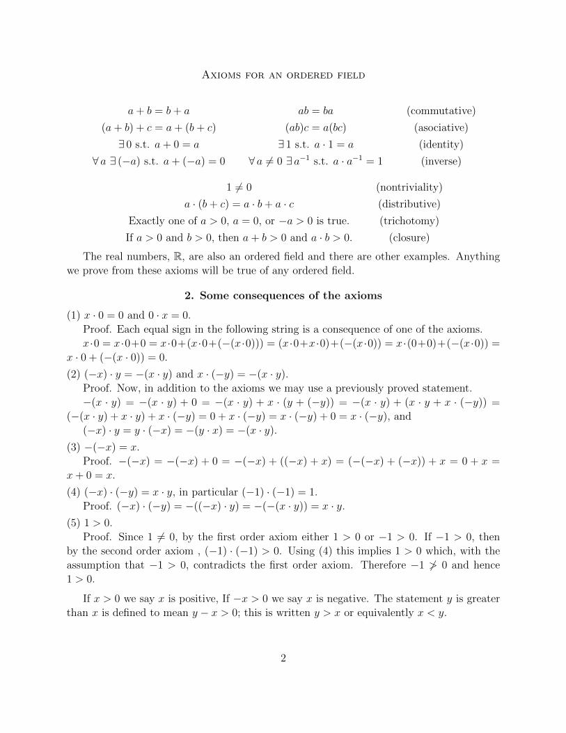
Axioms for an ordered field

a+ b = b+ a

(a+ b) + c = a+ (b+ c)

∃ 0 s.t. a+ 0 = a

∀ a ∃ (−a) s.t. a+ (−a) = 0

ab = ba

(ab)c = a(bc)

∃ 1 s.t. a · 1 = a

∀ a 6= 0 ∃ a−1 s.t. a · a−1 = 1

(commutative)

(asociative)

(identity)

(inverse)

1 6= 0

a · (b+ c) = a · b+ a · cExactly one of a > 0, a = 0, or −a > 0 is true.

If a > 0 and b > 0, then a+ b > 0 and a · b > 0.

(nontriviality)

(distributive)

(trichotomy)

(closure)

The real numbers, R, are also an ordered field and there are other examples. Anything

we prove from these axioms will be true of any ordered field.

2. Some consequences of the axioms

(1) x · 0 = 0 and 0 · x = 0.

Proof. Each equal sign in the following string is a consequence of one of the axioms.

x·0 = x·0+0 = x·0+(x·0+(−(x·0))) = (x·0+x·0)+(−(x·0)) = x·(0+0)+(−(x·0)) =

x · 0 + (−(x · 0)) = 0.

(2) (−x) · y = −(x · y) and x · (−y) = −(x · y).

Proof. Now, in addition to the axioms we may use a previously proved statement.

−(x · y) = −(x · y) + 0 = −(x · y) + x · (y + (−y)) = −(x · y) + (x · y + x · (−y)) =

(−(x · y) + x · y) + x · (−y) = 0 + x · (−y) = x · (−y) + 0 = x · (−y), and

(−x) · y = y · (−x) = −(y · x) = −(x · y).

(3) −(−x) = x.

Proof. −(−x) = −(−x) + 0 = −(−x) + ((−x) + x) = (−(−x) + (−x)) + x = 0 + x =

x+ 0 = x.

(4) (−x) · (−y) = x · y, in particular (−1) · (−1) = 1.

Proof. (−x) · (−y) = −((−x) · y) = −(−(x · y)) = x · y.

(5) 1 > 0.

Proof. Since 1 6= 0, by the first order axiom either 1 > 0 or −1 > 0. If −1 > 0, then

by the second order axiom , (−1) · (−1) > 0. Using (4) this implies 1 > 0 which, with the

assumption that −1 > 0, contradicts the first order axiom. Therefore −1 6> 0 and hence

1 > 0.

If x > 0 we say x is positive, If −x > 0 we say x is negative. The statement y is greater

than x is defined to mean y − x > 0; this is written y > x or equivalently x < y.

2

(6) Exactly one of x < y, x = y, or x > y is true.

Proof. These statements are equivalent to the statements y− x is positive, y− x = 0, or

−(y − x) is positive. Hence (6) is equivalent the first order axiom. The axiom and (6) are

called trichotomy.

(7) If x < y and z is in F , then x+ z < y + z.

Proof. We need to show that (y + z) − (x + z) is positive when y − x is positive. This

follows from a calculation, using the sum axioms, that (y + z)− (x+ z) = y − x.

(8) If x < y and y < z, then x < z.

Proof. By our hypothesis y − x and z − x are positive. Then by the second order axiom

the sum (z−y)+(y−x) positive. Using the sum axioms we calculate (z−y)+(y−x) = z−x.

Hence z − x is positive, so x < z.

(9) If x < y and 0 < z, then xz < yz.

Proof. By hypothesis, y−x is positive and z is positive, so the product (y−x)z is positive.

Using the distributive axiom and (2), we find (y+(−x))z = (yz)+((−x)z) = (yz)+(−(xz)).

It follows that xz < yz.

(10) If 0 < x and x < y, then x2 < y2.

Proof. By (9) x2 < xy. By (8) 0 < y, so by (9) xy < y2. Then by (8) x2 < y2.

(11) If 0 < x and 0 < y, then x2 < y2 ⇒ x < y.

Proof. We use the method of contradiction. We assume the hypotheses: 0 < x, 0 < y,

and x2 < y2. If x < y were false, then either x = y or y < x by (6) If we suppose x = y,

then x2 = y2. This contradicts the hypothesis. If we suppose y < x, then by (10), with the

roles of “x” and “y” interchanged, we have y2 < x2 which again contradicts the hypothesis.

Therefore x < y.

(12) If 0 < x and 0 < y, then x2 < y2 ⇐⇒ x < y.

Proof. This follows from (10) and (11).

(13) If xy = 0 then x = 0 or y = 0.

This will be an exercise. It can be proved for a field using the existence of multiplicative

inverses. It can also be proved for an ordered commutative ring (the integers or polynomials

over a field) in which multiplicative inverses may be missing.

3.√

2

Here is an algebraic version of Pythagoras’s geometric proof that the diagonal of a square

is not commensurable with its side.

Theorem. There is no rational number whose square is 2.

Proof. Otherwise there is a positive rational number whose square is 2. We could write√2 = m/n in such a way that n is the smallest possible denominator in N. Then 2n2 = m2.

We have m > n because m ≤ n implies m2 ≤ n2 < 2n2, a contradiction. Also m < 2n

because m ≥ 2n implies m2 ≥ 4n2 > 2n2, again a contradiction. Hence m− n < n. Finally,

(2n−m)2 = 4n2 − 4mn+m2 = 2m2 − 4mn+ 2n2 = 2(m− n)2.

3

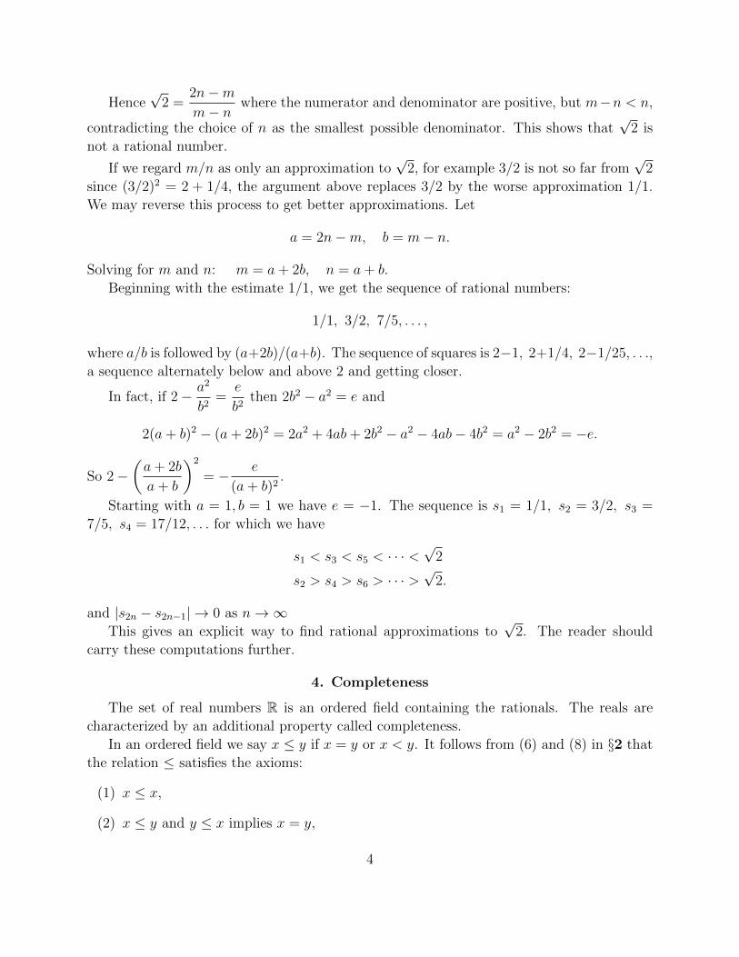
Hence√

2 =2n−mm− n

where the numerator and denominator are positive, but m−n < n,

contradicting the choice of n as the smallest possible denominator. This shows that√

2 is

not a rational number.

If we regard m/n as only an approximation to√

2, for example 3/2 is not so far from√

2

since (3/2)2 = 2 + 1/4, the argument above replaces 3/2 by the worse approximation 1/1.

We may reverse this process to get better approximations. Let

a = 2n−m, b = m− n.

Solving for m and n: m = a+ 2b, n = a+ b.

Beginning with the estimate 1/1, we get the sequence of rational numbers:

1/1, 3/2, 7/5, . . . ,

where a/b is followed by (a+2b)/(a+b). The sequence of squares is 2−1, 2+1/4, 2−1/25, . . .,

a sequence alternately below and above 2 and getting closer.

In fact, if 2− a2

b2=

e

b2then 2b2 − a2 = e and

2(a+ b)2 − (a+ 2b)2 = 2a2 + 4ab+ 2b2 − a2 − 4ab− 4b2 = a2 − 2b2 = −e.

So 2−(a+ 2b

a+ b

)2

= − e

(a+ b)2.

Starting with a = 1, b = 1 we have e = −1. The sequence is s1 = 1/1, s2 = 3/2, s3 =

7/5, s4 = 17/12, . . . for which we have

s1 < s3 < s5 < · · · <√

2

s2 > s4 > s6 > · · · >√

2.

and |s2n − s2n−1| → 0 as n→∞This gives an explicit way to find rational approximations to

√2. The reader should

carry these computations further.

4. Completeness

The set of real numbers R is an ordered field containing the rationals. The reals are

characterized by an additional property called completeness.

In an ordered field we say x ≤ y if x = y or x < y. It follows from (6) and (8) in §2 that

the relation ≤ satisfies the axioms:

(1) x ≤ x,

(2) x ≤ y and y ≤ x implies x = y,

4

(3) x ≤ y and y ≤ z implies x ≤ z, and

(4) for all x and y either x ≤ y or y ≤ x.

The first three axioms define a partial order and, with the fourth, a total order.

Completeness Axiom. If A and B are nonempty subsets of R and if x ∈ A and

y ∈ B ⇒ x ≤ y, then there exists a z ∈ R such that x ∈ A⇒ x ≤ z and y ∈ B ⇒ z ≤ y.

Definition. A nonempty closed bounded interval is a subset of R of the form

[a, b] = {x : a ≤ x ≤ b}

where a and b are real numbers with a ≤ b.

Definition. A sequence of such intervals, In = [an, bn], is nested if m < n ⇒ Im ⊃ In,

or equivalently if am ≤ an ≤ bn ≤ bm.

Cantor Intersection Theorem. If I1 ⊃ I2 ⊃ I3 ⊃ · · · is a sequence of nonempty

closed bounded intervals, then⋂∞

n=1 In is nonempty.

Proof. Let In = [an, bn] and let A = {an : n ∈ N}, B = {bn : n ∈ N}. Then

am ≤ am+n ≤ bm+n ≤ bn, hence A and B satisfy the hypothesis of the completeness axiom.

Hence there exists z ∈ R with an ≤ z ≤ bn, so for all n, z ∈ In. Therefore z ∈⋂∞

n=1 In.

Let λn = bn − an be the length of In. We say limn→∞

λn = 0 if

(∀ ε > 0)(∃ k)(n ≥ k ⇒ −ε < λn < ε).

Corollary. If limn→∞

λn = 0, then⋂∞

n=1 In contains a unique element.

Proof. If w and z are both in⋂∞

n=1 In with w < z, let ε = z − w > 0. Then (∃ k)(n ≥k ⇒ −ε < bn − an < ε). Also an ≤ w < z ≤ bn, so ε = z − w ≤ z − an ≤ bn − an < ε, a

contradiction.

Definition. An element b ∈ R is an upper bound for a nonempty set A if ∀x ∈ A, x ≤ b.

The nonempty subset A ⊂ R is bounded above if there exists an upper bound for A, that is

∃ b ∈ R such that x ∈ A⇒ x ≤ b.

Definition. We say z ∈ R is a least upper bound for A if

(1) z is an upper bound for A and

(2) if b is any upper bound for A, then z ≤ b.

Lemma. If A has a least upper bound, it is unique.

Proof. If z and z1 are both least upper bounds for A, then z ≤ z1 since z1 is an upper

bound and z is a least upper bound. Also z1 ≤ z since z is an upper bound and z1 is a least

upper bound. Therefore z = z1.

5

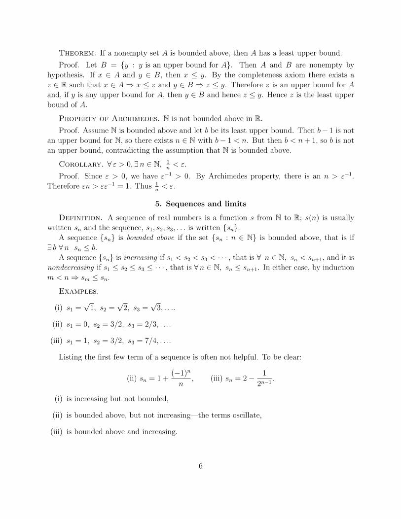
Theorem. If a nonempty set A is bounded above, then A has a least upper bound.

Proof. Let B = {y : y is an upper bound for A}. Then A and B are nonempty by

hypothesis. If x ∈ A and y ∈ B, then x ≤ y. By the completeness axiom there exists a

z ∈ R such that x ∈ A ⇒ x ≤ z and y ∈ B ⇒ z ≤ y. Therefore z is an upper bound for A

and, if y is any upper bound for A, then y ∈ B and hence z ≤ y. Hence z is the least upper

bound of A.

Property of Archimedes. N is not bounded above in R.

Proof. Assume N is bounded above and let b be its least upper bound. Then b− 1 is not

an upper bound for N, so there exists n ∈ N with b− 1 < n. But then b < n+ 1, so b is not

an upper bound, contradicting the assumption that N is bounded above.

Corollary. ∀ ε > 0,∃n ∈ N, 1n< ε.

Proof. Since ε > 0, we have ε−1 > 0. By Archimedes property, there is an n > ε−1.

Therefore εn > εε−1 = 1. Thus 1n< ε.

5. Sequences and limits

Definition. A sequence of real numbers is a function s from N to R; s(n) is usually

written sn and the sequence, s1, s2, s3, . . . is written {sn}.A sequence {sn} is bounded above if the set {sn : n ∈ N} is bounded above, that is if

∃ b ∀n sn ≤ b.

A sequence {sn} is increasing if s1 < s2 < s3 < · · · , that is ∀ n ∈ N, sn < sn+1, and it is

nondecreasing if s1 ≤ s2 ≤ s3 ≤ · · · , that is ∀n ∈ N, sn ≤ sn+1. In either case, by induction

m < n⇒ sm ≤ sn.

Examples.

(i) s1 =√

1, s2 =√

2, s3 =√

3, . . ..

(ii) s1 = 0, s2 = 3/2, s3 = 2/3, . . ..

(iii) s1 = 1, s2 = 3/2, s3 = 7/4, . . ..

Listing the first few term of a sequence is often not helpful. To be clear:

(ii) sn = 1 +(−1)n

n, (iii) sn = 2− 1

2n−1 .

(i) is increasing but not bounded,

(ii) is bounded above, but not increasing—the terms oscillate,

(iii) is bounded above and increasing.

6

Definition. The sequence {sn} converges to ` if

(∀ ε > 0)(∃m ∈ N)(n > m⇒ −ε < sn − ` < ε).

The sequence converges if there is an ` ∈ R such that {sn} converges to `, that is,

(∃ ` ∈ R)(∀ ε > 0)(∃m ∈ N)(n > m⇒ −ε < sn − ` < ε).

We write limn→∞

sn = ` to mean that the sequence {sn} converges to `. We say limn→∞

sn

exists if the sequence converges.

Example. Using this definition we show that the sequence {1/n} converges to 0.

Given ε > 0, by the Corollary to Archimedes property, we know there is an integer m

with 1/m < ε. If n ≥ m, then 0 < 1/n ≤ 1/m < ε, hence −ε < 1/n − 0 < ε. Hence the

definition is satisfied.

Uniqueness of limits. If lim sn = ` and lim sn = k, then k = `.

Proof. Otherwise we may assume k < `, relabeling if necessary. Let ε = (` − k)/2 > 0.

There is an m such that

n > m⇒ −ε < sn − `, hence ε = −ε+ `− k < sn − `+ `− k = sn − k.

Therefore lim sn = k is false contradicting the assumption k < `.

The following result gives convergence without specifying the limit.

Theorem. If a sequence is nondecreasing and bounded above, then the sequence con-

verges.

Proof. Let A = {sn : n ∈ N}. By hypothesis A is bounded above. Hence A has a least

upper bound, call it `. Then (∀n)(sn ≤ `). If ε > 0, then ` − ε is not an upper bound, so

(∃m)(`− ε < sm). Since the sequence is nondecreasing, if n ≥ m then sm ≤ sn. Therefore,

n ≥ m⇒ `− ε < sm ≤ sn ≤ ` < `+ ε.

Hence n ≥ m⇒ −ε < sn − ` < ε.

Example. Consider the sequence

√3,

√3 +√

3,

√3 +

√3 +√

3, . . .

defined recursively by s1 =√

3 and sn+1 =√

3 + sn.

This sequence is bounded above: s1 =√

3 < 3 and, if sn < 3 then 3 + sn < 6 < 9, so

sn+1 < 3.

The sequence is increasing. 3 < 3 +√

3, so s1 < s2. If sn < sn+1, then 3 + sn < 3 + sn+1,

so sn+2 < sn+1. Hence the sequence converges. At this point we do not know the limit.

Knowing that it exists will lead to a proof that the limit is (1 +√

13)/2.

7

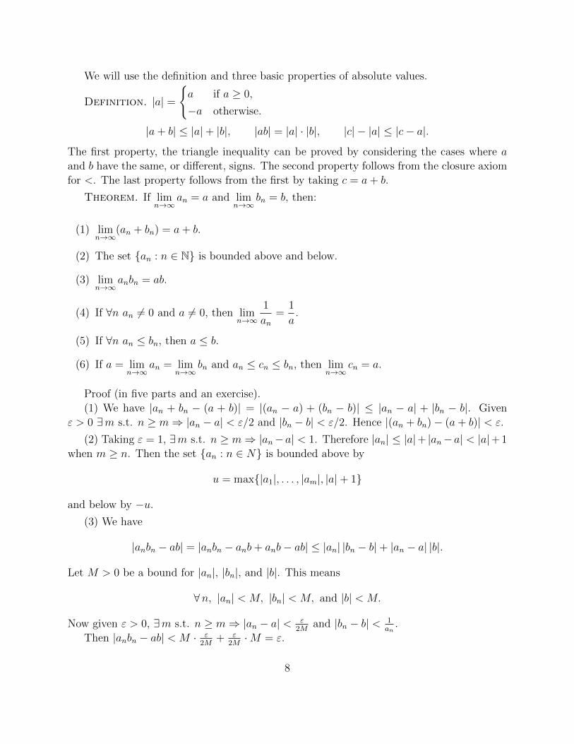
We will use the definition and three basic properties of absolute values.

Definition. |a| =

{a if a ≥ 0,

−a otherwise.

|a+ b| ≤ |a|+ |b|, |ab| = |a| · |b|, |c| − |a| ≤ |c− a|.

The first property, the triangle inequality can be proved by considering the cases where a

and b have the same, or different, signs. The second property follows from the closure axiom

for <. The last property follows from the first by taking c = a+ b.

Theorem. If limn→∞

an = a and limn→∞

bn = b, then:

(1) limn→∞

(an + bn) = a+ b.

(2) The set {an : n ∈ N} is bounded above and below.

(3) limn→∞

anbn = ab.

(4) If ∀n an 6= 0 and a 6= 0, then limn→∞

1

an=

1

a.

(5) If ∀n an ≤ bn, then a ≤ b.

(6) If a = limn→∞

an = limn→∞

bn and an ≤ cn ≤ bn, then limn→∞

cn = a.

Proof (in five parts and an exercise).

(1) We have |an + bn − (a + b)| = |(an − a) + (bn − b)| ≤ |an − a| + |bn − b|. Given

ε > 0 ∃m s.t. n ≥ m⇒ |an − a| < ε/2 and |bn − b| < ε/2. Hence |(an + bn)− (a+ b)| < ε.

(2) Taking ε = 1, ∃m s.t. n ≥ m⇒ |an−a| < 1. Therefore |an| ≤ |a|+ |an−a| < |a|+ 1

when m ≥ n. Then the set {an : n ∈ N} is bounded above by

u = max{|a1|, . . . , |am|, |a|+ 1}

and below by −u.

(3) We have

|anbn − ab| = |anbn − anb+ anb− ab| ≤ |an| |bn − b|+ |an − a| |b|.

Let M > 0 be a bound for |an|, |bn|, and |b|. This means

∀n, |an| < M, |bn| < M, and |b| < M.

Now given ε > 0, ∃m s.t. n ≥ m⇒ |an − a| < ε2M

and |bn − b| < 1an

.

Then |anbn − ab| < M · ε2M

+ ε2M·M = ε.

8

(4) We first prove that {1/an} is bounded. Let ε = |a|/2 > 0. Then ∃m s.t. n ≥ m ⇒|an− a| < |a|/2. Hence |a| − |an| < |a|/2, so that |a|/2 < |an| or, equivalently, 1/|an| < 2/|a|for n ≥ m. Let

M = max

{1

|a1|, . . . ,

1

|am|,

2

|a|

}.

Then 1/|an| < M for all n. Next∣∣∣∣ 1

an− 1

a

∣∣∣∣ =

∣∣∣∣an − aaan

∣∣∣∣ =1

|a||an − a|

1

|an|≤ 1

|a||an − a|M.

Now, given ε > 0,

∃m s.t. n ≥ m⇒ |an − a| <ε|a|M

.

Hence |1/an − 1/a| < ε.

(5) This proof is by contradiction. Assume a > b and let ε = (a− b)/2 > 0. Then

∃m s.t. n ≥ m⇒ |an − a| < ε/2 and |bn − b| < ε/2.

Then |b− a+ an − bn| = |an − a+ b− bn| < (a− b)/2.

Since b − a < 0 by assumption and an − bn ≤ 0 by hypothesis, b − a + an − bn < 0

and its absolute value is a − b − an + bn < (a − b)/2 by the line above. This implies

(a− b)/2 < an − bn ≤ 0, a contradiction, therefore a ≤ b.

(6) This result, known as the pinching theorem, is left as an exercise.

6. Series

The finite geometric series is the sum

sn = 1 + x+ x2 + · · ·+ xn−1.

Lemma 1. (x− 1)sn = xn − 1.

Proof. s1 = 1, so the statement is true when n = 1. If we assume the statement is true for

n, then (x−1)sn+1 = (x−1)(sn+xn) = (x−1)sn+(x−1)xn = xn−1+xn+1−xn = xn+1−1.

So by induction the statement is true for all n.

Lemma 2. If x ≥ 1, then sn ≥ n and xn ≥ 1 + (x− 1)n.

Proof. If x ≥ 1, then each xj ≥ 1, so from the definition sn ≥ n. The second statement

follows from Lemma 1.

Lemma 3. If x > 1, then the sequence {xn} is not bounded above.

Proof. If x > 1, then ∀ b ∃m s.t. m > b/(x− 1). Then n ≥ m⇒ xn > b.

Lemma 4. If |x| < 1, then limn→∞

xn = 0.

Proof. If x = 0, then each xn = 0. Assume 0 < |x| < 1. Then 1/|x| > 1. Given ε > 0,

by Lemma 3, ∃m s.t. n ≥ m⇒ |1/x|n > 1/ε, hence |xn| < ε.

9

Theorem. If |x| < 1 then limn→∞

sn =1

1− x.

Proof.

limn→∞

sn = limn→∞

1− xn

1− x=

1

1− x

(1− lim

n→∞xn)

=1

1− x.

This result is also written∞∑n=0

xn =1

1− x; sn =

n−1∑i=0

xi is called a partial sum of the

infinite series∞∑n=0

xn. In general, given a sequence {an}, sm =m∑

n=1

an is called the mth

partial sum of the series∞∑n=1

an.

Definition. If the sequence {sm} converges to `, we say the infinite series∞∑n=1

an con-

verges to `.

Theorem. If∞∑n=1

an = a and∞∑n=1

bn = b, then∞∑n=1

(an + bn) = a+ b and∞∑n=1

can = ca.

Proof. The first part follows from part 1 of the Theorem of §4 applied to the sequence of

partial sums {sm} and {tm}. For the second part let {tm} be the constant sequence, tm = c

and use part 3 of the Theorem.

Two widely known geometric series are the decimal expansion 0.9999 · · · which is

9

10+

9

102+

9

103· · · = 9

10×∞∑n=0

1

10

n

=9

10× 1

1− 1/10= 1

and the sum1

2+

1

4+

1

8+ · · · = 1.

7. Series of nonnegative terms

If an ≥ 0 we say∞∑n=0

an is a series of nonnegative terms. In this case the sequence of

partial sums {sm} is nondecreasing. If {sm} is bounded above, then the series converges by

§5.

For example consider the series∞∑n=1

1

n(n+ 1). Computing the first several partial sums

suggests sm = 1 − 1/(m + 1) which can be proved by induction. Hence {sm} is increasing

and bounded above by 1. Thus the series converges. In fact we know that lim sm = 1, so

the series converges to 1.

10

Now consider the series∞∑n=1

1

n2. Explicit partials sums are not revealing. Comparing

partials sums with the previous series, we have

1 +1

2 · 2+

1

3 · 3+ · · ·+ 1

m ·m< 1 +

1

1 · 2+

1

2 · 3+ · · ·+ 1

(m− 1) ·m= 1 + 1− 1

m< 2.

Again this implies this sum converges to a limit between 1 and 2. The limit can be shown

to be π2/6.

For the series∞∑n=0

1

n!= 1 + 1 +

1

2+

1

2 · 3+ · · · , the nth term,

1

n!<

1

(n− 1)n. Comparing

terms we have

1 + 1 +1

2!+ · · ·+ 1

n!≤ 1 + 1 +

1

1 · 2+ · · ·+ 1

(n− 1)n< 3.

Hence this series converges to a number, e, between 2 and 3.

To prove from the definition that a series converges we need to know the limit ` of

the partial sums. Often the limit is not known but, if it exists, is some new object of

mathematical interest about which we would like to know more. In that case we need some

theoretical argument to show convergence. The result used above, called the comparison

theorem, can be stated as follows:

Theorem. If an ≥ 0 and if ∃ b s.t. ∀m,m∑

n=1

an < b, then∞∑n=1

an converges.

8. Limits of functions and continuity

Definition. limx→a

f(x) = ` means

(∀ ε > 0)(∃ δ > 0)(0 < |x− a| < δ ⇒ |f(x)− `| < ε).

The set {x : f is defined at x} is called the domain of f , written dom f . If x /∈ dom f

then |f(x) − `| < ε is false. Hence for limx→a

f(x) to exist, there must be some δ > 0 with

{x : 0 < |x− a| < δ} ⊂ dom f . The value of f at a, or even whether f is defined at a, does

not matter.

Uniqueness of limits. If limx→a

f(x) = ` and limx→a

f(x) = k, then k = `.

Proof. If k 6= `, then let 2ε = |`− k| > 0. Then

(∃ δ > 0)(0 < |x− a| < δ ⇒ |f(x)− 0`| < ε, |f(x)− k| < ε), hence

2ε = |`− k| = |`− f(x) + f(x)− k| ≤ |`− f(x)|+ |f(x)− k| < 2ε,

a contradiction.. Hence k = `.

11

Theorem. Let limx→a

f(x) = ` and limx→a

g(x) = m. Then:

(1) limx→a

(f(x) + g(x)) = `+m.

Proof. Given ε > 0, (∃ δ1 > 0)(0 < |x− a| < δ1 ⇒ |f(x)− `| < ε/2) and

(∃ δ2 > 0)(0 < |x− a| < δ2 ⇒ |g(x)−m| < ε/2).

Take δ = min{δ1, δ2}. Then 0 < |x− a| < δ implies

|f(x) + g(x)− `−m| ≤ |f(x)− `|+ |g(x)−m| < ε.

(2) (∃ δ > 0)(0 < |x− a| < δ ⇒ |f(x)| < |`|+ 1).

Proof. Let ε = 1 then (∃ δ > 0)(0 < |x − a| < δ ⇒ |f(x) − `| < 1). Hence

|f(x)| = |`+ f(s)− `| ≤ |`|+ |f(x)− `| < |`|+ 1.

(3) limx→a

(f(x)g(x)) = `m.

Proof. Taking the minimum of three values for δ we find δ > 0 such that 0 < |x−a| < δ

implies |f(x)| < |`|+1, and |g(x)−m| < ε/(2(|`|+1)), and |f(x)−`| < ε/(2(|m|+1)).

Then

|f(x)g(x)− `m| = |f(x)g(x)− f(x)m+ f(x)m− `m|≤ |f(x)| |g(x)−m|+ |f(x)− `| |m|

< (|`|+ 1)ε

2(|`|+ 1)+

ε

2(|m|+ 1)|m|

< ε.

(4) If ` 6= 0, (∃ δ > 0)(0 < |x− a| < δ ⇒ |f(x)| > |`|/2).

Proof. Since |`|/2 > 0, (∃ δ > 0)(0 < |x − a| < δ ⇒ |f(x) − `| < |`|/2). Then

|`| − |f(x)| ≤ |`− f(x)| < |`|/2, so |`|/2 < |f(x)|.

(5) If ` 6= 0, then limx→a

1

f(x)=

1

`.

Proof. Given ε > 0, take δ > 0 so that 0 < |x − a| < δ implies |f(x)| > |`|/2 and

|f(x)− `| < ε`2/2. Then

∣∣∣∣ 1

f(x)− 1

`

∣∣∣∣ =|f(x)− `||`| |f(x)|

< ε.

Definition. f is continuous at a if limx→a

f(x) = f(a)

Hence f is continuous at a if (∀ ε > 0)(∃ δ > o)(|x− a| < δ ⇒ |f(x)− f(a)| < ε).

12

Proposition. A constant function, f(x) = c, and the identity function, f(x) = x, are

continuous at every a ∈ R.

Proof. For f(x) = c, given ε > 0, for any a and any x, |f(x) − f(a)| = |c − c| = 0 < ε.

For f(x) = x we may take δ = ε since then, if |x− a| < δ we have |x− a| < ε.

Corollary. Any polynomial function is continuous at all a ∈ R. Any ratio of polyno-

mials is continuous at any a which is not a root of the denominator.

Proposition. If limn→∞

sn = ` and f is continuous at `, then limn→∞

f(sn) = f(`).

Proof. Given ε > 0, (∃ δ > 0)(|x − a| < δ ⇒ |f(x) − f(`)| < ε) and (∃ k)(n ≥ k ⇒|sn − `| < δ). Hence n ≥ k implies |f(sn)− f(`)| < ε. Therefore lim

n→∞f(sn) = f(`).

Proposition. If f(a) = b, f is continuous at a, and g is continuous at b, then g ◦ f is

continuous at a.

Proof. Since g is continuous at b, given ε > 0, ∃ δ > 0 such that |y − b| < δ ⇒|g(y) − g(b)| < ε. Then since f is continuous at a and δ > 0, ∃ γ > 0 such that |x − a| <γ ⇒ |f(x)− f(a)| < δ.

Hence |g(f(x))− g(f(a))| < ε provided |x−a| < γ and therefore g ◦ f is continuous at a.

9. Functions continuous on an interval

Intermediate Value Theorem. If f is continuous on [a, b] and f(a)f(b) < 0, then

there exists z ∈ [a, b] such that f(z) = 0.

Proof. Assume that f(a) < 0 and f(b) > 0. (In the opposite case, replace f by −f .)

Let I0 = [a, b]. We construct recursively a nested sequence of nonempty, bounded, closed

intervals. If In = [an, bn] has been constructed with f(an) < 0 and f(bn) > 0, let x =

(bn − an)/2 be its midpoint. Define In+1 by

an+1 = an, bn+1 = x if f(x) > 0,

an+1 = x, bn+1 = bn if f(x) < 0.

(In the case f(x) = 0, we may take z = x and the proof is complete.) By the Cantor

intersection theorem there exists z ∈⋂∞

n=1 In.

We claim that f(z) = 0. If f(z) > 0, then there is a δ > 0 such that

0 < |x− z| < δ ⇒ −f(z) < f(x)− f(z) < f(z), and therefore f(x) > 0.

Further there exists n such that bn−an = (b−a)/2n < δ. Now an ≤ z ≤ bn, so 0 ≤ z−an ≤bn − an ≤ δ, so f(an) > 0 which contradicts the construction of an.

Similarly, f(z) < 0 leads to a contradiction. Therefore f(z) = 0.

Example. Given c > 0, let f(x) = x2 − c and take b = max{c, 2}. Then f(0) = −c < 0

and, in either case, f(b) > 2 > 0. By the intermediate value theorem, there exists z > 0

with z2 = c.

Definition. A function f is bounded above on [a, b] is there exists k such that a ≤ x ≤b ⇒ f(x) ≤ k.

13

Boundedness Theorem. If f is continuous on [a, b], then f is bounded above on [a, b].

Lemma. Suppose a < c < b. If f is bounded above on [a, c] and on [c, b], then f is

bounded above on [a, b].

Proof. By hypothesis, (∃ k1)(a ≤ x ≤ c ⇒ f(x) ≤ k1) and (∃ k2)(c ≤ x ≤ b ⇒ f(x) ≤k2). Then if a ≤ x ≤ b, either x ≤ c and f(x) ≤ k1 or c ≤ x and f(x) ≤ k2. Therefore

f(x) ≤ max{k1, k2}.Proof of theorem. Say f is not bounded on I0 = [a, b]. We construct recursively a nested

sequence of nonempty, bounded, closed intervals on which f is unbounded. If In = [an, bn]

has been constructed and f is unbounded on In, let x = (bn − an)/2 be its midpoint. By

the lemma, f is unbounded on at least one of the intervals [a, x] or [x, b]. Let In+1 be one of

these on which f is unbounded.

By the Cantor intersection theorem there exists z ∈⋂∞

n=1 In. Since f is continuous at z,

there exists δ > 0 such that |x − z| < δ ⇒ f(x) ≤ f(z) + 1. But there exists n such that

bn − an = (b − a)/2n < δ and an ≤ z ≤ bn. If an ≤ x ≤ bn, then |x − z| ≤ bn − an < δ so

f(x) ≤ f(z) + 1. Hence f is bounded above on In, contradicting the construction. Therefore

f is bounded above on [a, b].

Extreme Value Theorem. If f is continuous on [a, b], then there exist numbers

m,M, c1, c2 such that

m ≤ f(x) ≤M for x ∈ [a, b],

f(c1) = m, f(c2) = M, where c1, c2 ∈ [a, b].

Proof. We prove this for M and c2 and apply this result to −f to get m and c1. By the

previous theorem the set {f(x) : x ∈ [a, b]} is bounded. Hence there is a least upper bound

M . Suppose for all x ∈ [a, b], f(x) 6= M . Then f(x) < M and hence the function

g(x) =1

M − f(x)for x ∈ [a, b]

is continuous. Again by the previous theorem, there is a bound k such that

0 <1

M − f(x)≤ k and hence M − f(x) ≥ 1

kor f(x) ≤M − 1

k< M.

This contradicts the fact that M is the least upper bound. Therefore there is a c2 with

f(c2) = M .

10. Inverse functions

Let A and B be subsets of R and let f be a function with domain A which takes values

in B, f(x) ∈ B. We write f : A −→ B and call f a function, or a map, from A to B.

Definitions. The image of f , im f = f(A) = {y : ∃x ∈ A, f(x) = y};

14

f is surjective or onto B if im f = B;

f is injective or one-to-one if f(u) = f(x) ⇒ u = x;

The identity map 1A : a −→ A is defined by 1A(x) = x for all x ∈ A;

A map g : B −→ A is an inverse of f if g ◦ f = 1A and f ◦ g = 1B.

Notice that f(x) = y if and only if g(y) = x. If f : A −→ B has an inverse, the inverse

is unique, and if g : B −→ A is an inverse of f , then f is an inverse of g.

Proposition. If (g ◦ f) = 1A, then f is one-to-one and g is onto.

Proof. If f(u) = f(x), then u = (g ◦ f)(u) = g(f(u)) = g(f(x)) = (g ◦ f)(x) = x, so f is

one-to-one. If x ∈ A, let y = f(x). Then g(y) = g(f(x)) = x, so g is onto.

Proposition. f : A −→ B has an inverse if and only if f is one-to-one and onto.

Proof. If f has an inverse, g, then (g ◦ f) = 1A, so f is one-to-one. Also f ◦ g = 1B, so

f is onto by the previous proposition. Conversely, given y ∈ B, if f is onto, ∃x ∈ A with

f(x) = y. Since f is one-to-one, this x is unique. Thus g is well-defined if we set g(y) = x.

Our goal is to prove that if f is continuous and has a inverse, then the inverse is contin-

uous.

A more general type of interval than the nonempty, closed, bounded intervals used so far

is given by the following

Definition. An interval is a set I such that, if a, b ∈ I and a ≤ x ≤ b, then x ∈ I.

Theorem. If f is defined and continuous on an interval I and f is one-to-one, then f is

either increasing or f is decreasing on I.

Proof. The proof is an application of the intermediate value theorem. Let a, b, c, d ∈ I,

a < b, c < d, and suppose that f(a) < f(b). (If not, replace f by −f .) We must prove that

f(c) < f(d). We define a family of intervals [xt, yt] for 0 ≤ t ≤ 1 with x0 = a, y0 = b and

x1 = c, y1 = d.

Set xt = (1−t)a+tc and yt = (1−t)b+td. Note that yt−xt = (1−t)(b−a)+t(d−c) > 0

for 0 ≤ t ≤ 1, so xt < yt.

Define h : [0, 1] −→ R by h(t) = f(xt)− f(yt); h is a continuous function of t since it is

a composition of continuous functions.

Since f is one-to-one, h(t) 6= 0. Now h(0) = f(a)− f(b) < 0. Then, by the intermediate

value theorem applied to h on the interval [0, 1], we must have f(c) < f(d), hence f is

increasing.

Lemma. If f is continuous on an interval I, then J = f(I) is an interval.

Proof. Given u, v ∈ J, ∃ a, b ∈ I such that f(u) = a, f(b) = v. Since I is an interval,

[a, b] ⊂ I so f is defined on [a, b]. If y ∈ [u, v], then f(a) ≤ y ≤ f(b), so by the intermediate

value theorem ∃x ∈ [a, b] with f(x) = y. Therefore y ∈ J and hence J is an interval.

Lemma. If f : I −→ J and g : J −→ I are inverse functions and f is increasing, then g

is also increasing.

Proof. Given u, v ∈ J with u < v, let g(u) = a, g(v) = b. If a ≥ b then u = f(a) ≥f(b) = v, a contradiction, hence a < b and g is increasing.

15

Theorem. If f : I −→ J and g : J −→ I are inverse functions and f is continuous, then

g is also continuous.

Proof. Assume that f is increasing (and apply this result to −f if f is decreasing). Given

y ∈ J we must show the limv→y

g(v) = g(y). Given ε > 0 we need δ > 0 such that

|v − y| < δ ⇒ |g(v)− g(y)| < ε,

or equivalently

y − δ < v < y + δ ⇒ g(y)− ε < g(v) < g(y) + ε.

Let y = f(x) and v = f(u). Since x− ε < x < x+ ε and f is increasing we have

f(x− ε) < f(x) < f(x+ ε).

Let δ = min{f(x+ ε)− f(x), f(x)− f(x− ε)}. If y − δ < v < y + δ, then

f(x− ε) = y −(f(x)− f(x− ε)

)≤ y − δ < v < y + δ ≤ y +

(f(x+ ε)− f(x)

)= f(x+ ε).

Since g is increasing and x = g(y) we have

g(y)− ε < g(v) < g(y) + ε.

Examples. The power functions fn(x) = xn, n > 0, are increasing on R if n is odd and

on [0,∞) if n is even. The inverse functions are n√x. The compositions xm/n are continuous.

For nonrational exponents a further limit argument, or the definition xa = exp(a lnx) for

x > 0 is needed.

Let f(x) =√

3 + x. The sequence defined in §5 by s1 =√

3 and sn+1 = f(sn) was

shown there to converge to a real number ` ∈ [1, 3]. Since f is continuous on [0,∞),

f(`) = f(lim sn) = lim f(sn) = lim sn+1 = `. By the quadratic formula, ` = (1 +√

13)/2.

11. Differentiation

Definition. The derivative of f at a is

f ′(a) = limx→a

f(x)− f(a)

x− a.

If this limit exists, f is said to be differentiable at a.

Examples. If f(x) = c for some real number c, then f ′(a) = 0 for any a.

Recall the finite geometric series from §6. In

(x− 1)(1 + x+ x2 + · · ·+ xn−1) = xn − 1,

replace x with x/a and multiply by an to get

(x− a)(an−1 + an−2x+ · · ·+ xn−1) = xn − an. (∗)

16

Set

ϕa(x) =n−1∑i=0

an−1−ixi.

Then ϕa is continuous at a (and for all x). If x 6= a, then ϕa(x) = (xn − an)/(x− a). Hence

limx→a

xn − an

x− a= lim

x→aϕa(x) = nan−1. Thus if f(x) = xn, f ′(a) = nan−1.

Next divide equation (∗) by anxn for a, x 6= 0 to get

(x− a)(a−1x−n + a−2x−n+1 + · · ·+ a−nx−1) = a−n − x−n.

Thus for a, x 6= 0,

(x−n − a−n)/(x− a) = −(ax)−1ϕa−1(x−1) = ψa(x)

and ψa is continuous at x = a 6= 0. Thus if f(x) = x−n, f ′(a) = −na−n−1.Finally, replace x by x1/n and a by a1/n in equation (∗) to find

x1/n − a1/n

x− a=

1

ϕa1/n(x1/n)

and deduce that the derivative of f(x) = x1/n = n√x is f ′(a) = 1

na

1n−1.

In the three cases above we introduced functions which were equal to the difference

quotient for x 6= a and which were continuous at a. Constantin Caratheodory gave an

equivalent reformulation of the definition of the derivative in terms of such a function. His

definition leads to shorter proofs and makes the use of continuity more explicit.

Caratheodory’s Theorem. f is differentiable at a if and only if there is a function

ϕa(x) which is continuous at a such that

f(x) = f(a) + (x− a)ϕa(x).

If f is differentiable, then f ′(a) = ϕa(a).

Proof. Assume such a function ϕa(x) exists. Then (f(x) − f(a))/(x − a) = ϕa(x) for

x 6= a and limx→a

(f(x)− f(a))/(x− a) = limx→a

ϕa(x) = ϕa(a).

Conversely, assume f is differentiable at a and f ′(a) = ` Define

ϕa(x) =

{(f(x)− f(a))/(x− a) if x 6= a,

` if x = a.

Then limx→a

ϕa(x) = limx→a

(f(x)− f(a))/(x− a) = `, so ϕa(x) is continuous at a.

Caratheodory’s definition is the subject of an article by Stephen Huhn in the American

Mathematical Monthly 98 (Jan. 1991) pp. 40–44.

17

Theorem. If f is differentiable at a then f is continuous at a.

Proof. By Caratheodory, f(x) = f(a) + (x − a)ϕa(x) where ϕa(x) is continuous at a.

Then by the results of §8, f is continuous at a.

Sum rule. If f and g are differentiable at a, then f + g is differentiable at a and

(f + g)′(a) = f ′(a) + g′(a).

Proof. We have f(x) = f(a) + (x − a)ϕa(x) and g(x) = g(a) + (x − a)ψa(x), hence

(f + g)(x) = (f + g)(a) + (x − a)(ϕa(x) + ψa(x)). By §8, ϕa + ψa is continuous at a and

(ϕa + ψa)(a) = ϕa(a) + ψa(a).

Product rule. If f and g are differentiable at a, then fg is differentiable at a and

(fg)′(a) = f ′(a)g(a) + f(a)g′(a).

Proof. As above,

(fg)(x) =(f(a) + (x− a)ϕa(x)

)(g(a) + (x− a)ψa(x)

)= (fg)(a) + (x− a)

(ϕa(x)g(a) + f(a)ψa(x) + (x− a)ϕa(x)ψa(x)

)where ϕa(x)g(a) + f(a)ψa(x) + (x − a)ϕa(x)ψa(x) is continuous at a and at x = a is equal

to f ′(a)g(a) + f(a)g′(a).

Corollary (Linearity). (kf + `g)′ = kf ′ + `g′ for k, ` ∈ R.

Chain rule. If f is differentiable at a, f(a) = b, and g is differentiable at b, then the

composition g ◦ f is differentiable at a and (g ◦ f)′(a) = g′(b)f ′(a).

Proof.

(g ◦ f)(x) = g(f(x)) = g(b) + (f(x)− b)ψb(f(x))

= g(b) +(f(a) + (x− a)ϕa(x)− b

)ψb(f(x))

= g(b) + (x− a)ϕa(x)ψb(f(x)).

Since f is continuous at a, ψb ◦ f is continuous at a so (ψb ◦ f)ϕa is continuous at a and

ψb(f(a))ϕa(a) = g′(b)f ′(a).

Proposition. Let f be differentiable at a and f(a) 6= 0. Then

(1/f)′(a) = −f ′(a)/(f(a))2.

Proof. If g(y) = y−1, g is differentiable at b = f(a) and g′(b) = −b−2. Then (g ◦ f)(x) =

1/f(x) and (g ◦ f)′(a) = −(f(a))−2f ′(a).

Quotient rule. Let f and g be differentiable at a with g(a) 6= 0. Then(f

g

)′(a) =

f ′(a)g(a)− f(a)g′(a)

g(a)2.

18

Proof. Write

(f

g

)(x) as the product f(x) · (1/g(x)) and use the previous proposition

and the product rule.

Inverse Function Theorem. If f : I −→ J and g : J −→ I are inverses and f

is differentiable at a ∈ I with f ′(a) 6= 0, then g is differentiable at b = f(a) and g′(b) =

1/f ′(g(b)).

Proof. We have f(x) = f(a)+(x−a)ϕa(x) where ϕa is continuous at a and f ′(a) = ϕa(a).

Since g is continuous at b and ϕa is continuous at g(b), ϕa ◦ g is continuous at b and

ϕa(g(b)) = f ′(a) 6= 0. Hence there exists ε > 0 such that when |y − b| < ε, ϕa(g(y)) 6= 0.

Let y = f(x) and x = g(y). Then

y = b+ (g(y)− g(b))ϕa(x), hence g(y) = g(b) + (y − b)/ϕa(g(y)).

Therefore g′(b) = 1/f ′(g(b)).

Theorem. If f ′(a) > 0, then there is a δ > 0 such that

a− δ < x < a ⇒ f(a) < f(x)

a < x < a+ δ ⇒ f(x) < f(a).

Proof. Again f(x) = f(a)+(x−a)ϕa(x), ϕa is continuous at a, and ϕa(a) > 0. Therefore

there is a δ > 0 such that |x − a| < δ ⇒ ϕa(x) > 0. If a < x < a + δ then x − a > 0

and f(a) < f(a) + (x − a)ϕa(x) = f(x), while if a − δ < x < a then x − a < 0 and

f(a) > f(a) + (x− a)ϕa(x) = f(x).

Definition. A critical point for f is a number c such that f ′(c) = 0.

The critical point test for extreme values is the following:

Corollary. Let f be defined on (a, b), a < c < b, and f be differentiable at c. If

f(x) ≤ f(c) for all x ∈ (a, b) or if f(x) ≥ f(c) for all x ∈ (a, b), then f ′(c) = 0.

Thus if f is defined on [a, b] and c ∈ [a, b] is an extreme point of f , then c is either an

end point of [a, b], a point where f is not differentiable, or a critical point of f .

Proof. By contradiction, applying the theorem to either f or −f .

The conclusion of the previous theorem is sometimes described by saying that f is in-

creasing at a. This does not imply that f is increasing on any interval. An example of a

function which is increasing at 0, but not in any interval (0, δ) or (−δ, 0) for any δ > 0 is

f(x) =

{0, if x = 0;

x/2 + x2 sin(1/x), otherwise.

This function is differentiable at 0 and in fact on R, but f ′ is not continuous at 0.

19

12. Functions differentiable on an interval

Rolle’s Theorem. If f is continuous on [a, b] and differentiable on (a, b), and if f(a) =

f(b), then ∃ ξ ∈ (a, b) such that f ′(ξ) = 0.

Proof. Since f is continuous on [a, b], f has an extreme value on [a, b] by (§9). If a

maximum point or a minimum point occurs at ξ ∈ (a, b), then by the critical point test,

f ′(ξ) = 0. If both the maximum and minimum values occur at the end points then, since

f(a) = f(b), f is constant on [a, b] and f ′(ξ) = 0 for any ξ ∈ (a, b).

Mean Value Theorem. If f is continuous on [a, b] and differentiable on (a, b), then

∃ ξ ∈ (a, b) such that (f(b)− f(a))/(b− a) = f ′(ξ).

Proof. Let h(x) = f(x) − f(b)− f(a)

b− a(x − a). Then h(a) = f(a) and h(b) = f(a), so h

satisfies the hypotheses of Rolle’s theorem. Therefore ∃ ξ ∈ (a, b) such that h′(ξ) = 0. But

h′(ξ) = f ′(ξ)− (f(b)− f(a))/(b− a).

Corollary 1. If f is defined on an interval I and f ′(x) = 0 for all x ∈ I, then f is

constant on I.

Proof. Take a, b ∈ I and apply the mean value theorem.

Corollary 2. If f ′(x) = g′(x) on I then there is a constant c such that g(x) = f(x)+c.

Proof. Apply Corollary 1 to f − g.

Corollary 3. If f ′(x) > 0 on I then f is strictly increasing on I. If f ′(x) < 0 on I

then f is strictly decreasing on I.

Proof. Let a, b ∈ I with a < b. By the mean value theorem, there exists ξ ∈ (a, b) with

(f(b) − f(a))/(b − a) = f ′(ξ) > 0, hence f(b) > f(a). For the second part, apply the first

part to −f .

Corollary 4. If f and g are continuous on [a, b], f ′(x) ≥ g′(x) on (a, b), and f(a) ≥g(a), then f(x) ≥ g(x) for all x ∈ [a, b].

Proof. For x = a the conclusion is part of the hypothesis. For x ∈ (a, b] there is a

ξ ∈ (a, x) such that f(x)− g(x) ≥ (f − g)(x)− (f − g)(a) = (f − g)′(ξ) · (x− a) ≥ 0.

Corollary 5. If f ′(a) = 0 and f ′′(a) > 0, then ∃ δ > 0 such that for x ∈ (a− δ, a+ δ)

and x 6= a, f(x) < f(a).

Proof. The existence of f ′′(a) implies that there is a δ > 0 such that f ′(x) exists for

|x− a| < δ and, by §10, that

a− δ < x < a ⇒ 0 < f ′(x) and a < x < a+ δ ⇒ f ′(x) < 0.

By Corollary 3, f is increasing on (a − δ, a) and decreasing on (a, a + δ), and therefore

f(x) < f(a) for 0 < |x− a| < δ.

20

Cauchy Mean Value Theorem. Let f and g be continuous on [a, b] and differentiable

on (a, b). Then ∃ ξ ∈ (a, b) such that

(f(b)− f(a))g′(ξ) = (g(b)− g(a))f ′(ξ).

Note. If g′(ξ) 6= 0 and g(b) 6= g(a) we have

f(b)− f(a)

g(b)− g(a)=f ′(ξ)

g′(ξ).

Proof. Let h(x) = f(x)(g(b)− g(a))− g(x)(f(b)− f(a)). Then h is continuous on [a, b],

differentiable on (a, b), and h(a) = h(b), so Rolle’s theorem implies the result.

l’Hopital’s Rule. Assume ∃ δ > 0 such that when 0 < |x− a| < δ, f ′(x) exists, g′(x)

exists, and g′(x) 6= 0. If

limx→a

f(x) = 0, limx→a

g(x) = 0, and(1)

limx→a

f ′(x)/g′(x) = `.(2)

Then

limx→a

f(x)/g(x) = `.

Proof. The first three assumptions are implicit in condition (2). If f or g is not defined

or is not continuous at a we may redefine them at a by setting f(a) = 0 and g(a) = 0. Then

f and g are continuous on (a − δ, a + δ) by (1) and none of the limits as x goes to a are

changed. Further g(x) 6= 0 for |x− a| < δ, since, if g(x) = 0, then by the MVT ∃ ξ such that

|ξ − a| < |x− a| < δ and g′(ξ) = 0, a contradiction.

Given ε > 0, by (2), ∃ δ1, 0 < δ1 ≤ δ such that

∀ ξ, 0 < |ξ − a| < δ1 ⇒∣∣∣∣f ′(ξ)g′(ξ)

− `∣∣∣∣ < ε.

If 0 < |x− a| < δ1, by the Cauchy MVT, ∃ ξ such that |ξ − a| < |x− a| < δ1 and

f(x)

g(x)=f ′(ξ)

g′(ξ), therefore

∣∣∣∣f(x)

g(x)− `∣∣∣∣ < ε.

Hence limx→a

f(x)/g(x) = `.

21

13. Integration

Recall from §4 that if A is a nonempty set that is bounded above, then A has a least

upper bound. This bound is also called the supremum of A or supA. By way of review, we

discuss the greatest lower bound in detail. This requires essentially the same argument as

for the least upper bound, but it was not given in §4.

Let B be a nonempty set that is bounded below. Let A ⊂ R be the set of all lower

bounds for B, A = {a : b ∈ B ⇒ a ≤ b}. Since we assumed that B is bounded below, A

is not empty. By the completeness axiom, ∃ z ∈ R such that:

(1) a ∈ A ⇒ a ≤ z and (2) b ∈ B ⇒ z ≤ b.

By (2) and the definition of A, z ∈ A and by (1), z is a greatest lower bound for B.

If z1 were another greatest lower bound for B, then z, z1 ∈ A. This implies z ≤ z1 and

z1 ≤ z and therefore z1 = z, so the greatest lower bound is unique. It is called the infimum

of A or inf A. Note that inf A ≤ supA.

Definition. A partition P of the interval [a, b] is a finite set of points, P = {x0, x1, . . . , xn}where the xi ∈ R are subscripted so that

a = x0 < x1 < . . . < xi−1 < xi < . . . < xn = b.

Definition. The function f is bounded on [a, b] if

∃m,M ∈ R s.t. x ∈ [a, b] ⇒ m ≤ f(x) ≤M.

Thus the set of values of f on [a, b] is bounded.

If f is bounded on [a, b] it will be bounded on any subset of [a, b].

Definition. If f is bounded on [a, b], the upper and lower sums of f with respect to a

partition of [a, b] are defined by

U(f, P ) =n∑

i=1

Mi(xi − xi−1),

L(f, P ) =n∑

i=1

mi(xi − xi−1), where

mi = inf{f(x) : x ∈ [xi−1, xi]}, and

Mi = sup{f(x) : x ∈ [xi−1, xi]}, for 1 ≤ i ≤ n.

Lemma 1. L(f, P ) ≤ U(f, P ).

Proof. This follows from mi ≤Mi.

Lemma 2. If the partition Q contains one more point than the partition P , then

L(f, P ) ≤ L(f,Q) ≤ U(f,Q) ≤ U(f, L).

22

Proof. Say the extra point is u and ti−1 < u < ti. Then if

m′i = inf{f(x) : x ∈ [xi−1, u]} ≤ mi and

m′′i = inf{f(x) : x ∈ [u, xi]} ≤ mi we have

m′i(u− xi−1) +m′′i (xi − u) ≤ mi(xi − xi−1).

This with Lemma 1 gives the result first inequality. The second is Lemma 1. The third is

analogous to the first, replacing m by M and reversing the inequalities.

We say the partition Q is a refinement of P if Q is obtained from P by inserting a finite

number of points. As finite sets, P ⊂ Q. A finite number of applications of lemma 2 shows

that L(f, P ) ≤ L(f,Q) ≤ U(f,Q) ≤ U(f, P ). If P and Q are each partitions of [a, b] then

P ∪Q contains any point in either P or Q and is a common refinement of both.

Lemma 3. If P and Q are partitions of [a, b], then L(f, P ) ≤ U(f,Q).

Proof. L(f, P ) ≤ L(f, P ∪Q) ≤ U(f, P ∪Q) ≤ U(f,Q).

Fixing an interval [a, b] and a function f bounded on [a, b], Lemma 3 says that any upper

sum U(f,Q) is a an upper bound for the set of all lower sums, so

sup{L(f, P ) : P a partition of [a, b]} ≤ U(f,Q).

Now sup{L(f, P ) is a lower bound for the set of all upper sums. This proves the

Theorem 1. sup{L(f, P )} ≤ inf{U(f, P )}.Definition. Let f be bounded on [a, b], then f is integrable on [a, b] if

sup{L(f, P )} = inf{U(f, P )},

and this number is, by definition, the integral of f over [a, b], written

∫ b

a

f(x) dx.

The integral defined this way is called the Darboux integral.

Examples.

(a) If f(x) = c, then∫ b

af(x) dx = c(b− a).

(b) If f(x) =

{0, x irrational,

1, x rational;then f is not integrable.

Theorem 2. Let f be bounded on [a, b], then f is integrable if and only if for all ε > 0

there is a partition P of [a, b] such that U(f, P )− L(f, P ) < ε.

Proof. Let P be such a partition for a given ε > 0. Since L(f, P ) ≤ sup{L(f,Q)} ≤inf{U(f,Q)} ≤ U(f, P ), we have sup{L(f,Q)} − inf{U(f,Q)} < ε. Since this is true for

any ε > 0, sup{L(f,Q)} = inf{U(f,Q)}.If f is integrable, then sup{L(f,Q)} = inf{U(f,Q)}, so for any ε > 0 there are partitions

P ′ and P ′′ such that sup{L(f,Q)} − L(f, P ′) < ε/2 and U(f, P ′′) − sup{L(f,Q)} < ε/2.

Hence U(f, P ′′) − L(f, P ′) < ε. Then, taking P = P ′ ∪ P ′′, we have U(f, P ) − L(f, P ) ≤U(f, P ′′)− L(f, P ′) < ε.

23

14. Integrability

Theorem 1. If the function f is bounded and monotone on the interval [a, b], then f is

integrable on [a, b].

Proof. Suppose f is nondecreasing on [a, b], that is, if a ≤ u ≤ v ≤ b then f(u) ≤ f(v).

Given ε > 0 choose n > (f(b)−f(a))(b−a)/ε and let Pn be the partition of [a, b] with division

points xi = a + i(b − a)/n for i = 0 . . . n. If xi−1 ≤ x ≤ xi, then f(xi−1) ≤ f(x) ≤ f(xi),

hence mi = f(xi−1) and Mi = f(xi). Then

U(f, Pn)− L(f, Pn) = Σni=1(f(xi)− f(xi−1))(b− a)/n = (f(b)− f(a))(b− a)/n < ε.

By Theorem 13.2, this implies that f is integrable.

Examples.

(1) The step function:

f(x) =

{0, if x < 0;

1, if x ≥ 0.

(2) The function f(t) = 1/t is decreasing for t > 0 so f is integrable on [1, x] or [x, 1] for

x > 0 and we can define

log x =

∫ x

1

1

tdt for 1 ≤ x or −

∫ 1

x

1

tdt for 0 < x ≤ 1.

Theorem 2. If the function f is continuous on the interval [a, b], then f is integrable

on [a, b].

Proof. Since f is continuous on [a, b], f is bounded and, for any partition P , the upper

and lower sums are defined. Given ε > 0 we must show there is a partition P with U(f, P )−L(f, P ) < ε. If for each interval in the partition we have

Mi −mi < µ = ε/(b− a),

then

U(f, P )− L(f, P ) = Σni=1(Mi −mi)(xi − xi−1) < µ(b− a) = ε.

Suppose [a, b] is divided into two intervals, [a, c] and [c, b] and that P1 is a partition of

[a, c] and P2 is a partition of [c, b]. If Mi − mi < µ for intervals in the partition P1 and

for intervals in the partition P2, then this inequality will hold for intervals in the partition

P1 ∪ P2 of [a, b].

If we assume there is no partition of [a, b] for which this inequality is true for each interval,

then either there is no such partition of [a, c] or else there is no such partition of [c, b]. Taking

c = (a + b)/2 we get an interval [a1, b1] equal to either [a, c] or [c, b] for which there is no

such partition. Inductively we get a nested sequence of closed intervals

[a, b] ⊃ [a1, b1] ⊃ [a2, b2] ⊃ · · ·

24

such that for each [ak, bk] there is no partition for which the inequality holds. Further the

lengths of the intervals tend to zero since bk − ak = 2−k(b− a).

The intersection of a nested sequence of closed intervals is nonempty; let c be a point in

the intersection. Since f is continuous at c there is a δ such that |f(x)− f(c)| < µ/2 for any

x with |x− c| < δ. If bk − ak < δ then c ∈ [ak, bk] and, if x ∈ [ak, bk] then |x− c| < δ, hence

|f(x)− f(c)| < µ/2.

Since f is continuous on [ak, bk], m = inf{f(u) : ak ≤ u ≤ bk} = f(x1) and M =

sup{f(u) : ak ≤ u ≤ bk} = f(x2) for some x1, x2 ∈ [ak, bk]. Then

M −m = f(x2)− f(x1) ≤ |f(x2)− f(c)|+ |f(c)− f(x1)| < µ.

If we take the partition P = {ak, bk} of [ak, bk], then P satisfies the inequality M −m < µ

for the only interval in P which contradicts the way [ak, bk] was chosen. Therefore there is

a partition of [a, b] with Mi −mi < µ for each interval and f is integrable.

15. Properties of integrals

Theorem 1. If a < c < b, then f is integrable on [a, b] if and only if f is integrable on

both [a, c] and [c, b]. Further, when these conditions hold,

(1)

∫ b

a

f(x) dx =

∫ c

a

f(x) dx+

∫ a

c

f(x) dx.

Proof. Suppose f is integrable on both [a, c] and [c, b]. If ε > 0 there are partitions P1 of

[a, c] and P2 of [c, b] such that

U(f, Pi)− L(f, Pi) ≤ ε/2 for i = 1, 2.

Then Q = P1 ∪ P2 is a partition of [a, b] and

L(f,Q) = L(f, P1) + L(f, P2)

U(f,Q) = U(f, P1) + U(f, P2),

hence U(f,Q)− L(f,Q) ≤ ε. Therefore f is integrable on [a, b]. Also

L(f, P1) ≤∫ c

a

f(x) dx ≤ U(f, P1)

L(f, P2) ≤∫ b

c

f(x) dx ≤ U(f, P2),

so

L(f,Q) ≤∫ c

a

f(x) dx+

∫ a

c

f(x) dx ≤ U(f,Q).

Since∫ b

af(x) dx also lies between L(f,Q) and U(f,Q), |

∫ b

af(x) dx−

∫ c

af(x) dx+

∫ a

cf(x) dx| <

ε. This is true for any ε > 0, proving (1).

25

Now assume f is integrable on [a, b] and let Q be a partition with

(2) U(f,Q)− L(f,Q) < ε.

If c /∈ Q, replace Q by Q ∪ {c}. By §13 Lemma 2, (2) still holds. Let P1 = Q ∩ [a, c] and

P2 = Q ∩ [c, b]. Then(U(f, P1)− L(f, P1)

)+(U(f, P2)− L(f, P2)

)= U(f,Q)− L(f,Q) < ε.

The two differences on the left are nonnegative, hence each is less than ε. Therefore f is

integrable on [a, b] and by the first part of the proof, (1) holds.

Theorem 2. If f is integrable on [a, b] and k ∈ R then kf is integrable on [a, b] and∫ b

a

kf(x) dx = k

∫ b

a

f(x) dx.

Proof. For k > 0, inf{kf(x) : u ≤ x ≤ v} = k inf{f(x) : u ≤ x ≤ v}, hence L(kf, P ) =

kL(f, P ) and similarly for the upper sum. The result follows. For k < 0, we use 0 =∫ b

a(−k)f(x) + kf(x) dx =

∫ b

a(−k)f(x) dx +

∫ b

akf(x) dx = (−k)

∫ b

af(x) dx +

∫ b

akf(x) dx by

Theorem 1 and the argument above with −k > 0 taking the role of k.

Theorem 3. If f and g are integrable on [a, b], then f + g is integrable on [a, b] and∫ b

a

f + g dx =

∫ b

a

f dx+

∫ b

a

g dx.

Proof. Let I be some interval, [xi−1, xi], in a partition of [a, b]. For any bounded function

f , letmf = inf{f(x) : x ∈ I}. Then for x ∈ I, mf+mg ≤ f(x)+g(x), hencemf+mg ≤ mf+g.

Similarly for the supremum, Mf +Mg ≥Mf+g.

Now for any ε > 0, let P be a partition of [a, b] with both U(f, P )− L(f, P ) ≤ ε/2 and

U(g, P )− L(g, P ) ≤ ε/2. Then

L(f, P ) + L(g, P ) ≤ L(f + g, P ) ≤ U(f + g, P ) ≤ U(f, P ) + U(g, P ).

Hence U(f+g, P )−L(f+g, P ) < ε. Therefore f+g is integrable. Since both∫ b

af+g dx and∫ b

af dx+

∫ b

ag dx lie between these lower and upper sums, |

∫ b

af dx+

∫ b

ag dx−

∫ b

af+g dx| < ε.

This is true for all ε > 0 proving the equality.

Proposition. If m ≤ f(x) ≤M for a ≤ x ≤ b and f is integrable, then

m(b− a) ≤∫ b

a

f(x) dx ≤M(b− a).

Proof. Let P = {a, b}, the partition with just one interval. Then m(b− a) ≤ L(f, P ) ≤∫ b

af(x) dx ≤ U(f, P ) ≤M(b− a).

26

Corollary. If f and g are integrable on [a, b] and f(x) ≤ g(x), then∫ b

a

f(x) dx ≤∫ b

a

g(x) dx.

16. The fundamental theorem of calculus

In the case b < a define∫ b

af(x) dx = −

∫ a

bf(x) dx whenever the second integral ex-

ists. Then §15 Theorem 1 holds with any permutation of a, b, c. In particular∫ x

af(t) dt =∫ b

af(t) dt+

∫ x

bf(t) dt. If f is integrable on an interval [u, v], and a, x ∈ [u, v], we define the

function

F (x) =

∫ x

a

f(t) dt.

Fundamental Theorem of Calculus. If f is integrable on [u, v], u < b < v,

[a, b] ⊂ [u, v], and f is continuous at b, then F is differentiable at b and F ′(b) = f(b).

Proof. Since F (x) and∫ x

bf(t) dt differ by the constant

∫ b

af(t) dt, it suffices to prove the

theorem in the special case a = b; we let

F (x) =

∫ x

b

f(t) dt = −∫ b

x

f(t) dt.

Since f is continuous at b by hypothesis,

(∀ ε > 0)(∃ δ > 0)(|t− b| < δ ⇒ |f(t)− f(b)| < ε),

hence

|t− b| ≤ |x− b| < δ ⇒ f(b)− ε < f(t) < f(b) + ε.

By the proposition of §15, if b < x, then

(f(b)− ε)(x− b) ≤∫ x

b

f(t) dt ≤ (f(b) + ε)(x− b),

(1) −ε ≤ F (x)

x− b− f(b) ≤ ε for |x− b| < δ.

On the other hand, if x < b, then

(f(b)− ε)(b− x) ≤∫ b

x

f(t) dt ≤ (f(b) + ε)(b− x),

Since∫ b

xf(t) dt = −

∫ x

bf(t) dt = −F (x) and b− x = −(x− b), this again gives (1).

Hence for any ε > 0 there is a δ > 0 such that (1) holds for any x with |x− b| < δ, hence

F ′(x) = limx→b

F (x)

x− b= f(b).

27

The fundamental theorem proves the existence of antiderivatives—functions F such that

F ′ is a given function f . Of course knowing a lot of derivatives may allow one to guess such

an F . But for f(x) = 1/x or 1/(1 + x2) or e−x2, guessing is not a real option unless you are

already familiar with an answer. On the other hand, finding an antiderivative for a given f

permits one to evaluate a definite integral of f .

Corollary. If G′(x) = f(x) and f is continuous on [a, b], then∫ b

a

f(x) dx = G(b)−G(a).

Proof. Since f is continuous, it is integrable. Let F (x) =∫ x

af(t) dt. Then F ′(x) = f(x) =

G′(x), so (F − G)′(x) = 0. By Corollary 2 of §12 there is a c ∈ R with F (x) = G(x) + c.

Then F (b) = F (b)− F (a) = G(b) + c−G(a)− c = G(b)−G(a).

The following alternative proof gives the result of the Corollary with slightly weaker

hypotheses.

Theorem. If G′(x) = f(x) snd f is integrable on [a, b], then∫ b

a

f(x) dx = G(b)−G(a).

Proof. Given ε > 0 let P = {x0, . . . , xn} be a parrtition of [a, b] with U(f, P )−L(f, P ) <

ε. Then

G(b)−G(a) =n∑

i=1

G(xi)−G(xi−1)

=n∑

i=1

f(ξi)(xi − xi−1) where ξi ∈ (xi−1, xi)

≤n∑

i=1

Mi(xi − xi−1) = U(f, P ) and

L(f, P ) =n∑

i=1

mi(xi − xi−1)

≤ f(ηi)(xi − xi−1) = G(b)−G(a).

Therefore

L(f, P ) ≤ G(b)−G(a) ≤ U(f, P ) and∣∣∣∣∫ b

a

f(x) dx−G(b) +G(a)

∣∣∣∣ < ε.

28

17. Darboux and Riemann integrals

Let P = {x0, . . . , xn} be a partition of [a, b] and let t∗ = {t1, . . . , tn} satisfy

xi−1 ≤ ti ≤ xi.

Definition. R(f, P, t∗) = Σni=1f(ti)(xi − xi−1) is called a Riemann sum.

Definition. mesh(P ) = max{x1 − x0, . . . , xn − xn−1}.Definition. f is Riemann integrable on [a, b] if there is a number A such that

(∀ε > 0)(∃ δ > 0)(∀P, t∗)(mesh(P ) < δ ⇒ A− ε < R(f, P, t∗) < A+ ε).

The Riemann integral of f is A.

Theorem. A bounded function f is Darboux integrable if and only if it is Riemann

integrable. The two integrals are equal.

Proof. If f is Darboux integrable on [a, b], then for all ε > 0 there is a partition P with

U(f, P )− L(f, P ) < ε and L(f, P ) ≤∫ b

af ≤ U(f, P ).

Say |f(x)| ≤ B on [a, b] and P = {x0, . . . , xm}. Take δ = min{mesh(P ), ε/(Bm)}. Let

Q = {y0, . . . , yn} be any partition of [a, b] with mesh(Q) < δ.

If [yj−1, yj] 6⊂ [xi−1, xi] for any i, then (∃ k, 1 ≤ k ≤ m − 1)(yj−1 < xk < yj). There are

at most m− 1 such subintervals in Q. For the rest we have [yj−1, yj] ⊂ [xi−1, xi] for some i

depending on j.

Then

U(f,Q) ≤ U(f, P ) + (m− 1)δB < U(f, P ) + ε,

L(f,Q) ≥ L(f, P )− (m− 1)δB > L(f, P )− ε.

Hence

U(f,Q)− L(f,Q) < 3ε.

Also

L(f,Q) ≤ R(f,Q, t∗) ≤ U(f,Q).

So

|R(f,Q, t∗)−∫ b

a

f | < 3ε.

Hence f is Riemann integrable and the integrals are equal.

If f is Riemann integrable there is a number A such that

(∀ε > 0)(∃ δ > 0)(∀P, t∗)(mesh(P ) < δ ⇒ A− ε < R(f, P, t∗) < A+ ε)

29

Given ε > 0, fix such a P = {x0, . . . , xm}. Let Mi = sup{f(x) : xi−1 ≤ x ≤ xi}. Since

Mi is a least upper bound, there is a ti ∈ [xi−1, xi] such that f(ti) > Mi −ε/m

xi − xi−1, hence

Mi(xi − xi−1) < f(ti)(xi − xi−1) + ε/m. This and a similar argument for mi gives

U(f, P ) < R(f, P, t∗) + ε < A+ 2ε,

L(f, P ) > R(f, P, s∗)− ε > A− 2ε

So U(f, P )−L(f, P ) < 4ε and f is Darboux integrable. Now from the first part of the proof

we know the integrals are equal.

Note that we have not assumed f is continuous in this proof. We have shown that the

set of integrable functions is the same in the two theories and that the integrals coincide.

30