uic | analysis of the economic impact and return on

MAIN REPORT

Analysis of the Economic Impact and Return on Investment of EducationT H E E C O N O M I C V A L U E O F T H E U N I V E R S I T Y O F I L L I N O I S A T C H I C A G O

August 2018

Contents

3 Acknowledgments

4 Executive Summary4 Economic Impact Analysis5 Investment Analysis

7 Introduction

8 C H A P T E R 1 :

Profile of the University of Illinois at Chicago and the Economy8 UIC employee and finance data10 The Illinois economy

13 C H A P T E R 2 :

Economic Impacts on the Illinois Economy14 Operations spending impact16 Research spending impact18 Hospital spending impact19 Impact of start-up companies19 Student spending impact21 Visitor spending impact22 Alumni impact 25 Total impact of UIC

27 C H A P T E R 3 :

Investment Analysis27 Student perspective33 Taxpayer perspective34 Social perspective37 Conclusion

39 C H A P T E R 4 :

Sensitivity Analysis39 Alternative education variable40 Labor import effect variable40 Student employment variables41 Discount rate42 Retained student variable

43 C H A P T E R 5 :

Conclusion

44 Appendices44 Resources and References50 Appendix 1: Glossary of Terms52 Appendix 2: Frequently Asked Questions

(FAQs)54 Appendix 3: Example of Sales versus

Income55 Appendix 4: Emsi MR-SAM59 Appendix 4: Value per Credit Hour

Equivalent and the Mincer Function61 Appendix 6: Alternative Education Variable62 Appendix 7: Overview of Investment

Analysis Measures65 Appendix 8: Social Externalities

T H E U N I V E R S I T Y O F I L L I N O I S A T C H I C A G O | M A I N R E P O R T 2

Acknowledgments

Emsi gratefully acknowledges the excellent support of the staff at University of Illinois at Chi-

cago (UIC) in making this study possible. Special thanks go to Dr. Timothy Killeen, President

of the University of Illinois System, and Dr. Michael Amiridis, Chancellor of UIC, who approved

the study. We would also like to thank Thomas Hardy, Executive Director, Office for University

Relations; and Kirsten Ruby, Associate Director, Office for University Relations, for liaising with

Emsi, and employees from the University Office for Planning & Budgeting, including Sandy

Street, Interim Assistant Vice President, Budget, Planning & Analysis; Sally Mikel, Interim Direc-

tor, Institutional Studies & Analysis; Pam Lowrey, Resource & Policy Analyst; Kristopher Smith,

Resource & Policy Analyst; and Eric Hiatt, Resource & Policy Analyst, who collected much of

the data and information requested. Any errors in the report are the responsibility of Emsi and

not of any of the above-mentioned individuals.


Executive Summary

This report assesses the impact of the University of Illinois at Chicago (UIC) on the state

economy and the benefits generated by the university for students, taxpayers, and society. The

results of this study show that UIC creates a positive net impact on the state economy and

generates a positive return on investment for students and society, and generates significant

benefits for state and local taxpayers.

ECONOMIC IMPACT ANALYSIS

During the analysis year, UIC spent $1.4 billion on payroll and benefits for 11,819 full-time and part-time employees, and spent another $638.1 million on goods and services to carry out its day-to-day operations and research (not including hospital activities). This initial round of spending creates more spending across other businesses throughout the state economy, resulting in the commonly referred to multiplier effects. This analysis estimates the net economic impact of UIC that directly takes into account the fact that state and local dollars spent on UIC could have been spent elsewhere in the state if not directed towards UIC. This spending would have created impacts regardless. We account for this by estimating the impacts that would have been created from the alternative spending and subtracting the alternative impacts from the spending impacts of UIC.

This analysis shows that in fiscal year (FY) 2017 (July 1, 2016

through June 30, 2017), operations, research, and hospital spending of UIC, together with the spending from its entre-preneurial activities, students, visitors, and alumni, gener-ated $7.6 billion in added income to the Illinois economy. The additional income of $7.6 billion created by UIC is equal to approximately 1.0% of the total gross state prod-uct (GSP) of Illinois. For perspective, this impact from the university is larger than the entire Arts, Entertainment, & Recreation industry in the state. The impact of $7.6 billion is equivalent to supporting 73,559 jobs. For further perspec-tive, this means that one out of every 106 jobs in Illinois is supported by the activities of UIC and its students. These economic impacts break down as follows:

Operations spending impact

Payroll and benefits to support day-to-day operations (not including research and hospital) of UIC amounted to $1.2 billion. The net impact of operations spending by the uni-versity in Illinois during the analysis year was approximately $1.5 billion in added income, which is equivalent to sup-porting 13,988 jobs.

Research spending impact

Research activities of UIC impact the state economy by employing people and making purchases for equipment, supplies, and services. They also facilitate new knowledge creation throughout Illinois. In FY 2017, UIC spent $180.6 million on payroll to support research activities. Research spending of UIC generates $424.6 million in added income for the Illinois economy, which is equivalent to supporting 4,370 jobs.

IMPORTANT NOTE

When reviewing the impacts estimated in this study, it’s important to note that it reports impacts in the form of added income rather than sales. Sales includes all of the intermediary costs associated with producing goods and services. Income, on the other hand, is a net measure that excludes these intermediary costs and is synonymous with gross regional product (GRP) and value added. For this reason, it is a more meaningful measure of new economic activity than sales.


Hospital spending impact

In FY 2017, UIC spent $1.1 billion on hospital personnel and other expenditures to support the University of Illinois Hospital & Health Sciences System. The total net impact of these hospital operations in the state was $1.5 billion in added income, which is equivalent to supporting 14,348 jobs.

Start-up company impact

UIC creates an exceptional environment that fosters inno-vation and entrepreneurship, evidenced by the number of start-up companies related to UIC created in the state. In FY 2017, start-up companies related to UIC added $342.7 million in income for the Illinois economy, which is equiva-lent to supporting 683 jobs.

Student spending impact

Around 17% of graduate and undergraduate students attending UIC originated from outside the state in FY 2017. Some of these students relocated to Illinois to attend UIC. In addition, some students are residents of Illinois who would have left the state if not for the existence of UIC. The money that these students spent toward living expenses in Illinois is attributable to UIC.

The expenditures of relocated and retained students in the state during the analysis year added approximately $87.2 million in income for the Illinois economy, which is equivalent to supporting 1,648 jobs.

Visitor spending impact

Out-of-state visitors attracted to Illinois for activities at UIC brought new dollars to the economy through their spending at hotels, restaurants, gas stations, and other state businesses. The spending from these visitors added approximately $4 million in added income for the Illinois economy, which is equivalent to supporting 83 jobs.

Alumni impact

Over the years, students gained new skills, making them more productive workers, by studying at UIC. Today, thou-sands of these former students are employed in Illinois.

The accumulated impact of former students currently

employed in the Illinois workforce amounted to $3.8 bil-lion in added income to the Illinois economy, which is equivalent to supporting 38,440 jobs.

INVESTMENT ANALYSIS

Investment analysis is the practice of comparing the costs and benefits of an investment to determine whether or not it is profitable. This study considers UIC as an investment from the perspectives of students and society. In addition, the benefits taxpayers will receive from UIC are measured.

Student perspective

Students invest their own money and time in their education to pay for tuition, books, and supplies. Many take out student loans to attend the university, which they will pay back over time. While some students were employed while attending the university, students overall forewent earnings that they would have generated had they been in full employment instead of learning. Summing these direct outlays, oppor-tunity costs, and future student loan costs yields a total of


$629.1 million in present value student costs.

In return, FY 2017 students will receive a present value of $3.3 billion in increased earnings over their working lives. This translates to a return of $5.30 in higher future earnings for every $1 that students pay for their education at UIC. The corresponding annual rate of return is 16.5%.

Taxpayer perspective

In FY 2017, taxpayers invested in the University of Illinois System. In return for their investment, taxpayers will receive benefits from each of the University of Illinois universities. From UIC, taxpayers will receive an estimated present value of $1.2 billion in added tax revenue stemming from the stu-dents’ higher lifetime earnings and the increased output of businesses. Savings to the public sector add another esti-mated $59.1 million in benefits due to a reduced demand for

government-funded social services in Illinois. Throughout the students’ working lives, taxpayers will receive a total of $1.3 billion in benefits.

Social perspective

Illinois as a whole spent an estimated $2.3 billion on educations obtained at UIC in FY 2017. This includes the university’s expenditures, student expenses, and student opportunity costs. In return, the state of Illinois will receive an estimated present value of $13.2 billion in added state revenue over the course of the students’ working lives. Illinois will also benefit from an estimated $221.2 million in present value social savings related to reduced crime, lower welfare and unemployment, and increased health and well-being across the state. For every dollar society invests in educations from UIC, an average of $5.80 in benefits will accrue to Illinois over the course of the students’ careers.


Introduction

The University of Illinois at Chicago (UIC), established in 1982, has today grown to serve 31,879

students. The university is led by Dr. Michael Amiridis, Chancellor. The university’s service

region, for the purpose of this report, consists of the state of Illinois.

While UIC affects its state in a variety of ways, many of them difficult to quantify, this study is concerned with consider-ing its economic benefits. The university naturally helps students achieve their individual potential and develop the knowledge, skills, and abilities they need to have fulfilling and prosperous careers. However, the value of UIC con-sists of more than simply influencing the lives of students. The university’s program offerings supply employers with workers to make their businesses more productive. The expenditures of the university, its employees, its research, hospital, and entrepreneurial activities, and its visitors and students support the state economy through the output and employment generated by state vendors. The benefits created by the university extend as far as the state treasury in terms of the increased tax receipts and decreased public sector costs generated by students across the state.

This report assesses the impact of UIC as a whole on the state economy and the benefits generated by the univer-sity for students, taxpayers, and society. The approach is twofold. We begin with an economic impact analysis of the university on the Illinois economy. To derive results, we rely on a specialized Multi-Regional Social Accounting Matrix (MR-SAM) model to calculate the added income created in the Illinois economy as a result of increased consumer spending and the added knowledge, skills, and abilities of students. Results of the economic impact analysis are broken out according to the following impacts: 1) impact of the university’s day-to-day operations, 2) impact of the

university’s research spending, 3) impact of the university’s hospital spending, 4) impact of entrepreneurial activities, 5) impact of student spending, 6) impact of visitor spend-ing, and 7) impact of alumni who are still employed in the Illinois workforce.

The second component of the study measures the benefits generated by UIC for the following stakeholder groups: students, taxpayers, and society. For students, we perform an investment analysis to determine how the money spent by students on their education performs as an investment over time. The students’ investment in this case consists of their out-of-pocket expenses, the cost of interest incurred on student loans, and the opportunity cost of attending the university as opposed to working. In return for these investments, students receive a lifetime of higher earn-ings. For taxpayers, the study measures the benefits to state taxpayers in the form of increased tax revenues and public sector savings stemming from a reduced demand for social services. Finally, for society, the study assesses how the students’ higher earnings and improved quality of life create benefits throughout Illinois as a whole.

The study uses a wide array of data that are based on sev-eral sources, including the FY 2017 academic and financial reports from the University of Illinois System; industry and employment data from the Bureau of Labor Statistics and Census Bureau; outputs of Emsi’s impact model and MR-SAM model; and a variety of published materials relating education to social behavior.


C H A P T E R 1 :

Profile of the University of Illinois at Chicago and the Economy

The University of Illinois at Chicago (UIC) is one of the three public research universities that

comprise the University of Illinois system, and the only public research university in the Chicago

area. With a history that extends back to the late 19th century, UIC today offers an ethnically

and culturally diverse education experience at the undergraduate and graduate levels to more

than 30,000 students each year.

UIC’s history began in the late 19th century with the creation of several different medical and health colleges in Chicago. In the early 20th century, as the growing University of Illi-nois – then located only in Urbana-Champaign – looked for ways to serve the Chicago area, it incorporated several of those institutions as colleges of pharmacy, dentistry, and medicine, which were joined in the following years by other Chicago Professional Colleges. By 1946, with the introduction of the GI Bill, the need for a full undergraduate university in Chicago became apparent, and from 1946 to 1965 the university established its Chicago Undergraduate Division in temporary facilities on Navy Pier. Finally, in 1965, a full university campus, the University of Illinois at Chicago Circle, opened in downtown Chicago. In 1982, the medi-cal colleges merged with the Circle campus to form the present-day institution, the University of Illinois at Chicago.

Today, UIC’s primary campuses are centered on two neigh-boring locations on the west side of the Loop in downtown Chicago. In addition to the primary campus, UIC also has a number of regional locations in Peoria, Quad Cities, Rock-ford, Springfield, and Urbana that are home to one or more of the colleges of nursing, medicine and pharmacy. While some of these are co-located with other University of Illinois System universities, they are operated by the University of Illinois Chicago.

For its 20,000 undergraduate students, UIC offers a wide range of program options; it has approximately 85 bachelor’s degree programs, ranging from finance to sociology. UIC is

also a high-level research university; it offers nearly 100 mas-ter’s degrees and 65 doctoral programs. Students in these programs conduct a sizable volume of research; in 2017, research at UIC represented over half of the University of Illinois System’s total research expenditures. UIC’s research and programs retain a strong focus on medicine and health sciences; the Hospital and Health Sciences System operates a major public hospital and numerous other public health centers while conducting key research. Beyond medicine, UIC’s research includes many other focuses like urban plan-ning, computer science, sustainability, and bioengineering.

UIC EMPLOYEE AND FINANCE DATA

The study uses two general types of information: 1) data col-lected from the University of Illinois System (U of I System), and 2) state economic data obtained from various public sources and Emsi’s proprietary data modeling tools.1 For the purposes of this study, conducted as part of a system-wide study for the U of I System, portions of the U of I System administrative unit’s employees and finances have been allocated towards UIC. This chapter presents the basic underlying information about UIC used in this analysis and provides an overview of the Illinois economy.

1 See Appendix 4 for a detailed description of the data sources used in the Emsi modeling tools.


Employee data

Data provided by the U of I System include information on faculty and staff by place of work and by place of resi-dence. These data appear in Table 1.1 (excluding hospital employees). As shown, UIC employed 7,704 full-time and 4,115 part-time faculty and staff, including student workers, in FY 2017. Of these, 100% worked in the state and 97% lived in the state. These data are used to isolate the portion of the employees’ payroll and household expenses that remains in the state economy.

Revenues

Table 1.2 shows the university’s annual revenues by funding source (excluding hospital revenues) – a total of $2.1 billion in FY 2017. As indicated, tuition and fees comprised 18% of total revenue, and revenues from local, state, and federal government sources comprised another 43%. All other revenue (i.e., auxiliary revenue, sales and services, interest, and donations) comprised the remaining 39%. These data are critical in identifying the annual costs experienced by students for the student perspective, as well as state and

local sources of funding when we calculate operations and research spending impacts.

Expenditures

Table 1.3 displays the university’s budget data (not includ-ing hospital expenditures). The combined payroll for UIC, including student salaries and wages, amounted to $1.4 bil-lion. This was equal to 69% of the university’s total expenses for FY 2017. Other expenditures, including capital and pur-chases of supplies and services, made up $638.1 million. These budget data appear in Table 1.3.

Students

UIC served 31,879 students in FY 2017. These numbers rep-resent unduplicated student headcounts. The breakdown of the student body by gender was 47% male and 53% female. The breakdown by ethnicity was 36% white, 63% minority, and 1% unknown. The students’ overall average age was 24

TABLE 1.2: Revenue by source (not including hospital revenue), FY 2017

FUNDING SOURCE TOTAL % OF TOTAL

Tuition and fees $378,767,545 18%

Local government $841,139 1%

State government* $621,271,991 29%

Federal government $295,538,188 14%

All other revenue $828,197,595 39%

Total revenues $2,124,616,458 100%

* Numbers may not add due to rounding.

** Revenue from state and local government includes capital appropriations. State

government revenue also includes additional state funding appropriated in FY 2018 to

cover FY 2017 expenditures, as well as Payments on Behalf.

Source: Data supplied by the U of I System.

TABLE 1.3: Expenses by function (not including hospital expenses), FY 2017

EXPENSE ITEM TOTAL % OF TOTAL

Employee salaries, wages, and benefits $1,400,678,594 69%

Capital depreciation $95,262,513 5%

All other expenditures $542,794,242 27%

Total expenses $2,038,735,349 100%

Total expenses $287,975,074 100%


Source: Data supplied by SCCC.

TABLE 1.4: Breakdown of student headcount and CHE production by education level, FY 2017

CATEGORY HEADCOUNTTOTAL

CHEsAVERAGE

CHEs

PhD or professional graduates 176 3,008 17.1

Master’s degree graduates 2,222 37,241 16.8

Bachelor’s degree graduates 7,623 155,054 20.3

Certificate graduates 52 1,103 21.2

Continuing students 21,626 491,938 22.7

Dual credit students 180 736 4.1

Total, all students 31,879 689,080 21.6


TABLE 1.1: Employee data (not including hospital employees), FY 2017

Full-time faculty and staff 7,704

Part-time faculty and staff 4,115

Total faculty and staff 11,819

% of employees that work in the state 100%

% of employees that live in the state 97%



years old.2 An estimated 73% of students remain in Illinois after finishing their time at UIC and the remaining 27% settle outside the state.3

Table 1.4 summarizes the breakdown of the student popula-tion and their corresponding awards and credits by educa-tion level. In FY 2017, UIC served 176 PhD or professional graduates, 2,222 master’s degree graduates, 7,623 bachelor’s degree graduates, and 52 certificate graduates. Another 21,626 students enrolled in courses for credit but did not complete a degree during the reporting year. The university offered dual credit courses to high schools, serving a total of 180 students over the course of the year.

2 Unduplicated headcount, gender, ethnicity, and age data provided by the U of I System.

3 Settlement data provided by the U of I System.

We use credit hour equivalents (CHEs) to track the edu-cational workload of the students. One CHE is equal to 15 contact hours of classroom instruction per semester. The average number of CHEs per student was 21.6.

THE ILLINOIS ECONOMY

Since UIC was first established, it has been serving Illinois by enhancing the workforce, providing state residents with easy access to higher education opportunities, and prepar-ing students for highly-skilled, technical professions. Table 1.5 summarizes the breakdown of the state economy by major industrial sector, with details on labor and non-labor income. Labor income refers to wages, salaries, and propri-etors’ income. Non-labor income refers to profits, rents, and

TABLE 1.5: Labor and non-labor income by major industry sector in Illinois, 2017*

INDUSTRY SECTOR

LABOR INCOME

(MILLIONS)

NON-LABOR INCOME

(MILLIONS)

TOTAL INCOME

(MILLIONS)†% OF TOTAL

INCOMESALES

(MILLIONS)

Agriculture, Forestry, Fishing, & Hunting $2,931 $1,674 $4,604 0.6% $12,207

Mining, Quarrying, & Oil and Gas Extraction $1,489 $2,215 $3,705 0.5% $5,445

Utilities $3,925 $10,489 $14,414 1.8% $18,768

Construction $21,689 $9,115 $30,804 3.9% $55,376

Manufacturing $50,834 $59,734 $110,568 13.8% $281,989

Wholesale Trade $29,711 $31,648 $61,359 7.7% $85,819

Retail Trade $24,174 $17,410 $41,584 5.2% $65,194

Transportation & Warehousing $21,229 $10,809 $32,038 4.0% $61,625

Information $10,426 $17,618 $28,044 3.5% $51,389

Finance & Insurance $46,633 $36,532 $83,165 10.4% $133,194

Real Estate & Rental & Leasing $13,200 $15,352 $28,551 3.6% $62,668

Professional & Technical Services $51,603 $12,728 $64,331 8.1% $95,740

Management of Companies & Enterprises $15,044 $1,368 $16,412 2.1% $29,318

Administrative & Waste Services $21,794 $5,445 $27,239 3.4% $43,272

Educational Services, Private $9,944 $1,097 $11,041 1.4% $17,592

Health Care & Social Assistance $49,830 $4,911 $54,741 6.9% $94,877

Arts, Entertainment, & Recreation $5,036 $2,345 $7,381 0.9% $12,700

Accommodation & Food Services $13,071 $6,830 $19,901 2.5% $37,371

Other Services (except Public Administration) $14,402 $71,565 $85,967 10.8% $119,735

Government, Non-Education $35,201 $9,387 $44,588 5.6% $222,823

Government, Education $28,419 $0 $28,419 3.6% $31,866

Total $470,586 $328,270 $798,857 100.0% $1,538,969

* Data reflect the most recent year for which data are available. Emsi data are updated quarterly.

† Numbers may not add due to rounding.

Source: Emsi.

T H E U N I V E R S I T Y O F I L L I N O I S A T C H I C A G O | M A I N R E P O R T 1 0

other forms of investment income. Together, labor and non-labor income comprise the state’s total income, which can also be considered as the state’s gross state product (GSP).

As shown in Table 1.5, the total income, or GSP, of Illinois is approximately $798.9 billion, equal to the sum of labor income ($470.6 billion) and non-labor income ($328.3 bil-lion). In Chapter 2, we use the total added income as the measure of the relative impacts of the university on the state economy.

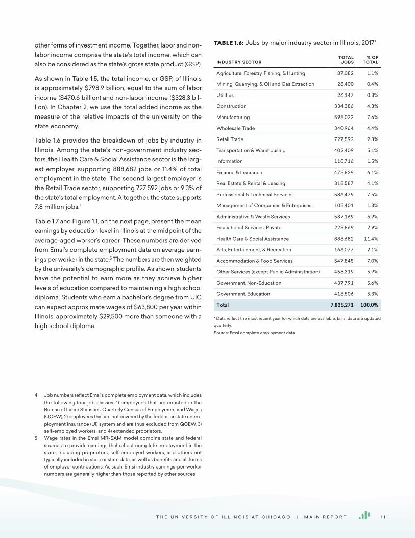
Table 1.6 provides the breakdown of jobs by industry in Illinois. Among the state’s non-government industry sec-tors, the Health Care & Social Assistance sector is the larg-est employer, supporting 888,682 jobs or 11.4% of total employment in the state. The second largest employer is the Retail Trade sector, supporting 727,592 jobs or 9.3% of the state’s total employment. Altogether, the state supports 7.8 million jobs.4

Table 1.7 and Figure 1.1, on the next page, present the mean earnings by education level in Illinois at the midpoint of the average-aged worker’s career. These numbers are derived from Emsi’s complete employment data on average earn-ings per worker in the state.5 The numbers are then weighted by the university’s demographic profile. As shown, students have the potential to earn more as they achieve higher levels of education compared to maintaining a high school diploma. Students who earn a bachelor’s degree from UIC can expect approximate wages of $63,800 per year within Illinois, approximately $29,500 more than someone with a high school diploma.

4 Job numbers reflect Emsi’s complete employment data, which includes the following four job classes: 1) employees that are counted in the Bureau of Labor Statistics’ Quarterly Census of Employment and Wages (QCEW), 2) employees that are not covered by the federal or state unem-ployment insurance (UI) system and are thus excluded from QCEW, 3) self-employed workers, and 4) extended proprietors.

5 Wage rates in the Emsi MR-SAM model combine state and federal sources to provide earnings that reflect complete employment in the state, including proprietors, self-employed workers, and others not typically included in state or state data, as well as benefits and all forms of employer contributions. As such, Emsi industry earnings-per-worker numbers are generally higher than those reported by other sources.

TABLE 1.6: Jobs by major industry sector in Illinois, 2017*

INDUSTRY SECTORTOTAL

JOBS% OF

TOTAL

Agriculture, Forestry, Fishing, & Hunting 87,082 1.1%

Mining, Quarrying, & Oil and Gas Extraction 28,400 0.4%

Utilities 26,147 0.3%

Construction 334,386 4.3%

Manufacturing 595,022 7.6%

Wholesale Trade 340,964 4.4%

Retail Trade 727,592 9.3%

Transportation & Warehousing 402,409 5.1%

Information 118,716 1.5%

Finance & Insurance 475,829 6.1%

Real Estate & Rental & Leasing 318,587 4.1%

Professional & Technical Services 586,479 7.5%

Management of Companies & Enterprises 105,401 1.3%

Administrative & Waste Services 537,169 6.9%

Educational Services, Private 223,869 2.9%

Health Care & Social Assistance 888,682 11.4%

Arts, Entertainment, & Recreation 166,077 2.1%

Accommodation & Food Services 547,845 7.0%

Other Services (except Public Administration) 458,319 5.9%

Government, Non-Education 437,791 5.6%

Government, Education 418,506 5.3%

Total 7,825,271 100.0%

* Data reflect the most recent year for which data are available. Emsi data are updated

quarterly.

Source: Emsi complete employment data.


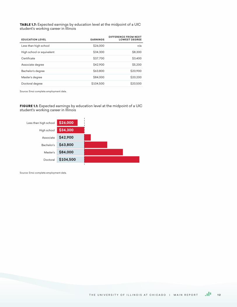
TABLE 1.7: Expected earnings by education level at the midpoint of a UIC student’s working career in Illinois

EDUCATION LEVEL EARNINGSDIFFERENCE FROM NEXT

LOWEST DEGREE

Less than high school $26,000 n/a

High school or equivalent $34,300 $8,300

Certificate $37,700 $3,400

Associate degree $42,900 $5,200

Bachelor’s degree $63,800 $20,900

Master’s degree $84,000 $20,200

Doctoral degree $104,500 $20,500


FIGURE 1.1: Expected earnings by education level at the midpoint of a UIC student’s working career in Illinois


25+33+41+61+80+100Less than high school

High school

Associate

Bachelor’s

Master’s

Doctoral

0+0+33+33+33+33 $26,000

$34,300

$42,900

$63,800

$84,000

$104,500


C H A P T E R 2 :

Economic Impacts on the Illinois Economy

UIC impacts the Illinois economy in a variety of ways. The university is an employer and buyer

of goods and services. It attracts monies that otherwise would not have entered the state

economy through its day-to-day and research operations, its hospital and entrepreneurial

activities, and the expenditures of its students and visitors. Further, it provides students with

the knowledge, skills, and abilities they need to become productive citizens and add to the

overall output of the state.

In this chapter, we estimate the following economic impacts of UIC: 1) the day-to-day operations spending impact; 2) the research spending impact; 3) the hospital spending impact; 4) the start-up company impact; 5) the student spending impact; 6) the visitor spending impact; and 7) the alumni impact, measuring the income added in the state as former students expand the state economy’s stock of human capital.

When exploring each of these economic impacts, we con-sider the following hypothetical question:

How would economic activity change in Illinois if UIC and all its alumni did not exist in FY 2017?

Each of the economic impacts should be interpreted according to this hypothetical question. Another way to think about the question is to realize that we measure net impacts, not gross impacts. Gross impacts represent an upper-bound estimate in terms of capturing all activity stemming from the university; however, net impacts reflect a truer measure since they demonstrate what would not have existed in the state economy if not for the university.

Economic impact analyses use different types of impacts to estimate the results. The impact focused on in this study assesses the change in income. This measure is similar to the commonly used gross state product (GSP). Income may be further broken out into the labor income impact, also known as earnings, which assesses the change in employee

compensation; and the non-labor income impact, which assesses the change in business profits. Together, labor income and non-labor income sum to total income.

Another way to state the impact is in terms of jobs, a mea-sure of the number of full- and part-time jobs that would be required to support the change in income. Finally, a frequently used measure is the sales impact, which com-prises the change in business sales revenue in the economy as a result of increased economic activity. It is important to bear in mind, however, that much of this sales revenue leaves the state economy through intermediary transac-tions and costs.6 All of these measures – added labor and non-labor income, total income, jobs, and sales – are used to estimate the economic impact results presented in this chapter. The analysis breaks out the impact measures into different components, each based on the economic effect that caused the impact. The following is a list of each type of effect presented in this analysis:

• The initial effect is the exogenous shock to the econ-omy caused by the initial spending of money, whether to pay for salaries and wages, purchase goods or services, or cover operating expenses.

• The initial round of spending creates more spending in the economy, resulting in what is commonly known as

6 See Appendix 3 for an example of the intermediary costs included in the sales impact but not in the income impact.


the multiplier effect. The multiplier effect comprises the additional activity that occurs across all industries in the economy and may be further decomposed into the following three types of effects:

· The direct effect refers to the additional economic activity that occurs as the industries affected by the initial effect spend money to purchase goods and services from their supply chain industries.

· The indirect effect occurs as the supply chain of the initial industries creates even more activity in the economy through their own inter-industry spending.

· The induced effect refers to the economic activity created by the household sector as the businesses affected by the initial, direct, and indirect effects raise salaries or hire more people.

The terminology used to describe the economic effects listed above differs slightly from that of other commonly used input-output models, such as IMPLAN. For example, the initial effect in this study is called the “direct effect” by IMPLAN, as shown in the table below. Further, the term “indirect effect” as used by IMPLAN refers to the combined direct and indirect effects defined in this study. To avoid confusion, readers are encouraged to interpret the results presented in this chapter in the context of the terms and definitions listed above. Note that, regardless of the effects used to decompose the results, the total impact measures are analogous.

Multiplier effects in this analysis are derived using Emsi’s MR-SAM input-output model that captures the intercon-nection of industries, government, and households in the state. The Emsi MR-SAM contains approximately 1,000 industry sectors at the highest level of detail available in the North American Industry Classification System (NAICS) and supplies the industry-specific multipliers required to determine the impacts associated with increased activity within a given economy. For more information on the Emsi MR-SAM model and its data sources, see Appendix 4.

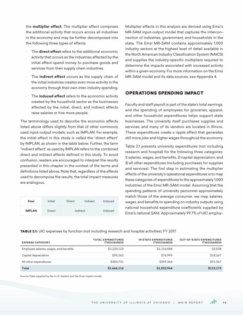
OPERATIONS SPENDING IMPACT

Faculty and staff payroll is part of the state’s total earnings, and the spending of employees for groceries, apparel, and other household expenditures helps support state businesses. The university itself purchases supplies and services, and many of its vendors are located in Illinois. These expenditures create a ripple effect that generates still more jobs and higher wages throughout the economy.

Table 2.1 presents university expenditures (not including research and hospital) for the following three categories: 1) salaries, wages, and benefits, 2) capital depreciation, and 3) all other expenditures (including purchases for supplies and services). The first step in estimating the multiplier effects of the university’s operational expenditures is to map these categories of expenditures to the approximately 1,000 industries of the Emsi MR-SAM model. Assuming that the spending patterns of university personnel approximately match those of the average consumer, we map salaries, wages, and benefits to spending on industry outputs using national household expenditure coefficients supplied by Emsi’s national SAM. Approximately 99.7% of UIC employ-

Emsi Initial Direct Indirect Induced

IMPLAN Direct Indirect Induced

TABLE 2.1: UIC expenses by function (not including research and hospital activities), FY 2017

EXPENSE CATEGORYTOTAL EXPENDITURES

(THOUSANDS)IN-STATE EXPENDITURES

(THOUSANDS)OUT-OF-STATE EXPENDITURES

(THOUSANDS)

Employee salaries, wages, and benefits $1,220,123 $1,216,584 $3,538

Capital depreciation $95,263 $76,995 $18,267

All other expenditures $350,731 $259,364 $91,367

Total $1,666,116 $1,552,944 $113,173

Source: Data supplied by the U of I System and the Emsi impact model.


ees work in Illinois (see Table 1.1), and therefore we consider 100% of the salaries, wages, and benefits. For the other two expenditure categories (i.e., capital depreciation and all other expenditures), we assume the university’s spend-ing patterns approximately match national averages and apply the national spending coefficients for NAICS 611310 (Colleges, Universities, and Professional Schools).7 Capital depreciation is mapped to the construction sectors of NAICS 611310 and the university’s remaining expenditures to the non-construction sectors of NAICS 611310.

We now have three vectors of expenditures for UIC: one for salaries, wages, and benefits; another for capital items; and a third for the university’s purchases of supplies and services. The next step is to estimate the portion of these expenditures that occur inside the state. The expenditures occurring outside the state are known as leakages. We estimate in-state expenditures using regional purchase coefficients (RPCs), a measure of the overall demand for the commodities produced by each sector that is satis-fied by state suppliers, for each of the approximately 1,000 industries in the MR-SAM model.8 For example, if 40% of the demand for NAICS 541211 (Offices of Certified Public Accountants) is satisfied by state suppliers, the RPC for that industry is 40%. The remaining 60% of the demand for NAICS 541211 is provided by suppliers located outside

7 See Appendix 1 for a definition of NAICS.8 See Appendix 4 for a description of Emsi’s MR-SAM model.

the state. The three vectors of expenditures are multiplied, industry by industry, by the corresponding RPC to arrive at the in-state expenditures associated with the university. See Table 2.1 for a break-out of the expenditures that occur in-state. Finally, in-state spending is entered, industry by industry, into the MR-SAM model’s multiplier matrix, which in turn provides an estimate of the associated multiplier effects on state labor income, non-labor income, total income, sales, and jobs.

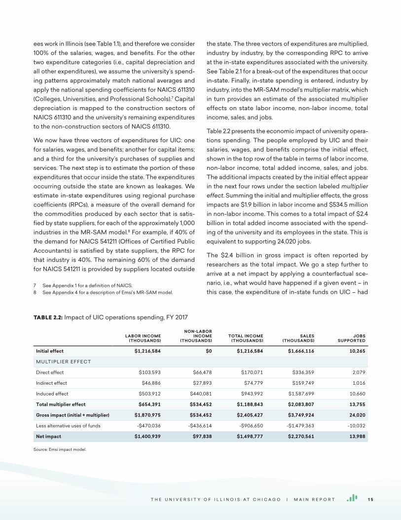
Table 2.2 presents the economic impact of university opera-tions spending. The people employed by UIC and their salaries, wages, and benefits comprise the initial effect, shown in the top row of the table in terms of labor income, non-labor income, total added income, sales, and jobs. The additional impacts created by the initial effect appear in the next four rows under the section labeled multiplier effect. Summing the initial and multiplier effects, the gross impacts are $1.9 billion in labor income and $534.5 million in non-labor income. This comes to a total impact of $2.4 billion in total added income associated with the spend-ing of the university and its employees in the state. This is equivalent to supporting 24,020 jobs.

The $2.4 billion in gross impact is often reported by researchers as the total impact. We go a step further to arrive at a net impact by applying a counterfactual sce-nario, i.e., what would have happened if a given event – in this case, the expenditure of in-state funds on UIC – had

TABLE 2.2: Impact of UIC operations spending, FY 2017

LABOR INCOME

(THOUSANDS)

NON-LABOR INCOME

(THOUSANDS)TOTAL INCOME

(THOUSANDS)SALES

(THOUSANDS)JOBS

SUPPORTED

Initial effect $1,216,584 $0 $1,216,584 $1,666,116 10,265

M U LT I P L I E R E F F E C T

Direct effect $103,593 $66,478 $170,071 $336,359 2,079

Indirect effect $46,886 $27,893 $74,779 $159,749 1,016

Induced effect $503,912 $440,081 $943,992 $1,587,699 10,660

Total multiplier effect $654,391 $534,452 $1,188,843 $2,083,807 13,755

Gross impact (initial + multiplier) $1,870,975 $534,452 $2,405,427 $3,749,924 24,020

Less alternative uses of funds -$470,036 -$436,614 -$906,650 -$1,479,363 -10,032

Net impact $1,400,939 $97,838 $1,498,777 $2,270,561 13,988

Source: Emsi impact model.


not occurred. UIC received an estimated 71% of its funding from sources within Illinois. These monies came from the tuition and fees paid by resident students, from the auxiliary revenue and donations from private sources located within the state, from state and local taxes, and from the financial aid issued to students by state and local government. We must account for the opportunity cost of this in-state fund-ing. Had other industries received these monies rather than UIC, income impacts would have still been created in the economy. In economic analysis, impacts that occur under counterfactual conditions are used to offset the impacts that actually occur in order to derive the true impact of the event under analysis.

We estimate this counterfactual by simulating a scenario where in-state monies spent on the university are instead spent on consumer goods and savings. This simulates the in-state monies being returned to the taxpayers and being spent by the household sector. Our approach is to establish the total amount spent by in-state students and taxpayers on UIC, map this to the detailed industries of the MR-SAM model using national household expenditure coefficients, use the industry RPCs to estimate in-state spending, and run the in-state spending through the MR-SAM model’s multiplier matrix to derive multiplier effects. The results of this exercise are shown as negative values in the row labeled less alternative uses of funds in Table 2.2.

The total net impacts of the university’s operations are equal to the gross impacts less the impacts of the alternative use of funds – the opportunity cost of the state and local money. As shown in the last row of Table 2.2, the total net impact is approximately $1.4 billion in labor income and $97.8 million in non-labor income. This sums together to $1.5 billion in total added income and is equivalent to 13,988 jobs. These impacts represent new economic activity created in the

state economy solely attributable to the operations of UIC.

RESEARCH SPENDING IMPACT

Similar to the day-to-day operations of UIC, research activi-ties impact the economy by employing people and requir-ing the purchase of equipment and other supplies and services. Table 2.3 shows UIC’s research expenses by func-tion – payroll, equipment, pass-throughs, and other – for the last four fiscal years. In FY 2017, UIC spent over $372.6 million on research and development activities. These expenses would not have been possible without funding from outside the state – UIC received around 53% of its research funding from federal and other sources.

We employ a methodology similar to the one used to estimate the impacts of operational expenses. We begin by mapping total research expenses to the industries of the MR-SAM model, removing the spending that occurs outside the state, and then running the in-state expenses through the multiplier matrix. As with the operations spend-ing impact, we also adjust the gross impacts to account for the opportunity cost of monies withdrawn from the state economy to support the research of UIC, whether through state-sponsored research awards or through private dona-tions. Again, we refer to this adjustment as the alternative use of funds.

Mapping the research expenses by category to the indus-tries of the MR-SAM model – the only difference from our previous methodology – requires some exposition. We asked the U of I System to provide information on expen-ditures by research and development field as they report to the National Science Foundation’s Higher Education

TABLE 2.3: Research expenses by function of UIC, FY 2017

FISCAL YEARPAYROLL

(THOUSANDS)EQUIPMENT

(THOUSANDS)PASS-THROUGHS

(THOUSANDS)OTHER

(THOUSANDS)TOTAL

(THOUSANDS)

2017 $180,556 $10,269 $22,676 $159,118 $372,619

2016 $168,888 $8,777 $22,539 $137,092 $337,296

2015 $176,088 $8,376 $23,088 $147,008 $354,560

2014 $164,728 $9,779 $25,137 $148,244 $347,888



Research and Development Survey (HERD).9 We map these fields of study to their respective industries in the MR-SAM model. The result is a distribution of research expenses to the various 1,000 industries that follows a weighted average of the fields of study reported by UIC.

Initial, direct, indirect, and induced effects of UIC’s research expenses appear in Table 2.4. As with the operations spend-ing impact, the initial effect consists of the 1,520 research jobs and their associated salaries, wages, and benefits. The university’s research expenses have a total gross impact of $392.4 million in labor income and $120.1 million in non-labor income. This sums together to $512.4 million in added

9 The fields include environmental sciences, life sciences, math and computer sciences, physical sciences, psychology, social sciences, sciences not elsewhere classified, engineering, and all non-science and engineering fields.

income, equivalent to 5,372 jobs. Taking into account the impact of the alternative uses of funds, net research expen-diture impacts of UIC are $346.8 million in labor income and $77.8 million in non-labor income. This sums together to $424.6 million in total added income and is equivalent to 4,370 jobs.

Research and innovation plays an important role in driving the Illinois economy. Some indicators of innovation are the number of invention disclosures, patent applications, and licenses and options executed. Over the last four years, UIC received 624 invention disclosures, filed 199 new U.S. patent applications, and produced 212 licenses (see Table 2.5). The university also received $109.6 million in gross license income (adjusted). Without the research activities of UIC, this level of innovation and sustained economic growth would not have been possible.

TABLE 2.4: Impact of UIC research spending, FY 2017

LABOR INCOME

(THOUSANDS)

NON-LABOR INCOME


(THOUSANDS)SALES

(THOUSANDS)JOBS

SUPPORTED

Initial effect $180,032 $0 $180,032 $372,619 1,520


Direct effect $62,630 $26,634 $89,264 $160,044 1,030

Indirect effect $26,446 $11,553 $37,999 $73,223 463

Induced effect $123,246 $81,898 $205,143 $347,541 2,360

Total multiplier effect $212,322 $120,084 $332,406 $580,808 3,853

Gross impact (initial + multiplier) $392,354 $120,084 $512,438 $953,427 5,372

Less alternative uses of funds -$45,565 -$42,316 -$87,881 -$144,185 -1,003

Net impact $346,789 $77,768 $424,557 $809,242 4,370


TABLE 2.5: Invention disclosures, patent applications, licenses, and license income of UIC

FISCAL YEARINVENTION DISCLOSURES

RECEIVEDPATENT APPLICATIONS

FILEDLICENSES AND

OPTIONS EXECUTEDADJUSTED GROSS

LICENSE INCOME

2017 148 48 52 $28,037,412

2016 138 45 56 $28,859,183

2015 169 46 52 $27,250,681

2014 169 60 52 $25,440,611

Total 624 199 212 $109,587,887



HOSPITAL SPENDING IMPACT

In this section we estimate the economic impact of the spending of the University of Illinois Hospital & Health Sciences System (UI Health), which would not exist with-out UIC. Note that the broader health-related impacts of healthcare provided through the hospital are beyond the scope of this analysis and are not included.

In FY 2017, $1.1 billion was spent on hospital operations for UI Health. To avoid any double counting, this spending was not included in the operations spending impact previously reported. Any medical research expenses from the hospital are accounted for in the research spending impact and are not included here.

The methodology used here is similar to that used when estimating the impacts of operations and research spend-ing. Salaries, wages, and benefits are mapped to industries using national household expenditure coefficients. Assum-

ing UI Health has a spending pattern similar to that of the national average of general and surgical hospitals, we map its capital and other expenses to the industries of the SAM model using coefficients for General Medical & Surgical Hospitals (NAICS 622110). Next, we remove the spending that occurs outside the state, and run the in-state expenses through the multiplier matrix. Unlike the previous section, we do not estimate the impacts that would have been cre-ated with an alternative use of these funds. This is because there is not a significant alternative to spending money on health care. Table 2.7 presents the impacts of UI Health’s hospital expenses.

The payroll and number of people employed by UI Health comprise the initial effect. The total impacts of hospital expenses (the sum of the initial and multiplier effects) are $1.1 billion in labor income and $379.2 million in non-labor income. This totals to $1.5 billion in total added income and is equivalent to supporting 14,348 jobs.

TABLE 2.7: Impact of UI Health expenses, FY 2017

LABOR INCOME

(THOUSANDS)

NON-LABOR INCOME


(THOUSANDS)SALES

(THOUSANDS)JOBS

SUPPORTED

Initial effect $592,259 $0 $592,259 $1,055,786 3,923


Direct effect $144,639 $81,197 $225,836 $378,111 2,482

Indirect effect $56,354 $30,718 $87,072 $155,696 1,019

Induced effect $346,433 $267,310 $613,743 $1,008,358 6,924

Total multiplier effect $547,426 $379,225 $926,650 $1,542,165 10,425

Total impact (initial + multiplier) $1,139,685 $379,225 $1,518,910 $2,597,951 14,348


TABLE 2.6: UI Health expenses by function, FY 2017

EXPENSE CATEGORYTOTAL EXPENSES

(THOUSANDS)IN-STATE EXPENSES

(THOUSANDS)OUT-OF-STATE EXPENSES

(THOUSANDS)

Salaries, wages and benefits $593,268 $592,259 $1,009

Capital depreciation $24,748 $17,183 $7,565

All other expenses $437,770 $360,927 $76,843

Total $1,055,786 $970,370 $85,416

Source: Data supplied by the U of I System and the Emsi impact model.


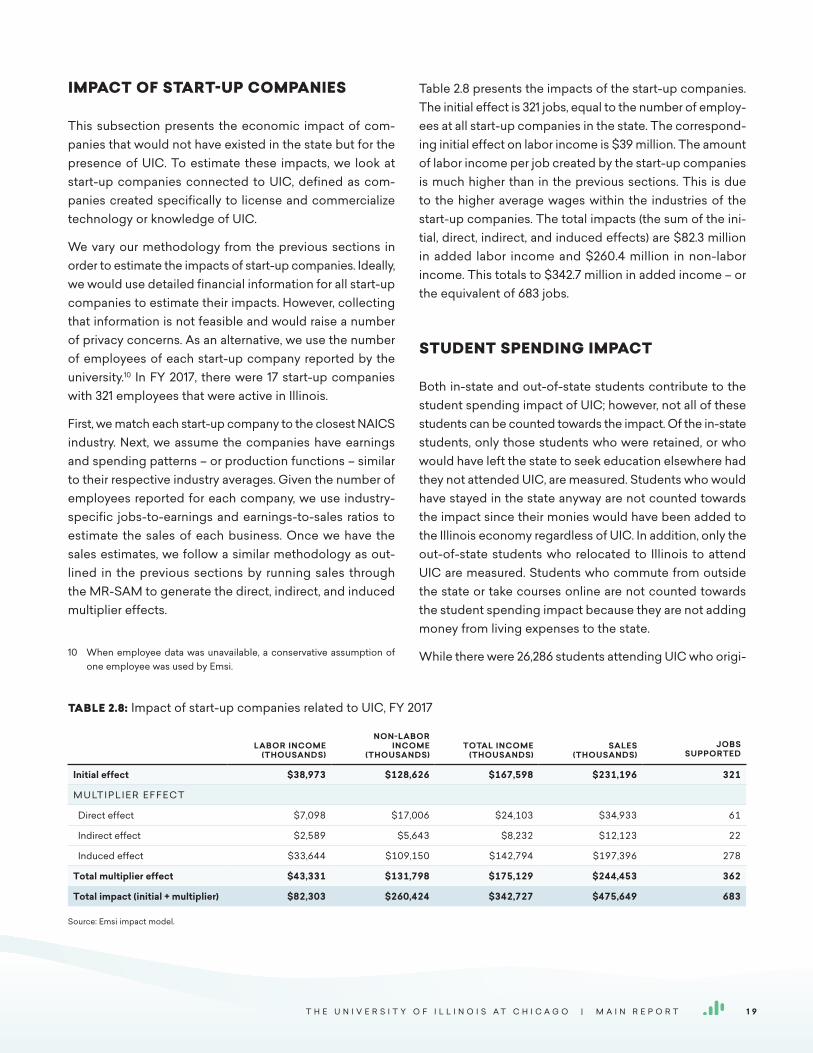
IMPACT OF START-UP COMPANIES

This subsection presents the economic impact of com-panies that would not have existed in the state but for the presence of UIC. To estimate these impacts, we look at start-up companies connected to UIC, defined as com-panies created specifically to license and commercialize technology or knowledge of UIC.

We vary our methodology from the previous sections in order to estimate the impacts of start-up companies. Ideally, we would use detailed financial information for all start-up companies to estimate their impacts. However, collecting that information is not feasible and would raise a number of privacy concerns. As an alternative, we use the number of employees of each start-up company reported by the university.10 In FY 2017, there were 17 start-up companies with 321 employees that were active in Illinois.

First, we match each start-up company to the closest NAICS industry. Next, we assume the companies have earnings and spending patterns – or production functions – similar to their respective industry averages. Given the number of employees reported for each company, we use industry-specific jobs-to-earnings and earnings-to-sales ratios to estimate the sales of each business. Once we have the sales estimates, we follow a similar methodology as out-lined in the previous sections by running sales through the MR-SAM to generate the direct, indirect, and induced multiplier effects.

10 When employee data was unavailable, a conservative assumption of one employee was used by Emsi.

Table 2.8 presents the impacts of the start-up companies. The initial effect is 321 jobs, equal to the number of employ-ees at all start-up companies in the state. The correspond-ing initial effect on labor income is $39 million. The amount of labor income per job created by the start-up companies is much higher than in the previous sections. This is due to the higher average wages within the industries of the start-up companies. The total impacts (the sum of the ini-tial, direct, indirect, and induced effects) are $82.3 million in added labor income and $260.4 million in non-labor income. This totals to $342.7 million in added income – or the equivalent of 683 jobs.

STUDENT SPENDING IMPACT

Both in-state and out-of-state students contribute to the student spending impact of UIC; however, not all of these students can be counted towards the impact. Of the in-state students, only those students who were retained, or who would have left the state to seek education elsewhere had they not attended UIC, are measured. Students who would have stayed in the state anyway are not counted towards the impact since their monies would have been added to the Illinois economy regardless of UIC. In addition, only the out-of-state students who relocated to Illinois to attend UIC are measured. Students who commute from outside the state or take courses online are not counted towards the student spending impact because they are not adding money from living expenses to the state.

While there were 26,286 students attending UIC who origi-

TABLE 2.8: Impact of start-up companies related to UIC, FY 2017

LABOR INCOME

(THOUSANDS)

NON-LABOR INCOME


(THOUSANDS)SALES

(THOUSANDS)JOBS

SUPPORTED

Initial effect $38,973 $128,626 $167,598 $231,196 321


Direct effect $7,098 $17,006 $24,103 $34,933 61

Indirect effect $2,589 $5,643 $8,232 $12,123 22

Induced effect $33,644 $109,150 $142,794 $197,396 278

Total multiplier effect $43,331 $131,798 $175,129 $244,453 362

Total impact (initial + multiplier) $82,303 $260,424 $342,727 $475,649 683



nated from Illinois (not including dual credit high school students), not all of them would have remained in the state if not for the existence of UIC. We apply a conservative assumption that 15% of these students would have left Illinois for other education opportunities if UIC did not exist.11 Therefore, we recognize that the in-state spending of 3,943 students retained in the state is attributable to UIC. These students, called retained students, spent money at businesses in the state for groceries, accommodation, transportation, and so on. Of the retained students, we estimate 386 lived on campus while attending UIC. While these students spend money while attending the university, we exclude most of their spending for room and board since these expenditures are already reflected in the impact of the university’s operations.

Relocated students are also accounted for in UIC’s student spending impact. An estimated 4,493 students came from outside the state and lived off campus while attending UIC in FY 2017. Another estimated 487 out-of-state students lived on campus while attending the university. We apply the same adjustment as described above to the students that relocated and lived on campus during their time at UIC. Collectively, the off-campus expenditures of out-of-state students supported jobs and created new income in the state economy.12

The average costs for students appear in the first section of Table 2.9, equal to $14,510 per student. Note that this table excludes expenses for books and supplies, since many of these monies are already reflected in the operations impact discussed in the previous section. We multiply the $14,510 in annual costs by the 8,050 students who either were retained or relocated to the state because of UIC and lived in-state but off campus. This provides us with an estimate of their total spending. For students living on campus, we multiply the per-student cost of personal expenses, transportation, and off-campus food purchases (assumed to be equal to 25% of room and board) by the number of students who lived in the state but on campus while attending (873 stu-dents). Altogether, off-campus spending of relocated and

11 See Chapter 4 for a sensitivity analysis of the retained student variable.12 Online students and students who commuted to Illinois from outside the

state are not considered in this calculation because it is assumed their living expenses predominantly occurred in the state where they resided during the analysis year. We recognize that not all online students live outside the state, but keep the assumption given data limitations.

retained students generated gross sales of $122.3 million. This figure, once net of the monies paid to student workers, yields net off-campus sales of $98.7 million, as shown in the bottom row of Table 2.9.

Estimating the impacts generated by the $98.7 million in student spending follows a procedure similar to that of the operations impact described above. We distribute the $98.7 million in sales to the industry sectors of the MR-SAM model, apply RPCs to reflect in-state spending, and run the net sales figures through the MR-SAM model to derive multiplier effects.

Table 2.10, on the next page, presents the results. Unlike the previous subsections, the initial effect is purely sales-ori-ented and there is no change in labor or non-labor income. The impact of relocated and retained student spending thus falls entirely under the multiplier effect. The total impact of student spending is $47.6 million in labor income and $39.6 million in non-labor income. This sums together to $87.2 million in total added income and is equivalent to support-ing 1,648 jobs. These values represent the direct effects created at the businesses patronized by the students, the indirect effects created by the supply chain of those busi-

TABLE 2.9: Average student costs and total sales generated by relocated and retained students in Illinois, FY 2017

Room and board $10,882

Personal expenses $2,254

Transportation $1,374

Total expenses per student $14,510

Number of students that were retained 3,943

Number of students that relocated 4,980

Gross retained student sales $54,063,438

Gross relocated student sales $68,283,182

Total gross off-campus sales $122,346,619

Wages and salaries paid to student workers* $23,598,209

Net off-campus sales $98,748,410

* This figure reflects only the portion of payroll that was used to cover the living expenses

of relocated and retained student workers who lived in the state.

Source: Student costs and wages provided by the U of I System. The number of relo-

cated and retained students who lived in the state off campus or on campus while

attending is derived by Emsi from the student origin data and in-term residence data

supplied by the U of I System.


nesses, and the effects of the increased spending of the household sector throughout the state economy as a result of the direct and indirect effects.

VISITOR SPENDING IMPACT

In addition to out-of-state students, thousands of visitors came to UIC to participate in various activities, including commencement, sports events, and orientation. The U of I System estimated that 8,020 out-of-state visitors attended events hosted by UIC in FY 2017. Table 2.11 presents the average expenditures per person-trip for accommodation, food, transportation, and other personal expenses (includ-ing shopping and entertainment). Based on these figures, the gross spending of out-of-state visitors totaled $5 mil-

TABLE 2.10: Student spending impact, FY 2017

LABOR INCOME

(THOUSANDS)

NON-LABOR INCOME


(THOUSANDS)SALES

(THOUSANDS)JOBS

SUPPORTED

Initial effect $0 $0 $0 $98,748 0


Direct effect $21,121 $17,736 $38,857 $63,326 732

Indirect effect $7,237 $5,914 $13,151 $21,686 249

Induced effect $19,263 $15,968 $35,231 $57,011 668

Total multiplier effect $47,622 $39,618 $87,239 $142,023 1,648

Total impact (initial + multiplier) $47,622 $39,618 $87,239 $240,771 1,648


TABLE 2.12: Impact of the spending of UIC out-of-state visitors, FY 2017

LABOR INCOME

(THOUSANDS)

NON-LABOR INCOME


(THOUSANDS)SALES

(THOUSANDS)JOBS

SUPPORTED

Initial effect $0 $0 $0 $3,957 0


Direct effect $1,036 $718 $1,753 $3,082 36

Indirect effect $409 $278 $687 $1,222 15

Induced effect $923 $632 $1,555 $2,705 32

Total multiplier effect $2,368 $1,628 $3,995 $7,010 83

Total impact (initial + multiplier) $2,368 $1,628 $3,995 $10,967 83


TABLE 2.11: Average per-trip visitor costs and sales generated by out-of-state visitors in Illinois, FY 2017

Accommodation $159

Food $195

Entertainment and shopping $195

Transportation $72

Total expenses per visitor $620

Number of out-of-state visitors 8,020

Gross sales $4,971,812

On-campus sales (excluding text books) $1,014,484

Net off-campus sales $3,957,328

Source: Sales calculations by Emsi estimated based on data provided by the U of I

System.


lion in FY 2017. However, some of this spending includes monies paid to the university through non-textbook items (e.g., event tickets, food, etc.). These have already been accounted for in the operations impact and should thus be removed to avoid double-counting. We estimate that on-campus sales generated by out-of-state visitors totaled $1 million. The net sales from out-of-state visitors in FY 2017 thus come to $4 million.

Calculating the increase in income as a result of visitor spending again requires use of the MR-SAM model. The analysis begins by discounting the off-campus sales gen-erated by out-of-state visitors to account for leakage in the trade sector, and then bridging the net figures to the detailed sectors of the MR-SAM model. The model runs the net sales figures through the multiplier matrix to arrive at the multiplier effects. As shown in Table 2.12, the net impact of visitor spending in FY 2017 comes to $2.4 million in labor income and $1.6 million in non-labor income. This totals to $4 million in added income and is equivalent to supporting 83 jobs.

ALUMNI IMPACT

In this section, we estimate the economic impacts stem-ming from the added labor income of alumni in combination with their employers’ added non-labor income. This impact is based on the number of students who have attended UIC throughout its history. We then use this total number to consider the impact of those students in the single FY 2017. Former students who achieved a degree as well as those who may not have finished their degree or did not take courses for credit are considered alumni.

While UIC creates an economic impact through its opera-tions, research, hospital, entrepreneurial, student, and visitor spending, the greatest economic impact of UIC stems from the added human capital – the knowledge, creativity, imagi-nation, and entrepreneurship – found in its alumni. While attending UIC, students receive experience, education, and the knowledge, skills, and abilities that increase their productivity and allow them to command a higher wage once they enter the workforce. But the reward of increased productivity does not stop there. Talented professionals make capital more productive too (e.g., buildings, produc-tion facilities, equipment). The employers of UIC alumni

enjoy the fruits of this increased productivity in the form of additional non-labor income (i.e., higher profits).

The methodology here differs from the previous impacts in one fundamental way. Whereas the previous spending impacts depend on an annually renewed injection of new sales into the state economy, the alumni impact is the result of years of past instruction and the associated accumulation of human capital. The initial effect of alumni is comprised of two main components. The first and largest of these is the added labor income of UIC’s former students. The second component of the initial effect is comprised of the added non-labor income of the businesses that employ former students of UIC.

We begin by estimating the portion of alumni who are employed in the workforce. To estimate the historical employment patterns of alumni in the state, we use the following sets of data or assumptions: 1) settling-in factors to determine how long it takes the average student to settle into a career;13 2) death, retirement, and unemployment rates from the National Center for Health Statistics, the Social Security Administration, and the Bureau of Labor Statistics; and 3) state migration data from the Census Bureau. The result is the estimated portion of alumni from each previous year who were still actively employed in the state as of FY 2017.

The next step is to quantify the skills and human capital that alumni acquired from the university. We use the students’ production of CHEs as a proxy for accumulated human capital. The average number of CHEs completed per stu-dent in FY 2017 was 21.6. To estimate the number of CHEs present in the workforce during the analysis year, we use the university’s historical student headcount over the past 30 years, from FY 1988 to FY 2017.14 We multiply the 21.6 aver-age CHEs per student by the headcounts that we estimate are still actively employed from each of the previous years.15

13 Settling-in factors are used to delay the onset of the benefits to students in order to allow time for them to find employment and settle into their careers. In the absence of hard data, we assume a range between one and three years for students who graduate with a certificate or a degree, and between one and five years for returning students.

14 We apply a 30-year time horizon because the data on students who attended UIC prior to FY 1987-88 is less reliable, and because most of the students served more than 30 years ago had left the state workforce by FY 2017.

15 This assumes the average credit load and level of study from past years is equal to the credit load and level of study of students today.


Students who enroll at the university more than one year are counted at least twice in the historical enrollment data. However, CHEs remain distinct regardless of when and by whom they were earned, so there is no duplication in the CHE counts. We estimate there are approximately 10.7 mil-lion CHEs from alumni active in the workforce.

Next, we estimate the value of the CHEs, or the skills and human capital acquired by UIC alumni. This is done using the incremental added labor income stemming from the students’ higher wages. The incremental added labor income is the difference between the wage earned by UIC alumni and the alternative wage they would have earned had they not attended UIC. Using the state incremental earnings, credits required, and distribution of credits at each level of study, we estimate the average value per CHE to equal $265. This value represents the state average incremental increase in wages that alumni of UIC received during the analysis year for every CHE they completed.

Because workforce experience leads to increased produc-tivity and higher wages, the value per CHE varies depending on the students’ workforce experience, with the highest value applied to the CHEs of students who had been employed the longest by FY 2017, and the lowest value per CHE applied to students who were just entering the workforce. More information on the theory and calculations behind the value per CHE appears in Appendix 5. In deter-mining the amount of added labor income attributable to alumni, we multiply the CHEs of former students in each year of the historical time horizon by the corresponding average value per CHE for that year, and then sum the products together. This calculation yields approximately $2.8 billion in gross labor income from increased wages received by former students in FY 2017 (as shown in Table 2.13).

The next two rows in Table 2.13 show two adjustments used to account for counterfactual outcomes. As discussed above, counterfactual outcomes in economic analysis rep-resent what would have happened if a given event had not occurred. The event in question is the education and train-ing provided by UIC and subsequent influx of skilled labor into the state economy. The first counterfactual scenario that we address is the adjustment for alternative educa-tion opportunities. In the counterfactual scenario where UIC does not exist, we assume a portion of UIC alumni would have received a comparable education elsewhere

in the state or would have left the state and received a comparable education and then returned to the state. The incremental added labor income that accrues to those stu-dents cannot be counted towards the added labor income from UIC alumni. The adjustment for alternative education opportunities amounts to a 15% reduction of the $2.8 billion in added labor income.16 This means that 15% of the added labor income from UIC alumni would have been generated in the state anyway, even if the university did not exist. For more information on the alternative education adjustment, see Appendix 6.

The other adjustment in Table 2.13 accounts for the importa-tion of labor. Suppose UIC did not exist and in consequence there were fewer skilled workers in the state. Businesses could still satisfy some of their need for skilled labor by recruiting from outside Illinois. We refer to this as the labor import effect. Lacking information on its possible magni-tude, we assume 50% of the jobs that students fill at state businesses could have been filled by workers recruited from outside the state if the university did not exist.17 Con-sequently, the gross labor income must be adjusted to account for the importation of this labor, since it would have happened regardless of the presence of the university. We conduct a sensitivity analysis for this assumption in Chapter 4. With the 50% adjustment, the net added labor income added to the economy comes to $1.2 billion, as shown in Table 2.13.

16 For a sensitivity analysis of the alternative education opportunities vari-able, see Chapter 4.

17 A similar assumption is used by Walden (2014) in his analysis of the Cooperating Raleigh Colleges.

TABLE 2.13: Number of CHEs in workforce and initial labor income created in Illinois, FY 2017

Number of CHEs in workforce 10,669,195

Average value per CHE $265

Initial labor income, gross $2,823,493,815

C O U N T E R FAC T UA L S

Percent reduction for alternative education opportunities 15%

Percent reduction for adjustment for labor import effects 50%

Initial labor income, net $1,199,984,871



The $1.2 billion in added labor income appears under the initial effect in the labor income column of Table 2.14. To this we add an estimate for initial non-labor income. As discussed earlier in this section, businesses that employ former students of UIC see higher profits as a result of the increased productivity of their capital assets. To estimate this additional income, we allocate the initial increase in labor income ($1.2 billion) to the six-digit NAICS industry sectors where students are most likely to be employed. This allocation entails a process that maps completers in the state to the detailed occupations for which those completers have been trained, and then maps the detailed occupations to the six-digit industry sectors in the MR-SAM model.18 Using a crosswalk created by National Center for Education Statistics (NCES) and the Bureau of Labor Statis-tics, we map the breakdown of the university’s completers to the approximately 700 detailed occupations in the Standard Occupational Classification (SOC) system. Finally, we apply a matrix of wages by industry and by occupation from the MR-SAM model to map the occupational distribution of the $1.2 billion in initial labor income effects to the detailed industry sectors in the MR-SAM model.19

18 Completer data comes from the Integrated Postsecondary Education Data System (IPEDS), which organizes program completions according to the Classification of Instructional Programs (CIP) developed by the National Center for Education Statistics (NCES).

19 For example, if the MR-SAM model indicates that 20% of wages paid to workers in SOC 51-4121 (Welders) occur in NAICS 332313 (Plate Work Manufacturing), then we allocate 20% of the initial labor income effect under SOC 51-4121 to NAICS 332313.

Once these allocations are complete, we apply the ratio of non-labor to labor income provided by the MR-SAM model for each sector to our estimate of initial labor income. This computation yields an estimated $493 million in added non-labor income attributable to the university’s alumni. Sum-ming initial labor and non-labor income together provides the total initial effect of alumni productivity in the Illinois economy, equal to approximately $1.7 billion. To estimate multiplier effects, we convert the industry-specific income figures generated through the initial effect to sales using sales-to-income ratios from the MR-SAM model. We then run the values through the MR-SAM’s multiplier matrix.

Table 2.14 shows the multiplier effects of alumni. Multiplier effects occur as alumni generate an increased demand for consumer goods and services through the expenditure of their higher wages. Further, as the industries where alumni are employed increase their output, there is a correspond-ing increase in the demand for input from the industries in the employers’ supply chain. Together, the incomes gen-erated by the expansions in business input purchases and household spending constitute the multiplier effect of the increased productivity of the university’s alumni. The final results are $1.5 billion in added labor income and $556.6 million in added non-labor income, for an overall total of $2.1 billion in multiplier effects. The grand total of the alumni impact thus comes to $3.8 billion in total added income, the sum of all initial and multiplier labor and non-labor income effects. This is equivalent to supporting 38,440 jobs.

TABLE 2.14: Alumni impact, FY 2017

LABOR INCOME

(THOUSANDS)

NON-LABOR INCOME


(THOUSANDS)SALES

(THOUSANDS)JOBS

SUPPORTED

Initial effect $1,199,985 $492,971 $1,692,955 $3,781,560 16,730


Direct effect $276,617 $107,655 $384,272 $751,750 3,926

Indirect effect $116,459 $44,254 $160,713 $312,191 1,687

Induced effect $1,119,273 $404,703 $1,523,976 $2,864,288 16,096

Total multiplier effect $1,512,348 $556,612 $2,068,960 $3,928,229 21,710

Total impact (initial + multiplier) $2,712,333 $1,049,582 $3,761,916 $7,709,789 38,440



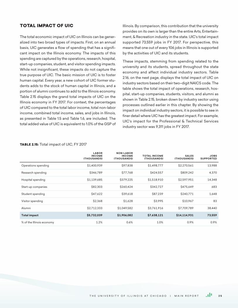
TOTAL IMPACT OF UIC

The total economic impact of UIC on Illinois can be gener-alized into two broad types of impacts. First, on an annual basis, UIC generates a flow of spending that has a signifi-cant impact on the Illinois economy. The impacts of this spending are captured by the operations, research, hospital, start-up companies, student, and visitor spending impacts. While not insignificant, these impacts do not capture the true purpose of UIC. The basic mission of UIC is to foster human capital. Every year, a new cohort of UIC former stu-dents adds to the stock of human capital in Illinois, and a portion of alumni continues to add to the Illinois economy. Table 2.15 displays the grand total impacts of UIC on the Illinois economy in FY 2017. For context, the percentages of UIC compared to the total labor income, total non-labor income, combined total income, sales, and jobs in Illinois, as presented in Table 1.5 and Table 1.6, are included. The total added value of UIC is equivalent to 1.0% of the GSP of

Illinois. By comparison, this contribution that the university provides on its own is larger than the entire Arts, Entertain-ment, & Recreation industry in the state. UIC’s total impact supported 73,559 jobs in FY 2017. For perspective, this means that one out of every 106 jobs in Illinois is supported by the activities of UIC and its students.

These impacts, stemming from spending related to the university and its students, spread throughout the state economy and affect individual industry sectors. Table 2.16, on the next page, displays the total impact of UIC on industry sectors based on their two–digit NAICS code. The table shows the total impact of operations, research, hos-pital, start-up companies, students, visitors, and alumni as shown in Table 2.15, broken down by industry sector using processes outlined earlier in this chapter. By showing the impact on individual industry sectors, it is possible to see in finer detail where UIC has the greatest impact. For example, UIC’s impact for the Professional & Technical Services industry sector was 9,311 jobs in FY 2017.

TABLE 2.15: Total impact of UIC, FY 2017

LABOR INCOME

(THOUSANDS)

NON-LABOR INCOME


(THOUSANDS)SALES

(THOUSANDS)JOBS

SUPPORTED

Operations spending $1,400,939 $97,838 $1,498,777 $2,270,561 13,988

Research spending $346,789 $77,768 $424,557 $809,242 4,370

Hospital spending $1,139,685 $379,225 $1,518,910 $2,597,951 14,348

Start-up companies $82,303 $260,424 $342,727 $475,649 683

Student spending $47,622 $39,618 $87,239 $240,771 1,648

Visitor spending $2,368 $1,628 $3,995 $10,967 83

Alumni $2,712,333 $1,049,582 $3,761,916 $7,709,789 38,440

Total impact $5,732,039 $1,906,082 $7,638,121 $14,114,931 73,559

% of the Illinois economy 1.2% 0.6% 1.0% 0.9% 0.9%


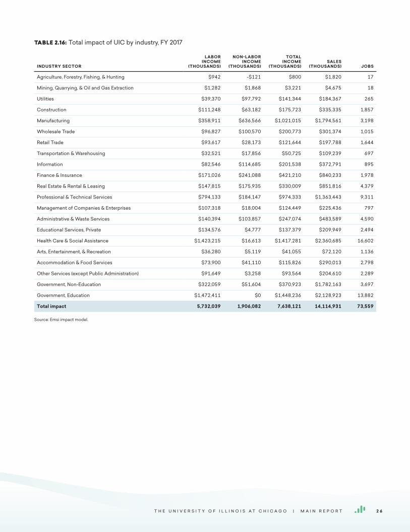
TABLE 2.16: Total impact of UIC by industry, FY 2017

INDUSTRY SECTOR

LABOR INCOME

(THOUSANDS)

NON-LABOR INCOME

(THOUSANDS)

TOTAL INCOME

(THOUSANDS)SALES

(THOUSANDS) JOBS

Agriculture, Forestry, Fishing, & Hunting $942 -$121 $800 $1,820 17

Mining, Quarrying, & Oil and Gas Extraction $1,282 $1,868 $3,221 $4,675 18

Utilities $39,370 $97,792 $141,344 $184,367 265

Construction $111,248 $63,182 $175,723 $335,335 1,857

Manufacturing $358,911 $636,566 $1,021,015 $1,794,561 3,198

Wholesale Trade $96,827 $100,570 $200,773 $301,374 1,015

Retail Trade $93,617 $28,173 $121,644 $197,788 1,644

Transportation & Warehousing $32,521 $17,856 $50,725 $109,239 697

Information $82,546 $114,685 $201,538 $372,791 895

Finance & Insurance $171,026 $241,088 $421,210 $840,233 1,978

Real Estate & Rental & Leasing $147,815 $175,935 $330,009 $851,816 4,379

Professional & Technical Services $794,133 $184,147 $974,333 $1,363,443 9,311

Management of Companies & Enterprises $107,318 $18,004 $124,449 $225,436 797

Administrative & Waste Services $140,394 $103,857 $247,074 $483,589 4,590

Educational Services, Private $134,576 $4,777 $137,379 $209,949 2,494

Health Care & Social Assistance $1,423,215 $16,613 $1,417,281 $2,360,685 16,602

Arts, Entertainment, & Recreation $36,280 $5,119 $41,055 $72,120 1,136

Accommodation & Food Services $73,900 $41,110 $115,826 $290,013 2,798

Other Services (except Public Administration) $91,649 $3,258 $93,564 $204,610 2,289

Government, Non-Education $322,059 $51,604 $370,923 $1,782,163 3,697

Government, Education $1,472,411 $0 $1,448,236 $2,128,923 13,882

Total impact 5,732,039 1,906,082 7,638,121 14,114,931 73,559



C H A P T E R 3 :

Investment Analysis

The benefits generated by UIC affect the lives of many people. The most obvious benefi-

ciaries are the university’s students; they give up time and money to go to the university in

return for a lifetime of higher wages and improved quality of life. But the benefits do not stop

there. As students earn more, communities and citizens throughout Illinois benefit from an

enlarged economy and a reduced demand for social services. In the form of increased tax

revenues and public sector savings, the benefits of education extend as far as the state and

local government.

Investment analysis is the process of evaluating total costs and measuring these against total benefits to determine whether or not a proposed venture will be profitable. If benefits outweigh costs, then the investment is worthwhile. If costs outweigh benefits, then the investment will lose money and is thus considered infeasible. In this chapter, we consider UIC as a worthwhile investment from the perspec-tives of students and society. In addition, we measure the benefits received by state and local taxpayers.

STUDENT PERSPECTIVE

To enroll in postsecondary education, students pay money for tuition and forego monies that otherwise they would have earned had they chosen to work instead of learn. From the perspective of students, education is the same as an investment; i.e., they incur a cost, or put up a certain amount of money, with the expectation of receiving benefits in return. The total costs consist of the monies that students pay in the form of tuition and fees and the opportunity costs of foregone time and money. The benefits are the higher earnings that students receive as a result of their education.

Calculating student costs

Student costs consist of three main items: direct outlays, opportunity costs, and future principal and interest costs

incurred from student loans. Direct outlays include tuition and fees, equal to $378.8 million from Table 1.2. Direct outlays also include the cost of books and supplies. On average, full-time students spent $1,400 each on books and supplies during the reporting year.20 Multiplying this figure times the number of full-time equivalents (FTEs) produced by UIC in FY 201721 generates a total cost of $32.2 million for books and supplies.

In order to pay the cost of tuition, many students had to take out loans. These students not only incur the cost of tuition from the university but also incur the interest cost of taking out loans. In FY 2017, students received a total of $51.1 million in federal loans to attend UIC.22 Students pay back these loans along with interest over the span of several years in the future. Since students pay off these loans over time, they accrue no initial cost during the analysis year. Hence, to avoid double counting, the $51.1 million in federal loans is subtracted from the costs incurred by students in FY 2017.

In addition to the cost of tuition, books, and supplies, stu-dents also experience an opportunity cost of attending college during the analysis year. Opportunity cost is the most difficult component of student costs to estimate.

20 Based on the data supplied by the U of I System.21 A single FTE is equal to 30 CHEs, so there were 22,969 FTEs produced

by students in FY 2017, equal to 689,080 CHEs divided by 30.22 Due to data limitations, only federal loans are considered in this analysis.


It measures the value of time and earnings foregone by students who go to the university rather than work. To calculate it, we need to know the difference between the students’ full earning potential and what they actually earn while attending the university.

We derive the students’ full earning potential by weighting the average annual earnings levels in Table 1.7 according to the education level breakdown of the student population when they first enrolled.23 However, the earnings levels in Table 1.7 reflect what average workers earn at the midpoint of their careers, not while attending the university. Because of this, we adjust the earnings levels to the average age of the student population (24) to better reflect their wages at their current age.24 This calculation yields an average full earning potential of $24,732 per student.

In determining how much students earn while enrolled in postsecondary education, an important factor to consider is the time that they actually spend on postsecondary edu-cation, since this is the only time that they are required to give up a portion of their earnings. We use the students’ CHE production as a proxy for time, under the assumption that the more CHEs students earn, the less time they have to work, and, consequently, the greater their foregone earn-ings. Overall, students attending UIC earned an average of 21.7 CHEs per student (excluding dual credit high school students), which is approximately equal to 72% of a full academic year.25 We thus include no more than $17,856 (or 72%) of the students’ full earning potential in the opportunity cost calculations.

Another factor to consider is the students’ employment status while enrolled in postsecondary education. It is esti-mated that 75% of students are employed.26 For the remain-der of students, we assume that they are either seeking work or planning to seek work once they complete their educa-tional goals. By choosing to enroll, therefore, non-working students give up everything that they can potentially earn

23 This is based on students who reported their prior level of education to UIC. The prior level of education data was then adjusted to exclude dual credit high school students.

24 Further discussion on this adjustment appears in Appendix 5.25 Equal to 30 CHEs divided by 30 for undergraduate students and 24 for

graduate students, the assumed number of CHEs in a full-time academic year.

26 Emsi provided an estimate of the percentage of students employed because the U of I System was unable to provide data.

during the academic year (i.e., the $17,856). The total value of their foregone earnings thus comes to $142.3 million.

Working students are able to maintain all or part of their earnings while enrolled. However, many of them hold jobs that pay less than statistical averages, usually because those are the only jobs they can find that accommodate their course schedule. These jobs tend to be at entry level, such as restaurant servers or cashiers. To account for this, we assume that working students hold jobs that pay 69% of what they would have earned had they chosen to work full-time rather than go to college.27 The remaining 31% comprises the percentage of their full earning potential that they forego. Obviously this assumption varies by person; some students forego more and others less. Since we do not know the actual jobs that students hold while attending, the 31% in foregone earnings serves as a reasonable average.

Working students also give up a portion of their leisure time in order to attend higher education institutions. Accord-ing to the Bureau of Labor Statistics American Time Use Survey, students forego up to 0.5 hours of leisure time per day.28 Assuming that an hour of leisure is equal in value to an hour of work, we derive the total cost of leisure by mul-tiplying the number of leisure hours foregone during the academic year by the average hourly pay of the students’ full earning potential. For working students, therefore, their total opportunity cost comes to $162.2 million, equal to the sum of their foregone earnings ($134.1 million) and foregone leisure time ($28.1 million).

Thus far we have discussed student costs during the analy-sis year. However, recall that students take out student loans to attend college during the year, which they will have to pay back over time. The amount they will be pay-ing in the future must be a part of their decision to attend the university today. Students who take out loans are not only required to pay back the principal of the loan but to also pay back a certain amount in interest. The first step in calculating students’ loan interest cost is to determine the payback time for the loans. The $51.1 million in loans was

27 The 69% assumption is based on the average hourly wage of jobs com-monly held by working students divided by the national average hourly wage. Occupational wage estimates are published by the Bureau of Labor Statistics (see http://www.bls.gov/oes/current/oes_nat.htm).

28 “Charts by Topic: Leisure and Sports Activities,” American Time Use Survey, Last modified December 2016, Accessed January 2017, http://www.bls.gov/TUS/CHARTS/LEISURE.HTM.


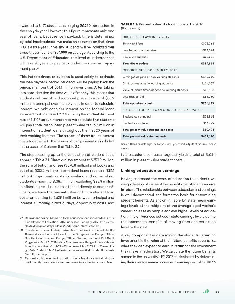
awarded to 8,172 students, averaging $6,250 per student in the analysis year. However, this figure represents only one year of loans. Because loan payback time is determined by total indebtedness, we make an assumption that since UIC is a four-year university, students will be indebted four times that amount, or $24,999 on average. According to the U.S. Department of Education, this level of indebtedness will take 20 years to pay back under the standard repay-ment plan.29

This indebtedness calculation is used solely to estimate the loan payback period. Students will be paying back the principal amount of $51.1 million over time. After taking into consideration the time value of money, this means that students will pay off a discounted present value of $33.9 million in principal over the 20 years. In order to calculate interest, we only consider interest on the federal loans awarded to students in FY 2017. Using the student discount rate of 3.8%30 as our interest rate, we calculate that students will pay a total discounted present value of $16.6 million in interest on student loans throughout the first 20 years of their working lifetime. The stream of these future interest costs together with the stream of loan payments is included in the costs of Column 5 of Table 3.2.

The steps leading up to the calculation of student costs appear in Table 3.1. Direct outlays amount to $359.9 million, the sum of tuition and fees ($378.8 million) and books and supplies ($32.2 million), less federal loans received ($51.1 million). Opportunity costs for working and non-working students amount to $218.7 million, excluding $85.8 million in offsetting residual aid that is paid directly to students.31 Finally, we have the present value of future student loan costs, amounting to $629.1 million between principal and interest. Summing direct outlays, opportunity costs, and

29 Repayment period based on total education loan indebtedness, U.S. Department of Education, 2017. Accessed February 2017. https://stu-dentaid.ed.gov/sa/repay-loans/understand/plans/standard.

30 The student discount rate is derived from the baseline forecasts for the 10-year discount rate published by the Congressional Budget Office. See the Congressional Budget Office, Student Loan and Pell Grant Programs - March 2012 Baseline, Congressional Budget Office Publica-tions, last modified March 13, 2012, accessed July 2013, http://www.cbo.gov/sites/default/files/cbofiles/attachments/43054_StudentLoanPell-GrantPrograms.pdf.

31 Residual aid is the remaining portion of scholarship or grant aid distrib-uted directly to a student after the university applies tuition and fees.

future student loan costs together yields a total of $629.1 million in present value student costs.

Linking education to earnings

Having estimated the costs of education to students, we weigh these costs against the benefits that students receive in return. The relationship between education and earnings is well documented and forms the basis for determining student benefits. As shown in Table 1.7, state mean earn-ings levels at the midpoint of the average-aged worker’s career increase as people achieve higher levels of educa-tion. The differences between state earnings levels define the incremental benefits of moving from one education level to the next.

A key component in determining the students’ return on investment is the value of their future benefits stream; i.e., what they can expect to earn in return for the investment they make in education. We calculate the future benefits stream to the university’s FY 2017 students first by determin-ing their average annual increase in earnings, equal to $187.6

TABLE 3.1: Present value of student costs, FY 2017 (thousands)

D I R E C T O U T L AY S I N F Y 2017

Tuition and fees $378,768

Less federal loans received -$51,074

Books and supplies $32,222

Total direct outlays $359,916

O P P O RT U N I T Y C O S T S I N F Y 2017

Earnings foregone by non-working students $142,310

Earnings foregone by working students $134,087

Value of leisure time foregone by working students $28,103

Less residual aid -$85,780

Total opportunity costs $218,719

F U T U R E S T U D E N T LOA N C O S T S ( P R E S E N T VA L U E)

Student loan principal $33,865

Student loan interest $16,629

Total present value student loan costs $50,494

Total present value student costs $629,130

Source: Based on data supplied by the U of I System and outputs of the Emsi impact

model.


million. This value represents the higher wages that accrues to students at the midpoint of their careers and is calculated based on the marginal wage increases of the CHEs that students complete while attending the university. Using the state of Illinois earnings, the marginal wage increase per CHE is $272. For a full description of the methodology used to derive the $187.6 million, see Appendix 5.

The second step is to project the $187.6 million annual increase in earnings into the future, for as long as stu-dents remain in the workforce. We do this using the Mincer function to predict the change in earnings at each point in an individual’s working career. 32 The Mincer function originated from Mincer’s seminal work on human capital (1958). The function estimates earnings using an individual’s years of education and post-schooling experience. While some have criticized Mincer’s earnings function, it is still upheld in recent data and has served as the foundation for a variety of research pertaining to labor economics. Card (1999 and 2001) addresses a number of these criticisms using U.S. based research over the last three decades and concludes that any upward bias in the Mincer parameters is on the order of 10% or less. We use state-specific and education level-specific Mincer coefficients. To account for any upward bias, we incorporate a 10% reduction in our projected earnings, otherwise known as the ability bias. With the $187.6 million representing the students’ higher earn-ings at the midpoint of their careers, we apply scalars from the Mincer function to yield a stream of projected future benefits that gradually increase from the time students enter the workforce, peak shortly after the career midpoint, and then dampen slightly as students approach retirement at age 67. This earnings stream appears in Column 2 of Table 3.2, on the next page.

As shown in Table 3.2, the $187.6 million in gross higher earnings occurs around Year 15, which is the approximate midpoint of the students’ future working careers given the average age of the student population and an assumed retirement age of 67. In accordance with the Mincer func-tion, the gross higher earnings that accrues to students in the years leading up to the midpoint is less than $187.6 million and the gross higher earnings in the years after the midpoint is greater than $187.6 million.

32 Appendix 5 provides more information on the Mincer function and how it is used to predict future earnings growth.

The final step in calculating the students’ future benefits stream is to net out the potential benefits generated by students who are either not yet active in the workforce or who leave the workforce over time. This adjustment appears in Column 3 of Table 3.2 and represents the percentage of the FY 2017 student population that will be employed in the workforce in a given year. Note that the percentages in the first five years of the time horizon are relatively lower than those in subsequent years. This is because many students delay their entry into the workforce, either because they are still enrolled at the university or because they are unable to find a job immediately upon graduation. Accordingly, we apply a set of “settling-in” factors to account for the time needed by students to find employment and settle into their careers. As discussed in Chapter 2, settling-in factors delay the onset of the benefits by one to three years for students who graduate with a certificate or a degree and by one to five years for degree-seeking students who do not complete during the analysis year.

Beyond the first five years of the time horizon, students will leave the workforce for any number of reasons, whether death, retirement, or unemployment. We estimate the rate of attrition using the same data and assumptions applied in the calculation of the attrition rate in the economic impact analysis of Chapter 2.33 The likelihood of leaving the work-force increases as students age, so the attrition rate is more aggressive near the end of the time horizon than in the beginning. Column 4 of Table 3.2 shows the net higher earnings to students after accounting for both the settling-in patterns and attrition.

Return on investment to students

Having estimated the students’ costs and their future ben-efits stream, the next step is to discount the results to the present to reflect the time value of money. For the student perspective we assume a discount rate of 3.8% (see Dis-count Rate box). Because students tend to rely upon debt to pay for their educations – i.e. they are negative savers – their

33 See the discussion of the alumni impact in Chapter 2. The main sources for deriving the attrition rate are the National Center for Health Statistics, the Social Security Administration, and the Bureau of Labor Statistics. Note that we do not account for migration patterns in the student investment analysis because the higher earnings that students receive as a result of their education will accrue to them regardless of where they find employment.


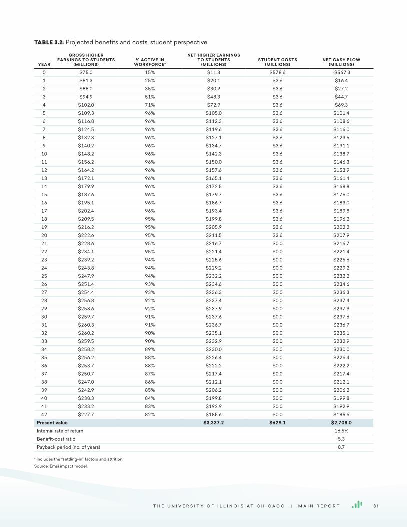
TABLE 3.2: Projected benefits and costs, student perspective

YEAR

GROSS HIGHER EARNINGS TO STUDENTS

(MILLIONS)% ACTIVE IN

WORKFORCE*

NET HIGHER EARNINGS TO STUDENTS

(MILLIONS)STUDENT COSTS

(MILLIONS)NET CASH FLOW

(MILLIONS)

0 $75.0 15% $11.3 $578.6 -$567.3

1 $81.3 25% $20.1 $3.6 $16.4

2 $88.0 35% $30.9 $3.6 $27.2

3 $94.9 51% $48.3 $3.6 $44.7

4 $102.0 71% $72.9 $3.6 $69.3

5 $109.3 96% $105.0 $3.6 $101.4

6 $116.8 96% $112.3 $3.6 $108.6

7 $124.5 96% $119.6 $3.6 $116.0

8 $132.3 96% $127.1 $3.6 $123.5

9 $140.2 96% $134.7 $3.6 $131.1

10 $148.2 96% $142.3 $3.6 $138.7

11 $156.2 96% $150.0 $3.6 $146.3

12 $164.2 96% $157.6 $3.6 $153.9

13 $172.1 96% $165.1 $3.6 $161.4

14 $179.9 96% $172.5 $3.6 $168.8

15 $187.6 96% $179.7 $3.6 $176.0

16 $195.1 96% $186.7 $3.6 $183.0

17 $202.4 96% $193.4 $3.6 $189.8

18 $209.5 95% $199.8 $3.6 $196.2

19 $216.2 95% $205.9 $3.6 $202.2

20 $222.6 95% $211.5 $3.6 $207.9

21 $228.6 95% $216.7 $0.0 $216.7

22 $234.1 95% $221.4 $0.0 $221.4

23 $239.2 94% $225.6 $0.0 $225.6

24 $243.8 94% $229.2 $0.0 $229.2

25 $247.9 94% $232.2 $0.0 $232.2

26 $251.4 93% $234.6 $0.0 $234.6

27 $254.4 93% $236.3 $0.0 $236.3

28 $256.8 92% $237.4 $0.0 $237.4

29 $258.6 92% $237.9 $0.0 $237.9

30 $259.7 91% $237.6 $0.0 $237.6

31 $260.3 91% $236.7 $0.0 $236.7

32 $260.2 90% $235.1 $0.0 $235.1

33 $259.5 90% $232.9 $0.0 $232.9

34 $258.2 89% $230.0 $0.0 $230.0

35 $256.2 88% $226.4 $0.0 $226.4

36 $253.7 88% $222.2 $0.0 $222.2

37 $250.7 87% $217.4 $0.0 $217.4

38 $247.0 86% $212.1 $0.0 $212.1

39 $242.9 85% $206.2 $0.0 $206.2

40 $238.3 84% $199.8 $0.0 $199.8

41 $233.2 83% $192.9 $0.0 $192.9

42 $227.7 82% $185.6 $0.0 $185.6

Present value $3,337.2 $629.1 $2,708.0Internal rate of return 16.5%

Benefit-cost ratio 5.3

Payback period (no. of years) 8.7

* Includes the “settling-in” factors and attrition.



discount rate is based upon student loan interest rates.34 In Chapter 4, we conduct a sensitivity analysis of this discount rate. The present value of the benefits is then compared to student costs to derive the investment analysis results, expressed in terms of a benefit-cost ratio, rate of return, and payback period. The investment is feasible if returns match or exceed the minimum threshold values; i.e., a benefit-cost ratio greater than 1, a rate of return that exceeds the discount rate, and a reasonably short payback period.

In Table 3.2, the net higher earnings of students yield a cumulative discounted sum of approximately $3.3 billion, the present value of all of the future earnings increments (see the bottom section of Column 4). This may also be interpreted as the gross capital asset value of the students’ higher earnings stream. In effect, the aggregate FY 2017 student body is rewarded for its investment in UIC with a capital asset valued at $3.3 billion.

The students’ cost of attending the university is shown in Column 5 of Table 3.2, equal to a present value of $629.1

34 The student discount rate is derived from the baseline forecasts for the 10-year Treasury rate published by the Congressional Budget Office. See the Congressional Budget Office, “Table 4. Projection of Borrower Interest Rates: CBO’s January 2017 Baseline”, Congressional Budget Office Publications, CBO’s January 2017 Baseline Projections for the Student Loan Program, last modified January 25, 2017, accessed Febru-ary 2017, https://www.cbo.gov/sites/default/files/recurringdata/51310-2017-01-studentloan.pdf.

million. Comparing the cost with the present value of ben-efits yields a student benefit-cost ratio of 5.3 (equal to $3.3 billion in benefits divided by $629.1 million in costs).

Another way to compare the same benefits stream and associated cost is to compute the rate of return. The rate of return indicates the interest rate that a bank would have to pay a depositor to yield an equally attractive stream of future payments.35 Table 3.2 shows students of UIC earning average returns of 16.5% on their investment of time and money. This is a favorable return compared, for example, to approximately 1% on a standard bank savings account, or 10% on stocks and bonds (30-year average return).

Note that returns reported in this study are real returns, not nominal. When a bank promises to pay a certain rate of interest on a savings account, it employs an implicitly nominal rate. Bonds operate in a similar manner. If it turns out that the inflation rate is higher than the stated rate of return, then money is lost in real terms. In contrast, a real rate of return is on top of inflation. For example, if inflation is running at 3% and a nominal percentage of 5% is paid, then the real rate of return on the investment is only 2%. In Table 3.2, the 16.5% student rate of return is a real rate. With an inflation rate of 2.1% (the average rate reported over the past 20 years as per the U.S. Department of Commerce, Consumer Price Index), the corresponding nominal rate of return is 18.7%, higher than what is reported in Table 3.2.

The payback period is defined as the length of time it takes to entirely recoup the initial investment.36 Beyond that point, returns are what economists would call pure costless rent. As indicated in Table 3.2, students at UIC see, on average,

35 Rates of return are computed using the familiar internal rate-of-return calculation. Note that, with a bank deposit or stock market investment, the depositor puts up a principal, receives in return a stream of periodic payments, and then recovers the principal at the end. Someone who invests in education, on the other hand, receives a stream of periodic payments that include the recovery of the principal as part of the periodic payments, but there is no principal recovery at the end. These differences notwithstanding comparable cash flows for both bank and education investors yield the same internal rate of return.

36 Payback analysis is generally used by the business community to rank alternative investments when safety of investments is an issue. Its great-est drawback is it does not take into account the time value of money. The payback period is calculated by dividing the cost of the investment by the net return per period. In this study, the cost of the investment includes tuition and fees plus the opportunity cost of time; it does not take into account student living expenses.

DISCOUNT RATE

The discount rate is a rate of interest that converts future costs and benefits to present values. For example, $1,000 in higher earnings realized 30 years in the future is worth much less than $1,000 in the present. All future values must therefore be expressed in present value terms in order to compare them with investments (i.e., costs) made today. The selection of an appropriate discount rate, however, can become an arbitrary and controversial undertaking. As suggested in economic theory, the discount rate should reflect the investor’s opportunity cost of capital, i.e., the rate of return one could reasonably expect to obtain from alternative investment schemes. In this study we assume a 4.5% discount rate from the student perspective and a 1.4% discount rate from the perspective of taxpayers and society.


a payback period of 8.7 years on their foregone earnings and out-of-pocket costs.

TAXPAYER PERSPECTIVE

In FY 2017, taxpayers invested in the University of Illinois System. In return for their investment, taxpayers will receive benefits from each of the University of Illinois universities. From the taxpayer perspective, the pivotal step here is to hone in on the public benefits that specifically accrue to state and local government from activities at UIC. For example, benefits resulting from earnings growth are limited to increased state and local tax payments. Similarly, savings related to improved health, reduced crime, and fewer wel-fare and unemployment claims, discussed below, are limited to those received strictly by state and local government. In all instances, benefits to private residents, local businesses, or the federal government are excluded.

Growth in state tax revenues

As a result of their time at UIC, students earn more because of the skills they learned while attending the university, and businesses earn more because student skills make capital more productive (buildings, machinery, and every-thing else). This in turn raises profits and other business property income. Together, increases in labor and non-labor (i.e., capital) income are considered the effect of a skilled workforce. These in turn increase tax revenues since state and local government is able to apply tax rates to higher earnings.

Estimating the effect of UIC on increased tax revenues begins with the present value of the students’ future earn-ings stream, which is displayed in Column 4 of Table 3.2. To this we apply a multiplier derived from Emsi’s MR-SAM model to estimate the added labor income created in the state as students and businesses spend their higher earnings.37 As labor income increases, so does non-labor income, which consists of monies gained through invest-ments. To calculate the growth in non-labor income, we multiply the increase in labor income by a ratio of the Illinois gross state product to total labor income in the state. We

37 For a full description of the Emsi MR-SAM model, see Appendix 4.

also include the spending impacts discussed in Chapter 2 that were created in FY 2017 from operations spending, research spending, student spending, and visitor spending. To each of these, we apply the prevailing tax rates so we capture only the tax revenues attributable to state and local government from this additional revenue.

Not all of these tax revenues may be counted as benefits to the state, however. Some students leave the state during the course of their careers, and the higher earnings they receive as a result of their education leaves the state with them. To account for this dynamic, we combine student settlement data from the university with data on migration patterns from the Census Bureau to estimate the number of students who will leave the state workforce over time.

We apply another reduction factor to account for the stu-dents’ alternative education opportunities. This is the same adjustment that we use in the calculation of the alumni impact in Chapter 2 and is designed to account for the counterfactual scenario where UIC does not exist. The assumption in this case is that any benefits generated by students who could have received an education even without the university cannot be counted as new benefits to society. For this analysis, we assume an alternative education variable of 15%, meaning that 15% of the student population at the university would have generated benefits anyway even without the university. For more information on the alternative education variable, see Appendix 6.

After adjusting for attrition and alternative education oppor-tunities, we calculate the present value of the future added tax revenues that occur in the state, equal to $1.2 billion. Recall from the discussion of the student return on invest-ment that the present value represents the sum of the future benefits that accrue each year over the course of the time horizon, discounted to current year dollars to account for the time value of money. Given that the stakeholder in this case is the public sector, we use the discount rate of 0.6%. This is the real treasury interest rate recommended by the Office of Management and Budget (OMB) for 30-year investments, and in Chapter 4, we conduct a sensitivity analysis of this discount rate.38

38 Office of Management and Budget. “Circular A-94 Appendix C.” Real Interest Rates on Treasury Notes and Bonds of Specified Maturities (in Percent). Last modified November 2016. Accessed January 2017. https://


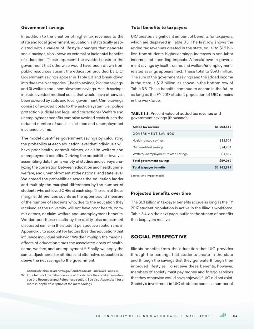
Government savings

In addition to the creation of higher tax revenues to the state and local government, education is statistically asso-ciated with a variety of lifestyle changes that generate social savings, also known as external or incidental benefits of education. These represent the avoided costs to the government that otherwise would have been drawn from public resources absent the education provided by UIC. Government savings appear in Table 3.3 and break down into three main categories: 1) health savings, 2) crime savings, and 3) welfare and unemployment savings. Health savings include avoided medical costs that would have otherwise been covered by state and local government. Crime savings consist of avoided costs to the justice system (i.e., police protection, judicial and legal, and corrections). Welfare and unemployment benefits comprise avoided costs due to the reduced number of social assistance and unemployment insurance claims.

The model quantifies government savings by calculating the probability at each education level that individuals will have poor health, commit crimes, or claim welfare and unemployment benefits. Deriving the probabilities involves assembling data from a variety of studies and surveys ana-lyzing the correlation between education and health, crime, welfare, and unemployment at the national and state level. We spread the probabilities across the education ladder and multiply the marginal differences by the number of students who achieved CHEs at each step. The sum of these marginal differences counts as the upper bound measure of the number of students who, due to the education they received at the university, will not have poor health, com-mit crimes, or claim welfare and unemployment benefits. We dampen these results by the ability bias adjustment discussed earlier in the student perspective section and in Appendix 5 to account for factors (besides education) that influence individual behavior. We then multiply the marginal effects of education times the associated costs of health, crime, welfare, and unemployment.39 Finally, we apply the same adjustments for attrition and alternative education to derive the net savings to the government.

obamawhitehouse.archives.gov/ omb/circulars_a094/a94_appx-c.39 For a full list of the data sources used to calculate the social externalities,

see the Resources and References section. See also Appendix 4 for a more in-depth description of the methodology.

Total benefits to taxpayers

UIC creates a significant amount of benefits for taxpayers, which are displayed in Table 3.3. The first row shows the added tax revenues created in the state, equal to $1.2 bil-lion, from students’ higher earnings, increases in non-labor income, and spending impacts. A breakdown in govern-ment savings by health, crime, and welfare/unemployment-related savings appears next. These total to $59.1 million. The sum of the government savings and the added income in the state is $1.3 billion, as shown in the bottom row of Table 3.3. These benefits continue to accrue in the future as long as the FY 2017 student population of UIC remains in the workforce.

Projected benefits over time

The $1.3 billion in taxpayer benefits accrue as long as the FY 2017 student population is active in the Illinois workforce. Table 3.4, on the next page, outlines the stream of benefits that taxpayers receive.

SOCIAL PERSPECTIVE

Illinois benefits from the education that UIC provides through the earnings that students create in the state and through the savings that they generate through their improved lifestyles. To receive these benefits, however, members of society must pay money and forego services that they otherwise would have enjoyed if UIC did not exist. Society’s investment in UIC stretches across a number of

TABLE 3.3: Present value of added tax revenue and government savings (thousands)

Added tax revenue $1,203,517

G OV E R N M E N T SAV I N G S

Health-related savings $32,509

Crime-related savings $24,701

Welfare/unemployment-related savings $1,852

Total government savings $59,062

Total taxpayer benefits $1,262,579



investor groups, from students to employers to taxpayers. We weigh the benefits generated by UIC to these investor groups against the total social costs of generating those benefits. The total social costs include all UIC expenditures, all student expenditures (including interest on student loans) less tuition and fees, and all student opportunity costs, totaling a present value of $2.3 billion.

On the benefits side, any benefits that accrue to Illinois as a whole – including students, employers, taxpayers, and anyone else who stands to benefit from the activities of UIC – are counted as benefits under the social perspec-tive. We group these benefits under the following broad headings: 1) increased earnings in the state, and 2) social externalities stemming from improved health, reduced crime, and reduced unemployment in the state (see the Beekeeper Analogy box for a discussion of externalities). Both of these benefits components are described more fully in the following sections.

BEEKEEPER ANALOGY

Beekeepers provide a classic example of positive exter-nalities (sometimes called “neighborhood effects”). The beekeeper’s intention is to make money selling honey. Like any other business, receipts must at least cover operating costs. If they don’t, the business shuts down.

But from society’s standpoint there is more. Flowers pro-vide the nectar that bees need for honey production, and smart beekeepers locate near flowering sources such as orchards. Nearby orchard owners, in turn, benefit as the bees spread the pollen necessary for orchard growth and fruit production. This is an uncompensated external ben-efit of beekeeping, and economists have long recognized that society might actually do well to subsidize positive externalities such as beekeeping.

Educational institutions are like beekeepers. While their principal aim is to provide education and raise people’s earnings, in the process an array of external benefits are created. Students’ health and lifestyles are improved, and society indirectly benefits just as orchard owners indi-rectly benefit from beekeepers. Aiming at a more complete accounting of the benefits generated by education, the model tracks and accounts for many of these external social benefits.

TABLE 3.4: Projected benefits, taxpayer perspective

YEARBENEFITS TO TAXPAYERS

(MILLIONS)

0 $186.3

1 $4.0

2 $6.1

3 $9.4

4 $14.1

5 $20.0

6 $21.0

7 $22.1

8 $23.2

9 $24.3

10 $25.3

11 $26.4

12 $27.4

13 $28.5

14 $29.5

15 $30.4

16 $31.3

17 $32.2

18 $33.0

19 $33.8

20 $34.5

21 $35.1

22 $35.6

23 $36.1

24 $36.5

25 $36.8

26 $37.0

27 $37.1

28 $37.2

29 $37.1

30 $36.9

31 $36.7

32 $36.3

33 $35.9

34 $35.3

35 $34.7

36 $34.0

37 $33.2

38 $32.3

39 $31.4

40 $30.4

41 $29.3

42 $28.1

Present value $1,262.6


Note that because the University of Illinois System receives the taxpayer funding and

controls the funding structure for the individual universities, measuring a benefit-cost

ratio and rate of return is not appropriate for the taxpayer perspective.


Growth in state economic base

In the process of absorbing the newly-acquired skills of students that attend UIC, not only does the productivity of the Illinois workforce increase, but so does the productivity of its physical capital and assorted infrastructure. Students earn more because of the skills they learned while attending the university, and businesses earn more because student skills make capital more productive (buildings, machinery, and everything else). This in turn raises profits and other business property income. Together, increases in labor and non-labor (i.e., capital) income are considered the effect of a skilled workforce.

Estimating the effect of UIC on the state’s economic base follows the same process used when calculating increased tax revenues in the taxpayer perspective. However, instead of looking at just the tax revenue portion, we include all of the added earnings and business output. We again factor in student attrition and alternative education opportunities.

After adjusting for attrition and alternative education oppor-tunities, we calculate the present value of the future added income that occurs in the state, equal to $13.2 billion. Recall from the discussion of the student and taxpayer perspec-tives that the present value represents the sum of the future benefits that accrue each year over the course of the time horizon, discounted to current year dollars to account for the time value of money. As stated in the taxpayer perspective, given that the stakeholder in this case is the public sector, we use the discount rate of 0.6%.

Social savings

Similar to the government savings discussed above, society as a whole sees savings due to external or incidental ben-efits of education. These represent the avoided costs that otherwise would have been drawn from private and public resources absent the education provided by UIC. Social benefits appear in Table 3.5 and break down into three main categories: 1) health savings, 2) crime savings, and 3) welfare and unemployment savings. These are similar to the categories from the taxpayer perspective above, although health savings now also include lost productivity and other effects associated with smoking, alcoholism, obesity, mental illness, and drug abuse. In addition to avoided costs to the justice system, crime savings also consist of avoided victim costs and benefits stemming from the added productivity

of individuals who otherwise would have been incarcerated. Welfare and unemployment benefits comprise avoided costs due to the reduced number of social assistance and unemployment insurance claims.

Table 3.5 displays the results of the analysis. The first row shows the increased economic base in the state, equal to $13.2 billion, from students’ higher earnings and their mul-tiplier effects, increases in non-labor income, and spend-ing impacts. Social savings appear next, beginning with a breakdown of savings related to health. These savings amount to a present value of $187.2 million, including sav-ings due to a reduced demand for medical treatment and social services, improved worker productivity and reduced absenteeism, and a reduced number of vehicle crashes and fires induced by alcohol or smoking-related incidents. Crime savings amount to $32.2 million, including savings

TABLE 3.5: Present value of the future increased economic base and social savings in the state (thousands)

Increased economic base $13,240,609

S O C I A L SAV I N G S

Health

Smoking $97,093

Alcoholism $26,448

Obesity $54,694

Mental illness $4,963

Drug abuse $3,985

Total health savings $187,183

Crime

Criminal justice system savings $23,938

Crime victim savings $1,549

Added productivity $6,726

Total crime savings $32,213

Welfare/unemployment

Welfare savings $684

Unemployment savings $1,168

Total welfare/unemployment savings $1,852

Total social savings $221,247

Total, increased economic base + social savings $13,461,857



associated with a reduced number of crime victims, added worker productivity, and reduced expenditures for police and law enforcement, courts and administration of justice, and corrective services. Finally, the present value of the savings related to welfare and unemployment amount to $1.9 million, stemming from a reduced number of per-sons in need of earnings assistance. All told, social savings amounted to $221.2 million in benefits to communities and citizens in Illinois.

The sum of the social savings and the increased state eco-nomic base is $13.5 billion, as shown in the bottom row of Table 3.5. These savings accrue in the future as long as the FY 2017 student population of UIC remains in the workforce.

Return on investment to society

Table 3.6, on the next page, presents the stream of benefits accruing to the Illinois society and the total social costs of generating those benefits. Comparing the present value of the benefits and the social costs, we have a benefit-cost ratio of 5.8. This means that for every dollar invested in an education from UIC, whether it is the money spent on day-to-day operations of the university or money spent by students on tuition and fees, an average of $5.80 in benefits will accrue to society in Illinois.40

With and without social savings

Earlier in this chapter, social savings attributable to educa-tion (reduced crime, lower welfare, lower unemployment, and improved health) were defined as externalities that are incidental to the operations of UIC. Some would ques-tion the legitimacy of including these social savings in the calculation of benefits to education, arguing that only the tangible benefits (higher earnings) should be counted. Table

40 The rate of return is not reported for the social perspective because the beneficiaries of the investment are not necessarily the same as the original investors.

3.4 and Table 3.6 are inclusive of social savings reported as attributable to UIC. Recognizing the other point of view, Table 3.7 shows the benefits for taxpayers and return on investment for the social perspective exclusive of social savings. As indicated, returns are still above threshold val-ues (a benefit-cost ratio greater than 1.0), confirming that society receives value from investing in UIC and taxpayers receive substantial benefits.

CONCLUSION

This chapter has shown that the education provided by UIC is an attractive investment to students with rates of return that exceed alternative investment opportunities. At the same time, the presence of the university expands the state economy and creates a wide range of positive social benefits that accrue to taxpayers and society in general within Illinois.

TABLE 3.7: Taxpayer and social perspectives with and without social savings

INCLUDING SOCIAL

SAVINGS

EXCLUDING SOCIAL

SAVINGS

TA X PAY E R P E R S P E C T I V E

Benefits, present value (thousands) $1,262,579 $1,203,517

S O C I A L P E R S P E C T I V E

Net present value (thousands) $13,461,857 $13,240,609

Benefit-cost ratio 5.8 5.7



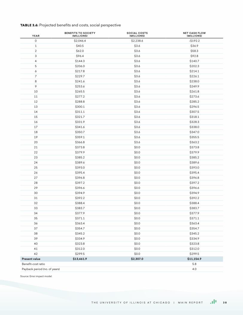
TABLE 3.6: Projected benefits and costs, social perspective

YEARBENEFITS TO SOCIETY

(MILLIONS)SOCIAL COSTS

(MILLIONS)NET CASH FLOW

(MILLIONS)

0 $2,046.4 $2,238.6 -$192.2

1 $40.5 $3.6 $36.9

2 $62.0 $3.6 $58.3

3 $96.4 $3.6 $92.8

4 $144.3 $3.6 $140.7

5 $206.0 $3.6 $202.3

6 $217.8 $3.6 $214.1

7 $229.7 $3.6 $226.1

8 $241.6 $3.6 $238.0

9 $253.6 $3.6 $249.9

10 $265.5 $3.6 $261.8

11 $277.2 $3.6 $273.6

12 $288.8 $3.6 $285.2

13 $300.1 $3.6 $296.5

14 $311.1 $3.6 $307.5

15 $321.7 $3.6 $318.1

16 $331.9 $3.6 $328.3

17 $341.6 $3.6 $338.0

18 $350.7 $3.6 $347.0

19 $359.1 $3.6 $355.5

20 $366.8 $3.6 $363.2

21 $373.8 $0.0 $373.8

22 $379.9 $0.0 $379.9

23 $385.2 $0.0 $385.2

24 $389.6 $0.0 $389.6

25 $393.0 $0.0 $393.0

26 $395.4 $0.0 $395.4

27 $396.8 $0.0 $396.8

28 $397.2 $0.0 $397.2

29 $396.6 $0.0 $396.6

30 $394.9 $0.0 $394.9

31 $392.2 $0.0 $392.2

32 $388.4 $0.0 $388.4

33 $383.7 $0.0 $383.7

34 $377.9 $0.0 $377.9

35 $371.1 $0.0 $371.1

36 $363.4 $0.0 $363.4

37 $354.7 $0.0 $354.7

38 $345.2 $0.0 $345.2

39 $334.9 $0.0 $334.9

40 $323.8 $0.0 $323.8

41 $312.0 $0.0 $312.0

42 $299.5 $0.0 $299.5

Present value $13,461.9 $2,307.0 $11,154.9


Payback period (no. of years) 4.0



C H A P T E R 4 :

Sensitivity Analysis

Sensitivity analysis measures the extent to which a model’s outputs are affected by hypo-

thetical changes in the background data and assumptions. This is especially important when

those variables are inherently uncertain. This analysis allows us to identify a plausible range

of potential results that would occur if the value of any of the variables is in fact different from

what was expected. In this chapter we test the sensitivity of the model to the following input

factors: 1) the alternative education variable, 2) the labor import effect variable, 3) the student

employment variables, 4) the discount rate, and 5) the retained student variable.

ALTERNATIVE EDUCATION VARIABLE

The alternative education variable (15%) accounts for the counterfactual scenario where students would have to seek a similar education elsewhere absent the publicly-funded university in the state. Given the difficulty in accurately specifying the alternative education variable, we test the sensitivity of the taxpayer and social analysis results to its magnitude. Variations in the alternative education assump-tion are calculated around base case results listed in the middle column of Table 4.1. Next, the model brackets the base case assumption on either side with a plus or minus 10%, 25%, and 50% variation in assumptions. Analyses are then repeated introducing one change at a time, holding all other variables constant. For example, an increase of

10% in the alternative education assumption (from 15% to 17%) reduces the taxpayer perspective benefits from $1.26 billion to $1.24 billion. Likewise, a decrease of 10% (from 15% to 14%) in the assumption increases the benefits from $1.26 billion to $1.28 billion.

Based on this sensitivity analysis, the conclusion can be drawn that UIC analysis results from the taxpayer and social perspectives are not very sensitive to relatively large varia-tions in the alternative education variable. As indicated, results are still above their threshold levels, even when the alternative education assumption is increased by as much as 50% (from 15% to 23%). The conclusion is that although the assumption is difficult to specify, its impact on overall results for the taxpayer and social perspectives is not very sensitive.

TABLE 4.1: Sensitivity analysis of alternative education variable, taxpayer and social perspectives

% VARIATION IN ASSUMPTION -50% -25% -10% BASE CASE 10% 25% 50%

Alternative education variable 8% 11% 14% 15% 17% 19% 23%


Benefits, present value (millions) $1,374 $1,318 $1,285 $1,263 $1,240 $1,207 $1,151


Net present value (millions) $12,343 $11,749 $11,392 $11,155 $10,917 $10,561 $9,967

Benefit-cost ratio 6.4 6.1 5.9 5.8 5.7 5.6 5.3


LABOR IMPORT EFFECT VARIABLE

The labor import effect variable only affects the alumni impact calculation in Table 2.14. In the model we assume a labor import effect variable of 50%, which means that 50% of the state’s labor demands would have been satisfied without the presence of UIC. In other words, businesses that hired UIC students could have substituted some of these workers with equally-qualified people from outside the state had there been no UIC students to hire. Therefore, we attribute only the remaining 50% of the initial labor income generated by increased alumni productivity to the university.

Table 4.2 presents the results of the sensitivity analysis for the labor import effect variable. As explained earlier, the assumption increases and decreases relative to the base case of 50% by the increments indicated in the table. Alumni productivity impacts attributable to UIC, for example, range from a high of $5.6 billion at a -50% variation to a low of $1.9 billion at a +50% variation from the base case assumption. This means that if the labor import effect variable increases, the impact that we claim as attributable to alumni decreases. Even under the most conservative assumptions, the alumni impact on the Illinois economy still remains sizeable.

STUDENT EMPLOYMENT VARIABLES

Student employment variables are difficult to estimate because many students do not report their employment status or because universities generally do not collect this kind of information. Employment variables include the fol-lowing: 1) the percentage of students that are employed while attending the university and 2) the percentage of earn-ings that working students receive relative to the earnings they would have received had they not chosen to attend the university. Both employment variables affect the investment analysis results from the student perspective.

Students incur substantial expense by attending UIC

because of the time they spend not gainfully employed. Some of that cost is recaptured if students remain partially (or fully) employed while attending. It is estimated that 75% of students are employed.41 This variable is tested in the sen-sitivity analysis by changing it first to 100% and then to 0%.

The second student employment variable is more difficult to estimate. In this study we estimate that students that are working while attending the university earn only 69%, on average, of the earnings that they statistically would have received if not attending UIC. This suggests that many students hold part-time jobs that accommodate their UIC attendance, though it is at an additional cost in terms of receiving a wage that is less than what they otherwise might make. The 69% variable is an estimation based on the average hourly wages of the most common jobs held by students while attending college relative to the aver-age hourly wages of all occupations in the U.S. The model captures this difference in wages and counts it as part of the opportunity cost of time. As above, the 69% estimate is tested in the sensitivity analysis by changing it to 100% and then to 0%.

The changes generate results summarized in Table 4.3, on the next page, with A defined as the percent of students employed and B defined as the percent that students earn relative to their full earning potential. Base case results appear in the shaded row; here the assumptions remain unchanged, with A equal to 75% and B equal to 69%. Sen-sitivity analysis results are shown in non-shaded rows. Scenario 1 increases A to 100% while holding B constant, Scenario 2 increases B to 100% while holding A constant, Scenario 3 increases both A and B to 100%, and Scenario 4 decreases both A and B to 0%.

• Scenario 1: Increasing the percentage of students employed (A) from 75% to 100%, the net present value,

41 Emsi provided an estimate of the percentage of students employed because UIC was unable to provide data.

TABLE 4.2: Sensitivity analysis of labor import effect variable


Labor import effect variable 25% 38% 45% 50% 55% 63% 75%

Alumni impact (millions) $5,643 $4,702 $4,138 $3,762 $3,386 $2,821 $1,881


internal rate of return, and benefit-cost ratio improve to $2.8 billion, 18.4%, and 6.2, respectively, relative to base case results. Improved results are attributable to a lower opportunity cost of time; all students are employed in this case.

• Scenario 2: Increasing earnings relative to statistical averages (B) from 69% to 100%, the net present value, internal rate of return, and benefit-cost ratio results improve to $2.8 billion, 19.6%, and 6.7, respectively, rela-tive to base case results; a strong improvement, again attributable to a lower opportunity cost of time.

• Scenario 3: Increasing both assumptions A and B to 100% simultaneously, the net present value, internal rate of return, and benefit-cost ratio improve yet further to $3 billion, 24.7%, and 9.2, respectively, relative to base case results. This scenario assumes that all students are fully employed and earning full salaries (equal to statistical averages) while attending classes.

• Scenario 4: Finally, decreasing both A and B to 0% reduces the net present value, internal rate of return, and benefit-cost ratio to $2.4 billion, 12.8%, and 3.7, respectively, relative to base case results. These results are reflective of an increased opportunity cost; none of the students are employed in this case.42

It is strongly emphasized in this section that base case results are very attractive in that results are all above their threshold levels. As is clearly demonstrated here, results of the first three alternative scenarios appear much more attractive, although they overstate benefits. Results pre-

42 Note that reducing the percent of students employed to 0% automati-cally negates the percent they earn relative to full earning potential, since none of the students receive any earnings in this case.

sented in Chapter 3 are realistic, indicating that investments in UIC generate excellent returns, well above the long-term average percent rates of return in stock and bond markets.

DISCOUNT RATE

The discount rate is a rate of interest that converts future monies to their present value. In investment analysis, the discount rate accounts for two fundamental principles: 1) the time value of money, and 2) the level of risk that an investor is willing to accept. Time value of money refers to the value of money after interest or inflation has accrued over a given length of time. An investor must be willing to forego the use of money in the present to receive compensation for it in the future. The discount rate also addresses the investors’ risk preferences by serving as a proxy for the minimum rate of return that the proposed risky asset must be expected to yield before the investors will be persuaded to invest in it. Typically, this minimum rate of return is determined by the known returns of less risky assets where the investors might alternatively consider placing their money.

In this study, we assume a 3.8% discount rate for students and a 0.6% discount rate for taxpayers and society.43 Similar to the sensitivity analysis of the alternative education vari-able, we vary the base case discount rates for students, taxpayers, and society on either side by increasing the discount rate by 10%, 25%, and 50%, and then reducing it

43 These values are based on the baseline forecasts for the 10-year Treasury rate published by the Congressional Budget Office and the real treasury interest rates recommended by the Office of Management and Budget for 30-year investments. See the Congressional Budget Office “Table 4. Projection of Borrower Interest Rates: CBO’s January 2017 Baseline” and the Office of Management and Budget “Circular A-94 Appendix C.”

TABLE 4.3: Sensitivity analysis of student employment variables

% VARIATION IN ASSUMPTION NET PRESENT VALUE (MILLIONS) INTERNAL RATE OF RETURN BENEFIT-COST RATIO

Base case: A = 75%, B = 69% $2,708.0 16.5% 5.3

Scenario 1: A = 100%, B = 69% $2,796.3 18.4% 6.2

Scenario 2: A = 75%, B = 100% $2,842.1 19.6% 6.7

Scenario 3: A = 100%, B = 100% $2,975.1 24.7% 9.2

Scenario 4: A = 0%, B = 0% $2,443.3 12.8% 3.7

Note: A = percent of students employed; B = percent earned relative to statistical averages


by 10%, 25%, and 50%. Note that, because the rate of return and the payback period are both based on the undiscounted cash flows, they are unaffected by changes in the discount rate. As such, only variations in the net present value and the benefit-cost ratio are shown for students and society in Table 4.4.

As demonstrated in the table, an increase in the discount rate leads to a corresponding decrease in the expected benefits and returns, and vice versa. For example, increas-ing the student discount rate by 50% (from 3.8% to 5.6%) reduces the students’ benefit-cost ratio from 5.3 to 4.5. Conversely, reducing the discount rate for students by 50% (from 3.8% to 1.9%) increases the benefit-cost ratio from 5.3 to 7.8. The sensitivity analysis results for society show the same inverse relationship between the discount rate and the benefit-cost ratio.

RETAINED STUDENT VARIABLE

The retained student variable only affects the student spending impact calculation in Table 2.9. For this analysis,

we assume a retained student variable of 15%, which means that 15% of UIC’s students who originated from Illinois would have left the state for other opportunities, whether that be education or employment, if UIC did not exist. The money these retained students spent in the state for accom-modation and other personal and household expenses is attributable to UIC.

Table 4.5 presents the results of the sensitivity analysis for the retained student variable. The assumption increases and decreases relative to the base case of 15% by the incre-ments indicated in the table. The student spending impact is recalculated at each value of the assumption, holding all else constant. Student spending impacts attributable to UIC range from a high of $106.5 million when the retained student variable is 23% to a low of $68 million when the retained student variable is 8%. This means as the retained student variable decreases, the student spending attribut-able to UIC decreases. Even under the most conservative assumptions, the student spending impact on the Illinois economy remains substantial.

TABLE 4.4: Sensitivity analysis of discount rate


S T U D E N T P E R S P E C T I V E

Discount rate 1.9% 2.8% 3.4% 3.8% 4.1% 4.7% 5.6%




Discount rate 0.3% 0.5% 0.5% 0.6% 0.7% 0.8% 0.9%

Benefits, present value (millions) $1,341 $1,301 $1,278 $1,263 $1,248 $1,226 $1,191


Discount rate 0.3% 0.5% 0.5% 0.6% 0.7% 0.8% 0.9%



TABLE 4.5: Sensitivity analysis of retained student variable


Retained student variable 8% 11% 14% 15% 17% 19% 23%

Student spending impact (thousands) $67,964 $77,602 $83,384 $87,239 $91,094 $96,877 $106,514


C H A P T E R 5 :

Conclusion

While UIC’s value to Illinois is larger than simply its economic impact, understanding the dol-

lars and cents value is an important asset to understanding the university’s value as a whole. In

order to fully assess UIC’s value to the state economy, this report has evaluated the university

from the perspectives of economic impact analysis and investment analysis.

From an economic impact perspective, we calculated that UIC generates a total economic impact of $7.6 billion in total added income for the state economy. This represents the sum of several different impacts, including the univer-sity’s operations spending impact ($1.5 billion), research spending impact ($424.6 million), hospital spending impact ($1.5 billion), impact from start-up companies ($342.7 mil-lion), student spending impact ($87.2 million), visitor spend-ing impact ($4 million), and alumni impact ($3.8 billion). This impact is equivalent to supporting 73,559 jobs in Illinois. For perspective, this means that one out of every 106 jobs in Illinois is supported by the activities of UIC and its students.

Since UIC’s activity represents an investment by various parties, including students and society as a whole, we also considered the university as an investment to see the value it provides to these investors. For each dollar invested by students and society, UIC offers a benefit of $5.30 and $5.80, respectively. State and local taxpayers will receive $1.3 billion in benefits throughout the students’ working lives.

Modeling the impact of the university is subject to many fac-tors, the variability of which we considered in our sensitivity analysis. With this variability accounted for, we present the findings of this study as a robust picture of the economic value of UIC.


Resources and References

Administration for Children and Families. “Characteristics and Financial Circumstances of TANF Recipients, Fiscal Year 2010.” August 2012. Accessed July 2013. http://www.acf.hhs.gov/sites/default/files/ofa/appen-dix_ys_final.pdf.

Administration for Children and Families. “Fiscal Year 2011 TANF Financial Data.” Office of Family Assistance, TANF Financial Data. August 2012. Accessed August 2013. http://www.acf.hhs.gov/programs/ofa/resource/tanf-financial-data-fy-2011.

American Automobile Association. “AAA Average Costs Per Mile.” Your Driving Costs AAA Association Commu-nication. 2012. Accessed May 2012. http://newsroom.aaa.com/wp-content/uploads/2012/04/YourDriving-Costs2012.pdf.

Arias, Elizabeth. “United States Life Tables, 2008.” National Vital Statistics Reports 61, no. 3 (September 24, 2012). Hyattsville, MD: National Center for Health Statistics. Accessed February 2017. http://www.cdc.gov/nchs/data/nvsr/nvsr61/nvsr61_03.pdf.

Baryla, Edward and Douglas Dotterweich. “Student Migra-tion: Do Significant Factors Vary by Region?” Educa-tion Economics 9, no. 3 (2001).

Becker, Gary S. Human Capital: A Theoretical and Empirical Analysis, with Special Reference to Education. New York: Columbia College Press for NBER, 1964.

Bilkic, Natasa, Thomas Gries, and Margarethe Pilichowski. “Stay in School or Start Working? The Human Capital Investment Decision under Uncertainty and Irrevers-ibility.” Labour Economics 19, no. 5 (October 2012): 706-717.

Bouchery, Ellen, Carol Simon, and Hendrick Harwood. “Economic Costs of Excessive Alcohol Consump-tion in the United States, 2006.” The Lewin Group. Report prepared for the Centers for Disease Control and Prevention and the National Foundation for the

Centers for Disease Control and Prevention. Febru-ary 2013. Accessed August 2013. http://www.lewin.com/~/media/Lewin/Site_Sections/Publications/CDC_Report_Rev.pdf.

Bureau of Economic Analysis. “Table 1.1.6. Real Gross Domes-tic Product, Chained Dollars.” GDP and Personal Income. Last modified January 27, 2017. Accessed February 2017. http://www.bea.gov/iTable/iTableHtml.cfm?reqid=9&step=3&isuri=1&903=6.

Bureau of Justice Statistics. “Appendix Table 1: Prisoners under the Jurisdiction of State or Federal Correc-tional Authorities, by Jurisdiction, December 31, 2000, 2008, and 2009.” Prisoners in 2009 (revised) NCJ 231675. Last modified October 2011. Accessed July 2013. http://www.bjs.gov/content/pub/pdf/p09.pdf.

Bureau of Labor Statistics. “Charts by Topic: Leisure and Sports Activities.” American Time Use Survey. December 2016. Accessed January 2017. http://www.bls.gov/TUS/CHARTS/LEISURE.HTM.

Bureau of Labor Statistics. “Charts by Topic: Students.” American Time Use Survey. December 2016. Accessed January 2017. https://www.bls.gov/TUS/CHARTS/STUDENTS.HTM.

Bureau of Labor Statistics. “Earnings and Unemployment Rates by Educational Attainment, 2015.” BLS Employ-ment Projections. March 2016. Accessed January 2017. https://www.bls.gov/emp/ep_chart_001.htm.

Bureau of Labor Statistics. “Table A-10. Unemployment Rates by Age, Sex, and Marital Status, Seasonally Adjusted.” Labor Force Statistics from the Current Population Survey. Last modified February 3, 2017. Accessed February 2017. https://www.bls.gov/web/empsit/cpseea10.htm.

Bureau of Labor Statistics. “Table 3.3: Civilian Labor Force Participation Rate by Age, Gender, Race and Eth-nicity, 1994, 2004, 2014, and Projected 2024 (In Per-


http://www.acf.hhs.gov/sites/default/files/ofa/appendix_ys_final.pdf

http://www.acf.hhs.gov/sites/default/files/ofa/appendix_ys_final.pdf

http://www.acf.hhs.gov/programs/ofa/resource/tanf-financial-data-fy-2011

http://www.acf.hhs.gov/programs/ofa/resource/tanf-financial-data-fy-2011

http://newsroom.aaa.com/wp-content/uploads/2012/04/YourDrivingCosts2012.pdf



http://www.cdc.gov/nchs/data/nvsr/nvsr61/nvsr61_03.pdf

http://www.cdc.gov/nchs/data/nvsr/nvsr61/nvsr61_03.pdf

http://www.lewin.com/~/media/Lewin/Site_Sections/Publications/CDC_Report_Rev.pdf



http://www.bea.gov/iTable/iTableHtml.cfm?reqid=9&step=3&isuri=1&903=6

http://www.bea.gov/iTable/iTableHtml.cfm?reqid=9&step=3&isuri=1&903=6

http://www.bjs.gov/content/pub/pdf/p09.pdf

http://www.bls.gov/TUS/CHARTS/LEISURE.HTM

http://www.bls.gov/TUS/CHARTS/LEISURE.HTM

https://www.bls.gov/TUS/CHARTS/STUDENTS.HTM

https://www.bls.gov/TUS/CHARTS/STUDENTS.HTM

https://www.bls.gov/emp/ep_chart_001.htm

https://www.bls.gov/web/empsit/cpseea10.htm

https://www.bls.gov/web/empsit/cpseea10.htm

cent).” Employment Projections. December 2016. Accessed February 2017. https://www.bls.gov/emp/ep_table_303.htm.

Bureau of Labor Statistics. “Table 24: Historical Consumer Price Index for all Urban Consumers (CPI-U): U.S. City Average, All Items.” CPI Detailed Report: Data for December 2015. December 2015. Accessed January 2017. https://www.bls.gov/cpi/cpid1512.pdf.

Buss, Christian, Jeffrey Parker, and Jon Rivenburg. “Cost, Quality and Enrollment Demand at Liberal Arts Col-leges.” Economics of Education Review 23, no. 1 (Feb-ruary 2004): 57-65.

Card, David. “The Causal Effect of Education on Earnings.” Handbook of Labor Economics 3 (1999): 1801-1863.

Card, David. “Estimating the Return to Schooling: Progress on Some Persistent Econometric Problems.” Econo-metrica 69, no. 5 (September 2001): 1127-1160.

Carson, Ann E. and Daniela Golinelli. “Table 1: Prisoners Under the Jurisdiction of State or Federal Correc-tional Authorities, December 31, 2002–2012.” Bureau of Justice Statistics: Prisoners in 2012 - Advance Counts NCJ 242467 (July 2013). Accessed August 2013. http://www.bjs.gov/content/pub/pdf/p12ac.pdf.

Center on Budget and Policy Priorities. “Policy Basics - How Many Weeks of Unemployment are Available?” Last modified August 26, 2013. Accessed August 27, 2013. http://www.cbpp.org/files/PolicyBasics_UI_Weeks.pdf.

Centers for Disease Control and Prevention. “Adult Obe-sity Facts.” Overweight and Obesity. Accessed August 2013. http://www.cdc.gov/obesity/data/adult.html#Prevalence.

Centers for Disease Control and Prevention. “Current Cigarette Use Among Adults (Behavior Risk Factor Surveillance System) 2016.” Behavioral Risk Factor Surveillance System Prevalence and Trends Data [Data set]. Accessed March 2018. https://www.cdc.gov/statesystem/cigaretteuseadult.html.

Centers for Disease Control and Prevention. “Heavy Drinkers (Adult Men Having More Than Two Drinks per Day and Adult Women Having More Than One Drink per

Day).” Alcohol Consumption - 2012 Behavioral Risk Factor Surveillance System Prevalence and Trends Data. Accessed August 2013. http://apps.nccd.cdc.gov/brfss/list.asp?cat=AC&yr=2012&qkey=8381&state=All.

Centers for Disease Control and Prevention. “Table 1. Num-ber of Respondents to a Question about Mental Health and Percentage who Self-Reported Frequent Mental Distress (FMD), by Demographic Character-istics – United States, Behavioral Risk Factor Surveil-lance System, 1993-1996.” Self-Reported Frequent Mental Distress Among Adults – United States, 1993-1996 Morbidity and Mortality Weekly Report 47, no. 16 (May 1998): 325-331.

Centers for Disease Control and Prevention. “Table 3: Preva-lence of Current Depression among Adults Aged ≥18 Years, by Sociodemographic Characteristics and Year – Behavioral Risk Factor Surveillance System, Mul-tiple States, 2006 and 2008.” Mental Illness Surveil-lance Among Adults in the United States Morbidity and Mortality Weekly Report 60 (September 2011): 17.

Centers for Disease Control and Prevention. “Table. Char-acteristics of Current Adult Cigarette Smokers.” National Health Interview Survey, United States, 2016. Accessed March 2018. https://www.cdc.gov/mmwr/volumes/67/wr/mm6702a1.htm#T1_down.

Centers for Medicare and Medicaid Services. “Table 16: National Health Expenditures, Amounts and Aver-age Annual Growth from Previous Year Shown, by Type of Sponsor, Selected Calendar Years 2009-2025.” NHE Projections 2015-2025 – Tables. February 2016. Accessed January 2017. https://www.cms.gov/Research-Statistics-Data-and-Systems/Statistics-Trends-and-Reports/NationalHealthExpendData/NationalHealthAccountsProjected.html.

College Board. “Figure 1: Average Estimated Full-Time Undergraduate Budgets, 2012-13 (Enrollment-Weighted).” The College Board, Annual Survey of Colleges, Average Estimated Undergraduate Bud-gets, 2012-13. Accessed August 2013. http://trends.collegeboard.org/college-pricing/figures-tables/average-estimated-undergraduate-budgets-2012-13.

Congressional Budget Office. “Table 4. Projection of Bor-


https://www.bls.gov/emp/ep_table_303.htm

https://www.bls.gov/emp/ep_table_303.htm

https://www.bls.gov/cpi/cpid1512.pdf

http://www.bjs.gov/content/pub/pdf/p12ac.pdf

http://www.cbpp.org/files/PolicyBasics_UI_Weeks.pdf

http://www.cbpp.org/files/PolicyBasics_UI_Weeks.pdf

https://www.cdc.gov/statesystem/cigaretteuseadult.html

https://www.cdc.gov/statesystem/cigaretteuseadult.html

http://apps.nccd.cdc.gov/brfss/list.asp?cat=AC&yr=2012&qkey=8381&state=All



https://www.cms.gov/Research-Statistics-Data-and-Systems/Statistics-Trends-and-Reports/NationalHealthExpendData/NationalHealthAccountsProjected.html




http://trends.collegeboard.org/college-pricing/figures-tables/average-estimated-undergraduate-budgets-2012-13



rower Interest Rates: CBO’s June 2017 Baseline.” Congressional Budget Office Publications CBO’s June 2017 Baseline Projections for the Student Loan Program. Last modified June 2017. Accessed March 2018. https://www.cbo.gov/sites/default/files/recurringdata/51310-2017-06-studentloan.pdf.

Criminal Justice Expenditure and Employment Extracts Program. “Table 4. Justice System Expenditure by Character, State and Type of Government, Fiscal Year 2009 (Preliminary).” Justice Expenditure and Employment Extracts 2009 (preliminary) NCJ 237913. Accessed July 2013. http://bjs.ojp.usdoj.gov/index.cfm?ty=pbdetail&iid=4335.

Dickerson, Andy, and Steven McIntosh. “The Impact of Distance to Nearest Education Institution on the Post Compulsory Education Participation Decision.” Urban Studies 50, no. 4 (2013): 742-758.

Dynarski, Susan M. “Does Aid Matter? Measuring the Effect of Student Aid on College Attendance and Comple-tion.” American Economic Review 93, no. 1 (2003): 279-288.

Emsi Labor Market Data and Software. www.economic-modeling.com.

Federal Bureau of Investigation, Criminal Justice Information Services Division. “Table 12: Crime Trends by Popu-lation Group, 2009-2010.” Uniform Crime Reports, Crime in the United States, Offenses Known to Law Enforcement. Accessed August 2013. http://www.fbi.gov/about-us/cjis/ucr/crime-in-the-u.s/2010/crime-in-the-u.s.-2010/offenses-known-to-law-enforcement.

Federal Bureau of Investigation, Criminal Justice Infor-mation Services Division. “Table 29: Estimated Number of Arrests, United States, 2010.” Uniform Crime Reports, Crime in the United States, Persons Arrested. Accessed August 2013. http://www.fbi.gov/about-us/cjis/ucr/crime-in-the-u.s/2010/crime-in-the-u.s.-2010/tables/10tbl29.xls.

Federal Bureau of Prisons. “Quick Facts About the Bureau of Prisons.” Last modified July 27, 2013. Accessed August 19, 2013. http://www.bop.gov/news/quick.jsp#1.

Finkelstein, Eric A., Marco da Costa DiBonaventura, Somali M. Burgess, and Brent C. Hale. “The Costs of Obe-sity in the Workplace.” Journal of Occupational and Environmental Medicine 52, no. 10 (October 2010): 971-976.

Guerino, Paul, Paige M. Harrison, and William J. Sabol. “Prisoners in 2010.” Bureau of Justice Statistics NCJ 236096 (December 2011). Accessed August 2013. http://www.bjs.gov/content/pub/pdf/p10.pdf.

Hamadeh, Mohamad and Roy Khoueiri. “Demand Elasticities for Higher Education in the United States.” Interna-tional Journal of Business and Economic Perspec-tives 5, no. 2 (2010): 60-67.

Harlow, Caroline Wolf. “Table 1. Educational Attainment for State and Federal Prison Inmates, 1997 and 1991, Local Jail Inmates, 1996 and 1989, Probationers, 1995, and the General Population, 1997.” Education and Correctional Populations, Bureau of Justice Sta-tistics Special Report NCJ 195670 (January 2003). Accessed August 2013. http://bjs.ojp.usdoj.gov/index.cfm?ty=pbdetail&iid=814.

Henderson, James M. and Richard E. Quandt. Microeco-nomic Theory: A Mathematical Approach. New York: McGraw-Hill Book Company, 1971.

Hernández-Murillo, Rubén, Lesli S. Ott, Michael T. Owyang, and Denise Whalen. “Patterns of Interstate Migra-tion in the United States from the Survey of Income and Program Participation.” Federal Reserve Bank of St. Louis Review 93, no. 3 (May/June 2011): 169-186. Accessed February 2017. https://files.stlouisfed.org/files/htdocs/publications/review/11/05/169-186Her-nandez.pdf.

IHS Consulting. “North Carolina Tourism 2011.” Accessed March 27, 2013. http://www.travelks.com/includes/content/docs/media/2011-North Carolina-TSA-Results-with-Regional-Analysis.pdf.

Jaeger, David A. and Marianne E. Page. “New Evidence on Sheepskin Effects in the Returns to Education.” The Review of Economics and Statistics 78, no. 4 (November 1996): 733-740.

Jamal Ahmed, Elyse Phillips, Andrea S. Gentzke, David M.


https://www.cbo.gov/sites/default/files/recurringdata/51310-2017-06-studentloan.pdf

https://www.cbo.gov/sites/default/files/recurringdata/51310-2017-06-studentloan.pdf

http://bjs.ojp.usdoj.gov/index.cfm?ty=pbdetail&iid=4335


http://www.economicmodeling.com

http://www.economicmodeling.com

http://www.fbi.gov/about-us/cjis/ucr/crime-in-the-u.s/2010/crime-in-the-u.s.-2010/offenses-known-to-law-enforcement




http://www.fbi.gov/about-us/cjis/ucr/crime-in-the-u.s/2010/crime-in-the-u.s.-2010/tables/10tbl29.xls



http://www.bjs.gov/content/pub/pdf/p10.pdf



https://files.stlouisfed.org/files/htdocs/publications/review/11/05/169-186Hernandez.pdf



http://www.travelks.com/includes/content/docs/media/2011-North%20Carolina-TSA-Results-with-Regional-Analysis.pdf



Homa, Stephen D. Babb, Brian A. King, and Linda J. Neff. “Current Cigarette Smoking Among Adults – United States, 2016.” Morbidity and Mortality Weekly Report 2018 67:53-59. DOI: http://dx.doi.org/10.15585/mmwr.mm6702a1.

Kaeding, Nicole. “State Individual Income Tax Rates and Brackets for 2016.” Tax Foundation Fiscal Fact no. 500 (February 2016). Accessed January 2017. https://files.taxfoundation.org/legacy/docs/TaxFoundation_FF500.pdf.

Kelchtermans, Stijn and Frank Verboven. “Participation and Study Decisions in a Public System of Higher Edu-cation.” Journal of Applied Econometrics 25, no. 3 (2010): 355-391.

Leigh, Andrew and Chris Ryan. “Estimating Returns to Edu-cation Using Different Natural Experiments Tech-niques.” Economics of Education Review 27 (2008): 149-160.

Leonesio, Michael V. “The Economics of Retirement: A Nontechnical Guide.” Social Security Bulletin 59, no. 4 (Winter 1996): 29-50.

McCollister, Kathryn E., Michael T. French, and Hai Fang. “The Cost of Crime to Society: New Crime-Specific Estimates for Policy and Program Evaluation.” Drug and Alcohol Dependence 108, no. 1-2 (April 1, 2010): 98-109. Accessed August 2013. http://www.ncbi.nlm.nih.gov/pmc/articles/PMC2835847.

Mincer, Jacob. “Investment in Human Capital and Personal Income Distribution.” Journal of Political Economy 66, no. 4 (August 1958): 281–302.

Mincer, Jacob. Schooling, Experience and Earnings. New York: National Bureau of Economic Research, 1974.

Minton, Todd. “Table 1: Inmates Confined in Local Jails at Midyear, Average Daily Population, and Incarceration Rates, 2000–2012.” Jail Inmates at Midyear 2012 - Statistical Tables Bureau of Justice Statistics NCJ 241264 (May 2013). Accessed August 2013. www.bjs.gov/content/pub/pdf/jim12st.pdf.

Morgan, James N. and Edward H. Robb. “The Impact of Age Upon Interregional Migration.” The Annals of Regional Science 15, no. 3 (November 1981): 31-45.

National Center for Education Statistics. Integrated Post-secondary Education Data System (IPEDS). http://nces.ed.gov/ipeds.

National Center for Education Statistics. “Table 219.60 Number of People Taking the GED Test and Per-centage Distribution of Those who Passed, by Age Group: 1971 through 2013.” Digest of Education Sta-tistics. 2015. Accessed January 2017. https://nces.ed.gov/programs/digest/d15/tables/dt15_219.60.asp?current=yes.

National Center for Education Statistics. “Table 507.20 Par-ticipants in State-Administered Adult Basic Educa-tion, Secondary Education, and English as a Second Language Programs, by Type of Program and State or Jurisdiction: Selected Fiscal Years, 2000 through 2014.” Digest of Education Statistics. 2015. Accessed January 2017. https://nces.ed.gov/programs/digest/d15/tables/dt15_507.20.asp?current=yes.

National Center for Health Statistics. “Table 74. Healthy Weight, Overweight, and Obesity Among Persons 20 Years of Age and Over, by Selected Characteristics: United States, Selected Years 1960-1962 through 2007-2010.” Centers for Disease Control and Pre-vention, Health, United States, 2011. Last modified March 14, 2013. Accessed August 2013. https://www.cdc.gov/nchs/data/hus/2011/074.pdf.

National Survey on Drug Use and Health. “Table B.1 – Illicit Drug Use in the Past Month, by Age Group and State: Percentages, Annual Averages Based on 2009 and 2010 NSDUHs.” State Estimates of Substance Use and Mental Disorders from the 2009-2010 National Surveys on Drug Use and Health. Substance Abuse and Mental Health Services Administration no. 12-4703 (2012).

National Survey on Drug Use and Health. “Table 1 (Revised). Serious Mental Illness (SMI) in Past Year among Per-sons Aged 18 or Older, by Location: Percentages, Annual Averages Based on 2008 and 2009 NSDUHs.” The NSDUH Mental Illness: State Estimates of Adult Mental Illness. Center for Behavioral Health Statistics and Quality, Substance Abuse and Mental Health Services Administration (May 2012).

OECD. “Household Net Saving Rates: As a Percentage of


http://dx.doi.org/10.15585/mmwr.mm6702a1

http://dx.doi.org/10.15585/mmwr.mm6702a1

https://files.taxfoundation.org/legacy/docs/TaxFoundation_FF500.pdf



http://www.ncbi.nlm.nih.gov/pmc/articles/PMC2835847/

http://www.ncbi.nlm.nih.gov/pmc/articles/PMC2835847/

http://www.bjs.gov/content/pub/pdf/jim12st.pdf

http://www.bjs.gov/content/pub/pdf/jim12st.pdf

http://nces.ed.gov/ipeds/

http://nces.ed.gov/ipeds/

https://nces.ed.gov/programs/digest/d15/tables/dt15_219.60.asp?current=yes





https://www.cdc.gov/nchs/data/hus/2011/074.pdf

https://www.cdc.gov/nchs/data/hus/2011/074.pdf

Household Disposable Income.” OECD Factbook 2015-2016: Economic, Environmental and Social Sta-tistics (2016). Accessed January 2017. http://dx.doi.org/10.1787/factbook-2015-19-en.

Office of Management and Budget. “Circular A-94 Appendix C.” Real Interest Rates on Treasury Notes and Bonds of Specified Maturities (in Percent). Last modified November 2017. Accessed January 2018. https://www.whitehouse.gov/wp-content/uploads/2017/11/Appendix-C-revised.pdf.

Ogden, Cynthia L., Molly M. Lamb, Margaret D. Carroll, and Katherine M. Flegal. “Figure 3. Prevalence of Obesity among Adults Aged 20 Years and Over, by Education, Sex, and Race and Ethnicity: United States 2005-2008.” Obesity and Socioeconomic Status in Adults: United States 2005-2008, National Center for Health Statistics no. 50. (2010).

Polachek, Solomon W. “Earnings Over the Lifecycle: The Mincer Earnings Function and its Applications.” Foundations and Trends in Microeconomics 4, no. 3 (2008): 165-272.

Polachek, Solomon W. “Mincer’s Overtaking Point and the Lifecycle Earnings Distribution.” Review of the Eco-nomics of the Household 1, no. 4 (December 2003): 273-304.

Ramey, Valerie and Neville Francis. “A Century of Work and Leisure.” American Economic Journal: Macroeco-nomics 1, no. 2 (2009): 189-224.

Sevilla, Almudena, Jose Ignacio Gimenez-Nadal, and Jona-than I. Gershuny. “Leisure Inequality in the United States: 1965-2003.” IZA Discussion Paper no. 6708 (July 2012).

Social Security Administration. “Retirement Benefits.” Full Retirement Age. May 2016. Accessed January 2017. https://www.ssa.gov/pubs/EN-05-10035.pdf.

Substance Abuse and Mental Health Services Administra-tion. “Table A.2. Spending by Payer: Levels and Per-cent Distribution for Mental Health and Substance Abuse (MHSA), Mental Health (MH), Substance Abuse (SA), Alcohol Abuse (AA), Drug Abuse (DA), and All-Health, 2005.” National Expenditures for Men-tal Health Services & Substance Abuse Treatment,

1986 – 2005, Center for Mental Health Services and Center for Substance Abuse Treatment, Substance Abuse and Mental Health Services Administration no. 10-4612 (2010).

Substance Abuse and Mental Health Services Adminis-tration. “Table 5.7B - Substance Dependence or Abuse in the Past Year among Persons Aged 26 or Older, by Demographic Characteristics: Per-centages, 2010 and 2011.” SAMSHA, Center for Behavioral Health Statistics and Quality, National Survey on Drug Use and Health, 2010 and 2011. Accessed August 2013. http://www.samhsa.gov/data/NSDUH/2011SummNatFindDetTables/NSDUH-DetTabsPDFWHTML2011/2k11DetailedTabs/Web/HTML/NSDUH-DetTabsSect5peTabs1to56-2011.htm.

Supplemental Nutrition Assistance Program. “State Activity Report Fiscal Year 2011.” Food and Nutrition Service, Supplemental Nutrition Assistance Program, Pro-gram Accountability and Administration Division (December 2012). Accessed August 2013. http://www.fns.usda.gov/snap/qc/pdfs/2011_state_activity.pdf.

U.S. Census Bureau. “Annual Estimates of the Resident Pop-ulation for Selected Age Groups by Sex: April 1, 2010 to July 1, 2015.” National Population by Characteristics Tables: 2010-2015. December 2016. Accessed January 2017. http://www.census.gov/data/tables/2015/demo/popest/nation-detail.html.

U.S. Census Bureau. “Social Insurance and Human Services.” The 2012 Statistical Abstract. Accessed August 2013. http://www.census.gov/compendia/statab/cats/social_insurance_human_services.html.

U.S. Department of Education, Federal Student Aid Office. “The Standard Repayment Plan.” Accessed March 2017. https://studentaid.ed.gov/sa/repay-loans/understand/plans/standard

U.S. Department of Health and Human Services. “Chapter II. Indicators of Dependence.” 2008 Indicators of Welfare Dependence, Annual Report to Congress. 2008. Accessed August 2013. http://aspe.hhs.gov/hsp/indicators08/index.shtml.

U.S. Department of Health and Human Services, Office of Family Assistance. “Table 10:26 Temporary Assistance


http://dx.doi.org/10.1787/factbook-2015-19-en

http://dx.doi.org/10.1787/factbook-2015-19-en

https://www.whitehouse.gov/wp-content/uploads/2017/11/Appendix-C-revised.pdf



https://www.ssa.gov/pubs/EN-05-10035.pdf

http://www.samhsa.gov/data/NSDUH/2011SummNatFindDetTables/NSDUH-DetTabsPDFWHTML2011/2k11DetailedTabs/Web/HTML/NSDUH-DetTabsSect5peTabs1to56-2011.htm




http://www.fns.usda.gov/snap/qc/pdfs/2011_state_activity.pdf

http://www.fns.usda.gov/snap/qc/pdfs/2011_state_activity.pdf

http://www.census.gov/data/tables/2015/demo/popest/nation-detail.html

http://www.census.gov/data/tables/2015/demo/popest/nation-detail.html

http://www.census.gov/compendia/statab/cats/social_insurance_human_services.html

http://www.census.gov/compendia/statab/cats/social_insurance_human_services.html

https://studentaid.ed.gov/sa/repay-loans/understand/plans/standard

https://studentaid.ed.gov/sa/repay-loans/understand/plans/standard

http://aspe.hhs.gov/hsp/indicators08/index.shtml

http://aspe.hhs.gov/hsp/indicators08/index.shtml

for Needy Families Active Cases: Percent Distribu-tion of TANF Adult Recipients by Educational Level, FY 2009.” Temporary Assistance for Needy Families Program Ninth Report to Congress, 2012. Accessed August 2013. http://www.acf.hhs.gov/sites/default/files/ofa/ar9appendix.pdf.

U.S. Department of Labor. “Unemployment Insurance Data Summary, 4th Quarter 2012.” 2012. Accessed July 2013. http://www.ows.doleta.gov/unemploy/content/data.asp.

U.S. Department of the Treasury. “The Economic Costs of Smoking in the United States and the Benefits of Comprehensive Tobacco Legislation.” Office of Public Affairs Report-3113. March 1998. Accessed August 2013. http://www.treasury.gov/press-center/press-releases/Documents/tobacco.pdf.

Walczak, Jared, Scott Drenkard. “State and Local Sales Tax Rates, Midyear 2016.” Tax Foundation Fiscal Fact no. 515 (July 2016). Accessed January 2016. https://files.taxfoundation.org/legacy/docs/TaxFounda-tion_FF515.pdf.

Walden, Michael, “The Local Economic Impact of the Coop-erating Raleigh Colleges: Update 2013.” March 2014. Accessed September 2014. http://crcraleighcolleges.org/files/crcimpact2013-final.pdf.

Witters, Dan, Sengeeta Agrawal, and Diana Liu. “Depression Costs U.S. Workplaces $23 Billion in Absenteeism.” Gallup-Healthways Well-Being Index Gallup Wellbe-ing. July 24, 2013. Accessed August 28, 2013. http://www.gallup.com/poll/163619/depression-costs-workplaces-billion-absenteeism.aspx.


http://www.acf.hhs.gov/sites/default/files/ofa/ar9appendix.pdf

http://www.acf.hhs.gov/sites/default/files/ofa/ar9appendix.pdf

http://www.ows.doleta.gov/unemploy/content/data.asp

http://www.ows.doleta.gov/unemploy/content/data.asp

http://www.treasury.gov/press-center/press-releases/Documents/tobacco.pdf

http://www.treasury.gov/press-center/press-releases/Documents/tobacco.pdf




http://crcraleighcolleges.org/files/crcimpact2013-final.pdf

http://crcraleighcolleges.org/files/crcimpact2013-final.pdf

http://www.gallup.com/poll/163619/depression-costs-workplaces-billion-absenteeism.aspx



Appendix 1: Glossary of Terms

Alternative education A “with” and “without” measure of the percent of students who would still be able to avail themselves of education if the university under analysis did not exist. An estimate of 10%, for example, means that 10% of students do not depend directly on the existence of the university in order to obtain their education.

Alternative use of funds A measure of how monies that are currently used to fund the university might otherwise have been used if the university did not exist.

Asset value Capitalized value of a stream of future returns. Asset value measures what someone would have to pay today for an instrument that provides the same stream of future revenues.

Attrition rate Rate at which students leave the workforce due to out-migration, unemployment, retirement, or death.

Benefit-cost ratio Present value of benefits divided by present value of costs. If the benefit-cost ratio is greater than 1, then benefits exceed costs, and the investment is feasible.

Credit hour equivalent Credit hour equivalent, or CHE, is defined as 15 contact hours of education if on a semes-ter system, and 10 contact hours if on a quarter system. In general, it requires 450 contact hours to complete one full-time equivalent, or FTE.

Demand Relationship between the market price of edu-cation and the volume of education demanded (expressed in terms of enrollment). The law of the downward-slop-ing demand curve is related to the fact that enrollment increases only if the price (tuition and fees) is lowered, or conversely, enrollment decreases if price increases.

Discounting Expressing future revenues and costs in present value terms.

Earnings (labor income) Income that is received as a result of labor; i.e., wages.

Economics Study of the allocation of scarce resources among alternative and competing ends. Economics is not normative (what ought to be done), but positive (describes

what is, or how people are likely to behave in response to economic changes).

Elasticity of demand Degree of responsiveness of the quantity of education demanded (enrollment) to changes in market prices (tuition and fees). If a decrease in fees increases or decreases total enrollment by a significant amount, demand is elastic. If enrollment remains the same or changes only slightly, demand is inelastic.

Externalities Impacts (positive and negative) for which there is no compensation. Positive externalities of educa-tion include improved social behaviors such as lower crime, reduced welfare and unemployment, and improved health. Educational institutions do not receive compensation for these benefits, but benefits still occur because education is statistically proven to lead to improved social behaviors.

Gross state product Measure of the final value of all goods and services produced in a state after netting out the cost of goods used in production. Alternatively, gross state product (GSP) equals the combined incomes of all factors of production; i.e., labor, land and capital. These include wages, salaries, proprietors’ incomes, profits, rents, and other. Gross state product is also sometimes called value added or added income.

Initial effect Income generated by the initial injection of monies into the economy through the payroll of the uni-versity and the higher earnings of its students.

Input-output analysis Relationship between a given set of demands for final goods and services and the implied amounts of manufactured inputs, raw materials, and labor that this requires. When educational institutions pay wages and salaries and spend money for supplies in the state, they also generate earnings in all sectors of the economy, thereby increasing the demand for goods and services and jobs. Moreover, as students enter or rejoin the workforce with higher skills, they earn higher salaries and wages. In turn, this generates more consumption and spending in other sectors of the economy.


Internal rate of return Rate of interest that, when used to discount cash flows associated with investing in education, reduces its net present value to zero (i.e., where the present value of revenues accruing from the investment are just equal to the present value of costs incurred). This, in effect, is the breakeven rate of return on investment since it shows the highest rate of interest at which the investment makes neither a profit nor a loss.

Multiplier effect Additional income created in the econ-omy as the university and its students spend money in the state. It consists of the income created by the supply chain of the industries initially affected by the spending of the university and its students (i.e., the direct effect), income created by the supply chain of the initial supply chain (i.e., the indirect effect), and the income created by the increased spending of the household sector (i.e., the induced effect).

NAICS The North American Industry Classification System (NAICS) classifies North American business establishment in order to better collect, analyze, and publish statistical data related to the business economy.

Net cash flow Benefits minus costs, i.e., the sum of rev-enues accruing from an investment minus costs incurred.

Net present value Net cash flow discounted to the present. All future cash flows are collapsed into one number, which, if positive, indicates feasibility. The result is expressed as a monetary measure.

Non-labor income Income received from investments, such as rent, interest, and dividends.

Opportunity cost Benefits foregone from alternative B once a decision is made to allocate resources to alternative A. Or, if individuals choose to attend college, they forego earnings that they would have received had they chose instead to work full-time. Foregone earnings, therefore, are the “price tag” of choosing to attend college.

Payback period Length of time required to recover an investment. The shorter the period, the more attractive the investment. The formula for computing payback period is:

Payback period = cost of investment/net return per period


Appendix 2: Frequently Asked Questions (FAQs)

This appendix provides answers to some frequently asked questions about the results.

What is economic impact analysis?

Economic impact analysis quantifies the impact from a given economic event – in this case, the presence of a university – on the economy of a specified region.

What is investment analysis?

Investment analysis is a standard method for determin-ing whether or not an existing or proposed investment is economically viable. This methodology is appropriate in situations where a stakeholder puts up a certain amount of money with the expectation of receiving benefits in return, where the benefits that the stakeholder receives are distributed over time, and where a discount rate must be applied in order to account for the time value of money.

Do the results differ by region, and if so, why?

Yes. Regional economic data are drawn from Emsi’s pro-prietary MR-SAM model, the Census Bureau, and other sources to reflect the specific earnings levels, jobs numbers, unemployment rates, population demographics, and other key characteristics of the region served by the university. Therefore, model results for the university are specific to the given region.

Are the funds transferred to the university increasing in value, or simply being re-directed?

Emsi’s approach is not a simple “rearranging of the furniture” where the impact of operations spending is essentially a restatement of the level of funding received by the uni-versity. Rather, it is an impact assessment of the additional income created in the region as a result of the university spending on payroll and other non-pay expenditures, net of any impacts that would have occurred anyway if the university did not exist.

How does my university’s rates of return compare to that of other institutions?

In general, Emsi discourages comparisons between insti-tutions since many factors, such as regional economic conditions, institutional differences, and student demo-graphics are outside of the university’s control. It is best to compare the rate of return to the discount rates of 3.8% (for students) and 0.6% (for society and taxpayers), which can also be seen as the opportunity cost of the investment (since these stakeholder groups could be spending their time and money in other investment schemes besides education). If the rate of return is higher than the discount rate, the stakeholder groups can expect to receive a posi-tive return on their educational investment.

Emsi recognizes that some institutions may want to make comparisons. As a word of caution, if comparing to an insti-tution that had a study commissioned by a firm other than Emsi, then differences in methodology will create an “apples to oranges” comparison and will therefore be difficult. The study results should be seen as unique to each institution.

Net Present Value (NPV): How do I communicate this in laymen’s terms?

Which would you rather have: a dollar right now or a dollar 30 years from now? That most people will choose a dollar now is the crux of net present value. The preference for a dollar today means today’s dollar is therefore worth more than it would be in the future (in most people’s opinion). Because the dollar today is worth more than a dollar in 30 years, the dollar 30 years from now needs to be adjusted to express its worth today. Adjusting the values for this “time value of money” is called discounting and the result of adding them all up after discounting each value is called net present value.


Internal Rate of Return (IRR): How do I communicate this in laymen’s terms?

Using the bank as an example, an individual needs to decide between spending all of their paycheck today and putting it into savings. If they spend it today, they know what it is worth: $1 = $1. If they put it into savings, they need to know that there will be some sort of return to them for spending those dollars in the future rather than now. This is why banks offer interest rates and deposit interest earnings. This makes it so an individual can expect, for example, a 3% return in the future for money that they put into savings now.

Total Economic Impact: How do I communicate this in laymen’s terms?

Big numbers are great, but putting it into perspective can be a challenge. To add perspective, find an industry with roughly the same “% of GSP” as your university (Table 1.5). This percentage represents its portion of the total gross state product in the region (similar to the nationally rec-ognized gross domestic product but at a regional level). This allows the university to say that their single brick and mortar campus does just as much for Illinois as the entire Utilities industry, for example. This powerful statement can help put the large total impact number into perspective.


Appendix 3: Example of Sales versus Income

Emsi’s economic impact study differs from many other studies because we prefer to report the impacts in terms of income rather than sales (or output). Income is synonymous with value added or gross state product (GSP). Sales include all the intermediary costs associated with producing goods and services. Income is a net measure that excludes these intermediary costs:

Income = Sales – Intermediary Costs

For this reason, income is a more meaningful measure of new economic activity than reporting sales. This is evi-denced by the use of gross domestic product (GDP) – a measure of income – by economists when considering the economic growth or size of a country. The difference is GSP reflects a state and GDP a country.

To demonstrate the difference between income and sales,

let us consider an example of a baker’s production of a loaf of bread. The baker buys the ingredients such as eggs, flour, and yeast for $2.00. He uses capital such as a mixer to combine the ingredients and an oven to bake the bread and convert it into a final product. Overhead costs for these steps are $1.00. Total intermediary costs are $3.00. The baker then sells the loaf of bread for $5.00.

The sales amount of the loaf of bread is $5.00. The income from the loaf of bread is equal to the sales amount less the intermediary costs:

Income = $5.00 − $3.00 = $2.00

In our analysis, we provide context behind the income figures by also reporting the associated number of jobs. The impacts are also reported in sales and earnings terms for reference.


Appendix 4: Emsi MR-SAM

Emsi’s MR-SAM represents the flow of all economic transactions in a given region. It replaces Emsi’s previous input-output (IO) model, which operated with some 1,000 industries, four layers of government, a single household consumption sector, and an investment sector. The old IO model was used to simulate the ripple effects (i.e., multipli-ers) in the state economy as a result of industries entering or exiting the region. The MR-SAM model performs the same tasks as the old IO model, but it also does much more. Along with the same 1,000 industries, government, household and investment sectors embedded in the old IO tool, the MR-SAM exhibits much more functionality, a greater amount of data, and a higher level of detail on the demographic and occupational components of jobs (16 demographic cohorts and about 750 occupations are characterized).

This appendix presents a high-level overview of the MR-SAM. Additional documentation on the technical aspects of the model is available upon request.

DATA SOURCES FOR THE MODEL

The Emsi MR-SAM model relies on a number of internal and external data sources, mostly compiled by the federal government. What follows is a listing and short explana-tion of our sources. The use of these data will be covered in more detail later in this appendix.

Emsi Data are produced from many data sources to produce detailed industry, occupation, and demographic jobs and earnings data at the local level. This information (especially sales-to-jobs ratios derived from jobs and earnings-to-sales ratios) is used to help regionalize the national matrices as well as to disaggregate them into more detailed industries than are normally available.

BEA Make and Use Tables (MUT) are the basis for input-output models in the U.S. The make table is a matrix that describes the amount of each commodity made by each industry in a given year. Industries are placed in the rows

and commodities in the columns. The use table is a matrix that describes the amount of each commodity used by each industry in a given year. In the use table, commodities are placed in the rows and industries in the columns. The BEA produces two different sets of MUTs, the benchmark and the summary. The benchmark set contains about 500 sectors and is released every five years, with a five-year lag time (e.g., 2002 benchmark MUTs were released in 2007). The summary set contains about 80 sectors and is released every year, with a two-year lag (e.g., 2010 summary MUTs were released in late 2011/early 2012). The MUTs are used in the Emsi MR-SAM model to produce an industry-by-industry matrix describing all industry purchases from all industries.

BEA Gross Domestic Product by State (GSP) describes gross domestic product from the value added (also known as added income) perspective. Value added is equal to employee compensation, gross operating surplus, and taxes on production and imports, less subsidies. Each of these components is reported for each state and an aggregate group of industries. This dataset is updated once per year, with a one-year lag. The Emsi MR-SAM model makes use of this data as a control and pegs certain pieces of the model to values from this dataset.

BEA National Income and Product Accounts (NIPA) cover a wide variety of economic measures for the nation, includ-ing gross domestic product (GDP), sources of output, and distribution of income. This dataset is updated periodically throughout the year and can be between a month and several years old depending on the specific account. NIPA data are used in many of the Emsi MR-SAM processes as both controls and seeds.

BEA Local Area Income (LPI) encapsulates multiple tables with geographies down to the county level. The following two tables are specifically used: CA05 (Personal income and earnings by industry) and CA91 (Gross flow of earnings). CA91 is used when creating the commuting submodel and CA05 is used in several processes to help with place-


of-work and place-of-residence differences, as well as to calculate personal income, transfers, dividends, interest, and rent.

Bureau of Labor Statistics Consumer Expenditure Survey (CEX) reports on the buying habits of consumers along with some information as to their income, consumer unit, and demographics. Emsi utilizes this data heavily in the creation of the national demographic by income type consumption on industries.

Census of Government’s (CoG) state and local govern-ment finance dataset is used specifically to aid breaking out state and local data that is reported in the MUTs. This allows Emsi to have unique production functions for each of its state and local government sectors.

Census’ OnTheMap (OTM) is a collection of three datasets for the census block level for multiple years. Origin-Des-tination (OD) offers job totals associated with both home census blocks and a work census block. Residence Area Characteristics (RAC) offers jobs totaled by home census block. Workplace Area Characteristics (WAC) offers jobs totaled by work census block. All three of these are used in the commuting submodel to gain better estimates of earn-ings by industry that may be counted as commuting. This dataset has holes for specific years and regions. These holes are filled with Census’ Journey-to-Work described later.

Census’ Current Population Survey (CPS) is used as the basis for the demographic breakout data of the MR-SAM model. This set is used to estimate the ratios of demo-graphic cohorts and their income for the three different income categories (i.e., wages, property income, and trans-fers).

Census’ Journey-to-Work (JtW) is part of the 2000 Census and describes the amount of commuting jobs between counties. This set is used to fill in the areas where OTM does not have data.

Census’ American Community Survey (ACS) Public Use Microdata Sample (PUMS) is the replacement for Census’ long form and is used by Emsi to fill the holes in the CPS data.

Oak Ridge National Lab (ORNL) County-to-County Dis-tance Matrix (Skim Tree) contains a matrix of distances

and network impedances between each county via vari-ous modes of transportation such as highway, railroad, water, and combined highway-rail. Also included in this set are minimum impedances utilizing the best combina-tion of paths. The ORNL distance matrix is used in Emsi’s gravitational flows model that estimates the amount of trade between counties in the country.

OVERVIEW OF THE MR-SAM MODEL

Emsi’s MR-SAM modeling system is a comparative static model in the same general class as RIMS II (Bureau of Eco-nomic Analysis) and IMPLAN (Minnesota Implan Group). The MR-SAM model is thus not an econometric model, the primary example of which is PolicyInsight by REMI. It relies on a matrix representation of industry-to-industry purchasing patterns originally based on national data which are regionalized with the use of local data and mathematical manipulation (i.e., non-survey methods). Models of this type estimate the ripple effects of changes in jobs, earnings, or sales in one or more industries upon other industries in a region.

The Emsi MR-SAM model shows final equilibrium impacts – that is, the user enters a change that perturbs the economy and the model shows the changes required to establish a new equilibrium. As such, it is not a dynamic model that shows year-by-year changes over time (as REMI’s does).

National SAM

Following standard practice, the SAM model appears as a square matrix, with each row sum exactly equaling the corresponding column sum. Reflecting its kinship with the standard Leontief input-output framework, individual SAM elements show accounting flows between row and column sectors during a chosen base year. Read across rows, SAM entries show the flow of funds into column accounts (also known as receipts or the appropriation of funds by those column accounts). Read down columns, SAM entries show the flow of funds into row accounts (also known as expen-ditures or the dispersal of funds to those row accounts).

The SAM may be broken into three different aggrega-tion layers: broad accounts, sub-accounts, and detailed


accounts. The broad layer is the most aggregate and will be covered first. Broad accounts cover between one and four sub-accounts, which in turn cover many detailed accounts. This appendix will not discuss detailed accounts directly because of their number. For example, in the industry broad account, there are two sub-accounts and over 1,000 detailed accounts.

Multi-regional aspect of the MR-SAM

Multi-regional (MR) describes a non-survey model that has the ability to analyze the transactions and ripple effects (i.e., multipliers) of not just a single region, but multiple regions interacting with each other. Regions in this case are made up of a collection of counties.

Emsi’s multi-regional model is built off of gravitational flows, assuming that the larger a county’s economy, the more influ-ence it will have on the surrounding counties’ purchases and sales. The equation behind this model is essentially the same that Isaac Newton used to calculate the gravitational pull between planets and stars. In Newton’s equation, the masses of both objects are multiplied, then divided by the distance separating them and multiplied by a constant. In Emsi’s model, the masses are replaced with the supply of a sector for one county and the demand for that same sector from another county. The distance is replaced with an impedance value that takes into account the distance, type of roads, rail lines, and other modes of transportation. Once this is calculated for every county-to-county pair, a set of mathematical operations is performed to make sure all counties absorb the correct amount of supply from every county and the correct amount of demand from every county. These operations produce more than 200 million data points.

COMPONENTS OF THE EMSI MR-SAM MODEL

The Emsi MR-SAM is built from a number of different com-ponents that are gathered together to display information whenever a user selects a region. What follows is a descrip-tion of each of these components and how each is created. Emsi’s internally created data are used to a great extent throughout the processes described below, but its creation is not described in this appendix.

County earnings distribution matrix

The county earnings distribution matrices describe the earnings spent by every industry on every occupation for a year – i.e., earnings by occupation. The matrices are built utilizing Emsi’s industry earnings, occupational average earnings, and staffing patterns.

Each matrix starts with a region’s staffing pattern matrix which is multiplied by the industry jobs vector. This pro-duces the number of occupational jobs in each industry for the region. Next, the occupational average hourly earnings per job are multiplied by 2,080 hours, which converts the average hourly earnings into a yearly estimate. Then the matrix of occupational jobs is multiplied by the occupa-tional annual earnings per job, converting it into earnings values. Last, all earnings are adjusted to match the known industry totals. This is a fairly simple process, but one that is very important. These matrices describe the place-of-work earnings used by the MR-SAM.

Commuting model

The commuting sub-model is an integral part of Emsi’s MR-SAM model. It allows the regional and multi-regional models to know what amount of the earnings can be attributed to place-of-residence vs. place-of-work. The commuting data describe the flow of earnings from any county to any other county (including within the counties themselves). For this situation, the commuted earnings are not just a single value describing total earnings flows over a complete year, but are broken out by occupation and demographic. Breaking out the earnings allows for analysis of place-of-residence and place-of-work earnings. These data are created using Bureau of Labor Statistics’ OnTheMap dataset, Census’ Journey-to-Work, BEA’s LPI CA91 and CA05 tables, and some of Emsi’s data. The process incorporates the cleanup and disaggregation of the OnTheMap data, the estimation of a closed system of county inflows and outflows of earn-ings, and the creation of finalized commuting data.

National SAM

The national SAM as described above is made up of several different components. Many of the elements discussed are filled in with values from the national Z matrix – or industry-to-industry transaction matrix. This matrix is built from BEA data that describe which industries make and use what


commodities at the national level. These data are manipu-lated with some industry standard equations to produce the national Z matrix. The data in the Z matrix act as the basis for the majority of the data in the national SAM. The rest of the values are filled in with data from the county earnings distribution matrices, the commuting data, and the BEA’s National Income and Product Accounts.

One of the major issues that affect any SAM project is the combination of data from multiple sources that may not be consistent with one another. Matrix balancing is the broad name for the techniques used to correct this problem. Emsi uses a modification of the “diagonal similarity scaling” algorithm to balance the national SAM.

Gravitational flows model

The most important piece of the Emsi MR-SAM model is the gravitational flows model that produces county-by-county regional purchasing coefficients (RPCs). RPCs estimate

how much an industry purchases from other industries inside and outside of the defined region. This information is critical for calculating all IO models.

Gravity modeling starts with the creation of an impedance matrix that values the difficulty of moving a product from county to county. For each sector, an impedance matrix is created based on a set of distance impedance methods for that sector. A distance impedance method is one of the measurements reported in the Oak Ridge National Labo-ratory’s County-to-County Distance Matrix. In this matrix, every county-to-county relationship is accounted for in six measures: great-circle distance, highway impedance, rail miles, rail impedance, water impedance, and highway-rail-highway impedance. Next, using the impedance infor-mation, the trade flows for each industry in every county are solved for. The result is an estimate of multi-regional flows from every county to every county. These flows are divided by each respective county’s demand to produce multi-regional RPCs.


Appendix 4: Value per Credit Hour Equivalent and the Mincer Function

Two key components in the analysis are 1) the value of the students’ educational achievements, and 2) the change in that value over the students’ working careers. Both of these components are described in detail in this appendix.

VALUE PER CHE

Typically the educational achievements of students are marked by the credentials they earn. However, not all stu-dents who attended UIC in FY 2017 obtained a degree or certificate. Some returned the following year to complete their education goals, while others took a few courses and entered the workforce without graduating. As such, the only way to measure the value of the students’ achieve-ment is through their credit hour equivalents, or CHEs. This approach allows us to see the benefits to all students who attended the university, not just those who earned a credential.

To calculate the value per CHE, we first determine how many CHEs are required to complete each education level. For example, assuming that there are 30 CHEs in an academic year, a student generally completes 120 CHEs in order to move from a high school diploma to a bachelor’s degree, another 60 CHEs to move from a bachelor’s degree to a master’s degree, and so on. This progression of CHEs gen-erates an education ladder beginning at the less than high school level and ending with the completion of a doctoral degree, with each level of education representing a separate stage in the progression.

The second step is to assign a unique value to the CHEs in the education ladder based on the wage differentials presented in Table 1.7. For example, the difference in state earnings between a high school diploma and a bachelor’s degree is $29,500. We spread this $29,500 wage differen-tial across the 60 CHEs that occur between a high school diploma and a bachelor’s degree, applying a ceremonial

“boost” to the last CHE in the stage to mark the achievement of the degree.44 We repeat this process for each education level in the ladder.

Next we map the CHE production of the FY 2017 student population to the education ladder. Table 1.4 provides infor-mation on the CHE production of students attending UIC, broken out by educational achievement. In total, students completed 689,080 CHEs during the analysis year. We map each of these CHEs to the education ladder depending on the students’ education level and the average number of CHEs they completed during the year. For example, bach-elor’s degree graduates are allocated to the stage between the associate degree and the bachelor’s degree, and the average number of CHEs they completed informs the shape of the distribution curve used to spread out their total CHE production within that stage of the progression.

The sum product of the CHEs earned at each step within the education ladder and their corresponding value yields the students’ aggregate annual increase in income (∆E), as shown in the following equation:

and n is the number of steps in the education ladder, ei is the marginal earnings gain at step i, and hi is the number of CHEs completed at step i.

Table A5.1, on the next page, displays the result for the stu-dents’ aggregate annual increase in income (∆E), a total of $187.6 million. By dividing this value by the students’ total production of 689,080 CHEs during the analysis year, we derive an overall value of $272 per CHE.

44 Economic theory holds that workers that acquire education credentials send a signal to employers about their ability level. This phenomenon is commonly known as the sheepskin effect or signaling effect. The ceremonial boosts applied to the achievement of degrees in the Emsi impact model are derived from Jaeger and Page (1996).

where i c 1, 2, … n∆E =n

i = 1

ei hiΣ


MINCER FUNCTION

The $272 value per CHE in Table A5.1 only tells part of the story, however. Human capital theory holds that earnings levels do not remain constant; rather, they start relatively low and gradually increase as the worker gains more experience. Research also shows that the earnings increment between educated and non-educated workers grows through time. These basic patterns in earnings over time were originally identified by Jacob Mincer, who viewed the lifecycle earn-ings distribution as a function with the key elements being earnings, years of education, and work experience, with age serving as a proxy for experience.45 While some have criticized Mincer’s earnings function, it is still upheld in recent data and has served as the foundation for a variety of research pertaining to labor economics. Those critical of the Mincer function point to several unobserved factors such as ability, socioeconomic status, and family background that also help explain higher earnings. Failure to account for these factors results in what is known as an “ability bias.” Research by Card (1999 and 2001) suggests that the benefits estimated using Mincer’s function are biased upwards by 10% or less. As such, we reduce the estimated benefits by 10%. We use state-specific and education level-specific Mincer coefficients.

Figure A5.1 illustrates several important points about the Mincer function. First, as demonstrated by the shape of the curves, an individual’s earnings initially increase at an increasing rate, then increase at a decreasing rate, reach a

45 See Mincer (1958 and 1974).

maximum somewhere well after the midpoint of the working career, and then decline in later years. Second, individuals with higher levels of education reach their maximum earn-ings at an older age compared to individuals with lower levels of education (recall that age serves as a proxy for years of experience). And third, the benefits of education, as measured by the difference in earnings between education levels, increase with age.

In calculating the alumni impact in Chapter 2, we use the slope of the curve in Mincer’s earnings function to condi-tion the $272 value per CHE to the students’ age and work experience. To the students just starting their career dur-ing the analysis year, we apply a lower value per CHE; to the students in the latter half or approaching the end of their careers we apply a higher value per CHE. The original $272 value per CHE applies only to the CHE production of students precisely at the midpoint of their careers during the analysis year.

In Chapter 3 we again apply the Mincer function, this time to project the benefits stream of the FY 2017 student popula-tion into the future. Here too the value per CHE is lower for students at the start of their career and higher near the end of it, in accordance with the scalars derived from the slope of the Mincer curve illustrated in Figure A5.1.

TABLE A5.1: Aggregate annual increase in income of students and value per CHE

Aggregate annual increase in income $187,620,999

Total credit hour equivalents (CHEs) in FY 2017 689,080

Value per CHE $272

Source: Emsi Impact model.

FIGURE A5.1: Lifecycle change in earnings, 12 years versus 16 years of education

Earn

ings

Years of experience

12 years of education 14 years of education


Appendix 6: Alternative Education Variable

In a scenario where the university did not exist, some of its students would still be able to avail themselves of an alternative comparable education. These students create benefits in the state even in the absence of the university. The alternative education variable accounts for these stu-dents and is used to discount the benefits we attribute to the university.

Recall this analysis considers only relevant economic infor-mation regarding the university. Considering the existence of various other academic institutions surrounding the uni-versity, we have to assume that a portion of the students could find alternative educations and either remain in or return to the state. For example, some students may par-ticipate in online programs while remaining in the state. Others may attend an out-of-state institution and return to the state upon completing their studies. For these students – who would have found an alternative education and pro-duced benefits in the state regardless of the presence of

the university – we discount the benefits attributed to the university. An important distinction must be made here: the benefits from students who would find alternative educa-tions outside the state and not return to the state are not discounted. Because these benefits would not occur in the state without the presence of the university, they must be included.

In the absence of the university, we assume 15% of the uni-versity’s students would find alternative education oppor-tunities and remain in or return to the state. We account for this by discounting the alumni impact, the benefits to taxpayers, and the benefits to society in the state in Chap-ters 2 and 3 by 15%. In other words, we assume 15% of the benefits created by the university’s students would have occurred anyways in the counterfactual scenario where the university did not exist. A sensitivity analysis of this adjustment is presented in Chapter 4.


Appendix 7: Overview of Investment Analysis Measures

The appendix provides context to the investment analysis results using the simple hypothetical example summarized in Table A7.1 below. The table shows the projected benefits and costs for a single student over time and associated investment analysis results.46

Assumptions are as follows:

• Benefits and costs are projected out 10 years into the future (Column 1).

• The student attends the university for one year, and the cost of tuition is $1,500 (Column 2).

• Earnings foregone while attending the university for one year (opportunity cost) come to $20,000 (Column 3).

• Together, tuition and earnings foregone cost sum to

46 Note that this is a hypothetical example. The numbers used are not based on data collected from an existing university.

$21,500. This represents the out-of-pocket investment made by the student (Column 4).

• In return, the student earns $5,000 more per year than he otherwise would have earned without the education (Column 5).

• The net cash flow (NCF) in Column 6 shows higher earn-ings (Column 5) less the total cost (Column 4).

• The assumed going rate of interest is 4%, the rate of return from alternative investment schemes for the use of the $21,500.

Results are expressed in standard investment analysis terms, which are as follows: the net present value, the internal rate of return, the benefit-cost ratio, and the payback period. Each of these is briefly explained below in the context of the cash flow numbers presented in Table A7.1.

TABLE A7.1: Example of the benefits and costs of education for a single student

1 2 3 4 5 6

YEAR TUITION OPPORTUNITY COST TOTAL COST HIGHER EARNINGS NET CASH FLOW

1 $1,500 $20,000 $21,500 $0 -$21,500

2 $0 $0 $0 $5,000 $5,000

3 $0 $0 $0 $5,000 $5,000

4 $0 $0 $0 $5,000 $5,000

5 $0 $0 $0 $5,000 $5,000

6 $0 $0 $0 $5,000 $5,000

7 $0 $0 $0 $5,000 $5,000

8 $0 $0 $0 $5,000 $5,000

9 $0 $0 $0 $5,000 $5,000

10 $0 $0 $0 $5,000 $5,000

Net present value $21,500 $35,753 $14,253

Internal rate of return 18%


Payback period 4.2 years


NET PRESENT VALUE

The student in Table A7.1 can choose either to attend col-lege or to forego post-secondary education and maintain his present employment. If he decides to enroll, certain economic implications unfold. Tuition and fees must be paid, and earnings will cease for one year. In exchange, the student calculates that with post-secondary education, his earnings will increase by at least the $5,000 per year, as indicated in the table.

The question is simple: Will the prospective student be economically better off by choosing to enroll? If he adds up higher earnings of $5,000 per year for the remaining nine years in Table A7.1, the total will be $45,000. Compared to a total investment of $21,500, this appears to be a very solid investment. The reality, however, is different. Benefits are far lower than $45,000 because future money is worth less than present money. Costs (tuition plus earnings fore-gone) are felt immediately because they are incurred today, in the present. Benefits, on the other hand, occur in the future. They are not yet available. All future benefits must be discounted by the going rate of interest (referred to as the discount rate) to be able to express them in present value terms.47

Let us take a brief example. At 4%, the present value of $5,000 to be received one year from today is $4,807. If the $5,000 were to be received in year 10, the present value would reduce to $3,377. Put another way, $4,807 deposited in the bank today earning 4% interest will grow to $5,000 in one year; and $3,377 deposited today would grow to $5,000 in 10 years. An “economically rational” person would, there-fore, be equally satisfied receiving $3,377 today or $5,000 10 years from today given the going rate of interest of 4%. The process of discounting – finding the present value of future higher earnings – allows the model to express values on an equal basis in future or present value terms.

The goal is to express all future higher earnings in present value terms so that they can be compared to investments

47 Technically, the interest rate is applied to compounding – the process of looking at deposits today and determining how much they will be worth in the future. The same interest rate is called a discount rate when the process is reversed – determining the present value of future earnings.

incurred today (in this example, tuition plus earnings fore-gone). As indicated in Table A7.1 the cumulative present value of $5,000 worth of higher earnings between years 2 and 10 is $35,753 given the 4% interest rate, far lower than the undiscounted $45,000 discussed above.

The net present value of the investment is $14,253. This is simply the present value of the benefits less the present value of the costs, or $35,753 - $21,500 = $14,253. In other words, the present value of benefits exceeds the present value of costs by as much as $14,253. The criterion for an economically worthwhile investment is that the net present value is equal to or greater than zero. Given this result, it can be concluded that, in this case, and given these assump-tions, this particular investment in education is very strong.

INTERNAL RATE OF RETURN

The internal rate of return is another way of measuring the worth of investing in education using the same cash flows shown in Table A7.1. In technical terms, the internal rate of return is a measure of the average earning power of money used over the life of the investment. It is simply the inter-est rate that makes the net present value equal to zero. In the discussion of the net present value above, the model applies the going rate of interest of 4% and computes a positive net present value of $14,253. The question now is what the interest rate would have to be in order to reduce the net present value to zero. Obviously it would have to be higher – 18.0% in fact, as indicated in Table A7.1. Or, if a discount rate of 18.0% were applied to the net present value calculations instead of the 4%, then the net present value would reduce to zero.

What does this mean? The internal rate of return of 18.0% defines a breakeven solution – the point where the present value of benefits just equals the present value of costs, or where the net present value equals zero. Or, at 18.0%, higher earnings of $5,000 per year for the next nine years will earn back all investments of $21,500 made plus pay 18.0% for the use of that money ($21,500) in the meantime. Is this a good return? Indeed, it is. If it is compared to the 4% going rate of interest applied to the net present value calculations, 18.0% is far higher than 4%. It may be concluded, therefore, that the


investment in this case is solid. Alternatively, comparing the 18.0% rate of return to the long-term 10% rate or so obtained from investments in stocks and bonds also indicates that the investment in education is strong relative to the stock market returns (on average).

BENEFIT-COST RATIO

The benefit-cost ratio is simply the present value of benefits divided by present value of costs, or $35,753 ÷ $21,500 = 1.7 (based on the 4% discount rate). Of course, any change in the discount rate would also change the benefit-cost ratio. Applying the 18.0% internal rate of return discussed above would reduce the benefit-cost ratio to 1.0, the breakeven solution where benefits just equal costs. Applying a dis-count rate higher than the 18.0% would reduce the ratio to lower than 1.0, and the investment would not be feasible.

The 1.7 ratio means that a dollar invested today will return a cumulative $1.70 over the ten-year time period.

PAYBACK PERIOD

This is the length of time from the beginning of the invest-ment (consisting of tuition and earnings foregone) until higher future earnings give a return on the investment made. For the student in Table A7.1, it will take roughly 4.2 years of $5,000 worth of higher earnings to recapture his investment of $1,500 in tuition and the $20,000 in earnings foregone while attending the university. Higher earnings that occur beyond 4.2 years are the returns that make the investment in education in this example economically worthwhile. The payback period is a fairly rough, albeit common, means of choosing between investments. The shorter the payback period, the stronger the investment.


Appendix 8: Social Externalities

Education has a predictable and positive effect on a diverse array of social benefits. These, when quantified in dollar terms, represent significant social savings that directly benefit society communities and citizens throughout the state, including taxpayers. In this appendix we discuss the following three main benefit categories: 1) improved health, 2) reductions in crime, and 3) reductions in welfare and unemployment.

It is important to note that the data and estimates presented here should not be viewed as exact, but rather as indica-tive of the positive impacts of education on an individual’s quality of life. The process of quantifying these impacts requires a number of assumptions to be made, creating a level of uncertainty that should be borne in mind when reviewing the results.

HEALTH

Statistics clearly show the correlation between increases in education and improved health. The manifestations of this are found in five health-related variables: smoking, alcohol-ism, obesity, mental illness, and drug abuse. There are other health-related areas that link to educational attainment, but these are omitted from the analysis until we can invoke adequate (and mutually exclusive) databases and are able to fully develop the functional relationships between them.

Smoking

Despite a marked decline over the last several decades in the percentage of U.S. residents who smoke, a sizeable percentage of the U.S. population still uses tobacco. The negative health effects of smoking are well documented in the literature, which identifies smoking as one of the most serious health issues in the U.S.

Figure A8.1 shows the prevalence of cigarette smoking among adults, 25 years and over, based on data provided

by the National Health Interview Survey.48 The data include adults who reported smoking more than 100 cigarettes dur-ing their lifetime and who, at the time of interview, reported smoking every day or some days. As indicated, the percent of who smoke begins to decline beyond the level of high school education.

The Centers for Disease Control and Prevention (CDC) reports the percentage of adults who are current smokers by state.49 We use this information to create an index value by which we adjust the national prevalence data on smok-ing to each state. For example, 15.8% of Illinois adults were smokers in 2016, relative to 15.5% for the nation. We thus apply a scalar of 1.0 to the national probabilities of smoking in order to adjust them to the state of Illinois.

48 Centers for Disease Control and Prevention. “Table. Characteristics of current adult cigarette smokers,” National Health Interview Survey, United States, 2016.

49 Centers for Disease Control and Prevention, “Adults who are current smokers” in “Tobacco Use – 2011,” Behavioral Risk Factor Surveillance System Prevalence and Trends Data, accessed August 2013, http://apps.nccd.cdc.gov/brfss/list.asp?cat=TU&yr=2011&qkey=8161&state=All.

FIGURE A8.1: Prevalence of smoking among U.S. adults by education level

30.0%

20.0%

15.0%

10.0%

5.0%

0.0%

25.0%48+44+34+16+9Less

than high school

High school

diploma/GED

Associate degree

Graduate degree

Bachelor’s degree


Alcohol abuse

Alcoholism is difficult to measure and define. There are many patterns of drinking, ranging from abstinence to heavy drinking. Alcohol abuse is riddled with social costs, includ-ing healthcare expenditures for treatment, prevention, and support; workplace losses due to reduced worker produc-tivity; and other effects.

Figure A8.2 compares the percent of males and females aged 26 and older that abuse or depend on alcohol at the less than high school level to the prevalence rate of alcoholism among college graduates, based on data sup-plied by the Substance Abuse and Mental Health Services Administration (SAMHSA).50 These statistics give an indica-tion of the correlation between education and the reduced probability of alcoholism. As indicated, alcohol dependence or abuse falls from a 7.7% prevalence rate among males with less than a high school diploma to a 6.9% prevalence rate among males with a college degree. Similarly, alcohol dependence or abuse among females ranges from a 3.7% prevalence rate at the less than high school level to a 3.3% prevalence rate at the college graduate level.

50 Substance Abuse and Mental Health Services Administration, “Table 5.7B - Substance Dependence or Abuse in the Past Year among Persons Aged 26 or Older, by Demographic Characteristics: Percentages, 2010 and 2011,” Center for Behavioral Health Statistics and Quality, National Survey on Drug Use and Health, 2010 and 2011.

Obesity

The rise in obesity and diet-related chronic diseases has led to increased attention on how expenditures relating to obesity have increased in recent years. The average cost of obesity-related medical conditions is calculated using information from the Journal of Occupational and Environmental Medicine, which reports incremental medi-cal expenditures and productivity losses due to excess weight.51 The CDC also reports the prevalence of obesity among adults by state.52

Data for Figure A8.3 was provided by the National Center for Health Statistics which shows the prevalence of obesity among adults aged 20 years and over by education and sex.53 As indicated, college graduates are less likely to be obese than individuals with a high school diploma. How-

51 Eric A. Finkelstein, Marco da Costa DiBonaventura, Somali M. Burgess, and Brent C. Hale, “The Costs of Obesity in the Workplace,” Journal of Occupational and Environmental Medicine 52, no. 10 (October 2010): 971-976.

52 Centers for Disease Control and Prevention, “Adult Obesity Facts,” Overweight and Obesity, accessed August 2013, http://www.cdc.gov/obesity/data/adult.html#Prevalence.

53 Cynthia L. Ogden, Molly M. Lamb, Margaret D. Carroll, and Katherine M. Flegal, “Figure 3. Prevalence of obesity among adults aged 20 years and over, by education, sex, and race and ethnicity: United States 2005-2008” in “Obesity and Socioeconomic Status in Adults: United States 2005-2008,” NCHS data brief no. 50, Hyattsville, MD: National Center for Health Statistics, 2010.

FIGURE A8.2: Prevalence of alcohol dependence or abuse by sex and education level

FIGURE A8.3: Prevalence of obesity by education level

Less than high school

College graduate

High school graduate

College graduate

8.0%

4.0%

2.0%

0.0%

6.0%100+9048+42Males

MalesFemales

Females

Some college

45.0%

20.0%

15.0%

10.0%

5.0%

0.0%

25.0%

40.0%

35.0%

30.0%84+87+6595+92+56


ever, the prevalence of obesity among males with some college is actually greater than males with no more than a high school diploma. In general, though, obesity tends to decline with increasing levels of education.

Mental illness

Capturing the full economic cost of mental disorders is problematic because many of the costs are hidden or difficult to detach from others externalities, such as drug abuse or alcoholism. For this reason, this study only exam-ines the costs of absenteeism caused by depression in the workplace. Figure A8.4 summarizes the prevalence of self-reported frequent mental distress among adults by education level, based on data supplied by the CDC.54 As shown, people with higher levels of education are less likely to suffer from mental illness, with the prevalence of mental illness being the highest among people with less than a high school diploma.

54 Centers for Disease Control and Prevention, “Table 1. Number of respon-dents to a question about mental health and percentage who self-reported frequent mental distress (FMD), by demographic characteristics -- United States, Behavioral Risk Factor Surveillance System, 1993-1996” in “Self-Reported Frequent Mental Distress Among Adults -- United States, 1993-1996.” Morbidity and Mortality Weekly Report 47, no. 16 (May 1998): 325-331.

Drug abuse

The burden and cost of illicit drug abuse is enormous in our society, but little is known about potential costs and effects at a population level. What is known is that the rate of people abusing drugs is inversely proportional to their education level. The higher the education level, the less likely a person is to abuse or depend on illicit drugs. The probability that a person with less than a high school diploma will abuse drugs is 2.9%, nearly six times greater than the probability of drug abuse for college graduates (0.5%). This relationship is presented in Figure A8.5 based on data supplied by SAMHSA.55 Health costs associated with illegal drug use are also available from SAMSHA, with costs to state and local government representing 48% of the total cost related to illegal drug use.56

55 Substance Abuse and Mental Health Services Administration, National Survey on Drug Use and Health, 2010 and 2011.

56 Substance Abuse and Mental Health Services Administration. “Table A.2. Spending by Payer: Levels and Percent Distribution for Mental Health and Substance Abuse (MHSA), Mental Health (MH), Substance Abuse (SA), Alcohol Abuse (AA), Drug Abuse (DA), and All-Health, 2005” in National Expenditures for Mental Health Services & Substance Abuse Treatment, 1986 – 2005. DHHS Publication No. (SMA) 10-4612. Rockville, MD: Center for Mental Health Services and Center for Substance Abuse Treatment, Substance Abuse and Mental Health Services Administration, 2010.

FIGURE A8.5: Prevalence of illicit drug dependence or abuse by education level

FIGURE A8.4: Prevalence of frequent mental distress by education level


High school

graduate

Some college or technical

school

College graduate


High school

graduate

Some college or technical

school

College graduate

3.5%

3.0%

2.5%

2.0%

0.0%

1.5%

1.0%

0.5%

14.0%

12.0%

10.0%

8.0%

0.0%

6.0%

4.0%

2.0% 42+22+24+746+32+31+7T H E U N I V E R S I T Y O F I L L I N O I S A T C H I C A G O | M A I N R E P O R T 6 7

CRIME

As people achieve higher education levels, they are statis-tically less likely to commit crimes. The analysis identifies the following three types of crime-related expenses: 1) criminal justice expenditures, including police protection, judicial and legal, and corrections, 2) victim costs, and 3) productivity lost as a result of time spent in jail or prison rather than working.

Figure A8.6 displays the probability that an individual will be incarcerated by education level. Data are derived from the breakdown of the inmate population by education level in federal, state, and local prisons as provided by the Bureau of Justice Statistics,57 divided by the total adult popula-tion. As indicated, incarceration drops on a sliding scale as education levels rise.

Victim costs comprise material, medical, physical, and emo-tional losses suffered by crime victims. Some of these costs are hidden, while others are available in various databases. Estimates of victim costs vary widely, attributable to differ-ences in how the costs are measured. The lower end of the scale includes only tangible out-of-pocket costs, while the higher end includes intangible costs related to pain and suffering (McCollister et al., 2010).

Yet another measurable benefit is the added economic productivity of people who are gainfully employed, all else being equal, and not incarcerated. The measurable pro-ductivity benefit is simply the number of additional people employed multiplied by the average income of their cor-responding education levels.

WELFARE AND UNEMPLOYMENT

Statistics show that as education levels increase, the num-ber of welfare and unemployment applicants declines. Wel-fare and unemployment claimants can receive assistance from a variety of different sources, including Temporary Assistance for Needy Families (TANF), Supplemental Nutri-

57 Caroline Wolf Harlow. “Table 1. Educational attainment for State and Federal prison inmates, 1997 and 1991, local jail inmates, 1996 and 1989, probationers, 1995, and the general population, 1997” in “Education and Correctional Populations.” Bureau of Justice Statistics Special Report, January 2003, NCJ 195670. Accessed August 2013. http://bjs.ojp.usdoj.gov/index.cfm?ty=pbdetail&iid=814.

tion Assistance Program (SNAP), Medicaid, Supplemental Security Income (SSI), and unemployment insurance.58

Figure A8.7 relates the breakdown of TANF recipients by education level, derived from data supplied by the U.S.

58 Medicaid is not considered in the analysis for welfare because it overlaps with the medical expenses in the analyses for smoking, alcoholism, obesity, mental illness, and drug abuse. We also exclude any welfare benefits associated with disability and age.

FIGURE A8.6: Incarceration rates by education level


High school

graduate

Some college

Associate degree or

above

2.5%

2.0%

1.5%

1.0%

0.0%

0.5%47+22+8+1FIGURE A8.7: Breakdown of TANF recipients by education level

42+53+5+H 42%Less than high

school

53%High school

5%Greater than high school


Department of Health and Human Services.59 As shown, the demographic characteristics of TANF recipients are weighted heavily towards the less than high school and high school categories, with a much smaller representation of individuals with greater than a high school education.

Unemployment rates also decline with increasing levels of education, as illustrated in Figure A8.8. These data are supplied by the Bureau of Labor Statistics.60 As shown, unemployment rates range from 7.4% for those with less than a high school diploma to 2.5% for those at the bach-elor’s degree level or higher.

59 U.S. Department of Health and Human Services, Office of Family Assis-tance, “Table 10:26 - Temporary Assistance for Needy Families - Active Cases: Percent Distribution of TANF Adult Recipients by Educational Level, FY 2009” in Temporary Assistance for Needy Families Program Ninth Report to Congress, 2012.

60 Bureau of Labor Statistics, “Table 7. Employment status of the civilian noninstitutional population 25 years and over by educational attainment, sex, race, and Hispanic or Latino ethnicity.” Current Population Survey, Labor Force Statistics. Accessed August 2013. http://www.bls.gov/cps/cpsaat07.pdf.

FIGURE A8.8: Unemployment by education level


High school

Some college

Associate degree

Bachelor’s degree or

above

8.0%

6.0%

5.0%

4.0%

0.0%

3.0%

2.0%

1.0%

7.0%46+32+27+22+15T H E U N I V E R S I T Y O F I L L I N O I S A T C H I C A G O | M A I N R E P O R T 6 9