uc davis nmr facility bruker short manual … uc davis nmr facility bruker short manual for topspin...

1

UC DAVIS NMR FACILITY

BRUKER SHORT MANUAL

FOR TOPSPIN 3.X

VERSION 3

February, 2016

TABLE OF CONTENTS

Disclaimer ...................................................................................... 2

Conventions ................................................................................... 2

Routine 1D NMR Experiments

Procedure for acquiring 1D Proton spectrum................................. 3

Procedure for acquiring routine 1D Carbon spectrum .................. 11

Common 2D NMR Experiments

Procedure for acquiring COSY spectra .......................................... 15

Procedure for acquiring HSQC spectra .......................................... 17

Procedure for acquiring HMBC spectra ......................................... 19

Procedure for acquiring H2BC spectra .......................................... 21

Advanced 1D NMR Experiments

Procedure for T1 measurement ....................................................... 23

Procedure for T2 measurement ....................................................... 26

Procedure for 1D NOE ................................................................... 29

Procedure for Homonuclear Decoupling ....................................... 31

Miscellaneous Topics

Disk utilization; Removing processed data .................................... 33

Upload/retrieve data to/from KONA FTP server ........................... 34

Upload/retrieve data to/from Google Drive (Manually) ................ 35

Setting up your Topspin 3.x Account ............................................ 36

Setting up Google Drive Auto-Archive on MSD-600 & 800 ....... 36

Online time reporting instructions ................................................ 38

List and Brief Description of Important Commands ...................... 39

Date of last edit: February 29th, 2016 Authors: Dr. Bennett Addison, Dr. Ping Yu

2

Brief Topspin 3.x User Guide for Bruker NMR Spectrometers

Avance III 800, Avance III 600

DISCLAIMER

This document is intended to be a brief, bare-bones user’s guide for NMR data collection using the Avance-III Bruker NMR spectrometers managed by the UC Davis NMR Facility. For detailed help with both routine and advanced NMR experiments, please consult Bruker’s User Guides, which can be found within the Resources tab on our website, nmr.ucdavis.edu.

CONVENSIONS

Keyboard input is shown as boldface type in this manual. Note that in TS the “enter” key must be used after the command is typed; this is assumed through-out this manual and “enter” key strokes are not given explicitly. Commands in TS are typed in on the TS command line near the bottom of the TS window; again this is assumed and will not generally be stated explicitly herein. LMB, MMB, and RMB are used to indicate actions of the left, middle, and right mouse button respectively. On a PC the mouse wheel acts as the MMB. Click, and double click refer to pressing the LMB.

GENERAL PROCEDURE

You will find that the general procedure for acquiring NMR data on all NMR spectrometers is essentially the same. The general procedure is as follows:

1 Sample Preparation 2 Login and Startup 2 Setup Initial Parameters 3 Insert Sample 4 Lock onto Solvent 5 Tune the Probe 6 Shim 7 Check Acquisition parameters 8 Check Receiver Gain 9 Acquire 10 Process Data 11 Remove Sample 12 Logout, Sign Logbook

3

Experiment: Routine Proton NMR Instrument: 800 Medsci, 600 Medsci

SAMPLE PREPARATION 1) Dissolve your sample in an appropriate deuterated NMR solvent. Make sure

there is no un-dissolved material. If there is, you will need to either centrifuge or filter your sample to remove crystals/debris.

2) Transfer about 600 uL of solvent into a clean NMR tube. We recommend high-quality NMR tubes - rated 600 MHz or higher, but economy tubes will be OK for routine work at lower fields (400 MHz and below). Your sample height should be about 4 - 5 cm.

LOGIN AND STARTUP

1) Log In: Log into your user account. a) User ID: ad3\KerberosID b) password: YourKerberosPassword

2) Launch Topspin: Launch Topspin 3.2 (or 3.5) software using the icon on the

desktop

3) Navigate to your data directory in the file browser on the left. Example file tree: C:\Bruker\Topspin3.2\data\UserName

4) Open the Lock Panel: Double-click on the Lock panel to launch the Lock display, or type lockdisp on the command line

5) Read shims: Read in an optimal shim set by using the Read Shims command rsh. On the Topspin command line, type in rsh bbo or rsh cptci depending on the probe you are using (see table below). The NMR Facility staff will constantly update the bbo and cptci shim files.

NOTE: Reading in a standard shim set (step 5) is not always necessary. Usually you can get away with skipping this step, but if you end up having trouble locking or shimming, try reading in the standard shim set

TIP: use a small amount of KimWipe in a Pasteur Pipette to quickly filter out any undissolved material

Lock Panel lockdisp

Temperature Control edte

Standard Shim Files: 800 MHz Medsci: cptci 600 MHz Medsci: cptci 500 MHz Medsci: bbo 400 MHz Chemistry: bbo

NOTE: If you are using the instrument for the first time, you may need to do a couple things to set up your Topspin account properly. See Setting up your account for details.

4

CREATE DATASET / SET INITIAL PARAMETERS

Option 1: Copy Parameters From an Old Data Set (Suggested Option)

1) Use the file browser on the left to load an old experiment into the workspace. For example, double click on your most recent Proton NMR experiment. Make sure the spectrum has loaded into the viewing window.

2) From this old experiment, create a new experiment by typing edc or new on the command line, or by hitting the Create Dataset button. Make sure the Options tab is opened to display all setup options

3) Hit OK. You now have initial Proton acquisition parameters, which are identical to the experiment from which you copied them. To check and edit these parameters, type ased on the command line

4) If you are not satisfied with your parameters, or unsure if your previous acquisition and

processing parameters were adequate, you can always read in a generic Proton parameter set after you have created your dataset with steps 1-3. To read in routine Proton parameters, see Using Parameter Sets on the next page.

Start Tab

IMPORTANT: There are two main philosophies on how to set up your initial parameters. 1 – Copy parameters from an old data set into a new one, or 2 – Read in a generic parameter set. Both methods are described below.

TIP: If you use the naming format YYYYMMDD_SampleInfo, your file tree will be organized by date. Many users find this very helpful!

Provide new experiment name Experiment number Select Use Current Parameters Set Solvent (select from drop down) Select Execute “getprosol” Make sure you are using your data directory! Enter a title here. You can change the title information at any time by typing edti on the command line.

Create a new data set using edc or using Create Dataset button under the Start tab. When you type edc, you are copying the major experimental parameters from an old experiment and pasting into a new data set.

5

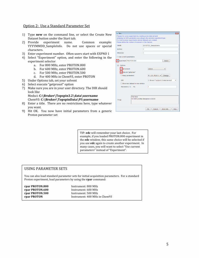
Option 2: Use a Standard Parameter Set

1) Type new on the command line, or select the Create New Dataset button under the Start tab.

2) Provide experiment name. Common example: YYYYMMDD_SampleInfo. Do not use spaces or special characters.

3) Enter experiment number. Often users start with EXPNO 1 4) Select “Experiment” option, and enter the following in the

experiment selector a. For 800 MHz, enter PROTON.800 b. For 600 MHz, enter PROTON.600 c. For 500 MHz, enter PROTON.500 d. For 400 MHz in Chem93, enter PROTON

5) Under Options tab, set your solvent 6) Select execute “getprosol” option 7) Make sure you are in your user directory. The DIR should

look like Medsci: C:\Bruker\Topspin3.2\data\username Chem93: C:\Bruker\TopspinData\PI\username

8) Enter a title. There are no restrictions here, type whatever you want.

9) Hit OK. You now have initial parameters from a generic Proton parameter set

TIP: edc will remember your last choice. For example, if you loaded PROTON.800 experiment in the edc window, this same choice will be selected if you use edc again to create another experiment. In many cases, you will want to select “Use current parameters” instead of “Experiment”.

USING PARAMETER SETS You can also load standard parameter sets for initial acquisition parameters. For a standard Proton experiment, load parameters by using the rpar command: rpar PROTON.800 Instrument: 800 MHz rpar PROTON.600 Instrument: 600 MHz rpar PROTON.500 Instrument: 500 MHz rpar PROTON Instrument: 400 MHz in Chem93

6

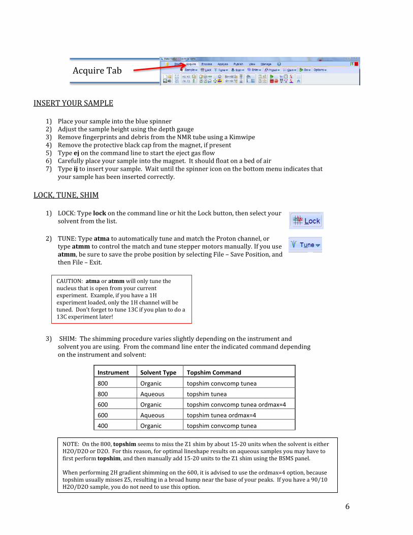
INSERT YOUR SAMPLE 1) Place your sample into the blue spinner 2) Adjust the sample height using the depth gauge 3) Remove fingerprints and debris from the NMR tube using a Kimwipe 4) Remove the protective black cap from the magnet, if present 5) Type ej on the command line to start the eject gas flow 6) Carefully place your sample into the magnet. It should float on a bed of air 7) Type ij to insert your sample. Wait until the spinner icon on the bottom menu indicates that

your sample has been inserted correctly.

LOCK, TUNE, SHIM

1) LOCK: Type lock on the command line or hit the Lock button, then select your solvent from the list.

2) TUNE: Type atma to automatically tune and match the Proton channel, or type atmm to control the match and tune stepper motors manually. If you use atmm, be sure to save the probe position by selecting File – Save Position, and then File – Exit.

3) SHIM: The shimming procedure varies slightly depending on the instrument and

solvent you are using. From the command line enter the indicated command depending on the instrument and solvent:

Instrument Solvent Type Topshim Command

800 Organic topshim convcomp tunea

800 Aqueous topshim tunea

600 Organic topshim convcomp tunea ordmax=4

600 Aqueous topshim tunea ordmax=4

400 Organic topshim convcomp tunea

CAUTION: atma or atmm will only tune the nucleus that is open from your current experiment. Example, if you have a 1H experiment loaded, only the 1H channel will be tuned. Don’t forget to tune 13C if you plan to do a 13C experiment later!

Acquire Tab

NOTE: On the 800, topshim seems to miss the Z1 shim by about 15-20 units when the solvent is either H2O/D2O or D2O. For this reason, for optimal lineshape results on aqueous samples you may have to first perform topshim, and then manually add 15-20 units to the Z1 shim using the BSMS panel. When performing 2H gradient shimming on the 600, it is advised to use the ordmax=4 option, because topshim usually misses Z5, resulting in a broad hump near the base of your peaks. If you have a 90/10 H2O/D2O sample, you do not need to use this option.

7

CHECK ACQUISITION PARAMETERS

1) Type ased on the command line. This will display the important acquisition parameters

in a condensed table. To access all of the acquisition parameters, type eda on the command line.

2) Modify acquisition parameters if desired.

CHECK RECEIVER GAIN

1) Type rga on the command line to automatically set the receiver gain, or hit the Gain button

ACQUIRE YOUR DATA

1) Type zg on the command line, or select the Go button.

Sweep Width, in Hz and in ppm

Carrier Frequency in ppm. Center of your spectrum

Number of scans

Number of points collected. Usually 32k or 64k

Relaxation Delay, usually 2 seconds for zg30

Pulse Program. zg30 means 30° hard pulse, and acquire

90° pulse length and power. The getprosol command will populate these values for you. You can also use the command pulsecal, which will find the accurate 90° pulse length for your specific sample.

8

INITIAL DATA PROCESSING

1) Navigate to the Process tab 2) Perform a weighted Fourier transform by typing efp on the command line. Check the

exponential weighting factor by typing lb. Typical weighting factors for 1H NMR are 0 to 0.3 Hz.

3) Perform automatic phasing of your data by typing apk on the command line 4) View your full spectral window by typing .all on the

command line, or by using the navigation buttons.

MANUAL PHASE ADJUSTMENT

1) Often times, automatic phasing will not do an adequate job. To perform manual phasing,

select the Adjust Phase button, or type .ph on the command line 2) Set the pivot point to either the most upfield or the most downfield resonance: right-

click on the peak, and select Set Pivot Point 3) Use the 0 order to phase the peaks near the Pivot Point, and the 1 order to phase the

other peaks.

Process Tab

NOTE: You can also select the Proc Spectrum button, which will perform efp, then apk, and finally an automatic baseline correction abs. You can change the exponential weighting factor by typing lb into the command line. Typically, one uses 0.1 to 0.3 Hz exponential weighting.

Right click on the most upfield or most downfield peak, and select Set Pivot Point.

To phase, click and hold the 0 or the 1 order phase, and move up or down. Use the 0 order for the peaks near the pivot point, and use the 1 order for the remainder of the peaks.

When you are done, hit the save and close button.

9

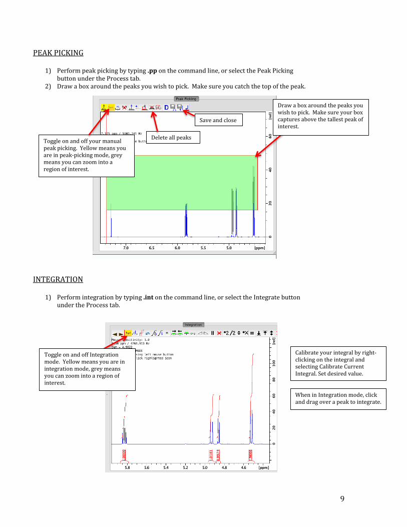
PEAK PICKING

1) Perform peak picking by typing .pp on the command line, or select the Peak Picking button under the Process tab.

2) Draw a box around the peaks you wish to pick. Make sure you catch the top of the peak.

INTEGRATION

1) Perform integration by typing .int on the command line, or select the Integrate button

under the Process tab.

Draw a box around the peaks you wish to pick. Make sure your box captures above the tallest peak of interest.

Toggle on and off your manual peak picking. Yellow means you are in peak-picking mode, grey means you can zoom into a region of interest.

Save and close

Delete all peaks

Toggle on and off Integration mode. Yellow means you are in integration mode, grey means you can zoom into a region of interest.

When in Integration mode, click and drag over a peak to integrate.

Calibrate your integral by right-clicking on the integral and selecting Calibrate Current Integral. Set desired value.

10

REMOVE YOUR SAMPLE

1) Type ej on the command line 2) Remove your sample, and place the black cap onto the bore of the magnet 3) Type ij to stop the air flow. Do not insert any blank sample 4) Place the empty spinner in the sample holder for the next user

UPLOAD YOUR DATA TO GOOGLE DRIVE

To manually copy your data to Google Drive:

1) Open up a Windows Explorer and navigate to the google drive folder for your PI: 800 MHz: C:\\Bruker\NMR-DRIVE\MSD-Bru800\Principleinvestigator600

2) Open up a second Windows Explorer, and navigate to your Bruker data directory: C:\\Bruker\Topspin3.2\data\username

3) Find the experiment names in your user directory that you wish to copy to google drive 4) Copy, or drag and drop to your data to your google drive folder

COPY YOUR DATA TO KONA (OPTION 2)

5) Open up a Windows Explorer and navigate to the Shared drive, S:\\Share$ 6) Open up a second Windows Explorer, and navigate to your Bruker data directory:

C:\\Bruker\Topspin3.2\data\username 7) Find the experiment names in your user directory that you wish to copy to KONA 8) Copy, or drag and drop to your data to your KONA folder

LOGOUT AND SIGN LOGBOOK

1) Close Topspin 3.2 and any other applications 2) Log out of your account using the Start Menu 3) Sign the logbook 4) Report your time using the online billing form.

a) Instructions for online time reporting found here

Exit Procedure

Before uploading your data to KONA, please first delete your processed data. Your raw data will be untouched, and you can re-process your data at any time.

Note, if you are using the 600 or 800 MHz systems at MSD1, you can configure your topspin account to auto-archive your data to google drive. Follow these instructions to set up this feature

http://www.nmr.ucdavis.edu/forms/index.html

11

Experiment: Routine Carbon NMR

Instrument: 800 Medsci, 600 Medsci, 400 Chem

Before collecting 13C NMR, it is suggested you first collect a routine 1H experiment. Follow the procedures starting on page 2. After you have collected your Proton NMR experiment, and saved your data, you can proceed with 13C NMR setup and acquisition.

Note, for 13C NMR you will need at least 10 mg to obtain decent signal to noise in a reasonable timeframe. Dissolve your sample in an appropriate deuterated NMR solvent. Make sure there is no un-dissolved material. If there is, you will need to either centrifuge or filter your sample to remove crystals/debris.

SAMPLE PREPARATION

LOGIN AND STARTUP

INSERT YOUR SAMPLE

LOCK, SHIM

CREATE DATASET / SET INITIAL PARAMETERS

1) From your Proton experiment, create a new identical experiment in EXPNO 2 by typing edc

or new on the command line, or by hitting the Create Dataset button. Make sure the Options tab is opened to display all setup options. Just keep the settings the same as from when you created your Proton experiment -- your goal here is simply to create a place for your data, not to load any parameters.

2) Load standard CARBON acquisition and processing parameters by loading the relevant parameter set and executing getprosol:

If you have not already collected a Proton NMR experiment, follow procedures in the Routine Proton guide. Make sure you have tuned 13C in addition to 1H.

CARBON-13 PARAMETER SETS rpar CARBON.800 all; getprosol Instrument: 800 MHz rpar CARBON.600 all; getprosol Instrument: 600 MHz rpar CARBON.500 all; getprosol Instrument: 500 MHz rpar C13CPD all; getprosol Instrument: 400 MHz

Start Tab

12

TUNE

1) You previously tuned the 1H coil, but not the 13C coil. Type atma or atmm on the command line. Note, when you use atma or atmm, Topspin knows which nuclei you are using based on your acquisition parameters. For example, when the CARBON experiment is loaded, atma will tune both 1H and 13C coils.

CHECK ACQUISITION PARAMETERS

2) Type ased on the command line to check the condensed version of your acquisition parameters. Pay attention to the following parameters:

3) Check your experiment time by typing expt on the command line, or by hitting the Time button. Adjust your acquisition parameters if necessary

ACQUIRE YOUR DATA

1) To start data acquisition, type zg on the command line, or hit Go.

Note, you can perform a Fourier transform during acquisition so that you don’t have to wait until the experiment has completed to observe your data. To perform a Fourier transform while your data is acquiring, you must first transfer the FID so that it can be processed. Type tr on the command line. After a couple additional scans your data will be transferred and ready for processing. Type efp to view your transferred data.

2) If you are satisfied with your signal to noise before your experiment has completed, you can

stop data acquisition by typing stop (more harsh) or halt (less harsh) on the command line, or by hitting the Stop or Halt buttons. If you use halt, you can continue acquisition later.

Acquire Tab

Parameter Description Suggested Value ns Number of scans 512 is default. Depends on your sample concentration ds Dummy scans 4 sw Spectral Width 240 ppm td Number of acquired points 32k d1 relaxation delay 1 second for most cases o1p 13C Offset Frequency 110 ppm, or center of your spectrum o2p 1H Decoupler Offset Freq 5 ppm, or center of your Proton spectrum

13

INITIAL DATA PROCESSING

1) Check your SI (number of points used during Fourier transform) by typing si on the command line. Make sure that si is at least the number of td points, in this case 32k.

2) Check your line broadening function for the Fourier transform by typing lb on the command line. Set lb to 0.5 or 1 Hz.

3) Perform Weighted Fourier transform by typing efp on the command line 4) Perform automatic phasing of your data by typing apk on the command line 5) View your full spectral window by typing .all on the command line, or by using the navigation

buttons.

MANUAL PHASE ADJUSTMENT Often, apk does not do an adequate job with phasing your data, especially if there is probe ring-down or background signal (evident as a broad hump in your 13C spectrum). You can manually adjust the phasing of your C13 spectrum in the same manor as for H1 phase adjustment. See Manual Phase Adjustment section in the Proton guide for details. Briefly, first phase the upfield peaks using ph 0, then phase the downfield peaks using ph 1. You may need to iterate back and fourth between 0 and 1 for best results.

PEAK PICKING Perform 13C Peak Picking in the same manor as for your 1H experiment. See Peak Picking in the Proton guide for details.

PLOTTING To create a hard plot, navigate to the Publish tab. Here you can print a paper copy by hitting the Plot button, or electronic PDF copy with the PDF button.

SAVE YOUR DATA TRANSFER YOUR DATA TO KONA or GOOGLE DRIVE REMOVE YOUR SAMPLE LOGOUT AND SIGN LOGBOOK

Process Tab

Follow instructions in the Routine Proton user guide for how to save and archive your data, and for proper exit procedures.

14

Experiment: Routine 2D NMR Experiments: COSY, HSQC, HMBC, H2BC

Instrument: Bruker 800 and 600 (MedSci), Bruker 400 (Chem)

Before you start: Tuning: It is extremely important that you tune and match the probe for all nuclei used in your experiments before acquiring any 2D NMR experiment. These 2D pulse programs rely on accurate 90 and 180 pulses, and if the probehead is not tuned for your specific sample, these pulses will not be correct. One of the most common mistakes is for users to first load a Proton experiment, correctly lock, tune, shim, acquire, and then load a Carbon or 2D experiment and forget to tune the 13C channel. Be sure to execute atmm or atma after you have loaded any experiment using the X-channel, 90 Pulses: In most cases, assuming you have tuned the probe, the default pulselengths will work for your sample. You can make sure you have loaded the default pulselengths and powers by executing the command getprosol. However, sometimes even if the probe is tuned properly, the default pulse lengths will not be accurate. Thus, you may benefit from identifying accurate 90 and 180 pulselengths before data acquisition. The most efficient way to calibrate pulselengths specifically for your sample is to execute the command pulsecal. The pulsecal command will automatically determine your 90 and 180 pulselengths, and then input them as acquisition parameters in your NMR experiment. This procedure typically only takes about 30 seconds, so it is highly recommended!

COSY HSQC

15

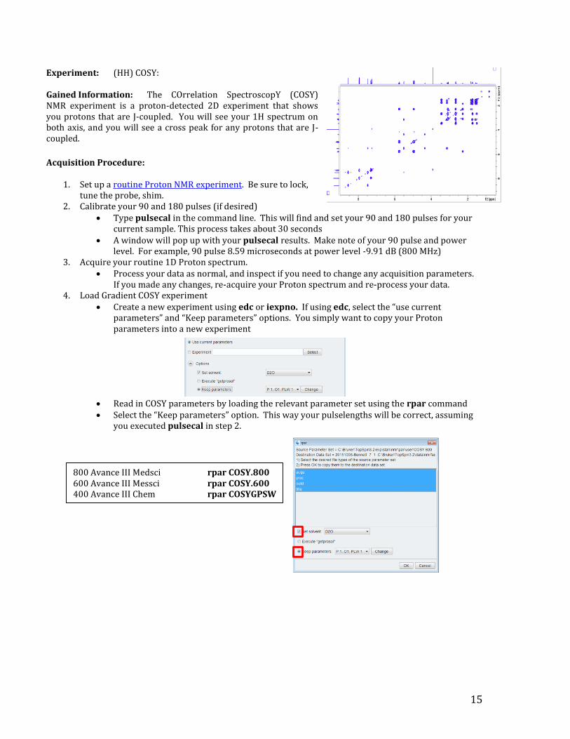
Experiment: (HH) COSY: Gained Information: The COrrelation SpectroscopY (COSY) NMR experiment is a proton-detected 2D experiment that shows you protons that are J-coupled. You will see your 1H spectrum on both axis, and you will see a cross peak for any protons that are J-coupled.

Acquisition Procedure:

1. Set up a routine Proton NMR experiment. Be sure to lock, tune the probe, shim.

2. Calibrate your 90 and 180 pulses (if desired) Type pulsecal in the command line. This will find and set your 90 and 180 pulses for your

current sample. This process takes about 30 seconds A window will pop up with your pulsecal results. Make note of your 90 pulse and power

level. For example, 90 pulse 8.59 microseconds at power level -9.91 dB (800 MHz) 3. Acquire your routine 1D Proton spectrum.

Process your data as normal, and inspect if you need to change any acquisition parameters. If you made any changes, re-acquire your Proton spectrum and re-process your data.

4. Load Gradient COSY experiment Create a new experiment using edc or iexpno. If using edc, select the “use current

parameters” and “Keep parameters” options. You simply want to copy your Proton parameters into a new experiment

Read in COSY parameters by loading the relevant parameter set using the rpar command Select the “Keep parameters” option. This way your pulselengths will be correct, assuming

you executed pulsecal in step 2.

800 Avance III Medsci rpar COSY.800 600 Avance III Messci rpar COSY.600 400 Avance III Chem rpar COSYGPSW

16

5. Set your spectral width using Set Limits (Acquire tab)

6. Check the following acquisition parameters. You can see these parameters under AcqPars. Use the

command eda to see all acquisition parameters, or ased to see condensed acquisition parameters. You can also edit each parameter manually by typing the parameter into the command line.

Check your acquisition time by typing expt on the command line, and edit your acquisition parameters if needed.

7. Acquire your data

Type rga on the command line or hit the Gain button to automatically set your receiver gain Type zg on the command line, or hit the Go button to begin data acquisition

Processing Procedure:

1. Check your processing parameters under ProcPar: type edp to edit processing parameters

2. Under the Process tab hit the Proc Spectrum button, or type xfb on the command line

Name Parameter Suggested Value Spectral Width sw 14 ppm, or set with Set Limits Offset Frequency o1p Center of spectrum (use Set Limits) Number of Points td 2048 in F2, 256 points in F1. Check your acquisition time aq, shoot for about 0.2-0.4 sec Acquisition time aq Change number of points in F2 so that aq in F2 is about 0.2 seconds. Relaxation Delay d1 1.5 or 2 seconds Number of Scans ns minimum 1 scan. Depends on your sample concentration Dummy Scans ds For best results use 16 dummy scans

Using SetLimits: Step 1: Hit the SetLimits button under the Acquire tab Step 2: Load your 1D Proton spectrum. Leave the dialog box open for now Step 3: Click and drag to zoom into region of interest Step 4: Hit OK. Your spectral width and carrier frequency in both your F2 and F1 Proton dimensions should now be set based on your selection

Processing Parameters Set number of points si based on your number of points used in acquisition td. For example, if you acquired 2048 in F2 and 256 points in F1, then set SI to 2048 and 2048. You should always process using binary numbers (ie, 512, 1024, 2048, 4096, etc) Set SPECTYP to COSY

17

Experiment: (HC) HSQC: Gained Information: The Heteronuclear Single Quantum Correlation (HSQC) NMR experiment is a proton-detected 2D experiment that shows you 1H / 13C connectivity. You will see your 1H spectrum as your F2 axis and your 13C spectrum as your F1 axis, and you will see a cross peak for any 1H connected to a 13C that is one bond away. The HSQC is often faster to acquire and more informative than the 1D 13C DEPT experiment, and the same information is obtained.


1. Set up a routine Proton NMR experiment. Be sure to lock, tune the probe, shim. 2. Calibrate your 90 and 180 pulses

Type pulsecal in the command line. This will find and set your 90 and 180 pulses for your current sample. This process takes about 30 seconds

A window will pop up with your pulsecal results. Make note of your 90 pulse and power level.

3. Acquire your routine 1D Proton spectrum. Process your data as normal, and inspect if you need to change any acquisition parameters.

If you made any changes, re-acquire your Proton spectrum and re-process your data. 4. Setup and Acquire a Routine Carbon experiment. Be sure to tune the 13C coil

Create a new experiment using edc or iexpno, and acquire 13C data as normal. 5. Load the HSQC experiment parameters

Load your 1D Proton experiment into the workspace (type re 1 if your 1H spectrum is in expno 1)

Create a new experiment using edc. Select the “use current parameters” and “Keep

parameters” options. You simply want to copy your Proton parameters into a new experiment

Read in HSQC parameters by loading the relevant parameter set using the rpar command Select the “Keep parameters” option. This way your pulselengths will be correct, assuming


800 Avance III Medsci rpar HSQC.800 600 Avance III Messci rpar HSQC.600 400 Avance III Chem rpar HSQCEDETGP

18

6. Set your 1H and 13C spectral widths using Set Limits (Acquire tab)








2. Under the Process tab hit the Proc Spectrum button, or type xfb on the command line 3. For advanced 2D Data processing, including phasing and referencing 2D data, see the Advanced

Processing guide.

Name Parameter Suggested Value Spectral Width sw 14 ppm in F2 and 200 ppm in F1, or set with Set Limits Offset Frequency o1p, o2p Center of spectrum (use Set Limits) Number of Points td 2048 in F2, 400 points in F1. Check your acquisition time aq, shoot for about 0.2 sec Acquisition time aq Change number of points in F2 so that aq in F2 is about 0.2 seconds. Relaxation Delay d1 1.5 seconds Number of Scans ns minimum 1 scan. Depends on your sample concentration Dummy Scans ds For best results use 16 or 32 dummy scans

Using SetLimits: Step 1: Hit the SetLimits button under the Acquire tab Step 2: Load your 1D Proton spectrum. Leave the dialog box open for now Step 3: Click and drag to zoom into region of interest Step 4: Hit OK. Your spectral width and carrier frequency in both your direct dimension (F2) is now set based on your selection Step 5: Repeat steps 1 – 4 but this time load your 1D Carbon spectrum. This will set your F1 dimension based on your selection.

Processing Parameters Set number of points si based on your number of points used in acquisition td. For example, if you acquired 2048 in F2 and 400 points in F1, then set SI to 2048 and 2048. You should use the next highest binary numbers (ie, 512, 1024, 2048, 4096, etc) Set SPECTYP to HSQC

19

Experiment: (HC) HMBC: Gained Information: The Heteronuclear Multiple Bond Correlation (HMBC) NMR experiment is a proton-detected 2D experiment that shows you 1H / 13C multiple-bond connectivity. You will see your 1H spectrum as your F2 axis and your 13C spectrum as your F1 axis, and you will see a cross peak for any 1H / 13C pair that are multiple bonds away, typically 3 to 5 bonds.



3. Calibrate your 90 and 180 pulses Type pulsecal in the command line. This will find and set your 90 and 180 pulses for your


level. 4. Acquire your routine 1D Proton spectrum.


5. Setup and Acquire a Routine Carbon experiment. Be sure to tune the 13C coil Create a new experiment using edc or iexpno, and acquire 13C data as normal.

6. Load the HMBC experiment parameters Load your 1D Proton experiment into the workspace (type re 1 if your 1H spectrum is in

expno 1) Create a new experiment using edc. Select the “use current parameters” and “Keep


Read in HMBC parameters by loading the relevant parameter set using the rpar command Select the “Keep parameters” option. This way your pulselengths will be correct, assuming


800 Avance III Medsci rpar HMBC.800 600 Avance III Messci rpar HMBC.600 400 Avance III Chem rpar HMBCETGPL3ND

20




Check your acquisition time by typing expt on the command line, and edit your acquisition parameters if needed. This is an insensitive experiment, plan accordingly!






Processing guide.

Name Parameter Suggested Value Spectral Width sw 10 ppm in F2 and 200 ppm in F1, or set with Set Limits Offset Frequency o1p, o2p Center of spectrum (use Set Limits) Number of Points td 2048 in F2, 400 points in F1. Check your acq time aq, shoot for about 0.3 - 0.4 seconds Acquisition time aq Change number of points in F2 so that aq in F2 is about 0.3 – 0.4 seconds. Relaxation Delay d1 Ideally set to 1.5 times your non-methyl T1 relaxation time. Good guess is 1.3 seconds Number of Scans ns 4 scans if at high sample concentration (> 25 mg/mL). Dummy Scans ds For best results use 16 or 32 dummy scans


Processing Parameters Set number of points si based on your number of points used in acquisition td. For example, if you acquired 2048 in F2 and 400 points in F1, then set SI to 2048 and 2048. You should use the next highest binary numbers (ie, 512, 1024, 2048, 4096, etc) Set SPECTYP to HMBC

21

Experiment: (HC) H2BC: Gained Information: The Heteronuclear 2-Bond Correlation (H2BC) NMR experiment is a proton-detected 2D experiment that shows you 1H / 13C two-bond connectivity, but only for carbons with attached protons. You will see your 1H spectrum as your F2 axis and your 13C spectrum as your F1 axis, and you will see a cross peak for any 1H / 13C pair that are separated by two bonds if the carbon also has attached protons. This experiment often clears up ambiguity in the HMBC data



2. Calibrate your 90 and 180 pulses Type pulsecal in the command line. This will find and set your 90 and 180 pulses for your


level. 3. Acquire your routine 1D Proton spectrum.


4. Setup and Acquire a Routine Carbon experiment. Be sure to tune the 13C coil Create a new experiment using edc or iexpno, and acquire 13C data as normal.

5. Load the H2BC experiment parameters Load your 1D Proton experiment into the workspace (double click in the file browser, or

type re 1 on the command line if your 1H spectrum is in expno 1) Create a new experiment using edc. Select the “use current parameters” and “Keep


Read in H2BC parameters by loading the relevant parameter set using the rpar command Select the “Keep parameters” option. This way your pulselengths will be correct, assuming


800 Avance III Medsci rpar H2BC.800 600 Avance III Messci rpar H2BC.600 400 Avance III Chem rpar H2BC.400

22










Processing guide.

Name Parameter Suggested Value Spectral Width sw 14 ppm in F2 and 200 ppm in F1, or set with Set Limits Offset Frequency o1p, o2p Center of spectrum (use Set Limits) Number of Points td 4096 in F2, 256 points in F1. Check your acq time aq, shoot for about 0.3 – 0.4 sec Acquisition time aq Change number of points in F2 so that aq in F2 is about 0.3 – 0.4 seconds. Relaxation Delay d1 1.5 seconds Number of Scans ns Minimum 2 scans, but use as many as possible in allowed time. Dummy Scans ds For best results use 16 or 32 dummy scans


Processing Parameters Set number of points si based on your number of points used in acquisition td. For example, if you acquired 2048 in F2 and 400 points in F1, then set SI to 2048 and 2048. You should use the next highest binary numbers (ie, 512, 1024, 2048, 4096, etc) Set SPECTYP to H2BC

23

Experiment: Advanced 1D Experiments: T1, T2, Homonuclear Decoupling, 1D NOE

Instrument: Bruker 800 and 600 (MedSci), Bruker 400 (Chem)

Experiment: Measuring 1H T1 relaxation times: T1 Inversion Recovery experiment Gained Information: This experiment will give you T1 relaxation times for all resonances in your Proton spectrum. This information is especially important if you wish to collect quantitative NMR spectra, where you will need to wait at least 5x T1 of your slowest relaxing peak. Acquisition Procedure:

1. Collect a routine 1H NMR spectrum. Be sure to lock, tune the probe, shim. Process your 1H NMR spectrum, and make sure you can view all of your peaks. Optimize

proton acquisition parameters if necessary including spectral width, number of scans, carrier frequency, and acquisition time.

2. Create a new experiment with optimized parameters from Experiment 1 Say you collected 1H in experiment 1. Copy these experimental parameters over to the next

available experiment (experiment 2) by typing iexpno on the command line. Alternatively, type edc, enter an experiment number of choice, select use current parameters, hit OK. Experiment 2 should be identical to Experiment 1.

3. Load the T1 Inversion Recovery parameters using an rpar (Read Parameters) Type the following into the Topspin command line, depending on which instrument you are

using:

Select Set Solvent and Execute getprosol 4. Calibrate your 90 and 180 pulses

Type pulsecal in the command line. This will find and set your 90 and 180 pulses for your current sample. This process takes about 30 seconds, and you will see a window when it is done listing your calibrated 90 degree pulses at relevant powers.

5. Set your spectral width using the SetLimits option (See Using SetLimits in the 2D guide for help) Under the Acquire tab, hit the SetLimits button With the dialog box still open, navigate to and open your Proton spectrum from Step 1. Click and drag to set your spectral width approximately 1 ppm on either side of your most

upfield and most downfield peaks. Hit OK, and you will see a message stating that your spectral width SW and your offset

frequency O1P has been changed. 6. Check your acquisition paramters:

Type ased or eda on the command line, and check the following acquisition parameters:

7. Set Receiver Gain using rga or with the Gain button 8. Acquire your data by typing zg or by selecting the Go button.

800 Avance III Medsci rpar T1.800 600 Avance III Messci rpar T1.600 400 Avance III Chem rpar T1.400

Name Parameter Suggested Value Spectral Width sw 14 ppm, or set with Set Limits Offset Frequency o1p Center of spectrum (use Set Limits) Number of Points td 32k in F2, 8 points in F1. Must match number of points in vdlist Relaxation Delay d1 use 5 times T1. Default is 20 seconds Number of Scans ns Use at least 2 scans Dummy Scans ds For best results use 4, but you can set this to 2 or 0 if you just want a crude estimate Variable Delay List vdlist T1_8 Edit or load the delay list. Must match TD in F1.

24

Data Processing Procedure for T1 Experiments:

1. Navigate to the Process tab 2. Check your processing parameters (type edp, or select ProcPars).

You should set si equal to td in both F1 and F2. For example, si should be set to 32k in F2 and 8 in F1, matching the number of acquired points (td) in both dimensions. Note that even if you are not using a power of 2 for td in F1, you must process out to the next highest power of 2 for F1, (si = 8, 16, 32, 64, etc).

Set SPECTYP to PSEUDO2D. 3. Perform 2D Fourier Transform

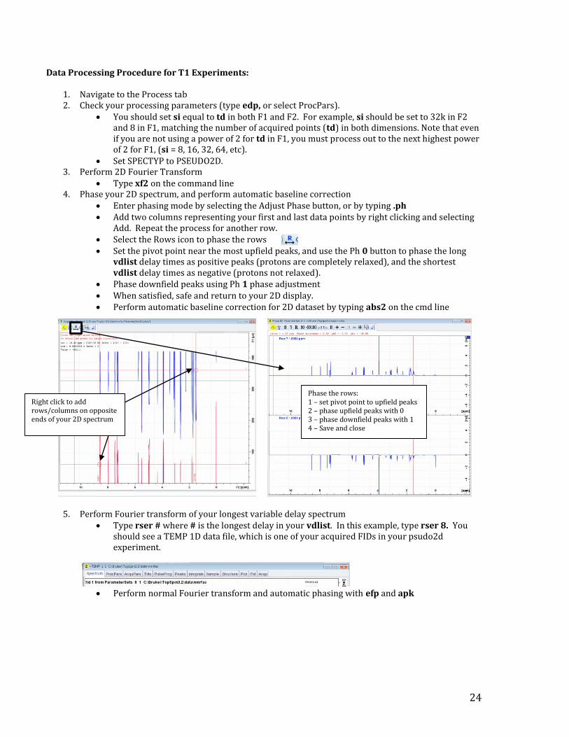
Type xf2 on the command line 4. Phase your 2D spectrum, and perform automatic baseline correction

Enter phasing mode by selecting the Adjust Phase button, or by typing .ph Add two columns representing your first and last data points by right clicking and selecting

Add. Repeat the process for another row. Select the Rows icon to phase the rows Set the pivot point near the most upfield peaks, and use the Ph 0 button to phase the long

vdlist delay times as positive peaks (protons are completely relaxed), and the shortest vdlist delay times as negative (protons not relaxed).

Phase downfield peaks using Ph 1 phase adjustment When satisfied, safe and return to your 2D display. Perform automatic baseline correction for 2D dataset by typing abs2 on the cmd line

5. Perform Fourier transform of your longest variable delay spectrum

Type rser # where # is the longest delay in your vdlist. In this example, type rser 8. You should see a TEMP 1D data file, which is one of your acquired FIDs in your psudo2d experiment.

Perform normal Fourier transform and automatic phasing with efp and apk

Right click to add rows/columns on opposite ends of your 2D spectrum

Phase the rows: 1 – set pivot point to upfield peaks 2 – phase upfield peaks with 0 3 – phase downfield peaks with 1 4 – Save and close

25

6. Set your integration regions (use for peak area determination of T1) Enter integration mode, and integrate all resonances for which you wish to calculate T1 Export your integral regions to the Relaxation module using Save Regions As -> Export

Regions to Relaxation Module and .ret Close out of this Temporary 1D mode and return to your 2D data set.

7. Pick your peaks (use for peak intensity determination of T1)

Repeat step 5, then enter peak picking mode Use manual peak picking to select peaks you wish to analyze for T1 relaxation times. Export your peak list to the Relaxation module using Save Regions As -> Export Regions and

biggest peak within region to Relaxation Module and .ret Close out of this Temporary 1D mode and return to your 2D data set.

8. Enter Relaxation Module for T1 Extraction Navigate to the Analyze tab, select T1/T2 Module, and select T1T2

Select Relaxation button. Note, you have already defined ranges using the integrations or peak picking in Step 6 / Step 7.

Check the Settings, and select uxnmrt1 and vdlist as Function Type and List Name

Select either Area (if you would like to use integrations) or Intensity (if you would like to use your picked peaks)

9. Fit your data and extract T1 for each region

Select that “Calculate Fits for All Peaks” icon.

Observe the results of the fit for each selected peak by cycling through your peaks using the + or – options.

Define integration regions, then export regions to relaxation module. Each defined integration region will be analyzed for T1 relaxation times.

For T1, set Function Type to uxnmrt1, and List File to vdlist

26

Experiment: Measuring 1H T2 relaxation times: CPMG experiment Gained Information: Measure T2 relaxation time for each of your proton resonances in your spectrum. Procedure to Acquire Data:

1. Collect a routine 1H NMR spectrum. Be sure to lock, tune the probe, shim. Process your 1H NMR spectrum, and make sure you can view all of your peaks. Optimize

proton acquisition parameters if necessary including spectral width, number of scans, carrier frequency, and acquisition time.

2. Create a new experiment with optimized parameters from Experiment 1 Say you collected 1H in experiment 1. Copy these experimental parameters over to the next

available experiment (experiment 2) by typing iexpno on the command line. Alternatively, type edc, enter an experiment number of choice, select use current parameters, hit OK.

3. Load the T2 CPMG acquisition and processing parameters using an rpar Type the following into the VnmrJ command line, depending on which instrument you are

using:

Select Set Solvent and Execute getprosol 4. Calibrate your 90 and 180 pulses

Type pulsecal in the command line. This will find your 90 and 180 pulses for your current sample.

5. Set your spectral width using the Set Limits option (See Using SetLimits in the COSY guide for help) Under the Acquire tab, hit the SetLimits button With the dialog box still open, load your Proton spectrum from Step 1 into the workspace. Click and drag to set your spectral width approximately 1 ppm on either side of your most

upfield and most downfield peaks. Hit OK, and you will see a message stating that your spectral width SW and your offset

frequency O1P has been changed. 6. Check your acquisition parameters:

Type ased or eda on the command line, and check the following acquisition parameters:

7. Set Receiver Gain using rga or with the Gain button 8. Acquire your data by typing zg or by selecting the Go button.

800 Avance III Medsci rpar T2.800 600 Avance III Messci rpar T2.600 400 Avance III Chem rpar T2.400

Name Parameter Suggested Value Spectral Width sw 14 ppm, or set with Set Limits Offset Frequency o1p Center of spectrum (use Set Limits) Number of Points td 32k in F2, 8 points in F1. Must match number of points in vdlist Relaxation Delay d1 use 5 times T1. Default is 20 seconds Number of Scans ns Use at least 2 scans Dummy Scans ds For best results use 4, but you can set this to 2 or 0 if you just want a crude estimate Echo time d20 0.5 ms in most cases Variable Delay List vclist T2_8 This list has 8 variable counters, so TD in F1 should be set to 8.

27

Data Processing Procedure for T2 Experiments: Note: this is similar to T1 Processing, with minor variations.

1. Navigate to the Process tab 2. Check your processing parameters (type edp, or select ProcPars).

You should set si equal to td in both F1 and F2. For example, si should be set to 16k in F2 and 8 in F1, matching the number of acquired points (td) in both dimensions. Note that even if you are not using a power of 2 for td in F1, you must process out to the next highest power of 2 for F1, (si = 8, 16, 32, 64, etc).

Check that SPECTYP is set to PSEUDO2D. 3. Perform 2D Fourier Transform

Type xf2 on the command line 4. Phase your 2D spectrum, and perform automatic baseline correction

Enter phasing mode by selecting the Adjust Phase button, or by typing .ph Add two columns representing your first and last data points by right clicking and selecting

Add. Select the Rows icon to phase the rows Set the pivot point near the most upfield peaks, and phase all peaks positive using Ph0 and

Ph1. When satisfied, save and return to your 2D display. Perform automatic baseline correction for 2D dataset by typing abs2 on the cmd line

5. Perform Fourier transform of your shortest echo time experiment in your vclist Type rser # where # is the smallest value in your vclist. In this example, type rser 1. You

should see a TEMP 1D data file, which is one of your acquired FIDs in your psudo2d experiment.

Perform normal Fourier transform and automatic phasing with efp and apk 6. Set your integration regions (use for peak area determination of T2)

Enter integration mode, and integrate all resonances for which you wish to calculate T2 Export your integral regions to the Relaxation module using Save Regions As -> Export

Regions to Relaxation Module and .ret Close out of this Temporary 1D mode and return to your 2D data set.

7. Pick your peaks (use for peak intensity determination of T2)

Repeat step 5, then enter peak picking mode Use manual peak picking to select peaks you wish to analyze for T2 relaxation times. Export your peak list to the Relaxation module using Save Regions As -> Export Regions and

biggest peak within region to Relaxation Module and .ret Close out of this Temporary 1D mode and return to your 2D data set.

8. Convert your T2 couter list vclist into a time list vdlist Type t2convert on the command line, and hit OK through any messages. This macro will

calculate the total echo time for each of your items in the vclist and save as a new vdlist. You later will use this calculated vdlist to fit your T2 decays

Define integration regions, then export regions to relaxation module. Each defined integration region will be analyzed for T1 relaxation times.

28

9. Enter Relaxation Module for T2 Extraction Navigate to the Analyze tab, select T1/T2 Module, and select T1T2

Select Relaxation button. Note, you have already defined ranges using the integrations or peak picking in Step 6 / Step 7.

Check the Settings, and select uxnmrt2 and vdlist as Function Type and List Name. Note, this will only work properly if you have executed the t2convert macro (Step 8)

Select either Area (if you would like to use integrations) or Intensity (if you would like to use your picked peaks)

10. Fit your data and extract T2 for each region Select that “Calculate Fits for All Peaks” icon. Observe the results of the fit for each selected peak by cycling through

your peaks using the + or – options.

For T2, set Function Type to uxnmrt2, and List File to vdlist

29

Experiment: 1D Selective NOE Experiment Gained Information: The selective NOE experiment is commonly used to determine stereochemistry; one selectively excites a proton resonances and observes NOE transfer to nearby protons. Typically, one observes NOE peaks for proton resonances that are in a relatively rigid environment that are within 5 Angstroms of each other. Assuming you are only trying to identify NOEs for a select few resonances, this experiment is often much faster than the 2D NOESY. With any NOE experiment, you need to keep in mind that NOE depends on the molecular tumbling rate, so molecular weight is an important factor in choosing both your experiment and your acquisition parameters. NOE will be positive for small molecules (under 600 Daltons), go through a zero for medium-sized molecules (700 to 1500 Da), and become negative for larger molecules (greater than 1500 Da). For medium-sized molecules, you should try the Selective ROESY experiment, since ROE is always non-zero. You should choose your NOE mixing time based on your molecular weight. As a starting point, for small molecules try a mixing time of 0.5 seconds, medium sized molecules try 0.3 seconds, and large molecules try 0.1 seconds. Acquisition Procedure:

1. Set up routine Proton NMR acquisition. Be sure to lock, tune the probe, shim. Optimize proton acquisition parameters if necessary including spectral width, number of

scans, relaxation delay, carrier frequency, and acquisition time. 2. Calibrate your 90 and 180 pulses



If you made any changes, re-acquire your Proton data and re-process your data. 4. Setup Selective 1D Gradient NOESY experiment: Define Regions

Under the Acquire tab, select Options / Setup Selective 1D Expts.

Then select Define Regions. The Integration window should show up.

Define your regions for selective 1D NOE experiments by setting integrals for each resonance for which you intend to collect 1D NOE data. If you select 5 regions, you will end up collecting 5 1D NOE experiments.

Select Save As -> Save Regions to ‘reg’. Now select Save and Return. Your regions

are now defined. 5. Setup Selective 1D Gradient NOESY experiment:

Create Datasets After you have defined regions, select the Create Datasets button Select the Selective Gradient NOESY experiment Set NOE mixing time. For small molecules (under 600 Da) try 0.5 seconds. For medium-sized

molecules try 0.3 seconds, and for large molecules try 0.1 seconds. Choose desired number of scans. Use at least 32, but the more the better.

30

6. Acquire your data: After you have chosen prompted parameters, select Acquire. This will create a new

experiment and collect 1D NOE for each of your chosen regions. Feel free to adjust any acquisition parameters and re-acquire your data (for example number

of scans, spectral width)


1. Initial Data Processing: perform Fourier transform with efp. 2. Phase your data:

Enter manual phasing mode by selecting the Adjust Phase in the Process tab Move the pivot point to the large peak, and use the 0 order phase correction to phase your

large peak negative. Then use the Ph 1 to phase any NOE peaks positive. 3. Perform baseline correction with abs 4. Compare your 1D NOE spectra with your routine Proton spectrum using Multiple Displays:

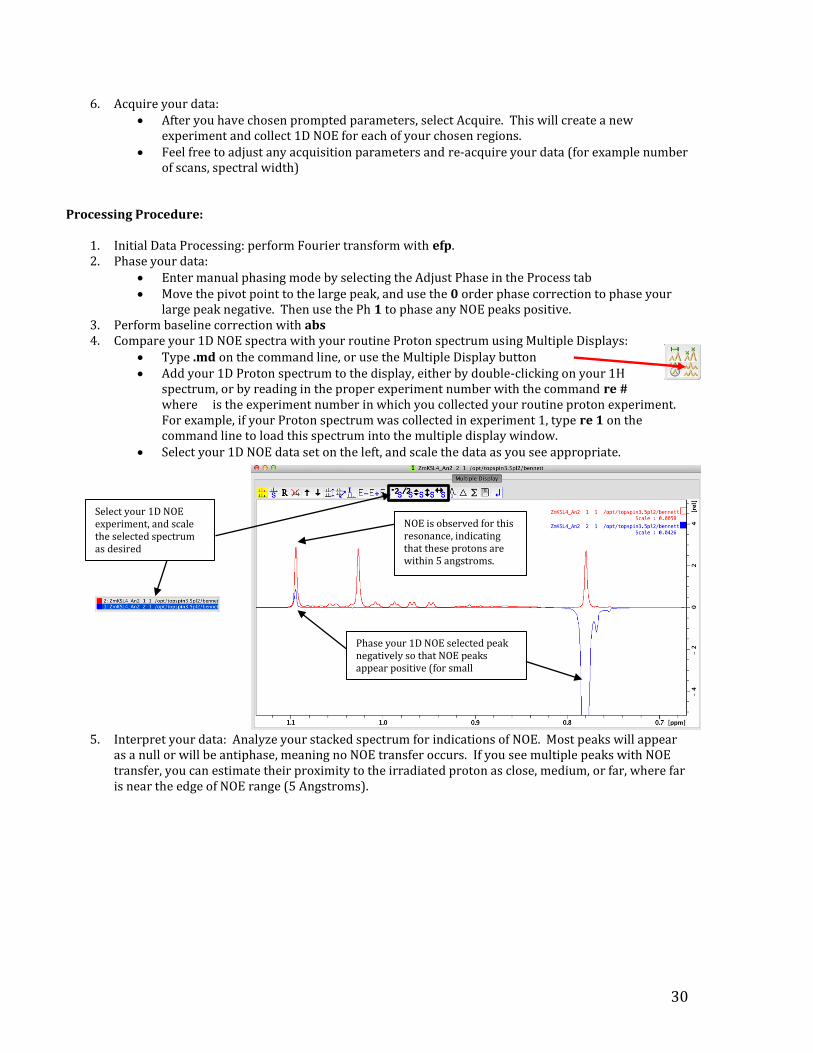
Type .md on the command line, or use the Multiple Display button Add your 1D Proton spectrum to the display, either by double-clicking on your 1H

spectrum, or by reading in the proper experiment number with the command re # where is the experiment number in which you collected your routine proton experiment. For example, if your Proton spectrum was collected in experiment 1, type re 1 on the command line to load this spectrum into the multiple display window.

Select your 1D NOE data set on the left, and scale the data as you see appropriate.

5. Interpret your data: Analyze your stacked spectrum for indications of NOE. Most peaks will appear as a null or will be antiphase, meaning no NOE transfer occurs. If you see multiple peaks with NOE transfer, you can estimate their proximity to the irradiated proton as close, medium, or far, where far is near the edge of NOE range (5 Angstroms).

Select your 1D NOE experiment, and scale the selected spectrum as desired

Phase your 1D NOE selected peak negatively so that NOE peaks appear positive (for small molecules)

NOE is observed for this resonance, indicating that these protons are within 5 angstroms.

31

Experiment: 1D Selective Homonuclear Decoupling Gained Information: The Selective 1D Homonuclear decoupling experiment allows you to acquire a routine Proton spectrum while selectively decoupling a chosen resonance to observe the effect on other resonances. For example, the proton spectrum of Ethanol has a CH3 that appears as a triplet due to the CH2, while the CH2 appears as a quartet due to the CH3. If you selectively decouple the CH3 peak during acquisition, your CH2 peak will collapse into a singlet. Acquisition Procedure:

1. Set up routine Proton NMR acquisition. Be sure to lock, tune the probe, shim. Optimize proton acquisition parameters if necessary including spectral width, number of

scans, relaxation delay, carrier frequency, and acquisition time. 2. Calibrate your 90 and 180 pulses



If you made any changes, re-acquire your Proton data and re-process your data. 4. Setup 1D Homonuclear Decoupling experiment: Define Regions

Under the Acquire tab, select Options / Setup Selective 1D Expts.

Then select Define Regions. The Integration window should show up.

Define your regions for 1D Homonuclear decoupling using the Integration mode: select which resonance or resonances you wish to decouple.

Select Save As -> Save Regions to ‘reg’. Now select Save and Return. Your regions

are now defined. 5. Setup 1D Homonuclear Decoupling experiment:

Create Datasets After you have defined regions, select the

Create Datasets button Select the 1D Homonuclear Decoupling experiment Choose desired number of scans. Use at least 32, but the more the better.

6. Acquire your data: After you have chosen prompted parameters, select Acquire. This will create a new

experiment and collect 1D Homonuclear decoupling spectra for each of your chosen regions.

32


1. Initial Data Processing: perform Fourier transform with efp and phase with apk. 2. Perform baseline correction with abs.

Often the abs command will auto-find integration regions, but will do so not to your liking. In this case, it may be helpful to delete all integrals. To do so, enter integration mode .int and select the Delete All Integrals option, then hit Save and Close

3. Compare your 1D NOE spectra with your routine Proton spectrum using Multiple Displays: Type .md on the command line, or use the Multiple Display button Add your 1D Proton spectrum to the display, either by double-clicking on your 1H

spectrum, or by reading in the proper experiment number with the command re # where is the experiment number in which you collected your routine proton experiment. For example, if your Proton spectrum was collected in experiment 1, type re 1 on the command line to load this spectrum into the multiple display window.

You can choose to either superimpose or stack your spectra with: Select one of your two spectra and scale the data as you see appropriate.

4. Interpret your data: Analyze your stacked spectrum for indications of 1H / 1H decoupling. The resonance that is decoupled will be nulled or severely distorted, while any resonances which are J-coupled to the selected peak will now appear as if no J-coupling is present.

Select one of the two spectra, and scale the selected spectrum as desired

Selectively decoupled resonance

Collapses from a doublet into a singlet: selectively decoupled from resonance at 8.5 ppm

33

Miscellaneous Topics

Disk Utilization: Deleting Processed Data Raw data does not take up much file space, however processed data, especially 2D datasets, can be extremely large files; a couple overnight 2D experiments can easily amount to 300 MB of processed data. Uploading all of this to KONA not only takes a long time, it is also unnecessary. After having a look at your data in Topspin, please consider deleting the processed data from the host computer before uplading to KONA.

Step 1: Type delp from the topspin command line Step 2: Select “Delete the processed data files…” option Step 3: Highlight all processed datasets that you wish to remove. Use Shift or Control to select multiple files Step 4: Hit OK. Your raw data will be untouched, and you can re-process your data at any time.

2D Processed data takes up a lot of space! Each 2ii, 2rr, etc. file is 8 MB.

34

Uploading your data to KONA: You are strongly encouraged to archive all your data using Google Drive or the FTP server (KONA) as soon as each of your NMR runs is completed. Please avoid using USB flash drives because of potential malware/viruses, and please consider the environment when choosing to print. To upload your data to KONA from the Bruker 800 and 600 NMR spectrometers (Windows 7 operating systems), do the following:

1) Open up a Windows Explorer and navigate to the Shared drive, S:\\Share$ 2) Open up a second Windows Explorer, and navigate to your Bruker data directory:

C:\\Bruker\Topspin3.2\data\username 3) Find the experiment names in your user directory that you wish to copy to KONA 4) Copy, or drag and drop to your data to your KONA folder

Retrieving your data from KONA: KONA is an FTP server that can be accessed from any campus IP address. For best results, you should connect via Ethernet using DHCP. You should also be able to connect via mooblenetx and eduroam wifi, however there have been some problems with this method. You should also be able to connect using your lab wifi assuming your wifi router is connected to the campus network via Ethernet.

1) Download and install some FTP client onto your computer, depending on your operating system. Cyberduck and FileZilla are common choices for both windows and mac users.

2) Launch the software, and enter the following information:

Protocol: sftp Server: kona.ucdavis.edu Username: nmrftp Port: 22 Password: Ask for password.

3) Navigate to your directory, and copy your data to your computer.


35

Manually Uploading your data to Google Drive: You are strongly encouraged to archive all your data using Google Drive or the FTP server (KONA) as soon as each of your NMR runs is completed. Please avoid using USB flash drives because of potential malware/viruses, and please consider the environment when choosing to print. To upload your data to Google Drive from the Bruker 800 and 600 NMR spectrometers (Windows 7 operating systems), do the following:

1) Open up a Windows Explorer and navigate to the google drive folder specified for your PI.

800: C:\\Bruker\NMR-DRIVE\MSD-Bru800\PI-800 600: C:\\Bruker\NMR-DRIVE\MSD-Bru600\PI-600

2) Open up a second Windows Explorer, and navigate to your Bruker data directory: C:\\Bruker\Topspin3.2\data\username

3) Find the experiment names in your user directory that you wish to copy to KONA 4) Copy, or drag and drop to your data to your username subfolder within your PIs folder

Retrieving your data from Google Drive: After your PIs folder has been created in the NMR-DRIVE folder, simply ask NMR Facility staff for access to this shared folder. All your data collected on the selected instrument will show up in your UCD google drive account.


If your PIs folder has not been created yet, you may add the directory. As an example, PI John Smith will have a folder on the 800MHz system named Smith800, and each researcher in the Smith lab will have a subdirectory by username.

36

Setting up your Topspin 3.2 Account for the First Time If you are using a spectrometer for the first time, the Topspin interface / layout for your account may not be optimal. To correctly set up your Topspin 3.X interface, take the following steps: Enable Topspin 3 Workflow: When you open up Topspin 3.2 for the first time, your interface/layout will be similar to the old version of topspin: Topspin 1.3. This is the same layout you will see on the 500 and 400 Bruker DRX instruments at Medsci. The newer Topspin 3.2 layout is much better, and it is highly recommended that you enable the new workflow: Step 1: Select Options -> Preferences

Step 2: Enable Topspin 3 Flow and Topspin 3.1 Color/Toolbar Scheme

Step 3: Apply your changes, and close and re-open Topspin 3.2. Your interface should now look like this:

If you would like to revert back to the Topspin 1.3 workflow, go to Manage -> Preferences, and de-select the Topspin 3 options. Apply your changes, close and re-open Topspin.

Check these two options, hit Apply, Close, then close and restart Topspin 3.2

37

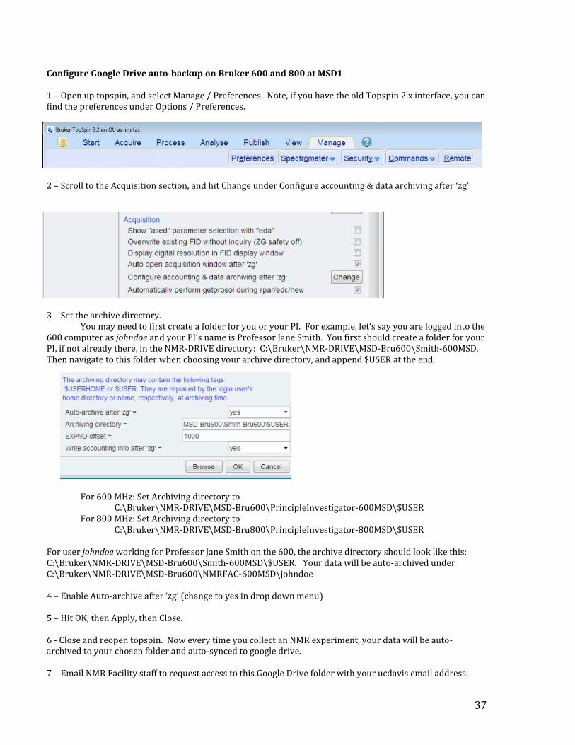
Configure Google Drive auto-backup on Bruker 600 and 800 at MSD1 1 – Open up topspin, and select Manage / Preferences. Note, if you have the old Topspin 2.x interface, you can find the preferences under Options / Preferences.

2 – Scroll to the Acquisition section, and hit Change under Configure accounting & data archiving after ‘zg’

3 – Set the archive directory.

You may need to first create a folder for you or your PI. For example, let’s say you are logged into the 600 computer as johndoe and your PI’s name is Professor Jane Smith. You first should create a folder for your PI, if not already there, in the NMR-DRIVE directory: C:\Bruker\NMR-DRIVE\MSD-Bru600\Smith-600MSD. Then navigate to this folder when choosing your archive directory, and append $USER at the end.

For 600 MHz: Set Archiving directory to

C:\Bruker\NMR-DRIVE\MSD-Bru600\PrincipleInvestigator-600MSD\$USER For 800 MHz: Set Archiving directory to

C:\Bruker\NMR-DRIVE\MSD-Bru800\PrincipleInvestigator-800MSD\$USER For user johndoe working for Professor Jane Smith on the 600, the archive directory should look like this: C:\Bruker\NMR-DRIVE\MSD-Bru600\Smith-600MSD\$USER. Your data will be auto-archived under C:\Bruker\NMR-DRIVE\MSD-Bru600\NMRFAC-600MSD\johndoe 4 – Enable Auto-archive after ‘zg’ (change to yes in drop down menu) 5 – Hit OK, then Apply, then Close. 6 - Close and reopen topspin. Now every time you collect an NMR experiment, your data will be auto-archived to your chosen folder and auto-synced to google drive. 7 – Email NMR Facility staff to request access to this Google Drive folder with your ucdavis email address.

38

Enable Acquisition Status Bar: The Acquisition Status Bar is the region at the bottom of your Topspin software that provides various status information including lock status, temperature, sample status, and generally what the spectrometer is currently doing (ie shimming, acquiring data, etc.) To enable and configure the acquisition status bar, take the following steps: Step 1: Right click on the grey space just below the command line, and select Acquisition Status Bar On/Off

Step 2: When setting Status Bar Preferences, select all options except MAS spinning rate, hit Apply and Close.

Your Acquisition status bar should now be displayed. If it is not displayed after setting your preferences, you may need to right-click again and turn it off, then back on, or you may need to close and re-open topspin.

Sample Status: missing, in magnet, spinning, etc

Lock panel. Double-click to open the large lock display

Read status messages here. For example, “ATMA completed” after tuning, or “topshim completed” after shimming.

Variable Temperature control panel. Type edte or double-click to open the temp control panel.

39

New MedSci 1D Time Reporting Protocol Dear NMR Users, As of February 1st 2016, the paper billing slip has been replaced with an online version. Please follow these instructions to report your NMR usage. Accurate spectrometer usage data is extremely important - this data is pivotal when applying for instrumentation funding, filing for insurance claims in the event of catastrophic hardware failures, and proving our value to the university. Please note, we will compare your self-reported usage to computer logon records and NMR Online Scheduler reservations. Not properly recording your usage will result in suspension of your right to use the equipment. 1: go to the NMR website, nmr.ucdavis.edu 2: select the NMRF Forms tab 3: Under Time Reporting, select the relevant form. If you are a UC Davis user and are self-reporting your usage, use the UC Davis Users – User Run form.

4: If prompted for a Google account, just enter your ucdavis email address. You will then be directed to a Kerberos login screen. Log in with your Kerberos ID and password. Feel free to stay logged in so that you don’t have to log in every time (assuming you logged into the computer using your personal login ID and password, not the nmrfac account) 5: Fill out the appropriate information. If you encountered a problem, report it here. 6: Drag and drop the link onto your desktop so that you can quickly access this form

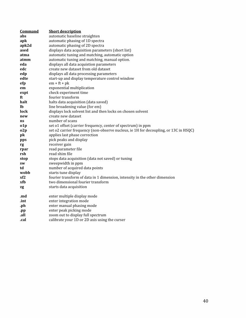
List and Brief Description of Important Commands

40

Command Short description abs automatic baseline straighten apk automatic phasing of 1D spectra apk2d automatic phasing of 2D spectra ased displays data acquisition parameters (short list) atma automatic tuning and matching, automatic option atmm automatic tuning and matching, manual option. eda displays all data acquistion parameters edc create new dataset from old dataset edp displays all data processing parameters edte start-up and display temperature control window efp em + ft + pk em exponential multiplication expt check experiment time ft fourier transform halt halts data acquisition (data saved) lb line broadening value (for em) lock displays lock solvent list and then locks on chosen solvent new create new dataset ns number of scans o1p set o1 offset (carrier frequency, center of spectrum) in ppm o2p set o2 carrier frequency (non-observe nucleus, ie 1H for decoupling, or 13C in HSQC) pk applies last phase correction pps pick peaks and display rg receiver gain rpar read parameter file rsh read shim file stop stops data acquisition (data not saved) or tuning sw sweepwidth in ppm td number of acquired data points wobb starts tune display xf2 fourier transform of data in 1 dimension, intensity in the other dimension xfb two dimensional fourier transform zg starts data acquisition .md enter multiple display mode .int enter integration mode .ph enter manual phasing mode .pp enter peak picking mode .all zoom out to display full spectrum .cal calibrate your 1D or 2D axis using the curser

uc davis nmr facility bruker short manual … uc davis nmr facility bruker short manual for topspin...

Documents