Introduction

Recording all required NMR experiments for a protein structure calculation, dynamic analysis or even backbone assignment can be very time consuming. By using a combination of different techniques for data acquisition and processing, the time required to record almost all experimental data needed to characterize a protein can be shortened significantly.

Looking at a regular NMR experiment, most of the experimental time is spent waiting for the magnetization to recover between scans. This is determined by the spin-lattice relaxation time T1, which is usually of the order of one second for a backbone amide proton in a small- to medium-sized protein. This means that it would take about 5 seconds for 99 % of the magnetization to recover, whereas a usual recovery delay would be in the order of 1.5 seconds (~80 % recovery).

Multidimensional NMR experiments also take significantly longer as, using conventional techniques, introducing an additional dimension usually increases the time necessary to perform an experiment by an order of magnitude. This means that if a two dimensional experiment can be recorded within an hour, a 3D experiment will take a day, 4D a week, 5D a month, and so on. In terms of the signal-to-noise ratio, most of the time – especially when recording high dimensional spectra – a much shorter experiment time is sufficient.

Band-selective excitation and fast repetition

One class of experiments currently used to overcome the problem of long T1 relaxation times is BEST experiments (Band-selective Excitation Short-Transient), developed by Brutscher and co-workers[1,2]. By using band-selective pulses to excite only the backbone amide protons, the majority of proton spins remain untouched and serve as an additional pathway for relaxation. In this case, the selective T1 for the protons of interest is shortened by a factor of three to five. The most simple experiment using this technique is the SOFAST HMQC. Being an HMQC experiment, it is also possible to use Ernst Angle Excitation[3] to further reduce the recovery delay, maximizing the signal-to-noise ratio per time.

It is worth noting that reducing the recovery delay not only shortens the experiment, but at the same time increases the duty cycle; essentially, the same amount of RF power is applied in a much shorter time period. This leads to significant heating of the sample and probe. Although modern CryoProbes™ can handle this increased duty cycle quite well, it is still recommended that short acquisition times and low power nitrogen decoupling are used whenever possible. A typical recommendation is to keep acquisition times below 50 ms and 15N decoupling power at about 750 Hz, which still provides ~40 ppm at 23.3T (950 MHz) using a GARP-4 decoupling sequence[4].

Speeding Up Protein NMR

Daniel MathieuBruker BioSpin GmbH, Rheinstetten, Germany

When going to higher field strengths, it might be worth considering TROSY-based, rather than HSQC-based, experiments[5,6]. The final spectrum will not only show sharper lines, but the experiments also use lower duty cycles, since nitrogen is not decoupled during the acquisition. In addition, more recent work has shown that it is possible to recover steady state 15N magnetization to further increase the sensitivity.

Figure 1

Figure 2

Figure 3

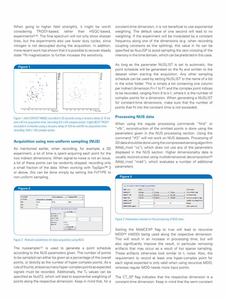
Figure 1: (left) SOFAST HMQC recorded in 20 seconds using a recovery delay of 10 ms and a 40 ms acquisition time, recording 512 x 64 complex points. (right) BEST TROSY recorded in 3 minutes using a recovery delay of 150 ms and 80 ms acquisition time recording 1024 x 128 complex points.

Figure 2: Relevant parameters for data acquisition using NUS.

Figure 3: Parameters relevant to the processing of NUS data.

Acquisition using non-uniform sampling (NUS)

As mentioned earlier, when recording, for example, a 3D experiment, a lot of time is spent acquiring each point for the two indirect dimensions. When signal-to-noise is not an issue, a lot of these points can be randomly skipped, recording only a small fraction of the data. When working with TopSpin™ 3 or above, this can be done simply by setting the FnTYPE to non-uniform sampling.

The nussampler[7] is used to generate a point schedule according to the NUS parameters given. The number of points to be sampled can either be given as a percentage of the overall points, or directly as the number of hyper-complex points. As a rule of thumb, at least as many hyper-complex points as expected signals must be recorded. Additionally, the T2 values can be specified as NusT2, which will lead to exponential weighting of points along the respective dimension. Keep in mind that, for a

constant-time dimension, it is not beneficial to use exponential weighting. The default value of one second will lead to no weighting. If the experiment will be modulated by a constant frequency along one of the dimensions (e.g. when recording coupling constants as line splitting), this value in Hz can be specified as NusJSP to avoid sampling the zero crossing of the intensity in the time domain, which can be predicted in this case.

As long as the parameter NUSLIST is set to automatic, the point schedule will be generated on the fly and written to the dataset when starting the acquisition. Any other sampling schedule can be used by setting NUSLIST to the name of a list in the vclist folder. This is simply a list containing one column per indirect dimension Fn-1 to F1 and the complex point indices to be recorded, ranging from 0 to k-1, where k is the number of complex points for a dimension. When generating a NUSLIST for constant-time dimensions, make sure that the number of points that fit into the constant time is not exceeded.

Processing NUS data

When using the regular processing commands “ftnd” or “xfb”, reconstruction of the omitted points is done using the parameters given in the NUS processing section. Using the command “tf3” will not work on NUS datasets. Processing of 2D data should be done using the compressed sensing algorithm (Mdd_mod “cs”), which does not use any of the parameters displayed in the NUS section. Higher dimensionality data is usually reconstructed using multidimensional decomposition[8] (Mdd_mod “mdd”), which evaluates a number of additional parameters.

Setting the MddCEXP flag to true will lead to recursive MDD[9] (rMDD) being used along the respective dimension. This will result in an increase in processing time, but will also significantly improve the result, in particular removing artifacts that may occur as a result of too sparse sampling. These artifacts otherwise look similar to t1 noise. Also, the requirement to record at least one hyper-complex point for each signal expected is only valid when using recursive MDD, whereas regular MDD needs more input points.

The CT_SP flag indicates that the respective dimension is a constant-time dimension. Keep in mind that the semi-constant

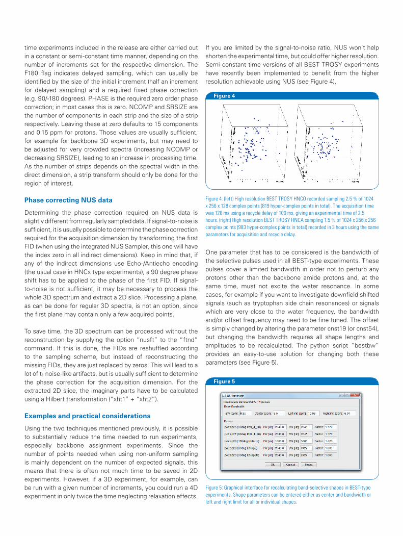
Figure 5

Figure 4: (left) High resolution BEST TROSY HNCO recorded sampling 2.5 % of 1024 x 256 x 128 complex points (819 hyper-complex points in total). The acquisition time was 128 ms using a recycle delay of 100 ms, giving an experimental time of 2.5 hours. (right) High resolution BEST TROSY HNCA sampling 1.5 % of 1024 x 256 x 256 complex points (983 hyper-complex points in total) recorded in 3 hours using the same parameters for acquisition and recycle delay.

Figure 5: Graphical interface for recalculating band-selective shapes in BEST-type experiments. Shape parameters can be entered either as center and bandwidth or left and right limit for all or individual shapes.

Figure 4

time experiments included in the release are either carried out in a constant or semi-constant time manner, depending on the number of increments set for the respective dimension. The F180 flag indicates delayed sampling, which can usually be identified by the size of the initial increment (half an increment for delayed sampling) and a required fixed phase correction (e.g. 90/-180 degrees). PHASE is the required zero order phase correction; in most cases this is zero. NCOMP and SRSIZE are the number of components in each strip and the size of a strip respectively. Leaving these at zero defaults to 15 components and 0.15 ppm for protons. Those values are usually sufficient, for example for backbone 3D experiments, but may need to be adjusted for very crowded spectra (increasing NCOMP or decreasing SRSIZE), leading to an increase in processing time. As the number of strips depends on the spectral width in the direct dimension, a strip transform should only be done for the region of interest.

Phase correcting NUS data

Determining the phase correction required on NUS data is slightly different from regularly sampled data. If signal-to-noise is sufficient, it is usually possible to determine the phase correction required for the acquisition dimension by transforming the first FID (when using the integrated NUS Sampler, this one will have the index zero in all indirect dimensions). Keep in mind that, if any of the indirect dimensions use Echo-/Antiecho encoding (the usual case in HNCx type experiments), a 90 degree phase shift has to be applied to the phase of the first FID. If signal-to-noise is not sufficient, it may be necessary to process the whole 3D spectrum and extract a 2D slice. Processing a plane, as can be done for regular 3D spectra, is not an option, since the first plane may contain only a few acquired points.

To save time, the 3D spectrum can be processed without the reconstruction by supplying the option “nusft” to the “ftnd” command. If this is done, the FIDs are reshuffled according to the sampling scheme, but instead of reconstructing the missing FIDs, they are just replaced by zeros. This will lead to a lot of t1 noise-like artifacts, but is usually sufficient to determine the phase correction for the acquisition dimension. For the extracted 2D slice, the imaginary parts have to be calculated using a Hilbert transformation (“xht1” + “xht2”).

Examples and practical considerations

Using the two techniques mentioned previously, it is possible to substantially reduce the time needed to run experiments, especially backbone assignment experiments. Since the number of points needed when using non-uniform sampling is mainly dependent on the number of expected signals, this means that there is often not much time to be saved in 2D experiments. However, if a 3D experiment, for example, can be run with a given number of increments, you could run a 4D experiment in only twice the time neglecting relaxation effects.

One parameter that has to be considered is the bandwidth of the selective pulses used in all BEST-type experiments. These pulses cover a limited bandwidth in order not to perturb any protons other than the backbone amide protons and, at the same time, must not excite the water resonance. In some cases, for example if you want to investigate downfield shifted signals (such as tryptophan side chain resonances) or signals which are very close to the water frequency, the bandwidth and/or offset frequency may need to be fine tuned. The offset is simply changed by altering the parameter cnst19 (or cnst54), but changing the bandwidth requires all shape lengths and amplitudes to be recalculated. The python script “bestbw” provides an easy-to-use solution for changing both these parameters (see Figure 5).

If you are limited by the signal-to-noise ratio, NUS won’t help shorten the experimental time, but could offer higher resolution. Semi-constant time versions of all BEST TROSY experiments have recently been implemented to benefit from the higher resolution achievable using NUS (see Figure 4).

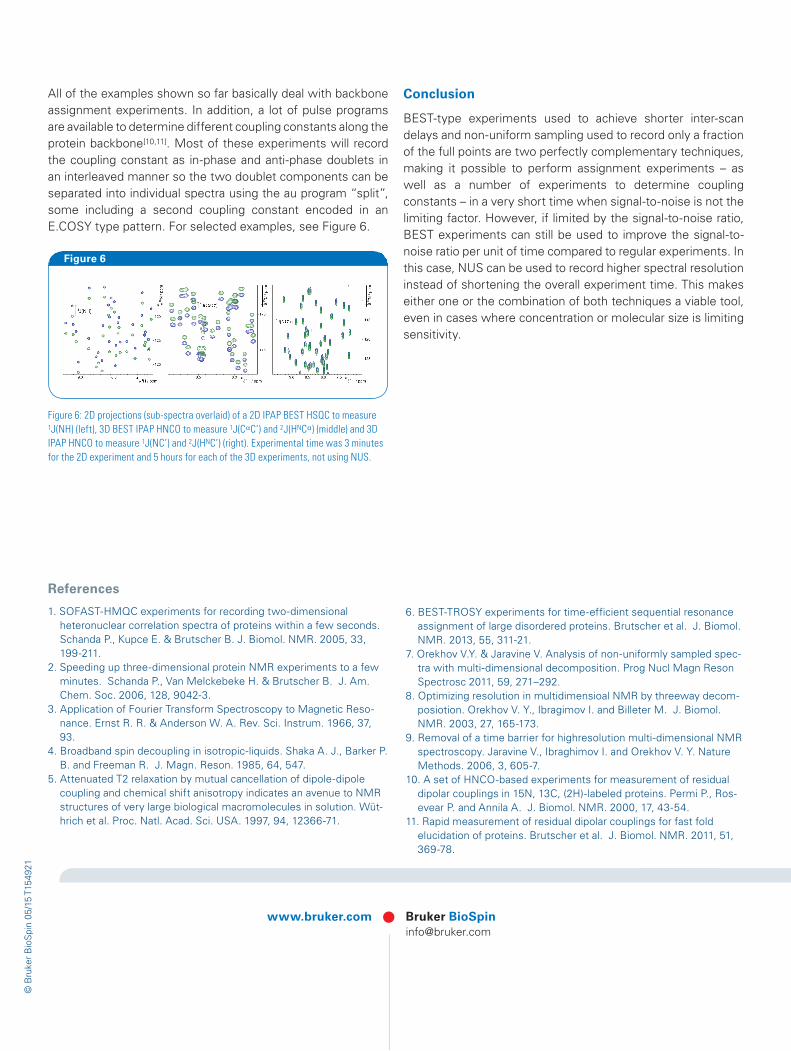
Figure 5

© B

ruke

r B

ioS

pin

05/1

5 T1

5492

1

Bruker BioSpin info@bruker.com

www.bruker.com

References

1. SOFAST-HMQC experiments for recording two-dimensional heteronuclear correlation spectra of proteins within a few seconds. Schanda P., Kupce E. & Brutscher B. J. Biomol. NMR. 2005, 33, 199-211.

2. Speeding up three-dimensional protein NMR experiments to a few minutes. Schanda P., Van Melckebeke H. & Brutscher B. J. Am. Chem. Soc. 2006, 128, 9042-3.

3. Application of Fourier Transform Spectroscopy to Magnetic Reso-nance. Ernst R. R. & Anderson W. A. Rev. Sci. Instrum. 1966, 37, 93.

4. Broadband spin decoupling in isotropic-liquids. Shaka A. J., Barker P. B. and Freeman R. J. Magn. Reson. 1985, 64, 547.

5. Attenuated T2 relaxation by mutual cancellation of dipole-dipole coupling and chemical shift anisotropy indicates an avenue to NMR structures of very large biological macromolecules in solution. Wüt-hrich et al. Proc. Natl. Acad. Sci. USA. 1997, 94, 12366-71.

6. BEST-TROSY experiments for time-efficient sequential resonance assignment of large disordered proteins. Brutscher et al. J. Biomol. NMR. 2013, 55, 311-21.

7. Orekhov V.Y. & Jaravine V. Analysis of non-uniformly sampled spec-tra with multi-dimensional decomposition. Prog Nucl Magn Reson Spectrosc 2011, 59, 271–292.

8. Optimizing resolution in multidimensioal NMR by threeway decom-posiotion. Orekhov V. Y., Ibragimov I. and Billeter M. J. Biomol. NMR. 2003, 27, 165-173.

9. Removal of a time barrier for highresolution multi-dimensional NMR spectroscopy. Jaravine V., Ibraghimov I. and Orekhov V. Y. Nature Methods. 2006, 3, 605-7.

10. A set of HNCO-based experiments for measurement of residual dipolar couplings in 15N, 13C, (2H)-labeled proteins. Permi P., Ros-evear P. and Annila A. J. Biomol. NMR. 2000, 17, 43-54.

11. Rapid measurement of residual dipolar couplings for fast fold elucidation of proteins. Brutscher et al. J. Biomol. NMR. 2011, 51, 369-78.

All of the examples shown so far basically deal with backbone assignment experiments. In addition, a lot of pulse programs are available to determine different coupling constants along the protein backbone[10,11]. Most of these experiments will record the coupling constant as in-phase and anti-phase doublets in an interleaved manner so the two doublet components can be separated into individual spectra using the au program “split”, some including a second coupling constant encoded in an E.COSY type pattern. For selected examples, see Figure 6.

Figure 6

Figure 6: 2D projections (sub-spectra overlaid) of a 2D IPAP BEST HSQC to measure 1J(NH) (left), 3D BEST IPAP HNCO to measure 1J(CαC’) and 2J(HNCα) (middle) and 3D IPAP HNCO to measure 1J(NC’) and 2J(HNC’) (right). Experimental time was 3 minutes for the 2D experiment and 5 hours for each of the 3D experiments, not using NUS.

Conclusion

BEST-type experiments used to achieve shorter inter-scan delays and non-uniform sampling used to record only a fraction of the full points are two perfectly complementary techniques, making it possible to perform assignment experiments – as well as a number of experiments to determine coupling constants – in a very short time when signal-to-noise is not the limiting factor. However, if limited by the signal-to-noise ratio, BEST experiments can still be used to improve the signal-to-noise ratio per unit of time compared to regular experiments. In this case, NUS can be used to record higher spectral resolution instead of shortening the overall experiment time. This makes either one or the combination of both techniques a viable tool, even in cases where concentration or molecular size is limiting sensitivity.