uc davis ec230 1.overview of welfare reform 2.expected effects of

LECTURE: WELFARE REFORM HILARY HOYNES UC DAVIS EC230 OUTLINE OF LECTURE

1.Overview of welfare reform 2.Expected effects of welfare reform 3.Identification of reform effects 4.Impact of Time Limits (Grogger & Michaelopolous) 5.Heterogeneous impacts of reform (Bitler, Gelbach, and Hoynes, Experimental)

WELFARE REFORM IN 1990S Reforms in the 1990s addressed long-standing criticisms that AFDC discourages work and marriage, and causes long term dependence. Two periods of “reform” (1) State waivers – States request HHS to waive specific eligibility and benefit requirements. – Between 1992 and 1996, 28 states were granted major waivers. – Rich variation in timing and nature of waivers (2) FEDERAL REFORM, PRWORA 1996 – Replaces AFDC with TANF (Temporary Assistance for Needy Families) – TANF features: • More state control for program design • Time limit (lifetime limit of 5 years– states can make shorter) • Strengthen work requirements • Financial sanctions • Convert federal funding from matching program to block grant (entitlement

aspect of AFDC gone) – Less variation in TANF implementation dates; still variation in nature of state TANF reforms.

DICHOTOMY OF WELFARE REFORM Welfare

Tightening Welfare Loosening

General Reforms

• Work requirements • Financial sanctions • Time limits

• Liberalize earnings disregards

• Liberalized asset test

Family Structure Specific Reforms

• Family Cap • Residency Requirement

for Unmarried Teens

• Expand eligibility for two-parent families

THEORETICAL PREDICTIONS ABOUT WELFARE REFORM Expected Outcomes: General expected outcomes are: – reduction in welfare caseloads – extensive margin labor supply increase; intensive margin ? – poverty? Could increase or decrease – family structure is unclear

IMPACT OF REFORM ON LABOR SUPPLY Increase in Earnings Disregard (reduction in t)

Hours Worked0

Income

G

1

2

3

Non-working welfare recipients (e.g. 1 above) + employment, hours and earnings – transfer income + income Working welfare recipients

+ (likely) hours, earnings, and transfers + income Newly eligible at prior labor supply (e.g. 2 above)

+ welfare (mechanical response) – hours, earnings + income Ineligible at prior labor supply (e.g. 3 above) + welfare (behavioral response) – hours, earnings – income

(2) Mandatory Work Requirement (minimum hours restriction)

⇑ hours, employment rate ⇑ earnings ⇓welfare

Hours Worked 0

Income

G

Hm

1

2

3

(3) Time Limits – Mechanical effect is to eliminate welfare when recipient reaches the time limit leading to an increase in labor supply. – Anticipatory response is to bank welfare and exit prior to time limits. ⇑ hours worked, labor force participation ⇑ earnings ⇓welfare (4) Financial Sanctions: impose new costs on recipients ⇑ hours worked, labor force participation ⇑ earnings ⇓welfare

EMPIRICAL MODELS FOR ESTIMATING IMPACTS OF WELFARE REFORM Standard difference-in-difference or fixed effects model of implementation: yist = Xist δ + Lst α + Rst β + γs + νt + θs t + εist yist = outcome variable for individual or group i Xist = individual or group level controls (e.g. age, education, race/ethnicity,

central city) Lst = state level controls: labor market opportunities and other state programs

(AFDC benefit level, UP program, Medicaid generosity) νt year fixed effects γs state fixed effects θs t state specific time trend Rst welfare reform variables WAIVERst = 1 if state s has implemented waiver in t TANFst = 1 if state s has implemented TANF in t

– Can be individual level, group level (e..g. Schoeni and Blank), state level (e.g. caseload literature) – In this model, effects of welfare reform come from variation across states in timing and presence of state reforms. – Valid source of identification for waivers (rich variation on presence and timing of waivers)

Challenges to identifying impacts of TANF (e.g. Blank 2002):

TANF reform (1997+) occurs at the same time the economy is booming, and federal and state policies are being expanded for the poor (EITC, minimum wages, Medicaid)

Variation across states in TANF is limited: All states implement TANF in 16 month period between Sept 96 and Jan 98.

How to solve the identification problem?

1.Estimate typical model and use available variation in TANF 2.Add control groups (not affected by welfare) 3.Use detailed characteristics of state TANF programs (detailed policies implemented in states, etc) 4.Some papers replace reform variable with measure of caseloads (to capture direct effects of reform) 5.Use experimental methods

Grogger and Michalopoulos “Welfare Dynamics Under Time Limits”, JPE 2003

• New feature of welfare reform of 1990s is time limits. • Time limits imply that current choices about welfare participation affect

future opportunity sets. This leads to an incentive to conserve or bank welfare use.

• Standard state FE or DD estimators are not well suited to tease out the impact of a particular element of the reform. Reforms appear as bundles.

• Few researchers have explored the implications of welfare reform in a theoretical context. Here, Grogger takes an approach common in his work by exploring the theory to develop an empirical implication that can be tested in a reduced form setting.

Theoretical treatment of time limits • Assume that recipients are forward looking, expected utility maximizing, and

credit constrained. • Time limited welfare acts as insurance in the consumer’s lifetime utility

maximizing problem. Intuition of model: • Consider households potentially eligible for welfare and how the incentives

vary depending on the age of the youngest child in the household. • A key observation is that under the old AFDC system, a family would “time

limit out” of AFDC when their youngest child reached 18. Therefore, under TANF, a five year time limit should not change the incentives for households with older children.

• However, a family with younger children has more to lose from using welfare in the present. They have a higher value to the future insurance value of welfare.

• Prediction for impact of time limits: Families with younger children have the greatest incentive to reduce welfare participation to preserve insurance value in the future.

Data and research design • Randomized experiment: Florida Family Transition Program. • Elements of FTP reform package:

o Time limits (24 months or 36 months if more disadvantaged) o Enhanced work disregard: disregard $200 plus 50% monthly earnings o Work requirements: similar to AFDC but only exempted those with child

<6 mo (AFDC exempted those with child<3) o Financial sanctions.

• Data issues: o use administrative data on welfare participation for 24 months after

random assignment. This is chosen to be before anyone hits the time limits.

o unit of observation is the person-month Economic effects of non-TL changes on welfare participation

Enhanced disregards increase welfare participation Work requirements and financial sanctions decrease welfare participation

Empirical Model General intuition: Use families with older children as the control group to capture the other aspects of the reform. Therefore use a difference-in-difference model with families with older child as control group. Stylized representation: Treatment FTP AFDC Diff Diff-Diff Group 1 Treatment, Younger Kids

Y11 Y10 ΔY1 ΔY1-ΔY2

Group 2 Control Older Kids

Y21 Y20 ΔY2

Note: treatment is randomly assigned; so simple difference is a valid estimate of the treatment effect. But this will capture “entire” effect of reform. So introduce younger children to capture the non-TL components of the reform.

What variables would we need to estimate this DD model in a regression framework? • FTP (main effect) • Group1 (main effect) • Group1*FTP (interaction effect is the effect of TL. Expect to be negative)

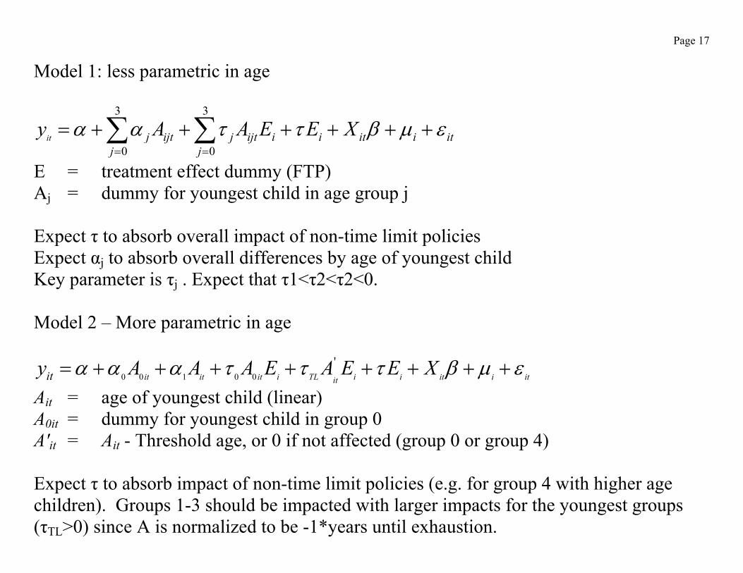
Model 1: less parametric in age

3 3

0 0it j ijt j ijt i i it i it

j jy A A E E Xα α τ τ β μ ε

= =

= + + + + + +∑ ∑

E = treatment effect dummy (FTP) Aj = dummy for youngest child in age group j Expect τ to absorb overall impact of non-time limit policies Expect αj to absorb overall differences by age of youngest child Key parameter is τj . Expect that τ1<τ2<τ2<0. Model 2 – More parametric in age

0 0 1 0 0

'it it it i TL i i it i ititity A A A E A E E Xα α α τ τ τ β μ ε= + + + + + + + +

Ait = age of youngest child (linear) A0it = dummy for youngest child in group 0 A'it = Ait - Threshold age, or 0 if not affected (group 0 or group 4) Expect τ to absorb impact of non-time limit policies (e.g. for group 4 with higher age children). Groups 1-3 should be impacted with larger impacts for the youngest groups (τTL>0) since A is normalized to be -1*years until exhaustion.

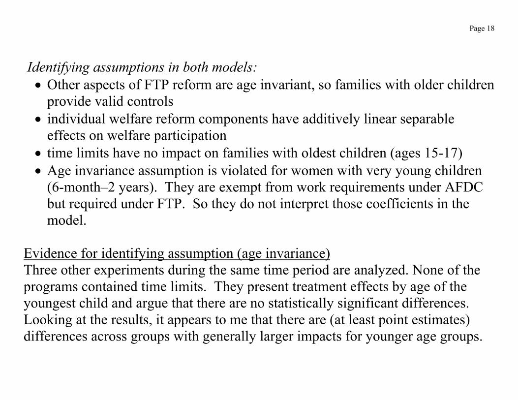
Identifying assumptions in both models: • Other aspects of FTP reform are age invariant, so families with older children

provide valid controls • individual welfare reform components have additively linear separable

effects on welfare participation • time limits have no impact on families with oldest children (ages 15-17) • Age invariance assumption is violated for women with very young children

(6-month–2 years). They are exempt from work requirements under AFDC but required under FTP. So they do not interpret those coefficients in the model.

Evidence for identifying assumption (age invariance) Three other experiments during the same time period are analyzed. None of the programs contained time limits. They present treatment effects by age of the youngest child and argue that there are no statistically significant differences. Looking at the results, it appears to me that there are (at least point estimates) differences across groups with generally larger impacts for younger age groups.

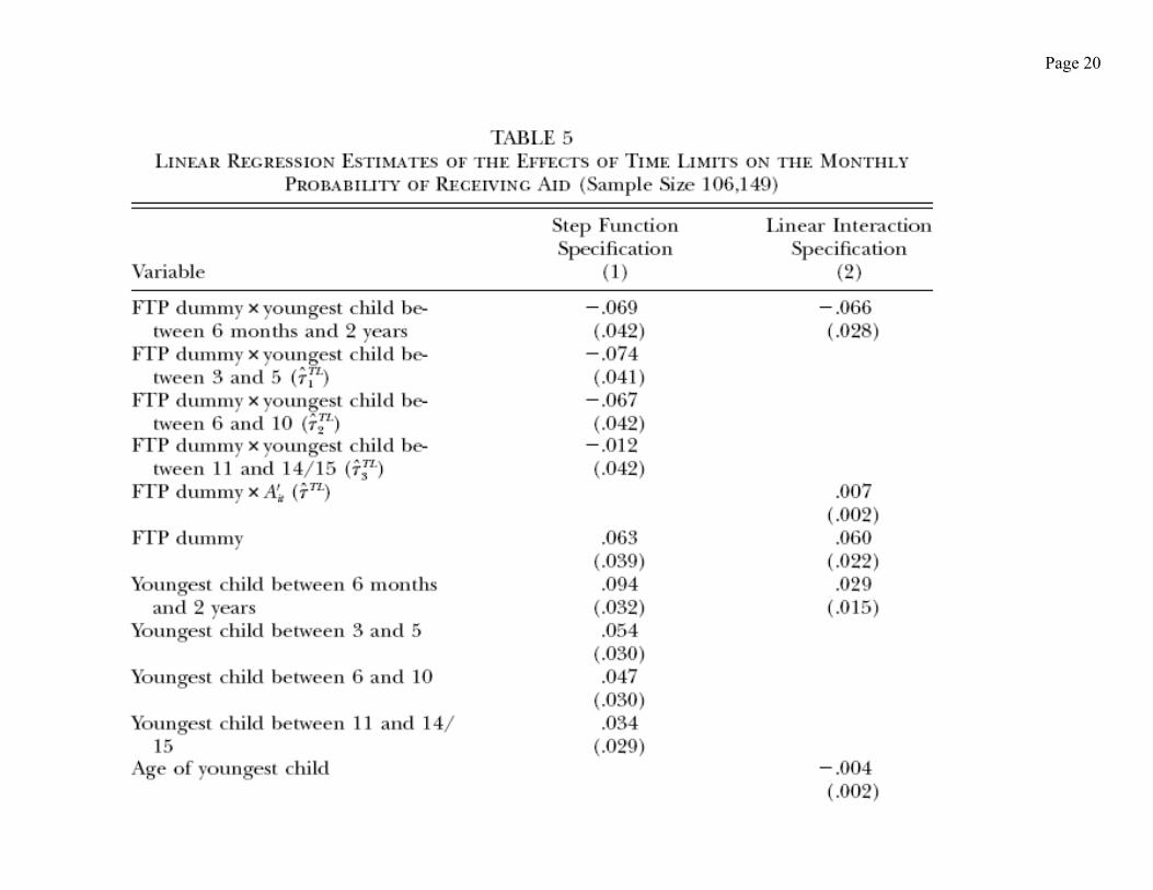
Results: Model 1 estimates in Table 5 (less parametric) • Main effect of FTP (capturing non-TL aspects of reform) is positive,

increasing welfare participation (enhanced earnings disregard) • Marginal impact of TL is negative, with largest impacts for youngest child 6-

10 (relative to older children). Not much difference across age groups 1-2. Model 2 estimates in Table 5 (more parametric) • More precise estimates of TL due to fewer parameters • Again main effect of FTP is positive • Interaction of FTP and time to TL is positive as expected. The younger the

youngest child (the larger negative the A’) and the larger the reduction in welfare participation.

• Magnitude: o 1 year increase in youngest child’s age → 0.7 pp reduction in impact of TL o 36 month TL, 13 yr old → 1.4 pp impact of TL

Critique: • Why not take entire benefit endowment [e.g. keep on welfare until time limit

regardless of child’s age]? You can save the total benefit payment–that will make you better off than conserving it given that benefit is in nominal terms.

• Unobserved heterogeneity in child’s age. Suppose those with older children are the most welfare dependent group. They would be expected to have smaller effects of the policy. Goes in the direction of TL. They address this somewhat by extensions when they estimate models by months on aid before random assignment.

• What if the aspects of the reform are not age invariant? If anything, the results in Table 4 show larger effects of women with the youngest children. So this could bias toward finding a larger impact of time limits given identification strategy. (Literature on EITC shows that the largest impacts were found for women with the youngest children. Differential response to financial incentives?)

• Why not drop youngest children since they face different rules and older children are not a good control group? OR, given that mandatory work requirements should lead to less welfare use, we would expect that the coef on the youngest children would capture impacts of time limits AND new requirements – the implication is that the coef for the youngest group would be larger than for the next youngest group. Why not use that information?

• Why do the unconditional DD results (Table 3 Col 6) not provide the same pattern? If the randomization is done properly, then adding Xs should only improve precision.

In Table 1 they show the Xs are the same in the T and C groups. But they address this by saying that w/in age groups there are differences. So when you control for Xs you get unbiased estimates that are different from DD.

• Table 7 shows estimates where the time period is adjusted. I think it would be useful to show the simple treatment effect by period and how it varies by (age) group. Then you could plot the series for the different age groups. This would show whether the anticipatory behavior starts earlier, later, etc. Maybe not enough obs for this nonparametric estimator.

• The time limit (24 or 36 months) depends on characteristics– more disadvantaged get the 36 month time limit. This enters the regression yet it is endogenous to outcomes. They control for the 24/36 month time limit in the regression but what about the interactions of time limit and age of youngest child? What would happen if they estimate the model separately for each TL group? (Like Table 7 but using another categorizing variable)

• I would like to have a better sense of which age ranges give the variation. The linear assumption imposes this to have a constant impact of 1 year of age. But the step function shows that this can not be valid. I would like to see more richness in the nonparameteric estimator.

• Does it make sense that this population is so forward looking? Jesse Shapiro’s paper on the food stamp program (JPUBE) suggests this is not the case.

A QUICK PRIMER ON EXPERIMENTAL METHODS AND THE EVALUATION PROBLEM

• Evaluation research seeks to estimate the impact of a policy or treatment on an outcome.

• Treatment is dichotomous: received training, faced different welfare program, etc.

• The task of evaluation research, therefore, is to devise methods to reliably estimate their effects on outcomes, so that informed decisions about program expansion and termination can be made.

Treatment effects notation: Yi1 = outcome for i in counterfactual state of receiving treatment Yi0 = outcome for i in counterfactual state of not being treated Di = Treatment indicator [=1 if treated, =0 if not] Treatment effect on i Δi = Yi1 – Yi0 It is the goal of evaluation research to learn about Δi

• The evaluation problem is that the pair (Yi1, Yi0) is never observed. This is true for non-experimental and experimental settings.

• The evaluation problem, therefore, can be considered a missing data problem.

• Most approaches accept the impossibility of constructing Δi and instead seek to estimate the population mean.

MEASURES USED IN EVALUATION LITERATURE Effect of the treatment on the treated E D( | )Δ =1

DEF: Average gain in the outcome for persons in the program– either the group that ‘selects’ into the program, or the group that is (randomly) assigned to the program.

Average treatment effect (ATE) = E(Δ)

DEF: Average gain in the outcome for all persons who are eligible, rather than those who (voluntarily choose to) participate.

Local average treatment effect (LATE)

Generated from some marginal change in the program and/or participants Measures the mean impact of the program on those persons whose participation status changes due to the change in the policy instrument.

(Common effects means that ATE=TT=LATE)

EXPERIMENTAL SOLUTIONS TO EVALUATION PROBLEM • Randomization of program status provides a solution to the problem • Up to sampling variation, the treatment and control groups have the same

distribution of observed and unobserved characteristics • How can we examine the validity of the random assignment assumption?

(check pre RA variables and test for differences btw T and C groups.) Given random assignment, the average effect of treatment on the treated can be estimated by comparing means in the treatment and control groups:

Δ= = − =E Y D E Y D[ | ] [ | ]1 0 How is this estimator compared to the DD estimator? Why is this a single difference estimator? You can also estimate this in a regression framework; and can add covariates to improve efficiency.

“What Mean Impacts Miss: Distributional Impacts of Welfare Reform Experiments” AER 2006 Bitler, Gelbach and Hoynes Purpose of our paper: -- explore heterogeneity in the impact of this treatment -- what can be estimated in experimental context without any further assumptions, maintaining nonparametric appeal of the experimental estimators -- in our application, the theory predicts negative impacts on labor supply for some and positive impacts on labor supply for others. -- Can we reveal these predictions using a nonparametric distributional estimator? We estimate Quantile Treatment Effects (QTEs) • No other assumptions are required beyond random assignment • QTE estimates the impact of the treatment on the distribution of outcomes. • The QTE is analogous to the assumption-free mean impact

Quantile Treatment Effect (QTE) Δq q qy y= −( ) ( )1 0 yq(t) = qth quantile of the marginal distributions (of T and C groups) – QTE for qth quantile is simple difference in quantiles of treatment and control group. – Interpretation: change in expected value of the outcome at the qth quantile when we take a randomly chosen, previously untreated person and give them the treatment. -- given random assignment: the impact of the treatment on the distribution can be estimated without any further assumptions (non-parametric estimator; simple treatment control comparisons) In practice, we have a modest imbalance between the pre-T covariates between the T and C groups. We use inverse propensity score weights when calculating the QTEs (Firpo 2003). We use bootstrap techniques to calculate confidence intervals for each QTE.

Estimators that require more assumptions beyond random assignment: Distribution of Treatment Effects (DTE) Pr(Δi≤δ) ≡ G(δ) DTE gives us measures such as the fraction of losers, Pr(Δi<0) = G(0), or quantiles of treatment effect. But, since we do not observe Δ, we can not make statements about the distribution of Δ without further assumptions. Under some conditions, the QTE tell us about the DTE: – Constant treatment effects – Under rank preservation, QTEs give actual distribution of treatment effects. – If top(bottom) quartile has – (+) QTE, then treatment effect is too.

Argument for usefulness of QTE estimator The estimation of QTEs is sufficient for policy evaluation – Social welfare functions typically rely on marginal distributions (e.g. how does a given policy change the distribution of income?)

Why we use distributional methods in this application • labor supply theory predicts reduction in labor supply for some and increase for

others. Does mean impact estimator reveal these patterns? Can miss the negatives for some and positives for others.

• allows a better “test” of the theory. WHY USE EXPERIMENTAL DATA?

• Want to use an empirical framework where the identification is clear and incontrovertible

• Identification of impacts of welfare reform using nonexperimental methods is less clear; especially for TANF

WHY CONNECTICUT JOBS FIRST PROGRAM?

• Most TANF-like of all programs evaluated using experimental design • The heterogeneous labor supply predictions we predict are not new–-but no previous study has identified this type of behavior • JF has most dramatic change to work incentives that I know of

Validity of the experiment: Things to check (always): 1. Is the treatment assigned randomly: test for differences between observables at random assignment. 2. Is there differential attrition from the experiment between the treatment and control group?

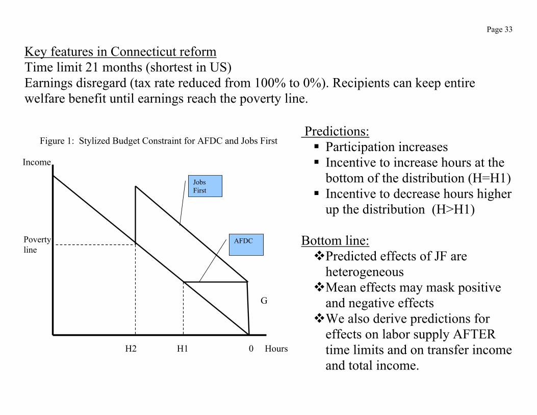
Key features in Connecticut reform Time limit 21 months (shortest in US) Earnings disregard (tax rate reduced from 100% to 0%). Recipients can keep entire welfare benefit until earnings reach the poverty line.

Predictions:

Participation increases Incentive to increase hours at the bottom of the distribution (H=H1)

Incentive to decrease hours higher up the distribution (H>H1)

Bottom line:

Predicted effects of JF are heterogeneous Mean effects may mask positive and negative effects We also derive predictions for effects on labor supply AFTER time limits and on transfer income and total income.

Poverty line

Income

Hours H1 H2

Figure 1: Stylized Budget Constraint for AFDC and Jobs First

0

AFDC

Jobs First

G

EXPERIMENT AND DATA: – Statewide waiver program – Random assignment 1/96-2/97; 4 year followup – Evaluation in New Haven & Manchester – Public use data (MDRC): 4,803 single parent cases – Administrative data on earnings (from UI) and transfer payments (AFDC/JF and Food stamps) – Demographic data from pre-RA interview

Illustrating how to calculate the QTE. Here are the main results for labor supply (earnings) prior to time limits. Consistent with theoretical predictions. Very different from mean

impacts.

Percentile

10 20 30 40 50 60 70 80 90

-1400

-1000

-600

-200

200

600

1000

1400

$0

$1,000

$2,000

$3,000

$4,000

$5,000

$6,000

$7,000

$8,000

10 20 30 40 50 60 70 80 90percentile

Qua

rterly

Ear

ning

s

Jobs First

AFDC

means by group

QTE FOR EARNINGS BEFORE AND AFTER TIME LIMITS.

Figure 3: Quantile Treatment Effects on Distribution of Earnings, Quarters 1-7

-$600

-$400

-$200

$0

$200

$400

$600

$800

$1,000

10 20 30 40 50 60 70 80 90Quantile

Qua

rter

ly Im

pac

Figure 4: Quantile Treatment Effects on Distribution of Earnings, Quarters 8-16

-$600

-$400

-$200

$0

$200

$400

$600

$800

$1,000

10 20 30 40 50 60 70 80 90Quantile

Qua

rter

ly I

mpa

QTE FOR TRANSFERS BEFORE AND AFTER TIME LIMITS.

Figure 6: Quantile Treatment Effects on Distribution of Transfers, Quarters 8-16

-$800

-$600

-$400

-$200

$0

$200

$400

$600

$800

$1,000

10 20 30 40 50 60 70 80 90Quantile

Qua

rter

ly Im

pac

Figure 5: Quantile Treatment Effects on Distribution of Transfers, Quarters 1-7

-$600

-$400

-$200

$0

$200

$400

$600

$800

$1,000

10 20 30 40 50 60 70 80 90Quantile

Qua

rter

ly Im

pac

QTE FOR INCOME BEFORE AND AFTER TIME LIMITS.

Figure 8: Quantile Treatment Effects on Distribution of Income, Quarters 8-16

-$600

-$400

-$200

$0

$200

$400

$600

$800

$1,000

10 20 30 40 50 60 70 80 90Quantile

Qua

rter

ly Im

pac

Figure 7: Quantile Treatment Effects on Distribution of Income, Quarters 1-7

-$600

-$400

-$200

$0

$200

$400

$600

$800

$1,000

10 20 30 40 50 60 70 80 90Quantile

Qua

rter

ly Im

pac

DETAILS: ESTIMATING THE QTE 1. Estimate inverse propensity scores

• Estimate logit with dependent variable equal to treatment dummy Pr[Ti=1] as a function of pre-random assignment variables

• Predict probability for each observation, pi

• Form inverse propensity score weight: wTp

Tp

ii

i

i

i= +

−

−

11

1. Construct quantiles of JF and AFDC distribution for quantiles 1, 2, .. 99.

• Construct F y Y y( ) Pr[ ]≡ ≤ accounting for weights

( ) ( )F y Y yi

i

i≡ ≤∑υ1 where υ is the normalized weight.

• Construct quantiles using this empirical weighted distribution– qth quantile of F is the smallest value yq such that ( )F y qq = .

• QTE = −y JF y AFDCq q( ) ( )

DETAILS: BOOTSTRAPPING THE STANDARD ERRORS

For each replication: I. Resample from sample persons and use the full profile of data for the woman.

This accounts for within-person dependence.

II. Draw 2,381 times from JF distribution and 2,392 times from AFDC distribution (sample size)

III. Calculate QTE in replication sample (using estimated propensity score from real sample)

Repeat 1000 times.

IV. For each QTE (quantiles 1-99), calculate standard errors using empirical standard deviation of the bootstrap sample.

V. Calculate confidence intervals using standard normal distribution.

uc davis ec230 1.overview of welfare reform 2.expected effects of

Documents