u r b health and theb e a report prepared for the leed · pdf filetable 3-7 accident rates by...
TRANSCRIPT

U N D E R S TA N D I N G T H E R E L AT I O N S H I P B E T W E E NP U B L I C H E A LT H A N D T H E B U I LT E N V I RO N M E N T
A REPORT PREPARED FOR THE LEED-ND CORE COMMITTEE
May 2006

PPrreeppaarreedd BByy ::Des ign , Community & Env i ronmentDr. Re id Ewing Lawrence Fr ank and Company, IncDr. R ichard Kreutzer
A REPORT PREPARED FOR THE LEED-ND CORE COMMITTEE
May 2006
U N D E R S TA N D I N G T H E R E L AT I O N S H I P B E T W E E NP U B L I C H E A LT H A N D T H E B U I LT E N V I RO N M E N T

TABLE OF CONTENTS
1. INTRODUCTION .................................................................................. 1 2. RESPIRATORY AND CARDIOVASCULAR HEALTH.................................... 3 3. FATAL AND NON-FATAL INJURIES........................................................ 33 4. PHYSICAL FITNESS............................................................................. 69 5. SOCIAL CAPITAL ................................................................................ 89 6. MENTAL HEALTH................................................................................ 101 7. SPECIAL POPULATIONS ...................................................................... 107 8. SUMMARY CONCLUSIONS ................................................................... 115 9. LIST OF PREPARERS .......................................................................... 131
List of Figures Figure 2-1 Model Linking Built Environment and Health ...................................... 6 Figure 2-2 Hydrocarbon Emissions from a Hypothetical Vehicle Trip ................. 13 Figure 2-3 Growth in VMT and Population (1980 -1987) ....................................... 13 Figure 2-4 Home and Work Tract Densities and Vehicle Emissions..................... 20 Figure 3-1 Average Traffic Fatalities vs. Homicides – Pittsburgh........................... 39 Figure 3-2 Average Lane Widths vs. 85th Percentile Speed...................................... 43 Figure 3-3 Collision Reductions from Traffic Calming Measures........................... 45 Figure 3-4 Effect of Access Spacing on Accident Rates .......................................... 49 Figure 3-5 Pedestrian Crash Rates on Suburban Arterials ...................................... 51 Figure 3-6 Pedestrian Crash Rates vs. Type of Crossing.......................................... 56
List of Tables Table 2-1 Major Air Pollutants .................................................................................... 11 Table 2-2 Growth in Daily VMT and Population 1982-1996.................................. 15 Table 2-3 Travel and Emission Indicators: Infill vs. Greenfield Sites .................... 24 Table 3-1 Most Dangerous Metropolitan Areas for Pedestrians............................. 35 Table 3-2 Traffic Safety Measures for 13 Study Regions.......................................... 38
i

P U B L I C H E A L T H A N D T H E B U I L T E N V I R O N M E N T T A B L E O F C O N T E N T S
Table 3-3 Travel Elasticities of the 3Ds/Regional Accessibility.............................. 40 Table 3-4 Safety Impacts of Traffic Calming ............................................................. 47 Table 3-5 Urban and Suburban Crash Rates by Level of Access Control ............. 48 Table 3-6 Crash Rates at Roundabouts and Signalized Intersections ..................... 53 Table 3-7 Accident Rates by Land Width and Roadside Recovery......................... 55 Table 5-1 Features of Sprawl that Weaken Sense of Community ........................... 94
i i
1 INTRODUCTION
This report presents an appraisal of the current state of the research regarding the links between public health and neighborhood design and provides recommendations about how this knowledge can be integrated into the LEED-ND rating system to improve public health. The report was prepared for the US Green Building Council (USGBC), Congress for the New Urbanism (CNU), the Natural Resources Defense Council (NRDC) and the participants in the Leadership in Energy and Environmental Design for Neighborhood Development (LEED-ND) Core Committee. LEED-ND is a rating system for neighborhood location and design based on the combined principles of smart growth, urbanism, and green building. The purpose of this report is to better understand the specific development patterns and changes to the built environment will have a significant impact on public health. The report is comprised of nine chapters, including this introduction. Apart from this first chapter and the chapter on special populations, the research findings sections are primarily organized by major health outcomes. The summary conclusions, on the other hand, are organized by characteristics of urban form that can be addressed in the LEED-ND rating system. The chapters include:
♦ The Introduction explains the purpose of the report and provides an overview the contents. It also includes a section briefly introducing a discussion about how the urban form is measured. This discussion is carried on throughout the remaining chapters.
♦ Respiratory and Cardiovascular Health introduces the concept of the land use and transportation connection as part of a discussion about how the urban environment impacts vehicle travel and emissions. Once this link is established, the chapter discusses the link between vehicle emissions, air quality and respiratory and cardiovascular health.
♦ Fatal and Non-fatal Injuries, written by Dr. Reid Ewing, presents extensive information about links between roadway and network design, traffic calming and other aspects of transportation with incidents of injuries.
♦ Physical Fitness presents evidence about the growing health epidemic related to physical inactivity and the relationship that research has shown between rates of walking, bicycling and transit use and the built environment.
♦ Social Capital describes the benefits that accrue from healthy social networks and how the built environment may help or impair the formation and sustenance of those systems.
1
P U B L I C H E A L T H A N D T H E B U I L T E N V I R O N M E N T I N T R O D U C T I O N
♦ Mental Health presents what little is known about the links between urban form and mental health issues including overall mental health, depression, stress, aggressive driving and road rage.
♦ Special Populations discusses the disproportionate impacts that poor public transportation, inadequate pedestrian environments and car dependent environments have on subgroups in America including women, children, low income communities, the elderly and persons with disabilities.
♦ Summary Conclusions summarizes the findings from the previous chapters in terms of characteristics of the built environment that can be affected by developers to provide maximum public health benefits.
♦ List of Preparers lists the consultant team who researched and wrote the report and acknowledges the reviewers and funders of the study.
2

2 RESPIRATORY AND CARDIOVASCULAR HEALTH
The research on respiratory and cardiovascular function, shows a link between the built environment and health. Studies demonstrate the connection by methodically moving through a series of connections beginning with the built environment and ending with cardiovascular and respiratory health. The first correlation that is established in the literature is that the compactness of land uses and the organization of the transportation system determines, to a large extent, how much individuals drive. The more sprawling and disconnected houses are from workplaces and shops, the more miles and hours individuals must travel to get from one place to another. If there are no reasonably convenient or affordable alternatives to driving then all of those hours traveling will be spent behind the wheel of a car.1 Once it has been established that the organization of the built environment affects travel, both in the form of vehicle trip generation rates and distances traveled, the link to air pollution and respiratory health becomes easier to see. There is extensive research showing that driving is a major source of air pollution. Vehicle emissions are most often measured at two points during a vehicle trip: when a car is turned on (cold-starts) and over the distances traveled once an engine has warmed up (hot-stabilized emissions). Cold-starts are measured because they are highly polluting. However, researchers have shown that vehicles continue to pollute once they have warmed up, which can be particularly problematic in sprawling environments where vehicles have to travel in congested conditions.2,3 The pollutants that have been attributed to vehicle travel include carbon monoxide (CO), particulate matter (PM), and other air toxins, which are harmful in their own right; as well as nitrogen oxides (NOx) and volatile organic compounds (VOC), which combine to form ozone.2-5 Research shows that both cold-start and hot stabilized emissions generated per capita are related to the design of the built environment.4 The more times cars are
1 Frank, Lawrence D., Engelke, Peter and Schmid, Tom. Health and Community
Design: The Impacts of the Built Environment on Physical Activity, Island Press – Spring 2003.
2 Frumkin, Howard, Lawrence Frank and Richard Jackson. Urban Sprawl and Public Health. Island Press 2004.
3 Ewing, R. & Cervero, R. (2001). The influence of land use on travel behavior: Empirical strategies. Transportation Research, Policy and Practice, 35, 823-845.
4 Frank, Lawrence, Brian Stone Jr., and William Bachman. 2000. Linking Land Use with Household Vehicle Emissions in the Central Puget Sound: Methodological Framework and Findings. Transportation Research Part D 5, 3: 173-96.
3

P U B L I C H E A L T H A N D T H E B U I L T E N V I R O N M E N T R E S P I R A T O R Y A N D C A R D I O V A S C U L A R H E A L T H
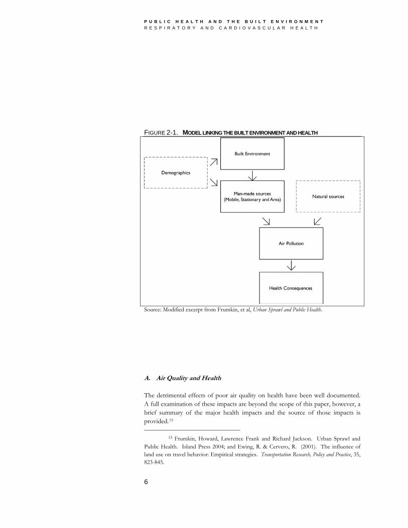
started, miles are traveled and hours are spent idling in traffic, the more emissions are released.5 Spreading houses, jobs, and shops further apart and limiting alternative modes of travel ultimately increases the need for cars to get to all of these locations, which in turn increases air pollution. While considerably strengthened in recent years,6 the link between air pollution and respiratory health was established years ago.7 Breathing higher concentrations of CO, VOC, fine particulate matter (< 2.5 microns) and other emissions released from tail pipes has consistently been shown to induce detrimental health outcomes. More specifically, concentrations of ozone in excess of 80 parts per billion sustained over an 8 hour period has been found to reduce lung capacity, increase instances of severe asthma, and in certain cases, impact life expectancy.8,9 ,10 Recent evidence also shows how increased exposure to fine particulate matter can trigger heart attacks amongst the elderly and other at risk populations.11 The evidence for the links between the built environment and health will be discussed in detail in the next section. However, the model shown in Figure 2-1, illustrates the links just described with the addition of two factors: demographics
5 Frank, Lawrence and Engelke, Peter. In Press. “Multiple Impacts Of The Built
Environment On Public Health: Walkable Places And the Exposure To Air Pollution.” International Regional Science Review.
6 Bell, M.L., McDermott, A., Zeger, S., Samet, JM, Dominici, F. 2004. Ozone and Short-Term Mortality in 95 U.S. Urban Communities, 1987-2000. New England Journal of Medicine.
7 Frumkin, Howard, Lawrence Frank and Richard Jackson. Urban Sprawl and Public Health. Island Press 2004; and Ewing, R. & Cervero, R. (2001). The influence of land use on travel behavior: Empirical strategies. Transportation Research, Policy and Practice, 35, 823-845.
8 US Environmental Protection Agency. National Emission Standards for Hazardous Air Pollutants, 2003. 40 Cfr Parts 50, 51 and 81.
9 Hoek, Gerard, Bert Brunekreef, Sandra Goldbohm, Paul Fischer, and Piet A. van den Brandt. 2002. Association between mortality and indicators of traffic-related air pollution in the Netherlands: A cohort study. Lancet 360: 1203-9.
10 Friedman, M., K. Powell, L. Hutwagner, L. Graham, and W. Teague. 1998. Impact of changes in transportation and commuting behaviors during the 1996 Summer Olympic Games in Atlanta on air quality and childhood asthma. Journal of the American Medical Association 285, 7: 897-905.
11 Pope, C., R. Burnett, M. Thun, E. Calle, D. Krewski, K. Ito, and G. Thurston. 2000. Lung cancer, cardiopulmonary mortality, and long-term exposure to fine particulate air pollution. Journal of the American Medical Association 287: 1132-41.
4

P U B L I C H E A L T H A N D T H E B U I L T E N V I R O N M E N T R E S P I R A T O R Y A N D C A R D I O V A S C U L A R H E A L T H
and natural sources of air pollution. Demographic factors, such as income, age, gender, ethnicity and household structure contribute to individual decisions about how many trips to take, where to go and how to get there.12 When measuring the magnitude of the impact of the built environment on travel choices, it is necessary to control for these individual characteristics and, to the extent possible, preferences to accurately understand the dynamics between urban form and travel. Secondly, Figure 2-1 shows two sources of air pollution: man-made sources and natural sources. Natural sources of air pollution are all around us. Pollutants are released from many natural features including oceans, vegetation, forest fires, and wind across dusty landscapes. Pollution from these natural sources include volatile organic compounds (hydro-carbons) and create a background of pollution against which man-made emissions must be separated and measured. For example, pollution from man-made sources such as NOx can interact with natural sources of VOCs to worsen air quality and thus increase health impacts. Thus, studies show that the amount of vehicular travel, both in the number of trips and in the miles traveled, is affected by the design of the built environment and that this travel impacts how much air pollution we each generate. Finally, research shows that many of the resulting pollutants are bad for health. Therefore, through a series of relationships it becomes clear that the form of the built environment is indeed linked to public health. Development patterns can have negative affects on air quality as when sprawling land uses, such as large lots and disconnected street networks, encourage driving.13 Controlling the spread of development can reduce distances and associated emissions on a per capita basis as can significant advances in technologies to reduce emissions on a per miles basis. However, these gains are offset by the ever increasing number of drivers on the road resulting from population growth worldwide.14
12 Adler, T. J. and Ben-Aldva, M. E., (1979), “A theoretical and empirical model of
trip chaining behavior,” Transportation Research, 13B 13 Frank, L.D., Sallis, J.F., Wolf, K., Piro, R., Linton, L. Submitted. Zoning for
Health: The Physical Activity, Obesity, and Respiratory Impacts of Land Use Regulation.” Journal of the American Planning Association.
14 Transit Cooperative Research Program, The Costs of Sprawl – Revisited - Literature Synthesis. Transportation Research Board, August 31, 2001, pages 62-66.
5
P U B L I C H E A L T H A N D T H E B U I L T E N V I R O N M E N T R E S P I R A T O R Y A N D C A R D I O V A S C U L A R H E A L T H
FIGURE 2-1. MODEL LINKING THE BUILT ENVIRONMENT AND HEALTH
Source: Modified excerpt from Frumkin, et al, Urban Sprawl and Public Health. A. Air Quality and Health The detrimental effects of poor air quality on health have been well documented. A full examination of these impacts are beyond the scope of this paper, however, a brief summary of the major health impacts and the source of those impacts is provided.15
15 Frumkin, Howard, Lawrence Frank and Richard Jackson. Urban Sprawl and
Public Health. Island Press 2004; and Ewing, R. & Cervero, R. (2001). The influence of land use on travel behavior: Empirical strategies. Transportation Research, Policy and Practice, 35, 823-845.
6

P U B L I C H E A L T H A N D T H E B U I L T E N V I R O N M E N T R E S P I R A T O R Y A N D C A R D I O V A S C U L A R H E A L T H
The importance of the link between air quality and health was first acknowledged nationally in the Clean Air Act of 1970 and has been the on-going subject of research and policy interventions. Air pollution is related to four major health threats: increased mortality, respiratory illnesses, impaired cardiovascular functions and increased cancer risk.16 Researchers continue to find new health threats and improve the understanding of the mechanisms that bring toxins into the air.17 1. Mortality The first hypotheses that air quality was linked to increased death rates arose in the early part of the 20th century. There were several severe air pollution events during the first fifty years of the century that coincided with increased mortality rates. However, it wasn’t until the 1950s, that scientists began extensively studying the phenomenon and made the link between pollution thick with particulate matter (PM) and Sulfur Oxides (SOx) and increased death rates.18 Recent research has confirmed these early results and contributed additional information showing that even the current amount of PM in the air is responsible for loss of life. One study in Ohio compared death rates in six cities with differing PM levels over 10 years. Researchers found that residents of city with the highest PM levels had death rates that were 26 percent higher than those in the city with the lowest levels, while the other cities fell in between.19 Another study done in Europe showed that 10 μg/m3 increase in the concentration of PM10 would result in a 0.6 to 0.7 increase in mortality rates. Rates increased with higher NOx pollution, with elderly people and in warm and dry climates.20 Similar results have been found in the U.S. While this percentage may seem small, the Natural Resources Defense Council has estimated that approximately 64,000 people die
16 Frumkin, Howard, Lawrence Frank and Richard Jackson. Urban Sprawl and
Public Health. Island Press 2004. 17 Schauer, James, Wolfgang Rogge, Lynn Hildemann, Monica Mazurek, Glen
Cass, and Bernd Simoneit. 1996. Source appointment of airborne particulate matter using organic compounds as tracers. Atmospheric Environment 30, 22: 3837-55.
18 Frumkin, Howard, Lawrence Frank and Richard Jackson. Urban Sprawl and Public Health. Island Press 2004.
19 Bell, M.L., McDermott, A., Zeger, S., Samet, JM, Dominici, F. “2004. Ozone and Short-Term Mortality in 95 U.S. Urban Communities, 1987-2000.” New England Journal of Medicine.
20 Katsouyanni, K and Pershagen, G. “Ambient Air Pollution Exposure and Cancer,” Cancer Causes and Controls Vol 8 Issue 3 pages 284-91; 1997.
7
P U B L I C H E A L T H A N D T H E B U I L T E N V I R O N M E N T R E S P I R A T O R Y A N D C A R D I O V A S C U L A R H E A L T H
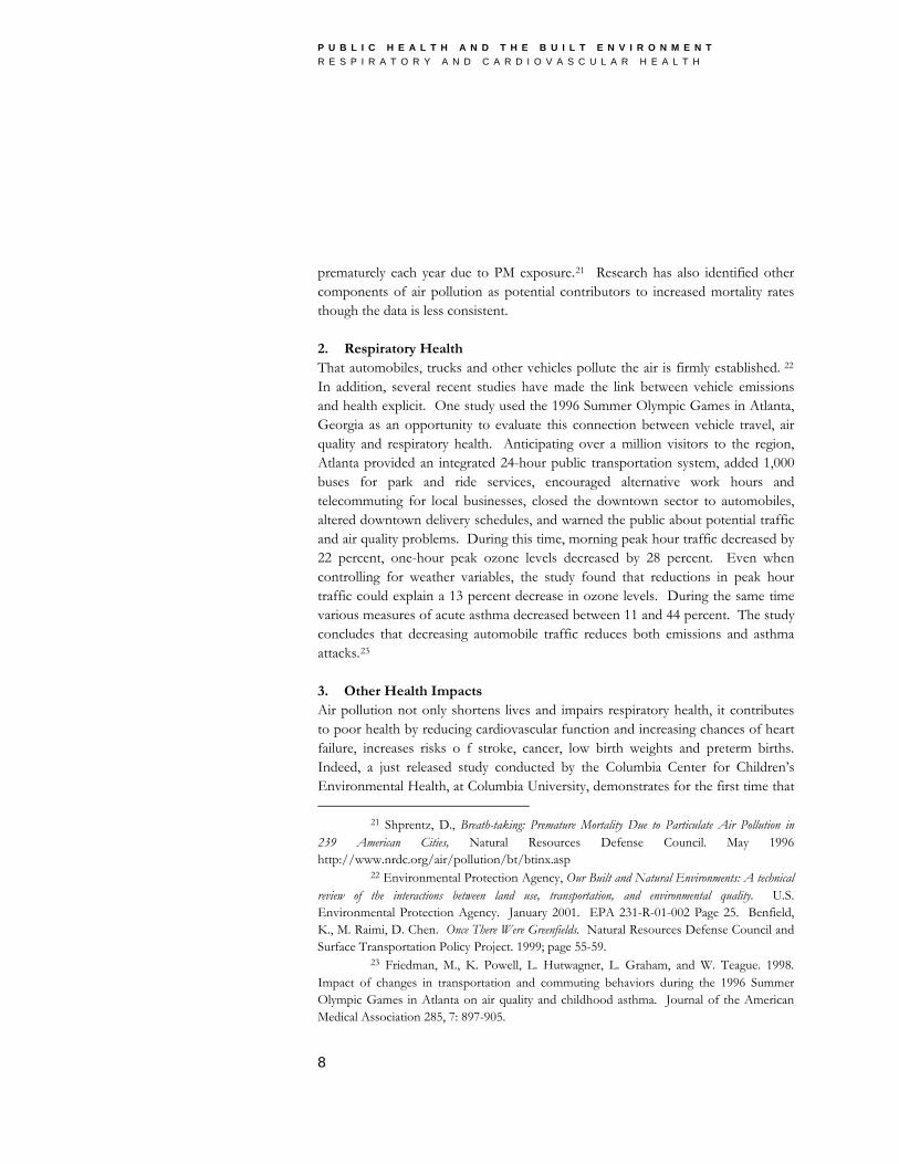
prematurely each year due to PM exposure.21 Research has also identified other components of air pollution as potential contributors to increased mortality rates though the data is less consistent. 2. Respiratory Health That automobiles, trucks and other vehicles pollute the air is firmly established. 22 In addition, several recent studies have made the link between vehicle emissions and health explicit. One study used the 1996 Summer Olympic Games in Atlanta, Georgia as an opportunity to evaluate this connection between vehicle travel, air quality and respiratory health. Anticipating over a million visitors to the region, Atlanta provided an integrated 24-hour public transportation system, added 1,000 buses for park and ride services, encouraged alternative work hours and telecommuting for local businesses, closed the downtown sector to automobiles, altered downtown delivery schedules, and warned the public about potential traffic and air quality problems. During this time, morning peak hour traffic decreased by 22 percent, one-hour peak ozone levels decreased by 28 percent. Even when controlling for weather variables, the study found that reductions in peak hour traffic could explain a 13 percent decrease in ozone levels. During the same time various measures of acute asthma decreased between 11 and 44 percent. The study concludes that decreasing automobile traffic reduces both emissions and asthma attacks.23
3. Other Health Impacts Air pollution not only shortens lives and impairs respiratory health, it contributes to poor health by reducing cardiovascular function and increasing chances of heart failure, increases risks o f stroke, cancer, low birth weights and preterm births. Indeed, a just released study conducted by the Columbia Center for Children’s Environmental Health, at Columbia University, demonstrates for the first time that
21 Shprentz, D., Breath-taking: Premature Mortality Due to Particulate Air Pollution in 239 American Cities, Natural Resources Defense Council. May 1996 http://www.nrdc.org/air/pollution/bt/btinx.asp
22 Environmental Protection Agency, Our Built and Natural Environments: A technical review of the interactions between land use, transportation, and environmental quality. U.S. Environmental Protection Agency. January 2001. EPA 231-R-01-002 Page 25. Benfield, K., M. Raimi, D. Chen. Once There Were Greenfields. Natural Resources Defense Council and Surface Transportation Policy Project. 1999; page 55-59.
23 Friedman, M., K. Powell, L. Hutwagner, L. Graham, and W. Teague. 1998. Impact of changes in transportation and commuting behaviors during the 1996 Summer Olympic Games in Atlanta on air quality and childhood asthma. Journal of the American Medical Association 285, 7: 897-905.
8

P U B L I C H E A L T H A N D T H E B U I L T E N V I R O N M E N T R E S P I R A T O R Y A N D C A R D I O V A S C U L A R H E A L T H
prenatal exposure to airborne hydrocarbons may cause chromosomal aberrations and increase cancer risk in newborns.24
B. Sources of Air Pollution Air pollution is not one single substance. It is made up of numerous compounds and particles that are released from different sources.25 The independent components of air pollution which are generally measured include:
♦ Carbon Monoxide (CO) ♦ Sulfur Oxides (SOx) ♦ Nitrogen Oxides (NOx) ♦ Particulate Matter (PM10 and PM2.5) ♦ Ozone ♦ Lead ♦ Volatile Organic Compounds (VOCs) ♦ Air Toxics (e.g. benzene, formaldehyde, methanol, etc.) ♦ Carbon Dioxide (CO2)
Air pollution comes from both man-made and natural sources and varies substantially from place to place based on local weather patterns and resulting vegetative cover. Natural sources are not discussed in this paper. Man-made air pollutants come from three sources: stationary, area and mobile. 1. Stationary and Area Sources Stationary, or point, sources are well-documented contributors to poor air quality and include power plants and factories. Area sources encompass a combination of land uses, such as airports, agricultural feedlots and unpaved roads, and small items that are used on specific sites such as fireplaces and lawnmowers. Area sources also include polluting events such as forest fires.
24 Bocskay, Kirsti A., et al.. Chromosomal Aberrations in Cord Blood are Associated with Prenatal Exposure to Carcinogenic Polycyclic Aromatic Hydrocarbons” Columbia Center for Children’s Environmental Health, Mailman School of Public Health, Columbia University, New York, NY, USA. Study results will be published in Cancer Epidemiology Biomarkers and Prevention.
25 Schauer, J., et al, “Source appointment of airborne particulate matter using organic compounds as tracers”, Atmospheric Environment Vol. 30 Iss. 22, 1996, pages 3837-55.
9
P U B L I C H E A L T H A N D T H E B U I L T E N V I R O N M E N T R E S P I R A T O R Y A N D C A R D I O V A S C U L A R H E A L T H
Land use and zoning policies determine the location, quantity and distribution of stationary sources by regulating their location often to industrial corridors away from population centers. Stationary sources have also been the subject of federal regulations since the passage of the Clean Air Act in 1970. For area sources, land development regulations sometimes determine location, for uses such as airports and feedlots. For smaller polluters, lot size regulations have a greater impact as they determine the types of houses that are built and amenities that will be used to maintain them. Large lots, as are common in many new subdivisions, generally encourage large lawns, which increase the use of lawnmowers, and internal amenities like fireplaces. 2. Mobile Sources Mobile sources, which include cars, trucks and off-road equipment such as bulldozers, trains, boats and airplanes, are also an important contributor to air pollution. As with stationary and area sources, land use and zoning regulations impact the distribution, quantity and exposure people have to these sources. However, the mechanism by which these land development regulations interact with mobile sources is much more complex and will be discussed in detail in the next section. For the moment, it is important to understand the impact mobile sources have on air quality. Statistics collected by the EPA show that alone, cars and trucks account for a considerable portion of the major air pollutants in the United States. As Table 2-1 shows, more than three quarters of CO pollution in the atmosphere comes from cars, trucks and buses. While mobile sources contribute most to CO pollution, they also contribute more than half of the NOx, nearly half the VOCs, and almost a third of carbon dioxide CO2 and other air toxins such as benzene and formaldehyde, all hazardous to human health. In addition, CO2 contributes the most to human-induced global warming of the CO2 the six greenhouse gases normally targeted, according to the Pew Center on Global Climate Change.26 The statistics shown in the table are national averages, however, in areas with heavy traffic and little industry, the percentage of air pollution from mobile sources is much higher.
26 http://www.pewclimate.org/global-warming-basics/facts_and_figures/index.cfm
accessed on April 14, 2005.
10

P U B L I C H E A L T H A N D T H E B U I L T E N V I R O N M E N T R E S P I R A T O R Y A N D C A R D I O V A S C U L A R H E A L T H
TABLE 2-1 Major Air Pollutants, United States 1999
Pollutant Contribution of Cars and Trucks1
Carbon Monoxide (CO) 77%
Sulfur Oxides (Sox) 7%
Nitrogen Oxides (NOx) 56%
Particulate Matter (PM10) 25%2
Particulate Matter (PM2.5) 28%2
Ozone N/A
Lead 13%
Volatile Organic Compounds (VOCs) 47%
Air Toxics (e.g. benzene, formaldehyde, methanol, etc.) 31%
Carbon Dioxide (CO2) 30%
1. Proportions refer to man-made sources only. In some cases, natural sources account for a substantial portion of total contributions. 2. The figure refers only to directly emitted particulate matter. The true contribution of cars and trucks to PM levels is higher than 19%,l since other pollutants, such as NOx and hydrocarbons combine to form PM in the atmosphere after they are released. Sources: Table 2-1 is adapted from Urban Sprawl and Public Health by Howard Frumkin, Lawrence Frank and Richard Jackson. Data represented comes from EPA documents: National Air Quality Emissions Trend Report, 1999 (EPA-454/R-01-004), Toxic Air Pollutants and “The Projection of Mobile Source Air Toxics from 1996 to 2007”: Emissions and Concentrations” (EPA-420/R-01-038), and National Air Pollutant Emission Trends: 1900-1998 (EPA-454/R-00-002).
3. How Vehicles Pollute The quantity and composition of air pollution from mobile sources in a particular area is the function of four variables: the types and length of trips people take in their cars, the types of vehicles they have, the characteristics of the particular pollutants in the area and weather conditions. Only trip characteristics will be discussed in this section, as they are the most closely linked to the built environment.
11

P U B L I C H E A L T H A N D T H E B U I L T E N V I R O N M E N T R E S P I R A T O R Y A N D C A R D I O V A S C U L A R H E A L T H
Vehicles emit different types of pollutants based on their average speed, the length of the trip (VMT), and the duration of the trip (VHT). Vehicle speed, VMT, and VHT are determined, at least in part, by aspects of the built environment. For instance, the potential speed of traffic is primarily determined by the design of a roadway. Roads with wide lanes, few obstacles and limited access allow drivers to attain high speeds whereas narrow lanes with limited range of sight and parking along the sides require drivers to slow down. As previously noted, the distance and time of travel is partly determined by how far apart uses are located. Starting a vehicle engine that has cooled off for more than one hour, is known as a “cold start,” and is the single most polluting portion of every trip, accounting for over 50 percent of CO and VOC emissions, according to one study.27 Acceleration, going uphill and turning a vehicle off are also major points at which emission rates are at their highest. The pattern of emissions during a hypothetical vehicle trip was mapped by Bachman et al, at least for some gases, as is shown in Figure 2-2. If turning on and turning off a vehicle is, in itself, significantly polluting, it is clear that minimizing the total number of vehicle trips is a key step to reducing emissions. Other key conclusions are that reducing VMT, VHT and congestion are all important steps to improving air quality. C. Linking the Built Environment and Travel Behavior In recent decades, VMT has increased at three times the rate of population growth. VMT has similarly outpaced employment and economic growth. This trend is illustrated in Figure 2-3, which shows the growth in vehicle miles traveled compared to the rate of increase in population between 1980 and 1997.28 The increase in VMT is particularly marked in the fastest growing regions of the country. These regions have featured more road building and greater expansion into exurban areas as well as the fastest growth in automobile travel.
27 Frank L., B. Stone Jr., and W. Bachman. Linking land use with household
vehicle emissions in the central Puget Sound: Methodological framework and findings. Transportation Research Part D 2000; 5(3):173-96.
28 Environmental Protection Agency, Our Built and Natural Environments: A technical review of the interactions between land use, transportation, and environmental quality. U.S. Environmental Protection Agency. January 2001. EPA 231-R-01-002 Pages 19-20.
12

P U B L I C H E A L T H A N D T H E B U I L T E N V I R O N M E N T R E S P I R A T O R Y A N D C A R D I O V A S C U L A R H E A L T H
FIGURE 2-2. HYDROCARBON EMISSIONS FROM A HYPOTHETICAL VEHICLE TRIP
Source: Bachman, W. J. Grannell, R. Guensler and J. Leonard, “Research Needs in Determining Spatially Resolved Subfleet Characteristics” Transportation Research Record Vol. 1625, 1998 pages 139-46 as excerpted from Frumkin, Howard, Lawrence Frank and Richard Jackson, Urban Sprawl and Public Health. Island Press 2004. FIGURE 2-3 GROWTH IN VEHICLE MILES TRAVELED & POPULATION (1980-1997)
Sources: U.S. Department of Transportation, Federal Highway Administration. Highway Statistics (Summary to 1995, and annual editions, 1996 and 1997), Washington, and Environmental Protection Agency, Our Built and Natural Environment.
13

P U B L I C H E A L T H A N D T H E B U I L T E N V I R O N M E N T R E S P I R A T O R Y A N D C A R D I O V A S C U L A R H E A L T H
From 1960 to 1990, the percentage of workers with jobs outside their counties of residence increased by 200 percent. Such increases in the distance between work and home have contributed to the acceleration of growth in VMT and congestion.29 According to the Sierra Club, the average American driver spends 443 hours, the equivalent of 11 work weeks, in their car a year. Residents of the fastest growing cities have seen faster growth in time spent driving than those with less growth. According to the Texas Transportation Institute (TTI), the annual time drivers spent delayed was 16 hours in 1982. By 2003, that number had risen to 47 hours. Total hours of delay have increased from 0.7 billion hours to 3.7 billion hours over the same time period. TTI has shown that the increases in congestion is occurring in cities of all sizes. In 1982, 70 percent of the areas of the country experienced uncongested traffic conditions, while only 5 percent experienced extreme delays. Today, only 33 percent of the nation’s areas have uncongested traffic conditions and 20 percent have extremely high delays. The remaining 47 percent of places experience delays ranging from moderate to severe.30
Table 2-2 shows the growth rate in daily VMT exceeds population growth in each of the fifteen cities measured. In cities with particularly high population growth, such as Atlanta and Charlotte, VMT growth is particularly high.31 In January 2001, the EPA released Our Built and Natural Environments, a special report that summarized the research linking the built environment to a number of environmental impacts including air quality. The report attributes the growth of VMT to three factors:
29Frumkin, Howard, Lawrence Frank, and Richard Jackson. Urban Sprawl and
Public Health. Island Press 2004. page 9. 30 Schrank, D. and T. Lomax, The 2005 Urban Mobility Report, Texas
Transportation Institute. May 2005. 31 TTI no longer tracks VMT growth per population. Current statistics show that
VMT continues to increase but don’t show how these increases relate to population growth.
14

P U B L I C H E A L T H A N D T H E B U I L T E N V I R O N M E N T R E S P I R A T O R Y A N D C A R D I O V A S C U L A R H E A L T H
TABLE 2-2 DAILY VMT GROWTH EXCEEDS POPULATION GROWTH (1982-1996)
Urbanized Area Population Growth 1982-96
VMT Growth on Freeways and Principal Arterials 1982-96
Atlanta, GA 53% 119%
Boston, MA 6% 31%
Charlotte, NC 63% 105%
Chicago, IL-IN 11%2 79%
Houston, TX 28%2 54%
Kansas City, MO-KS 23% 79%
Miami-Hialeah, FL 18% 61%
Nashville, TN 25% 120%
New York, NY-NJ 3% 40%
Pittsburgh, PA 7% 54%
Portland-Vancouver, OR-WA 26% 98%
Salt Lake City, UT 32% 129%
San Antonio, TX 29% 77%
Seattle-Everett, WA 35% 59%
Washington, DC-MD-VA 28% 78%
Sources: Table is excerpted from Environmental Protection Agency, Our Built and Natural Environments: A technical review of the interactions between land use, transportation, and environmental quality. U.S. Environmental Protection Agency. January 2001. EPA 231-R-01-002 Page 20 and Texas Transportation Institute, Urban Roadway Congestion, Annual Report 1998. Tables A-6 and A-7.
♦ Demographic and market changes that allow more families to own multiple cars and lead more individuals to drive on a regular basis.
♦ Development patterns that lead to increases in the number and average distance of trips.
15
P U B L I C H E A L T H A N D T H E B U I L T E N V I R O N M E N T R E S P I R A T O R Y A N D C A R D I O V A S C U L A R H E A L T H
♦ The ability of increased road capacity to encourage additional travel—“induced travel.
Demographic and market changes account for approximately 36 percent of VMT growth, while the remaining 64 percent can be attributed to land use changes that have increase average trip distances (38 percent of the growth) and the number of trips made (25 percent of the growth). Induced traffic is a term used to describe traffic growth resulting from reductions in the cost of automobile travel. This generally results from increasing highway and other road capacity. In addition to the short-term impact of increasing vehicle trips because of improved traffic conditions, additional road capacity also induces long-term traffic growth by encouraging more dispersed land use patterns, thus increasing trip distance. Growth in VMT attributable to induced traffic is measured under changes to land use. 32
1. Land use patterns There are many studies linking travel behavior and the built environment. These studies generally combine several factors in their analyses including: density, access to transit, pedestrian amenities, allocation of jobs and housing and regional location. In a survey of over 50 studies, Ewing and Cervero found that the built environment does not affect all aspects of travel equally.33 As described in the previous chapter, their review showed that the built environment had the most impact on trip length, VMTs and VHTs. The number of trips taken by an individual, on the other hand, is more correlated with an individual’s socio-economic status than by the features of surrounding neighborhoods. Mode choice is determined by a combination of factors of the built environment and individual characteristics.34 Given that these factors are often studied together it is difficult to pinpoint which specific elements are the most important to creating the observed changes in VMT. However some clear findings can be made. a. Density The density, or compactness, of development has an impact on the amount that people drive and by extension on air pollution in three main ways: it reduces trip
32 Environmental Protection Agency, Our Built and Natural Environments: A technical
review of the interactions between land use, transportation, and environmental quality. U.S. Environmental Protection Agency. January 2001. EPA 231-R-01-002 Page 45.
33 Ewing, R. Cervero, R. Travel and the built environment: a synthesis. Transportation Research Record 1780 2001;87-122.
34 Frumkin et al. Urban Sprawl and Public Health Chapter 1.
16
P U B L I C H E A L T H A N D T H E B U I L T E N V I R O N M E N T R E S P I R A T O R Y A N D C A R D I O V A S C U L A R H E A L T H
lengths, increases mode choice and decreases the need for vehicle ownership.35 In 1994, Holtzclaw compared 28 neighborhoods across northern California and found that a doubling of density yielded up to 30 percent fewer VMTs when higher density was accompanied by high transit service, a mixture of land uses and pedestrian amenities. In a follow-up study published in 2000, Holtzclaw and others studied transportation analysis areas (TAZs) in San Francisco, Chicago and Los Angeles to further determine the effects of residential density and several other key factors in a TAZ on VMT and vehicle ownership. The researchers confirmed earlier findings that doubling residential density can reduce VMT. In this study, in fact the impact of density increases were higher: the results showed that a doubling of density in in Chicago, Los Angeles and San Francisco resulted in a decrease of 32 percent, 35 percent and 43 percent, respectively. Researchers found similar declines in vehicle ownership. An even more interesting findings that resulted from this study, is the fact that Holtzclaw et al developed an equation, based on variations in residential and overall density, transit accessibility, average household size and average household income, that could be scaled to calculate changes in VMT in all three cities with a statistically significant degree of accuracy. This suggests that, within certain regional parameters, these four variables consistently affect the amount that people drive and how many cars they own.36
Another such study, by Lawrence Frank, Brian Stone Jr. and William Bachman, measured the relationship between household and employment density, land use mix, street connectivity and commute length to household vehicle emissions for CO, NOx and VOC. In a straight data analysis, the researchers found that emissions of all three pollutants consistently decreased as household density increased. In particular, emissions decreased at an accelerated rate as workplace density increases. Finally, they found that for individuals with the longest
35 Environmental Protection Agency, Our Built and Natural Environments: A technical
review of the interactions between land use, transportation, and environmental quality. U.S. Environmental Protection Agency. January 2001. EPA 231-R-01-002 Page 44. Frumkin et al, Page 7. Dunphy and Fisher 1994. Frank and Pivo, 1994. Frank, Lawrence D., Brian Stone Jr., William Bachman. “ Linking Land Use with Household Vehicle Emissions in the Central Puget Sound: Methodological Framework and Findings”. Transportation Research Part D 5;2000:173-196.
36Holtzclaw, J. et al, “Location Efficiency: Neighborhood and Socio Economic Characteristics Determine Auto Ownership and Use – Studies in Chicago, Los Angeles and San Francisco”, Transportation Planning and Technology, Vol. 25, 2002, page 1-27..
17

P U B L I C H E A L T H A N D T H E B U I L T E N V I R O N M E N T R E S P I R A T O R Y A N D C A R D I O V A S C U L A R H E A L T H
commutes vehicle emissions increase as distance to work increases, even when they account for reductions in other trips. 37 Frank et al also conducted a regression analysis to control for demographic characteristics of neighborhoods. Results from the regression analysis also clearly illustrate a significant link between density and household vehicle emissions. Household and work place densities were found to have a significant, negative correlation with emissions. That is as densities increase emissions decline. Work place densities were found to have a particularly strong correlation with changes in VMT. Commute distances continued to have a positive correlation with emissions in the regression analysis. Frank’s research and other similar studies show that the relationship of vehicle miles traveled to density is not a linear function. In the most rural areas, where density is lowest, a study by Dunphy and Fisher (Dunphy and Fisher 1994) showed that even significant increases in density have little impact on VMT. However, as density approaches the levels of older suburbs, VMT, VHT and trip lengths go down significantly.38 As illustrated in Figure 2-4, Frank et al and earlier research by Frank and Pivo show that the relationships of VMT, VHT and emissions are correlated with density by functions that have steeper rates of change at different points along the continuum of neighborhoods. So, for instance, Frank and Pivo found that in Seattle automobile commuting began to decrease when employment density reached 30 employees an acre and dropped sharply after 75 employees an acre. Ewing and Cervero looked at population density where people live and found that at 13 people per acre there is an increase in walking and transit trips for shopping at the same time that automobile use declined.39
Several regional simulations provide evidence that building more compactly changes the distance of trips and mode share distributions. These studies generally combine a number of land use and transportation factors, which makes it difficult to determine which precise element of the built environment is resulting in the changes in VMT. The level of service for transit and parking costs also plays a significant role in shaping the relative attractiveness of driving versus other modes
37 Frank, Lawrence D., Brian Stone Jr., William Bachman. “ Linking Land Use
with Household Vehicle Emissions in the Central Puget Sound: Methodological Framework and Findings”. Transportation Research Part D 5;2000:173-196.
38 Frumkin et al. , Urban Sprawl and Public Health Page 11. 39 Ewing R. and R. Cervero, “Travel and the Built Environment: A Synthesis”,
Transportation Research Record Vol. 1780 pages 87-114. 2001.
18

P U B L I C H E A L T H A N D T H E B U I L T E N V I R O N M E N T R E S P I R A T O R Y A N D C A R D I O V A S C U L A R H E A L T H
of travel.40 In addition, because the studies are based on estimates of behavior they tend to have a margin of error between 5-10 percent. Their results, therefore, may not be exact in terms of the magnitude of changes to VMT. 41 One simulation of the Puget Sound region in Washington found that concentrating employment growth in a few major centers, encouraging residential growth within walking distance of transit and increasing transit investment would reduce VMT by 4 percent over a baseline projection. When compared against a more dispersed growth alternative, the differences in VMT were even greater. An overall reduction of four percent averaged across that region translates into much sharper reductions in central areas where growth is more concentrated. The “dispersed growth” alternative would allow new growth in previously undeveloped areas, a pattern which is in keeping with current development trends, even in a region with urban growth boundaries. This last alternative resulted in an increase of 3 percent in VMT. 42 When evaluating the Puget Sound study, the EPA suggested that it might underestimate the benefits of concentrating development throughout a region because the model does not account for the affects of land use on vehicle ownership, mode choice or trip frequency. Another simulation from the Portland, Oregon area used a more sophisticated model and may provide more accurate predictions. This simulation compared a base case in which the city’s urban area expanded by more than half its current size to a case where density was increased through out the city by restricting new development to areas within the existing urban growth boundary. The model suggests that the more dense development alternative would result in a doubling of regional transit mode split (from 3 to 6 percent of total trips. Restraining growth within the existing growth boundary would also result in 16.7 percent lower VMT compared to the base case scenario.43
40 Donald C. Shoup. High Cost of Free Parking, APA Planners Press , 2005. 41 Environmental Protection Agency, Our Built and Natural Environments: A technical
review of the interactions between land use, transportation, and environmental quality. U.S. Environmental Protection Agency. January 2001. EPA 231-R-01-002 Page 44.
42 Environmental Protection Agency, Our Built and Natural Environments: Page 45. 43 Metro. Metro 2040 Growth Concept. Portland OR: December 8, 1994.
19

P U B L I C H E A L T H A N D T H E B U I L T E N V I R O N M E N T R E S P I R A T O R Y A N D C A R D I O V A S C U L A R H E A L T H
FIGURE 2-4. Covariation between home tract household density (Left) and work tract density (Right), and vehicle emissions
Source: Frank, Stone, and Bachman. b. Land Use Mix Land use mix is another component of the built environment that has been associated with reduced VMT and VHT. In particular, mixing land uses is associated with shorter trips and a shift in mode from automobiles to pedestrian, bicycle and transit travel.44 As is discussed in the chapter on physical fitness, this is because putting homes, shops and businesses close together makes traveling by foot, bicycle or transit easier because these distances shorter. It also makes it possible for people to combine trips, such as shopping or errand trips and commuting, when retail and employment uses are close together. This, then, reduces the total number of trips taken by automobile and thus reduces emissions. The potential magnitude of the benefits from mixing uses are quantified in the summaries from various studies in this section. Few studies have directly linked land use mix to decreases in vehicle emissions. However, the Frank, Stone and Bachman study discussed in the previous section
44 Cervero, R., “Mixed Land Uses and Commuting. Evidence from the American
Housing Survey.” Transportation Research Volume 30, Number 5. 19966. P. 363 and EPA. Our built and Natural Environments page 60. Frank, L.D., B. Stone Jr., W. Bachman. “ Linking Land Use with Household Vehicle Emissions in the Central Puget Sound: Methodological Framework and Findings”. Transportation Research Part D 5;2000:173-196;. Frumkin et al. Pages 77-78.
20

P U B L I C H E A L T H A N D T H E B U I L T E N V I R O N M E N T R E S P I R A T O R Y A N D C A R D I O V A S C U L A R H E A L T H
shows land use mix at the work location45 is a significant, inversely associated variable for estimating daily household CO, NOx and VOC emissions. Land use mix at the home location was only found to be significant for VOC.46 Several studies have linked land use mixes to increases in transit trips and reductions in vehicle travel. In residential areas, empirical studies have shown that neighborhoods with retail services within walking distance of houses have higher levels of non-motorized trips than do purely residential areas. One such study in King County, Washington found that the average distance per trip driven by residents of mixed-use neighborhoods was half that of those living in single use areas. Residents of mixed use neighborhoods also used alternative transportation more often to get to work. Residents of mixed use neighborhoods took non-motorized modes 12.2 percent of the time compared to 3.9 percent of trips in single use communities. 47
Research has shown that mixing uses in employment districts also reduces VMT. One reason for this reduction is that building retail near employment uses gives employees an opportunity to substitute pedestrian-based mid-day shopping trips for vehicle based after work shopping trips. One study of suburban centers in southern California found that having convenience-oriented retail, such as restaurants, banks, laundromats, child care, drugstores and post offices, located near work sites doubled the use of transit from 3.4 percent to 7.1 percent.48 The Colorado/Wyoming Section Technical Committee of the Institute of Transportation Engineers (ITE) had similar results in a study of mixed use sites in Colorado. The group found that average trip generation rates for shops in mixed use retail centers were lower than those for freestanding stores. The committee
45 Employment density is a proxy for mixed use. It is a measure of the number of employees found per gross acre within the census tract of residence for each household.
46 Frank, et al “ Linking Land Use with Household Vehicle Emissions in the Central Puget Sound.
47 Rutherford, G.S., E. McCormack, and M. Wilkinson. “Travel Impacts of Urban Form: Implications from an Analysis of Two Seattle Area Travel Diaries.” TMIP Conference on Urban Design, Telecommuting and Travel Behavior. October 27-30, 1996.
48 It is interesting to note that all of the sites in the study offered financial incentives to reduce the number of car trips (Transportation Demand Management). The study found that in sites with a limited mix of land uses, the incentives led to a shift from transit to ridesharing resulting in lower overall transit trips. U.S. Department of Transportation, Travel Model Improvement Program. “The Effects of Land Use and Travel Demand Management Strategies on Commuting Behavior.” Prepared by Cambridge Systematics, November 1994.
21

P U B L I C H E A L T H A N D T H E B U I L T E N V I R O N M E N T R E S P I R A T O R Y A N D C A R D I O V A S C U L A R H E A L T H
recommended reducing the trip generation rates for such sites by 2.5 percent to account for a higher number of walking and linked trips.49
Another way that mixing uses in employment centers reduces VMT is by encouraging transit and ridesharing. Several studies have demonstrated that developing a mix of uses at employment and commercial centers can reduce personal vehicle trips and increase transit ridership. In an article for the Journal of Planning Education and Research, Robert Cervero reported study results showing that a 20 percent increase in the share of retail and commercial floor space in an employment center was correlated with a 4.5 percent increase in ride-sharing and transit commute trips.50 A study of 57 large office developments found that each 10 percent increase in retail to an employment center resulted in a 3 percent increase in the mode share of transit and ridesharing trips.51 A follow-up study found that having a retail component in a suburban office building correlated to an 8 percent reduction of vehicle trips per employee.52
Finally, there are a number of studies suggesting that creating a jobs and housing balance at a sub-regional level could reduce VMT and VHT. This area of research is still very much in debate because no consensus has been formed around the precise geographic area that would be appropriate to measure for a jobs housing balance. Another question that remains to be answered in this body of research is what would constitute a balance of jobs and housing. Still there are some studies that suggest that, if consensus could be reached, progress may be attainable towards reducing the amount of driving for commuting.53 One such study, done by researchers in San Diego, California found that residents in communities with a balance of employment and residential uses commute, on average, one third less distance than do workers living in areas with
49 Colorado/Wyoming Section Technical Committee, Institute of Transportation
Engineers. “Trip Generation for Mixed Use Developments.” ITE Journal, Vol. 57, 1987. Pages 27-29.
50 Cervero, R., “Congestion Relief: The Land Use Alternative.” The Journal of Planning Education and Research, Vol. 10, 1991, pages 119-129.
51 Cervero, R. “Land Use Mixing and Suburban Mobility.” Transportation Quarterly Vol. 42, 1988. Pages 429-446.
52 Cervero, R. “Land Use and Travel at Suburban Activity Centers.” Transportation Quarterly Vol. 45, 1988. Pages 479-491.
53 Environmental Protection Agency, Our Built and Natural Environments: Page 64.
22

P U B L I C H E A L T H A N D T H E B U I L T E N V I R O N M E N T R E S P I R A T O R Y A N D C A R D I O V A S C U L A R H E A L T H
more housing than employment.54 Another study that measured journey-to-work data at the city scale found that “balanced” cities had, on average, 12-15 percent fewer work trips per employed residents than did cities with an employment surplus.55 Yet another study found that doubling accessibility to jobs in the San Francisco area resulted in a 7.5 percent decrease in the number of vehicles owned. 56
c. Regional Location of Development In addition to the design of neighborhoods, the location of development is an important factor in the generation of vehicle trips and air pollution. One EPA study by Allen, Anderson and Schroeer, compared the transportation and environmental impacts of locating the same amount of development on two sites – one an infill site and one an edge/new development site – in three metropolitan regions. Infill sites were chosen based on their central city or central business district location, the availability of redevelopable land, and the availability of project-serving infrastructure. Greenfield sites were potential to develop in the near future. In one metropolitan region, Montgomery County, the Greenfield development was contiguous with existing development; in the other locations it was not. In each case measured, infill development generated substantially lower VMT and emissions than did greenfield sites. Table 2-3 summarizes the results of the study.57
Another study, conducted by the U.S. Environmental Protection Agency (EPA) in Atlanta, Georgia, compared impacts of vehicle emissions from development of an infill site in town with alternative sites at the periphery of the metropolitan area.
54 Ewing, R., “Characteristics, Causes and Effects of Sprawl: A Literature Review.” Environmental and Urban Issues. Florida Atlantic University/Florida International University, 1994. P. 7. California Air Resources Board, Transportation-Related Land Use Strategies to Minimize Motor Vehicle Emissions. Sacramento, CA: California Air Resources Board, June 1995 pages 37-38..
55 Nowlan and Stewart. “Downtown Population Growth and Commuting Trips.” Journal of the American Planning Association. Vol. 57 (2), 1991. Pages 165-182.
56 Kockelman, K. “Travel Behavior as a Function of Accessibility, Land Use Mixing, and Land Use Balance: Evidence from the San Francisco Bay Area.” Submission to the 76th Annual Meeting of the Transportation Research Board. January 1997.
57 Environmental Protection Agency, Our Built and Natural Environments:. and Allen, E. G. Anderson, and W. Schroeer. “The impacts of Infill vs. Greenfield Development: A comparative Case Study Analysis,” U.S. Environmental Protection Agency, Office of Policy, EPA publication #231-R-99-005, September 2, 1999.
23

P U B L I C H E A L T H A N D T H E B U I L T E N V I R O N M E N T R E S P I R A T O R Y A N D C A R D I O V A S C U L A R H E A L T H
TABLE 2-3 TRAVEL AND EMISSION INDICATORS FOR INFILL SITES VS. GREENFIELD SITE
Case Study Per Capita Daily VMT, Emissions
San Diego, CA Infill 52% lower than Greenfield
CO: 88% NOx: 58%
Infill SOx: 51% lower than Greenfield PM: 58% CO2: 55%
Montgomery County, MD Infill 42% lower than Greenfield
CO: 52% NOx: 69%
Infill SOx: 110% lower than Greenfield PM: 50% CO2: 54%
West Palm Beach, FL Infill 39% lower than Greenfield
CO: 75% NOx: 72%
Infill SOx: 94% lower than Greenfield PM: 47% CO2: 50%
The EPA concluded that building on the infill site would result in:
♦ VMT savings of 15-52 percent ♦ NOx emissions savings of 37-81 percent ♦ VOC emissions savings of 293-316 percent
The exact potential to reduce air pollution was determined by the particular greenfield site under consideration. However, based on the range of results, the EPA concluded that the infill site was substantially better than any of the greenfield options.58
The preceding studies used modeling techniques to estimate the benefits of different regional locations. The Natural Resources Defense Council (NRDC) came to very similar findings in a study on two actual communities around Nashville, Tennessee. The two neighborhoods were paired for similar household, income and travel characteristics but had different design features – although neither was particularly “urban” one neighborhood – Hillsboro – had slightly
24

P U B L I C H E A L T H A N D T H E B U I L T E N V I R O N M E N T R E S P I R A T O R Y A N D C A R D I O V A S C U L A R H E A L T H
higher density and a grid street pattern and was closer to the central business district while the other – Antioch – had lower suburban densities, a dendritic street pattern and was located on the suburban fringe. The more urban neighborhood of Hillsboro showed 30 percent lower VMT per capita than more distant Antioch. Consequently, air pollution and green house gass emissions per capita were significantly higher for Antioch.59
d. Street Connectivity The pattern of streets has also been associated with a reduction in trips lengths. This is because in a neighborhood with good connectivity, often achieved through a street grid, there are more intersections and thus more route choices. Given more choices, an individual is able to choose the most direct route, approaching a straight line, to their destination. Conventional development tends to have fewer streets and favors cul-de-sacs and looping roads with few connections to each other. Such a system provides drivers with limited choices to reach their destinations. In the study by Frank, Stone and Bachman, discussed above Census block density60 ( a proxy for street connectivity) was found to be significant in the regression equation for the numbers of grams of NOx emissions generated on a per household basis. As block density increases (better connected street network) NOx emission decreases.61 Recent analyses in both the Atlanta SMARTRAQ and King County (Seattle) LUTAQH studies reveal significant inverse relationships between street connectivity and VOCs and NOx when controlling for socio-demographic factors. Both studies measured street connectivity based on the numbers of intersections per kilometer, a metric that can be readily translated into project level review and
58 Environmental Protection Agency, Our Built and Natural Environments: and U.S.
Environmental Protection Agency. November 1, 1999. “Transportation and Environmental Analysis of the Atlantic Steel Development Project.” Prepared by Hagler Bailey.
59 Allen, E. Environmental Characteristics of Smart Growth Neighborhoods Phase II: Two Nashville Neighborhoods, Natural Resources Defense Council.=, February 2003.
60 Census block density is a measure of the mean number of census blocks found per square mile within each census tract of the survey region. As street connectivity increases, census block polygons decrease in size since their boundaries are determined by roads (and other features like streams).
61 Frank, et al “ Linking Land Use with Household Vehicle Emissions in the Central Puget Sound”.
25

P U B L I C H E A L T H A N D T H E B U I L T E N V I R O N M E N T R E S P I R A T O R Y A N D C A R D I O V A S C U L A R H E A L T H
certification. These studies employed a more detailed emissions modeling framework that assessed vehicle emissions for each link of each trip taken by a combined total of over 25,000 survey participants in both region’s most recent two-day travel survey. These studies developed speed sensitive emissions factors for NOx and VOCs associated with each link based on facility type (local road, arterial, freeway) and accounting for modeled speeds on these facilities at different times of the day. 62,63 An earlier simulation study found that traditional grid circulation patterns could reduce VMT by 57 percent compared to more conventional networks.64 Another model estimated that morning peak hour travel would fall by more than 10 percent when a grid network replaces a conventional street pattern.65
e. Increased Transit Access Shifting mode share from vehicles to public transit is a strategy that is often recommended as a potential solution to tackling the air quality problems associated with automobile traffic. There are two key ways to increase access to transit: 1) infrastructure investments to build new or expand existing transit or 2) focused development near existing transit service. These are often combined to maximize results. Transportation and land use models simulating the potential benefits of these combined investments indicate that increasing transit access helps reduce air pollution by shifting travel from vehicle to transit trips and by reducing rate of vehicle ownership. One study, conducted by 1000 Friends of Oregon used the Portland, Oregon metropolitan planning authority’s traffic impact model to simulate transportation impacts for three alternative land use and transportation scenarios. One alternative provided a base case replicating existing patterns in the area, the second “freeway” alternative assumed increases in highway construction and minimal increases in transit and the final alternative (LUTRAQ) modeled a transit-oriented development
62 Strategies for Metropolitan Atlanta’s Regional Transportation and Air Quality
(SMARTRAQ) Final Report June 2004. 63 King County Land Use, Transportation, Air Quality, and Health Study
(LUTAQH) Lawrence Frank and Company, Inc. Final Report. April, 2005. 64 Kulash, Anglin and Marks. “Traditional Neighborhood Development: Will the
Traffic Work?” Development, Vol. 21, July/August 1990, pages 21-24. 65 McNally and Ryan. “A Comparative Assessment of Travel Characteristics for
Neotraditional Developments.” University of California Transportation Center. University of California at Berkeley. Working Paper No. 142. August 1992.
26
P U B L I C H E A L T H A N D T H E B U I L T E N V I R O N M E N T R E S P I R A T O R Y A N D C A R D I O V A S C U L A R H E A L T H
(TOD) pattern where four new light rail lines and four new express bus routes would be introduced. This LUTRAQ alternative also included parking demand management strategies and neighborhood design features. 1000 Friends found that the LUTRAQ alternative would approximately double the number of work trips by transit as a result of the new transit infrastructure and increased costs of driving. For commuting trips areas directly around transit stations were projected to have one third less solo driving, triple the transit usage and double the share of carpooling than the freeway alternative. LUTRAQ also showed an overall reduction in highway congestion and fewer overall miles of vehicle travel than the freeway alternative.66
In Montgomery County, Maryland a similar analysis of alternative land use and transportation plans also found that increased investments in transit combined with concentrating development around those investments had substantial benefits. As with the Portland example, the County developed a transportation and land use development scenario with a combination of factors. In Montgomery County they expanded transit, in this case a rail and bus system, clustered development around these new investments, improved pedestrian and bicycle facilities and equalized commuter subsidies. After running the model they found that the expanded transit/clustered development scenario would allow the county to double the number of households and employment over 30 years while maintaining acceptable congestion levels. The scenario accommodated 29 percent more jobs and 62 percent more houses than existing 2010 forecast but maintained comparable VMT and congestion levels.67
Empirical research has also shown that proximity to transit is one of the key factors to determining whether individuals will choose transit over traveling by car. Data from the National Personal Transportation Survey of Americans indicates that for normal daily trips:
♦ 70 percent will walk 500 feet (one tenth of a mile) ♦ 40 percent will walk 1,000 feet (one fifth of a mile)
66 1000 Friends of Oregon. Making the Connection: A Summary of the LUTRAQ
Project. Prepared by Parsons Brinckerhoff. Portland, OR: 1000 Friends of Oregon, February 1997. 1000 Friends of Oregon. Analysis of Alternatives (LUTRAQ Vol. 5) Portland, OR: 1000 Friends of Oregon, May 1997.
67 Replogle, Michael. “Land Use/Transportation Scenario Testing: A Tool for the 1990s.” Silver Spring, MD: Montgomery County Planning Department. 1993. Our built and Natural…
27
P U B L I C H E A L T H A N D T H E B U I L T E N V I R O N M E N T R E S P I R A T O R Y A N D C A R D I O V A S C U L A R H E A L T H
♦ 10 percent will walk one half mile68
Another study suggests that people will walk slightly farther to get to a bus (up to a quarter mile) or train stop (up to a half mile). 69 Whatever the exact distance, it is clear that most Americans are unwilling to walk very far to reach transit. One study of rail commuters in California, conducted by Robert Cervero, confirms this conclusion. Cervero found that people living near Bay Area Rapid Transit (BART) rail stations were about five times more likely to commute by rail as the average resident of the same city: 33 percent of work trips by rail in communities near BART compared to the 5 percent regional average. He also found that the mode share for rail trips drops by about 0.85 percent for every additional 100-feet distance from the BART stop. Cervero also found a relationship between the distance of employment sites, BART stations and rail mode share. Employment centers located near BART stations had approximately three times the levels of rail ridership as the regional average: 17 percent of work trips compared to just 5 percent regionally. Offices within 500 feet of a BART station had up to 15 percent of their workforce commuting by rail, while worksites that were farther then 500 feet had no more than 10 percent of their workers taking BART.70
The recently completed King County LUTAQH study found that distance to the nearest bus stop was an important predictor of the likelihood of using transit. This study concluded that each additional quarter mile to transit from the place of residence is associated with a 16 percent reduction in the likelihood of using transit. The same study also found that each additional quarter mile from the place of employment was associated with a 32 percent reduction in using transit as well.71
68Unterman, D. “Accommodating the Pedestrian: Adapting Towns and Neighborhoods for Walking and Bicycling.” Personal Travel in the U.S., Vol. II, A Report of the Findings from 1983-1984 NPTS, Source Control Programs. U.S. Department of Transportation. 1990; Replogle, M. Bicycles and Public Transportation. 1984. Cited by Holtzclaw, J. “Using Residential Patterns and Transit to Decrease Auto Dependence and Costs.” Natural Resources Defense Council. June 1994.
69 Ibid Footnote 60. 70Cervero, R. “Ridership Impacts of Transit-Focused Development in California.”
University of California Transportation Center, Working Paper No. 176. 1993. 71 King County Land Use, Transportation, Air Quality, and Health Study
(LUTAQH) Lawrence Frank and Company, Inc. Final Report. April, 2005.
28

P U B L I C H E A L T H A N D T H E B U I L T E N V I R O N M E N T R E S P I R A T O R Y A N D C A R D I O V A S C U L A R H E A L T H
2. Roadways and Busy Streets As noted above, tailpipe emissions are one of the major contributors to poor air quality. Several researchers have questioned whether close proximity to the source of the pollutants, that is to automobile traffic, can worsen health affects. The results have shown that proximity to large volumes of cars, does in fact, have a greater impact on health than is found further away. Two studies in Amsterdam found that people living next to busy streets (defined as those carrying more than 10,000 vehicles per day) were exposed to two to three times more particulate matter, NOx, carbon monoxide, and VOCs compared to people who lived near streets with less traffic. The effects were present both inside and outside buildings.72 Impacts are highly location specific. Several studies measured levels of various compounds at increasing distances from busy streets or highways and all found that moving away from heavily trafficked roadways rapidly decreases the amount of PM, NOx, hydrocarbons, and CO in the air. One Dutch study found that these compounds began to reach background levels between 2 to 300 meters from busy streets. Ozone and SOx levels, other pollutants that affect air quality and health, vary on a much larger scale and thus have no greater impact along busy roads than they do at other places in urbanized areas. 73
These findings present a dilemma for urban design professionals. More driving produces more air pollution. Increasing density appears to be a potential solution to reducing VMT and VHT. However, density might result in higher concentrations of traffic and congestion in close proximity to residential areas, something which the studies cited in this section clearly show could be harmful.
72 Roemer WH and JH Wijnen; Fisher PH, G Hoek, J. Van Reeuwjk and DJ
Briggs. “Traffic-related differences in outdoor and indoor concentrations of particles and volatile organic compounds in Amsterdam.” Atmospheric Environment. Vol 34 2000 Pages 3713-22.
73 Frumkin, et al, Zhu, Y, W.C. Hinds, S. Kim, S. Shen, and C. Sioutas. Study of Utrafine particles near a major highway with heavy-duty diesel traffic. Atmospheric Environment 2002: 36:4323-35, Zhu, Y, W.C. Hinds, S. Kim, S. Shen, and C. Sioutas. Concentrations and size distribution of ultrafine particles near a major highway. Journal of the Air and Waste Management Association. 2002: 52:1032-42. Lebret, E., D. Briggs, H. van Reeuvijk, P. Fishcer, K. Smallbone, H. Harssema, et al. Small area variations in ambient NO2 concentrations in four European areas. Atmospheric Environment 2002: 34:177-85. Rijnders, E., NAH van Vliet PHNand B. Brunekreef. Personal and outdoor nitrogen dioxide concentrations in relation to deree of urbanization and traffic density. Environmental Health Perspectives 2001; 109 (suppl 3): 411-17.
29

P U B L I C H E A L T H A N D T H E B U I L T E N V I R O N M E N T R E S P I R A T O R Y A N D C A R D I O V A S C U L A R H E A L T H
Therefore, increases in density must be accompanied with other urban design components to reduce vehicle usage such as increases in transit service and infrastructure and the provision of walkable neighborhoods.74
3. Impacts to Drivers Driving a lot not only has negative impacts for general air quality and health; it has specific detrimental impacts for individuals who spend significant numbers of hours in vehicles. Studies show that drivers are exposed to higher levels of VOCs than people outside vehicles. The levels of pollutants inside vehicles varies greatly. Factors associated with higher levels of exposure include: closed windows, the use of heaters, traveling in heavy traffic, use of older cars, and cars with very warm interiors. Additional studies have found that school children traveling in diesel buses are subjected to up to four times the levels of particulate matter than those traveling in cars nearby.75 D. Limits to the Research Though there is a wide body of research linking land use and transportation, there remain a number of academics who dispute the potential magnitude of the impact. In a literature review of studies exploring the causal links between urban design and travel behavior, Randall Crane concluded that there is insufficient evidence about the impacts of development on travel patterns. He critiques the methods of four types of studies linking land use and travel behavior: hypothetical or simulation, descriptive, multivariate statistical and Ad Hoc models. His primary critiques are that studies:
♦ Do not adequately control for demographic an other confounding factors that may explain differences between neighborhoods and that those that do measure confounding factors have come to no consensus about what the important variables to measure are or how to measure them.
♦ Have inconsistent designs which are sometimes not well suited to the goals of the project.
74 Frumkin et al, Urban Sprawl and Public Health page 77. 75 Frumkin et al, Urban Sprawl and Public Health page 70-71
30

P U B L I C H E A L T H A N D T H E B U I L T E N V I R O N M E N T R E S P I R A T O R Y A N D C A R D I O V A S C U L A R H E A L T H
♦ Have not adequately measured travel cost as a key deciding variable in mode choice decisions.76
Indeed, though increasing density, land use mix and street connectivity has been correlated with reduced VMT and increases in pedestrian and bicycle trips, some surveys have shown that such changes to the built environment may in some instances also reduce the cost of short vehicle trips. These same surveys also have shown an increase in short vehicle trips in dense, mixed use environments. It has also been argued that more vehicle trips, and thus more cold starts, would result in more emissions of CO and VOCs. However, these findings have been challenged by subsequent evidence reported above, which accounted for cold start production, demographics, distance to transit, and vehicle ownership, and demonstrated that overall emissions rates are lower for NOx and VOCs for residents of more compact, mixed use, connected environments. This was due to the overwhelming impact of travel distance on vehicle emissions rates for those in the most sprawling environments. However, the ability to demonstrate that people that live in more mixed, compact, interconnected environments pollute less than others in more sprawling settings does not constitute a sure bet for improved respiratory health. While regional air quality benefits in the form of less ground level ozone may be a reasonable claim, localized exposure to harmful air toxins and particulates in these more walkable environments presents other health concerns.77 In addition, the degree to which travel patterns shift in association with the built environment or in association with one’s preferences for walking and for walkable environments remains unclear. E. Conclusion The chain that connects the built environment, driving, vehicle emissions, air quality and public health is a bit longer than those shown in other chapters of this report. However, research has established the validity of each link in chain leading most reviewers to conclude that community design is one important factor in improving public health. Despite critiques, both federal and state agencies, including the U.S. EPA and California Air Resources Board, have concluded that
76 Crane, Randall, The Impacts of Urban Form on Travel: A Critical Review, Lincoln Institute of Land Policy Working Paper, 1999. www.sactaqc.org/ resources/ literature/landuse/Urban_Form_Travel.htm
77 Frank and Engelke ibid, 2005.
31

P U B L I C H E A L T H A N D T H E B U I L T E N V I R O N M E N T R E S P I R A T O R Y A N D C A R D I O V A S C U L A R H E A L T H
there is sufficient evidence to justify policies to encourage more compact, mixed use development around transit to reduce air pollution.
32

3 FATAL AND NON-FATAL INJURIES BY REID EWING
Motor vehicle and pedestrian injuries and fatalities have been linked to various elements of the built environment. The relationships between these elements and traffic safety are discussed in this chapter. A. Underlying Causal Factors Research shows that traffic accidents and fatalities can be attributed in part, to traffic volume, vehicle speed and street environment. 1. Traffic Volume Since motor vehicles are implicated in nearly all traffic accidents, the most important causal factor in traffic accidents is the amount of driving people do. Many studies have found this relationship. In one report, Litman (2004) makes the case that area-wide reductions in vehicle miles traveled (VMT) will result in proportional reductions in total crash costs. He cites empirical evidence showing that each one percent reduction in vehicle miles reduces total crash costs by 1.0 to 1.4 percent. Another example is a study published in the British Medical Journal. This study found that the risk of injury to child pedestrians is strongly associated with traffic volume. Risk of injury at sites with highest traffic volumes was 13 times greater than that at the least busy sites (Roberts et al., 1995). Any measure which reduces VMT or traffic volumes, whether the measure is transportation- or land use-related, should reduce the number of fatal and non-fatal traffic accidents. 2. Vehicle Speed Another primary cause of traffic accidents is vehicle speed. Physics tells us that lower speeds give drivers more time to react to unforeseen hazards, and reduce the severity of impact when collisions occur. At 40 mph, a driver needs about 300 feet to stop; at 30 mph, stopping distance is 197 feet and at 20 mph, it is only 112 feet (AASHTO, 2001). The relationship is non-linear. Struck by a vehicle traveling 40 mph, a pedestrian has an 85 percent chance of being killed. The fatality rate drops to 45 percent at 30 mph and to 5 percent at 20 mph or less (U.K. Department of Transport, 1997; Zegeer et al. 2002). This relationship is non-linear as well. A study published in the ITE Journal on the Web found that pedestrian crash rates were primarily a function of traffic speed. An increase in the average speed from 20 to 30 mph was associated with 7.6 times the risk of pedestrian injury (Peterson et al. 2000). The number of parked cars on the street was the second most influential factor in this particular study. All else being equal, measures that lower
33

P U B L I C H E A L T H A N D T H E B U I L T E N V I R O N M E N T F A T A L A N D N O N - F A T A L I N J U R I E S
vehicle operating speeds should reduce the frequency and severity of traffic accidents. 3. Street Environment A third causal factor, about which less is known, is the street environment (i.e. the built environment along the roadway, and the activity it generates). Some environments encourage drivers to be alert and exercise caution. Others are less engaging and discourage attentive driving. In a study entitled “Safety in Numbers: More Walkers and Bicyclists, Safer Walking and Bicycling,” Jacobsen taps several data sources to show that crashes between motorists and pedestrians or bicyclists are less likely when there are more people out walking or bicycling. In an environment with many pedestrians or bicyclists, motorists come to expect them and apparently adjust their behavior accordingly (Jacobson, 2003; Leden et al., 2000; Leden, 2002). B. Traffic Safety and Urban Sprawl Motor vehicle and pedestrian fatalities have been linked to urban sprawl. The Mean Streets series, published by the Surface Transportation Policy Project (STPP), shows pedestrian fatality rates, adjusted for exposure, to be higher in metropolitan areas generally viewed as more sprawling. STPP created a pedestrian danger index by adjusting annual pedestrian fatality rates for a measure of exposure, the share of commuters walking to work according to the U.S. Census. The most dangerous ten places in terms of this index, which are listed in Table 3-1, are all sprawling sunbelt areas. Limiting the value of these studies is the fact that they do not measure sprawl explicitly, do not control for potentially confounding variables such as income and age distribution, use an imprecise measure of pedestrian exposure, and fail to test for statistical significance. As with all studies at this level of geographic aggregation, there is also a question of whether results would apply to individual neighborhoods. They may reflect influences at the metropolitan level that cause more VMT, higher vehicle operating speeds on main roads, and other risk factors, but have little to do with the design of individual neighborhoods.
34

P U B L I C H E A L T H A N D T H E B U I L T E N V I R O N M E N T F A T A L A N D N O N - F A T A L I N J U R I E S
TABLE 3-1 MOST DANGEROUS METROPOLITAN AREAS FOR PEDESTRIANS
Metro Area Pedestrian
Danger Index
1 Orlando, FL 243.6
2 Tampa-St. Petersburg-Clearwater, FL 215.3
3 West Palm Beach-Boca Raton, FL 209.9
4 Miami-Fort Lauderdale, FL 166.3
5 Memphis, TN-AR-MS 159.1
6 Atlanta, GA 144.4
7 Greensboro—Winston-Salem—High Point, NC 122.5
8 Houston-Galveston-Brazoria, TX 121.9
9 Jacksoville, FL 120.7
10 Phoenix-Mesa, AZ 117.2
Source: STPP, 2004
1. Metropolitan and County Level Sprawl In an attempt to overcome some of these limitations, Ewing et al. (2002; 2003a) developed metropolitan sprawl indices and related them to various transportation outcomes. Sprawl was defined as any environment characterized by a:
♦ Population widely dispersed in low density residential development;
♦ Rigid separation of homes, shops, and workplaces;
♦ Lack of distinct, thriving activity centers, such as strong downtowns or suburban town centers; and
♦ Network of roads marked by very large block size and poor access from one place to another.
Principal components analysis was used to reduce 22 land use and street network variables to four factors representing these four dimensions of sprawl, each factor being a linear combination of the underlying operational variables. The four were combined into an overall metropolitan sprawl index.
35
P U B L I C H E A L T H A N D T H E B U I L T E N V I R O N M E N T F A T A L A N D N O N - F A T A L I N J U R I E S
All indices were standardized on a scale with a mean value of 100, and a standard deviation of 25. The way the indices were constructed, the larger the value of the index, the more compact the metropolitan area and the smaller the value, the more sprawling the metropolitan area. Controlling for sociodemographic differences across metropolitan areas, three of the factors—density, mix, and centering—were significantly related to annual traffic fatalities per 100,000 residents. The higher the density, the finer the mix, and the more centered the development pattern, the fewer highway fatalities per capita occur. This is in part due to fewer VMTs per capita in compact metropolitan areas, and may also be due to lower average speeds. When it comes to geographic scale, this study is subject to the same limitation as the Mean Street series; it may or may not be applicable to individual neighborhoods. Ewing et al. (2003b) also developed a simpler county sprawl index to measure the built environment at a finer geographic scale, the individual county. It is a linear combination of six variables from the larger set—these six being available for counties—whereas many of the larger set are available only for metropolitan areas. Four of the variables are related to residential density and two are related to street accessibility from one place to another. Principal components analysis was used to extract the single factor that best represented the degree of sprawl. The factor was then transformed into a scale with a mean of 100 and standard deviation of 25. The way the index was constructed, the larger the value of the index, the more compact the county and the smaller the value, the more sprawling the county. County-level sprawl proved significantly related to each of three accident-related variables: the all-mode, county-level traffic fatality rate per 100,000 residents, and two county-level traffic fatality rates specific to pedestrians. Controlling for socioeconomic differences across counties, the more sprawling the area, the higher the all-mode traffic fatality rate and the higher the rate of pedestrian fatalities, adjusted for exposure. A study for the U.S. Environmental Protection Agency (EPA) matched metropolitan areas in terms of size and density, but consciously chose metropolitan areas with contrasting transportation systems (EPA, 2004). Differences were evident in block size, street network density, intersection density, the percent of four-way intersections, and transit service density. Metropolitan areas with smaller blocks, dense streets and intersections, more four-way intersections, and more transit service were said to epitomize “smart growth.” The others were more
36
P U B L I C H E A L T H A N D T H E B U I L T E N V I R O N M E N T F A T A L A N D N O N - F A T A L I N J U R I E S
representative of sprawl. The matched comparison showed that metropolitan areas with smart growth transportation systems (the first one in each set in Table 3-2) sometimes had lower annual fatality rates per million population. This was the case for Philadelphia, New Orleans, and Omaha. Other times the reverse was true. Results were also mixed for annual fatalities per billion VMT traveled. Applicability of these results is, once more, limited by the geographic scale of the places compared, by lack of control variables, and by lack of statistical testing. Compared, however, to the results of earlier studies using more complete sprawl indices, they suggest that transportation system characteristics by themselves (absent denser land use patterns, finer mixes of land uses, and concentration of activities in centers) do not guarantee a safer traffic environment. 2. Low Density Suburbs versus High Density Urban Neighborhoods A study of the Puget Sound region found that per capita traffic casualties are about four times higher for residents in low-density suburbs than for residents in higher-density urban neighborhoods (Durning, 1996). This occurs because on average suburban residents drive three times as much and twice as fast as urban dwellers. Studies by Lucy and Rabalais (2002) and Lucy (2003) compared the relative risk of living in cities and suburbs, taking into account both traffic fatalities and homicides. Leaving home to go to work and other activities proved more dangerous for residents of outer suburbs than for many central city residents and for nearly all inner suburban residents. They reached this conclusion by analyzing the locations and rates of traffic fatalities and homicides by strangers. The metropolitan areas examined were Baltimore, Chicago, Dallas, Houston, Milwaukee, Minneapolis-St. Paul, Philadelphia, and Pittsburgh for the years 1997 through 2000. Homicides committed by family and friends, usually in the home, were excluded as irrelevant to the study of safety and the built environment. Figure 3-1 plots the overall fatality rate by county for one metropolitan area, revealing that the greater danger associated with outlying areas.
37
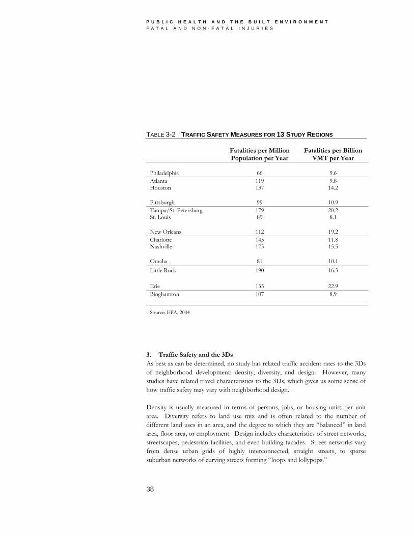
P U B L I C H E A L T H A N D T H E B U I L T E N V I R O N M E N T F A T A L A N D N O N - F A T A L I N J U R I E S
TABLE 3-2 TRAFFIC SAFETY MEASURES FOR 13 STUDY REGIONS
Fatalities per Million Population per Year
Fatalities per Billion VMT per Year
Philadelphia
66
9.6
Atlanta Houston
119 137
9.8 14.2
Pittsburgh
99
10.9
Tampa/St. Petersburg St. Louis
179 89
20.2 8.1
New Orleans
112
19.2
Charlotte Nashville
145 175
11.8 15.5
Omaha
81
10.1
Little Rock 190 16.3 Erie
135
22.9
Binghamton
107
8.9
Source: EPA, 2004
3. Traffic Safety and the 3Ds As best as can be determined, no study has related traffic accident rates to the 3Ds of neighborhood development: density, diversity, and design. However, many studies have related travel characteristics to the 3Ds, which gives us some sense of how traffic safety may vary with neighborhood design. Density is usually measured in terms of persons, jobs, or housing units per unit area. Diversity refers to land use mix and is often related to the number of different land uses in an area, and the degree to which they are “balanced” in land area, floor area, or employment. Design includes characteristics of street networks, streetscapes, pedestrian facilities, and even building facades. Street networks vary from dense urban grids of highly interconnected, straight streets, to sparse suburban networks of curving streets forming “loops and lollypops.”
38

P U B L I C H E A L T H A N D T H E B U I L T E N V I R O N M E N T F A T A L A N D N O N - F A T A L I N J U R I E S
FIGURE 3-1 AVERAGE RATE OF TRAFFIC FATALITIES VS. STRANGER HOMICIDES – PITTSBURGH METROPOLITAN AREA
Source: (Lucy and Rabalais, 2002) Starting in about 1990, researchers began to rigorously study the relationships of the 3Ds to travel behavior. Some 50 studies conducted during the decade were methodologically sophisticated, in that they used disaggregate travel data for individuals or households, made some effort to control for other influences on travel behavior, particularly socioeconomic status of travelers, and tested a wider variety of local land use, transportation, and site design variables than had earlier studies. A meta-analysis of these studies found that all 3Ds bear small but significant relationships to VMT (Ewing and Cervero, 2001). Elasticities are presented in Table 3-3. An elasticity is the percentage change in one variable with respect to a one percent change in another variable. Hence, from Table 3-3, we would expect a doubling of neighborhood density to result in a five percent reduction in VMT, and all else being equal, a five percent reduction in traffic accidents per capita. The effects of the 3Ds are independent and cumulative. Note that the elasticity of VMT with respect to regional accessibility is as large as the others combined. Regardless of the 3Ds, those living at highly accessible central locations are likely to generate substantially fewer VMT and many fewer accidents than their counterparts at the edge of the metropolitan area.
39

P U B L I C H E A L T H A N D T H E B U I L T E N V I R O N M E N T F A T A L A N D N O N - F A T A L I N J U R I E S
TABLE 3-3 TRAVEL ELASTICITIES OF THE 3DS/REGIONAL ACCESSIBILITY
Vehicle Trips (VT) Vehicle Miles Traveled
(VMT)
Local Density -.05 -.05
Local Diversity (Mix) -.03 -.05
Local Design -.05 -.03
Regional Accessibility -- -.20
Source: Ewing and Cervero, 2001
C. Traffic Safety and Road Network Design The traditional urban grid has short blocks, straight streets, and a crosshatched pattern. The typical contemporary suburban street network has large blocks, curving streets, and a branching pattern. The two prototypical networks differ in three respects: block size, degree of curvature, and degree of interconnectivity. Both network designs have advantages and disadvantages. Traditional grids disperse traffic rather than concentrating it at a handful of intersections. They offer more direct routes and hence generate fewer VMT than do contemporary networks. They encourage walking and biking with their direct routing and their alternatives to travel along high-volume streets. The most pedestrian-oriented cities in the world are those with the densest, web-like street networks. Grids are also more transit-friendly in that they allow transit vehicles to avoid backtracking and frequent turns, and offer transit users relatively direct access to transit stops. On the other hand, contemporary networks have some obvious advantages over grids. By keeping through-traffic out of neighborhoods, contemporary networks keep accident rates down and property values up. They may also discourage crime by making entry and escape relatively difficult for would-be offenders. Cul-de-sacs, the ultimate in disconnected streets, are quieter and safer for children to play in the
40

P U B L I C H E A L T H A N D T H E B U I L T E N V I R O N M E N T F A T A L A N D N O N - F A T A L I N J U R I E S
street, encourage more casual interaction among neighbors, and often command a premium in real estate markets. Which is better from the standpoint of traffic safety? It is hard to say since there has never been a credible network-wide comparison of the two. With the contemporary network, the concentration of traffic on a few roads and at a few intersections would tend to inflate accidents on these specific facilities. At the same time, the absence of through-traffic on local streets, and the lower density of intersections at which conflicts occur, would favor the contemporary network. One study compared accident rates in subdivisions with the two types of networks, referred to as “gridiron” and “limited-access” (Marks, 1957). These roughly correspond to the traditional and contemporary networks described above. The distribution of accidents was fairly uniform across the gridirons; accidents were concentrated wherever two continuous streets met at a four-way intersection. Where there were interruptions in the grid, creating three-way intersections, accidents were infrequent. The limited-access networks also had accidents concentrated at four-way intersections, but there were relatively few of these intersections in the network. The large number of T-intersections in the limited-access network had practically no accident history. Overall, the accident frequency for the five-year period studied was 77.7 accidents per year for the gridiron subdivisions and 10.2 accidents per year for the limited access subdivisions. Accident frequencies were dramatically higher for four-way than three-way intersections, regardless of the network type. Other research supports these findings (Staffeld, 1953; Bennett and Marland, 1978). The Marks study has been criticized for failing to consider the severity of accidents in the two networks, and the rate of accidents for the networks as a whole (not just the portion within subdivisions). Still, the main conclusion seems sound: the shorter the uninterrupted length of roadway, the slower the traffic will be. Short stretches ending in T-intersections are particularly effective in reducing speeds and accidents. D. Traffic Safety and Street Cross Sections Over the past 30 to 40 years, changes in engineering standards have resulted in roads that generally have fewer curves, fewer roadside objects, wider travel lanes, and more travel lanes. Fatalities per mile traveled have declined substantially over the same period. This has led to the belief that wide, straight, and open roads
41

P U B L I C H E A L T H A N D T H E B U I L T E N V I R O N M E N T F A T A L A N D N O N - F A T A L I N J U R I E S
improve traffic safety. This belief ignores confounding factors such as increased seatbelt use, and also ignores behavioral changes on the part of drivers in response to road improvements (possibly driving farther, faster, and less carefully). A study presented at the 2001 Annual Meeting of the Transportation Research Board found that, controlling for demographic changes, increased seatbelt use, and improved medical technology, highway improvements over the past 14 years had actually had a negative effect on highway safety (Noland, 2001; Noland, 2003). There were an estimated 2,000 additional fatalities and 300,000 or more additional injuries due to such “improvements.” Among infrastructure variables, increases in lane widths accounted for over half of the total increase in fatalities and about one-quarter of the increase in injuries. This finding is supported by an analysis of 20,000 crashes in the City of Longmont, Colorado, which found that crash rates increased exponentially with street width (Swift et al., pending). Of ten street variables tested, street width proved by far the most significant determinant of accident rates. The only other significant street characteristic was average daily traffic volume. 1. Mitigating the Effects of Speed Wider is not necessarily safer due to the mediating effect of roadway width on vehicle operating speed. The weight of evidence suggests that vehicle operating speeds decline somewhat as individual lanes and street sections are narrowed (Farouki and Nixon, 1976; Heimbach et al., 1983; Clark, 1985; Harwood, 1990; Gattis and Watts, 1999; Fitzpatrick et al., 2001; and Gattis, 2001). Beyond lower speeds, drivers seem to behave less aggressively on narrow streets, running fewer traffic signals, for example (Untermann, 1990). Also, drivers may feel less safe and drive more cautiously on narrow streets (Mahalel and Szternfeld, 1986 as referenced in: Noland, R. B., 2003). 2. Number of Lanes On two-lane roads, prudent drivers set the pace and others must follow. On multilane roads, aggressive drivers can pass slower drivers, and they tend to set the prevailing speed (Burden and Lagerwey, 1999). The conversion of an urban two-lane undivided road to four lanes typically produces a substantial increase in accident rates (Harwood, 1986). Studies finding that more lanes lead to more crashes include Milton and Mannering (1998), Sawalha and Sayed (2001), Vitaliano and Held (1991), and Noland and Oh (2004). The exception to this rule occurs when turn lanes are added to streets previously without them. The addition of turn lanes removes turning vehicles from through lanes, thereby reducing common rear-end collisions.
42

P U B L I C H E A L T H A N D T H E B U I L T E N V I R O N M E N T F A T A L A N D N O N - F A T A L I N J U R I E S
FIGURE 3- 2 AVERAGE LANE WIDTH VS. 85TH PERCENTILE SPEED
Source: Fitzpatrick et al., 2001 Conversely, when lanes are dropped, safety typically improves. A study presented at the 2001 Transportation Research Board Annual Meeting determined that 23 “road diet” projects, involving the reduction in cross section from four lanes to three lanes (two through lanes plus a center turn lane), produced crash reductions of two to 42 percent (Huang et al., 2001). In another study, conversions from undivided four-lane roads to three-lane roads with center turn lanes resulted in reductions in excessive speeds; total crashes by 17 to 62 percent (Knaap and Giese, 2001). 3. On-Street Parking The presence of on-street parking, such as on traditional shopping streets or residential streets, may also have an impact on safety. Parked cars act as a buffer between traffic and pedestrians. They are a convenience to shoppers and residents. However, these benefits may be realized at the expense of traffic safety. The available literature suggests that on-street parking accounts for a significant proportion of urban crashes (Seburn, 1967; Humphreys et al., 1978; Texas Transportation Institute, 1982; Box, 2000). If parking is permitted, conflicts with parked cars produce about 40 percent of total accidents on two-way major streets, 70 percent on local streets, and a higher percentage on one-way streets (Box, 2000).
43

P U B L I C H E A L T H A N D T H E B U I L T E N V I R O N M E N T F A T A L A N D N O N - F A T A L I N J U R I E S
The number of accidents increases with the parking turnover rate, meaning that land uses which generate high turnover will also generate more traffic accidents (Humphreys et al., 1978). Interestingly, no study of accident rates on comparable roadway sections with and without curbside parking, the ultimate test of on-street parking's safety impact, appears to have been completed to date. It is possible that where parking is provided, parked cars account for a large proportion of accidents, and yet overall accident rates are about the same as on sections without parking. E. Traffic Safety and Traffic Calming By reducing traffic speeds and/or traffic volumes, traffic calming should also reduce traffic accidents. The Insurance Corporation of British Columbia published a report titled Safety Benefits of Traffic Calming. In it, 43 international case studies were summarized. Among the 43, collision frequencies declined by anywhere from eight to 100 percent. Apparently in no case did collisions increase with traffic calming. Traffic circles and chicanes (s-shaped curves) had the most favorable impacts on safety, reducing collision frequency by an average of 82 percent, as shown in Figure 3- 3. It is easy to see why circles might have this effect; they are located at intersections, where a disproportionate number of traffic collisions occur. Circles not only slow traffic on the approaches but reduce the number of potential conflict points within the intersection from 21 to just eight. It is more difficult to understand why chicanes would have such a favorable impact on safety. Perhaps it is due to the heightened attention to driving that accompanies the relatively complex maneuver of negotiating an s-curve. It was not clear from the Insurance Corporation’s report whether the chicanes studied were one- or two-lane slow points. If one-lane slow points, driver attention would be further heightened by the narrow paved width and the potential for conflict with opposing traffic.
44

P U B L I C H E A L T H A N D T H E B U I L T E N V I R O N M E N T F A T A L A N D N O N - F A T A L I N J U R I E S
FIGURE 3- 3 AVERAGE REDUCTION IN COLLISIONS BY TRAFFIC CALMING MEASURE
Source: Geddes et al., 1996 In the international survey, humps were almost as effective as circles and chicanes, achieving an average collision reduction of 75 percent. This is counterintuitive. While humps slow traffic, they also create wide variations in speed within the traffic stream. Some vehicles slow down more than others, or slow down sooner than others. Variation in speed, as much as speed itself, is a cause of collisions. As for the U.S. experience, before-and-after studies of collisions are summarized in Traffic Calming State-of-the-Practice, a report co-published by the Institute of Transportation Engineers and Federal Highway Administrative (Ewing, 1999; also see Ewing, 2001). A difference-of-means test for paired samples was used to check for significant changes in collision frequencies after traffic calming measures were installed. Test results are provided in Table 3-4. The test was applied to the entire sample and to subsamples of different traffic calming measures. The test was also applied to the subsample of measures for which before-and-after traffic volumes were available, adjusting collision frequencies after traffic calming for changes in traffic volumes and hence changes in exposure. For the sample as a whole,
45

P U B L I C H E A L T H A N D T H E B U I L T E N V I R O N M E N T F A T A L A N D N O N - F A T A L I N J U R I E S
collisions decline to a very significant degree after traffic calming (the difference being statistically significant at the .001 probability level). Adjusting for changes in traffic volumes, and dropping cases for which volume data are not available, collisions decline to a less significant degree (but still statistically significant at the conventional .05 level). As for individual traffic calming measures, all reduce the average number of collisions on treated streets, and 22-foot tables and traffic circles produce differences that are statistically significant. Including Seattle data when traffic circles have produced dramatic improvements in safety, circles are by far the best performers. It is curious that safety impacts of traffic calming in the U.S., while favorable, would be less favorable then outside the U.S. One possible explanation is that European and British traffic calming treatments are more intensive and more integrated with their surroundings than U.S. treatments. Three illustrated volumes—one continental European, one British, and one a mix—clearly demonstrate this point (Herrstedt et al., 1993; County Surveyors Society, 1994; and Hass-Klau, C., et al., 1992). Hardly a treatment pictured or described has only one type of measure in place; most make use of two or three at a single slow point to calm traffic intensively. Reported speeds drop on average by almost 11 mph or 30 percent in the British sample, compared to under 7 mph or 20 percent for U.S. studies collected for Traffic Calming State-of-the-Practice (Ewing, 1999). All the traffic calming literature referenced so far relates to traffic accidents generally. One recent study showed that the presence of speed humps on a street was associated with lower odds of child pedestrians being injured within their neighborhoods and being struck in front of their homes (Tester et al., 2004). F. Traffic Safety and Access Management Access management is the control of the location, spacing, and operation of driveways, median openings, and street connections to a roadway. Generally, the more that access to abutting property is limited on main roads, the safer their operation. In particular, major roadways cluttered with driveways have more conflict points and afford drivers reduced response time when conflicts arise.
46

P U B L I C H E A L T H A N D T H E B U I L T E N V I R O N M E N T F A T A L A N D N O N - F A T A L I N J U R I E S
TABLE 3-4 SAFETY IMPACTS OF TRAFFIC CALMING MEASURES
No. of Observati
ons
Average No. of Collisions Before/After Treatment
% Change in Collisions
Before->After
Treatment
t-statistic (significance level—two-tailed test)
Humps 54 2.8/2.4 -14% -1.2 (.22)
22' Tables 51 1.5/.8 -47% -3.0 (.005)
Circles without Seattle Circles with Seattle
17 130
5.9/4.2 2.2/.6
-29% -73%
-2.2 (.05) -10.8 (.001)
All Measures w/out adjustments w/ adjustments
235 47
2.2/1.1
1.8/1.2
-50% -33%
-8.6 (.001) -2.5 (.05)
Source: Ewing, 2001
The main study of access management’s safety benefits is the Transportation Research Board’s Impacts of Access Management Techniques (Gluck et al., 1999). This study found that as the density of access points decreases, so do crash rates. This study also found that as conflicts between opposing traffic are eliminated by raised medians (non-traversable medians, which limit access), crash rates decline. The dual effects of these two variables—access point density and non-traversable medians—are reflected in Table 3-5. Other studies reaching similar conclusions are summarized in the Transportation Research Board’s Access Management Manual (Committee on Access Management, 2003). In general, it appears that crash rates increase with the square root of the increase in access density, up to about 40 access points per mile. Various studies are summarized in Figure 3- 4.
47

P U B L I C H E A L T H A N D T H E B U I L T E N V I R O N M E N T F A T A L A N D N O N - F A T A L I N J U R I E S
TABLE 3-5 URBAN AND SUBURBAN CRASH RATES BY LEVEL OF ACCESS CONTROL (PER MILLION VEHICLE MILES)
Median Type
Total Access Points per Mile Undivided
Two-Way Left-Turn Lane
Non-Traversable Median
≤20 3.8 3.4 2.9
20-40 7.3 5.9 5.1
40-60 9.4 7.9 6.8
>60 10.6 9.2 8.2
Source: Gluck et al., 1999, p. 4
In most but not all studies, roads with raised medians (non-traversable medians, which limit access) appear safer than roads with center two-way left-turn lanes. Both of these design options appear safer than undivided roads. An additional important effect of raised medians is to improve pedestrian safety by providing a refuge area for pedestrians crossing a roadway, a refuge absent from other cross sections. Pedestrians can cross in two stages, simplifying the crossing task. This is especially helpful for older pedestrians who walk at slower speeds. A study of pedestrian-vehicle crash experience on arterial roadways in Atlanta, Phoenix, and Los Angeles found that crash rates were about the same for undivided roadways and roadways with center two-way left-turn lanes, but considering both intersection and mid-block accidents, crash rates were about half as high on arterials with raised medians. Figure 3-5 shows the pedestrian crash rates for suburban arterials with different cross sections.
48
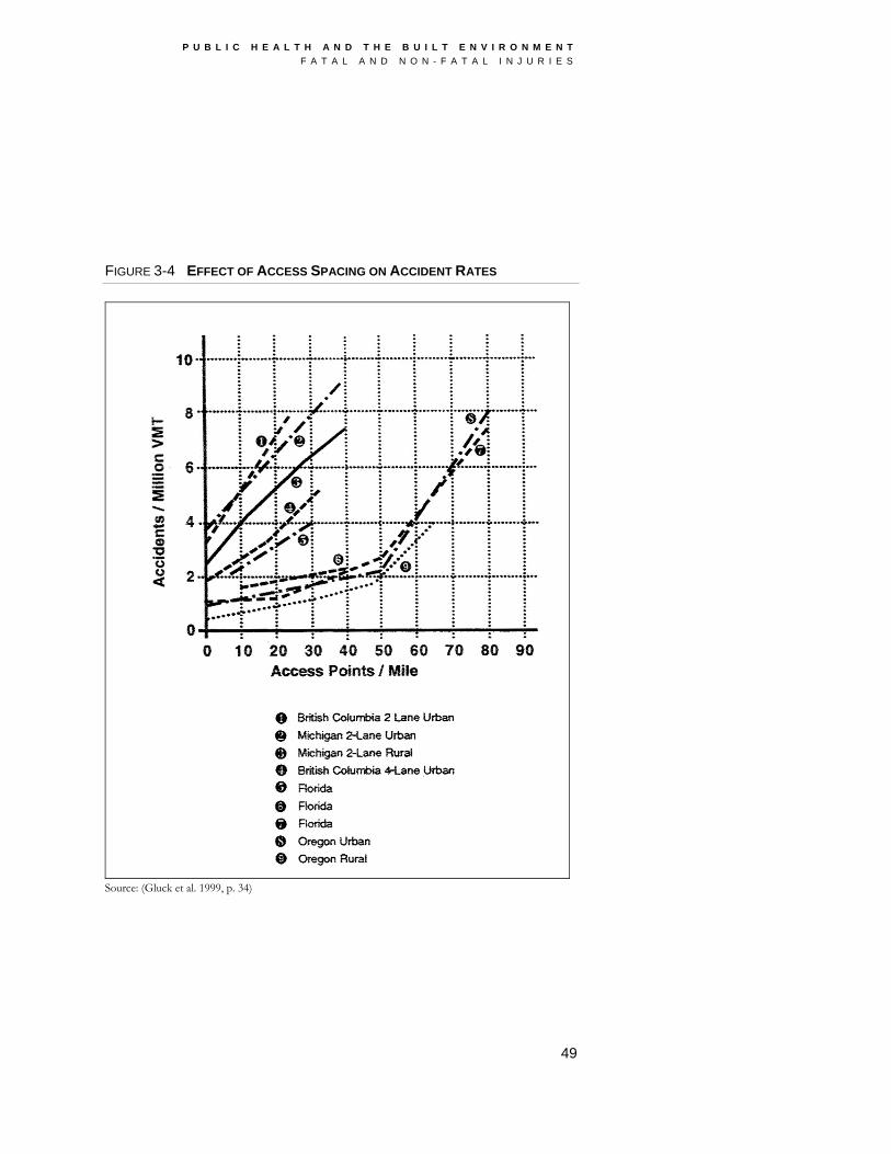
P U B L I C H E A L T H A N D T H E B U I L T E N V I R O N M E N T F A T A L A N D N O N - F A T A L I N J U R I E S
FIGURE 3-4 EFFECT OF ACCESS SPACING ON ACCIDENT RATES
Source: (Gluck et al. 1999, p. 34)
49

P U B L I C H E A L T H A N D T H E B U I L T E N V I R O N M E N T F A T A L A N D N O N - F A T A L I N J U R I E S
Safety benefits of medians appear to vary with median width. Research in Adelaide, South Australia, found that pedestrian accident rates on arterial roads have an orderly relationship to median width, with the narrowest medians (four feet) having four times the pedestrian crash rate of those with the widest median (ten feet) (Scriven 1986). Replacing a 6-foot painted median with a wide raised median reduced pedestrian accidents by 23 percent (Claessen and Jones 1994). Traffic safety benefits associated with a variety of access management techniques are summarized by S&K Transportation Consultants (2000). They range from a 20 percent reduction in accidents associated with the addition of right turn bays, to a 67 percent reduction associated with the addition of left-turn dividers. G. Traffic Safety and Intersection Traffic Control Crash frequencies depend on the form of traffic control applied to intersections. Where traffic volumes are high enough to warrant traffic signals butnot high enough to absolutely require them, all-way stop signs and roundabouts may be considered instead. All-way stop signs are not favored by traffic engineers but are well-liked by citizens who value their traffic calming effect and the minimal delays they cause under light traffic conditions. From a safety standpoint, all-way stops appear to outperform signals at moderate traffic volumes, say, up to 10,000 vehicles per day on the major street (Syrek, 1955; Ebbecke and Schuster, 1977; Bissell and Neudorff, 1980). One study found that pedestrian collisions declined by 25 percent when traffic signals were converted to all-way stops at low-volume urban intersections (Persaud et al., 1997.)
50

P U B L I C H E A L T H A N D T H E B U I L T E N V I R O N M E N T F A T A L A N D N O N - F A T A L I N J U R I E S
FIGURE 3- 5 PEDESTRIAN CRASH RATES ON SUBURBAN ARTERIALS
Source: (Bowman and Vecellio, 1994) from Access Management Manual Note: Suburban arterials measured had different cross sections: undivided two-way traffic (undivided); two-way, left turn lane configuration (TWLTL); or a configuration with non-traversable median. U.S. traffic engineers have not favored roundabouts either, but this is largely a case of mistaken identity; modern roundabouts are mistaken for old-fashioned traffic circles. The virtues of roundabouts are beginning to be acknowledged at transportation conferences and in transportation journals. Specifically, they allow traffic from different directions to share space in the intersection, while signals require traffic to take turns. Thus, roundabouts have more capacity and produce shorter delays when traffic flows are moderate and somewhat balanced. If properly designed, roundabouts also have a significant safety advantage. Yield and deflection at entry, and the curvature of the travel path through the intersection, reduce travel speeds. Counter-clockwise circulation around the center island reduces the number of conflict points, eliminating certain types of collisions such as right angle and left turn head-on crashes. Several studies have concluded that roundabouts outperform other intersection control devices with respect to safety (Maycock and Hall, 1984; Ourston, 1993; Schoon and van Minnen, 1993; Flannery and Datta, 1996; Jacquemart, 1998; Robinson et al., 2000; Persuad et al., 2002). Even where crash frequencies are comparable to other intersections, crash severity is lessened (Brown, 1995).
51

P U B L I C H E A L T H A N D T H E B U I L T E N V I R O N M E N T F A T A L A N D N O N - F A T A L I N J U R I E S
Persuad et al. (2002) evaluated the change in crash rates following the conversion of 24 intersections to modern roundabouts in the United States. The study used a before-and-after study design. The intersections evaluated were from eight states. There was a significant overall reduction of 39 percent in crash rates. For crashes involving injuries, reductions amounted to 76 percent. Crashes involving deaths or incapacitating injuries fell by about 90 percent. This same study addressed a common concern that older drivers may have difficulty adjusting to roundabouts. It found no increase in the average age of crash-involved drivers following the installation of roundabouts, suggesting that roundabouts do not pose a problem for older drivers. Small and medium capacity roundabouts are safer than large or multilane roundabouts (Maycock and Hall, 1984; Alphand et al., 1991). Crash reductions are most pronounced for motor vehicles, less pronounced for pedestrians, and equivocal for bicyclists, depending on the study and bicycle design treatments (Alphand et al., 1991; Schoon and van Minnen, 1993; Schoon and van Minnen, 1994; Brown, 1995). Single-lane roundabouts, in particular, have been reported to produce substantially lower pedestrian crash rates than comparable intersections with traffic signals (Brude and Larsson, 2000.) Comparative crash statistics from one study are presented in Table 3-6. While the European experience with roundabouts suggests that they are relatively safe for pedestrians and bicyclists, there remains in the United States a preference for traffic signals at locations with heavy pedestrian and bicycle traffic. Signals provide a periodic gap in traffic for crossing pedestrians, while the continuous flow of roundabouts does not. Signals require no deflection of motor vehicles crossing an intersection, while roundabouts may cause motorists to cross paths with bicyclists. H. Traffic Safety and the Roadside Environment It is conventional engineering practice to keep large trees, utility poles, and other fixed objects away from the roadway edge. The rationale for doing so is safety-related: given a wide clear zone, motorists leaving the roadway can safely recover before encountering a hazardous fixed object. Whether this practice actually enhances safety, however, is subject to debate. It ignores the possibility that having a wide open roadside may affect behavior, causing drivers to go faster and exercise
52

P U B L I C H E A L T H A N D T H E B U I L T E N V I R O N M E N T F A T A L A N D N O N - F A T A L I N J U R I E S
TABLE 3-6 PEDESTRIANS CRASH RATES VS. TYPE OF CROSSING
Intersection Type Pedestrian Crashes per Million Trips
Mini-roundabout 0.31
Conventional roundabout 0.45
Flared roundabout 0.33
Signals 0.67
Source: Robinson et al., 2000, p. 117
Note: British Crash Rates.
less care than they would in more defined and enclosed street space (Dumbaugh, 2005). The empirical evidence on this subject is mixed. Zegeer et. al. (1988: 39) report: “[d]rastic reductions in single-vehicle accident rates … for increases in average recovery distance, particularly beyond ten feet”. The safety benefits of a clear zone, at least beyond 10 feet, are more limited in urban areas, as shown in Table 3-7. This finding seems particularly applicable to rural sections. The safety benefits of a clear zone, at least beyond ten feet, are more limited in urban areas. Naderi (2003) examined the safety impacts of aesthetic streetscape enhancements placed along the roadside and medians of five arterial roadways in downtown Toronto. This study found that the inclusion of features such as trees and concrete planters resulted in statistically-significant reductions in the number of mid-block crashes along all five of the roadways, with the number of crashes decreasing from between five and 20 percent as a result of the streetscape improvements. The author attributed this reduction to the presence of a well-defined roadside edge, leading drivers to exercise greater caution while driving. Another study which suggests a positive effect of roadside trees is by Lee and Mannering (1999). While their model for rural areas performed as expected, with trees and other features being associated with statistically-significant increases in
53

P U B L I C H E A L T H A N D T H E B U I L T E N V I R O N M E N T F A T A L A N D N O N - F A T A L I N J U R I E S
the number of roadside crashes that occur, their model for urban areas produced radically different results. The presence of trees in urban areas was associated with a decrease in the probability of a roadside crash. The number of sign supports was also associated with crash reductions, as were the presence of miscellaneous fixed-objects, including mailboxes and telephone booths. Further, wider lanes and shoulders were associated with statistically-significant increases in crash frequencies. Dumbaugh (2005) provides other examples of tree-lined street sections producing fewer accidents than control sections with wide clear zones. On balance, it would appear that having trees and other vertical elements close to a roadway in a low-speed urban setting may actually enhance safety, contrary to engineering theory and practice. I. Traffic Safety and Pedestrian Countermeasures Pedestrian countermeasures are engineering actions taken to improve the safety of roadways for pedestrians. One study classified countermeasures into three broad categories: separation of pedestrians from vehicles by time and space; measures that increase the visibility and conspicuity of pedestrians; and reductions in vehicle speed (the last of these already covered under the heading of traffic calming) (Retting et al., 2003). The Pedestrian Facilities Users Guide lists 47 such measures (Zegeer et al., 2001). Most of the studies of pedestrian countermeasures have used proxies for traffic safety to document impacts. Travel speeds have been measured in some cases, conflict counts and yielding behavior in others. Actual accident rates are seldom measured in such studies. This may not constitute as big a shortcoming as would at first appear, however, since conflict counts have been shown to provide an accurate estimate of multi-year crash rates (Hauer and Garder, 1986). Sidewalks are an absolute necessity along all through-streets serving developed areas. Pedestrian accidents are more likely on street sections without sidewalks than those with them, two and one-half times more likely according to one study (Tobey et al., 1983; Knoblauch et al., 1988). Sidewalk clearances, vertical curbs, street trees between street and sidewalk, and parked cars all add to the sense of security.
54

P U B L I C H E A L T H A N D T H E B U I L T E N V I R O N M E N T F A T A L A N D N O N - F A T A L I N J U R I E S
TABLE 3-7 ACCIDENT RATES BY LANE WIDTH AND ROADSIDE RECOVERY
Average Roadside Recovery Distance (ft)
Lane Width (ft) 0 to 5 6 to 10 11 to 15 16 to 30
< 10 105 (14) 76 (11) 24 (10) 23 (5)
11 130 (4) 100 (15) 54 (17) 27 (7)
> 12 135 (15) 97 (15) 74 (19) 56 (11)
( ) = Numbers of sample sections are given in parentheses
Source: Zegeer et. al., 1988
Note: Rates reflect single-vehicle accident rates (ACC/100 MVM) by lane width and average roadside recovery distance for urban sections in seven states.
The most studied pedestrian countermeasure is the installation of marked crosswalks. Crosswalks are nearly always marked at signal- and stopped-controlled intersections, and the fact that traffic is forced to stop at these intersections means that pedestrian crossings are relatively safe, with or without marked crosswalks. The issue is whether it enhances safety to mark crosswalks at uncontrolled intersections and midblock locations. In one study of uncontrolled locations, drivers were found to approach pedestrians in a crosswalk somewhat slower, and crosswalk usage was found to increase after markings were installed (Knoblauch et al., 2001). However, this study found no changes in driver yielding behavior or pedestrian assertiveness. Overall, the study concluded that marking pedestrian crosswalks at relatively low-speed, low volume, unsignalized intersections is a desirable practice. Another study evaluated driver speeds before and after installation of crosswalk markings at uncontrolled intersections (Knoblauch and Raymond, 2000). Speed data were collected under three conditions: no pedestrian present, pedestrian looking, and pedestrian not looking. Overall, there was a significant reduction in speed under both the no pedestrian and the pedestrian not looking conditions. It appeared that crosswalk markings made drivers on relatively low-speed arterials more cautious and more aware of pedestrians.
55

P U B L I C H E A L T H A N D T H E B U I L T E N V I R O N M E N T F A T A L A N D N O N - F A T A L I N J U R I E S
FIGURE 3- 6 PEDESTRIAN CRASH RATE VS. TYPE OF CROSSING
Source: Zegeer et al., 2002, p. 8 The most ambitious study of crosswalks at uncontrolled locations involved a comparison of five years of pedestrian crashes at 1,000 marked crosswalks and 1,000 matched unmarked comparison sites. All sites in this study lacked traffic signals or stop signs on the approaches (Zegeer et al., 2002). As shown in Figure 3- 6, the study results revealed that on two-lane roads, the presence of a marked crosswalk alone at an uncontrolled location was associated with no difference in pedestrian crash rate, compared to an unmarked crossing. Further, on multi-lane roads with traffic volumes above about 12,000 vehicles per day, having a marked crosswalk alone (without other substantial improvements) was associated with higher pedestrian crash rates (after controlling for other site factors) compared to an unmarked crossing. Raised medians provided significantly lower pedestrian crash rates on multi-lane roads, compared to roads with no raised median. Studies from other countries speak to the safety benefits of pedestrian activated signals at uncontrolled crossing points. Installing so-called Pelican signals was highly effective in reducing crashes in Australia (Geoplan, 1994). The Pelican
56

P U B L I C H E A L T H A N D T H E B U I L T E N V I R O N M E N T F A T A L A N D N O N - F A T A L I N J U R I E S
signal is similar to a standard mid-block pedestrian signal, except that during the pedestrian clearance phase, the display facing motorists changes to a flashing yellow, indicating that vehicles may proceed cautiously through the crossing but are required to yield to pedestrians. In this way these signals produce less delay for motorists than standard pedestrian activated signals. Compared to untreated sites, the estimated reduction in pedestrian collisions was 87 percent, which was statistically significant. Installing standard pedestrian-activated signals at mid-block locations also gave rise to statistically significant reductions in crashes. In this case the adjusted reduction was 49 percent. Support for the safety benefits of refuge islands is less certain (Cairney, 1999). The Geoplan study included four types of pedestrian refuge — those with curb extensions and those without curb extensions, either on existing pedestrian crossings, or on their own. None of them were particularly effective. Refuges with curb extensions actually resulted in an increase in pedestrian crashes; when this was corrected for the reduction in crashes at comparison sites, it resulted in an adjusted crash rate which showed a 53 percent increase. Refuges without curb extensions on existing crossings resulted in no changes in crashes which produced an adjusted rate of a 38 percent increase. Refuges on their own without curb extensions resulted in a 15 percent reduction in crashes, producing an adjusted rate of a 14 percent increase. Only refuges with curb extensions achieved an adjusted rate that was actually a reduction, and that was only two percent. However, in view of the other findings discussed above, it seems inherently likely that pedestrian refuges did reduce crashes. The method used in the Geoplan study compared crashes occurring at the site of the facility, before and after. Where pedestrian refuges are provided, it would be expected that pedestrians would be attracted to cross at this point — pedestrians who would otherwise have crossed some distance along the road, so that pedestrian flow is greatly increased at the refuge. A study of the crash history of the whole street where pedestrian refuges have been installed would therefore be necessary to determine whether there had been a reduction in pedestrian crashes. J. Conclusion The incidence of fatal and non-fatal injuries as a result of traffic accidents is closely related to vehicle miles traveled, automobile speed and traffic volumes. These characteristics of travel have been linked in the research to the design of the roadway and street network and the distribution of land uses. In particular,
57
P U B L I C H E A L T H A N D T H E B U I L T E N V I R O N M E N T F A T A L A N D N O N - F A T A L I N J U R I E S
development patterns that increase VMT. vehicle speed and traffic volume increase accident rates. K. References American Association of State Highway and Transportation Officials (AASHTO), A Policy on Geometric Design of State Highways and Streets, Washington, D.C., 2001. Abdel-Aty, M.A. and Radwan, A.E. (2000) “Modeling Traffic Accident Occurrence and Involvement,” Accident Analysis and Prevention, 32, 633-642. Bennett, G.T. and Marland, J, 1978, Road Accidents in Traditionally Designed Residential Estates, Supplementary Report 394, Transportation Road Research Laboratory, Crowthorne, England. Bissell, H.H. and Neudorff, L.G., "Criteria for Removing Traffic Signals," ITE 1980 Compendium of Technical Papers, Institute of Transportation Engineers, Washington, D.C., 1980, pages 56-66. Bowman, B.L. and R.L. Vecellio (1994). “Effect of Urban and Suburban Median Types on Both Vehicular and Pedestrian Safety,” Transportation Research Record 1445, pages 169-179. Box, P.C., “Curb Parking Findings Revisited,” Transportation Research E-Circular, Transportation Research Board, December 2000, pages B5/1-8. Brilon, W. and Blanke, H. (1993) “Extensive Traffic Calming: Results of Accident Analyses in Six Model Towns,” Proceedings of the 63rd Annual Meeting of the Institute of Transportation Engineers, Institute of Transportation Engineers, Washington, D.C., 119-123. Brude, U. and Larsson, J. (2000) “What Roundabout Design Provides the Highest Possible Safety?” Nordic Road Transport Research, 12: 17-21. Bunn, F., Collier, T., Frost, C., Ker, K., Roberts, I, and Wentz, R. (2003) Area-Wide Traffic Calming for Preventing Traffic Related Injuries, Update Software, Oxford, England. Burden, D. and Lagerwey, P, 1999, Road Diets: Fixing the Big Roads. Walkable Communities, High Springs, FL.
58

P U B L I C H E A L T H A N D T H E B U I L T E N V I R O N M E N T F A T A L A N D N O N - F A T A L I N J U R I E S
Cairney, P., Pedestrian Safety in Australia, FHWA-RD-99-093, Federal Highway Administration, Washington, D.C., 1999. Claessen, J.G. and Jones, D.R., (1994). “The Road Safety Effectiveness of Raised Wide Medians.” Proceedings of the 17th Australian Road Research Board Conference 17, (5), pp 269-287. Clark, J.E., 1985, "High Speeds and Volumes on Residential Streets: An Analysis of Physical Street Characteristics as Causes in Sacramento, California," ITE 1985 Compendium of Technical Papers, Institute of Transportation Engineers, Washington, D.C., pages 93-96. Committee on Access Management (2003). Access Management Manual, Transportation Research Board, Washington, D.C., pages 15-20. County Surveyors Society, Traffic Calming in Practice, Landor Publishing, London, 1994. Dumbaugh, E. “Safe Streets, Livable Streets,” Journal of the American Planning Association, 2005, in press. Durning, A.T, 1996, The Car and the City: 24Steps to Safe Streets and Healthy Communities, Northwest Environmental Watch, Seattle, WA. Ebbecke, G.M. and Schuster, J.J., "Areawide Impact of Traffic Control Devices," Transportation Research Record 644, 1977, pages 54-57. Ewing, R., R. Pendall and D. Chen, "Measuring Sprawl and Its Transportation Impacts," Transportation Research Record 1832, 2003, pages 175-183. Ewing, R., R. Pendall and D. Chen, Measuring Sprawl and Its Impact, Smart Growth America/U.S. Environmental Protection Agency, Washington, D.C., 2002 . Ewing, R., R. Schieber and C. Zegeer, "Urban Sprawl as a Risk Factor in Motor Vehicle Occupant and Pedestrian Fatalities," American Journal of Public Health, Vol. 93, September 2003, pages 1541-1545. Ewing, R., Traffic Calming State-of-the-Practice, Institute of Transportation Engineers, Washington, D.C., 1999.
59

P U B L I C H E A L T H A N D T H E B U I L T E N V I R O N M E N T F A T A L A N D N O N - F A T A L I N J U R I E S
Farouki, O.T. and Nixon, W.J., 1976, "The Effect of Width of Suburban Roads on the Mean Free Speed of Cars," Traffic Engineering and Control, Vol. 17, pages 518-519. Fitzpatrick, K., Carlson, P., Brewer, M., and Wooldridge, M., 2001, “Design Factors that Affect Driver Speed on Suburban Streets,” Transportation Research Record 1751, pages 18-25. Flannery, A. and Datta, T.K., "Modern Roundabouts and Traffic Crash Experience in the United States," Paper presented at the 75th Annual Meeting, Transportation Research Board, Washington, D.C., 1996. Florida Department of Transportation (FDOT), Florida Roundabout Guide, Tallahassee, FL, 1998. Garder, P. (1989) “Pedestrian Safety at Traffic Signals: A Study Carried Out with the Help of a Traffic Conflicts Technique,” Accident Analysis and Prevention, Vol. 21, pages 435-444. Gattis, J.L., “Urban Street Cross Section and Speed Issues,” Transportation Research E-Circular, Transportation Research Board, December 2000. Gattis, J. L., and Watts, A., 1999, Urban Street Speed Related to Width and Functional Class, Journal of Transportation Engineering, Volume. 125, Issues. 3, pages 193–200. Geddes, E. et al., Safety Benefits of Traffic Calming, Insurance Corporation of British Columbia, Vancouver, British Columbia, 1996. Leaf, W.A. and Preusser, D.F, 1999, Literature Review on Vehicle Travel Speeds and Pedestrian Injuries, National Highway Traffic Safety Administration, Washington, D.C. Geoplan (1994). Evaluation of Pedestrian Road Safety Facilities. Report prepared for the Road Safety Bureau, Roads and Traffic Authority (New South Wales) by Geoplan Urban and Traffic Planning. Gluck, J., H.S. Levinson, and V. Stover (1999). Impacts of Access Management Techniques, NCHRP Report 420, Transportation Research Board, Washington, D.C., 1999.
60
P U B L I C H E A L T H A N D T H E B U I L T E N V I R O N M E N T F A T A L A N D N O N - F A T A L I N J U R I E S
Hakkert, AS, Gitelman, V, and Ben-Shabet, E. (2001) “An Evaluation of Crosswalk Warning Systems,” Proceedings of the 80th Annual Meeting of the Transportation Research Board (CD-ROM), Transportation Research Board, Washington, D.C. Harwood, D.W., 1990, Effective Utilization of Street Width on Urban Arterials. National Cooperative Highway Research Program Report 330. Transportation Research Board, National Research Council, Washington, D.C. Harwood, D.W. (1986) Multilane Design Alternatives for Improving Suburban Highways, NCHRP Report 282, Transportation Research Board, Washington, D.C. Hass-Klau, C., et al., Civilized Streets: A Guide to Traffic Calming, Environmental & Transport Planning, Brighton, England, 1992. Hauer, E., and Garder, P. (1986) “Research Into the Validity of the Traffic Conflicts Technique,” Accident Analysis and Prevention, 18: 471-481. Head, J.A. (1959) “Predicting Traffic Accidents from Roadway Elements on Urban Extensions of State Highways,” Bulletin No. 208, Highway Research Board. Heimbach, C.L., Cribbins, P.D., and Chang, M.S., 1983, "Some Partial Consequences of Reduced Traffic Lane Widths on Urban Arterials," Transportation Research Record 923, pages 69-72. Herrstedt, L., et al., An Improved Traffic Environment—A Catalogue of Ideas, Danish Road Directorate, Copenhagen, Denmark, 1993. Huang, H.F., Stewart, J.R., and Zegeer, C.V., “Evaluation of Lane Reduction ‘Road Diet’ Measures on Crashes and Injuries,” Transportation Research Record 1784, Washington, D.C., 2002, pages 80-90. Hummer, J.E. and Lewis, C.F., Operational Capacity of Three-Lane Cross-Sections, Report FHWA/NC/2000-003, Center for Transportation Engineering Studies, North Carolina State University, Raleigh, NC, 2000. Humphreys, J.B., et al., Safety Aspects of Curb Parking, Federal Highway Administration, Washington, D.C., 1978. "Impacts of Traffic Calming," Transportation Quarterly, Winter 2001, pages 33-45.
61

P U B L I C H E A L T H A N D T H E B U I L T E N V I R O N M E N T F A T A L A N D N O N - F A T A L I N J U R I E S
Jacobsen, P, et al, “Child Pedestrian Injuries on Residential Streets: Implications for Traffic Engineering,” ITE Journal on the Web, February 2000, pages 71-75. Jacquemart, G. Synthesis of Highway Practice 264: Modern Roundabout Practice in the United States. National Cooperative Highway Research Program. Washington, D.C: National Academy Press, 1998. Johnson, R.E. (1962). “Experience with Narrow Medians.” Proceedings of the 1st Australian Road Research Board Conference, 1 (1), pp 489-499. Knaap, K.K. and Giese, K., Guidelines for the Conversion of Urban Four-Lane Undivided Roadways to Three-Lane Two-Way Left-Turn Facilities, Center for Transportation Research and Education, Iowa State University, Ames, 2001. Knoblauch, R.L. et al., Investigation of Exposure Based Pedestrian Accident Areas: Crosswalks, Sidewalks, Local Streets and Major Arterials, Federal Highway Administration, Washington, D.C., 1988, pages 126-133. Knoblauch, R.L., M. Nitzburg, and R.F. Seifert, Pedestrian Crosswalk Case Studies: Sacramento, California; Richmond, Virginia; Buffalo, New York; Stillwater, Minnesota, Report No. FHWA-RD-00-103, Federal Highway Administration, McLean, VA, 2001. Knoblauch, R.L. and Raymond, P.D., The Effect of Crosswalk Markings on Vehicle Speeds in Maryland, Virginia, and Arizona, Report No. FHWA-RD-00-101, Federal Highway Administration, McLean, VA, 2000. Leden, L, Gårdner, P, Pulkkinen, U, 2000, “An Expert Judgment Mode Applied to Estimating the Safety Effect of a Bicycle Facility,” Accident Analysis and Prevention. Volume 32, pages 589–99. Leden, L, 2002, “Pedestrian Risk Decrease with Pedestrian Flow. A Case Study Based on Data from Signalised Intersections in Hamilton, Ontario.” Accident Analysis and Preventio. Volume 34, pages 457–64. Lee, J. and F. Mannering, Analysis of Roadside Accident Frequency and Severity and Roadside Safety Management. Washington State Department of Transportation. December, 1999.
62

P U B L I C H E A L T H A N D T H E B U I L T E N V I R O N M E N T F A T A L A N D N O N - F A T A L I N J U R I E S
Leong, H.J.W. (1970). “The Effect of Kerbed Median Strips on Accidents on Urban Roads.” Proceedings of the 5th Australian Road Research Board Conference, 5 (3), pp 338-364. Litman, T. (2004). “Safe Travels: Evaluating Mobility Management Traffic Safety Impacts.” Victoria Transport Policy Institute. Victoria, BC. Lucy, W. (2003) “Mortality Rish Associated with Leaving Home: Recognized the Relevance of the Built Environment,” American Journal of Public Health, 93(9), Lucy, W. and Rabalais, R. (2002) Traffic Fatalities and Homicides by Strangers: Danger of Leaving Home in Cities, Inner Suburbs, and Outer Suburbs, University of Virginia, Charlottesville Mahalel, D. and Szternfeld, Z. (1986) “Safety Improvements and Driver Perception,” Accident Analysis and Prevention, 18(1), 37-42 Marks, H, 1957, "Subdividing for Traffic Safety," Traffic Quarterly, 11(3), pages 308-325. Maycock, G., and R.D. Hall. “Crashes at four-arm roundabouts.” TRRL Laboratory Report LR 1120. Crowthorne, England: Transport and Road Research Laboratory, 1984. Milton, J. and Mannering, F. (1998) “The Relationship Among Highway Geometrics, Traffic-Related Elements and Motor-Vehicle Accident Frequencies,” Transportation, 25, 395-413. Naderi, J.R. Landscape Design in Clear Zone: Effect of Landscape Variables on Pedestrian Health and Driver Safety. Transportation Research 1851, 2003, pages 119-130. Noland, R. B., 2003. “Traffic Fatalities and Injuries: The Effects of Changes in Infrastructure and Other Trends.” Accident Analysis and Prevention 35, pages 599-611. Noland, R, 2001, “Traffic Fatalities and Injuries: Are Reductions the Result of ‘Improvements’ in Highway Design Standards,” paper presented at the 80th Annual Meeting, Transportation Research Board, Washington, D.C.
63

P U B L I C H E A L T H A N D T H E B U I L T E N V I R O N M E N T F A T A L A N D N O N - F A T A L I N J U R I E S
Noland, R. B., and Oh, L, 2004, “The Effect of Infrastructure and Demographic Change on Traffic-Related Fatalities and Crashes: A Case Study of Illinois County-Level Data.” Accident Analysis and Prevention 36, pages 525-532. Ourston, L., "A Synthesis of Roundabout Safety Research, with Recent Increases in Numbers of Roundabouts in a Few Countries," Unpublished manuscript available from the author, Leif Ourston & Associates, Santa Barbara, CA, 1993. Peltzman, S. (1975) “The Effects of Automobile Safety Regulation,” Journal of Political Economy, 83, 677-725. Persuad, B. N., R. A. Retting, P. E. Garder, and D. Lord. (2002). “Crash Reductions Following Installation of Roundabouts in the United States.” Insurance Institute for Highway Safety, Arlington, VA Persaud, B., E. Hauer, R.A. Retting, Vallurupalli, R., and K. Mucsi (1997) “Crash Reductions Related to Traffic Signal Removal in Philadelphia,” Accident Analysis and Prevention, 29: 803-810. Peterson, P, et al, “Child Pedestrian Injuries on Residential Streets: Implications for Traffic Engineering,” ITE Journal on the Web, Feb. 2000, pages 71-75. Prevedouros, P.D. (2001) “Evaluation of In-Pavement Flashing Lights on a Six-Lane Arterial Pedestrian Crossing,” Proceedings of the 71st Annual Meeting of the Institute of Transportation Engineers (CD-ROM), Institute of Transportation Engineers, Washington, D.C. R. Van Houten and J.E.L. Malenfant, Canadian Research on Pedestrian Safety, Federal Highway Administration, McLean, VA., 1999. Roberts, I., Norton, R., Jackson, R., Dunn, R., Hassal, I, 1995, “Effect of Environmental Factors on Risk of Injury of Child Pedestrians by Motor Vehicles: A Case-Control Study,” British Medical Journal (310) 91-94. S&K Transportation Consultants (2000) Access Management, Location and Design. Participant notebook for NHI Course 133078, National Highway Institute, Federal Highway Administration, Washington, D.C. Sawalha, Z. and Sayed, T. (2001) “Evaluating Safety on Urban Arterial Roadways,” Journal of Transportation Engineering, 127(2), 151-158.
64
P U B L I C H E A L T H A N D T H E B U I L T E N V I R O N M E N T F A T A L A N D N O N - F A T A L I N J U R I E S
Schoon, C.C., and J. van Minnen. (1993) Accidents on Roundabouts: II. Second study into the road hazard presented by roundabouts, particularly with regard to cyclists and moped riders. R-93-16. The Netherlands: SWOV Institute for Road Safety Research. Schoon, C.C. and J. van Minnen (1994) “The Safety of Roundabouts in the Netherlands,” Traffic Engineering and Control, 1994, pages 142-148. Scriven, R.W. (1986). “Raised Median Strips — A Highly Effective Road Safety Measure.” Proceedings of the 13th Australian Road Research Board Conference, 13 (9), pp 46-53. Seburn, T.J. (1967) “Relationship Between Curb Uses and Traffic Accidents,” Traffic Engineering, 37(18). Special Report 254: Managing Speed. TRB, National Research Council, Washington, D.C., 1998, pages 23, 169, 192. Staffeld, P.R, 1953, "Accidents Related to Access Points and Advertising Signs in Study," Traffic Quarterly, Vol. 7, pages 59-74. Swift, P, Painter, D, and Goldstein, M, “Residential Street Typology and Injury Accident Frequency,” pending. Syrek, D., "Accident Rates at Intersections," Traffic Engineering, Vol. 25, pages 312-316 (1955). Tester, J. M., Rutherford, G. W., Wald, Z., and Rutherford, M. W., “Matched Case–Control Study Evaluating the Effectiveness of Speed Humps in Reducing Child Pedestrian Injuries,” American Journal of Public Health, Vol. 94, 2004, pages 646-650. Texas Transportation Institute (TTI), “On-Street Parking,” Synthesis of Safety Research Related to Traffic Control and Roadway Elements, Federal Highway Administration, Washington, D.C., 1982, Chapter 9. Tobey, H.N., Shunamen, E.M., and Knoblauch, R.L., Pedestrian Trip Making Characteristics and Exposure Measures, Federal Highway Administration, Washington, D.C., 1983, pages 74-75.
65

P U B L I C H E A L T H A N D T H E B U I L T E N V I R O N M E N T F A T A L A N D N O N - F A T A L I N J U R I E S
Turner, D.S. and E.R. Mansfield, “Urban Trees and Roadside Safety.” Journal of Transportation Engineering 16 (1), 1990, pages 90-103 Untermann, R.K., 1990, "Street Design - Reassessing the Function, Safety and Comfort of Streets for Pedestrians," In The Road Less Traveled: Getting There by Other Means, 11th International Pedestrian Conference, City of Boulder, CO, pages 19-26. U.K. Department of Transport, Killing Speed and Saving Lives, London, 1997. U.S. Environmental Protection Agency (EPA), Characteristics and Performance of Regional Transportation Systems, Washington, D.C., 2004. Van Houten, R. and Malenfant, L., “The Influence of Signs Prompting Motorists to Yield 50 feet (15.5 m) Before Marked Crosswalks on Motor Vehicle-Pedestrian Conflicts at Crosswalks with Pedestrian Activated Flashing Lights.” Accident Analysis and Prevention, 24, 1992, pp 217-225. Van Houten, R., Retting, R.A., Farmer, C. Van Houten, J. (2000) “Field Evaluation of a Leading Pedestrian Interval Signal Phase at Three Urban Intersections,” Transportation Research Record 1734, pages 86-92. Vitaliano, D.F. and Held, J. (1991) “Road Accident External Effects: An Empirical Assessment,” Applied Econometrics, 23, 373-378. Zegeer, C.V., J.R. Stewert, H.H. Huang, and P.A. Lagerwey, Safety Effects of Marked vs. Unmarked Crosswalks at Uncontrolled Locations: Executive Summary and Recommended Guidelines, Report No. FHWA-RD-01-075, Federal Highway Administration, Washington, D.C., 2002. Zegeer, C.V., Opiela, K.S., and Cynecki, M.J. (1982) “Effect of Pedestrian Signals and Signal Timing on Pedestrian Accidents,” Transportation Research Record 847, pages 62-72. Zegeer, C.V, et al, Pedestrian Facilities Users Guide—Providing Safety and Mobility, Federal Highway Administration, Washington, D.C., 2001, page 13. Zegeer, C.V., D.W. Reinfurt, W.W. Hunter, J. Hummer, R. Stewert, and L. Herf, “Accident Effects of Sideslope and Other Roadside Features on Two-Lane Roads.” Transportation Research Record 1195, 1988, pages 33-47.
66

P U B L I C H E A L T H A N D T H E B U I L T E N V I R O N M E N T F A T A L A N D N O N - F A T A L I N J U R I E S
Zhou, M. and Sisiokipu, V. (1997) “On the Relationship Between Volume to Capacity Ratios and Accident Rates,” Transportation Research Record 1581, 47-52.
67

P U B L I C H E A L T H A N D T H E B U I L T E N V I R O N M E N T F A T A L A N D N O N - F A T A L I N J U R I E S
68

4 PHYSICAL FITNESS
Physically inactive lifestyles have become a major health concern over the last several decades in the United States. Since the mid-1970s researchers in the public health field have been exploring the links between physical activity and health and there is now a large body of research documenting the connection.1 In 1996, the U.S. Surgeon General released an extensive report entitled Physical Activity and Health that firmly linked health and physical activity. The Surgeon General’s report showed that moderate physical activity2 reduced the risks of3:
♦ Coronary heart disease ♦ Stroke ♦ Colon and breast cancer ♦ Osteoarthritis and osteoporosis ♦ Fall related injuries ♦ Non-insulin dependent diabetes ♦ High blood pressure and hypertension ♦ Hypertension worsening into high blood pressure ♦ Depression and anxiety and promotes physiological well being ♦ Obesity and helps maintain a healthy weight
The Centers for Disease Control and Prevention (CDC) found that the direct medical expenses associated with physical inactivity totaled more than $76 billion in 2000.4 There are many potential benefits from increasing physical activity however, obesity has been a major focus of the literature. Excessive weight and physical inactivity reportedly account for over 300,000 premature deaths each
1 Sallis, J.F, L.D. Frank, B. Saelens, and K.Kraft. “Active Transportation and
Physical Activity: Opportunities for Collaboration on Transportation and Public Health Research” Transportation Research Part A 38 (2004) 249-268; Frank, L.D., P. O. Engelke and T.L. Schmid. Health and Community Design. Island Press. 2003. Chapter 3 has a complete review of the literature on physical activity and public health.
2 Moderate physical activity is defined as any activity that raises the rate of energy expenditure three to six times above resting levels, a level a healthy person could reach by walking briskly, mowing the lawn, dancing, swimming for recreation or bicycling. Transportation Research Board Institute of Medicine. Special Report 282: page 2-5 as quoted from Ainsworth et al 2000.
3 Transportation Research Board Institute of Medicine. Special Report 282: Does the built Environment Influence Physical Activity? Examining the Evidence. Transportation Research Board, 2005. Uncorrected Galley Proofs Page ES-1, 2-15.
4 Transportation Research Board Institute of Medicine. Special Report 282: Page ES -2.
69

P U B L I C H E A L T H A N D T H E B U I L T E N V I R O N M E N T P H Y S I C A L F I T N E S S
year.5 Health problems associated with inactivity do not only affect adults. Approximately 60 percent of 5- to 10-year old overweight children manifest at least one physiological cardiovascular disease risk factor and it has been estimated that more than one third of all U.S. children will develop type 2 diabetes, a condition associated with being overweight, at some point in their lives.6 In order to improve public health, the U.S. Department of Health and Human Services (DHHS) guidelines recommend that adults get at least 30 minutes of moderate-intensity physical activity five or more times a week and that children get 60 minutes of age appropriate activity.7 The evidence also suggests that individuals gain health benefits even if this exercise is accumulated in 10 minute intervals – a reasonable time to travel on foot between destinations.8 Even with this modest requirements, the 1996 Surgeon General’s report found that over 60 percent of adult Americans and nearly one third of high school age teenagers fall short of the DHHS guidelines. Additionally, 25 percent of adults are not active at all.9 While public health research shows that Americans are not active enough, transportation research indicates that there is a potential to increase the total number of walking and bicycling trips. One study indicates that most trips, approximately 83 percent, are short, for non-work purposes and take place
5 Mokdad, A.H., Et Al, “Actual Causes of Death in the United States, 2000”,
Journal of the American Medical Association Vol. 291 pages 1238-1245, 2004; Ewing, R. Et al. “Relationship between Urban Sprawl and Physical Activity, Obesity and Morbidity” American Journal of Health Promotion, Vol 18. No. 1 2003. Page 47.
6 Thomas N. Robinson, MD, MPH, John R. Sirard, Ph, “Preventing Childhood Obesity: A Solution-Oriented Research Paradigm” American Journal of Preventive Medicine, American Journal of Preventive Medicine, 2005;28(2S2). Page 194.
7 National Health Information Center, U.S. Department of Health & Human Services. http://www.healthfinder.gov/news/newsstory.asp?docid=521322 February 9, 2005; Sallis, J.F., “Active Transportation and Physical Activity: Opportunities for Collaboration on Transportation and Public Health Research”, Transportation Research Part A 38 (2004) page 250.
8 Transportation Research Board Institute of Medicine. Special Report 282: Page 2-5. Additional research does acknowledge that greater health benefits accrue to people who are more vigorously physically actively for longer periods of time. page 2-5.
9 Transportation Research Board Institute of Medicine. Special Report 282: page ES -2; Sallis, J.F., et al. “Active transportation and physical activity: Opportunities for collaboration on transportation and public health research.” Transportation Research Part A: Policy and Practice, 38, 249-268. 2004.
70
P U B L I C H E A L T H A N D T H E B U I L T E N V I R O N M E N T P H Y S I C A L F I T N E S S
relatively close to home.10 National transportation data from the Federal Highway administration shows that more than a quarter of trips are easily walkable (27 percent of trips take place within one mile and 14 percent take place within a half mile of home). Sixty three percent of trips take place within a bikeable distance of 5 miles of home. Though origins and destinations are in reasonable proximity to each other for walking or bicycling trips, more than 90 percent of all trips take place by automobile.11 These findings are important for the design of neighborhoods because they indicate that creating a built environment which encourages, or at least does not inhibit, individuals from walking or bicycling could increase the number of walking and bicycling trips and thereby have significant health benefits.12 A. Physical Activity and the Built Environment Though there is an extensive body of literature establishing the correlation between physical activity and health, the impact of the built environment on individual activity levels and thus health has only become a subject of study in the past decade. The first review of the relationships between the built environment and physical activity was commissioned by the CDC and completed in 1999.13 Recent research concludes that there is a correlation between the built environment and physical activity.14 For instance, a recent special report by the Transportation Research Board concluded that: “The built environment can facilitate or constrain
10 Sallis, J.F. et al “Active Transportation and Physical Activity: Opportunities for
Collaboration on Transportation and Public Health Research”, Transportation Research Part A 38, 2004, page 253.
11 Vernez- Moudon, A. and C. Lee, “Walking and Bicycling: An Evaluation of Environmental Audit Instruments” American Journal of Health Promotion Vol. 18. No. 1. page 22.
12 Frank, L.D. and P. Engelke. “The Built Environment and Human Activity Patterns: Exploring the Impacts of Urban Form on Public Health”, Journal of Planning Literature Vo. 16, Iss. 2, 2001, pages 202-18.
13 Frank, L.D., Engelke, P., “The Impacts of the Built Environment on Physical Activity: ACES Working Paper #1.” 1999.
14 Saelens, B., Sallis J., and Frank, L.D., 2003 “Environmental Correlates of Walking and Cycling: How Findings from Transportation, Urban Design, and City Planning Literature Can Inform Physical Activity Research" Annals of Behavioral Medicine, Vol. 24 Iss. 3.
71

P U B L I C H E A L T H A N D T H E B U I L T E N V I R O N M E N T P H Y S I C A L F I T N E S S
physical activity…”15 In another paper that summarizes the literature, Sallis, et al determine “that there is a sizeable transportation research literature that demonstrates consistent associations of neighborhood environmental variables with walking and cycling for transport…From a physical activity and health perspective, the estimated mean difference between high and low walkable neighborhoods…is roughly equivalent to residents of high walkable neighborhoods meeting the current physical activity guidelines one additional day per week.”16
As indicated in the quote from Sallis et al, there are two main branches of research linking physical activity and the built environment: 1) studies that focus on physical activity from the public health perspective and 2) studies that look at active travel (walking and bicycling for commuting or other utilitarian trips) from the urban planning and transportation perspectives. Public health and active travel studies approach the research question of what affects an individual’s level of physical activity from different philosophical backgrounds. An individual’s level of physical activity is determined by several factors including their personal characteristics (gender, lifestyle, preferences, genetics, etc), the built environment (land use patterns, transportation systems, design features), and the social environment in which they live. The different approaches emphasize different factors involved in individual decisions and thus provide distinct insights into the types of environmental changes that could increase physical activity. 1. Public Health Studies Studies from the public health field generally concentrate on physical activity that people undertake for health reasons and thus they tend to capture exercise for leisure or recreation. Such studies look at exercise that takes place on city streets and at recreational facilities such as walking and cycling; it also often measures other types of activity such as exercise in the home or at the gym and household activities like gardening or housework. To capture data about overall physical activity levels, studies are designed to measure some environmental attributes, such as proximity to recreational facilities, aesthetic qualities of streets, perceptions of safety and the impact of seeing other active people. They also evaluate psychosocial contributors to physical activity
15 Transportation Research Board Institute of Medicine. Special Report 282: Page
ES-3. 16 Sallis, J.F. et al “Active Transportation and Physical Activity: Opportunities for
Collaboration on Transportation and Public Health Research”, Transportation Research Part A 38, 2004.
72
P U B L I C H E A L T H A N D T H E B U I L T E N V I R O N M E N T P H Y S I C A L F I T N E S S
such as attitudes towards exercise of study participants and their peers and psychological barriers to exercise. Unfortunately, measures of the built environment in these studies are often ambiguous and are sometimes less useful for determining specific characteristics of the built environment that affect activity levels. 2. Active Travel Transportation and urban planning researchers have until very recently concentrated their research efforts on discovering how the built environment affects travel patterns for utilitarian trips. Active travel research focuses on physical activity for the purpose of getting some where and thus illuminates individual choices about alternative modes of transportation. Physical activity studies gauging utilitarian travel generally measure the number of trips that individuals choose to make by walking, bicycling or public transportation between different types of origins and destinations. Using disaggregated transportation data or travel diaries, they focus on the end points of the trips and the means of getting there. This is very useful for finding out information about specific trips. Since however, these studies are based on the assumption that travel only takes place for a purpose, they tend to miss trips that take place for other purposes such as leisure and recreation. 3. Combining Forces Public health and active travel studies provide different perspectives on the same question: what aspects of the built environment affect physical activity? This question will be answered more fully in the next section. However, it is important to note here that, depending on the discipline’s perspective, study findings show varying levels of emphasis on specific characteristics of the built environment. Thus, according to the TRB: “The characteristics of the built environment that facilitate or constrain physical activity may differ depending on the purpose of the activity. For example, ready access to parks and trails may facilitate walking for exercise, sidewalks and mixed-use development are likely to be more important to encourage walking for local shopping and other utilitarian purposes. ”17 What this means for the design of neighborhoods is not clear at this time because of gaps in the literature that will be discussed later. One possible conclusion would be that depending on the types of physical activity that are desired, different
17 Transportation Research Board Institute of Medicine. Special Report 282: page ES-3.
73

P U B L I C H E A L T H A N D T H E B U I L T E N V I R O N M E N T P H Y S I C A L F I T N E S S
characteristics of the built environment should be emphasized. Another might be that the combined impact of different design features may have a cumulative affect on individuals decisions about physical activity resulting in decisions to combine trips for travel, recreation and leisure. Other potential conclusions are also possible, but the right answer won’t be discovered until more research is done. The last few years has seen a proliferation of research aimed at bringing together the knowledge from the public health, transportation and urban planning fields. The goal of these studies is to create new models to explain how the built environment interacts with other factors that impact physical activity and to answer these and other pressing questions in the literature. B. Specific Neighborhood Characteristics As is discussed in the previous section, there is a general consensus that there is a correlation between the features of the built environment and physical activity. While studies generally find that neighborhoods typically classified as walkable do lead to more physical activity, the specific characteristics that impact activity levels have been less well documented and consistent. Where objective measures for the built environment are used they tend to encompass:
♦ Overall Neighborhood Characteristics ♦ Population and employment density ♦ Land use mix ♦ Street connectivity (density of intersections, block size) ♦ Continuity of network ♦ Recreational facilities ♦ Street scale design and safety ♦ Direct links to public health
1. Overall Neighborhood Characteristics Many studies that seek to show the link between neighborhood form and travel behavior use overall descriptions to differentiate neighborhoods. One study, conducted by Robert Cevero, compared two communities in the San Francisco area based on variations in urban form. One neighborhood was neo-traditional, one was a conventional suburban development. The study found that residents of the neo-traditional community averaged 10% more non-work trips by non-
74

P U B L I C H E A L T H A N D T H E B U I L T E N V I R O N M E N T P H Y S I C A L F I T N E S S
automobile modes, after controlling for factors like income and transit service levels. Cevero did not find significant differences in modal splits for work trips18. Cervero and Gorham also compared commuting behavior in transit-oriented neighborhoods and auto-oriented suburban neighborhoods in a 1995 APA Journal article. Neighborhoods were matched based on urban form characteristics. Transit-oriented neighborhoods were defined as having been initially built along a streetcar line, having grid street networks, and built largely before World War II. Auto-oriented neighborhoods were built after World War II, have random street patterns, laid out without regard to transit, and have lower density levels. The study controlled for demographic and geographical variations. Cevero and Gorham found that transit-oriented neighborhoods had higher average walking and bicycling rates, particularly in the San Francisco Bay Area. Neighborhoods in Southern California showed weaker relationships between form and nonmotorized travel, which led the authors to suggest that regional form may overpower neighborhood design with regards to nonmotorized travel.19
Other types of studies combine various indicators into one overall measure of the neighborhood such as a walkability rating or a sprawl index. One review of eleven such studies conducted by Sallis et al compared walking/cycling rates in neighborhoods based on walkability ratings. Sallis estimates that, as a rough average, residents in highly walkable neighborhoods take between one and two 15-30 minute walks more a week than their counterparts in the less walkable neighborhoods and thus would meet the DHHS guidelines one to two days more a week. Because such an increase is integrated into the daily lives of individual residents rather than an activity that they must choose to do, Sallis speculates that the gains from such environmental changes are likely to be maintained over a much longer period than promotional programs and thus could have long-term benefits. In these studies, a high walkability rating was given to neighborhoods with higher population density, greater land use mix, and higher connectivity of streets while lower walkability ratings were given to neighborhoods with lower densities, mostly residential land uses and low connectivity.20
18 Cervero, R. and C. Radisch. Travel Choices in Pedestrian versus Automobile Oriented
Neighborhoods. Working Paper 644. University of California at Berkeley. Berkeley, CA: Institute of Urban and Regional Development. 1995.
19 Cervero, R., and R. Gorham. “Commuting in Transit versus Automobile Neighborhoods” APA Journal, pages 210-25, 1995.
20 Sallis, J.F., et al. “Active transportation and physical activity: Opportunities for collaboration on transportation and public health research.” page 257
75

P U B L I C H E A L T H A N D T H E B U I L T E N V I R O N M E N T P H Y S I C A L F I T N E S S
Another such study, conducted by Lawrence Frank and colleagues, used objective measures of the built environment developed within a geographic information system and devices to track individual activity habits to correlate neighborhood characteristics with activity patterns. Measures for land-use mix, residential density, and street connectivity were combined into a walkability index for the areas around each individual in the study and then compared to individual activity levels. His study found a positive correlation between land-use mix, residential density, and intersection density with the number of minutes of moderate physical activity per day. Frank et al found that 37 percent of individuals in the most walkable neighborhoods met the recommended ≥30 minutes of physical activity, compared to only 18 percent of individuals in the areas with the lowest walkability. Thus, people living in walkable neighborhoods are 2.4 times more likely to get ≥30 minutes of physical activity than people who live in neighborhoods with out walkable features when controlling for age, income, gender and ethnicity. This study reinforces previous research showing the connection between walkability and physical exercise.21 Another overall measure of the built environment, the Metropolitan Sprawl Index, was developed for the Environmental Protection Agency. In this index, sprawl was measured by gross and net residential densities, jobs per square mile, land use mix in terms of the ratio of jobs to residents, and the design of streets through the street network density, sidewalk coverage and route directness. Measuring the impact of these combined features, Reid Ewing found that with every one percent increase in the metropolitan sprawl index there is a 0.93 percent increase in walking trips. Transit mode trips increase by 1.78 percent with every one percent increase in the metropolitan sprawl index. These elasticities show that people who live in more compact places tend to walk more.22
2. Population and Employment Density Population and employment density measures are the most common land use measures in physical activity and built environment studies because they are easy to
21 Frank, L.D., et al “Linking Objectively Measured Physical Activity with
Objectively Measured Urban Form: Findings from SMARTRAQ”, American Journal of Preventative Medicine 2005;28(2S2):117–125, 2005 Pages 117-125.
22 Ewing, R. Can the Physical Environment Determine Physical Activity Levels? National Center for Smart Growth Education and Research. Unpublished. Page 9 and Ewing et al. “Relationship Between Urban Sprawl and Physical Activity, Obesity and Morbidity” American Journal of Health Promotion September/October 2003, Vo. 18, No. 1 Page 48.
76
P U B L I C H E A L T H A N D T H E B U I L T E N V I R O N M E N T P H Y S I C A L F I T N E S S
obtain and measure. Generally speaking, population density is measured by people per square foot or people per square mile though other geographical scales are sometimes used. Employment density may be evaluated with floor area ratios, employees or jobs per square foot, acre or square mile. Density is often used as a measure both because it is easy to obtain and because researchers assume that density can serves as a proxy indicator for trip length, proximity of destinations or land use mix.23 Generally speaking, higher population and employment density was related to more walking and bicycle trips. However, the importance of this indicator varied from study to study, depending on the other factors that were controlled for (such as household characteristics, automobile ownership and income). Reviewers of the literature speculate that the variance is because density provides the most information as a proxy indicator for other features of the built environment than as an indicator by itself.24 One often cited study, conducted by Dunphy and Fisher in 1994, assesses density and its relationship to driving, transit use, urban form, and congestion. Using data from the National Personal Transportation Survey (NPTS), the study confirms other researchers findings that higher density neighborhoods have higher levels of transit use, walking and bicycling and lower levels of automobile travel. However, the study did not control for demographic characteristics of households and has thus been called into question.25
Frank and Pivo also conducted a study on the impacts of density on the decision to walk, drive or take transit. After controlling for confounding factors, the authors found that both transit use and walking increase as density and mix increase, and single-occupant vehicle usage declines. They found that the relationship between population and employment density and mode choice was nonlinear for both work
23 Frank, L.D., P. Engelke and T. Schmid. Health and Community Design. Island Press. 2003. Pages 139-42
24 Sallis, J.F., et al. “Active transportation and physical activity: Opportunities for collaboration on transportation and public health research.”; Handy S., “Critical Assessment of the Literature on the Relationships Among Transportation, Land Use and Physical Activity” Special Report 282 Transportation Research Board. TRB Special Report 282 Page 6-4. Frank and Engelke. “The Built Environment and Human Activity Patterns: Exploring the Impacts of Urban Form on Public Health” Journal of Planning Literature Vol 16, No. 2, November 2001 Page 202-218. (210)
25 Dunphy, R., and K. Fisher. 1994. Transportation, Congestion, and Density: New Insights. Transportation Research Record Vo. 1552 pages 89-96.
77

P U B L I C H E A L T H A N D T H E B U I L T E N V I R O N M E N T P H Y S I C A L F I T N E S S
and shopping trips, meaning that the rate of change is not constant as density levels change.26
3. Land Use Mix Land use mix or diversity relates to the relative proximity and amounts of different land uses within a given area.27 It also serves as a proxy measure for the distance between destinations within a given neighborhood and trip lengths; reviewers regard it as a more accurate measure than density. Land use mix is more difficult to measure than density and thus is less frequently included in studies of the built environment. Indicators used to measure land use mix include distance from house to nearest store, share of total land area for different uses, the dissimilarity index (which breaks the neighborhood into a grid of cells and measures how many are dissimilar) and ratios of jobs to housing. One consistent problem with these measures is the scale at which land use mix should be measured.28 Where it was studied, land use mix was also positively correlated with active travel. Cervero found in a 1988 article examining the benefits of developing mixed-use suburban workplaces that single-use office settings induce solo commuting, whereas mixed-use settings generally were found to encourage more ridesharing, walking, and cycling. His review of 57 suburban office centers found that 59 percent of all floor space was devoted to office use; 15 percent to retail and 10 percent to residential. Cervero asserts that increases in the mixture of uses at suburban office centers would result in fewer employee trips by automobile during the workday, would spread out trips more evenly during the day instead of crowding the majority into the lunch hour, and would induce ridesharing and shared-parking possibilities.29
26 Frank, L. and G. Pivo. 1994. “Impacts of Mixed Use and Density on Utilization of Three Modes of Travel: Single-Occupant Vehicle, Transit, and Walking”. Transportation Research Record 1466: 44-52.
27 Handy. “How the Built Environment Affects Physical Activity: Views from Urban Planning”, P. 66.
28 Handy SL, Boarnet MG, Ewing R, Killingsworth RE, “How the built environment affects physical activity: views from urban planning” American Journal of Preventative Medicine, (2 Suppl): 2002. Frank, L.D. and P. Engelke. “The Built Environment and Human Activity Patterns: Exploring the Impacts of Urban Form on Public Health”, Journal of Planning Literature Vo. 16, Iss. 2, 2001; Transportation Research Board Institute of Medicine. Special Report 282.
29 Cervero, R. 1988. Land-Use Mixing and Suburban Mobility. Transportation Quarterly Vol. 42: Pages 429-46.
78

P U B L I C H E A L T H A N D T H E B U I L T E N V I R O N M E N T P H Y S I C A L F I T N E S S
Another study, done for the Transportation Research Board, conducted an extensive summary of the literature to determine how urban form influences transit demand, whether neighborhood density and land use mix and urban design influences this demand for transit, and how transit influences land uses. The report found evidence that in employment centers, land use mix influences decisions about work trip and midday mode choices. Land use mix induces transit use in neighborhoods as well, though its effects are less influential than density in these environments. Study authors also found that land use mix encourages trips by foot and bicycle. Finally, the authors of this review noted that affects of land use mix, urban design and density were tightly linked throughout the research reviewed and that disentangling the effects of these various components is difficult.30
Studies of leisure and recreational activity found that land use mix had a lower level of importance in activity rates. These conclusions make sense because of the different purposes of the activity. If individuals are making trips for the purpose of getting somewhere, trip length and accessibility is important. If the purpose is to take a nice enjoyable walk or bike ride, it is less important.31 Thus, there are significant differences in the ways the built environment affects physical activity for transportation and recreation. 4. Street Connectivity Street connectivity is another common measure of built environment. Street connectivity provides a measure of the directness or number of alternative routes available between origins and destinations. It provides a third measure of accessibility and trip length. A highly connected street network is one that provides many possible routes between destinations allowing travelers to pick the most direct route and thus minimize travel time. Street connectivity may be measured by the number of intersections per square mile, block length or area, or the ratio of the straight line distance between two points and the distance along the network between these points.32
30 Parsons, Brinkerhoff Quade and Douglas, Inc., Cambridge Systematics, Inc.,
and Calthorpe Associates. 1996. Transit, Urban Form and the Built Environment: A Summary of Knowledge. Prepared for Transit Cooperative Research Program, Transportation Research Board.
31 Saelens, F., Ewing, R., Sallis J.F., S. Handy, Transportation Research Board Institute of Medicine. Special Report 282: page
32 Frank, L.D., P. Engelke and T. Schmid. Health and Community Design. Island Press 2003. Page 100 and Handy. How the Built Affects…
79

P U B L I C H E A L T H A N D T H E B U I L T E N V I R O N M E N T P H Y S I C A L F I T N E S S
Susan Handy conducted one study comparing non-work trips in four neighborhoods in the San Francisco Bay Area. She measured accessibility to regional centers of activity, street network design, and controlled for socioeconomic characteristics. Handy found that urban form did make a difference in whether people perceive walking as an option. In particular, long distances between residential and commercial areas and barriers, such as major arterials, deter walkers. She stresses that having numerous, high quality destinations and modal choices is one of the most important factors in people’s decisions to walk as is proximity and mix of regional retail and commercial destinations. She finds that these two factors can overpower the effects of neighborhood design features such as connectivity.33
5. Continuity of Network Another measure of accessibility and trip length is street network continuity. A continuous network is one where there are no breaks in the infrastructure. For instance, a continuous pedestrian network would have sidewalks along every street and crosswalks or appropriate pedestrian bridges to make connections across every road intersections. This is an extremely costly feature to measure as it requires field research to assess individual neighborhood pedestrian, bicycle, and transit systems. The impact on physical activity levels has therefore generally been speculative. 1000 Friends of Oregon did commission a study that tried to capture the impact of the pedestrian environment by developing a “pedestrian environment factor” (PEF) index variable. Using multiple regression models, the study found that among other variables (higher density, proximity to employment) residents in neighborhoods with grid street patterns, sidewalk continuity, and ease of street crossings tended to make more pedestrian and transit trips than residents of lower density suburban areas with auto-oriented land use patterns. show that the land use related variables, including the PEF, significantly impact both household VMT and the number of vehicle trips.34 It is important to note that to date, little empirical evidence exists on the relationship between the provision of sidewalks and other pedestrian facilities and overall travel patterns and physical activity. This is due to the lack of available data on sidewalks and other aspects of the pedestrian environment including buffers
33 Handy, S. 1996. “Understanding the Link Between Urban Form and Nonwork
Travel Behavior.” Journal of Planning Education and Research 15: 183-98. 34 Parsons Brinckerhoff Quade and Douglas Inc. 1993. The Pedestrian
Environment: Volume 4A. Portland, OR: 1000 Friends of Oregon.
80

P U B L I C H E A L T H A N D T H E B U I L T E N V I R O N M E N T P H Y S I C A L F I T N E S S
from roadways, crosswalks, building setbacks, street furniture, and other factors. Recent research funded by the Active Living Research Program of the Robert Wood Johnson Foundation is focused on the collection data of these factors. Researchers have begun to connect these new data with observed physical activity levels.35 While still in its infancy, these additional findings will help to explain a great deal of how the built environment impacts physical activity in ways that are highly relevant for LEED-ND project review and certification. 6. Recreational Facilities Physical activity studies focused on recreation and leisure reveal that access to and density of recreational facilities and programs, particularly when they are close to homes, is correlated to higher levels of adult physical activity.36,37 The presence of open space and recreational facilities could be seen as a subset of the land use mix indicators because it is an assessment of access to facilities that enable a particular kind of activity. Studies that have included such measures have found that greater access to recreational facilities is correlated with higher levels of physical activity. There is also some evidence in that better infrastructure (bicycle lanes, sidewalks, street lighting) were related to more active travel. 38
The Federal Highway Administration (FHWA) summarized knowledge on bicycling, from previously published sources and analyzes bicycling data gathered in 20 U.S. cities to determine the environmental and policy factors that inhibit bicycle riding. Among other factors the existence of bicycling facilities was a key factor in the amount of bicycle commuting. Cities with higher levels of bicycle commuting
35 Designing for Active Transportation, Active Living Research, February 2005.
http://www.activelivingresearch.org/downloads/transportationrevised 021105.pdf accessed on April 15, 2005.
36 Sallis, J.F. et al. “Active transportation and physical activity: Opportunities for collaboration on transportation and public health research.” page 257. Research findings are based on a review of studies from Humpel et al 2002, Sallis and Owen 1999, Hovell et al 1992, Sallis et al 1989, 1990, 1992a and b, and 1993, Giles-Corti and Donovan 2002, Brownson et al 2000, Troped et al 2001, Blommaert et al 1981, Hoefer et al 2001, Mutrie et al 2002, Hendriksen et al 2000, Vuori 21994, USDHHS 1996.
37 Giles-Corti B., Et Al, “Increasing walking: How important is distance to, attractiveness, and size of public open space?” American Journal of Preventive Medicine Vol. 28, Issue 2, Supplement 2, February 2005, pages 169-176.
38 Sallis, J.F., et al. “Active transportation and physical activity: Opportunities for collaboration on transportation and public health research.” Page 257
81

P U B L I C H E A L T H A N D T H E B U I L T E N V I R O N M E N T P H Y S I C A L F I T N E S S
had on average 70 percent more bikeways per roadway mile and six times more bike lanes per arterial mile.39
In their review of public health studies of barriers to physical activity, Frank and Engelke identified lack of exercise facilities, sidewalks, bike lanes, nearby public parks, and hiking/biking trails as key environmental barriers to increased levels of physical activity.40
For children, research has shown that having playspaces within walking distance is related to higher levels of childhood physical activity. Sallis speculates that building playspaces within walking distance of homes may reduce parents need to drive children to recreational opportunities. 41
Additionally, studies that rely on self-reporting show that neighborhood streets are the most common location for recreational or leisure physical activity. However, having a greater variety of recreational facilities in close proximity is related to increased use of both the street network and recreational facilities for recreation and exercise. These results have led to the hypothesis that building recreational facilities within walking or bicycling distances of homes could reduce driving to recreational facilities. 42 7. Street Scale, Design and Safety Scale of the street is a three dimensional design concept that is often measured to assess the experience of pedestrian and bicycle travel. Researchers and smart growth advocates have argued that because pedestrians and bicyclists move more
39 Federal Highway Administration. 1994. The National Bicycling and Walk-ing Study. Case Study Number 1: Reasons Why Bicycling and Walking are and are not Being Used More Extensively as Travel Modes. Washington, D.C.: U.S. Department of Transportation.
40 Frank LD, Engelke P. “How land use and transportation systems impact public health: a literature review of the relationship between physical activity and built form”. ACES: Active Community Environments Initiative Working Paper #1; 2000.
41 Sallis, J.F., et al “Active transportation and physical activity: Opportunities for collaboration on transportation and public health research.” Pages 255-256
42 Sallis, J.F., et al. “Active transportation and physical activity: Opportunities for collaboration on transportation and public health research.” page 257. Research findings are based on a review of studies from Humpel et al 2002, Sallis and Owen 1999, Hovell et al 1992, Sallis et al 1989, 1990, 1992a and b, and 1993, Giles-Corti and Donovan 2002, Brownson et al 2000, Troped et al 2001, Blommaert et al 1981, Hoefer et al 2001, Mutrie et al 2002, Hendriksen et al 2000, Vuori 21994, USDHHS 1996.)
82

P U B L I C H E A L T H A N D T H E B U I L T E N V I R O N M E N T P H Y S I C A L F I T N E S S
slowly and are less protected then people in cars they tend to be more sensitive to scale and details of the environment in which they move. For a motorist, the important factor is speed, and so removing obstacles and visual clutter is the preferred design environment. According to Amos Rapoport, pedestrian and bicycle travel, being much slower [than motorized travel], afford the ability to notice differences in the streetscape.43 A rich pedestrian environment, therefore, is one that maintains the pedestrian’s visual and sensory attention.” Additionally, automobile traffic moves slower in such complex environments thus non-motorized travelers tend to perceive them as more safe. 44 This concept was first coined the “numbers of noticeable differences” by Rapaport in the early 1980s.45
In a separate review of the transportation literature on health and physical activity, Frank and Engelke isolated several design features as important to physical activity. A grid pattern of streets, for example, decreases trip distances and increases route choices, making walking or biking more desirable. Traffic-calming measures have also been shown to lead to greater street activity, fewer pedestrian injuries, less pollution, and other desirable outcomes. 46
Street scale, as it refers to the three-dimensional space along a street bounded by buildings or other features can be measured with a ratio of street width to building height or average setbacks. Often, these features are depicted graphically.47 Other aesthetic features such as the attractiveness of a place as determined by the design of buildings, landscaping, and the size and orientation of building facades is very difficult to quantify and, when it is measured at all, indicators are generally based on individual perceptions of place.
43 Rapoport, Amos. 1987. Pedestrian Street Use: Culture and Perception. In Anne
Moudon (Ed.), Public Streets for Public Use. New York: Van Nostrand Reinhold Co., Inc. 44 Frank, L.D., Engelke, P., “The Impacts of the Built Environment on Physical
Activity: ACES Working Paper #1.” 1999, page 210. 45 Rapaport, Amos. 1982. The Meaning of the Built Environment: A Nonverbal
Communication Approach. Beverly Hills, CA: Sage Publications. 46 Frank LD, Engelke P. “How land use and transportation systems impact public
health: a literature review of the relationship between physical activity and built form”. ACES: Active Community Environments Initiative Working Paper #1; 2000.
47 Handy SL, Boarnet MG, Ewing R, Killingsworth RE, “How the built environment affects physical activity: views from urban planning” American Journal of Preventative Medicine, (2 Suppl): 2002, pages 64-73.
83

P U B L I C H E A L T H A N D T H E B U I L T E N V I R O N M E N T P H Y S I C A L F I T N E S S
As with the continuity of the network features, aesthetic elements of the built environment are difficult to measure and so have often been left out of the research linking the built environment and health. Where they have been included, results have been inconclusive or insignificant. Reviewers of the literature tend to conclude that this is a function of how inadequate the study of these elements have been.48 8. Direct Links Between the Built Environment and Heath There are a couple of studies that have directly tested the impact of the built environment on individual health indicators associated with physical activity. One such study, conducted by Ewing et al, found a correlation between the level of sprawl in a county (as measured by block size and residential density) and minutes of walking), body mass index (BMI) and obesity. Researchers found that counties with higher residential densities and smaller block sizes had a higher number of people who walked more, had lower BMI’s, were less likely to be obese and to have hypertension. Ewing et al also measured the effects of sprawl on coronary heart disease and diabetes and found that while there was a relationship in the right direction, the result was not statistically significant. Ewing et al also measured the affects of sprawl at the metropolitan level and found that sprawl was related to the minutes walked but could find no other correlations.49
A recent study by Frank et al of 10,898 Atlanta area residents found significant associations between obesity and measures of the built environment and associated travel patterns. This study measured the level of density, mix, and street connectivity within a 1-kilometer street network distance around each observation’s place of residence. The study concluded that living in a mixed-use environment, within walking distance to shops and services, was the best urban form predictor of obesity. Researchers divided the study participants into four equal sized groups (quartiles) based on the level of land use mix in which they lived ranging from the least to the most mixed-use environments. Each quartile increase in land use mix was associated with a 12.2 percent reduction in the odds of being obese when controlling for age, educational attainment, gender, and ethnicity. Moreover, each additional hour spent in a car per day was associated with a 6 percent increase while each additional kilometer walked was associated with a 4.8 percent reduction in the
48 Transportation Research Board Institute of Medicine. Special Report 282: page 6-
2. 49 Ewing, R. Et al. “Relationship between Urban Sprawl and Physical Activity,
Obesity and Morbidity” American Journal of Health Promotion, Vol 18. No. 1 2003.
84

P U B L I C H E A L T H A N D T H E B U I L T E N V I R O N M E N T P H Y S I C A L F I T N E S S
odds of being obese. The study concluded that different relationships exist between the built environment and obesity across gender and ethnicity. Relationships between the urban form variables (land use mix, density, and street connectivity), time spent in cars, distances walked, and obesity were stronger amongst whites than blacks.50 Additional research is required to better understand how the built environment relates with public health for different populations. Research is underway to assess how the design of communities uniquely relates with health related outcomes for for youth, elderly, and across ethnicity. Little research exists that connects the built environment directly with health outcomes. However, as previously documented outcome measures of physical activity and obesity have been widely documented as significant predictors of both morbidity and mortality. One recent study by Roland Sturm and Deborah Cohen of the Rand Corporation employed Ewing’s sprawl index at the metropolitan scale across the United States. The study correlated sprawl with several health problems, including high blood pressure, arthritis, headaches and breathing difficulties. The researchers accounted for age, economic status, and ethnicity. They also found significantly higher rates of breathing difficulties -- from emphysema to chronic lung disease -- in more sprawling areas.51
C. Limits to the Research Recently, as public health, transportation and urban planning researchers have started working together on physical activity and the built environment, several gaps have been identified and new models are being formulated to fill them. The gaps include inconsistent measures of the built environment, insufficient data particularly about design, lack of proof of causality, substitution and incomplete capture of physical activity.
50 Frank, Lawrence, Andresen, Martin, Schmid Tom, 2004. Obesity Relationships
With Community Design, Physical Activity, and Time Spent in Cars. American Journal of Preventive Medicine Vol 27. No 2.
51 Sturm R, Cohen DA, Suburban sprawl and physical and mental health, PublicHealth, October 2004
85
P U B L I C H E A L T H A N D T H E B U I L T E N V I R O N M E N T P H Y S I C A L F I T N E S S
1. Inconsistent Measures The built environment may be measured on a variety of scales depending on what is being evaluated and the data that is available. As is illustrated in the previous section, each study uses a slightly different set of environmental characteristics and metrics for the built environment. This makes it very difficult to objectively compare neighborhoods nationally or even consistently throughout a region. There are a number of efforts underway to improve measures for physical activity studies. These include efforts already cited in this analysis such as that by the Frank, Engelke and Schmid; Ewing; Handy; and the TRB as well as work by Anne Vernez Moudon and Chanam Lee to evaluate environmental audit instruments.52
2. Insufficient Data To date, there has been insufficient data to adequately link specific design characteristics with physical activity patterns. In part this is because of inconsistent measures and in part because of the difficulty of evaluating some aspects of the built environment. At the regional, metropolitan or county level data sources for population and travel data include census packages, metropolitan transportation data, and national or regional health data that must be disaggregated to be useful. Such data is only useful to do cross sectional studies of different neighborhoods in a region or to compare different metropolitan areas. An alternative approach is to conduct surveys or use travel diaries to get travel data from individuals and field work to get characteristics of a specific neighborhood. This is very costly and time consuming and generally results in data that cannot be compared across regional or national sets.53
3. Causality Literature reviews evaluated agree that the built environment can facilitate, or be a barrier to, physical activity. The studies reviewed, however, also concur that research to date has not yet determined whether the built environment is a cause of changes in overall levels of physical activity. Establishing this connection is a key to determining overall public health benefits.
52 Transportation Research Board Institute of Medicine. Special Report 282; Handy
and Dannenberg, A. et al. “The Impact of Community Design and Land Use Choices on Public Health: A Scientific Research Agenda” American Journal of Public Health, Volume 93, No. 9. September 2003.
53 Transportation Research Board Institute of Medicine. Special Report 282; Handy Critical Assessment.
86
P U B L I C H E A L T H A N D T H E B U I L T E N V I R O N M E N T P H Y S I C A L F I T N E S S
Most of the studies that have been conducted to date are cross-sectional studies, which are snapshots in time comparing sets of people who have chosen to live in different types of neighborhoods. Many, though not all, of these studies control for income, gender and other individual characteristics that affect levels of activity. Few, however, track the same people in different types of environments, or responding to changes within the neighborhoods they currently live in. Without these experimental or longitudinal studies, it is not possible to tell whether self selection plays a part in individuals’ levels of physical activity. That is to say that people who are predisposed to walk more may be choosing to live in denser, mixed use neighborhoods rather than that the structure of the neighborhood is encouraging people to walk. Further study is under way to clarify this point. 54 4. Substitution Another problem with using cross-sectional studies is that they do not show what the impact would be of changing neighborhood characteristics on an individual’s overall levels of physical activity. It may be that a person who moves into an neighborhood where they can walk or cycle more easily would substitute other types of physical activity for the newly acquired options. There is no research to suggest that this is in fact what happens but the research to date does not disprove the possibility.55 D. Conclusion Overall, research to date finds correlations between urban form and physical activity, primarily with regards to accessibility of destinations as measured by residential and employment density, land use mix, street network configuration, the intensity of intersection connections, and access to recreational facilities. That is to say, studies generally show that in denser, more mixed use neighborhoods, with shorter blocks and higher levels of street connectedness, and more trails and bicycle paths there tends to be more walking and bicycling.
54 Transportation Research Board Institute of Medicine. Special Report 282: Page
ES -4. 55 Transportation Research Board Institute of Medicine. Special Report 282; Handy
and Dannenberg, Andrew et al. “The Impact of Community Design and Land Use Choices on Public Health: A Scientific Research Agenda” American Journal of Public Health, Volume 93, No. 9. September 2003.
87

P U B L I C H E A L T H A N D T H E B U I L T E N V I R O N M E N T P H Y S I C A L F I T N E S S
Studies show that people respond to different characteristics of the built environment for different types of physical activity. When individuals are traveling for utilitarian trips (shopping, commuting, other errands) the mix of land use, street grid configurations and other characteristics that impact the length of the trip to various destinations are strongly correlated with the decision to walk, bicycle or take transit over using the private automobile. On the other hand, physical activity for leisure or recreation is more strongly correlated with the presence, design and aesthetics of recreational facilities—all of which make the activity easy and pleasant. Safety tends to be an issue for more vulnerable groups including, women, children, the elderly and the disabled. Though there are flaws in the research, there is a general consensus that changes to the built environment can make walking and bicycling a more attractive option and reduce the barriers to these kinds of trips. Additional research is necessary to determine if we can go beyond this limited conclusion to more definitive statements about the impacts of the built environment on physical activity.
88

5 SOCIAL CAPITAL
Are there social benefits to the community and individual that result from the way we build our communities? This question has been discussed for decades, if not centuries. A related, and equally debated, query is whether or not social capital has benefits for physical and mental health. More recently, these questions have been combined and researchers have started wondering if the built environment can impact public health through its relationship to the development of social capital. A. The Definition and Measurement of Social Capital Social capital is made up of many different components. It has variously been defined as a feeling of belonging and that community member needs will be met, as the series of social networks that inspire trust and reciprocity among citizens as a psychological sense of community, and as civil society or the world of voluntary and purposeful organizations distinct from government where citizens draw together to socialize youth, take care of the sick, promote cultural and political life, and forward their social and individual needs.1 Robert Putnam, whose book, Bowling Alone, is probably the most extensive study of the subject in recent decades, discusses two types of social capital: bonding and bridging. Bonding social capital is the glue that holds communities together and excludes people who are perceived as strangers. Bonding social capital builds reciprocity and solidarity among members of homogenous groups. Bridging social capital is the lubricant that greases the wheels of society. Bridging capital is useful for building extensive networks, sharing information and ensuring a level civility and trust in the public realm.2 The formation of social capital takes place in two main types of networks: formal and informal. Formal networks include all kinds of groups that one actively joins: associations, political organizations, bowling leagues, neighborhood groups and the like. Informal networks are those that form naturally through casual association among neighbors, colleagues and strangers one encounters in the public realm such
1Frumkin, Howard, Lawrence Frank, and Richard Jackson. Urban Sprawl and Public
Health. Island Press 2004. Pages 161-63; Leydon, Kevin M. “Social Capital and the Built Environment: The Importance of Walkable Neighborhoods” American Journal of Public Health, September 2003, Vol. 93, No. 9, Page 1546.
2 Putnam, Robert D. Bowling Alone. Simon & Schuster. New York. 2000. Page 22-23.
89

P U B L I C H E A L T H A N D T H E B U I L T E N V I R O N M E N T S O C I A L C A P I T A L
as bar patrons, frequent shoppers at the same corner store or drivers sharing the road.3
There are as many ways to measure social capital as there are facets of the concept. Some researchers measure political and civic participation through voting records, participation in groups and associations, rates of running for public office and other similar indicators. Others measure perceptions of community though surveys asking respondents about their sense of community; level of trust of their neighbors, people in general and government; feelings of inclusion or isolation; and levels of community satisfaction. Still a third method of measuring social capital is to try to quantify individual indicators such as number of social ties, “acts of neighborliness,” and the like.4 The debate about whether social capital is affected by the built environment has heated up in recent years as studies have indicated an overall decline in levels of social capital. According to Putnam in Bowling Alone, beginning in the 1960s and 70s and accelerating through the 1980s and 90s, Americans participation has declined in civic and political organizations, social and sports groups, charitable donations, dinner parties, and community projects. There is also a trend towards less trust and reciprocity in public life.5 Putnam attributes about 10 percent of the overall loss in social capital in the United states to suburbanization, commuting and sprawl. There are other factors involved in the decline, including technology and mass media, pressures of time and money and generational differences.6
B. Health benefits of social capital There have been several studies in recent years that establish the link between social capital and positive health results. Putnam’s Bowling Alone cites recent studies linking health and social capital and argues that the positive contributions to health from social integration and social support (components of social capital) rival the detrimental consequences of well-established health risks such as smoking, obesity, physical inactivity and high blood pressure.7 Identified health benefits linked to
3 Frumkin et al, Urban Sprawl and Public Health pages 161-185. 4 Frumkin et al, Urban Sprawl and Public Health pages 161-185. 5 Putnam, Robert D. Bowling Alone. Simon & Schuster. New York. 2000. Page
183-84.. 6 Putnam, Robert D. Bowling Alone. Page 283. 7 Putnam, Robert D. Bowling Alone. Page 327.
90

P U B L I C H E A L T H A N D T H E B U I L T E N V I R O N M E N T S O C I A L C A P I T A L
high levels of social capital include prolonged life (mortality), better health overall (morbidity), cardiovascular health, faster recovery from illness, improved mental health, and a number of other benefits. An extensive overview of the health literature connected with social capital is beyond the scope of this paper however some key findings are listed.
♦ Prolonged life. Studies over the last twenty years in a variety of countries have been able to determine that isolation is a cause of illness. In addition, when people are socially disconnected contract an illness they are two to five times more likely to die from it than are people with close social ties.8
♦ Better health overall. From a survey of almost 170,000 people in all 50 states, researchers at the Harvard School of Public Health concluded that moving from a state with a wealth of social capital to a state with very little social capital (defined in the study as low trust, low voluntary group membership) increased one’s chances of poor to middling health by between 40-70 percent.9
♦ Cardiovascular health. Studies in Roseto, Pennsylvania linking cardiovascular health and social capital date back to the 1950s and have found that strong community ties lead to reduced rates of heart attack, lower risk of dying from heart disease and circulatory problems, and less extensive coronary heart disease in incidences of the illness.10
8 Berkman, Lisa and Thomas Glass. “Social Integration, Social Networks, Social
Support, and Health” in Berkman, L. F. and Kawachi, I book Social epidemiology. Oxford University Press, 2000.
9 I Kawachi, BP Kennedy and R Glass. “Social capital and self-rated health: a contextual analysis” American J. of Public Health, Vol 89, 1999 Pages 1187-1193.
10 Wolf, S and J.G. Bruhn, The Power of the Clan: The Influence of Human relationships on Heart Disease. N transaction Publishers, New Jersey;. 1993. B. Egolf, J. Lasker, S. Wolf and L. Potvisn, “The Roseto Effect: A Fifty Year Comparison of Mortality Rates.” American Journal of Epidemiology Vol 125, 1992. Pages 1089-1092; Berkman, LF and SL Syme “Social networks, host resistance, and mortality: a nine-year follow-up study of Alameda County residents” American Journal of Epidemiology, Vol 109, 1979 Pages 186-204; Blumenthal, JA, MM Burg, J Barefoot, RB Williams, T Haney and G Zimet. “Social support, type A behavior, and coronary artery disease” Psychosomatic Medicine, Vol 49, 1987 pages 331-340; Case RB, Moss AJ, Case N, McDermott M, Eberly S. “Living alone after myocardial infarction. Impact on prognosis.” J. of the American Medical Association. Vol 267, 1992 pages 515-9.
91

P U B L I C H E A L T H A N D T H E B U I L T E N V I R O N M E N T S O C I A L C A P I T A L
♦ Faster recovery from illness. Studies have linked social capital to fewer colds, better functioning after strokes, and lower incidences of death after heart attacks, ischemic heart disease, cancer, stroke and hypertension. 11
♦ Improved mental health. There are many studies linking mental health to social capital. These studies look at depression, loneliness, self-esteem and a variety of other indicators and generally research confirms that social ties buffer us from the stresses of daily life. According to Putnam, “the single most common finding from a half century’s research on the correlates of life satisfaction, [from] around the world, is that happiness is best predicted by the breadth and depth of one’s social connections.12
♦ Other benefits. Social capital has been associated with reductions in violent crime, less frequent binge drinking, lower been birth rates and more leisure-time physical activity.13
C. Relationship of Urban Form to Social Capital Urban form and social capital have often been linked in criticisms of conventional development in recent years. Jane Jacobs, in her seminal work The Death and Life of Great American Cities, was one of the first to argue that clearly defined, walkable neighborhoods with higher densities, mixed uses and a significant public realm bring people out onto the streets and foster the community trust that translates into higher social capital. She was far from the last.14 Data on the phenomenon has,
11 Cohen Sheldon, et al. "Social Ties and Susceptibility to the Common Cold" J. of
the American Medical Association Vol. 227, 1997 pages 1940-1944l; Colantonio A, Kasl SV, Ostfeld AM, Berkman LF. “Psychosocial predictors of stroke outcomes in an elderly population” J. of Gerontology Vol 48 1993 Pages S261-S268; Vogt TM, Mullooly JP, Ernst D, Pope CR, Hollis JF. “Social networks as predictors of ischemic heart disease, cancer, stroke and hypertension: incidence, survival, mortality”. J. of Clinical Epidemiology Vol 45 1992 pages 659-66.
12 Putnam, Robert D. Bowling Alone. Op cit. Page 332. 13 Frumkin et al. Urban Sprawl and Public Health Page 170. 14 Duany, Andres and Elizabeth Plater-Zyberk, Jeff Speck. Suburban Nation: The
Rise of Sprawl and the Decline of the American Dream. North Point Press, New York, 2000. Fishman, Robert. Bourgeois Utopia: The Rise and Fall of Suburbia. Basic Books, New York 1987. Garreau, Joel. Edge Cities: Life on the New Frontier. Anchor Books, New York. 1991. Jackson, Kenneth T. Crabgrass Frontier: The Suburbanization of the United States, Oxford University Press, New York, 1985. Kunstler, James, H. The Geography of
92

P U B L I C H E A L T H A N D T H E B U I L T E N V I R O N M E N T S O C I A L C A P I T A L
however, been scarce. Recently, a number of studies have been conducted in an attempt to prove some of the hypotheses and anecdotal evidence in the literature. One of the most striking results from proponents and critics alike, is that automobile dependence, in particular, time spent commuting, is highly correlated with diminishing levels of social participation and capital. The Transit Cooperative Research Program of the Transportation Research Program analyzed over 500 studies on the costs of sprawl. Table 5-1 summarizes the relative impact of various features of that development pattern that emerged from that comprehensive analysis. A review of this and other studies reveals several elements of the built environment that are worth discussing. These include: automobile dependence/commute times, walkability, significant public realm (opportunities for spontaneous interaction), mixed use, size of place, density, and homogenous income/age communities. a. Automobile dependence/commute times As has already been discussed elsewhere, Americans are spending more time driving. As a result of the spatial segregation of uses, the length of all trips have grown: Between 1969 and 1995, on average, work trip lengths grew by 26 percent and shopping trips by 29 percent. The numbers of trips have grown also, commuting trips by 24 percent per household and the number of shopping trips have almost doubled. In all instances, the likelihood that the driver is alone in the vehicle has gone up by a third and for commuting trips it has doubled. Time spent alone in cars translates directly into a loss of social capital. According to Putnam: “each additional ten minutes spent in daily commuting time cuts involvement in community affairs by 10 percent” (italics original). Using DDBNeedham Life Style, Roper Social and Political Trends and the American’s Use of Time Survey and controlling for demographic variables, Putnam finds that time spent commuting is second only to education in determining an individual’s level of civic participation. Additionally, he finds that overall civic involvement falls in a community as the average commuting time of its citizens rises. Thus, reductions in participation are almost as great for retired people, otherwise very active community members, as they are for the commuters themselves.15
Nowhere: The Rise and Decline of America’s Man Made Landscape. Simon & Schuster, New York, 1993. This is a limited list.
15 Putnam Robert D. Bowling Alone. Pages 212-13.
93

P U B L I C H E A L T H A N D T H E B U I L T E N V I R O N M E N T S O C I A L C A P I T A L
TABLE 5-1 FEATURES OF SPRAWL THAT WEAKEN SENSE OF COMMUNITY
Feature of Sprawl Contribution to Weakening Sense of Community
Leapfrog development Strong
Low density
Unlimited outward extension
Transport dominance by motor vehicles
Highly fragmented land use governance
Great variance in local fiscal capacity
Widespread commercial strip development
Reliance on filtering for low-income housing
Moderate or minor
Land uses spatially segregated
No central ownership or planning None
Sources: R.W. Burchell et al The Cost of Sprawl – Revisted. Transportation Research Board Report 39 as excerpted and summarized by Frumkin et al Urban Sprawl and Public Health
An article by Lance Freeman titled The Effects of Sprawl on Neighborhood Ties also explores the link between time spent commuting and social ties. He finds that every 1 percent increase in the proportion of individuals driving to work in a neighborhood is associated with a 73 percent decrease in the odds of any individual having a neighborhood social tie and a 71 percent decrease in any individual having more ties. Freeman concludes that “automobile hegemony is inimical to neighborhood social ties.”16
16 Freeman, Lance. “The Effects of Sprawl on Neighborhood Ties.” American
Planning Association Journal, Vol. 67 No.1 2001 Pages 69-77.
94
P U B L I C H E A L T H A N D T H E B U I L T E N V I R O N M E N T S O C I A L C A P I T A L
b. Walkability As a converse to automobile dependence, walkability is positively correlated to social capital. One study of populations in suburban Maryland compared two analogous communities, one with a traditional pattern (Greenbelt) the other with a conventional, sprawling pattern (Hyattsville). Study results found that the satisfaction and sense of community were both significantly higher in Greenbelt. Both factors were positively related to the ability to get around without a car. Another study, conducted by Kevin Leyden in Ireland shows the importance of walkability. The study was conducted in Galway, Ireland because it has a mix of neighborhood types and because it has not experienced the racial tensions that often may skew results in the United States. Leyden’s research shows “…clear and consistent [results]: the more places respondents [are] able to walk to in their neighborhood, the higher their level of social capital.” Walkability in this study was determined by neighborhood residents though it is important to note that study participants’ determination of walkability was significantly similar to the predictions of the study designers.17 The applicability of this study to other locations is somewhat limited because of the small sample size, which cannot eliminate the possibility of selection bias and that it was conducted outside the U.S. A study conducted by Hollie Lund from California State Polytechnic University in Pomona compared two similar Portland Oregon neighborhoods. The demographics and attitudes towards transit and the environment were comparable in both neighborhoods, but one had large lots and wide streets while the other followed traditional patterns. Lund found that the strongest predictors of a sense of community were having positive attitudes toward walking, the perception of opportunities for social interaction, and having a safe and interesting walking environment. She also found that the number of destination walking trips were not correlated with “sense of community” but the number of strolling, or recreational trips were. She found that the traditional neighborhood had higher measures of these indicators. c. Significant public realm (opportunities for spontaneous interaction) Diminishing social capital has also been associated with a loss of public spaces. Public spaces in the sense of social capital include not only sidewalks, parks, and
17 Leydon, Kevin M. “Social Capital and the Built Environment:…”.
95

P U B L I C H E A L T H A N D T H E B U I L T E N V I R O N M E N T S O C I A L C A P I T A L
plazas where people can meet informally and develop social trust; it also includes the “great good places,” a term coined by Ray Oldenberg to describe cafes, coffee shops, bookstores, bars, hair salons and other local places that people meet and “hang-out” to exchange local news, spend time, recreate and build a sense of community. The Greenbelt/Hyattsville study described above found that the two strongest predictors of an individual’s satisfaction and sense of community were the number of neighbors he or she could name and the number of years he or she expected to remain in the community.18 The opportunity to meet one’s neighbors may be associated with the amount of public space in the community.19
A Scandinavian study that identified neighborhood characteristics associated with “neighboring” found that visible open space near the home, availability of semiprivate and open places such as porches, gardens and parks and well maintained and equipped public spaces strongly predict neighboring. They hypothesize that these semiprivate and public spaces promote outdoor time which may in turn promote social interactions.20
d. Mixed use The impact of mixing uses as an independent variable is inconclusive in the research. One study done by researchers at Ohio State University, did a survey of residents in four neighborhoods with varying land use patterns to test the mixed use theory. They found that residents in mixed use neighborhoods felt a greater sense of community than single use neighborhoods. However, the study used a very small sample size and did not control for potentially confounding variables and thus cannot be relied on exclusively.21
Leydon’s study provides support to the hypothesis that mixed use adds to social capital in so far as a mix of uses in close proximity increases the number of walking destinations in a neighborhood and thus increases walkability. 22
18 Glynn, T. “Psychological Sense of Community: Measurement and Application”
Human Relations Vol 34 1981, Pages 789-818. 19 Frumkin et al. Urban Sprawl and Public Health Page 175. 20Skjaeveland O, Garling T “"Effects of interactional space on neighboring’ Journal
of Envirohment Psychology Vol. 24 1996 pages 178-84. 21 Nasar, J.L. and D.A. Julian. “The Psychological sense of community in the
Neighborhood.” Journal of the American Planning Association, Vol. 61, 1995 pages 178-84. 22 Leydon, Kevin M. “Social Capital and the Built Environment:…”.
96

P U B L I C H E A L T H A N D T H E B U I L T E N V I R O N M E N T S O C I A L C A P I T A L
e. Size of place The size of a community has been shown to correlate with the level of community participation and social connectedness. Putnam analyzed survey results from the DDB Needham Life Style, Roper Social and Political Trends and General Social Survey archives and found that America’s largest central cities and their surrounding suburbs report:
♦ 10-15 percent fewer group memberships and lower meeting attendance.
♦ 10-20 percent lower church attendance.
♦ 30-40 percent less service as committee members or officers of local organizations.
Further study of these numbers shows that in fact it is the character of large places that accounts for the weakening of social ties and not the preferences or characteristics of the people who live in those places.23
f. Density Findings linking density and social capital are mixed and inconclusive. Many researchers and popular authors have argued that low density development weakens social connections both locally and regionally and encourages unsociable values. As with other elements of the built environment discussed in this chapter, social capital is said to diminish because of the heavy reliance on car travel rather than foot travel, and the lack of neighborhood meeting places, which diminish interpersonal contacts. Broader regional links within the metropolitan area are also diminished by the fragmentation of governance and fiscal resources that prevent commonality of purpose, and by the extreme diffusion of households and jobs throughout an area.24 A review of the literature however, finds very little quantitative evidence to support the claim. Indeed, Mark Baldassare and Georjeanna Wilson, social ecologists at the University of California at Irvine, did a study of rapidly changing suburbs in southern California. They found that higher population density was correlated with
23 Putnam Robert D. Bowling Alone. Page 205. 24 Robert W. Burchell et al. Report 39: The Costs of Sprawl—Revisited.. Transit
Cooperative Research Program, National Academy Press. Washington, D.C. 1998.
97

P U B L I C H E A L T H A N D T H E B U I L T E N V I R O N M E N T S O C I A L C A P I T A L
a lower sense of community.25 Freeman’s study, described above, did not find any correlation between density and the number of social ties reported by individuals. However, these studies both include a significant number of caveats about the meaning of their findings. Given the lack of data, additional research is necessary to determine whether density is important to the formation of social capital as an independent variable or functions rather as a proxy for other more important features of the built environment. Another question that should be addressed in the research is whether there is a range of densities, that is not too low nor too high, that is ideal for developing community relationships and social capital. g. Homogenous income/age communities The homogenization of communities is a key factor in reducing social capital, particularly political participation, in the United States. Many authors have identified single-use, single-income areas as culprits in the diminishment of social capital. Robert Putnam’s Bowling Alone associates homogenous communities as a culprit of civic disengagement by eliminating other potential causes including frequent moving, the migration of the population of small towns to cities, and the type of people who are moving to homogenous neighborhoods.26 Once he identifies the problem, Putnam supports his hypothesis with survey research showing that higher levels of social homogeneity in suburbs across the country correlated with lower levels of political involvement.27 One such study, conducted by J. Eric Oliver, analyzes the effects of economic segregation on political participation in the United States. He finds that once individual and city level social characteristics are controlled for, residents of very economically diverse cities are 12 percent more likely to attend community board meetings, 15 percent more likely to attend organizational meetings and 23 percent more likely to vote in local elections than very homogenous cities. This relationship holds true for both homogeneously wealthy and poor communities, though on average, wealthy communities are more active than are poor ones. The relationship does not however, continue into the arena of national politics. Thus,
25 Wilson, G and Baldassare, M. “Overall Sense of Community in a Suburban
Region: Effects of localism, privacy and urbanization.” Environment and Behavior, Vol 28 1996 Pages 28-29.
26 Putnam, Robert D. Bowling Alone. Op cit. Pages 204-210. 27 Putnam. Op cit and Footnote 15 page 210.
98

P U B L I C H E A L T H A N D T H E B U I L T E N V I R O N M E N T S O C I A L C A P I T A L
Oliver concludes that homogeneity diminishes participation only at the local level.28
D. Conclusion Social capital is an important component to both the physical and psychological health of individuals and communities. The body of research linking social capital to the built environment is still young. Though there is extensive anecdotal evidence and some studies have shown important connections between urban form and social capital formation, additional empirical research is necessary to tease out the most important connections. Even at this early stage however, it is clear that any element of the built environment that can be shown to reduce the amount of time that people spend alone in their cars is likely to have a beneficial affect on the development of social capital.
28 Oliver, J. Eric. “The Effects of Metropolitan Economic Segregation on Local
Civic Participation.” American Journal of Political Science, Vol. 43, No. 1. 1999. Pages 186-212.
99

P U B L I C H E A L T H A N D T H E B U I L T E N V I R O N M E N T S O C I A L C A P I T A L
100

6 MENTAL HEALTH
One of the original reasons for the mass migration from cities to the suburbs was for mental health reasons. People wanted to escape from the dense and oftentimes psychologically unhealthy urban environment to be closer to nature—trees, birds, flowers, and grass—and these are often more accessible in the suburbs than in cities. Unfortunately the modern suburban environment may not be the retreat that many once thought it would be. While suburban areas are less dense, and may contain more nature in the form of trees and grass, they also contain a built environment of strip malls, ugly arterial roadways, billboards, and monotonous buildings that lack uniqueness or identity. Psychologists, geographers, architects and planners have written extensively on how these environments make people feel and many of these practitioners believe that these environments are isolating and depressing compared to more traditional urban environments built prior to World War II. In addition, as we discussed in Chapter 2, Respiratory Health, the built environment in suburban areas results in driving longer hours and longer distances to complete basic needs of daily life. The large amount of driving, especially in congested conditions, may create mental and psychological costs. This chapter explores the relationship between the built environment and mental health. Unfortunately, the literature on the relationships is thin and relatively little is knows about the mental health impacts of the built environment. The three topic areas are covered in this chapter are: 1) depression and overall mental health; 2) the stress of driving; and 3) aggressive driving and road rage. A. Depression and Overall Mental Health According to the social stress model, stressful life events and chronic life difficulties can result in psychological stress and this psychological stress will then result in mental health problems. Using this model, it is easy to see how a variety of characteristics of the built environment, ranging from density to land use patterns to urban design, can have a negative impact on mental health by causing depression and anxiety. Unfortunately, there are very few studies that have explored this relationship. In fact, only one study has explicitly examined the relationship between suburban sprawl and mental health. This study, “Suburban sprawl and physical and mental
101

P U B L I C H E A L T H A N D T H E B U I L T E N V I R O N M E N T M E N T A L H E A L T H
health” by Roland Strum and D.A. Cohen,1 used the sprawl index developed by Reid Ewing (which is discussed in previous chapters) to determine whether the level of sprawl in metropolitan areas has an impact on physical health and mental health. For physical health, sixteen chronic health conditions were used including asthma, diabetes, hypertension, arthritis, physical disability, cancer and stroke. For mental health, the study examined depression (major depressive and dysthymic disorder) and anxiety (generalized anxiety disorder and panic disorder), as measured using the Composite International Diagnostic Interview. The study found that sprawl significantly predicts chronic medical conditions and health-related quality of life. In short, the study found that an increase in sprawl from one standard deviation less to one standard deviation more than the average implies 96 more chronic medical problems per 1,000 residents, which is approximately similar to an aging of the population of 4 years. In terms of mental health, the study found that there was no relationship between mental health and sprawl. According to the authors: “there were no statistically significant or robust associations between the prevalence of mental health disorders or the mental health inventory scale and the suburban sprawl index after adjusting for other characteristics.” Further, the authors note that: “the absence of any significant statistical relationships between sprawl and depression, anxiety or psychological well-being may be surprising because depressive and anxiety disorders are common in patient populations reporting high levels of physical symptoms, some of which are significantly associated with suburban sprawl.” One major limitation to this study is that the sprawl index examined metropolitan areas, which is a very large geographic scale on which to measure mental health. A smaller geography, such as the neighborhood or census tract, would provide a more refined result. Another study examined the relationship between depression and measures of the built environment, including the number of units in a building, “deck access,” graffiti, shared recreational space and age of building.2 The study found that depression is indeed associated with dwellings with deck access, abundant graffiti,
1 Strum R, Cohen DA. Suburban sprawl and physical and mental health. Public
Health. 2004: 118, 488-496. 2 Weich S, Blanchard M, Prince M, Burton E, Erens B, Sproston, K. Mental
health and the built environment: cross-sectional survey of individual and contextual risk factors for depression.” British Journal of Psychiatry. 2002: 180, 428-433.
102

P U B L I C H E A L T H A N D T H E B U I L T E N V I R O N M E N T M E N T A L H E A L T H
newer (1940 onward) properties and few private gardens. Therefore, this study found that the built environment can have an impact on mental health. Other studies discuss the relationship between mental health and neighborhood characteristics, many of which are not physical design characteristics per se. One prominent study, “Neighborhood disadvantage and adult depression” by C.E. Ross, found that residents of socio-economically disadvantaged neighborhoods in Illinois were more likely to report symptoms indicative of depressed mood than residents of less disadvantaged neighborhoods.3 In another study using the same data sets, Ross et al. examined the relationship between neighborhood stability and mental health. This study found that residents living in low poverty conditions and in areas with little residential turnover (i.e., stable neighborhoods) had lower levels of depression and anxiety then residents in more residentially mobile neighborhoods of the same low poverty level. In areas with high poverty levels, residents of neighborhoods with little residential turnover had higher levels of depression and anxiety than residents of more residentially mobile neighborhoods.4 Thus, neighborhood stability has an impact on mental health. Overall, very little is known about the relationship between mental health and urban form. Based on the single study that has been conducted to date, there is no significant relationship between sprawl and mental health. Relationships do exist, however, between depression and other characteristics of neighborhoods, such as the quality of housing and the stability of the area. B. The Stress of Driving Numerous studies have examined the relationship between driving and stress. A study of commuters in Irvine, California showed that longer commutes predicted higher blood pressure and more self-reported measures of stress such as being
3 Ross, C.E. Neighborhood disadvantage and adult depression. Health and Social
Behavior. 2000: 41, 177-187. As cited in Silver, E, Mulvey E, Swanson, J. Neighborhood structural characteristics and mental disorder: Faris and Dunham revisited. Social Science & Medicine. 2002: 55, 1457-1470.
4 Ross, C.E., Reynolds, J. R., Geis, K.J. The contingent meaning of neighborhood stability for residents’ psychological well-being. American Sociological Review, 2000: 65, 581-597. As cited in Silver, E, Mulvey E, Swanson, J. Neighborhood structural characteristics and mental disorder: Faris and Dunham revisited. Social Science & Medicine. 2002: 55, 1457-1470.
103
P U B L I C H E A L T H A N D T H E B U I L T E N V I R O N M E N T M E N T A L H E A L T H
“tense” and having “nervous” feelings.5 In a study of government employees commuting to work in the Washington, DC area, researchers found that drivers that face regular traffic congestion (so-called high-impedance drivers) have higher blood pressure and decreased work performance compared to low-impedance drivers. This study also came up with two additional interesting results. First, high-impedance drivers did not have significantly higher heart rate, hostility or anxiety levels. And second, single-occupant drivers reported significantly more hostility and anxiety than did carpool drivers.6 Commute stress may also have a negative impact on an individual’s performance in the workplace. Frumkin et al. in Urban Sprawl and Public Health, discussed numerous studies showing that longer commutes predict more lost days at work, more late arrivals at work and higher employee turnover. They report that the evidence is not entirely conclusive, as other studies do not support these conclusions, but evidence does point in this direction.7
The relationship between driving/congestion and stress (i.e., negative mental health conditions) is important because if the amount of driving increases as a result of specific metropolitan development patterns and urban forms (which we know occurs) so too does the stress of driving. Thus, stress is an important public health impact associated with urban development patterns. C. Aggressive Driving and Road Rage Two potential direct health outcomes of the stress of driving are aggressive driving and road rage. Aggressive driving is defined as actions where drivers undertake unsafe actions while driving. Common aggressive driving characteristics include tailgating, flashing headlights, excessive honking, rude gestures and other similar behavior. Road rage is the apex of aggressive driving where drivers engage in violent acts that sometimes result in the death or injury of the participants. Aggressive driving is quite common and a large percentage of drivers report that they have both been aggressive drivers and been on the receiving end of aggressive
5 As cited in Frumkin H, Frank L, and Jackson R. Urban Sprawl and Public Health.
Island Press, Washington, DC. 2004, p. 143. 6 As cited in Frumkin H, Frank L, and Jackson R. Urban Sprawl and Public Health.
Island Press, Washington, DC. 2004, p. 143. 7 Frumkin et al. p. 144.
104

P U B L I C H E A L T H A N D T H E B U I L T E N V I R O N M E N T M E N T A L H E A L T H
driving. In national telephone surveys in 1999 and 2001, 84 percent of respondents reported that they have said bad things to themselves about other drivers and nearly 75 percent of respondents reported that they complained or yelled about other drivers to passengers.8 Other results are not as dramatic but are equally important. For example, 11 percent of respondents thought about physically hurting another driver, about 5 percent made sudden or threatening moves to intimidate another driver and 3.5 percent have followed or chased another driver in anger. Road rage also appears to be on the rise. According to the AAA Foundation for Traffic Safety, from 1990 to 1996 saw a 51 percent increase in the incidents of road rage from 1,129 per year to approximately 1,800 per year. During this period there were 12,610 injuries and 218 deaths.9 Similar trends about road rage have also been presented in research about Australia and Britain. While this information is significant the data sources included newspapers, police reports and insurance reports so the increase could be due to a heightened awareness in the media and public about road rage and aggressive driving. Regardless, the number of incidents are in and of themselves significant and represent a public health issue that must be addressed. Why is it that people engage in aggressive driving and could land use patterns that result in more driving be a cause of the problem? A survey by the National Highway Traffic Safety Administration found that the two leading reasons people cited for aggressive driving behavior were being rushed or behind schedule (23 percent) and heaving traffic or congestion (22 percent).10 A study by the Surface Transportation Policy Project found that aggressive driving was a factor in 56 percent of fatal crashes. The study then compared the results for 70 metropolitan areas and found that higher rates of transit use, higher rates of commuting by foot and fewer miles of highway per capita all predicted lower rates of aggressive driving death rates. Further, the highest rates were in the most
8 Snow, RW. Monitoring American’s Attitudes, Opinions, and Behaviors. 1999 National
Highway Safety Survey, Mississippi State University, Social Science Research Center, January 2000.
9 Mizell L. Aggressive driving. In: Aggressive Driving: Three Studies. Washington, DC: AAA Foundation for Traffic Safety, March 1997.
10 National Highway Traffic Safety Administration. National Survey of Speeding and Other Unsafe Driving Actions. Volume II: Driver Attitudes and Behavior. Washington, DC: NHTSA, September 1998. DOT HS 808 749.
105
P U B L I C H E A L T H A N D T H E B U I L T E N V I R O N M E N T M E N T A L H E A L T H
sprawling areas—Riverside-San Bernardino (CA), Tampa-St. Petersburg, Phoenix, Orlando, Miami and Las Vegas while the lowest were in Boston, New York, Minneapolis and Pittsburgh, which are more compact metropolitan areas. Aggressive driving death rates were not, however, associated with roadway congestion. The results suggest that urban form may have an impact on aggressive driving death rates.11
D. Conclusion Overall, very little is known about the relationship between urban form and mental health and much work remains to be completed. Studies have found weak relationships between urban form and aggressive driving and road rage, and no association between sprawl and mental health. Despite this, very few definitive conclusions with strong causal relationships can be reached on this topic.
11 Surface Transportation Policy Project. Aggressive Driving: Are You at Risk?,
Washington, DC: STPP, 1999.
106

7 SPECIAL POPULATIONS
Conventional development patterns that rely on driving present more health risks for some people than for others. Women, children, older Americans, people with limited incomes and disabled Americans all are disproportionately affected in various ways by the current urban environment. A. Women Automobile dependency takes a special toll on women, particularly those with family obligations. The average woman spends 64 minutes per day in the car, while married women with children drive 66 minutes and single mothers 75 minutes. On a typical day, the average mother spends more than an hour driving, travels 29 miles and takes more than five trips. Women with school-age children average 21 percent more automobile trips per day than men. Women do a disproportionate amount of chauffeuring both children and elderly parents - two thirds of all such trips according to a 1999 report by the Surface Transportation Policy Project (STPP). STPP also found that about 50 percent of women’s trips are made for chauffeuring compared to about 41 percent for men. Women also do a higher percentage of errands. On the way home from work, 61 percent of women made at least one stop for an errand whereas only 46 percent of men do. 1 As discussed in previous chapters, people’s exposure to a variety of health risks including accidents, air pollution, and stress increases with longer driving times. In particular, stress is a concern for women as they carry a higher proportion of the driving burden. This is due, in part, to the types of trips in which they are engaging: those with multiple distractions in the form of children squeezed in a very tight time schedule before and after work hours. Though the health consequences of these types of strains have not been specifically studied, there has been speculation about their impact on women. 2 B. Children Children are an especially vulnerable population. Their mobility is limited to their immediate surroundings and the constraints of their parents or guardians. Their
1Surface Transportation Policy Project. High Mileage Moms. STPP, May 1999.
Available: http://www.transact.org/report.asp?id=182 Accessed March 8, 2005. 2 Frumkin et al. Urban Sprawl and Public Health. Page 187-188.
107

P U B L I C H E A L T H A N D T H E B U I L T E N V I R O N M E N T S P E C I A L P O P U L A T I O N S
growing bodies are particularly susceptible to harm from pollutants and physical inactivity and their developing psyches are easily influenced. 1. Air Quality Air pollutants pose a special risk to children because they spend more time out of doors, their lungs are developing and thus are more vulnerable to damage, and they breathe more rapidly and deeply thus inhaling more harmful toxins. Particular risks come from ozone and particulate matter, both vehicle related air pollutants. Both ozone and particulate matter have been linked with higher incidences of asthma and impaired lung growth in numerous studies. Particulate matter is also associated with respiratory irritation leading to coughing and sputum production, low birth weight in children, infant mortality, and other early childhood health problems. 3 2. Physical Activity Approximately one in ten preschoolers and one in seven school-age children are overweight, more than triple that in the 1960s. The numbers are particularly high among Black and Hispanic youth. As discussed in the chapter on physical activity, in addition to being overweight, there are a growing number of children with Type 2 diabetes and other ailments associated with obesity. One of the major contributing factors to excess weight is inactivity. However, children are at a particular disadvantage when it comes to accessing safe, convenient play and recreation spaces without a vehicle. Additionally, the National Personal Transportation Survey reports that fewer than one in seven children walk or bicycle to school, compared to nearly 50 percent in 1965.4 The Centers for Disease Control (CDC) national survey of households showed parents reporting two primary barriers to children walking to school: distance and traffic safety. Distance was the biggest obstacle at 55 percent, followed by traffic dangers at 40 percent.5 Some research associated with the Safe Routes to School (SRS) Program in California, indicates as traffic safety barriers are reduced, rates of children traveling to school increase. One study on the SRS program in Marin County
3 Frumkin et al. Urban Sprawl and Public Health. Page 188-89. 4 National Safe Kids Campaign. Report to the Nation on Child Pedestrian Safety.
National Safe Kids Campaign 2002 available online at http://www.safekids.org/tier3_cd.cfm?folder_id=680&content_item_id=7551. Dellinger, A.M. Staunton, C.E. “Barriers to Children Walking and Biking to School-United States, 1999” Morbidity and Mortality Weekly Report Vol. 51 2002 pages 701-704.
5Ibid.
108
P U B L I C H E A L T H A N D T H E B U I L T E N V I R O N M E N T S P E C I A L P O P U L A T I O N S
showed that after two years, 15 participating public schools saw a 64 percent increase in walking along routes that had been improved for child safety. 6 3. Injuries Automobile crashes are the leading cause of death for youth. The majority of these traffic-related injuries and fatalities occur when children are passengers rather than as pedestrians or bicyclists. In the year 2000, according to the National Highway Traffic Safety Administration traffic accidents caused:
♦ 2,831 fatalities in children under 16 (2,151 passengers, 524 pedestrians, 193 bicyclists)
♦ 332,000 injuries (288,000 passengers, 24,000 pedestrians and 20,000 bicyclists)
The subject of traffic related injuries in youth has been well studied. Studies show that certain children—boys ages five to nine living in poverty—are most likely to be injured or killed. However, features of the built environment also influence the likelihood of traffic-related injuries in youth. Streets with high traffic volumes and speeds and on-street parking are definite risk factors, as is the lack of nearby play spaces. One-way streets may also increase risks to children. High residential density may be a risk factor however, its impact is not clear as studies have often been conducted in areas with elevated levels of poverty, which has confounded results. As discussed in Chapter 3 on fatal and non-fatal injuries, cul-de-sacs and low traffic residential streets are also safer for children to play in as they have lower traffic volumes and speeds. However, research about the safety of the overall network of cul-de-sacs and discontinuous streets is inconclusive because it does not yet address the increased danger to older children at major arterials and intersections. 4. Mental Health, Development and Social Capital Much of the research on the negative impacts of low density development on children has centered around their mental health, development and the formation of social capital. Research has shown that exploration is an integral part of mental health and development for children, particularly as they mature. Children benefit from diverse and varied experiences particularly through variations in cultural and subcultural contexts in terms of ethnicity, social class, religion, age
6TRB Special Report 282. Page 4-23.
109

P U B L I C H E A L T H A N D T H E B U I L T E N V I R O N M E N T S P E C I A L P O P U L A T I O N S
group, and other background factors.7 Through exploration children develop competence, mastery, adaptability, independence and new skills.8 Conventional suburban neighborhoods are designed to create safe and contained environments for children. They are socially and physically homogeneous, with limited destinations and few social gathering places.9 Parents are increasingly restricting children’s license to explore for many reasons, including fear of crime and traffic, as well as because of a lack of supervision in two-career families.10 One study by Herb Childress concluded that community design contributed to emotional shallowness and alienation among teenagers in one suburban community because the design of the community did not take their needs into account.11 In terms of social capital, children benefit from interaction with a wide range of adults who provide both supervisory and educational benefits as they mature. Children who live in environments with high social capital have fewer behavioral problems, are less likely to drop out of school, and are more likely to attend college and earn higher incomes.12
C. The Elderly By the year 2025, 60 million Americans will be 65 or older. Like most Americans, people over 65 rely on driving to get around because of a lack of transportation options. However, research shows that more than one in five (21 percent) Americans aged 65 and older do not drive because of declining health, eyesight, physical or mental abilities, concern over safety (self-regulation), no car or no
7 Broaleubremier U. The ecology of human development: experiments by nature and design. Cambridge. MA: Harvard University Press, 1979.Page 213..
8 Wallace, P.A. and Firestone .J. Modes of Exploration and environmental Learning by Preschool Children Environmental Design Research Association 1979 pages 10, 284-289.
9 Frumkin et al. Urban Sprawl and Public Health. Pages 192-193. 10 Gaster S, 'Urban Children's Access to their Neighborhoods: Changes over three
generations', Environment and Behaviour, January 1991, 70-85; Blakely, K.S. "Parents Conception of Social Dangers to Children in the Urban Environment” Children’s Environments, Vol 11, 1994, Pages 16-25."
11 Langdon, Philip. 1997. Can design make community? The Responsive Community Spring:25-37.
12 Parcel, Toby and Elizabeth Menaghan. “Family Social Capital and Children's Behavior Problems” Social Psychology Quarterly, Vol. 56 1993 pages 120-135; Teachmann, J et al “ Social Capital and Dropping Out of School Early” Journal of Marriage Family. VOl. 58. 1996 Pages 773-83.
110

P U B L I C H E A L T H A N D T H E B U I L T E N V I R O N M E N T S P E C I A L P O P U L A T I O N S
access to a car, or personal preference. Not being able to drive leads to isolation and lack of mobility and has a significant impact on both health and social activities of older Americans. STPP found in its study Aging Americans: Stranded Without Options that “compared with older drivers, older non-drivers in the United States make:
♦ 15% fewer trips to the doctor; ♦ 59% fewer shopping trips and visits to restaurants; ♦ 65% fewer trips for social, family and religious activities.”13
STPP also found that more than half of all non-drivers aged 65 and over stay at home in a given day, often because they do not have transportation options. Older Americans living in sparsely populated geographical areas, including rural and small town America, are disproportionately affected by isolation because they have even fewer transportation options than seniors living in denser geographic areas. Additionally, they found that access to goods and services reduces isolation among older people and increases their mobility. Older people use public transportation when it is available. Elderly non-drivers take an estimated 310 million trips per year on public transportation. However, only half of older Americans have access to public transportation to meet their daily needs. Older people are also more likely to walk or bicycle than average Americans. More than half of older Americans walk regularly, and nearly two-thirds walk a half mile at least once a month. Four percent of older Americans ride a bicycle at least once a week. STPP found in their study that denser, more urban communities have lower rates of staying home, and higher rates of public transportation use and walking among non-drivers aged 65 and over. In low density areas, 61 percent of older non-drivers stay home on a given day, as compared to 43 percent in denser areas. In terms of public transportation, more than half of older non-drivers use transit occasionally in denser areas, as compared to 1 in 20 in more spread-out areas. Finally, one third of older non-drivers walks on a given day in denser areas, as compared to 1 in 14 in lower density areas. 14
13 Surface Transportation Policy Project. Aging Americans: Stranded Without Options:
Executive Summary. Surface Transportation Policy Project April 14, 2004 Available on the web at http://www.transact.org/library/reports_html/seniors/ exec_sum.asp
14 Surface Transportation Policy Project. Aging Americans: Stranded Without Options: Executive Summary. Surface Transportation Policy Project April 14, 2004 Available on the
111

P U B L I C H E A L T H A N D T H E B U I L T E N V I R O N M E N T S P E C I A L P O P U L A T I O N S
As has been previously discussed, physical inactivity can lead to obesity and other more serious illnesses. Lack of mobility and resulting isolation may be linked to depression and overall lower recovery from illnesses, which can lead to early death. Thus, urban environments that are not conducive to walking and bicycling and provide few transportation alternatives for older people can have significant health impacts on this growing portion of the American population. D. Low Income Communities Neighborhoods with disproportionate levels of people living in poverty have higher levels of all incidences of health problems ranging from asthma and respiratory illnesses resulting from proximity to point source pollutants, to higher rates of violent crime, and all types of illnesses. Additionally, economic and land use segregation has a disproportionate impact on low-income communities because they must pay higher percentages of their income to travel to jobs, often spending additional hours in commuting because of inadequately funded transportation systems. The health problems associated with these added stressors have been extensively studied and documented.15 The problems are widespread and systemic, often relating to the emptying out of inner cities, lack of affordable housing near jobs and inadequate infrastructure investment in low income communities. One study by the Greenlining Institute discusses how housing policies have contributed to health problems and stresses the need for affordable housing. The authors discuss the relationship of poor housing conditions, lack of affordability and the location of housing to health impacts. In particular, lack of affordable units leaves individuals and families fewer dollars for other necessities, such as food, resulting in malnutrition and health care. Additionally, the concentration of affordable housing in core urban areas or older suburbs has led to segregation of low income people in these areas, who are then burdened by a combination of poor physical conditions, little job growth, and limited tax base for public services. To address these issues, the authors recommend promoting public policies to build
web at http://www.transact.org/library/reports_html/seniors/ exec_sum.asp
15 Flournoy, Rebecca, Irene Yen, et al, The Influence of Community Factors on Health: An Annotated Bibliography. PolicyLink and The California Endowment, 2004.
112
P U B L I C H E A L T H A N D T H E B U I L T E N V I R O N M E N T S P E C I A L P O P U L A T I O N S
housing stock, modifying policies that determine how communities grow, and advocating for cities and counties to develop enough affordable housing.16
Another key issue that faces low income communities is the lack of access to stores that provide healthy food. A study in the American Journal of Public Health in 2002 measured the association between the physical availability of food stores and food service places—the presence of supermarkets, grocery stores, restaurants, and fast-food outlets—and people’s adherence to health authorities’ recommendations for a healthy diet. The study found that among black respondents, the presence of supermarkets was associated with meeting dietary recommendations. The same was not so for whites, according to study authors, because they were more likely than blacks to have access to private transportation; hence, the diets of whites might not be as influenced by the proximity of food services.17 Another study on the same topic found that without access to supermarkets offering a wide variety of foods at lower prices, poor and minority communities may not have equal access to the variety of health food choices available to wealthy and non-minority communities. Attributing their findings to economic policies that have supported corporate retail chains, home loan policies that have favored whites, and land use policies that have favored affluent white neighborhoods, the authors suggest changes in economic and land use policies to address these inequities.18
Access to services is another key issue. The Transportation and Land Use Coalition (TALC) in Oakland conducted a two-year study to identify transportation barriers to health care, nutritious food, and physical activity among residents of 15 low-income communities in Alameda, Contra Costa, and Santa Clara counties in California. Investigators found that only 28 percent of residents in Alameda County’s disadvantaged neighborhoods have transit access to a hospital; in Contra Costa County’s disadvantaged neighborhoods, only 20 percent of residents have transit access to a hospital, 33 percent have transit access to a community clinic,
16 The Greenlining Institute. Housing: the foundation for individual and
community health. San Francisco: The Greenlining Institute; 2002. 17 Morland K,Wing S, Diez Roux A.The contextual effect of the local food envi-
ronment on residents’ diets: the atherosclerosis risk in communities study. American Journal of Public Health. 2002;92:1761–1767. Morland K,Wing S, Poole C. Neighborhood characteristics associated with the location of food stores and food service places. American Journal of Preventive Medicine. 2002;22:23–29.
18 Morland K,Wing S, Poole C. “Neighborhood characteristics associated with the location of food stores and food service places.” American Journal of Preventive Medicine. 2002;22:23–29.
113

P U B L I C H E A L T H A N D T H E B U I L T E N V I R O N M E N T S P E C I A L P O P U L A T I O N S
and 39 percent have walking access to a supermarket; and residents of suburban Gilroy in Santa Clara County have 7 percent transit access to hospitals and 33 percent transit access to supermarkets. 19 E. People with Disabilities People with disabilities are disproportionately poorly served by development patterns that do not provide access to transit and safe, accessible pedestrian facilities. Disabled persons are more at risk of a collision in difficult traffic situations or on poorly adapted infrastructure and may, in some cases, recover more slowly from their injuries. They have reduced access to vehicles as a result of their physical impairments and thus have the potential for drastically reduced mobility in areas without adequate public transportation and pedestrian facilities.20 Additionally, disabled persons have specific needs that are often not met in car-oriented environments. For instance people in wheelchairs need sidewalks and paths that are sufficiently wide, level and well maintained to allow for easy passage; recreational facilities must be paved with appropriate materials to allow wheelchairs to pass; and curb cuts need to be located in appropriate locations. Often, telephone poles and other street furniture are placed in the middle of these facilities making passage difficult. Another example is audible signals to allow for safe street crossings for the visually impaired. (Frumkin 200 98) Lack of careful planning for the needs of disabled persons and a general disregard for the pedestrian environment have contributed to disproportionate inconveniences and health consequences for this vulnerable population.
19 Center for Third World Organizing (CTWO), People United for a Better
Oakland (PUEBLO). Roadblocks to Health: Transportation Barriers to Healthy Communities. Oakland, CA: TALC; 2002.
20 Organisation for Economic Co-operation and Development (OECD). 1998. Safety of Vulnerable Road Users. DSTI/DOT/RTR/RS7(98)1/FINAL. Paris: OECD, Directorate for Science, Technology, and Industry, Scientific Expert Group on the Safety of Vulnerable Road Users.
114
8 SUMMARY CONCLUSIONS
This chapter summarizes the results of the previous chapters and provides an overview of the elements of the built environment that impact health outcomes. Unlike the previous chapters, which are organized around health impacts, this chapter explores the specific characteristics of the built environment.
♦ Regional Accessibility/Location of Development ♦ Population and Employment Density ♦ Land Use Mix ♦ Access to Transit ♦ Streetscape Design/Pedestrian Amenities ♦ Bicycle Amenities ♦ Access to Recreational Facilities ♦ Distance from Roadways ♦ Diversity of Population/Income in Communities ♦ Roadway Network (encompassing network design, intersection traffic controls,
access management and traffic calming) ♦ Street Cross Sections (encompassing street width, on-street parking, and
pedestrian countermeasures) Summary conclusions are presented for each of the sections listed. The summary conclusions are supported by the weight of the evidence reviewed in previous chapters of this report but are not intended to repeat that information. Instead, these brief synopses convey conclusions on the degree to which urban form affects public health. A. Regional Accessibility/Location of Development The location of development is an important factor in the generation of automobile trips and air pollution. Developments sited in central cities or central business districts on parcels surrounded by existing development and already provided with infrastructure generate fewer automobile trips and emissions, than developments constructed on previously undeveloped parcels at the edge of development or on non-contiguous parcels. This is the case even when edge development is built in concert with regional planning. Furthermore, individuals living in a highly accessible central location are likely to drive substantially fewer miles and consequently will generate lower vehicle emissions and fewer accidents than their counterparts at the edge of the metropolitan area.
115

P U B L I C H E A L T H A N D T H E B U I L T E N V I R O N M E N T S U M M A R Y C O N C L U S I O N S
Research indicates that regional accessibility is significantly more powerful than either density or land use mix in reducing vehicle miles traveled (VMT). Doubling the regional accessibility of a development will reduce VMT by 20 percent. Projected reductions in vehicle travel due to regional accessibility are based on models that estimate changes in travel time between households and jobs or other opportunities as a result of development at a particular site. These models measure regional accessibility based on average travel time from homes throughout the region to the development site (Gravity Models) or compute travel time by various modes from residences to jobs or other opportunities within and between zones in a region (Threshold-Based Models). These models measure travel time as well as other variables that may affect travel time such as the type and connectivity of the roadway network. These models also measure access to, and frequency of, transit service using existing regional traffic models and other equations. B. Population and Employment Density Research shows that increasing population and employment density has transportation, air quality, and traffic safety benefits that translate into specific gains for public health. Studies show that higher densities encourage walking and transit use. Furthermore, higher density developments are correlated with increased physical activity, lower body masses and lower obesity rates. The three key transportation benefits from increasing density are: 1) reductions in driving in terms of VMT, trip length and number of trips; 2) decreased need for automobile ownership; and 3) increased walking, bicycling and transit use. Increased density also results in a decline in per capita automobile emissions, which improves air quality. Increasing workplace densities is particularly effective for decreasing both VMT and vehicle emissions. There have been a number of studies exploring how density impacts VMT and driving trips. Studies show that increasing density reduces car travel, although they differ in their evaluation of how that impact occurs. Studies find that a doubling of neighborhood density results in a concurrent reduction in VMT that ranges from 5 percent to 38 percent. The range can be explained to some extent by the fact that different studies use residential density as a proxy for other variables. The conclusions indicate that increasing density at the lowest levels (say from one unit per acre to two units per acre) would not show benefits but that as density approaches the levels of older suburbs (i.e., employment densities of 30 employees per acre and residential densities of 13 residents per acre), vehicle travel and
116

P U B L I C H E A L T H A N D T H E B U I L T E N V I R O N M E N T S U M M A R Y C O N C L U S I O N S
emissions go down significantly with each increment of higher density. As densities increase from these base levels, the length and number of vehicle trips decrease more rapidly. At 75 employees per acre and above, the rate of change for vehicle travel and emissions reductions increases even more rapidly. Increased density also appears to reduce the number of traffic accidents. In general, research shows that any reduction in the amount or speed of vehicle travel will result in a reduction of collision rates. Increasing density reduces both factors. More specifically, studies find that per capita automobile crashes are about four times higher for residents in low-density suburbs than for residents in higher-density urban neighborhoods. All else being equal, a doubling of neighborhood density corresponds to a five percent reduction in traffic accidents per capita. Research shows that unlike vehicle travel and emissions, automobile crashes decline at a constant rate as densities increase. This constant rate of change means that there is not a density threshold level at which public health benefits become substantially more significant. Recent studies also show that more compact development is correlated with increased walking and transit trips. As with vehicle trips and emissions, it appears that population and employment densities affect mode choice in a nonlinear fashion. Walking and transit trips, however, increase more quickly as densities rise. Furthermore, public health research has also shown that there is a direct connection between compact development and lower body mass indices, lower levels of obesity and decreased instances of hypertension. Currently published studies have not yet identified specific density thresholds for these health benefits, but efforts are underway to identify if such thresholds and varying rates of change exist with regards to body mass index. It is important to note that the studies on population density often combine measures of density with measures of transit service, land uses mix, pedestrian amenities and parking costs. Research indicates that there is a synergy between density and these other factors that is important to realizing the greatest public health benefits. C. Land Use Mix Introducing a greater mix of land uses into a neighborhood can produce a number of public health benefits. A more diverse area is more likely to capture trips in the neighborhood and therefore facilitates pedestrian, bicycle, ridesharing or transit
117
P U B L I C H E A L T H A N D T H E B U I L T E N V I R O N M E N T S U M M A R Y C O N C L U S I O N S
travel and reduces vehicle travel, thus decreasing overall vehicle emissions. A mix of land uses is important in all types of neighborhoods but is particularly effective when introduced into employment centers. Reduced VMT and trip generation resulting from more mix also results in better traffic safety. Additionally, land use mix may contribute to the formation of social capital. Although research does not indicate exactly what degree of mix is necessary to attain the benefits described above, it does indicate that the more diverse the land uses in an area, the greater the benefits. Proximity between residential and commercial uses has a particularly positive impact on pedestrian and bicycle trips. Greater proximity increases individuals’ perception that walking or bicycling is a viable alternative to driving. Furthermore, living in a mixed-use environment, within walking distance to shops and services, reduces the risk of obesity. Transportation and traffic safety benefits from a mix of land uses arise in much the same way as they do for neighborhood density. In this instance the research only estimates the extent of the impact of increased land use mix: a doubling of neighborhood mix would result in a five percent reduction in VMT and a three percent reduction in vehicle trips. As already noted, the amount of VMT is directly related to traffic accident rates. Thus, increasing the land use mix reduces traffic accidents by an equal amount, which in this case is five percent. Additionally, research indicates that the finer grain the land use mix the fewer highway fatalities per capita. This is in part due to fewer VMTs per capita in compact metropolitan areas, and may also be due to lower average speeds. Research on social capital indicates that mixed-use neighborhoods may invoke a greater sense of community than single-use neighborhoods and that mixed-use may add to social capital because it increases walkability. However, there is insufficient information at this time to make a definitive conclusion on this topic. As with density, the research indicates that increasing the mix of land uses has a synergy with other characteristics of the built environment with regards to public health. The research shows that urban design and density features that encourage alternative travel interact with land use mix to increase walking, bicycling and transit use as well as reduce vehicle travel and emissions.
118
P U B L I C H E A L T H A N D T H E B U I L T E N V I R O N M E N T S U M M A R Y C O N C L U S I O N S
D. Access to Transit The provision of accessible, frequent transit service is a necessary step for reducing car ownership, vehicle trips, miles traveled and emissions as well as increasing walking and biking and thus for improving cardiovascular and respiratory health and physical fitness. Transportation and public health research substantiates the link between increased transit access and levels of service and substantial benefits for public health. Parking demand management strategies and other policies that increase the costs of driving as well as neighborhood design features that improve walkability also increase the effectiveness of improved transit access and service. Studies show that it is particularly important that employment centers be located within walking distance of transit stations. The highest level of transit use is observed at employment centers located within 500 feet of transit stops. Beyond 1,000 feet, the use of transit for work trips drops off precipitously. In residential locations, research shows that most homes should be located within a quarter mile of any type of transit stations. Although, there are still benefits from locating residences within a half-mile of stations, particularly rail stations. E. Streetscape Design/Pedestrian Amenities Research findings indicate that designing neighborhoods that encourage, or at least do not inhibit, individuals from walking or bicycling will increase the number of walking and bicycling trips and thereby have significant health benefits. Pedestrians and bicyclists move more slowly and are less protected than people in cars. Thus, they tend to be more sensitive to the scale and aesthetic details of the environment in which they move. From a physical activity and health perspective, residents of a highly walkable/bikable neighborhood are likely to exercise for at least 30 minutes (which is the recommendation of the federal physical activity guidelines) one additional day per week and may increase activity on as many three days a week. They are also more likely to choose to walk or bicycle to nearby destinations if they perceive them to be accessible on foot or by bicycle. In terms of aesthetic qualities, a walkable/bikable neighborhood maintains the pedestrian’s visual and sensory attention and is built to a scale that makes a pedestrian feel comfortable and safe.1 Furthermore, research shows that people
1 Existing studies do not specify an exact scale that can be defined as “pedestrian-oriented”.
119

P U B L I C H E A L T H A N D T H E B U I L T E N V I R O N M E N T S U M M A R Y C O N C L U S I O N S
like to walk or bicycle in places where they see other active people. Aesthetic features such as the attractiveness of a place, as determined by the design of buildings, landscaping, and the size and orientation of building facades, also appear to affect individual perceptions of walkability. Aesthetic elements of the built environment are difficult to quantify and, when measured, are generally based on individual perceptions of place. For this reason, many researchers have excluded them from studies linking the built environment and health. Where they have been included, results have been inconclusive or inadequate to serve as the basis for recommendations. As has already been discussed, density and mixed-uses affect individual perceptions of accessibility. Street layout, connectivity and traffic calming devices are additional design features that have been shown to increase the walkability of a neighborhood. These features will be discussed further in the sections on Roadway Network and Street Cross Sections. F. Bicycle Amenities Physical activity studies reveal that access to, quality of, and density of bicycle amenities, particularly when they are close to homes, is correlated to higher levels of bicycling for recreational purposes. In addition, studies show that the existence of bicycling facilities is a key determinant to the number of bicycle commuting trips. Thus, cities with higher levels of bicycle commuting had on average 70 percent more bikeways per roadway mile and six times more bike lanes per arterial mile. These combined research findings on recreational activity and active travel show that the presence or absence of bicycle ways, which may include any designated bicycle facility or trail, can significantly affect the amount of bicycling individuals partake in. G. Access to Recreational Facilities Increased physical activity is associated with decreases in obesity as well as a host of illness, most prominently diabetes, hypertension and cancer. In general, study findings support the conclusion that greater access to, and higher densities of, recreational facilities in a community, including public parks, play spaces, hiking/biking trails and exercise facilities, can increase the number of people who are physically active at least three times a week by 25 percent. Recreational facilities
120

P U B L I C H E A L T H A N D T H E B U I L T E N V I R O N M E N T S U M M A R Y C O N C L U S I O N S
affect activity levels for both adults and children. The greatest increases in physical activity are observed in communities where off-street recreational facilities are accessible by way of an on-street network of sidewalks and bicycle lanes. While there are no specific requirements about the amount, type and location of recreation facilities, studies support the conclusion that providing a variety of recreational opportunities within walking distance of homes, which is approximately a quarter of a mile, will increase the likelihood of physical activity and therefore achieve positive health outcomes. Street lighting, other safety concerns such as the perception of crime levels and the number of other people using a facility as well as the perception of easy accessibility, also influences how recreational facilities are used. H. Distance from Roadways Tailpipe emissions are one of the major contributors to poor air quality and thus poor cardiovascular and respiratory health. Research results have shown that close proximity to large volumes of cars (10,000 vehicles per day or more) has a greater impact on health than is found further away. Studies found that increased negative health impacts from PM, NOx, hydrocarbons, and CO are found between 2 to 300 meters from busy streets, both inside and outside buildings. Ozone and SOx levels vary on a much larger scale and thus have no greater impact along busy roads than they do at other places in urbanized areas. These findings present a dilemma for urban design professionals. More driving produces more air pollution. Increasing density and a more diverse mix of land uses reduces overall vehicle travel. However, density may also result in higher concentrations of traffic and congestion in close proximity to residential uses, something that the studies referred to in this section show could be harmful. Therefore, increases in density should ideally be accompanied by other urban design components to reduce vehicle usage, such as locating for access to adequate transit service and the provision of walkable neighborhoods. Designing individual buildings, located near roadways, with indoor air quality mitigation measures may also improve public health outcomes.
121

P U B L I C H E A L T H A N D T H E B U I L T E N V I R O N M E N T S U M M A R Y C O N C L U S I O N S
I. Diversity of Population and Income Increased social capital has been shown to have considerable health benefits that include prolonged life, better overall health, improved cardiovascular function, faster recovery from illness and improved mental health. Other benefits associated with social capital range from reduced violent crime, less frequent binge drinking, lower birth rates and more leisure-time physical activity. Research evaluating urban form and the development of social capital has determined that the homogenization of communities is a key factor in reducing social capital. Single-use, single-income areas result in civic disengagement and lower levels of political involvement. Residents of economically diverse cities are 12 percent more likely to attend community board meetings, 15 percent more likely to attend organizational meetings and 23 percent more likely to vote in local elections than those of homogenous cities. Homogeneously wealthy communities are, on average, even less active than poor ones. J. The Roadway Network Research shows that vehicle speed and volume are the two primary causes of traffic and automobile/pedestrian crashes. In addition, the street environment, that is, its width, the treatment of the road shoulders, sidewalks and streetscape design features affect driver behavior and thus the rate of traffic accidents and physical activity rates. In designing a roadway network, major concerns are the movement and speed of vehicle traffic. As such, the network design affects emissions and traffic safety. Furthermore, although primarily concerned with the movement of vehicles, roadway networks impact other modes of travel. These issues are addressed through four interrelated areas, which are discussed in this section:
♦ Network Design ♦ Intersection Traffic Controls ♦ Access Management ♦ Traffic Calming
There is one additional note to consider with regards to the design of the roadway network: the research suggests that transportation system characteristics by
122

P U B L I C H E A L T H A N D T H E B U I L T E N V I R O N M E N T S U M M A R Y C O N C L U S I O N S
themselves – absent denser land use patterns, finer mixes of land uses, and concentration of activities in centers – do not guarantee a safer traffic environment. This indicates that there is a synergy between network design and the land use patterns discussed elsewhere in this report. 1. Network Design The design of the roadway network determines both vehicle travel and land use development patterns. As such, it is a very important element to the overall performance of a new project. There are two main templates for roadway networks: the traditional urban grid with its short blocks, straight streets and frequent intersections, and the dendritic street network, which has large blocks, curving streets and a branching pattern. The two prototypical networks differ in three respects: block size, degree of curvature and degree of interconnectivity. With respect to moving traffic, traditional grids disperse traffic rather than concentrating it at a handful of intersections and hence have lower congestion at intersections and generate fewer VMT than do dendritic street networks. Traditional grid networks have more connections than dendritic street networks. This greater connectivity, provides travelers with more route choices and is associated with a reduction in trip lengths and NOx and VOC emissions generated on a per household basis, even when taking into account cold start emissions. Traditional grid networks also encourage more transit, walking and bicycling trips. Neighborhoods with high levels of street connectivity, like those with traditional grids, tend to be perceived as more walkable than neighborhoods with dendritic street networks. A higher perception of walkability increases actual walking trips. Other factors affect individual perceptions of walkability, including long distances between destinations and major barriers to pedestrian activity, such as major arterials or freeways. These factors may be more important than the effects of neighborhood design features such as connectivity in determining individual perceptions, but generally these factors work in concert. In terms of traffic safety, data on traditional grid networks and dendritic street networks is inconclusive. Dendritic street networks suggest lower accident rates on residential streets than occur on similar streets in traditional grids. However, these studies do not assess accident rates on the surrounding arterials or account for the number of pedestrians that use each street grid type. Thus, there has been no credible network-wide comparison of traffic safety between a traditional grid network and a dendritic street network to date which addresses the distribution and severity of accidents.
123

P U B L I C H E A L T H A N D T H E B U I L T E N V I R O N M E N T S U M M A R Y C O N C L U S I O N S
Research does indicate that accidents are concentrated at four-way intersections where two continuous streets meet, regardless of network type, while accidents seem to occur infrequently at three-way intersections. Dendritic street networks tend to have fewer four-way intersections and more three-way intersections than traditional grid networks, which may account for the lower accident rates. For both types of networks, shorter, uninterrupted lengths of roadway, ending in T-intersections are particularly effective in reducing speeds and accidents. Existing research suggests that dendritic street networks may have positive impacts on a number of health-related outcomes. For example, the pattern may discourage crime by making entry and escape relatively difficult for would-be offenders. Research also suggests that cul-de-sacs are quieter and safer for small children to play in and that these disconnected streets may encourage more casual interaction among neighbors. These findings indicate that dendritic street networks may have benefits for social capital. 2. Intersection Traffic Controls The type of traffic control used at an intersection affects the frequency of accidents at that intersection. In general, modern roundabouts2 are the most effective at minimizing crash rates where traffic volumes are high enough to warrant traffic signals but not high enough to absolutely require them. At lower traffic volumes, all-way stop signs are also effective. Research shows that modern roundabouts, which allow traffic from different directions to share space in the intersection, have a significant safety advantage over other intersection control devices. Even where crash frequencies are comparable to other intersections, crash severity is lessened. Research also shows that small- and medium-capacity roundabouts are safer than large or multi-lane roundabouts. Single-lane roundabouts produce substantially lower pedestrian crash rates than comparable intersections with traffic signals. Stop signs may also be a preferable alternative to traffic signals when traffic volumes are 10,000 vehicles per day or less on a major street. In these instances, all-way stops outperform traffic signals in terms of safety.
2 A roundabout, rotary, or gyratory circus is a type of road junction (or traffic
calming device) at which traffic streams circularly around a central island after first yielding to the circulating traffic. In the United States it is technically called a “modern roundabout”, to emphasize the distinction from the older, larger sort of traffic circle. (Definition is from http://en.wikipedia.org/wiki/Roundabout_intersection)
124

P U B L I C H E A L T H A N D T H E B U I L T E N V I R O N M E N T S U M M A R Y C O N C L U S I O N S
3. Traffic Calming Traffic calming devices reduce traffic speeds and/or traffic volumes and thus reduce traffic accidents. In addition to roundabouts or traffic circles, chicanes (s-shaped curves) are the most effective devices for improving traffic safety, reducing collision frequency by an average of 82 percent. Traffic humps are almost as effective as circles and chicanes, achieving an average collision reduction of 75 percent. Twenty two-foot tables, which are long, flat speed bumps, also produce significant reductions in traffic accidents. Research indicates that the intensity of traffic calming measures and the degree to which they are integrated into the overall street network has an impact on the effectiveness of traffic calming devices. This means that using only one type of device is likely to be less effective than using two or three devices at a single slow point to calm traffic intensively. 4. Access Management Access management is the control of the location, spacing and operation of driveways, median openings and street connections to a roadway. Generally speaking, the fewer points of access – including driveways, local streets and turn lanes – to and from a major roadway, the safer the roadway operation for vehicles. Researchers have identified a number of design features that control access and thus result in fewer vehicle accidents. First and foremost, studies have found that the fewer the number of access points there are along a major roadway, the lower the crash rates. In particular, this means that a higher density of driveways allowing access onto major roadways will result in a higher crash rate. Another issue along major roadways is conflicts between opposing traffic that arise when drivers make turns. Research has found that raised medians (non-traversable medians, which limit access) are the most effective design feature available to minimize such conflicts and thus reduce crash rates between cars. Roads with raised medians are safer than roads with center two-way left-turn lanes and both of these design options appear to be safer than undivided roads. Additionally, raised medians reduce pedestrian-vehicle crash rates by half on arterial roads by providing a refuge area for pedestrians crossing the street. Safety benefits increase with median widths. Right-turn bays and left-turn dividers can also improve pedestrian safety. Access management presents a difficult issue for LEED-ND. Limiting the number of through streets, driveways and median openings along major roadways reduces traffic accidents for through traffic and reducing driveway cuts improves the pedestrian realm. However, limiting access also decreases the connectivity of the street grid and thus may increase VMT and vehicle emissions. Additionally, access
125

P U B L I C H E A L T H A N D T H E B U I L T E N V I R O N M E N T S U M M A R Y C O N C L U S I O N S
is often a key component to the economic success of commercial uses along major streets and thus limiting median cuts and driveways could prove prohibitive for an otherwise good development attempting to achieve LEED-ND certification. K. Street Cross Sections A street cross section describes the design of the street from the building frontage on one side to the building frontage on the facing side. Transportation research suggests that there are three major characteristics related to street cross sections that affect traffic safety:
♦ Street Width ♦ On-Street Parking ♦ Pedestrian Facilities (Countermeasures)
1. Street Width Traffic safety is greatly influenced by the overall width of a street, the number of lanes, the presence of turning lanes, and the presence of a clear shoulder or a distinct edge with vertical elements. Additionally, research on physical activity and active travel has suggested that the scale of the street may influence individual decisions to take walking and bicycling trips. Street width appears to be a highly significant determinant of accident rates. The weight of evidence suggests that narrower streets3, with individual lanes and street sections that are reduced in size, are safer than wide streets because drivers are more cautious, slowing down and behaving less aggressively. Conversely, crash rates increase exponentially as street width increases. As with street width, studies indicate that fewer traffic lanes are better for safety. The evidence shows that adding through-travel lanes leads to more automobile crashes. Conversely, when there are fewer through-travel lanes4, safety typically
3 Average through-travel lanes are 12 to 13 feet wide but may be as narrow as 9
feet. Thus, depending on the number of lanes, streets can range from 9 feet for a narrow, single lane to 104 feet for a wide eight lane road, when measuring the width of the travel lanes.
4 Through-travel lanes is a strip of roadway intended to accommodate the forward movement of a single line of vehicles. Through-travel lanes are designated in contrast to turn lanes.
126

P U B L I C H E A L T H A N D T H E B U I L T E N V I R O N M E N T S U M M A R Y C O N C L U S I O N S
improves. Reducing road cross sections from four lanes to three lanes (two through-lanes plus a center turn lane), produces significant reductions in crash rates. Although adding through-travel lanes reduces safety, studies indicate that adding turn lanes to streets previously without them reduces common rear-end collisions and increases safety. Research regarding street shoulders shows that rural and urban conditions should be treated differently. Empirical evidence on traffic accidents suggest that keeping large trees, utility poles and other fixed objects away from the roadway edge is better in rural areas than it is in urban areas. In rural areas, a wide clear zone of at least 10 feet, along a roadway provides motorists a recovery zone5. This recovery zone appears to reduce accident rates even though the wide open roadside may cause drivers to go faster and exercise less care than they would in more defined and enclosed streets. Conversely, in downtown areas, aesthetic streetscape enhancements that create a distinct edge, such as trees, concrete planters, sign supports and other fixed objects placed along roadsides and medians appear to reduce the number of crashes on roadways. Furthermore, in urban conditions, wider lanes and shoulders have been associated with statistically-significant increases in crash frequencies. With respect to physical activity and active travel, research on the impact of street scale, design and safety has been inconclusive. The researchers that have explored this link have evaluated these factors as aesthetic measures and have often combined them to assess the experience of pedestrian and bicycle travel. The result is that there is very little data to verify claims that the scale of the street, urban design features along the street front and the perception of safety are important to levels of physical activity. Additional study is necessary to validate these claims. 2. On-Street Parking On-street parking can buffer pedestrians from traffic and provides a convenience for shoppers and residents. The improved perception of safety and convenience for pedestrians results in more walking trips and thus appears to increase physical activity rates. On the other hand, the available literature suggests that on-street parking accounts for a significant proportion of traffic accidents in urban areas. Where on-street
5 A recovery zone is an area, just off of the roadway designated for through travel, designated for drivers to recover control of their vehicles in the case of an accident.
127

P U B L I C H E A L T H A N D T H E B U I L T E N V I R O N M E N T S U M M A R Y C O N C L U S I O N S
parking is permitted, conflicts between through traffic and parked cars produce about 40 percent of total accidents on two-way major streets, 70 percent on local streets, and a higher percentage on one-way streets. Where there is on-street parking, accident rates increase with the parking turnover rate, meaning that in areas with on-street parking, land uses which generate high turnover will also generate more traffic accidents. However, these findings are not conclusive because there have been no studies of accident rates on comparable roadway sections with and without curbside parking. It is possible that where parking is provided, parked cars account for a large proportion of accidents, and yet overall accident rates are about the same as on sections without parking. 3. Pedestrian Countermeasures Research shows that safety is improved by street features that separate pedestrians from vehicles by time and space, measures that increase the visibility and conspicuousness of pedestrians, and reductions in vehicle speed. Such measures include sidewalks, crosswalks, pedestrian signals and pedestrian refuges. As discussed above, research also shows that the lack of sidewalks and other pedestrian facilities such as hiking trails is a key environmental barriers to increased levels of physical activity. Sidewalks are particularly important to pedestrian safety. Pedestrian accidents are two and one-half times more likely on street sections without sidewalks than those with them. Sidewalk width, the vertical clearance between the sidewalk and objects above the street, vertical curbs, street trees between street and sidewalk, and parked cars all add to the sense of security. Pedestrian crosswalks at mid-block locations also have been studied for their potential to improve safety. For these amenities, the research shows that adding marked pedestrian crosswalks by themselves only improves safety at relatively low-speed, low volume, unsignalized intersections. On two-lane roads and on multi-lane roads with traffic volumes above about 12,000 vehicles per day, having a marked crosswalk alone without other substantial improvements will not improve or will reduce pedestrian safety compared to leaving crossings unmarked. However, the research does show that safety can be improved by installing marked crosswalks along with raised medians at unsignalized intersections on multi-lane roads. These features combined will reduce pedestrian crash rates when compared to similar roads with no raised median. A third pedestrian countermeasure that has been explored in the research on pedestrian safety is pedestrian-activated signals at mid-block, uncontrolled crossing
128
P U B L I C H E A L T H A N D T H E B U I L T E N V I R O N M E N T S U M M A R Y C O N C L U S I O N S
points. Adding such pedestrian-activated signals can be highly effective in reducing crashes. Finally, pedestrian refuges, a raised island in the roadway that separates a crosswalk into discrete legs and provides a place for crossing pedestrians to stop out of the flow of traffic, are another amenity that may reduce crashes. There are several designs for pedestrian refuge islands, including both with and without curb extensions as well as refuges located either at an existing pedestrian crossing or in a new location. A new pedestrian refuge built at a crosswalk with curb extensions at either side to further reduce crossing width, appears to be the most effective for reducing crash rates.
129

P U B L I C H E A L T H A N D T H E B U I L T E N V I R O N M E N T S U M M A R Y C O N C L U S I O N S
130

9 LIST OF PREPARERS
A. Report Preparers Lead Consultant:
Matthew Raimi, AICP, Senior Associate, Project Manager Sarah Pulleyblank Patrick, Project Planner, Primary Author Subconsultants:
Dr. Reid Ewing, National Center for Smart Growth, University of Maryland Dr. Lawrence D. Frank, Lawrence Frank and Company, Inc Jim Chapman, Lawrence Frank and Company, Inc Dr. Richard Kreutzer, Chief, Environmental Health Investigations Branch,
California Department of Health Services B. LEED-ND Partners The consultant team was assisted and advised by the staff of the U.S. Green Building Council (USGBC) and their partners in creating the Leadership in Energy and Environmental Design Rating System for Neighborhood Development (LEED-ND). These include: USGBC Peter Templeton, Director of LEED & International Programs Jennifer Henry, LEED-ND Program Manager, Blue Moon Fellow Congress for the New Urbanism John Norquist, President and CEO David D. Hudson, Executive Vice President Ellen Greenberg, Consultant Heather Smith, Planning Director Payton Chung, Membership Coordinator Natural Resources Defense Council Kaid Benfield, Senior Attorney C. LEED –ND Core Committee The LEED- ND Core Committee provided feedback and advice on the draft reports. The Committee members included:
131

P U B L I C H E A L T H A N D T H E B U I L T E N V I R O N M E N T L I S T O F P R E P A R E R S
Doug Farr, Farr Associates, Architecture and Urban Design, Committee Chair Kaid Benfield, Natural Resources Defense Council, Committee Vice-Chair Victor Dover, Dover, Kohl & Partners Town Planning Sharon Feigon, Center for Neighborhood Technology Rebecca Flora, Green Building Alliance Bert Gregory, Mithun Architects & Designers & Planners Daniel Hernandez, Topology, LLC Jessica Cogan Millman, Coalition for Smarter Growth Susan Mudd, Congress for the New Urbanism John Norquist, Congress for the New Urbanism Michael Pawlukiewicz, Urban Land Institute Tom Richman, Catalyst Elizabeth Humphrey Schilling, Growth Management Leadership Alliance Laura Watchman, Defenders of Wildlife Sandy Wiggins, Consilience, LLC D. Funders of LEED–ND Public Health Research The following agencies provided funding as well as valuable advice without which this research could not have been conducted. U.S. Environmental Protection Agency Brett Van Akkeren, Development, Community, and Environment Division Centers for Disease Control, National Center for Environmental Health Andrew Dannenberg, Associate Director Science Division, Emergency and Environmental Health Service
132
