1

Two tools for finding what function links the dependent variable to the explanatory variables.

Ezra Hauer and Joseph BamfoDepartment of Civil Engineering,

University of Toronto,Toronto, Ontario,Canada M5S 1A4.

Abstract

When the functional form of a multivariate statistical model does not match the phenomenon it aims to

describe, or when important explanatory variables are missing, then well estimated regression constants

can not be trusted to predict what will be the effect on the dependent variable of a change in an

explanatory variable. We have good tools to estimate regression constants but insufficient tools to

determine what functional form fits a phenomenon and what explanatory variables need to be introduced

into the model equation. The aim of this paper is to suggest two tools capable of guiding the choice of

an appropriate functional form for the model equation and whether a candidate explanatory variable

promises to be useful. Both tools are based on the idea that cumulative (integral) functions may reveal

order where atomic presentations of the same data fail. The example to which these tools are applied is

the modeling of accident frequency for two-lane rural roads in Maine. While the example is specific, the

domain of application of the tools is general.

1. Introduction.

The purpose of multivariate statistical modeling is to discover useful regularities in observed data and to

cast these into the form of model equations. In this manner one aims to separate the random and

unexplained part of a phenomenon from the part that is systematic and useful for predictions of interest.

This paper has been motivated by interest in finding the model equation that expresses average accident

frequency (the dependent variable) as a function of traffic flow, traffic control, and road features (the

explanatory variables). While the context here is specific, the methods to be discussed are general and

may apply equally to, say, multivariate statistical models of transportation demand, pavement distress,

weather change, or educational achievement.

2

A model equation consists of three elements:

1. Letter symbols of one kind (usually written in uppercase Latin) which represent the

explanatory variables;

2. Letter symbols of another kind (usually written in lowercase Greek) which represent the

regression constants; and,

3. Operators (addition, multiplication, exponentiation, log-function and other signs).

The manner in which the operators link the letter symbols into a mathematical sentence determines the

functional form of the model equation. Thus, for instance, the model equation, Y="+$X1+(X2, is linear

(additive) in form with two explanatory variables and three regressions constants.

In the course of modeling, the modeler will make two major decisions:

a. What explanatory variables to include in the model equation;

b. What should be its functional form.

Once these decisions are made, it is possible to use data to estimate the values of the unknown regression

constants. Methods for estimating regression constants are well developed; the means for doing so - the

software packages - are ubiquitous; and the act of estimation is therefore routine and easy. Although

statistical software packages can also be used to decide which explanatory variables to keep or introduce

into the model, the methods for doing so are much less definitive than those used for the estimation of

regression constants. Finally, there is no general theory, method or software for determining what the

functional form of the model equation should be.

Unfortunately, if the correct functional form has not been chosen for the model equation and/or if the

appropriate explanatory variables are not used, the entire edifice on which the method for estimating

regression constants rests crumbles into meaninglessness. Suppose, for example, that Y represents the

frequency of single-vehicle accidents, X traffic volume, and that the correct functional form is

Y="X+$X2. Suppose also that the modeler decided to estimate the regression constants for the linear

model form Y=(+*X. Estimates of the regression constants ( and * and of their standard error are easily

obtained. However, there is in reality no intercept ( since the correct model starts from the origin, nor

does the slope * relate to anything in the correct model. Naturally, there is no meaning to the standard

error of estimates of such phantom regression coefficients. One can only speak about the estimate of a

regression coefficient and of its precision, if the modeled phenomenon is in accord with the chosen

functional form. Conversely, if the functional form that is used is inappropriate, the regression

coefficients obtained have no clear meaning and there is little interest in their estimated value or precision.

3

One tool for identifying the appropriate variables and functional form is exploratory data analysis.

Here one examines the data in visual representations, by cross-tabulations, by correlations and by similar

means. Another way of performing the task is by examining the goodness of fit for a large number of

candidate functional forms. Finally, the opportunity exists to improve on the model functional form

when, after the regression coefficients have been estimated, the ‘residuals’ are examined. We find

however, that the data used in multivariate statistical modeling are often so complex, sparse and noisy,

that exploratory data analysis can seldom go beyond the discernment of the existence of some joint drift

or covariation. The same traits of the data will ensure that, for a certain set of explanatory variables,

different functional forms will have similar measures of goodness of fit. This makes discernment

amongst alternative model forms unclear. The problem is compounded by the groundless habit of

regarding the linear form in some undeclared sense simpler than alternative forms. In addition, goodness

of fit usually improves with the introduction of additional explanatory variables. The habit of not using

variables for which the regression coefficients are not significantly different from 0 is not easy to justify.

It is als difficult to know when "overfitting" begins. Finally, when data is multidimensional and noisy,

plots of residuals also tend to be so noisy as to be uninformative.

The difficulties of identifying the appropriate functional form exert a crippling effect on the activity of

multivariate statistical modeling. The tendency is to use for most phenomena the "simplest" functional

forms - linear or log-linear - since the data cloud can seldom give a clear indication that a specific

functional form is called for. Inasmuch as phenomena of nature and society are seldom linear or log-

linear (except, perhaps, for a very narrow range of values of explanatory variables), the resulting models

tend to be disappointing in the success of their predictions and poor in the correctness of their

explanations.

In this paper we aim to:

1. Improve on our ability to recognize the suitable functional forms by which an

explanatory variable needs to be introduced into the model during the exploratory data

analysis stage;

2. Provide improved means to recognize whether a chosen functional form is in fact

satisfactory during the "examination of residuals" stage;

3. Provide improved means to determine whether and in what form should additional

variables be introduced into the model.

The exploratory data analysis and also the examination of residuals require the recognition of patterns.

Unfortunately, data points and residuals often present themselves in such amorphous clouds that the

4

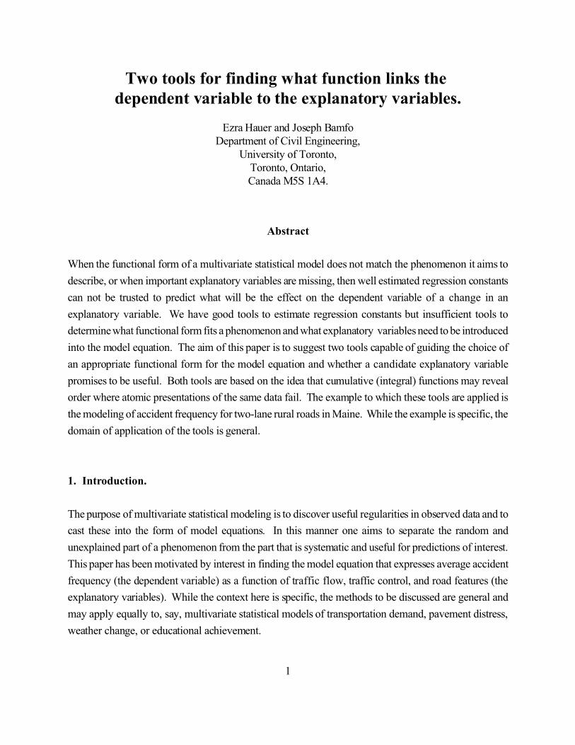
Figure 1. Single-vehicle accidents in three years versus annualaverage daily traffic.

recognition of regularity is difficult. The Integrate-Differentiate (ID) method described in section 2, has

been devised to facilitate the recognition regularity in exploratory data analysis. Its main idea is that

patterns are clearer when data are presented in accumulated form. The same idea is at the root of the

CURE method, for the examination of Cumulative Residuals described in section 3.

2. The Integrate-Differentiate (ID) method for recognizing a suitable functional form.

In this section, the ID method is illustrated for the one-explanatory variable case. In the

illustration, we seek the functional form relating the expected accident frequency to traffic flow. Figure

1 shows a scatterplot of accident data for 1796 rural, two-lane, 0.05 mile long, homogeneous, non-

contiguous, road sections in Maine. The abscissa of each point is the Average Annual Daily Traffic

(AADT) for the road section in three years and the ordinate is the count of single-vehicle accidents

recorded on that road section in

the same three-year period. A

grand total of 108 single-

vehicle accidents occurred on

these nearly 90 miles of road

sections in three years. The

vast majority of road sections

had no accidents, some had

one, and a few recorded two

accidents. If there is some

systematic association between

traffic flow and average

accident frequency, it is

certainly not discernible in

Figure 1.

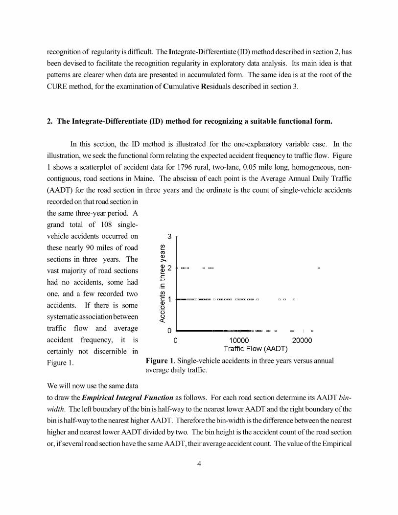
We will now use the same data

to draw the Empirical Integral Function as follows. For each road section determine its AADT bin-

width. The left boundary of the bin is half-way to the nearest lower AADT and the right boundary of the

bin is half-way to the nearest higher AADT. Therefore the bin-width is the difference between the nearest

higher and nearest lower AADT divided by two. The bin height is the accident count of the road section

or, if several road section have the same AADT, their average accident count. The value of the Empirical

5

Figure 2. The Empirical Integral Function for the data in Figure 1.

Integral Function at the right boundary of the bin is the sum of all bin areas from the lowest AADT up

to that boundary. The Empirical Integral Function, for the data in Figure 1 is shown in Figure 2. It is

evident that the apparently patternless data in Figure 1 have been rearranged so as to reveal some order.

To explain the essence of Figure 2, assume that there exists a function 6=f(x) linking the expected

accident frequency, 6, and the Annual Average Daily Traffic, x. The definite integral of f(x) from x=0

to x=X, i.e., the area under the curve f(x), will be called the Integral Function, F(X). The summation

of bin areas which gave rise to the Empirical Integral Function, to be denoted by FE(X), is an estimate

of the same area. Thus, the FE(X) is an estimate of F(X). If the functional form of F(X) can be recognized

by examining the Empirical Integral Function FE(X), then the functional form of f(x) follows as the

derivative of F(X). The main idea of the ID method is that one can fruitfully speculate about the

functional form behind the Empirical Integral Function even when the scatterplot shows no discernible

pattern. Graphical illustrations of some candidate f(x) that may link accidents and traffic flow, and the

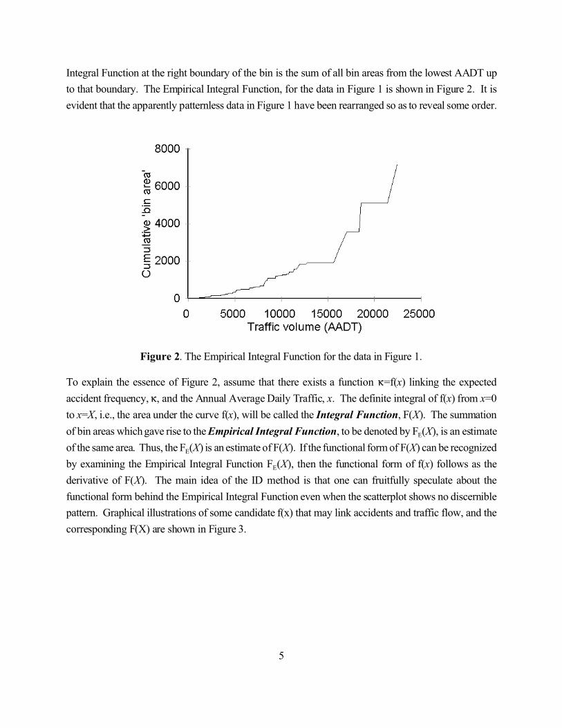
corresponding F(X) are shown in Figure 3.

6

Power function: f1(x)="x$ Power Function: F1(X)=["/($+1)]X$+1

Polynomial function: f2(x)="x+$x2 Polynomial function:F2(X)=("/2)X2+($/3)X3

Hoerl’s function: f3(x)="xe$x Hoerl’s function: F3(X)="[e$X($X-1)/$2 +1/$2]

Figure 3: Corresponding f(x) and F(X).

The order created by the cumulation of bin areas may be partly illusory since many cumulative curves

look similar. Only functions with constantly increasing slope and those with a point of inflection can be

7

Figure 4: Does the transformed F1 fit a straight line?

Figure 5: Does the transformed F2 fit a straight line?

distinguished. However, some discernment is possible. Thus, for instance, were the expected accident

frequency 6 a constant that does not depend on AADT, then F(X) would be a straight line through the

origin. This is surely not the case here. Were 6=f1(x)="x$ then, as shown in Figure 3, this is a candidate

function for the Empirical integral Function in Figure 2, but only if $>0. Were f2(x)="x+$x2 then

F2(X)=("/2)X2+($/3)X3. This functional form can reproduce a point of inflection when $<0. However,

since no decrease in slope is indicated in Figure 2, $>0 seems appropriate here. One might also entertain

Hoerl’s function but it also must show no point of inflection within the range of AADTs. This is probably

the farthest that discernment by inspection of the Empirical Integral Function can go in this case.

Whether F1 or F2 fit the data better can be determined relatively simply. If F1 is suitable, then plotting

log[FE(X)]) against log(X) one should see a straight line with log["/($+1)] as intercept and $+1 as slope.

Similarly, if F2 is suitable, then plotting FE(X)/X2 against X should yield a straight line with the intercept

"/2 and slope $/3. The two plots are shown as Figures 4 and 5.

It appears that the power function F1 will fit the data well for AADT$700 [log(700)=6.5]. The cubic

function F2 does not seem to fit the data well for AADT<5000 or so. Thus, while neither one of the two

identified candidate functional forms promises to be a good fit over the entire range of the variable

AADT, the power function seems to be the more suitable of the two. There exist, of course, many other

candidate functional forms. If their F(X) can not be easily transformed into a linear form there is probably

no better option than to estimate their regression constants by the usual means and then to examine their

residuals by the method described in Section 3.

8

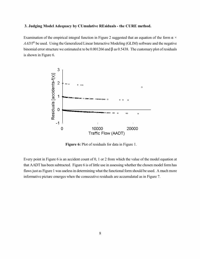
Figure 6: Plot of residuals for data in Figure 1.

3. Judging Model Adequacy by CUmulative REsiduals - the CURE method.

Examination of the empirical integral function in Figure 2 suggested that an equation of the form " ×

AADT$ be used. Using the Generalized Linear Interactive Modeling (GLIM) software and the negative

binomial error structure we estimated " to be 0.001266 and $ as 0.5438. The customary plot of residuals

is shown in Figure 6.

Every point in Figure 6 is an accident count of 0, 1 or 2 from which the value of the model equation at

that AADT has been subtracted. Figure 6 is of little use in assessing whether the chosen model form has

flaws just as Figure 1 was useless in determining what the functional form should be used. A much more

informative picture emerges when the consecutive residuals are accumulated as in Figure 7.

9

Figure 7: Plot of cumulative residuals for data in Figure 1.

If a model equation fits the data along the entire range of values assumed by a variable, one expects the

cumulative graph to be a random walk oscillating around 0. Furthermore, depending somewhat on the

principle used for regression constant estimation, one expects this random walk to end close to 0. The

question arises, whether a cumulative graph of the kind shown in Figure 7 is a sign that the model is

flawed for some ranges of the variable, or whether it is compatible with a random walk of a model fitting

over the entire range of the variable, such that the mean of all residuals is 0.

The graph in Figure 7 indeed oscillates around 0. When along a stretch of the horizontal axis the

cumulative residuals consistently drift upwards, there are more accidents there then what the model

predicts. Conversely, when the cumulative residuals consistently drift down, the model overestimates the

accident count. Thus, for example, from point A at which the residuals accumulate to about +6 (after 1123

road sections at AADT�1300) to point B at which the residuals accumulate to about -8 (at road section

1535 and AADT�4200), the model seems to overestimate the accident counts. Similarly from point B

on, the estimates produced by this model form seem to be consistently too small. Since a grand total of

108 accidents occurred on these road sections in the three years, it is difficult to judge whether such peak

accumulations (+6, -8) are a sign of a poor fit. Some formal tool is needed to distinguish between what

may be expected if the model fits perfectly and what is a sign of a systematic bias.

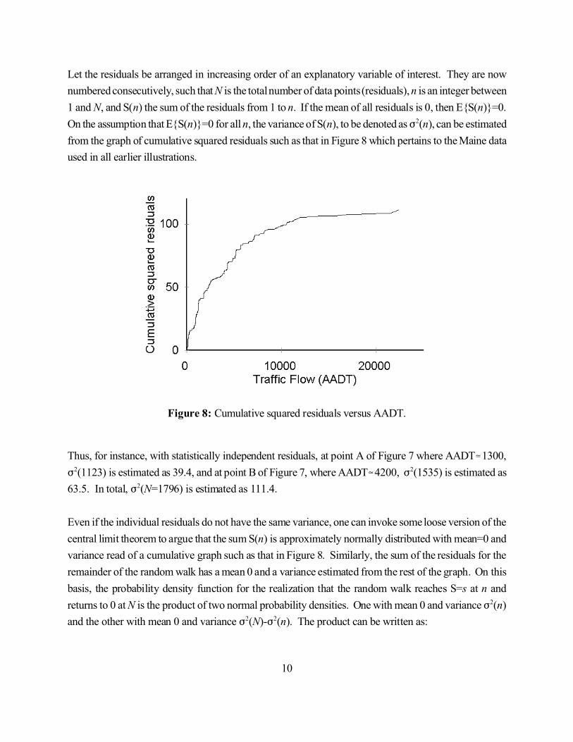
10

Figure 8: Cumulative squared residuals versus AADT.

Let the residuals be arranged in increasing order of an explanatory variable of interest. They are now

numbered consecutively, such that N is the total number of data points (residuals), n is an integer between

1 and N, and S(n) the sum of the residuals from 1 to n. If the mean of all residuals is 0, then E{S(n)}=0.

On the assumption that E{S(n)}=0 for all n, the variance of S(n), to be denoted as F2(n), can be estimated

from the graph of cumulative squared residuals such as that in Figure 8 which pertains to the Maine data

used in all earlier illustrations.

Thus, for instance, with statistically independent residuals, at point A of Figure 7 where AADT�1300,

F2(1123) is estimated as 39.4, and at point B of Figure 7, where AADT�4200, F2(1535) is estimated as

63.5. In total, F2(N=1796) is estimated as 111.4.

Even if the individual residuals do not have the same variance, one can invoke some loose version of the

central limit theorem to argue that the sum S(n) is approximately normally distributed with mean=0 and

variance read of a cumulative graph such as that in Figure 8. Similarly, the sum of the residuals for the

remainder of the random walk has a mean 0 and a variance estimated from the rest of the graph. On this

basis, the probability density function for the realization that the random walk reaches S=s at n and

returns to 0 at N is the product of two normal probability densities. One with mean 0 and variance F2(n)

and the other with mean 0 and variance F2(N)-F2(n). The product can be written as:

11

(1)

(2)

(3)

(4)

The part of equation (1) with the exponents can be rewritten as

with,

The remaining part of equation (1) can be rewritten as

Thus, the product in equation (1) represents a normal probability density with mean 0 and standard

deviation F* that is multiplied by the constant 1//[2BF(N)]. Therefore, the probability density for a

random walk that ends at 0 to pass through S(n)=s is normal with a mean of 0 and variance F*2=F2(n)[1-

F2(n)/F2(N)].

In the numerical example, F2(1123) was estimated to be 39.4 and F2(1796) was estimated as 111.5. Thus

F*2=39.4(1-39.4/111.4)=25.5 and F*=5.1. Recall that the observed S(1123) was about 6. That is slightly

more than one standard deviations from the mean and entirely compatible with the hypothesis that the

model residuals are 0 everywhere. Similarly at n=1535 where S(1535) is about -8, F*2=63.5(1-

63.5/111.4)=27.3 and F*=5.2. Since -8/5.2<2 the random walk at its extremes is contained within two

standard deviations of what would be expected if the fit was perfect. Since F* varies with n and is 0 near

the edges, it is perhaps best to examine the entire plot of 2F* against the background of the cumulative

residuals is shown in Figure 9.

12

Figure 9: Cumulative residuals and the ±2F* band.

Recall that the plot of cumulative squared residuals (such as that in Figure 8) estimates F2(n) on the

assumption that E{S(n)}=0. This will almost never be exactly true. If so, the plot of cumulative squared

residuals will contain some bias and F2(n) is in truth less than the value of the cumulative squared residual

at n. As a result the ±2F*(n) band such as that shown in Figure 9 is somewhat wider than it should be.

In conclusion, the functional form chosen in the illustration seems to produce estimates of 6 that are

slightly too high for 1300<AADT<4200 and slightly too small for AADT>4200. It is possible that a

different model functional form, one that shapes the curve in accord with these observations, can be

found. Thus, for example, the model 0.003466 × AADT0.3721 × e0.000072 × AADT will produce a better

cumulative residual plot. However, inasmuch as the cumulative residuals in Figure 9 are not inconsistent

with the hypothesis that all expected residuals are 0, we adopt tentatively, for the explanatory variable

"AADT", the simpler form, 0.001266 × AADT0.5438.

The purpose of this section was to show that when data are noisy and the plot of residuals against some

variable is uninformative (as is, e.g., Figure 6), the plot of cumulative residuals may still be interpretable

and useful. The very same CURE technique is useful also when one wishes to ascertain whether a new

explanatory variable should be introduced into the model equation. Produce the graph of cumulative

residuals against the candidate explanatory variable. Using the cumulative squared residuals, when

arranged in the order of the new explanatory variable, estimate the F*(n). If the graph of cumulative

13

residuals oscillates around 0, ends near 0, and is confined within, say, ±2F*(n), the new explanatory

variable will not be useful.

In the numerical illustrations so far, we used only traffic volume (AADT) as an explanatory variable.

Road section length was kept constant at 0.05 miles. Next we will introduce road section length as the

additional explanatory variable. It is not really necessary to use the CURE technique to determine

whether road section length needs to be added to the model equation. In fact, one may think, a-priory,

that 6 should be proportional to road section length. However, since some researchers found to the

contrary, an empirical examination is in order. More generally, the discussion so far has been confined

to the case when 6 is a function of one variable only. In the next section we illustrate the application of

the ID approach to the case when the model equation contains several explanatory variables.

4. Generalization to more than one explanatory variable.

Consider a model equation of the form 6=f1(x1)f2(x2) and assume that the functional form and regression

constants of f1(x1) are known. We wish to ascertain the functional form of f2(x2). In Section 2, where 6

was considered to be a function of only one variable, we made use of the Empirical Integral Function of

6. The idea here is to use the Empirical Integral Function of the ratio, 6/f1(x1), considering provisionally

f1(x1) as known.

To illustrate, let the road section length d be the argument of f2. On logical grounds we expect f2(d) to

be as straight line through the origin. The reason is that if we divide a homogeneous road section into

two segments, we expect the number of accidents on the original road section to be the sum of the number

expected on the two segments.

As earlier, when constructing the empirical integral function for AADT, we need to determine the bin

widths and bin heights for the data. Our data now is about 40,753 two-lane, rural road sections in Maine

that vary in length from 0.01 miles to 4.89 miles. (In the preceding sections we used a subset of these

consisting of 1796 road sections that are 0.05 miles long.) Of the 489 possible values of d, 341 are

actually represented in the data. Bin width will be determined, as before, by the difference between the

nearest higher and nearest lower road section length divided by two. As bin height we will use the ratio:

(count of accidents for all the road sections in bin)/(number of accidents predicted by " × AADT$ for all

the road sections in the bin). These are the ordinates in Figure 10.

14

Figure 10: Bin width versus road section length.

In this case it may seem that further inquiry is not needed. The reliably determined points (say, those for

d<1.3 miles where each bin contains more than 100 accidents) clearly chart a straight line through the

origin. Thus, we find what should hold true, namely, that f2(d) is a straight line through the origin. It is

tempting to conclude that the same relationship holds also beyond, say, d>2 miles. However, since here

the points could admit many functional forms, the Empirical Integral Function could again be useful. It

is shown in Figure 11.

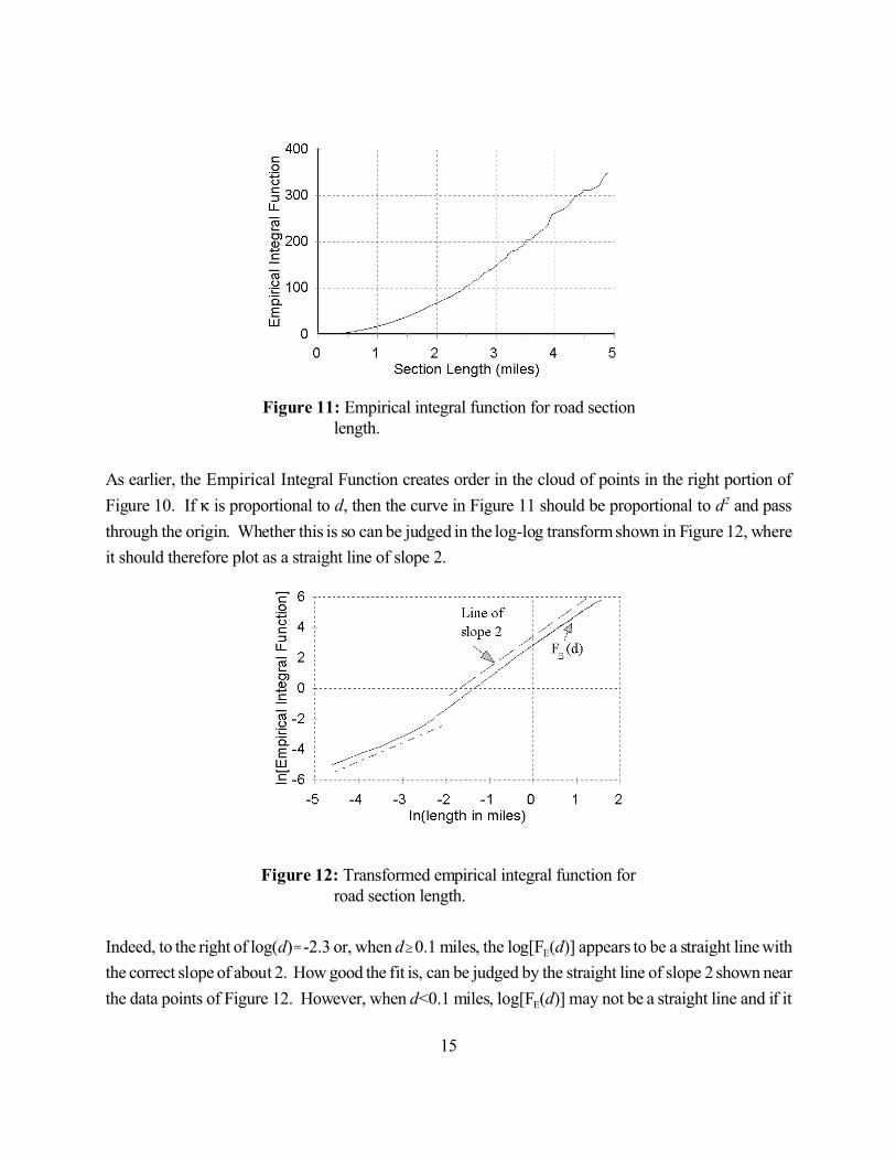
15

Figure 11: Empirical integral function for road section length.

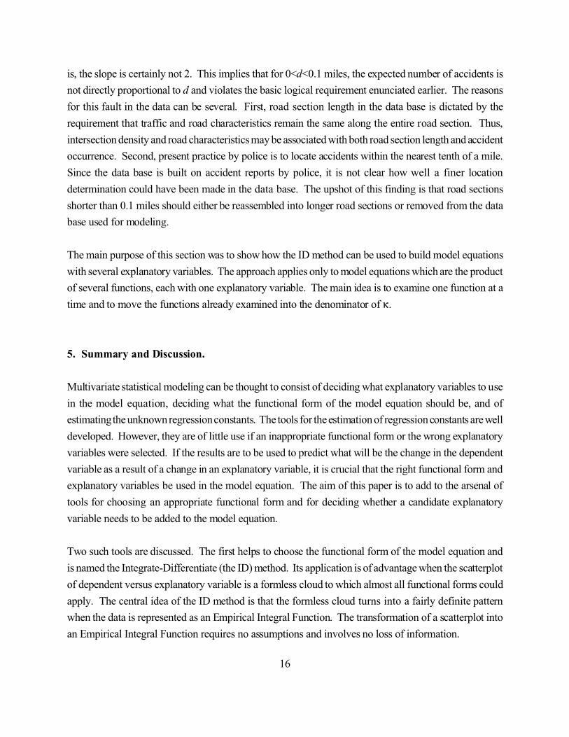
Figure 12: Transformed empirical integral function for road section length.

As earlier, the Empirical Integral Function creates order in the cloud of points in the right portion of

Figure 10. If 6 is proportional to d, then the curve in Figure 11 should be proportional to d2 and pass

through the origin. Whether this is so can be judged in the log-log transform shown in Figure 12, where

it should therefore plot as a straight line of slope 2.

Indeed, to the right of log(d)�-2.3 or, when d$0.1 miles, the log[FE(d)] appears to be a straight line with

the correct slope of about 2. How good the fit is, can be judged by the straight line of slope 2 shown near

the data points of Figure 12. However, when d<0.1 miles, log[FE(d)] may not be a straight line and if it

16

is, the slope is certainly not 2. This implies that for 0<d<0.1 miles, the expected number of accidents is

not directly proportional to d and violates the basic logical requirement enunciated earlier. The reasons

for this fault in the data can be several. First, road section length in the data base is dictated by the

requirement that traffic and road characteristics remain the same along the entire road section. Thus,

intersection density and road characteristics may be associated with both road section length and accident

occurrence. Second, present practice by police is to locate accidents within the nearest tenth of a mile.

Since the data base is built on accident reports by police, it is not clear how well a finer location

determination could have been made in the data base. The upshot of this finding is that road sections

shorter than 0.1 miles should either be reassembled into longer road sections or removed from the data

base used for modeling.

The main purpose of this section was to show how the ID method can be used to build model equations

with several explanatory variables. The approach applies only to model equations which are the product

of several functions, each with one explanatory variable. The main idea is to examine one function at a

time and to move the functions already examined into the denominator of 6.

5. Summary and Discussion.

Multivariate statistical modeling can be thought to consist of deciding what explanatory variables to use

in the model equation, deciding what the functional form of the model equation should be, and of

estimating the unknown regression constants. The tools for the estimation of regression constants are well

developed. However, they are of little use if an inappropriate functional form or the wrong explanatory

variables were selected. If the results are to be used to predict what will be the change in the dependent

variable as a result of a change in an explanatory variable, it is crucial that the right functional form and

explanatory variables be used in the model equation. The aim of this paper is to add to the arsenal of

tools for choosing an appropriate functional form and for deciding whether a candidate explanatory

variable needs to be added to the model equation.

Two such tools are discussed. The first helps to choose the functional form of the model equation and

is named the Integrate-Differentiate (the ID) method. Its application is of advantage when the scatterplot

of dependent versus explanatory variable is a formless cloud to which almost all functional forms could

apply. The central idea of the ID method is that the formless cloud turns into a fairly definite pattern

when the data is represented as an Empirical Integral Function. The transformation of a scatterplot into

an Empirical Integral Function requires no assumptions and involves no loss of information.

17

The use and usefulness of the ID method has been demonstrated on data about single-vehicle non-

intersection accidents on rural two-lane roads in Maine. In one instance of application, it proved possible

to first identify the power function of traffic flow and the parabola as candidate functional forms, and then

to determine that the power function is the more suitable candidate of the two. In the next instance of

application, the ID method was used to determine the functional form in which the explanatory variable

‘road section length’ should enter the model equation. Not only could we confirm that what is logically

sound is strongly supported by data, we could also demonstrate that for road sections shorter than 0.1

miles the logical relationship is violated and concluded that such road sections must not be used in

modeling.

The ID method, as presented, applies only to functional forms that are products of functions of one

variable (i.e., f1(x1) × f2(x2) ×. . .). Whether it can be extended to more general functional forms,

considering two or more explanatory variables at once, requires further inquiry. As explained, the ID

method is not an automatic procedure. It requires that the analyst examine each explanatory variable

separately, with the model equation evolving one explanatory variable at a time, and with the need to

occasionally revisit the functional form of variables already examined.

The second tool discussed in this paper, the CURE method, is tied to the examination of residuals after

regression constants were estimated. Its purpose is twofold. First, it can be used to examine whether the

chosen functional form indeed fits the explanatory variable along the entire range of its values represented

in the data. If not, it informs the search for a better functional form. Second, it can also be used to

ascertain whether a candidate explanatory variable, one not yet used, should be introduced into the model

equation. The central idea is that even when the usual plot of residuals does not show any systematic

drift, by examining the cumulative residuals, potentially important patterns may emerge.

The plot of cumulative residuals should oscillate around 0, end close to 0, and not exceed the ±2F*

bounds determined by equation 2. Even if these bounds are not infringed upon but there are long

stretches where the model consistently drifts up or down, consideration can be given to improving the

model form. When the residual is defined as the difference between the accident count and the model

prediction, an upward drift is a sign that the model consistently predicts fewer accidents than were

counted. Of course, if the endpoint is not near 0, there is something wrong with the estimated regression

constants.

The two tools discussed in this paper require a cyclical process of multivariate statistical modeling, one

in which the functional form evolves gradually, its regression constants are periodically re-estimated and

18

the cumulative residuals used to both revise the functional form to try out new explanatory variables. It

is our prejudice to think that the need for a cyclical process is a useful feature of the suggested tools.