two-stage optimization method for power loss and...

Turk J Elec Eng & Comp Sci

(2018) 26: 501 – 517

c⃝ TUBITAK

doi:10.3906/elk-1602-65

Turkish Journal of Electrical Engineering & Computer Sciences

http :// journa l s . tub i tak .gov . t r/e lektr ik/

Research Article

Two-stage optimization method for power loss and voltage profile control in

distribution systems with DGs and EVs using stochastic second-order cone

programming

Huiling TANG1,2, Jiekang WU1,∗, Zhijiang WU3, Lingmin CHEN1

1School of Automation, Guangdong University of Technology, Guangzhou, P.R. China2School of Physics & Optoelectronic Engineering, Guangdong University of Technology, Guangzhou, P.R. China

3South China National Centre of Metrology, Guangzhou, P.R. China

Received: 05.02.2016 • Accepted/Published Online: 15.11.2017 • Final Version: 26.01.2018

Abstract: This paper introduces a stochastic second-order cone programming (SSCOP) approach to solve the distributed

generation coordination problem considering the uncertainty of electric vehicle charging in distribution networks. To

minimize the total power loss in the distribution system, the problem is formulated to coordinate the output power

of distributed generations (DGs). Two stages are presented to solve the optimization problem: the first stage is to

optimize the output power of distributed generators without electric vehicle charging in the distribution system, and the

second stage is to optimize the output power of distributed generators according to the stochastic increased load due

to the uncertainty of electric vehicle charging. The proposed approach is tested on 69-node and 118-node large-scale

distribution systems. The simulated results demonstrate the feasibility and effectiveness of SSCOP.

Key words: Distribution systems, power loss, distributed generation, electric vehicle, stochastic second-order cone

programming

1. Introduction

Increasing concerns about greenhouse gas emissions and the energy crisis have motivated the development

of transportation electrification. Electric vehicles (EVs) are expected to play a major role in transportation

electrification. The cumulative sales of EVs are expected to reach 5 million units by 2020 in China [1]. However,

the uncertainty of EV charging has a great impact in the distribution systems, including increasing power loss

of distribution systems and nodal voltage offset. It is necessary to develop renewable energy such as wind- and

solar-based generation units. The generation units are called distributed generations in the distribution systems

to meet the EV random load. It is also necessary to coordinate distributed generations and EVs because of

uncertainties of charging power of EVs.

Stochastic second-order cone programming with recourse is a class of optimization problems defined to

formulate many applications of DSOCP with uncertain data [2]. Second-order cone programming is a special

convex programming model [3], and is one of the important optimization methods in mathematics. The method

has been applied in power systems [4,5]. Many scholars have applied cone programming to power flow calculation

of power systems. A nonlinear constraint condition is transformed into linear in power flow calculations. The

relationship between the cone sets of variables is preserved to improve the calculation speed. For example, a

∗Correspondence: [email protected]

501

TANG et al./Turk J Elec Eng & Comp Sci

power flow calculation model is proposed based on conic programming [6]. A cone programming model for DGs

is obtained by minimizing power loss as the objective function [7]. The cone programming model for optimal

reconfiguration of the distribution network is solved by taking the switch in the lines as variables [8]. The

optimal power flow model based on second-order cone programming is established using an objective function

of minimizing active power loss, reactive power loss, and generation cost [9]. In fact, the operating conditions

of the power network are always changing, and the above literature fails to consider the impact of various

uncertainties on the power grid.

The charging power of the EV is random as the stochastic load of the distribution network. In this paper,

the uncertainty of EV charging on the electric network is studied. A stochastic second-order cone programming

(SSCOP)-based method is also presented to optimize the output of DGs in order to decrease the power loss and

the nodal voltage offset, which will bring great potential risk to the distribution system.

2. Output power of DGs and charging power of EVs

2.1. The stochastic model of solar photovoltaic power generation

Solar irradiation is a random process in a day. That is to say, solar radiation will have different values in

different time periods of a day. From the statistical analysis of historical data, solar radiation is subject to beta

distribution, and the solar radiation value always corresponds to a probability. In mathematics, the probability

density function of solar radiation can be expressed by beta distribution [10]:

f(si(t)) =

Γ(α+β)Γ(α)Γ(β) [si(t)]

α−1(1− si(t))β−1 for

0 ≤ si(t) ≤ 1α ≥ 0, β ≥ 0

0, (1)

where f(si(t)) is the beta function of the solar irradiance value si(t) at time period t , si(t) is solar irradiance

value,α and β are the parameters of the beta function, which is determined by historical irradiance data, and

Γ() is expressed as the beta function.

Although solar radiation has a different value at each time of day, the solar radiation in a certain period

of time can be considered as constant, if the solar irradiance value is supposed to be constant at each time

period. The probability of the solar irradiance value may be formulated as [10]

pS(t) =

∫ t

0

f (si (t))si (t) dt (2)

Because of the fluctuation in solar radiation in the beta distribution, the output power of a photovoltaic

power generation system is also changed according to the beta distribution in different solar radiation conditions.

If the solar radiation is changed in a certain range with the probability of beta distribution, the output power

of the photovoltaic power generation system also changes with the probability of beta distribution in a certain

range. Therefore, the output power of distributed photovoltaic generation system i at time period t may be

formulated by

PPV i(t) = ηPV iPSi(t)pS(t), (3)

where PSi(t) is the solar irradiance power of distributed photovoltaic power generation system i at time period

t , and ηPV i is the generation efficiency of distributed photovoltaic power generation system i due to the impact

of photovoltaic power generation materials on the process and results of photoelectric conversion. Obviously

502


the output power of distributed photovoltaic generation PPV i(t) is stochastic because the solar irradiance value

si(t) is stochastic at different time t .

2.2. The stochastic model of distributed wind power generation

It has been demonstrated by a large number of experiments that the stochastic wind speed in most regions

approximately follows Weibull distribution, which can be formulated as follows [11]:

f(v) =k

ckv(k−1) exp(−v

c)k 0 ≤ v ≤ ∞, (4)

where v is wind speed, and k and c are respectively the shape index and the scale index of the Weibull

distribution.

The output power level depends on the wind speed, and the output power is zero when the wind speed

is smaller than the cut-in wind speed or not less than the cut-out wind speed. When the wind speed is not less

than the cut-in wind speed and not greater than the rated wind speed, the output power increases linearly with

the wind speed. When the wind speed is not less than the rated wind speed and less than the cut-out wind

speed, the power output is in accordance with the rated power. From the statistical analysis of historical data,

it is found that the level of each output power from zero to the rated power is corresponding to a probability

value of the Weibull distribution. Therefore, the probability of the wind speed value may be formulated by [12]

pW (t) =

∫ t

0

f (vi (t))vi (t) dt, (5)

where f(vi(t)) is the Weibull function of the wind speed value vi(t) at time period t , and vi(t) is wind speed

value.

The output power of distributed wind power generation system i at time period t may be formulated by

PWi(t) = ηWiPWS(t)pW (t), (6)

where PWS(t) is wind power under wind speed of vi(t), and ηWi is generation efficiency of distributed wind

power generation system i under wind speed of vi(t). Similarly, the output power of distributed photovoltaic

generation PPV i(t) is stochastic because the wind speed value vi(t) is stochastic at different time t .

2.3. Stochastic nature of EV load

The main influencing factors of the total EV charging power in the distribution network are determined by

state of charge (SOC), the daily mileage, the recharging time of EVs, and charging time length of EVs. Due

to differences in people’s travel habits and the different characteristics of the EV’s battery, there are a lot of

uncertainties in the charging of EVs in the distribution network. Generally, the recharging power in a charging

station always is uncertain due to uncertainties of SOC in the battery, the expected traveling distance, the

recharging time, and so on. It is clear that EV charging is a random event, with a large uncertainty, and its

charging power is a random variable. The probability density functions (PDFs) of an EV’s daily mileage can

be expressed as follows [13]:

f(d) =1√

2πdσd

exp[− (ln d− µd)2

2σ2d

], (7)

503


where d is the daily distance driven by a vehicle, µd is the mean of the distribution, and σd is the standard

deviation of the probability function.

Because of differences in people’s travel habits and pattern of vehicle usage, not all EVs in the distribution

system start charging simultaneously, and so the time of switching on an individual charger is a random variable,

and the probability density functions of the battery recharging start time ts can be expressed as follows [14]:

f(ts) =1√

2πσts

exp[− (ts − µts)2

2σ2ts

], (8)

where ts is the recharging time of an EV, µts the mean, indicating the location of maximum probability density,

and σ2ts is the standard deviation of recharging time of an EV in a day.

On the other hand, assuming the SOC of an EV drops linearly with the distance of travel, the SOC at

the beginning of recharge cycle can be expressed as follows [15]:

Ei = 1− d

L, (9)

where d is the daily distance traveled by a vehicle, Ei represents the initial SOC of an EV battery, and L is

the maximum range of the EV.

The probability distribution of initial battery SOC can be expressed as (10), which is derived from (7)

and (9):

f(E) =1√

2πL(1− E)σd

exp− [ln(1− E)L− µd]2

2σ2d

(10)

The probability density function of recharging power is obtained:

p(E) =1√

2πL(1− E)tEσd

exp− [ln(1− E)L− µd]2

2σ2d

, (11)

where tE is the charging time length of EVs.

The probability density function of a battery charging load operating at power level Pj at time instant

t can be represented as ξ(Pj,t) [15]:

ξ(Pj,t) =t∑

k=1

f(ts)f(Ej−(t−k)) k ≤ t, 1 ≤ k ≤ 24 (12)

Eq. (13) then gives the expression of multiple batteries’ charging loads in the distribution system at time instant

t at node i .

PEV i,t =

ni∑m=1

NT∑j=1

Pmj .ξ(Pmj,t), (13)

where ni is the total number of EVs at node i , NT is the total number of hours of battery to be fully charged

from a fully discharged state, and Pmj is the discrete power demand value of the m-th EV at charging power

level Pj , which can be expressed as follows:

Pmj =Pm,j−1 + Pm,j

2j = 1, 2, · · ·NT (14)

504


Based on the above analysis, it is shown that the total EVs’ charging loads PEV i,t at node i in a distribution

system is a stochastic load, which is influenced by the daily mileages and vehicle traffic patterns (usage).

3. Mathematical model

3.1. Objective functions

It is assumed that a distribution system is installed with the DG of renewable energy systems and charging

systems for EVs at different nodes in this paper. Figure 1 is the single radiation line model in the distribution

system with DGs and EVs. In the system, it is also assumed that the DG of renewable energy systems includes a

DG system and a distributed energy storage system (DS). The DG system is based on solar power, wind power,

etc. The output power of the DG of a renewable energy system is dependent on the output power of the DG

system, the storage power of the energy storage system, and the load power at the local node. The renewable

energy is fully utilized by the local load, and the surplus power will be stored in the DSs when the power of

the local load is smaller than that generated from the renewable energy DG system. With this assumption,

controlling the output power of the DG means controlling the power output of renewable energy systems, and

controlling the power output of renewable energy systems means the controlled power of the renewable energy

is used for local storage. Controlling the renewable energy aims at minimizing system loss.

Figure 1. A simplified 2-node distribution system with DGs and EVs.

In the distribution system, Sij is the power flow from node i to j.SDGi or SDGj is a flow-in power

injected by the DG of renewable energy systems at node i or j.SDi or SDj is a flow-out power outpoured

by local general load at node i or j , which is uncontrollable at any time; SEV i or SEV j is a flow-out power

outpoured by changing load of EVs, which is a stochastic load.

The objective function in this paper is to minimize the power loss, which can be expressed as follows:

minT∑

t=1

[∑

(ij)∈Ωl

PLoss(Vi,t;Vj,t; θij,t)] (15)

∑(i,j)∈ΩL

PLoss(Vi,t;Vj,t; θij,t) =∑

(i,j)∈ΩL

Gij(V2i,t + V 2

j,t − 2Vi,tVj,t cos θij,t) =N∑i=1

(PDGi,t − PDi,t − PEV i,t), (16)

where Vi and Vj are the voltage magnitude of node i and j , θij is the voltage angle between node iand j ,

and ΩL is a nodal set in the distribution network. T is the study period. N is the number of nodes in the

505


distribution system and PDGi,t is real power produced by the DG of renewable energy system at node i at time

instant t.PDi,t is real power load demand at node i at time instant t.PEV i,t is the overall real power demand

for the all EV battery chargers at node i at time instant t , which is modeled as random variables across time

from a probability density function. The control task is to minimize the total power loss by properly setting

the control variables all day. The constraints associated with the above objective consist of the following.

1) Equal constraint condition∑j∈Ωi

(GijV2i,t − Vi,tVj,t(Gij cos θij,t −Bij sin θij,t)) = PDGi,t − PDi,t − PEV i,t (17)

∑j∈Ωi

(BijV2i,t − Vi,tVj,t(Bij cos θij,t +Gij sin θij,t)) = QDGi,t −QDi,t −QEV i,t (18)

Power flow as equal constraint condition must satisfy Eqs. (16) and (17).Ωi is the nodal set connected to

node i .

2) Nodal voltage constraint

As for each node in the distribution systems, its voltage must be not greater than its maximal limit and

not less than its minimal limit:Vi,min ≤ Vi,t ≤ Vi,max, (19)

where Vi , Vi,max , and Vi,min are respectively the actual value, the maximal limit, and the minimal limit

of nodal voltage at node i .

3) Branch current constraint

Current magnitude of each branch must lie within their permission ranges:

I2ij,t = (G2ij +B2

ij)(V2i,t + V 2

j,t − 2Vi,tVj,t cos θij,t) ≤ I2ij,max, (20)

where Iij,max is the maximal limit of the branch Lij .

4) Power output constraint for DG

0 ≤√(PDGi,t)2 + (QDGi,t)2 ≤ SDGi,max, (21)

where SDGi,max is the maximal power limit of the DG of the renewable energy system at node i .

3.2. Stochastic second-order cone programming for the problem

In this section we will formulate the power loss and voltage profile control in distribution systems with stochastic

charging power of EV problem presented in the previous section as a stochastic second-order cone SSOCP

problem. Stochastic second-order cone programming with recourse is a class of optimization problems defined

to handle uncertainty in data defining deterministic second-order cone programming [2]. The standard form of

stochastic second-order cone programming is the following:

minimize cTx+

ζ∑k=1

Q(k)(x) subject to Ax− b≻r10, (22)

506


where r1 ≥ 1 and r2 ≥ 1 are integersi = 1, 2, ..., r1 and j = 1, 2, ..., r2 .A ∈ Rm1×n1 ,b ∈ Rm1 , and c ∈ Rn1

are the deterministic data, x ∈ Rm1 is the first-stage decision variable, and for k = 1, 2, 3, ...ζ , ζ is the number

of realizations. Q(k)(x) is the minimum value of the problem

minimize d(k)T y(k) subject to W(k)y(k) +T(k)x− h(k)≻r20, (23)

where y(k) ∈ Rn2 is the second-stage variable, and (T(k),W(k),h(k),d(k)) are the set of the possible values of

the random variables (T(ω),W(ω),h(ω),d(ω)), where ω is underlying outcome in a finite event space Γ with

a known probability function ηk .

Likewise, the power loss and voltage profile control with stochastic charging power of EV problem given

by (15)–(21) is a problem with uncertain data. In this model, the average user load is the deterministic load

in the distribution systems, while the total power demand of EVs at every node is a stochastic load due to the

randomness of the charging power of EVs. Obviously the load of the distribution system with EVs contains

two parts. Hence the problem of power loss and voltage profile control in distribution systems with DGs and

EVs can be formulated as a two-stage programming problem. In the first stage, we optimize the output power

of the DG of renewable energy systems when there is only the deterministic load in distribution systems for

minimizing power loss and controlling voltage profile. In the second stage, we optimize the output power of the

DG of renewable energy systems when the stochastic load of charging power of EVs in the distribution system

is added.

For predicting the charging load at each time period, the continuous distribution function of the starting

charging time and the length charging time can be discretized with its discrete values Pj with 1 hour as the

unit in a day. With the notation, our two-stage stochastic programming problem can be written as

minT∑

t=1

∑(i,j)∈ΩL

PDGLoss(Vi,t;Vj,t; θij,t) +

T∑t=1

Q(t)(PDGi,t) (24)

∑(i,j)∈ΩL

PDGLoss(Vi,t;Vj,t; θij,t) =

∑(i,j)∈ΩL

Gij(V2i,t + V 2

j,t − 2Vi,tVj,t cos θij,t) =N∑i=1

(PDGi,t − PDi,t) (25)

subject to ∑j∈Ωi

(GijV2i,t − Vi,tVj,t(Gij cos θij,t −Bij sin θij,t)) = PDGi,t − PDi,t (26)

∑j∈Ωi

(BijV2i,t − Vi,tVj,t(Bij cos θij,t +Gij sin θij,t)) = QDGi,t −QDi,t (27)

Vi,min ≤ Vi,t ≤ Vi,max (28)

I2ij,t = (G2ij +B2

ij)(V2i,t + V 2

j,t − 2Vi,tVj,t cos θij,t) ≤ I2ij,max (29)

0 ≤√(PDGi,t)2 + (QDGi,t)2 ≤ SDGi,max, (30)

507


where T = 24 represents there are 24 hours in a day.PDGi,t ∈ Rn1 is the first-stage decision variable when there

is only the deterministic load in the distribution systems. Q(t)(PDGi,t) is the minimum value of the problem

min

T∑t=1

∑(i,j)∈ΩL

PDGEVLoss (V ∗

i,t;V∗j,t; θ

∗ij,t) (31)

∑(i,j)∈ΩL

PDGEVLoss (V ∗

i,t;V∗j,t; θ

∗ij,t) =

∑(i,j)∈ΩL

Gij((V∗i,t)

2 + (V ∗j,t)

2 − 2V ∗i,tV

∗j,t cos θ

∗ij,t)

=N∑i=1

(P ∗DGi,t − PDi,t − PEV i,t) (32)


(Gij(V∗i,t)

2 − V ∗i,tV

∗j,t(Gij cos θ

∗ij,t −Bij sin θ

∗ij,t)) = P ∗

DGi,t − PDi,t − PEV i,t (33)

∑j∈Ωi

(Bij(V∗i,t)

2 − V ∗i,tV

∗j,t(Bij cos θ

∗ij,t +Gij sin θ

∗ij,t)) = Q∗

DGi,t −QDi,t −QEV i,t (34)

Vi,min ≤ V ∗i,t ≤ Vi,max (35)

(I∗ij,t)2 = (G2

ij +B2ij)((V

∗i,t)

2 + (V ∗j,t)

2 − 2V ∗i,tV

∗j,t cos θ

∗ij,t) ≤ I2ij,max (36)

0 ≤√(P ∗

DGi,t)2 + (Q∗

DGi,t)2 ≤ S∗

DGi,max, (37)

where P ∗DGi,t ∈ Rn2 is the second-stage decision variable different for PDGi,t due to the uncertain load growth

of charging power of EVs with its random charging schedule. Variables with the superscript “*” are second-stage

variables.

Because the above optimization model is not the standard form of the cone programming model, it needs

to be transformed into the following form [15]:

ui,t =V 2i,t√2

or uj,t =V 2j,t√2

(38)

Hij,t = Vi,tVj,t cos θij,t Tij,t = Vi,tVj,t sin θij,t (39)

2ui,tuj,t ≥ H2ij,t + T 2

ij,t,Hij,t ≥ 0, ij ∈ ΩL (40)

Replacing variables u , H , and T in the original optimization problem with the variables of cone optimization,

a standard form of the second-order cone programming model for the original optimization problem is obtained

as (41)–(54):

minT∑

t=1

∑(i,j)∈ΩL

PDGLoss(ui,t;uj,t;Hij,t;Tij,t) +

T∑t=1

Q(t)(PDGi,t) (41)

508


∑(i,j)∈ΩL

PDGLoss(ui,t;uj,t;Hij,t;Tij,t) =

∑(i,j)∈ΩL

Gij(√2ui,t +

√2uj,t − 2Hij,t) =

N∑i=1

(PDGi,t − PDi,t) (42)


(√2Gijui,t − (GijHij,t −BijTij,t)) = PDGi,t − PDi,t (43)

∑j∈Ωi

(√2Bijui,t − (BijHij,t +GijTij,t)) = QDGi,t −QDi,t (44)

V 2i,min√2

≤ ui,t ≤V 2i,max√2

(45)

I2ij,t = (G2ij +B2

ij)(√2ui,t +

√2uj,t − 2Hij,t) ≤ I2ij,max (46)

0 ≤ P 2DGi,t +Q2

DGi,t ≤ 2 ∗ SDGi,min√2

∗ SDGi,max√2

, (47)

where SDGi,min and SDGi,max are respectively maximal and minimal power limit of the DG of the renewable

energy system at node i of the first stage. Q(t)(PDGi,t) is the minimum value of the problem

min

T∑t=1

∑(i,j)∈ΩL

PDGEVLoss (u∗

i,t;u∗j,t;H

∗ij,t;T

∗ij,t) (48)

∑(i,j)∈ΩL

PDGEVLoss (u∗

i,t;u∗j,t;H

∗ij,t;T

∗ij,t) =

∑(i,j)∈ΩL

Gij(√2u∗

i,t +√2u∗

j,t − 2H∗ij,t)

=N∑i=1

(P ∗DGi,t − PDi,t − PEV i,t) (49)


(√2Giju

∗i,t − (GijH

∗ij,t −BijT

∗ij,t)) = P ∗

DGi,t − PDi,t − PEV i,t (50)

∑j∈Ωi

(√2Biju

∗i,t − (BijH

∗ij,t +GijT

∗ij,t)) = Q∗

DGi,t −QDi,t −QEV i,t (51)

V 2i,min√2

≤ u∗i,t ≤

V 2i,max√2

(52)

(I∗ij,t)2 = (G2

ij +B2ij)(

√2u∗

i,t +√2u∗

j,t − 2H∗ij,t) ≤ I2ij,max (53)

0 ≤ (P ∗DGi,t)

2 + (Q∗DGi,t)

2 ≤ 2 ∗S∗DGi,min√

2∗S∗DGi,max√

2(54)

509


The coordination optimization of the DG and EV charging problem given by (41)–(54) is a convex optimization

problem. Interior point methods are considered to be one of the most successful classes of algorithms for

solving stochastic convex optimization problems [2]. Baha used a unified practical primal interior decomposition

algorithm to solve all SSOCP models mentioned in [2]. Thus the SSOCP models in this paper are optimized

using the second-order cone programming package MOSEK [16].

4. Simulation results of case study

The proposed solution method was implemented in MATLAB R2011b running on a Pentium Dual-core CPU,

3.06 GHz PC with 3 GB of RAM, and a 64-bit operating system. The toolbox used for optimization was

MOSEK. The code was implemented for a 69-node radial distribution system with total load of 3.802 MW+

j2.694 MVA and it is demonstrated in Figure 2. Charging stations of EVs are installed at nodes 10, 24, 32,

38, 52, and 67. From loss sensitivity factors, the top three nodes 27, 61, and 65, which are found to be more

sensitive, are chosen to install DG units in the system [17]. The DG units are solar photovoltaic and wind

turbines. The total active power of DGs is 3.6 MW and the power factor of them is 0.95. A load curve of

the 69-node distribution system is shown in Figure 3. To validate the proposed method, the code was also

implemented on a larger scale 118-node radial distribution system without tie-lines. The total power loads are

22.709MW+j17.041MVA. Detailed data of the 118-node radial distribution system are given in [18]. Charging

stations of EVs are installed at nodes 19, 44, 54, 68, 71, 78, 94, and 102 with 3000 EVs. DG units are installed

at eight nodes, 25, 36, 48, 56, 75, 88, 103, and 116, which are more sensitive to loss sensitivity factor in the

system [19]. The capacity of the DG of renewable energy systems is 1.5 MW and the power factor is 0.95. The

curve load is also shown in Figure 3 for comparability.

0 1 2 3 4 5 6 7 8 9 1011 121314151617181920212223 240

0.2

0.4

0.6

0.8

1

1.2

Hour/h

Lo

ad p

ow

er/p

.u.

Figure 2. A distribution system with 69 nodes. Figure 3. Daily load demand curve.

4.1. EV charging power

It is taken 500 EVs for the 69-node system and 3000 EVs for the 118-node as considered, which are randomly

distributed at the nodes mentioned above. The total charging power of all EVs in the 69-node system in a

day is shown in Figure 4 and that of the 118-node system is shown in Figure 5. The time period 0600–0800

is peak for people to travel out by much more EVs, and there are much fewer EVs going to charging stations

510


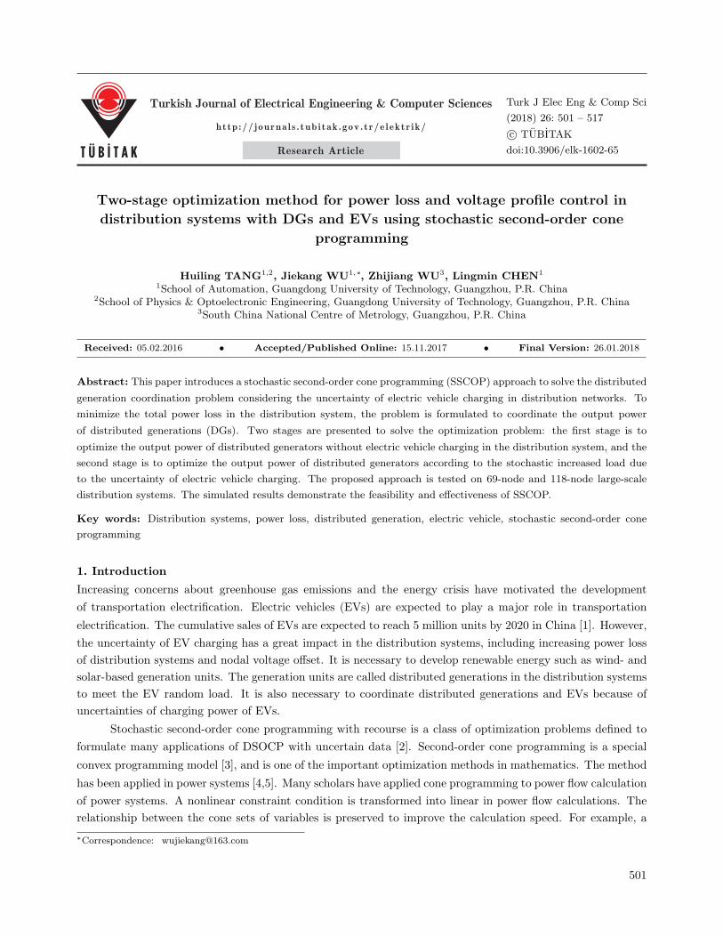
for recharging. Thus the charging power of EVs is only 0.5 MW in the 69-node system and only 0.7 MW in

the 118-node system at the time period. The number and the charging power of EVs increase with time. It

reaches maximum charging power at 2000–2200, which is the arrival time of EVs. The time period 2000–2200

is charging peak time, in which the number and the electric power of charging EVs are maximal.

0 5 10 15 20 25200

400

600

800

1000

1200

1400

1600

1800

Hour/h

Ch

argi

ng

po

wer

/P（k

W）

0 5 10 15 20 250.5

1

1.5

2

2.5

3

3.5

4

4.5

5

5.5

Hour/h

)W

M(P/re

wop gn igrahC

Figure 4. Daily curve for charging power of EVs for 69-

node system.

Figure 5. Daily curve for charging power of EVs for 118-

node system.

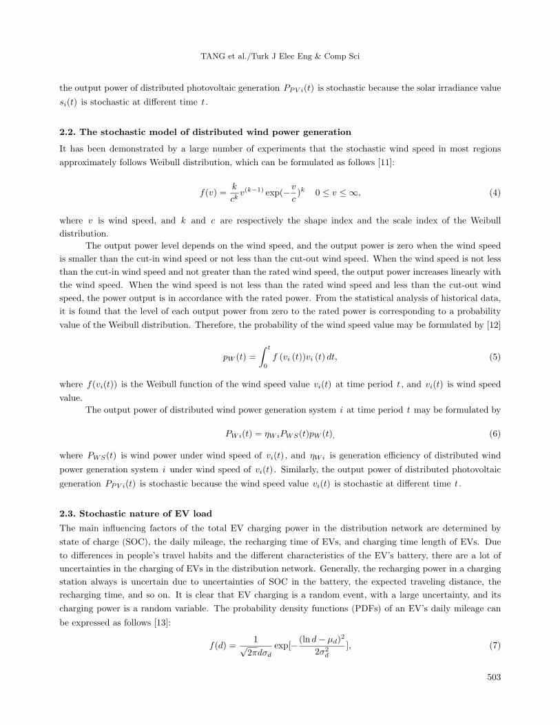
Figures 6 and 7 show respectively the 24-h power loss of the base case and that with EVs in the 69-node

system and 118-node system. Due to the stochastic charging load power of EVs the power loss with EVs is

much larger than that of the base case, which shows that the randomness of charging power of EVs has a great

impact on the power grid. The power loss may reach a very serious level especially in the EV charging peak

time 2000–2200 when the peak power of the general is added to the distribution network.

1 2 3 4 5 6 7 8 9 10 11 12 13 14 15 1617 18 19 20 21 22 23 240

0.1

0.2

0.3

0.4

0.5

0.6

0.7

0.8

0.9

1

Hour

Po

wer

loss

/MW

base case

case with EVs

1 2 3 4 5 6 7 8 9 10 11 12 13 14 15 16 17 18 19 20 21 22 23 240

0.5

1

1.5

2

2.5

3

Hour

Po

wer

loss

/MW

base case

case with EVs

Figure 6. Daily curves of system power loss with and

without EVs for 69-node system.

Figure 7. Daily curves of system power loss with and

without EVs for 118-node system.

Table 1 and Table 2 show respectively the power flow of some nodes at three specific time periods, 0600–

0800, 1400–1600, and 2000–2200, in the 69-node system and 118-node system. It can be seen from the two

511


tables that the voltage amplitudes and angles of some nodes in the network exceed the maximum allowable

value of the voltage offset and the power loss may reach a very serious level especially in the electric vehicle

charging peak time when the peak power of the general is added to the distribution network.

Table 1. Power flow of a 69-node distribution system with EVs.

Node number0600–0800 1400–1600 2000–2200

Amplitude/p.u. Angle/deg. Amplitude/p.u. Angle/deg. Amplitude/p.u. Angle/deg.

27 1.0020 0.3735 0.9973 0.4054 0.9567 0.5074

35 1.0245 0.0047 1.0437 0.0058 1.0455 0.0057

49 1.0401 -0.1536 1.0396 -0.1771 1.0379 -0.2536

41 1.0264 0.1036 1.0216 0.0969 1.0125 0.1013

53 0.9623 0.8336 0.9550 0.9418 0.9258 1.2183

54 0.9643 0.8598 0.9413 0.9643 0.9214 1.2503

69 1.0165 0.2318 1.0110 0.2432 0.9237 0.2903

Ploss/MW 0.1635 0.2192 0.4262

Table 2. Power flow of the 118-node distribution system with EVs.

Node number0600–0800 1400–1600 2000–2200

Amplitude/p.u. Angle/deg. Amplitude/p.u. Angle/deg. Amplitude/p.u. Angle/deg.

25 1.0371 –0.0423 1.0267 –0.0632 1.0189 –0.0980

47 1.0111 –0.2784 1.0008 –0.3597 0.9846 –0.5657

54 1.0009 –0.1777 0.9878 –0.2318 0.9631 –0.4065

75 0.9777 –0.0479 0.9519 –0.1391 0.9018 –0.3729

77 0.9768 –0.0318 0.9507 –0.1179 0.9001 –0.3421

85 1.0243 –0.2280 1.0169 –0.3264 1.0042 –0.5092

113 0.9982 0.6669 0.9821 0.8304 0.9574 1.0960

Ploss/MW 0.6349 1.0288 2.0122

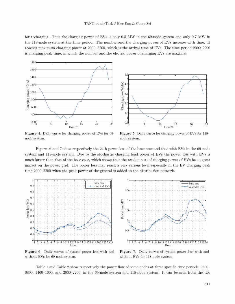
4.2. Distributed generation coordination using SSCOP

In order to reduce the impact of the randomness of charging power of EVs, it is necessary to regulate the

power output of the DG of renewable energy systems using SSOCP. Using the interior point method to solve

the problem, the optimal results of the first stage in the two distribution systems are shown in Figures 8–11,

respectively. They show that due to DGs injected the voltage offset and the power loss are smaller than that

for the base case. In the second stage the load in the distribution systems contains two parts. One is the

deterministic load; the other is the stochastic load of charging power of EVs. The optimal results of the second

stage for the 69-node system and 118-node system are shown in Figures 12–15. The optimal output power of

the DG of renewable energy systems in two different stages in the two distribution systems in the three specific

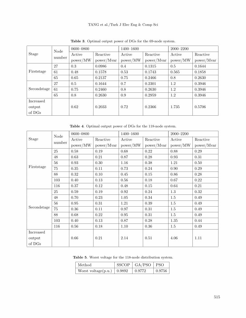
time periods is shown in Tables 3 and 4, respectively. It can be seen from Tables 3 and 4 that in the second

stage the output power of the DG of the renewable energy systems is greater than that in the first stage due to

the randomness of EVs’ charging power.

512


0 10 20 30 40 50 60 700.94

0.96

0.98

1

1.02

1.04

1.06

Bus no.

Vo

ltag

e M

agn

itu

de

(p.u

.)

base case

case with DGs

0 20 40 60 80 100 1200.95

0.96

0.97

0.98

0.99

1

1.01

1.02

1.03

1.04

1.05

Bus no.

Vo

ltag

e m

agn

itu

de(

p.u

.)

base case

case with DGs

Figure 8. First stage of nodal voltage change within

2000–2200 for 69-node system.

Figure 9. First stage of nodal voltage change within

2000–2200 for 118-node system.

1 2 3 4 5 6 7 8 9 10 11 12 13 14 15 1617 18 19 20 21 22 23 240

0.1

0.2

0.3

0.4

0.5

0.6

0.7

0.8

0.9

1

Hour

Po

wer

loss

/MW

base case

case with DGs

1 2 3 4 5 6 7 8 9 10 11 12 13 14 15 1617 18 19 20 21 22 23 240

0.5

1

1.5

2

2.5

3

Hour

Po

wer

loss

/MW

base case

case with DGs

Figure 10. First stage of daily curves for power loss of

69-node system.

Figure 11. First stage of daily curves for power loss of

118-node system.

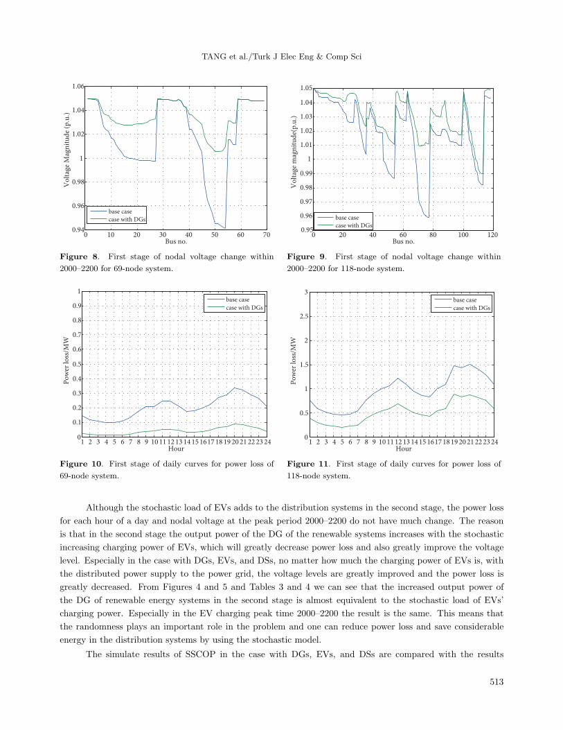
Although the stochastic load of EVs adds to the distribution systems in the second stage, the power loss

for each hour of a day and nodal voltage at the peak period 2000–2200 do not have much change. The reason

is that in the second stage the output power of the DG of the renewable systems increases with the stochastic

increasing charging power of EVs, which will greatly decrease power loss and also greatly improve the voltage

level. Especially in the case with DGs, EVs, and DSs, no matter how much the charging power of EVs is, with

the distributed power supply to the power grid, the voltage levels are greatly improved and the power loss is

greatly decreased. From Figures 4 and 5 and Tables 3 and 4 we can see that the increased output power of

the DG of renewable energy systems in the second stage is almost equivalent to the stochastic load of EVs’

charging power. Especially in the EV charging peak time 2000–2200 the result is the same. This means that

the randomness plays an important role in the problem and one can reduce power loss and save considerable

energy in the distribution systems by using the stochastic model.

The simulate results of SSCOP in the case with DGs, EVs, and DSs are compared with the results

513


0 10 20 30 40 50 60 700.94

0.96

0.98

1

1.02

1.04

1.06

Bus no.

Vo

ltag

e m

agn

itu

de

(p.u

.)

base case

case with DGs

case with DGs and EVs (SSCOP)

case with DGs, EVs, and DSs (SSCOP)

1 2 3 4 5 6 7 8 9 10 11 12 13 14 15 1617 18 19 20 21 22 23 240

0.1

0.2

0.3

0.4

0.5

0.6

0.7

0.8

0.9

1

Hour

Po

wer

lo

ss/M

W

base case

case with DGs


case with DGs, EVs, and DSs (SSCOP)

Figure 12. Second stage of nodal voltage change within

2000–2200 of 69-node system.

Figure 13. Second stage of daily curves for power loss of

69-node system.

0 20 40 60 80 100 1200.94

0.96

0.98

1

1.02

1.04

1.06

Bus no.

Vo

ltag

e m

agn

itu

de

(p.u

.)

base casecase with DGscase with DGs and EVs (SSCOP)case with DGs, EVs, and DSs (SSCOP)

1 2 3 4 5 6 7 8 9 10 11 12 13 14 15 1617 18 19 20 21 22 23 240

0.5

1

1.5

2

2.5

3

Hour

Po

wer

lo

ss/M

W

base case

case with DGs


case with DGs,EVs, and DSs (SSCOP)

Figure 14. Second stage of nodal voltage change within

2000–2200 of 118-node system.

Figure 15. Second stage of daily curves for power loss of

118-node system.

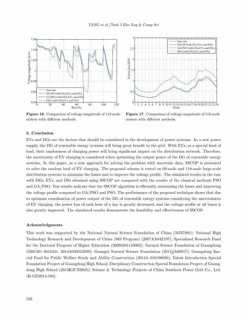
obtained by the classical methods PSO and combined GA/PSO also in the case with DGs, EVs, and DSs.

The voltage profile curves of the 118-node system with different methods are compared in Figure 16. It is

observed that the voltage magnitude simulated by SSCOP is the most highly improved compared with PSO

and combined GA/PSO. Figure 17 shows the power loss in each branch of the 118-node system simulated with

different methods. From Figure 17, it is observed that the loss at each line is highly reduced after the DG

systems’ installation at optimum locations while the proposed solution SSCOP prominently reduces the loss

at each line compared with the other two classical algorithms. Table 5 shows the methods that are compared

regarding minimum node voltage magnitude in the 118-node system.

From the above compared results, we can confirm that with the application of the SSCOP the voltage

level is improved and loss reduced compared with the results of PSO and combined GA/PSO. It also shows the

advantages of dividing the load into two stages with the SSCOP.

514


Table 3. Optimal output power of DGs for the 69-node system.

StageNode

0600–0800 1400–1600 2000–2200

Active Reactive Active Reactive Active Reactivenumber

power/MW power/Mvar power/MW power/Mvar power/MW power/Mvar

Firststage

27 0.3 0.0986 0.4 0.1315 0.5 0.1644

61 0.48 0.1578 0.53 0.1743 0.565 0.1858

65 0.65 0.2137 0.75 0.2466 0.8 0.2630

Secondstage

27 0.5 0.1644 0.7 0.2301 1.2 0.3946

61 0.75 0.2460 0.8 0.2630 1.2 0.3946

65 0.8 0.2630 0.9 0.2959 1.2 0.3946

Increased

output 0.62 0.2033 0.72 0.2366 1.735 0.5706

of DGs

Table 4. Optimal output power of DGs for the 118-node system.

StageNode

0600–0800 1400–1600 2000–2200

Active Reactive Active Reactive Active Reactivenumber

power/MW power/Mvar power/MW power/Mvar power/MW power/Mvar

Firststage

25 0.58 0.19 0.68 0.22 0.88 0.29

48 0.63 0.21 0.87 0.28 0.93 0.31

56 0.93 0.30 1.16 0.38 1.21 0.50

75 0.35 0.11 0.73 0.24 0.90 0.29

88 0.32 0.10 0.45 0.15 0.86 0.28

103 0.40 0.13 0.56 0.18 0.67 0.22

116 0.37 0.12 0.48 0.15 0.64 0.21

Secondstage

25 0.59 0.19 0.92 0.24 1.3 0.32

48 0.70 0.23 1.05 0.34 1.5 0.49

56 0.95 0.31 1.21 0.39 1.5 0.49

75 0.36 0.11 0.97 0.31 1.5 0.49

88 0.68 0.22 0.95 0.31 1.5 0.49

103 0.40 0.13 0.87 0.28 1.35 0.44

116 0.56 0.18 1.10 0.36 1.5 0.49

Increased

output 0.66 0.21 2.14 0.51 4.06 1.11

of DGs

Table 5. Worst voltage for the 118-node distribution system.

Method SSCOP GA/PSO PSO

Worst voltage(p.u.) 0.9892 0.9772 0.9756

515


0 20 40 60 80 100 1200.94

0.96

0.98

1

1.02

1.04

1.06

Bus No.

Vo

ltag

e m

agn

itu

de

(p.u

.)

base case

SSCOP (with DGs,EVs, and DSs)

GA/PSO (with DGs,EVs, and DSs)

PSO (with DGs,EVs, and DSs)

1 2 3 4 5 6 7 8 9 10 11 12 13 14 15 1617 18 19 20 21 22 23 240

0.5

1

1.5

2

2.5

3

Hour

Po

wer

lo

ss/M

W

base case

SSCOP (with DGs,EVs, and DSs)

GA/PSO (with DGs,EVs, and DSs)

PSO (with DGs,EVs, and DSs)

Figure 16. Comparison of voltage magnitude of 118-node

system with different methods.

Figure 17. Comparison of voltage magnitude of 118-node

system with different methods.

5. Conclusion

EVs and DGs are the factors that should be considered in the development of power systems. As a new power

supply, the DG of renewable energy systems will bring great benefit to the grid. With EVs, as a special kind of

load, their randomness of charging power will bring significant impact on the distribution network. Therefore,

the uncertainty of EV charging is considered when optimizing the output power of the DG of renewable energy

systems. In this paper, as a new approach for solving the problem with uncertain data, SSCOP is presented

to solve the random load of EV charging. The proposed scheme is tested on 69-node and 118-node large-scale

distribution systems to minimize the losses and to improve the voltage profile. The simulated results in the case

with DGs, EVs, and DSs obtained using SSCOP are compared with the results of the classical methods PSO

and GA/PSO. Test results indicate that the SSCOP algorithm is efficiently minimizing the losses and improving

the voltage profile compared to GA/PSO and PSO. The performance of the proposed technique shows that due

to optimum coordination of power output of the DG of renewable energy systems considering the uncertainties

of EV charging, the power loss of each hour of a day is greatly decreased, and the voltage profile at all buses is

also greatly improved. The simulated results demonstrate the feasibility and effectiveness of SSCOP.

Acknowledgments

This work was supported by the National Natural Science Foundation of China (50767001); National High

Technology Research and Development of China (863 Program) (2007AA04Z197); Specialized Research Fund

for the Doctoral Program of Higher Education (20094501110002); Natural Science Foundation of Guangdong

(S201301 0012431, 2014A030313509); Guangxi Natural Science Foundation (2011jjA60017); Guangdong Spe-

cial Fund for Public Welfare Study and Ability Construction (2014A 010106026); Talent Introduction Special

Foundation Project of Guangdong High School; Disciplinary Construction Special Foundation Project of Guang-

dong High School (2012KJCX0045); Science & Technology Projects of China Southern Power Grid Co., Ltd.

(K-GD2014-194).

516


References

[1] Xu ZW, Hu ZC, Song YH, Zhang HC, Chen XS. Coordinated charging strategy for PEV charging stations based

on dynamic time-of-use tariffs. Proceedings of the CSEE 2014; 34: 3638-3646 (in Chinese with abstract in English).

[2] Alzalg B. Stochastic second-order cone programming: application models. Appl Math Model 2012; 36: 5122-5134.

[3] Alzalg B. Decomposition-based interior point methods for stochastic quadratic second-order cone programming.

Appl Math Comput 2014; 249: 1-18.

[4] Jabr RA. Optimal power flow using an extended conic quadratic formulation. IEEE T Power Syst 2008; 23: 1000-

1008.

[5] Jabr RA. Radial distribution load flow using conic programming. IEEE T Power Syst 2006; 21: 1458-1459.

[6] Jabr RA, Pal BC. Computing closest saddle node bifurcations in a radial system via conic programming. Int J Elec

Power 2009; 31: 243-248.

[7] Jabr RA, Ravindra S, Pal BC. Minimum loss network reconfiguration using mixed-integer convex programming.

Int J Elec Power 2012; 27: 1106-1115.

[8] Jabr RA. Optimal placement of capacitors in a radial network using conic and mixed integer linear programming.

Electr Pow Syst Res 2008; 78: 941-948.

[9] Liu YB, Wu WC, Zhang BM, Li ZS, Li ZG. A mixed integer second-order cone programming based active and

reactive power coordinated multi-period optimization for active distribution network. Proceedings of the CSEE

2014; 36: 2575-2583 (in Chinese with abstract in English).

[10] Ettoumi FY, Mefti A, Adane A, Bouroubi MY. Statistical analysis of solar measurements in Algeria using beta

distributions. Renew Energy 2002; 26: 47-67.

[11] Fijoo AE, Cidras J, Dornelas JLG. Wind speed simulation in wind farms for steady-state security assessment of

electrical power systems. IEEE T Energy Conver 1999; 14: 1582-1588.

[12] Abouzahr I, Ramakumar R. An approach to assess the performance of utility-interactive wind electric conversion

systems. IEEE T Energy Conver 1991; 6: 627-638.

[13] Tan J, Wang LF. Stochastic modeling of load demand of plug-in hybrid electric vehicles using fuzzy logic. In: IEEE

2014 IEEE PES Conference on T&D Conference and Exposition; 14–17 April 2014; Chicago, IL, USA: IEEE. pp.

1-5.

[14] Hu WH, Su C, Chen Z, Bak-Jensen B. Optimal operation of plug-in electric vehicles in power systems with high

wind power penetrations. IEEE T Sust Energy 2013; 4: 577-585.

[15] Qian KJ, Zhou CK, Allan M, Yuan Y. Modeling of load demand due to EV battery charging in distribution systems.

IEEE T Power Syst 2011; 26: 802-810.

[16] Mosek ApS. The MOSEK Optimization Toolbox for MATLAB Manual. 2nd ed. Denmark: Mosek ApS, 2011.

[17] Mohamed IA, Kowsalya M. Optimal size and siting of multiple distributed generators in distribution system using

bacterial foraging optimization. Swarm Evol Comput 2014; 15: 58-65.

[18] Zhang D, Fu Z, Zhang L. An improved TS algorithm for loss minimum reconfiguration in large-scale distribution

systems. Elect Power Syst Res 2007; 77: 685-694.

[19] Injeti SK, Kumar NP. A novel approach to identify optimal access point and capacity of multiple DGs in a small,

medium and large scale radial distribution systems. Electr Power Energy Syst 2013; 45: 142-151.

517

http://dx.doi.org/10.1016/j.apm.2011.12.053

http://dx.doi.org/10.1109/TPWRS.2008.926439



http://dx.doi.org/10.1016/j.ijepes.2009.01.009


http://dx.doi.org/10.1016/j.epsr.2007.07.002


http://dx.doi.org/10.1016/S0960-1481(01)00100-8

http://dx.doi.org/10.1016/S0960-1481(01)00100-8

http://dx.doi.org/10.1109/60.815109

http://dx.doi.org/10.1109/60.815109

http://dx.doi.org/10.1109/60.103635

http://dx.doi.org/10.1109/60.103635

http://dx.doi.org/10.1109/TDC.2014.6863179





http://dx.doi.org/10.1016/j.swevo.2013.12.001

http://dx.doi.org/10.1016/j.swevo.2013.12.001





two-stage optimization method for power loss and...

Documents