Published in “Transport Phenomena in Fuel Cells”, Eds. B. Sundén and M. Faghri, WIT Press, Southampton, pp 175-213, 2005.

Two-phase transport in porous gas diffusion electrodes

S. Litster & N. Djilali Institute for Integrated Energy Systems, University of Victoria, Canada.

Abstract

The accumulation of liquid water in electrodes can severely hinder the performance of PEMFCs. The accumulated water reduces the ability of reactant gas to reach the reaction zone. Current understanding of the phenomena involved is limited by the inaccessibility of PEMFC electrodes to in situ experimental measurements, and numerical models continue to gain acceptance as an essential tool to overcome this limitation.

This Chapter provides a review of the transport phenomena in the electrodes of PEM fuel cells and of the physical characteristics of such electrodes. The review draws from the polymer electrolyte membrane fuel cell literature as well as relevant literature in a variety of fields. The focus is placed on two-phase flow regimes in porous media, with a discussion of the driving forces and the various flow regimes. Mathematical models ranging in complexity from multi-fluid, to mixture formulation, to porosity correction are summarized. The key parameters of each model are identified and, where possible, quantified, and an assessment of the capabilities, applicability to fuel cell simulations and limitations is provided for each approach. The needs for experimental characterization of porous electrode materials employed in PEMFCs are also highlighted.

1 Introduction

1.1 PEM Fuel Cells

A polymer electrolyte membrane fuel cell (PEMFC) is an electrochemical cell that is fed hydrogen, which is oxidized at the anode, and oxygen that is reduced

at the cathode. The protons released during the oxidation of hydrogen are conducted through the proton exchange membrane (PEM) to the cathode. Since the membrane is not electronically conductive, the electrons released from the hydrogen gas travel along the electrical detour provided and electrical current is generated. These reactions and pathways are shown schematically in fig. 1.

At the heart of the PEMFC is the membrane electrode assembly (MEA). The MEA is typically sandwiched by two flow field plates (referred herein as the current collectors) that are often mirrored to make a bipolar plate when cells are stacked in series for greater voltages. The MEA consists of a proton exchange membrane, catalyst layers, and gas diffusion layers (GDL). As shown in fig. 1, the electrode is considered herein as the components spanning from the surface of the membrane to the gas channel and current collector. A more detailed schematic of an electrode (the cathode) is illustrated in fig. 2. The electrode provides the framework for the following transport processes:

1. The transport of the reactants and products to and from the catalyst layer, respectively.

2. The conduction of protons between the membrane and catalyst layer.

3. The conduction of electrons between the current collectors and the catalyst layer via the gas diffusion layer.

Figure 1: Schematic of a proton exchange membrane fuel cell.

Figure 2: Transport of gases, protons, and electrons in a PEM fuel cell cathode.

An effective electrode is one that correctly balances each of the transport

processes. The transport process of interest here is the efficient delivery of oxygen to the catalyst layer and adequate expulsion of water from the electrode. The word adequate is used because if water is removed too rapidly from the electrode, fuel cell performance diminishes from electrolyte dry out. To efficiently conduct protons, the membrane and catalyst layers must maintain high levels of humidification. However, if liquid water is allowed to accumulate in the electrodes, the reactant delivery is reduced and performance is lost.

1.2 Porous Media

Porous media is, by definition, a multiphase system. The solid portion of porous media is one of the phases. In general, the solid phase of the porous media either is dispersed within a fluid medium or has a fluid network within a continuous solid phase. In the case of a continuous solid phase, the fluid medium occupies pores and the characteristic length is the diameter of the pores. Whereas, if the solid phase is disperse, as with a bed of sand, the particle size is the characteristic length. Many forms of porous media readily deform with the application of internal and external forces. However, these effects are commonly disregarded because of their complexity.

In addition to pore diameter, or particle size, there are two more characteristics of flow paths in porous media. These are porosity and tortuosity. The porosity is the fraction of the bulk volume that is accessible by an external fluid. The determination of the porosity either can neglect inaccessible inclusions in the solid or corrected for the inclusions. The tortuosity is the characterizing parameter that arises when fluid in a porous medium cannot travel in a straight path. Instead, the fluid follows through a tortuous path, which is longer than the point-to-point distance. The indirect fluid path reduces diffusive transport because of the increased path length and reduced concentration gradient.

Typically, the solid phase is considered inert (with the exception of heat transfer). As well, deformation is typically neglected. This simplifies the modelling by neglecting momentum or mass transfer within the solid phase. This simplification explains why the flow of a single-phase in porous media is generally considered a single-phase system. Multiphase flow in porous media typically refers to a porous solid with more than one phase occupying the open volume.

1.3 Porous Media in PEMFC Electrodes

PEMFC electrodes feature two regions of porous media; the gas diffusion layer and the comparatively more dense catalyst layer. The gas diffusion layer is much thicker and open than the catalyst layer. The catalyst layer features significantly lower void space because of the impregnation of a proton conducting ionomer (typically Nafion). These contrasts can be seen in fig. 3, which shows a cross-section of an entire MEA.

Presently, most catalyst layers are fabricated by applying ink containing Nafion and carbon-supported catalyst to either the membrane or the gas diffusion layer. Because the catalyst layer is so thin (~ 15µm) and applied as a Nafion solution, it can be considered spatially homogeneous. However, the properties of catalyst can be expected to change with further penetration into the GDL. The magnitude of this variation depends on whether the catalyst layer is applied to the GDL or the membrane. Catalyst layers typically feature a porosity (or void fraction) of approximately 5-15%, and pore diameters of roughly 1µm.

Two materials are typically employed as gas diffusion layers in PEM fuel cells; carbon cloth and carbon paper. Both materials are fabricated from carbon fibres. Carbon cloth, visible in fig. 3, is constructed of woven tows of carbon fibres. Alternatively, carbon paper (see fig. 4) is formed from randomly laced carbon fibres.

Both carbon cloth and carbon paper have approximate pore diameters of 10µm and porosities ranging between 40-90%. However, carbon cloth is generally available in thicknesses between 350-500µm, whereas carbon paper is available in thicknesses as low as 90µm. In addition, the two gas diffusion layer structures vary by spatial uniformity and degree of anisotropy. Carbon cloth, because of its woven structure, is spatially heterogeneous on a macroscopic scale, while carbon paper is spatially homogeneous because of its random lacing. Moreover, the woven nature of carbon cloth results in three degrees of macroscopic anisotropy. This is in contrast to the two degrees in carbon paper. All three forms of porous media in PEM electrodes are summarized in Table 1.

Figure 3: Scanning electron micrography (SEM) image depicting a carbon cloth gas diffusion layer that features a woven fibre structure. Reprinted from Journal of Power Sources, Vol. 127, Schulze, M., Schneider, A. & Gülzow, E., Alteration of the distribution of the platinum catalyst in membrane-electrode assemblies during PEFC operation, 213-221, Copyright (2004), with permission from Elsevier.

Table 1: Summary of porous media in PEM electrodes.

Porous Media Spatial

Uniformity Dimensions of Anisotropy

Porosity Pore Diameter [µm]

Thickness [µm]

Catalyst Layer

Homogeneous Isotropic 5-15% ~1 ~15

Carbon Cloth Heterogeneous 3-D 40-60% ~10 350-500 Carbon Paper Homogeneous 2-D 40-90% ~10 90-420

Generally, gas diffusion layers are treated with a PTFE (Teflon) solution to

increase the hydrophobicity of the medium. This is done to aid water management in the electrode. The hydrophobicity causes water droplets to agglomerate at the free surface of the gas diffusion layer. However, the Nafion in catalyst layers is hydrophilic and will absorb and retain liquid water. Thus, the liquid water produced travels from a saturated catalyst layer to the free surface of the gas diffusion layer.

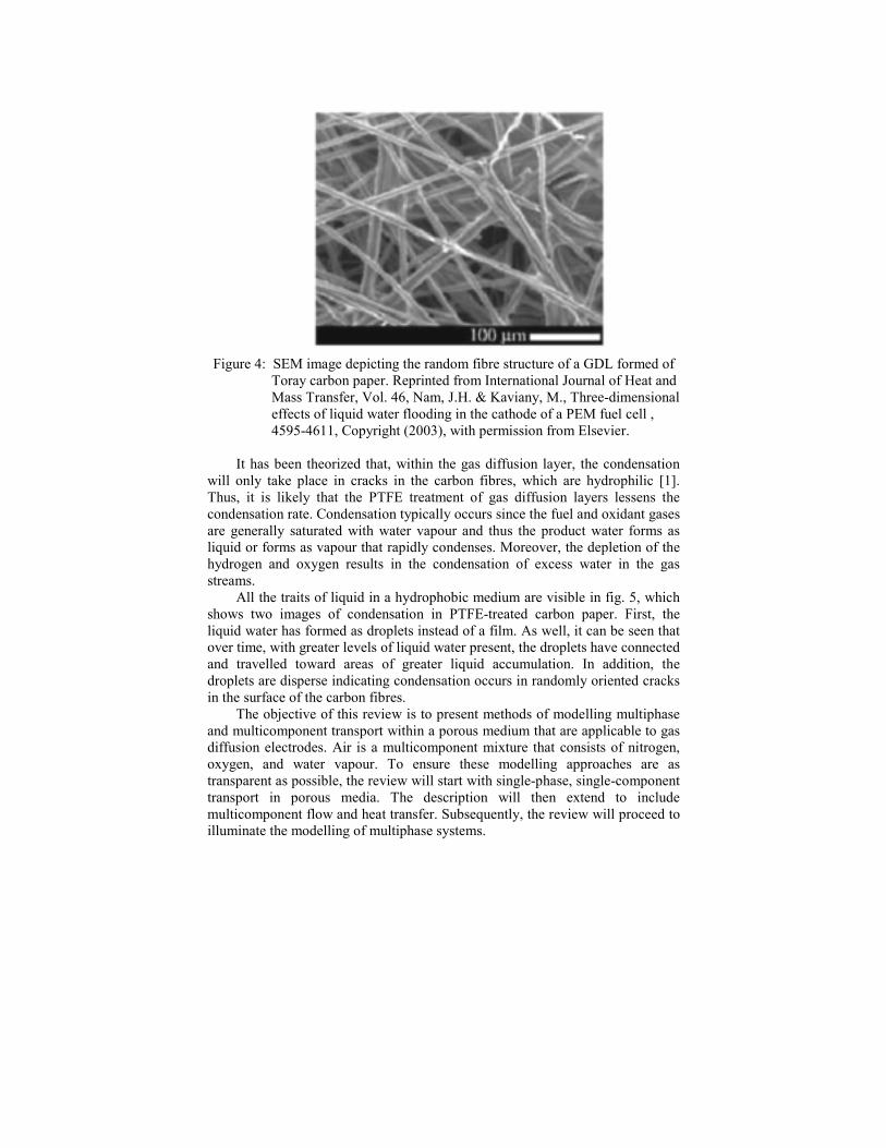
Figure 4: SEM image depicting the random fibre structure of a GDL formed of

Toray carbon paper. Reprinted from International Journal of Heat and Mass Transfer, Vol. 46, Nam, J.H. & Kaviany, M., Three-dimensional effects of liquid water flooding in the cathode of a PEM fuel cell , 4595-4611, Copyright (2003), with permission from Elsevier.

It has been theorized that, within the gas diffusion layer, the condensation

will only take place in cracks in the carbon fibres, which are hydrophilic [1]. Thus, it is likely that the PTFE treatment of gas diffusion layers lessens the condensation rate. Condensation typically occurs since the fuel and oxidant gases are generally saturated with water vapour and thus the product water forms as liquid or forms as vapour that rapidly condenses. Moreover, the depletion of the hydrogen and oxygen results in the condensation of excess water in the gas streams.

All the traits of liquid in a hydrophobic medium are visible in fig. 5, which shows two images of condensation in PTFE-treated carbon paper. First, the liquid water has formed as droplets instead of a film. As well, it can be seen that over time, with greater levels of liquid water present, the droplets have connected and travelled toward areas of greater liquid accumulation. In addition, the droplets are disperse indicating condensation occurs in randomly oriented cracks in the surface of the carbon fibres.

The objective of this review is to present methods of modelling multiphase and multicomponent transport within a porous medium that are applicable to gas diffusion electrodes. Air is a multicomponent mixture that consists of nitrogen, oxygen, and water vapour. To ensure these modelling approaches are as transparent as possible, the review will start with single-phase, single-component transport in porous media. The description will then extend to include multicomponent flow and heat transfer. Subsequently, the review will proceed to illuminate the modelling of multiphase systems.

Figure 5: Environmental scanning electron micrography (ESEM) image

depicting condensatin on Toray carbon paper. a) At time = t. b) At time = t + ∆t. Reprinted from International Journal of Heat

and Mass Transfer, Vol. 46, Nam, J.H. & Kaviany, M., Three-dimensional effects of liquid water flooding in the cathode of a PEM fuel cell , 4595-4611, Copyright (2003), with permission from Elsevier.

2 Single-Phase Transport

2.1 Transport of a Single-Phase with a Single Component

In the case of a single-phase with a single component in a porous medium under isothermal conditions, there are two equations required to describe the bulk hydrodynamic behaviour. These equations are the conservation of mass and the conservation of momentum. The conservation of mass in porous media is expressed as:

0)()( =⋅∇+∂

∂ ut

ρερ ( 1 )

In this case, u is the superficial velocity that takes into account the facial

porosity and is related to the average interstitial velocity (the average velocity in the pores) by:

εiuu = ( 2 )

In an isothermal system, the transport of a single fluid/species in porous

media is driven by the pressure gradient P∇ . It is universally accepted when modelling porous media as a continuum to use the generalized Darcy's equation form of the momentum conservation equation:

Pku ∇−=µ

( 3 )

where k is the permeability and µ/k is the viscous resistance.

2.1.1 Permeability The permeability of a porous medium represents its ability to conduct fluid flow through its open volume. Permeability can be obtained by applying the conservation of mass and momentum to a pore-scale model. Since most porous media feature complex geometry and are anisotropic, solutions of the permeability have only been obtained for idealized conditions. The fibrous media found in the gas diffusion layer of PEMFC electrodes is very complex and three-dimensional. Two forms of pore-scale modelling are capillary models and drag models. In capillary models, the Navier-Stokes equation is applied for ducts in serial, parallel, and networks. Drag models for approximating permeability are an application of the Navier-Stokes equation to flow over objects. CFD is now being employed at a pore level to determine permeability [2, 3]. However, if pore sizes are small enough that molecular effects require consideration (the flow inside the pore can no longer be considered a continuum), the CFD approach is inaccurate. Instead, computationally intensive methods, such as lattice-Boltzmann models, can be employed.

Another approach for evaluating permeability is the semi-heuristic hydraulic radius method, commonly referred to as the Carman-Kozeny theory. The relationship for the permeability is obtained by applying the equation for Hagen-Poiseuille flow to a pore with an approximated hydraulic diameter. The derivation results in the following equation:

2

32

)1(36 εε−

=k

por

kd

k ( 4 )

where pord is the characteristic pore diameter and kk is Kozeny constant. The Kozeny constant is evaluated from a shape factor (2 for circular capillaries) multiplied by the tortuosity factor (roughly 2.5 for a packed bed). Thus, the permeability of a packed bed is often obtained by using a Kozeny constant of 5. An alternative to analytical/semi-analytical methods is to rely on empirical data to determine for the permeability value. An outline for determining permeability experimentally is given by Biloé and Mauran [4].

2.2 Transport of a Single-Phase with Two Components

The presentation of single-phase multicomponent transport will begin with the equation for the conservation of a single species in a binary mixture. If there are more than two species that can be considered dilute, their diffusion can be approximated as binary diffusion with the species of the greatest concentration (the background species). With the addition of new species and variation in

concentration, the viscosity and density of the mixture change. These changes can be accounted for in a variety of manners. The simplest method is volume averaging. However, Bird et al. [5] offers more theoretical approximations for the mixture viscosity. These values should then be used in the momentum conservation equation (see eqn. (3)). With the exception of the dependence of the viscosity and density on the concentrations of the species, the hydrodynamic equations are unchanged.

Herein, mass fluxes ( An ), mass concentration ( Aρ ), and mass fractions ( Ay ) will be used to describe velocities and distributions in multicomponent systems. These variables can be transformed to their molar counterparts by each species' molar mass. The mass fraction of A is related to the concentration by

ρρ /AAy = , and the mass flux of A is related to the velocity ( Au ) of A by

AAA un ρ= . The species conservation equation in porous media for binary or dilute

multicomponent mixtures is presented in vector form as:

AAA Sn

t=⋅∇+

∂∂ )()(ερ ( 5 )

where AS is the volumetric source/sink of A . The mass flux of A ( An ) is evaluated as the mass-average flux of A ( uAρ ) plus the relative mass flux of A ( Aj ). It should be remembered that u is the superficial velocity expressed in

eqn. (2). The relative mass flux of A ( Aj ) is the Fickian diffusion term and is a

function of the effective diffusivity of A in the second species B ( effABD ) and

the gradient in the concentration of A ( Aρ∇ ).

AeffABA Dj ρ∇−= ( 6 )

Subsequently, the mass flux of A ( An ) can be evaluated with the

expression:

AeffABAA Dun ρρ ∇−= ( 7 )

By substituting the mass flux of A in eqns. (7) and (5), the mass transport equation for species A is revealed.

AAeffABA

A SDut

+∇⋅∇=⋅∇+∂

∂ )()()( ρρερ ( 8 )

Driving forces Fluxes

Velocity gradients

Temperature gradient

Concentration and pressure gradients

External force differences

Momentum

Newton’s law (viscosity)

Energy

Fourier’s law (thermal

conductivity)

Dufour effect (thermal diffusion

coefficient) Mass

Soret effect

(thermal diffusion coefficient)

Fick’s law (diffusivity)

Figure 6: Schematic of driving forces of momentum, energy, and mass transfer.

The transport coefficient associated with each phenomenon is listed. Reproduced from [5].

However, this is a simplification if the system under consideration is not

isothermal. In addition to a mass flux, the gradient in the concentration of A also drives a flux of energy. This is the Dufour effect. A mass flux of A can also be attributed to a temperature gradient. This is the Soret effect. The present review will not investigate these two additional effects, as they are generally negligible in fuel cell applications. A matrix of fluxes and their driving forces are shown in fig. 6.

2.2.1 Effective Diffusivity in Porous Media In order to account for the geometric constraints of porous media, the open space diffusivity is often corrected with geometric factors. The Bruggemann correction used by Berning and Djilali [6], and many others modelling gas diffusion layers in PEMFCs, modifies the diffusivity for porous regions with a function of the porosity:

DDeff 5.1ε= ( 9 )

However, in many pieces of literature and fundamental studies [4, 7, 8], a function of both the porosity and the tortuosity factor is adopted. The tortuosity factor is the square of the tortuosity. The tortuosity is the actual path length over the point-to-point path length as shown in fig. 7. The tortuosity factor often varies between 2 and 6, and values as high as 10 have been reported [7]. The effective diffusivity is obtained with the following relationship:

Figure 7: Schematic of tortuosity.

2

LengthPath Point Point toLengthPath Actual

=

=

τ

τε DDeff

( 10 )

The τε / term is sometimes referred to as the formation factor. The

porosity ε is a result of the area available for mass transport. The square of the tortuosity is present because of the extended path length and reduced concentration gradient that are both represented by the tortuosity. The derivation of this result is presented by Epstein [8].

The Bruggemann correction and the second expression are %5± equivalent in the region of 5.04.0 << ε with tortuosity equal to a low value of 1.5. Under all other ranges there is a significant difference between the correlations. It should be noted that the Bruggemann correction, which is widely employed and quoted, was obtained from a study on the electrical conductivity of dispersions [9]. The exponent of 1.5 was an empirically determined factor found for a specific case in the De La Rue and Tobias paper [9]. Electrical conductivity measurements are presently one of the only methods of determining the tortuosity. Measurements of the electrical conductivity are taken when a non-conductive porous media is saturated with a conductive fluid. However, this method cannot be applied to gas diffusion layers, which are electrically conductive. Nevertheless, the formation factor is determined by the ratio of the effective conductivity ek for a porous medium saturated with a fluid of known conductivity fk .

f

e

kk=

τε ( 11 )

In order to use the Bruggemann correction, it is more appropriate to replace

the exponent of 1.5 with the Bruggemann factor α . The Bruggemann factor can then be presented as a function of the porosity and the tortuosity factor.

)(log)/(log

10

10

ετεα

τεε α

=

= ( 12 )

In a typical case where the porosity is equal to 0.5 and the tortuosity factor

is 3, the value of the Bruggemann factor α is 2.585. This indicates that commonly employed exponent of 1.5 may not be applicable to gas diffusion layers. Finally, a good rule of thumb for the effective diffusivity in typical porous media is a reduction of an order of magnitude.

2.2.2 Determination of the Binary Diffusion Coefficient Binary diffusivities ABD are typically calculated based on an empirically developed formulation presented by Cussler [7]. This is an effective method for determining the diffusivity in a numerical model, and agrees well with published empirical data. The empirical method was implemented by Berning and Djilali [6] and is expressed in Cussler [7] as:

)(/1/1

3/13/1

75.1

BA

BAAB

MMP

TDφφ +

+= ( 13 )

where φ is the diffusion volume and M is the molar mass. Other expressions, such as the Chapman-Enskog theory [7], require the use of tabulated temperature dependant values that complicate the procedure for determining the binary diffusivity. With the knowledge of the diffusivity at given pressure oP and temperature oT , the above expression can be further simplified to:

75.1

),(

=

o

oooABAB T

TPPPTDD ( 14 )

2.2.3 Transport of a Single-Phase with more than Two Components If considering a system with n components ( 2>n ) that are not dilute, the evaluation of the diffusion becomes much more complex. With n components,

the diffusive flux of each species depends on the concentration gradient of the other 1−n species. This dependence is evident in the Maxwell-Stefan equations for multicomponent diffusion, which are expressed as:

effij

jiijn

ijji D

NxNxc

−=∇ ∑

≠= ,1

( 15 )

In the above equation, integer subscripts i and j have replaced the letter

subscripts A and B as we are no longer considering a binary system. Above, ic is the molar concentration, jix , is the mole fraction, and jiN , is the molar

flux. However, this is a difficult expression to include in a finite volume CFD code. Berning [10] suggests the use of an equivalent approach that is termed the generalized Fick's law.

2.3 Knudsen Diffusion

With diffusion in porous media, it is acknowledged that the diffusion mechanism varies with the length scale of the porous media. The Knudsen number is the non-dimensional parameter commonly employed to characterize the flow and diffusion regimes in micro-channels. The Knudsen number is the ratio of mean free path to pore diameter. When the mean free path is large in comparison to the pore diameter, the probability of molecule-molecule interaction is small and molecule-wall collisions dominate. The expression for the Knudsen number is [7]:

PdTk

dKn

iipor

B

por

22πσ

λ

=

=

( 16 )

where λ is the mean free path, pord is the pore diameter, Bk is the

Boltzmann constant, iiσ is the collision diameter, and P is the pressure. Flow in porous media can be categorized into three regimes by the Knudsen number [11]:

1. Continuum Regime, 01.0<Kn

2. Knudsen Regime, 1>Kn

3. Knudsen Transition Regime, 101.0 << Kn

In most of the literature [11, 12], the Knudsen regime is defined by 1>Kn .

However, Karniadakis [13] states the transition region corresponds to 101.0 << Kn , and the Knudsen regime to 10>Kn . In addition, Karniadakis

notes that at 1>Kn the concept of macroscopic property distribution breaks down. It is also evident in various plots in chapter 5 of in Karniadakis [13] that there is a significant difference in the flow behaviour for 11.0 << Kn , and much less variation in the flow characteristics in the region 101 << Kn . Thus, if the flow is in the upper region of the transition regime, the flow is still dominated by Knudsen diffusion according to Karniadakis. It is therefore reasonable to assume that a strictly Knudsen regime is present when 1>Kn .

In the Knudsen Regime, molecule-wall collisions dominate over molecule-molecule collisions. Similar to molecular diffusion, flux in the Knudsen regime is influenced by the gradient of the concentration of a species. The gradient of the partial pressure is the driving force. The partial pressure gradient is equal to that of the concentration for constant pressure conditions. However, a new diffusivity is defined (Knudsen Diffusivity KnD ). Knudsen diffusivity is corrected in the same manner as the molecular diffusivity in porous media. Since viscous and ordinary diffusion is negligible in the Knudsen Regime [11, 12], eqn. (7) reduces to:

AeffKn

AA

D

jn

ρ∇−=

= ( 17 )

and the mass transport equation (see eqn. (8)) is:

AAeffKn

A SDt

+∇⋅∇=∂

∂ )( ρερ ( 18 )

2.4 Determination of Knudsen Diffusivity

The Knudsen diffusion coefficient is determined from the kinetic theory of gases and is expressed as [4, 7, 14, 15]:

ApAKn M

RTdDπ8

31

, = ( 19 )

It can be inferred from the previous equation that the Knudsen diffusivity is

independent of the other species present in a system. This is because of negligible collisions between molecules. One species cannot ``learn'' about the presence of other species [12]. It follows that no additional considerations are necessary for systems with more than two components. Quoting from Cunningham [12], “In the Knudsen regime, there are as many individual fluxes present as there are species (as in molecular diffusion), and these fluxes are independent of each other (in contrast to molecular diffusion).”

2.5 Knudsen Transition Regime

The transition regime is present when 101.0 << Kn . In this regime, both molecular diffusion and Knudsen diffusion (slip flow) are present. A common way to evaluate this regime is the Dusty Gas Model (DGM) [11, 12, 14, 16, 17]. The DGM is derived by considering the solid matrix as large stationary spheres suspended in the gas mixture as one of the species present. The formulation is rigorously explained by Cunningham [12] and employed for modelling solid oxide fuel cells by Suwanwarangkul [17]. Often, the effective DGM diffusivity ( DGD ) is approximated in the case of equal molar masses [12, 18]. In these cases, the effective DGM diffusivity is calculated by:

ABAKn

ABAKnDG DD

DDD

+=

,

, ( 20 )

This diffusivity can subsequently be corrected for porous media with eqn.

(10) and then replace the binary diffusion coefficient in the mass transport equation (eqn. (8)).

2.5.1 Comparison of the Diffusivities The three diffusivities that have been presented (binary molecular diffusivity

ABD , Knudsen diffusivity AKnD , , and an effective diffusivity retrieved from the

dusty-gas model with equimolar diffusion DGD ) are now compared of a range of Knudsen numbers. This is done to depict the applicability of each diffusivity to the three diffusion regimes. The Knudsen number has been varied from 0.01 (continuum regime) to 10 (Knudsen regime). The diffusivity presented is that of oxygen in nitrogen at a temperature of 350K and a pressure of one atmosphere. fig. 8 depicts the three diffusivities.

Figure 8: Comparison of the binary molecular diffusivity DAB, Knudsen

diffusivity DKn,A, and an effective diffusivity retrieved from the dusty-gas model with equimolar diffusion DDG over a range of Knudsen numbers. Oxygen in nitrogen for a temperature of 350K and a pressure of 1atm.

fig. 8 illustrates the significant difference in approximations of the

diffusivities depending on the regime. Scanning electron micrography of Toray carbon paper [1] show voids with widths between roughly 1 and 100 µ m, corresponding to Knudsen numbers between 0.1 and 0.001. A Knudsen number of 0.1 in fig. 8 is on the boundary of the region where Knudsen diffusion is shown to dominate. This indicates that Knudsen diffusion could be of concern, but is not significant for the carbon paper shown by Nam and Kaviany [1]. Nevertheless, the smaller pore diameters (~1µm) in the catalyst layer require the consideration of Knudsen diffusion.

3 Two-Phase Systems

A large variety of applications exist for models encompassing multiphase flow, heat transfer, and multicomponent mass transfer in porous media. These include thermally enhanced oil recovery, subsurface contamination and remedy, capillary-assisted thermal technologies, drying processes, thermal insulation materials, trickle bed reactors, nuclear reactor safety analysis, high-level radioactive waste repositories, and geothermal energy exploitation [19]. As well,

this combination of transport phenomena is present when modelling the flooding of PEM fuel cell electrodes.

The phase distribution is potentially the result of viscous, capillary, and gravitational forces. The additional phase can be formed by phase change or is introduced externally into the system. Each phase can also be a multicomponent mixture and the components of each phase can in some cases be transported across phase boundaries. When modelling the diffusion layer of a PEMFC it is generally accepted that the second phase, liquid water, is comprised of single component and there is only transfer of water across the phase boundary.

For porous media in which the void space is occupied by two-phases, the bulk porosity ε is divided between the liquid lε and gas gε volume fractions.

The liquid saturation ls is the volume occupied by the liquid lε divided by the open pore volume ε . This relationship is depicted in fig. 9 and eqn. (20).

εε=

ε=ε+ε

=ε+ε+ε

ll

gl

gls

s

1 ( 21 )

3.1 Two-Phase Regimes

Two-phase flow exists in three possible regimes; pendular, funicular, and saturated. The regime present at any time and location depends on the saturation. To some degree it also depends on the wettability. The aforementioned regimes are illustrated in fig. 10. The pendular regime is predominant for low saturations where the liquid phase is discontinuous. The term “pendular” stems from the pendular rings that form around sand grains in this regime. The funicular regime occurs when the liquid is continuous and travels through the pores in a funicular (corkscrew) manner. When the saturation approaches unity, the liquid saturated regime emerges and the pores are fully occupied by the liquid.

Figure 9: Schematic of the volume fractions.

a) b) c)

Figure 10: Schematics of two-phase regimes in porous media. a) Pendular b)

Funicular c) Saturated. The saturation level at the transition between the funicular and pendular

regimes corresponds roughly to what is termed the immobile saturation (also referred to as the irreducible saturation). This saturation level is found when no more water can be removed from a two-phase test sample in a permeation test, often featuring a centrifuge. The final weight of the sample is compared to the dry weight and the immobile saturation ims is determined. This immobility is the result of surface tension. From herein, the saturation s is the reduced saturation, which is the actual liquid saturation ls scaled as follows [20]:

im

iml

ssss

−−=

1 ( 22 )

The immobile saturation can be expected to be quite high for PEM fuel cell

electrodes. This stems from the results presented by App and Mohanty [21], who showed the dependence of ims on the capillary number Ca :

σµuCa = ( 23 )

where u and µ are the velocity and viscosity of the invading phase and σ is the interfacial tension. The capillary number is the ratio of viscous forces to interfacial tension forces. High capillary numbers arise from a viscous force much greater than the surface tension forces. This could be the result of a high-velocity. One condition in which a small capillary number applies is the case of negligible velocity in either phase.

Figure 11: Schematic of two processes responsible for surpassing the immobile saturation: Increasing the capillary number through higher velocities and increasing the saturation of the liquid.

The capillary number is small in PEMFC electrodes because mass transport is dominated by diffusion and the velocity term u is quite small. App and Mohanty stated that in porous cores the immobile saturation for their low capillary number cases was 18.0=ims , whereas for large capillary numbers the immobile saturation approached zero. In addition, Kaviany [22] stated that the immobile saturation increases as the pore size is reduced.

The dependence of the immobile saturation on the capillary number can be explained by the deformation of droplets under the viscous stress of a high velocity invading phase. The viscous forces elongate the droplets that eventually bridge and form a continuous phase. At this moment the phase regime of the displaced phase transforms from a pendular regime to a funicular regime and capillary flow is initiated. fig. 11 illustrates how an increased capillary number, due to greater velocities, allows the saturation to surpass the immobile saturation. In addition, the same figure depicts how increasing liquid saturation causes the transformation from a pendular regime to a funicular regime (where the liquid is capable of motion) when the saturation surpasses the immobile saturation.

3.2 Hydrodynamics and Capillarity in Two-Phase Systems

The relationships developed for the hydrodynamics of a single-phase in porous media will now be applied to each phase in the two-phase system (gas and liquid). The conservation equations for the gas and liquid phases are:

lllll

ggggl

Sut

s

Sut

s

�

�

=⋅∇+∂

∂

=⋅∇+∂

−∂

)(

)()1(

ρερ

ρερ

( 24 )

where ε)1( ls− and εls in the first terms in the equations represents the volume

of each phase. Respectively, gS� and lS� are the volumetric sources of gas and liquid. These sources, or sinks, can arise from phase change, in which case

lg SS �� −= , or from an external source. The single-phase momentum equation, eqn. (3), is adapted to the two-phase

system in a similar fashion. The only notable difference between the single and two-phase cases is that the permeability is phase specific for the gas ( gk ) and liquid ( lk ). These permeabilities are a correction of the bulk permeability ( k ) for the effect of the reduced area open to each phase due to the presence of the other phase.

ll

ll

gg

gg

Pku

Pk

u

∇−=

∇−=

µ

µ ( 25 )

It is evident that the system is not fully defined with the general

conservation of mass and momentum equations. The four equations above cannot evaluate the five variables ( ls , gu , lu , gP , and lP ) that must be solved. This is because a prominent phenomenon in multiphase flow in porous media has not been introduced into the equation set. Expressions for the capillary pressure are employed as the constitutive relationship that completes the system of equations.

Capillarity and capillary pressure are the result of interfacial tension, which is the surface free energy between two immiscible phases. The microscopic capillary pressure is directly proportional to the interfacial tension and inversely proportional to the radius curvature of the interface. Thus, the lesser the radius of curvature, the more dominant the effects of capillary pressure. This is the microscopic definition of the capillary pressure, which is typically formulated as:

rPc

σ∝ ( 26 )

where r is the characteristic radius of the liquid/gas interface. The macroscopic definition of the capillary pressure cP , the pressure difference between the wetting gas and non-wetting liquid pressures, is included in the two-phase momentum equations (eqn. (25)). This is shown in hydrostatic form in fig. 12.

Figure 12: Hydrostatic representation of capillary pressure when the liquid is the non-wetting phase.

glc PPP −= ( 27 )

Fig. 13 is an attempt to use the microscopic and macroscopic definitions of

the capillary pressure to explain capillary motion in a pore. At the end of the pore where the liquid radius is smaller (lower local saturation), the capillary pressure is greater than at the end with the larger liquid radius (greater local saturation). Because the liquid pressure is the sum of the capillary pressure and the gas pressure, the hydrodynamic pressure of the liquid is greater at the end of the pore with the smaller radius. Therefore, the bulk motion of the liquid is toward the end with the greater radius (and local saturation).

At this point in the discussion, the transport of the liquid water in the electrodes of PEMFCs should be revisited. The transport of liquid water from low to high saturation, as shown in fig. 13, is counter-intuitive and could lead to incorrect conclusions. In a broad sense, the transport depicted in fig. 13 illustrates the penchant for water, in hydrophobic media, to move to ever-increasing pore diameters according to the capillary pressure’s inverse proportionality to the liquid radius. Ultimately, the largest radius can be attained when the liquid reaches the gas channel.

Conversely, the water invades smaller pores in the catalyst layer due to the hydrophilic nature of the electrolyte. However, the electrolyte phase in the catalyst layer offers a second mode of water transport. Water can be transported through the catalyst layer’s electrolyte in a similar fashion to that of the electrolyte membrane. Though, a review of these transport issues is beyond the scope of the present chapter and shall be reserved for a separate discussion of transport phenomena in polymer electrolyte membranes.

Figure 13: Schematic of capillary diffusion, in which the liquid is the non-wetting phase.

Subsequent to the definition of the macroscopic capillary pressure, the

momentum equations take the form:

cl

lg

l

ll

gg

gg

PkPku

Pk

u

∇−∇−=

∇−=

µµ

µ ( 28 )

When interfacial tension is observed as driving mass transport due to a

gradient in the capillary pressure, the phenomena is referred to as capillary diffusion. The mass flux of the liquid phase due to capillary diffusion can be obtained from the second term of the liquid momentum equation (eqn. 28):

cl

lsl Pkm ∇−=

µρ

,� ( 29 )

If the gradient of the capillary pressure is assumed to rely only on the

saturation gradient, the liquid transport due to capillary diffusion emerges as:

ll

c

l

lsl s

dsdPkm ∇

−=

µρ

,� ( 30 )

and thus the capillary diffusivity is often defined [19]:

=

l

c

l

ll ds

dPksDµ

)( ( 31 )

Now the momentum equations for the two-phase system (eqn. (28)) can be

reformulated to eliminate the liquid pressure field from the equation set. Inserting the definition of capillary diffusivity into the liquid momentum equation yields a function of the gas pressure and the liquid saturation.

llgl

ll ssDPku ∇−∇−= )(

µ ( 32 )

It is important to note that the interfacial tension, which capillary diffusion

is a result of, is not constant in a non-isothermal and multicomponent system [19]:

),( AcTσσ = ( 33 )

Therefore, diffusion due to interfacial forces can be driven by temperature

and concentration gradients in addition to saturation. These two transport mechanisms are termed thermal- and solutal-capillary diffusion:

AA

c

l

lcl

c

l

lTl

cc

Pkm

TT

Pkm

A∇

∂∂

∂∂=

∇

∂∂

∂∂=

σσµ

ρ

σσµ

ρ

,

,

�

�

( 34 )

As with capillary diffusion, the thermal- and solutal-capillary diffusivities

can be derived. However, these terms are often not included because of their negligible contributions to the total mass flux.

Figure 14 Contact angle for hydrophobic and hydrophilic fluid/solid interfaces.

Another characteristic of two-phase flow in porous media, which needs to

be introduced before proceeding, is the surface tension between the liquid phase and solid matrix. The surface tension is dependant on the wettability, or the hydrophobicity, of the liquid/solid interface. Fig. 14 depicts the effect of hydrophobicity on the contact angle θ . Hydrophobic interfaces feature a contact angle greater than 90 � . Teflon (PTFE) features a contact angle of 108 � . For hydrophobic solids, the gas is the wetting phase. Hydrophilic interfaces feature a contact angle less than 90 � . In this case, the liquid is the wetting phase. The contact angle θ can be calculated from the gas-liquid σ , gas-solid gsσ , and

liquid-solid lsσ interfacial tensions:

σσσ

θ lsgs −=)cos( ( 35 )

There have been corrections developed for the contact angle in porous

media as an alternatively to using the contact angle on a flat plate. It has been found that the effective contact angle porous media is less than the actual [23]. This indicates that the porous form of a material is less hydrophobic than the bulk form. An important note on surface tension is that it is known that transport of liquid water increases with the contact angle (more hydrophobic). This trend could be due to the reduced contact area between the porous media and the liquid (see fig. 14), which increases the influence of the viscous forces exerted by the invading phase. This increased liquid transport is a reason for the impregnation of electrode diffusion layer with PTFE.

3.2.1 Capillary Pressure Curves In order to use the capillary pressure as a constitutive relationship, an expression for the capillary pressure is derived. It would be too difficult to determine the capillary pressure microscopically as in fig. 13. Thus, a volume averaging approximation is utilized. The starting point for derivation this constitutive relationship is the form of capillary pressure curves obtained in experiment. In these experiments, the capillary pressure is measured in a sample and compared to the estimated level of saturation [23]. The form of curves generated is shown in fig. 15.

Figure 15: General form of the capillary pressure curve. It was postulated by Leverett [24] that the capillary pressure versus

saturation relationship could be presented in the non-dimensional form:

2/1

)(

=εσkPsJ c ( 36 )

This function is typically referred to as the Leverett J-function. Occasionally, a cosine of the contact angle θ is included in the Leverett J-function [1]:

2/1

)cos()(

=εθσkPsJ c ( 37 )

However, Anderson [23] stated that this is not valid for modelling the effects of wettability on capillary pressure.

Udell [20] later used data presented by Leverett [24] to determine the J-function for the porous media in Leverett’s experiments. Udell then compared experimental results with a one-dimensional steady-state model for packed sand. The porosity was varied from 0.33-0.39 and permeabilities from

12103.1039.1 −×− m 2 . Good agreement between the model and the experiment was presented. The J-function Udell obtained is often referred to as the Udell function, which is expressed as:

32 )1(263.1)1(120.2)1(417.1)( ssssJ −+−−−= ( 38 )

There are also many other J-functions [22], including Scheidegger's [25]:

08.0005.0)1(221.0)1(364.0)( )1(40

−+−+−= −−

ll

s

ssesJ l ( 39 )

The above J-function (eqn. (39)) is then employed to calculate the capillary

pressure with the formula:

)()/(

)cos(2/1 sJ

kPc ε

θσ= ( 40 )

As well, van Genuchten [26] presented a relation for the capillary pressure,

which is a function of saturation and requires empirical constants:

( )nm

sPnm

c

/11

11 /1

−=

−=α ( 41 )

Kaviany [22] stated that the capillary pressure curves must be bounded by

the relationship:

−∞=→ ds

dPcss iml

lim ( 42 )

Observing the dsdPc / derivative in eqn. (30), it could be inferred that

Kaviany's boundary (eqn. (42)) would predict a very large mass flux at iml ss ≈ . However, this is also the point at which the liquid is in transition between the pendular and funicular regimes. Thus, the high capillary pressure is due to the immobility of the discontinuous phase. Therefore, the mass flux is limited.

Fig. 16 presents these various capillary pressure relationships as a function of saturation. Experimental results presented by Anderson [23] are also plotted. It is evident that the experimental results abide by Kaviany's boundary, whereas the capillary pressure expressions do not. Another flaw of these expressions is that the result is the same whether imbibition (increasing ls ) or drainage (decreasing ls ) is being considered (when it has been clearly shown that there is a significant difference in reality [22, 23].

Figure 16: Capillary pressure curves from various relations and experimental results. For Udell and Scheidegger’s: k ≈ 10-11 m2, ε = 0.35, and σ = 0.0644 N/m (air/water). For Anderson’s plot: air and water in an interfacial Teflon core. For van Genuchten’s: n = 2 and α ≈ 7 x 10-21.

Many other expressions for the capillary pressure exist. However, they are

not presented herein. As with Leverett and Udell's work, these relations are for packed sand and other representations of soil. There is a significant lack of material evaluating capillary pressure in fibrous porous media.

3.3 Relative Permeability

When two or more phases occupy the same pores, the amount of pore space available for each phase is reduced. Referring to eqn. (4) it is acknowledged, at least theoretically, that the permeability is a function of the porosity. Therefore, the permeability must be adjusted for the volume fractions occupied by different phases. The permeabilities of the gas and the liquid are now expressed as:

Figure 17: General form of the relative permeability functions.

kkk

kkk

rll

rgg

=

= ( 43 )

where k is the single-phase permeability. Fig. 17 depicts the general form of relative permeability functions used for the gas and liquid phases. In addition, the immobile saturation for the phases is mathematically accounted for in the relative permeability. The relative permeabilities are commonly expressed as:

3)1( skrg −= ( 44 ) 3skrl = ( 45 )

where s is the reduced saturation (see eqn. (22)). Some explanation for the cubic form of these equations can be found in the Carman-Kozeny equation (see eqn. (4)), where the single-phase permeability is roughly proportional to

23 )1/( εε − .

Figure 18: Relative Permeability of displaced phase (gas) for various degrees of hydrophobicity. θ = 108o corresponds to nitrogen displaced by liquid water in an artificial Teflon core (Anderson, 1987, b).

Figure 19: Relative Permeability of displacing phase (liquid) for various degrees of hydrophobicity. θ= 108o corresponds to nitrogen displaced by liquid water in an artificial Teflon core (Anderson, 1987, b)

Recalling that the more dominant the interfacial tension the higher

immobile saturation, it is evident that interfacial tension and the wettability/hydrophobicity has an effect on the relative permeability. The effect of wettability on the relative permeabilities was surveyed by Anderson [27]. Fig. 18 presents the relative permeability of gases for a large range of contact angles. The case of �108=θ is that of nitrogen displacing water in a Teflonized core. This is a good approximation of the PEMFC electrode. Equation (44) is plotted to evaluate its validity. Firstly, it is evident that the gas permeability presented by Anderson is apparently bimodal for all degrees of wettability. However, the often prescribed cubic function is monotonic. It is also evident in fig. 18 that eqn. (44) would underestimate the relative permeability at low saturations and would predict values significantly higher than the experimental results show in the high saturation regions.

Fig. 19 depicts the effect of wettability on the displacing phase (water) permeability as presented by Anderson [27]. The plots indicate that the immobile saturation resides between 0.16 and 0.20. The plot also depicts a uniform effect of wettability on the relative permeability. It is clear in the plot that a hydrophobic porous structure aids the transport of water by increasing the permeability of the structure. Again, the cubic relative permeability function (eqn. (45)) is plotted for comparison. It can be seen that the cubic function follows the liquid curves to a higher degree than the gas curves. It is evident that eqn. (45) approximately predicts the relative permeability for interfaces featuring a contact angle of �100 , which is slightly hydrophobic.

It is noted that the relative permeability is seen to increase rapidly at higher saturations, allowing effective water transport. However, the gas phase is shown in fig. 18 to reach its immobile saturation at a liquid saturation of 0.6 for the hydrophobic cases. At this point, the permeability of the gas reduces to zero.

Figure 20: Classification of PEMFC electrode models.

4 Multiphase Flow Models

With a clear understanding of the transport phenomena in porous media with non-isothermal multiphase flows, the models prescribed in literature can be evaluated for use in PEM fuel cell electrodes. Fig. 20 classifies the models by their features. The distinguishing features include the accounting of liquid water, convection of the liquid water by the gas, transport of liquid water due to surface tension effects (capillary diffusion), or whether the liquid is considered to be stationary. The characterization of the various multiphase models that can be applied to the gas diffusion layer in a PEM will start with most generalized case (multi-fluid) and work toward the most specific version (porosity correction).

4.1 Multi-Fluid Model

The multi-fluid model presented herein is the application of the equations developed previously to a porous medium occupied by air and liquid water. The air is treated as a multicomponent mixture and the liquid phase is considered as immiscible water. In the multi-fluid model, as employed for fuel cells by Berning and Djilali [6], each phase is modelled with its own set of field equations. The two-phases are coupled by the relative permeabilities, which are sensitive to saturation, and phase change terms.

The steady state conservation equations:

( )( ) cmu

cmu

pll

pgg

�

�

−=⋅∇

=⋅∇

ρρ

( 46 )

The momentum equations:

ssDPku

Pk

u

lgl

ll

gg

gg

∇−∇−=

∇−=

)(µ

µ ( 47 )

The species conservation equation in Berning and Djilali [6] was applied

only to the gas phase and is the single-phase species conservation equation (eqn. (8)) with modification of the liquid saturation to account for the reduced volume fraction open to the gas. The steady state conservation of species A in the gas phase can be presented as:

( ) AA

effAAg SDu �+∇⋅∇=⋅∇ ρρ )( ( 48 )

where eff

AD is the diffusivity of species A and AS� is the phase change source term, which is zero except in the water vapour conservation equation.

4.1.1 Rate of Phase Change To complete the multi-fluid model, an expression for the rate of phase change between the gas and liquid phases must be introduced. The phase change between the gas and liquid can be either evaporation or condensation, depending on the local properties. However, the knowledge of molecular dynamics during phase change is still considered limited [28]. A starting point for the exploration of phase change is the kinetic theory of gases. The main principle when modelling phase change with kinetic theory is that there is a maximum amount of vapour that can be accommodated at vapour/liquid interface. This maximum accommodation is the mass transfer limiting characteristic. Thus, through the application of the kinetic theory of gases, the maximum rate of evaporation for a liquid can be determined.

The goal of recent research in kinetic phase change is the approximation of evaporation and condensation coefficients. The coefficients are ratios of actual mass transfer to the theoretical maximum rate. Eames et al. [28] and Marek and Straub [29] offer reviews of previously obtained values for a variety of circumstances.

The kinetic theory approximation allows for the consideration of thermal equilibrium, or differences in the temperature between the gas and liquid phases. The expression for the rate of mass transfer per unit area of gas/liquid interface

( OHm2

� ), when the gas and liquid are in thermal equilibrium, was presented by Eames et al. [28] as:

))((2

2/12

2 vsOH

kOH PTPR

Mm −

=

πγ� ( 49 )

where )(TPs is the water vapour saturation pressure and vP is the partial pressure of the water vapour in bulk gas stream. kγ is the kinetic evaporation coefficient, which is equivalent to the condensation coefficient under thermal equilibrium conditions. The magnitude of evaporation coefficients measured in experiments can range from 0.001 to 1 [29].

A second approach assumes the liquid phase exists in the form of a spherical droplet. In such a case, the mass transfer is determined from the diffusion rate between the bulk gas and the surface of the droplet. In addition, a mass transfer Nusselt number is employed as a dimensionless measure of a droplet's ability to exchange mass. In its present form, this method applies only to systems featuring local thermal equilibrium. The Nusselt number for mass transfer ( mNu ) from a liquid droplet to the surrounding gas is [5]:

3/12/16.00.2 ScReNum += ( 50 )

where Sc is the Schmidt number ( )/(

2OgHgg Dρµ ) and Re is the Reynolds

number ( greldg uD µρ / ). dD is the droplet diameter and relu is the relative velocity between the gas and the droplet. The droplet's mass transfer coefficient ( dγ ) can be obtained by multiplying the Nusselt number by the diffusivity of water vapour in the gas ( vgD ) and the inverse of the droplet diameter ( dD/1 ).

dmvgd DNuD /=γ ( 51 ) The mass transfer coefficient is subsequently multiplied by the difference

between the density of water vapour in water-saturated air ( sρ ) and the density of water vapour in the bulk gas ( vρ ) to approximate the mass transfer per unit area of gas/liquid interface. See fig. 21 for clarification of these two densities.

Figure 21: Schematic of droplet evaporation for thermal equilibrium.

)(2 vsdOHm ρργ −=� ( 52)

This method of determining mass transfer rate was implemented in the

modelling of a PEM fuel cell by Berning and Djilali [6, 10]. A simplification required to use this model was to use a mean droplet diameter rather than the actual. Another appropriate assumption is that since the velocities in the gas diffusion layer are small enough, the Nusselt number reduces to 2.0 [5]. Therefore, eqn. (52) can be expressed as:

)(2

2 vsd

vgOH D

Dm ρρ −=� ( 53)

Berning and Djilali [6] also included a correction factor (ω ) for reduced

phase change rates in porous media:

)(2

2 vsd

vgOH D

Dm ρρ

ω−=� ( 54)

When implementing either of the two aforementioned methods of

calculating the rate of phase change, the total interfacial area between the gas and liquid ( glA ) phase must be determined to calculate the total mass transfer

( OHM2

� ). This is typically achieved with the area of a spherical droplet of a mean

diameter ( 2dDπ ). The number of droplets ( dn ) in a representative volume (V ) is

the volume of liquid ( Vslε ) divided by the volume of a single droplet ( 361

dDπ ).

36

d

ld D

Vsnπε= ( 55)

Thus, the interfacial area is:

d

lgl D

VsA ε6= ( 56)

and the total mass transfer in volume V is:

OHglOH mAM22

�� = ( 57)

4.1.2 Application The multi-fluid model is the most general and, conceptually, the most flexible as it relies on less restrictive assumptions. An example of the application of this model to fuel cells is shown in Figs. 22-24 [10].

Fig. 22 shows iso-contours of oxygen and water vapour concentrations. In these plots, as in subsequent figures, the top and bottom of the vertical axis correspond to the catalyst layer/ GDL and channel/GDL interfaces, respectively, and the planes correspond to successive locations from the inlet to the outlet of the fuel cell section. The molar oxygen concentration contours are similar to those found with a single-phase version of the model, with more pronounced oxygen depletion under the land areas of the collector plate. However, because of phase change, the concentration of water is relatively uniform. The 0.8% difference can be attributed to the temperature field’s influence on the saturation pressure of water.

The left-hand side of fig. 23 presents the phase change in the cathode’s GDL. Positive values correspond to evaporation, which can be found under the land areas due to the increased pressure drop. The pressure drop, an artifact of the increased resistance to gas transport below the land area, reduces the vapour pressure below the saturation point. Negative values, indicating condensation, are most prevalent at the catalyst layer/GDL interface because of the oxygen consumption and the production of water vapour.

On the right-hand side of fig. 23 the distribution of liquid water saturation in the cathode’s GDL is shown. For this current density (0.8 A/cm2) , a maximum saturation of 10% is obtained under the land area at the end of the channel. The gradient of the saturation is from high levels at the catalyst layer to low levels at the channel interface. This reflects the implementation of the well-posed hydrophilic formulation of the capillary transport, in which water travels from high to low saturation.

The velocity vectors of the gas and liquid phases are presented in fig. 24. The gas phase, shown on the left, indicates the bulk transport of gas to the catalyst layer. In a single-phase model, the bulk motion of the gas is in the opposite direction due to the removal of product water vapour. However, when

phase change and capillary transport are accounted for, the removal of product water is, in the most part, by the liquid phase. This is evident in the plots of the liquid phase velocity vectors on the right-hand side of fig. 24.

Figure 22: Molar oxygen concentration (left) and water vapour distribution (right) inside the cathodic gas diffusion layer at a current density of 0.8A/cm2 [10].

Figure 23: Rate of phase change [kg / (m3 s)] (left) and liquid water

saturation [-] (right) inside the cathodic gas diffusion layer at a current density of 0.8A/cm2 [10].

Figure 24: Velocity vectors of the gas phase (left) and the

liquid phase (right) inside the cathodic gas diffusion layer at a current density of 0.8A/cm2 [10].

The broader applicability of the multi-fluid model comes at the cost of

solving for an additional set of field equations and the required coupling of the phases. This makes the numerical solution much more challenging and computationally intensive. In particular, the convergence rates and the numerical stability of the model can be problematic under some operating conditions. Alternative models based on various levels of simplifications are presented below. Though they are less general, these models can be more practical and can be effective in simulating transport in the GDL, provided they are used for appropriate regimes.

4.2 Mixture Model

The mixture model has been used to model two-phase flow in PEM electrodes by several researchers, including Wang et al. [30] and You and Liu [31]. The main theme of the mixture model is the description water transport, as vapour and liquid, with traditional mixture theory practices. The resulting equation set is mathematically equivalent to the multi-fluid model [19]. The reformulation is obtained by utilizing phase quantities that are relative to that of the mixture. The set equations employed in the mixture model for steady state conditions are as follows.

The mixture conservation equation is:

0)( =⋅∇ uρ ( 58) The mixture momentum equation is:

PKu ∇−=ρν

( 59)

where ν is kinetic viscosity of the mixture. The mixture species conservation equation is expressed as:

[ ]

⋅∇−

∇−∇⋅∇

+∇⋅−∇=⋅∇

∑∑==

kkA

lgkA

kA

kAkk

lgk

AAA

jyyyDs

yDuy

,,

)(

...)()(

ρε

ερργ

( 60)

where the advection correction factors Aγ in eqn. (60) account for the specific velocity fields encountered by each species. The advection correction factor is formulated as:

( )

gAgg

lAll

gAg

lAl

A ysysyy

ρρλλρ

γ+

+= ( 61)

where the kλ terms are the relative mobilities for the gas and liquid phases. They are expressed as:

lrlgrg

lrll

lrlgrg

grgg

kkk

kkk

νννλ

ννν

λ

///

///

+=

+=

( 62)

The mixture quantities are evaluated as:

)/()/(1

grglrl

ggglll

gAgg

lAllA

gAgg

lAllA

ggll

ggll

kk

hshsh

DsDsD

ysysy

uuu

ss

ννν

ρρρρρρ

ρρρ

ρρρρρρ

+=

+=

+=

+=

+=

+=

( 63)

The individual phase velocities are extracted from the solution in the post

processing stage. These velocities are found with the addition of relative velocities to the mixture velocity ( lg

lglglg juu ,,,, += ρλρ ). Accounting only for

capillary diffusion, the relative mass flux term kj in eqn. (60) is expressed as:

lg

ll

cgll

jj

sdsdPkj

−=

∇

=

νλλ

( 64)

The liquid saturation is calculated and updated with each iteration. It is

determined by comparing the total water concentration with the concentration of water vapour required to saturate the gas phase. If the concentration of water is greater than saturation concentration, then liquid water must be present. Using the expression for the total density of water ( OH 2

ρ ) as a function of liquid water

saturation ( ls ), and the saturated gas and liquid concentration of water ( sρ and

lρ respectively),

vlllOH ss ρρρ )1(2

−+= ( 65)

the saturation can be determined. It is important to note that sρ is the mass of water vapour per unit volume of water vapour saturated air (the mass fraction of the water vapour in the air multiplied by the bulk density of water vapour). sρ can be extracted from the temperature dependent saturation pressure of air ( )(TPs ), the absolute gas pressure ( P ), and the bulk density of water vapour ( vρ ):

vs

s PTP ρρ )(= ( 66)

Considering a pure liquid phase, eqn. (65) can be rearranged as:

sl

sOHls

ρρρρ

−−

= 2 ( 67)

Thus, the saturation can be calculated from the total water concentration, temperature, and pressure.

4.3 Moisture Diffusion Model

The moisture diffusion model, also referred to as unsaturated flow theory [19], was developed to determine the transport of liquid water when the only driving force is capillarity. Luikov [32] and Whitaker [33] are considered pioneers of this formulation. This method was applied to PEM fuel cells by Natarajan and Nguyen [34]. The steady state transport equation for liquid water in the moisture diffusion model can be expressed as (Wang and Cheng, 1997):

( ) 0)( =+∇⋅∇ lll SssD � ( 68) where

l

c

l

lll s

pksD∂∂=

µρ)( ( 69)

OHgl SS2,

�� −= ( 70)

and S� is the mass source due to phase change. The moisture diffusion model could be incorporated into a CFD code by treating the liquid phase as a scalar species with no convection terms. This would be a moderately easy method of incorporating two-phase flow into a single-phase fuel cell model. The mass sources need to be calculated in the form of a rate as in the multi-fluid model. In addition, the porosity would require a correction based on the liquid saturation.

4.4 Porosity Correction Model

The porosity correction model simplifies the present two-phase problem by neglecting the transport of liquid water. The saturation level is computed with each iteration. In the Kermani et al. [35] model, the temperature and the level of saturation are calculated iteratively by the internal energy and density of the water in the system.

Subsequently, the volume fraction open to the gas phase is reformulated as:

)1( sg −= εε ( 71) This model is particularly efficient when saturation levels are low (below

the immobile saturation limit for the liquid water). This model would be the simplest to append to an existing single-phase fuel cell model.

4.5 Evaluation of the Multiphase Models in the Literature

Table 2 is provided to help determine which model should be employed given the conditions of the system, the porous media considered, and the computational resources available. At one extreme is the multi-fluid model. The multi-fluid model is a strong candidate when an abundance of computational resources is available and stable phase coupling can be achieved. At the other extreme is the porosity correction model. This model is an ideal candidate, due to its computational efficiency when considering saturation levels below the immobile value.

Table 2: Advantages, disadvantages, and areas of application for each of the multiphase flow models.

Multiphase Flow Model

Advantages Disadvantages Areas of Application

Multi-fluid Model

- Generalized form. - Interphase transfer models can be used. - Can resolve complex liquid motion. - Models convection of liquid by the gas. - Can model species diffusion in liquid.

- Highest number of variables. - Needs the most computational resources. - Coupling of the phases can lead to unstable models. - Requires a multiphase CFD code.

- Best employed for high saturation conditions because of the need for greater liquid resolution. - When the influence of the gas on the liquid is equivalent to that of the surface tension.

Mixture Model

- Reduced number of variables. - Models the influence of the gas pressure on the liquid.

- May have trouble converging at higher saturations (liquid and gas have significantly different velocity fields). - Cannot employ interphase transfer models. - Large number of mixture quantities to calculate.

- Best used when the gas pressure is the dominant force on the liquid or when capillary forces drive the liquid in the same direction. - High capillary number (i.e. large pores and high permeability).

Moisture Diffusion Model

- One additional equation over one-phase model. - Can employ phase change models.

- Does not account for the influence of the gas pressure on the liquid. - Cannot model interphase transfer of heat and species.

- When surface tension is the dominant force on the liquid. - Low capillary numbers (i.e. small pores and low permeability).

Porosity Correction Model

- No additional transport equations over the one-phase model.

- Does not account for liquid motion.

- Conditions where the liquid saturation does not exceed the immobile saturation (i.e. low relative humidities, very small pores, and low current densities).

5 Outstanding Issues and Conclusions

A number of fundamental issues need to be addressed in order to devise reliable predictive tools for two-phase transport in gas diffusion electrodes. These include: � The hydrodynamic and diffusive properties of the porous media in the

electrodes need to be characterized. The structure of PEM fuel cell gas diffusion layers is typically fibrous. In the case of carbon cloth layers, the porous matrix is constructed from woven tows of fibres producing macro- and micro-pores. Alternatively, carbon paper layers are a formation of randomly laced fibres. It is obvious that the architecture of

gas diffusion layers is significantly different to that of packed beds, or cylindrical pores in a monolithic structure that are often the object of porous media studies. It is also clear that these fibrous layers are anisotropic. Some parameters to be resolved are the three-dimensional tensors for the area porosity, permeability, and tortuosity. At present, the properties can only be implemented in an isotropic form in the available commercial CFD codes.

• The capillarity in the electrode's porous media requires significant research. Current expressions used to determine capillary pressure in electrodes are based on studies of packed beds and rarely include the influence of wettability. Issues to be resolved include the presentation of a capillary pressure versus saturation curve for a gas diffusion layer, the immobile saturation levels for gas and liquid, and the influence of wettability on those properties.

In closing this discussion, we note that mass transport limitations continue

to be a significant hindrance to achieving higher current densities in PEM fuel cells. Water management within these fuel cells is a key consideration in their design. Knowledge of the behaviour of liquid water in electrodes is limited by the inability to make in situ measurements. Better understanding of the transport of water in the PEMFC electrode can be obtained from models that capture the important physical processes. Several specific models of two-phase mass transport have been outlined and discussed in this Chapter. These models, once implemented in a CFD code, will be able to help fuel cell designers improve their understanding of the transport of liquid water, as well as the transport of reactant and product gases, in the porous electrodes. It is clear from this review that a critical area to advance modelling of two-phase transport in gas diffusion electrode is further experimental characterization of the porous materials employed in PEM fuel cells.

References

[1] Nam, J.H. & Kaviany, M., Effective Diffusivity and Water-Saturation Distribution in Single- and Two layer PEMFC Diffusion Medium. Int. J. Heat Mass Transfer, 46:4595-4611, 2003.

[2] Ngo, N.D., & Tamma, K.K., Microscale permeability predictions of porous fibrous media. Int. J. Heat Mass Transfer, 44:3135-3145, 2001.

[3] Papathanasiou, T.D., Flow across structured fiber bundles: a dimensionless correlation. J. Multiphase Flow, 27:1451-1461, 2001.

[4] Biloé, S. & Mauran, S., Gas flow through highly prous graphite matrices. Carbon, 41:525-537, 2003.

[5] Bird, R.B., Stewart, W.E. & Lightfoot, E.N., Transport Phenomena. John Wiley and Sons, New York, 1960.

[6] Berning, T. & Djilali, N., A Three-Dimensional, Multi-Phase, Multicomponent Model of the Cathode and Anode of a PEM Fuel Cell. J. Electrochem. Soc. 150: A1598-A1607, 2003.

[7] Cussler, E.L., DIFFUSION-Mass Transfer in Fluid Systems. Cambridge University Press, New York, 1997.

[8] Epstein, N., On tortuosity and the tortuosity factor in flow and diffusion through porous media. Chem. Eng. Sci., 44(3):777-779, 1989.

[9] De La Rue, R.E. & Tobias, C.W., On the Conductivity of Dispersions. Journal of Electrochemical Society 106(9), 1959.

[10] Berning, T., Three-Dimensional Computational Analysis of Transport Phenomena in a PEM Fuel Cell. PhD thesis, University of Victoria, 2002.

[11] Kast, W. & Hohenthanner, C.R., Mass transfer within the gas-phase of porous media. Int. J. Heat Mass Transfer, 43(5):807-823, 2000.

[12] Cunningham, R.R. & Williams, R.J.J., Diffusion in gases and porous media. Plenum Press, New York, 1980.

[13] Karniadakis, G.E. & Beskok, A., Micro Flows-Fundamentals and Simulation. Springer- Verlag, New York, 2002.

[14] Feng, C. & Stewart, W.E., Practical Models for Isothermal Diffusion and Flow of Gases in Porous Solids. Ind. Eng. Chem. Fundam., 12(2), 1973.

[15] Taylor, R., Calculation of Steady-State Multicompnent Mass Transfer Rates in Porous Media in the Transition Region. Ind. Eng. Chem. Fundam., 21:63-67, 1982.

[16] Staia, M.H., Cambell, F.R. & Hills, A.W.D., Measurement of Gaseous Diffusion Coefficents in Porous Reaction Products. Ind. Eng. Chem. Res., 26:438-446, 1987.

[17] Suwanwarangkul, R., Croiset, E., Fowler, M.W., Douglas, P.L., Entchev, E. & Douglas, M.A., Performance comparison of Fick's, dusty-gas and Stefan-Maxwell models to predict the concentration overpotential of a SOFC anode. J. Power Sources, 122:9-18, 2003.

[18] Mezedur, M.M., Kaviany, M., & Moore, W., Effect of Pore Structure, Randomness and size on Effective Mass Diffusivity. AIChE Journal, 48(1):15-24, 2002.

[19] Wang, C.Y. & Cheng, P., Multiphase Flow and Heat Transfer in Porous Media. Advances in Heat Transfer, 30:30-196, 1997.

[20] Udell, K.S., Heat transfer in porous media considering phase change and capillarity-the heat pipe effect. Int. J. Heat Mass Transfer, 28(2):485-495, 1985.

[21] App, J.F. & Mohanty, K.K., Gas and condensate relative permeability at near-critical conditions: capillary and Reynolds number dependence. J. Petrol. Sci. Eng., 36:111-126, 2002.

[22] Kaviany, M., Principles of Heat Transfer in Porous Media. Springer-Verlag, New York, 1991.

[23] Anderson, W.G., Wettability literature survey - Part 4: Effects of wettability on capillary pressure, J. Petrol. Technol., 1283-1299, Oct. 1987.

[24] Leverett, M.C., Capillary behaviour in porous solids. AIME Trans., 142:152-169, 1941.

[25] Scheidegger, A.E., The physics of flow through porous media. University of Toronto Press, Toronto, 1974.

[26] van Genuchten, M. Th., A closed-form equation for predicting the hydraulic conductivity of unsaturated soils. Soil Sci. Soc. Amer. J., 44:892-898, 1980.

[27] Anderson, W.G., Wettability literature survey - Part 5: Effects of wettability on relative permeability. J. Petrol. Technol., pages 1453-1468, Nov. 1987.

[28] Eames, I.W., Marr, N.J. & Sabir, H., The evaporation coefficient of water: a review. Int. J. Heat Mass Transfer, 40(1):2963-2973, 1997.

[29] Marek, R. & Straub, J., Analysis of the evaporation coefficient and the condensation coefficent of water. Int. J. Heat Mass Transfer, 44:39-53, 2001.

[30] Wang, Z.H., Wang, C.Y. & Chen, K.S., Two-phase flow and transport in the air cathode of proton exchange membrane fuel cells. J. Power Sources, 94:40-50, 2001.

[31] You, L., & Liu, H., A two-phase and transport model for the cathode of PEM fuel cells. Int. J. Heat Mass Transfer, 45:2277-2287, 2002.

[32] Luikov, A.V., Systems of differential equations of heat and mass transfer in capillary-porous bodies (Review). Int. J. Heat Mass Transfer, 18:1-14, 1975.

[33] Whitaker, S., Simultaneous heat, mass and momentum transfer in porous media: A theory of drying. Advances in Heat Transfer, 13:119-203, 1977.

[34] Natarajan, D. & Nguyen, T.V., Three-dimensional effects of liquid water flooding in the cathode of a PEM fuel cell. J. Power Sources, 115:66-80, 2003.

[35] Kermani, M.J., Stockie, J.M., & Gerber, A.G., Condensation in the Cathode of a PEM Fuel Cell. Proc. of the 11th Annual Conference of the CFD Society of Canada, 2003.

SAMPLE SYMBOLS AD Droplet area Agl Area of gas-liquid interface c Molar concentration Ca Capillary number dpor Pore diameter D Diffusion coefficient DAB Diffusion coefficient in a binary system Dij Diffusion coefficient in a multicomponent system D(sl) Capillary diffusion coefficient Dd Droplet diameter j Relative mass flux k Permeability kg,l Relative permeability kB Boltzmann constant kk Kozeny constant Kn Knudsen number

OHm 2� Phase change mass transfer M Molecular weight n Mass flux N Molar flux Num Mass transfer Nusselt number P Pressure Pc Capillary pressure Ps Saturation pressure R Universal gas constant s Reduced saturation sim Immobile saturation sg,l Phase saturation S Mass source term Sc Schmidt number t Time T Temperature x Mole fraction y Mass fraction u Superficial velocity ui Average interstitial velocity V Volume VD Volume of droplet Greek Letters γ Mass transfer coefficient γA Advection correction factor ε Porosity λ Mean free path λg,l Relative mobility

µ Viscosity ν Kinematic viscosity ρA Density of species A ρ Density σ Interfacial tension σii Collision diameter τ Tortuosity factor φ Diffusion volume ω Phase change correction factor