two new approaches to depth-of-field post-processing...
TRANSCRIPT

Two New Approaches to Depth-of-Field Post-Processing:Pyramid Spreading and Tensor Filtering
Todd J. Kosloff1 and Brian A. Barsky2
1 Computer Science Division, University of California, Berkeley, CA [email protected]
2 Computer Science Division and School of Optometry,University of California, Berkeley, CA 94720
Abstract. Depth of field refers to the swath that is imaged in sharp focus throughan optics system, such as a camera lens. Control over depth of field is an im-portant artistic tool, which can be used, for example, to emphasize the subjectof a photograph. The most efficient algorithms for simulating depth of field arepost-processing methods. Post-processing can be made more efficient by mak-ing various approximations. We start with the assumption that the point spreadfunction (PSF) is Gaussian. This assumption introduces structure into the prob-lem which we exploit to achieve speed. Two methods will be presented. In ourfirst approach, which we call pyramid spreading, PSFs are spread into a pyramid.By writing larger PSFs to coarser levels of the pyramid, the performance remainsconstant, independent of the size of the PSFs. After spreading all the PSFs, thepyramid is then collapsed to yield the final blurred image. Our second approach,called the tensor method, exploits the fact that blurring is a linear operator. Theoperator is treated as a large tensor which is compressed by finding structure init. The compressed representation is then used to directly blur the image. Bothmethods present new perspectives on the problem of efficiently blurring an im-age.
1 Introduction
In the real world it is rare for images to be entirely in perfect focus. Photographs, films,and even the images formed on our retinas all have limited depth of field, where someparts of the image are in-focus, and other parts appear blurred. The term “depth of field”technically refers to the portion of the image that is in focus. In the computer graphicsliterature, the term “depth of field” is used to refer to the effect of having some objectsin focus and others blurred. Computer generated images typically lack depth of fieldeffects. Simulating depth of field requires significant computational resources.
Computer generated images are typically rendered based on a pinhole camera model.A pinhole camera model assumes that all light entering the camera must pass through asingle point, or pinhole. Pinhole cameras allow only a very small amount of light to en-ter the camera, thus they are of limited utility for real world cameras. Pinhole camerasare efficient to simulate because they are geometrically the simplest type of camera.However, these models lead to images where all objects are in perfect focus.
To allow more light to enter the camera an aperture of some size, instead of a pin-hole, is used. A lens is needed to avoid the scene being highly blurred. However, a lenshas to be focused at a single depth. The light from objects located at any other distancefrom the lens does not converge to a single point, but instead forms a disk on the cam-era’s sensor or film. Since sensors and film have a finite resolution, as long as the diskis smaller than a film grain or pixel of a sensor, the object will appear in perfect focus.However, blur occurs when the disk is large enough to be resolved.
2 Background
Depth of field simulation was first introduced to the computer graphics community byPotmesil and Chakravarty [13]. They used a post-processing approach based on bruteforce; thus, their method was quite slow. A great deal of work has since been done onfinding faster methods of depth of field post-processing. Bertalmio and Sanchez-Crespo[3] used a heat diffusion method to blur efficiently. Kass [8] also used a heat diffusionapproach for depth of field post-processing. Zhou [18] used a separable approxima-tion to the blur operation in order to increase speed. Scheuermann [14] used a sparseapproximation to the blur, coupled with working at a reduced resolution for the mostblurred regions. Scofield [15] introduced the simple yet useful idea that depth of fieldcan be simulated by treating the scene as a set of layers, each of which can be blurredefficiently using an FFT convolution. Kosloff [10] introduced an efficient depth of fieldmethod based on fast rectangle spreading.
Post-processing methods cannot always achieve the highest quality, but there areslower approaches available that produce very high quality results. One approach toincreasing quality is to improve the fidelity of the post-processing approach at the costof performance, e.g. Shinya’s ray distribution buffer [16]. Another approach is to accu-rately simulate geometric optics, thus generating very high quality results. Such meth-ods include Cook’s distributed ray tracing [4], Dippe’s stochastic ray tracing [6] andHaeberli and Akeley’s accumulation buffer [7].
Readers interested in learning more about previous depth of field algorithms shouldconsult the following surveys: [1, 2, 5]
3 Spreading and Gathering
3.1 Spreading
Spreading is a type of filter implemented as follows: for each input pixel determine thePSF and place it in the output image, centered at the location of the input pixel. ThePSFs are summed to determine the output picture.
Spreading filters are appropriate for depth of field and motion blur, due to the imageformation process. In the case of depth of field, each pixel in the input image can beroughly thought of as corresponding to a point in the input scene. Each point in theinput image emits or reflects light, and that light spreads out in all directions. Some ofthat light enters the lens and is focused towards the film. This light forms the shape of acone. If the point is in perfect focus, the apex of the cone will hit the image plane (film,
retina, sensor, etc). When the apex of the cone hits the image plane, the scene point isimaged in perfect focus. When a different part of the cone hits the sensor, the point willimage as a disk of some kind, i.e. a PSF. The image formation process suggests thatspreading is the correct way to model depth of field. The pyramid spreading filter wasmotivated by the need for depth of field post-processing.
A bright point of light ought to image as a PSF with size and shape determined bythat point. In a post-processing method, it is easy to simply spread each input pixel andget the desired effect. For a gather filter to handle PSFs correctly, it would have to con-sider that potentially any pixel in the input image could contribute to any output pixel,each with a different PSF. The effective filter kernel for this high quality gather methodwould have a complicated shape that would depend on the scene. This complicatedshape prevents acceleration methods from being effective.
3.2 Gathering
Gathering is a type of filter that is implemented as follows: the color of each output pixelis determined by taking a linear combination of input pixels, typically from the regionsurrounding the location of the desired output pixel. The input pixels are weighted ac-cording to an application-dependent filter kernel.
Gathering is the appropriate type of filter for texture map anti-aliasing, as will beclear when we examine how anti-aliasing works. Texture map anti-aliasing works as fol-lows: when a textured object is viewed from a distance, the texture will appear relativelysmall on the screen. Several, or even many, texels will appear under each pixel in therendered image. Since the texture mapping is many to one, the appropriate thing to dois to average all the texels that fall under a pixel. The averaging should use appropriateweights; generally weights that fall off with distance. Clearly, texture map anti-aliasingis a gathering process, because each output pixel is found by averaging several inputpixels. Gathering can be used to blur images, but the results will suffer from artifacts.Our tensor method will use gathering as an internal component, but it also uses spread-ing a component. This helps to mitigate the artifacts that otherwise would be caused bygathering.
4 Overview
This paper describes two new depth of field post-processing methods that operate un-der two completely different principles. The first method, which we call the pyramidmethod is related to Potmesil and Chakavarty’s method which spreads a highly realisticPSF for each pixel. We achieve speed by making an approximation; rather than usingrealistic PSFs, we use Gaussians. Because Gaussian PSFs are band-limited, they can berepresented accurately at low resolution as long as appropriate reconstruction is laterused. This means that filtering by spreading Gaussians is more efficient, even for largeGaussians.
The second method, which we call the tensor method, is based on a tensor analysisof the blur operation, and is not particularly related to any previous method. Intuitively,we can figure that blur is a “smooth” process. Clearly, the output will be smooth because
it is blurred, but beyond this, it is important to realize that the blur operator itself issmooth. This concept of the blur operator will be explained in more detail in section5. The important consequence of a smooth blur operator is that the smoothness can beexploited to speed things up. Essentially, smooth regions are “boring”, so, relativelylittle effort needs to be expended, compared to non-smooth regions.
5 Pyramid Spreading
5.1 Algorithm
Our first fast spreading method is based on pyramids, and can be viewed as runningmipmapping in reverse. The pyramid has its final level set to the resolution of the im-age. First, the pyramid is initialized to all zeros. Next, each pixel in the input image isspread by selecting a level of the pyramid, and writing a PSF to that level (see Program1). Larger PSFs are written to coarser levels, thereby keeping the cost approximatelyconstant with respect to the PSF size. It is straightforward to outfit this method witha speed/quality tradeoff; although writing to finer levels enables more control over thePSF appearance, writing to coarser levels is faster. The final step is to upsample thecoarse levels through the pyramid, collapsing the pyramid into a final, blurred image(see Program 2). Care must be taken to use upsampling filters that are sufficiently wide,otherwise block artifacts can appear. See Figure 2 for an example of a pyramid and theresulting blurred output.
Since the number of levels that a pyramid has is finite, it is challenging to representPSF sizes that lie between two pyramid levels. We considered two possible solutionsto this difficulty. The first approach is to write to both of those two levels, each at anintensity proportional to where the continuous value truly lies. The second solutionis to write to the finer level, using a slightly larger PSF to compensate for being attoo fine a level. Both of these methods increase quality, but incur additional cost. Inpractice, the first method was found to produce superior results insofar as interpolatingbetween two smooth PSFs of different size happens to produce the appearance of anintermediate sized PSF. Although writing a slightly larger PSF to a slightly finer leveldoes indeed lead to a PSF of the correct intermediate size, this PSF will undergo avisible discontinuity if its size is increased or decreased such that it lands in a differentlevel. Even though the size is correct, PSFs at different levels appear different, due todifferent rasterizations at different levels.
It is worth delving into the details of how to properly spread PSFs to a given level,and how to upsample the pyramid. Although these operations could be implemented invarious ways, great care must be taken to produce the smoothest possible images, freeof grid artifacts.
During spreading, we want to place a PSF located at a position dictated by the lo-cation of a pixel in the input image. However, since the PSF is being spread to a coarsepyramid level, the PSF must be rendered with subpixel accuracy. Issues of how to prop-erly anti-alias the PSF can be simplified if we restrict ourselves to Gaussian PSFs, withGaussian anti-aliasing filters. A Gaussian convolved with another Gaussian is simply alarger Gaussian, and thus our filtered PSF is simply a Gaussian of slightly larger size.

Fig. 1. When computing a subpixel Gaussian, the continuous distance between Gaussian centerand pixel center is taken. It is critical that the Gaussian center is not snapped to a pixel location.
(a) Finest pyramid level. (b) Middle pyra-mid level.
(c)Coarsestpyramidlevel.
(d) Output of upsampling thispyramid.
Fig. 2. The pyramid method spreads PSFs to various pyramid levels, then upsamples the levelsthrough the pyramid to yield a final, blurred image.
The analytical nature of Gaussians makes them straightforward to render with subpixelprecision (see Figure 1). For each pixel within the support of the Gaussian, determinethe distance from the floating-point-valued center to the integer-valued pixel center.This distance provides the distance within the Gaussian, with subpixel accuracy.

During upsampling, the pixels from the coarse layer should blend together in thefiner layer such that no grid artifacts are introduced. This is done by calculating eachpixel in the finer layer as a weighted average of pixels in the coarser level. The weightedaverage is performed using a subpixel Gaussian in a manner very similar to the spread-ing step.
5.2 Performance
The cost of spreading a Gaussian depends on the resolution of Gaussian that we chooseto use. However, larger Gaussians can get written to coarser levels of the pyramid, soall Gaussians have approximately the same resolution, hence the same cost.
We found that at least 7x7 Gaussian is necessary to produce sufficiently smoothresults. The effect of intermediate sizes are achieved by writing to two different levels.This means that 7*7*2, or 98 writes, are required per pixel. This means that the pyramidmethod is an expensive method. This is necessary if we wish our PSFs to be effectivelyperfect Gaussians.
The cost of upsampling the pyramid must also be taken into account. For each levelof the pyramid except for the coarsest, upsampling from the next coarsest level mustoccur.
Since the entire pyramid can fit into a space somewhat less than twice as big as thefinest level, we bound the cost by calculating the cost of upsampling 2∗N pixels. Eachpixel that must be upsampled requires spreading 7x7 pixels, to achieve high quality.Therefore, we bound the cost of upsampling by 98∗N writes.
6 Tensor Filter
6.1 Algorithm
The second method is known as the tensor method, because it is derived from an anal-ysis of the blur tensor. To build intuition, we will develop the algorithm for the case ofapplying a 2D matrix to a 1D image vector. Then the full version of this method has asimilar derivation, but for applying a 4D tensor to a 2D image. Fortunately, it will notbe necessary to work in 4D. The full algorithm will be clear once the simplified versionhas been elucidated.
The tensor method works by exploiting structure in the matrix. We need to find away to simplify the matrix such that the matrix vector multiplication is more efficient. Asimple type of matrix is one that is separable, meaning it can be factored into the outerproduct of two vectors. Given the factorization, the matrix vector multiplication can beapplied simply by multiplying the input vector by the factors. Although blur matricesare not separable, we can still exploit this idea of separable matrices to our advantage.
The first idea was to decompose the matrix into blocks, and then approximate eachblock as being separable, but this turned out not to be an accurate approximation, thuswe tried using the singular value decomposition (SVD) to achieve a better approxima-tion. The SVD can be used to find the best low-rank approximation to a matrix, forany given rank. A matrix of rank N can be efficiently multiplied (if N is sufficiently

Fig. 3. Using the SVD to find the best separable approximation of blocks within the matrix. Fromleft right, the blocks are of increasingly small size.
small), because it is the sum of N separable matrices. We used the SVD to find thebest low-rank approximation for each of the blocks (see Figure 3). Although this SVDmethod does work, it does not lead to the same level of performance gains that ourtensor method achieves. Furthermore, the blur matrices for reasonable sized images areso large that computing the SVD would be prohibitively expensive. Finally, all theseproblems notwithstanding, the SVD would have to be taken ahead of time, offline, as apreprocess, making this method useless for dynamic scenes.
(a) A radially symmetric Gaussian can factored into two vectors. Multiplying by these two vec-tors is much more efficient than multiplying by the original matrix.
Fig. 4. A radially symmetric Gaussian can be factored into the outer product of two one dimen-sional Gaussians.

A better idea is to directly exploit the smoothness of the matrix by downsampling it.A matrix can be understood as smooth if we view it as a grayscale image, and that imageappears smooth. The larger the magnitude of the blur we are applying, the smoother thematrix is; this enables coarser samplings without losing any detail. Given the coarsematrix, we then need a way to apply that matrix to the full-resolution vector. This isdone by observing that we could reconstruct the original matrix by using reconstructionkernels. Reconstruction kernels restore the original matrix by spreading a Gaussian foreach sample. However, we do not in actuality want to reconstruct the original matrix,but merely want to calculate the effect of its multiplication. Fortunately, our Gaussianreconstruction kernels are separable (see Figure 4), so we can apply them to the vectordirectly from their factorization as the outer product of two vectors. We have effectivelyrepresented our matrix as overlapping separable matrices. The overlapping nature ofour sub-matrices is a critical difference compared to the SVD method. The massivepreprocessing of the SVD method is also avoided, since the subsampled matrix can becomputed much more easily than the SVD.
Fig. 5. A blur matrix can be adequately reconstructed by Gaussians placed down the diagonal. Forillustrative purposes, this example is for 1D blurring, i.e. we are only blurring horizontally. Left:the blur matrix constructed out of Gaussians down the diagonal. Center: Every other Gaussianremoved, to make the remaining Gaussians more visible. Right: The result of blurring an imagewith the matrix on the left.
Fortunately it is unnecessary to sample the matrix on a full 2D grid. Rather, samplescan be placed only down the diagonal (see Figure 5). This is because the blur matrixhappens to have all of its energy (nonzero values) centered around the diagonal. Theband of energy has varying size, depending on how much blur is required. To handlethis varying size, the reconstruction kernels must also have varying size. Substantialtime is saved by only sampling on the diagonal compared to sampling on a full grid.
The application of a separable Gaussian matrix has a direct interpretation in termsof spreading and gathering. First, we multiply by the row vector. Multiplication by therow vector is a gathering operation, computing a weighted average of the elementsof the input vector. The filter kernel for this gathering operation is itself a Gaussian.Second, this scalar weighted average is multiplied by the column vector to determinethe output. Since our separable matrices are overlapping, we sum them to get the blurred

image, because our tensor is constructed as the sum of separable blocks. This means thatapplication of the column vector involves summing Gaussians, a spreading operation.Therefore each separable matrix involves a gather, followed by a spread.
Given this interpretation, it is straightforward to extend the method from 1D imagesto 2D images. Simply select a number of sites (locations) in the image, and specify aGaussian size for each site. The locations and size of the sites will need to be determinedby consulting the blur map. For each site, perform a gather followed by a spread. It isclear that this works just as well in 2D as it did in 1D.
The remaining challenge is figuring out how many Gaussians to place and whereto place them. If we place too many, performance will be slow. But if we place toofew, there will be gaps in the blurred image. If we don’t place them with just the rightspacing, the blurred image will contain artifacts. To simplify, first consider how theplacement should work for the case where the blur amount is the same throughout theimage. This simplification enables constant spacing and a constant size for all the sites.We can control the amount of blur by varying the spacing between sites, close togetherfor less blur, or farther apart for more blur. The Gaussians must be large enough tocause them to overlap without leaving gaps, but the Gaussians should not be too large,however, or else performance will degrade and excessive blur will occur.
We could consider storing the results of the gathering phase, and viewing each ofthese values as a pixels in an image. Although not actually necessary, it is useful forbuilding intuition. The resulting image would be a lower resolution version of the inputimage. The Gaussians in the row vectors would be the downsampling filters. Later, ap-plying the column vectors recreates a full resolution image, effectively upsampling witha Gaussian reconstruction kernel. When viewed in this manner, the tensor filter algo-rithm is simply a new way of viewing the tried-and-true blur method of downsamplingfollowed by upsampling (see Figure 6). The blur is caused because the low resolutionimage is incapable of representing fine details.
Fig. 6. The tensor method for uniform blur is equivalent to downsampling followed by upsam-pling.

To extend this method to the general case of an arbitrarily varying blur map, we needa way to place sites with a density that varies according to the blur map. This is similar tothe importance sampling problem in rendering, which places more samples in importantareas to gather light more effectively. Our problem is also similar to stippling from non-photorealistic rendering, where points are placed to indicate variations in shading. Weconsidered borrowing a couple of methods from the importance sampling and stipplingliterature, but we eventually settled on something far simpler.
For each pixel, consider the possibility of inserting a site. We will not place a site atevery pixel, but we will rather skip a number of pixels based on the desired amount ofblur. We calculate a variable called skip level, which is simply a scaled version of theblur map value for that pixel. The scale factor was determined by trial and error. Next,the decision about whether or not to insert a site is made by modding the pixel locationwith skip level. This very simple method has the effect of placing points with exactlythe right density, in a spatially varying way. The simplicity means that the method isfast and easy to implement (see Program 3).
This very simple method of placing points has a limitation: there is no way of beingsure that any sites at all will be placed on small but very blurred objects. In fact, suchobjects can be missed completely. To really make this method useful in the general case,a more sophisticated site placement method is needed, one that can make sure that noobjects are missed. We find this method useful, not as a tool to be used in practice, butrather as a new and interesting way of thinking about the structure of the blur operator.
One solution to this problem is to use a more sophisticated method for placing thesites. A useful way to think of this problem is to consider that we are compressing theblur map. Since the sites are sparsely placed, there are relatively few degrees of freedomfor controlling the amount of blur. A useful fact from study of human perception is thatthe more blur there is, the more difficult it is to perceive differences in the amountof blur. Therefore, in regions with a lot of blur, we can get by with fewer sites. Thequadtree method exploits this structure by representing blurred regions of the blur mapwith large nodes (see Figure 7). This is the standard method for compressing an imagewith a quadtree. We then place a site at the center of each leaf node. The quadtreebuilding process ensures that no detail is lost, because sites are always placed whereneeded.
Each application of a site involves a gather followed by a spread. This means thatit is possible to accelerate the tensor filter by using fast gathering and spreading tech-niques. Any gathering method that enables Gaussian filter kernels can be used, and anyspreading method that enables Gaussian PSFs can be used. In practice Heckbert’s re-peated integration technique is the fastest choice for gathering, and the pyramid methodis the fastest choice for spreading. The reason to use the tensor filter is simplicity, since itis the easiest to implement of all the fast blur methods, and gives a high quality Gaussianblur. If fast gather and spread methods were added, this would defeat the simplicity byadding complexity. Therefore, we suggest using the tensor method in its original form,rather than in accelerated form.

(a) A blur map. (b) Sites selected via a quadtreethat compresses the blur map.
(c) Output of using the ten-sor method with sites located atthe center of the quadtree leafnodes.
Fig. 7. Illustration of the tensor method with a quadtree used to layout the sites.
6.2 Performance
It is easiest to analyze performance if we restrict to the case of uniform blur. For eachsite, there is a gather and a spread. The uniform case is easy because the size of thegathers and spreads are constant. The number of sites is inversely proportional to thesize of the blur, but the cost of each site is directly proportional to the size of the blur.Therefore, the total cost of the tensor filter is constant, since the added cost of blurringlarger Gaussians is offset by the fact that fewer Gaussians are required.
6.3 Results
We have run the pyramid method on several different images, both low dynamic range(LDR) and high dynamic range (HDR). The LDR comparisons are shown in Figures8 and 9, while Figures 10 and 11 provide the HDR comparisons. An example of thetensor method is given in Figure 12.
We have also included a couple of competing algorithms, for comparison purposes.This includes the square spreading method and the naive spreading method.
We can see that the pyramid method produces quality as high as the naive method,but in a fraction of the time. The speed of the pyramid method is not as fast as therectangle method, but quality is substantially improved.
We configured the tensor method two different ways. First, using naive gatheringand spreading, and second using the pyramid method, both in a gathering and in aspreading formulation.
7 Conclusion
We introduced two new methods for depth of field post-processing with a GaussianPSF. The first approach is based on a pyramidal formulation in which small Gaussian

PSFs are spread to images of various size. The second method treats the blur operationas a large four-dimensional tensor.
The key idea that underlies both methods is that Gaussian blur is a special operationthat possesses a great deal of structure. Direct methods, such as spatial-domain convo-lution, completely ignore the structure, thus they lead to very long render times. UsingFFT convolution is faster because it exploits the case where the PSF is the same sizethroughout an image. Our pyramid method takes advantage of the band-limited natureof Gaussians. A large Gaussian can be represented at a low resolution without any lossof detail. Of course, an upsampling step is required to smooth the low resolution imageinto the full resolution image. The tensor method exploits the fact that the blur tensorfor Gaussian blur can be represented as the sum of overlapping 4D Gaussians. Thisrepresentation is particularly advantageous because Gaussian matrices are separable,which enables them to be applied efficiently via a row and column factorization.
The pyramid method is simpler in concept than the tensor method which involvesfour dimensional tensors. Although the tensor method is complicated to explain, it isstraightforward to implement, whereas the pyramid method is difficult to implementcorrectly, despite its simplicity. The pyramid method requires that the subpixel Gaus-sians be precisely calibrated so as to prevent the occurrence of blocky artifacts. Thepyramid method is a spreading method, and the tensor method is a combination ofspreading and gathering. Therefore the pyramid method may lead to higher quality im-ages in some cases.
References
1. B. A. BARSKY, D. R. HORN, S. A. KLEIN, J. A. PANG, AND M. YUF, Camera modelsand optical systems used in computer graphics: Part i, image based techniques., in Proceed-ings of the 2003 International Conference on Computational Science and its Applications(ICCSA’03), 2003, pp. 246–255.
2. B. A. BARSKY, D. R. HORN, S. A. KLEIN, J. A. PANG, AND M. YUF, Camera modelsand optical systems used in computer graphics: Part ii, image based techniques., in Proceed-ings of the 2003 International Conference on Computational Science and its Applications(ICCSA’03), 2003, pp. 256–265.
3. M. BERTALMIO AND P. FORT AND D. SANCHEZ-CRESPO (2004) Real-time, accuratedepth of field using anisotropic diffusion and programmable graphics cards. 3DPT 04: Pro-ceedings of the 3D Data Processing, Visualization, and Transmission, 2nd International Sym-posium. 767–77, IEEE Computer Society.
4. R.L. COOK, T. PORTER AND L. CARPENTER 1984. Distributed raytracing. SIGGRAPH Comput. Graph. 18, 3 (Jul. 1984), 137-145. DOI=http://doi.acm.org/10.1145/964965.808590
5. J. DEMERS, GPU Gems, Addison Wesley, 2004, pp. 375–390.6. M. DIPPE AND E .WOLD SIGGRAPH 1985 Conference Proceedings, 1985, pp. 69–787. P. HAEBERLI AND K. AKELEY (1990) The accumulation buffer: hardware support for high-
quality rendering, In SIGGRAPH ’90: Proceedings of the 17th annual conference on Com-puter Graphics and interactive techniques, Dallas, TX, USA, pp. 309–318.
8. M. KASS, A. LEFOHN, D. OWENS (2006) Interactive depth of field using simulated diffu-sion on a GPU. Pixar Animation Studios Tech Report.
9. R. KOSARA, S. MIKSCH AND H. HAUSER (2001) Semantic depth of field. Proceedings ofthe 2001 IEEE Symposium on Information Visualization (InfoVis 2001), pp. 97-104, IEEEComputer Society Press.
10. T. KOSLOFF, M. TAO, AND B. BARSKY, Depth of field postprocessing for layered scenesusing constant-time rectangle spreading, in GI ’09: Proceedings of Graphics Interface 2009,pp. 39–46.
11. T.J. KOSLOFF AND B.A. BARSKY (2007) An algorithm for rendering generalized depthof field effects Based on Simulated Heat Diffusion, In Proceedings of the 2007 Interna-tional Conference on Computational Science and Its Applications (ICCSA 2007), KualaLumpur, 26-29 August 2007. Seventh International Workshop on Computational Geometryand Applications (CGA’07) Springer-Verlag Lecture Notes in Computer Science (LNCS),Berlin/Heidelberg, pp. 1124-1140 (Invited paper).
12. T. PORTER AND T. DUFF, Compositing digital images In SIGGRAPH Comput. Graph. 18,3 (Jul. 1984), pp. 253–259
13. M. POTMESIL AND I. CHAKRAVARTY, Synthetic image generation with a lens and aperturecamera model, in ACM Transactions on Graphics 1(2), 1982, pp. 85–108.
14. T. SCHEUERMANN AND N. TATARCHUK, Advanced depth of field rendering, in ShaderX3:Advanced Rendering with DirectX and OpenGL, 2004.
15. C. SCOFIELD, 2 1/2-d depth of field simulation for computer animation, in Graphics GemsIII, Morgan Kaufmann, 1994.
16. M. SHINYA, Post-filtering for depth of field simulation with ray distribution buffer, in Pro-ceedings of Graphics Interface ’94, Canadian Information Processing Society, 1994, pp. 59–66.
17. A. VEERARAGHAVAN, R. RASKAR, A. AGRAWAL, A. MOHAN AND J. TUMBLIN, Dap-pled photography: mask enhanced cameras for heterodyned light fields in SIGGRAPH 2007,(Jul. 2007), pp. 69.
18. T. ZHOU, J. X. CHEN, AND M. PULLEN, Accurate depth of field simulation in real time, inComputer Graphics Forum 26(1), 2007, pp. 15–23.
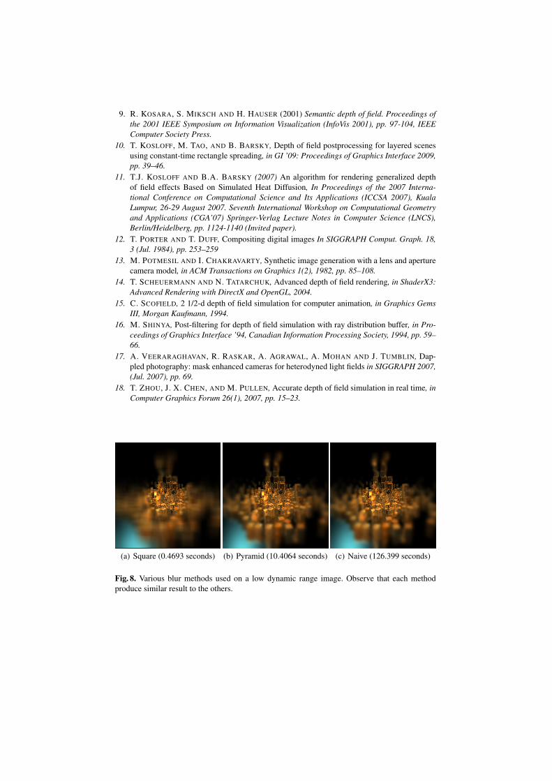
(a) Square (0.4693 seconds) (b) Pyramid (10.4064 seconds) (c) Naive (126.399 seconds)
Fig. 8. Various blur methods used on a low dynamic range image. Observe that each methodproduce similar result to the others.
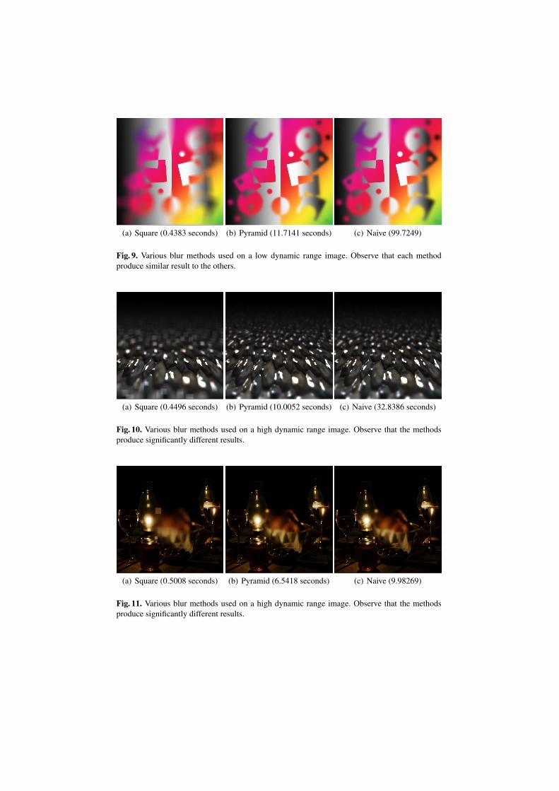
(a) Square (0.4383 seconds) (b) Pyramid (11.7141 seconds) (c) Naive (99.7249)
Fig. 9. Various blur methods used on a low dynamic range image. Observe that each methodproduce similar result to the others.
(a) Square (0.4496 seconds) (b) Pyramid (10.0052 seconds) (c) Naive (32.8386 seconds)
Fig. 10. Various blur methods used on a high dynamic range image. Observe that the methodsproduce significantly different results.
(a) Square (0.5008 seconds) (b) Pyramid (6.5418 seconds) (c) Naive (9.98269)
Fig. 11. Various blur methods used on a high dynamic range image. Observe that the methodsproduce significantly different results.

Program 1 Pseudocode implementing spreading to the pyramid.//Initialize pyramid
//pyramid[i] is a 2ˆi x 2ˆi image
//Therefore the levels have resolutions as follows.//The following entries fill the pyramid_widths table://pyramid_widths[i] = 2ˆi x 2ˆi
//X and Y are initially at the full resolution of the output image.//Scale them so that we are within the coordinate system of the current pyramid level.X = (X/width)*pyramid_widths[i];Y = (Y/width)*pyramid_widths[i];
int radius = 3;
float_type U;float_type V;
//Spread a 7x7 Gaussianfor(int u = -3; u <= 3; u++)for(int v = -3; v <= 3; v++){
//Find the floating point pixel location of where we are spreading toU = X + u;V = Y + v;
//Round U and V to the integer pixel grid, add .5 to get the pixel center,//and subtract from X and Y, the floating point center of the Gaussian//This yields du and dv are the floating point offset from the Gaussian//center to the pixel centerfloat_type du = (int)U - (X-.5);float_type dv = (int)V - (Y-.5);
//Compute the length of the offsetfloat_type dist = sqrt( du*du + dv*dv);
//The standard deviation was chosen by trial and error to be 1/3.float_type stddev = 1/3.0;
//Evaluate the Gaussianfloat_type G = exp(-(dist*dist)/(2*stddev*stddev));
//Divide through by the volume under the Gaussian, for normalization purposes.float_type weight = 1/(2.5*stddev*sqrt(2*3.14159));
//Cast the pixel location to an integer so we can write to the imageint iU, iV;iU = U;iV = V;
pixel_red(pyramid[i], iU,iV) += r*weight*G;pixel_green(pyramid[i],iU,iV) += g*weight*G;pixel_blue(pyramid[i],iU,iV) += b*weight*G;pixel_fourth(pyramid[i],iU,iV) += 1.0*weight*G;
}
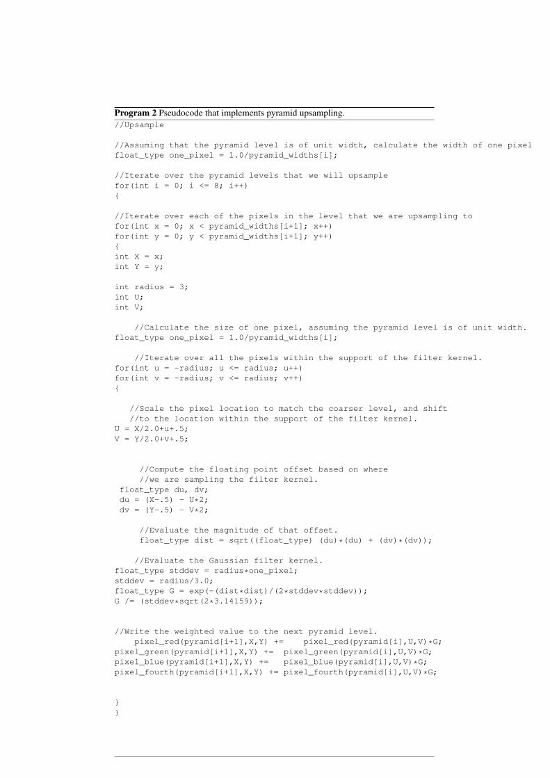
Program 2 Pseudocode that implements pyramid upsampling.//Upsample
//Assuming that the pyramid level is of unit width, calculate the width of one pixelfloat_type one_pixel = 1.0/pyramid_widths[i];
//Iterate over the pyramid levels that we will upsamplefor(int i = 0; i <= 8; i++){
//Iterate over each of the pixels in the level that we are upsampling tofor(int x = 0; x < pyramid_widths[i+1]; x++)for(int y = 0; y < pyramid_widths[i+1]; y++){int X = x;int Y = y;
int radius = 3;int U;int V;
//Calculate the size of one pixel, assuming the pyramid level is of unit width.float_type one_pixel = 1.0/pyramid_widths[i];
//Iterate over all the pixels within the support of the filter kernel.for(int u = -radius; u <= radius; u++)for(int v = -radius; v <= radius; v++){
//Scale the pixel location to match the coarser level, and shift//to the location within the support of the filter kernel.
U = X/2.0+u+.5;V = Y/2.0+v+.5;
//Compute the floating point offset based on where//we are sampling the filter kernel.
float_type du, dv;du = (X-.5) - U*2;dv = (Y-.5) - V*2;
//Evaluate the magnitude of that offset.float_type dist = sqrt((float_type) (du)*(du) + (dv)*(dv));
//Evaluate the Gaussian filter kernel.float_type stddev = radius*one_pixel;stddev = radius/3.0;float_type G = exp(-(dist*dist)/(2*stddev*stddev));G /= (stddev*sqrt(2*3.14159));
//Write the weighted value to the next pyramid level.pixel_red(pyramid[i+1],X,Y) += pixel_red(pyramid[i],U,V)*G;
pixel_green(pyramid[i+1],X,Y) += pixel_green(pyramid[i],U,V)*G;pixel_blue(pyramid[i+1],X,Y) += pixel_blue(pyramid[i],U,V)*G;pixel_fourth(pyramid[i+1],X,Y) += pixel_fourth(pyramid[i],U,V)*G;
}}
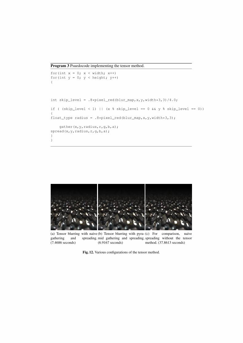
Program 3 Psuedocode implementing the tensor method.
for(int x = 0; x < width; x++)for(int y = 0; y < height; y++){
int skip_level = .8*pixel_red(blur_map,x,y,width*3,3)/4.0;
if ( (skip_level < 1) || (x % skip_level == 0 && y % skip_level == 0)){float_type radius = .8*pixel_red(blur_map,x,y,width*3,3);
gather(x,y,radius,r,g,b,a);spread(x,y,radius,r,g,b,a);}}
(a) Tensor blurring with naivegathering and spreading.(7.4686 seconds)
(b) Tensor blurring with pyra-mid gathering and spreading.(6.9167 seconds)
(c) For comparison, naivespreading without the tensormethod. (37.8613 seconds)
Fig. 12. Various configurations of the tensor method.