tutorial 5 – heads-up digitizing in arcmap · to being saved. lab 5 imagery for this tutorial,...

GEOG 245: Geographic Information Systems

Lab 05

1

Tutorial 5 – Heads-up Digitizing in ArcMap

Note: Before beginning the tutorial, copy the Lab5 archive to your server folder and unpack

it.

The objectives of this tutorial include: 1. Learning how to georegister/georeference an image

2. Creating an empty geodatabase

3. Digitizing features from an image into the geodatabase

4. Editing digitized features.

Lab Preface: Browsing on-line data

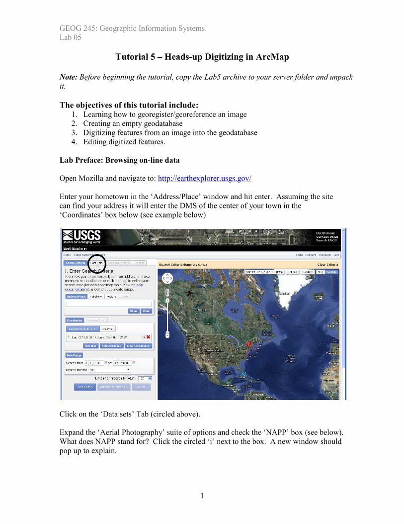
Open Mozilla and navigate to: http://earthexplorer.usgs.gov/

Enter your hometown in the ‘Address/Place’ window and hit enter. Assuming the site

can find your address it will enter the DMS of the center of your town in the

‘Coordinates’ box below (see example below)

Click on the ‘Data sets’ Tab (circled above).

Expand the ‘Aerial Photography’ suite of options and check the ‘NAPP’ box (see below).

What does NAPP stand for? Click the circled ‘i’ next to the box. A new window should

pop up to explain.


Lab 05

2

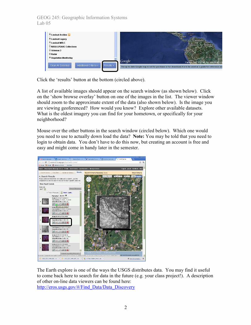
Click the ‘results’ button at the bottom (circled above).

A list of available images should appear on the search window (as shown below). Click

on the ‘show browse overlay’ button on one of the images in the list. The viewer window

should zoom to the approximate extent of the data (also shown below). Is the image you

are viewing geoferenced? How would you know? Explore other available datasets.

What is the oldest imagery you can find for your hometown, or specifically for your

neighborhood?

Mouse over the other buttons in the search window (circled below). Which one would

you need to use to actually down load the data? Note: You may be told that you need to

login to obtain data. You don’t have to do this now, but creating an account is free and

easy and might come in handy later in the semester.

The Earth explore is one of the ways the USGS distributes data. You may find it useful

to come back here to search for data in the future (e.g. your class project!). A description

of other on-line data viewers can be found here:

http://eros.usgs.gov/#/Find_Data/Data_Discovery


Lab 05

3

Heads-up Digitizing in ArcMap

Introduction

The remainder of this lab will introduce you to the creation of new GIS data using a

process called heads-up digitizing. In brief, this process involves adding a georeferenced

image in ArcMap, creating an empty geodatabase in ArcCatalog, and using ArcMap’s

drawing tools and the mouse to trace features from the image into the geodatabase. We

call this heads-up digitizing because you do this work while looking at the image on the

computer screen. The new digitized features will carry the geographic reference system

of the image.

As always, create a lab folder within your network folder and copy/unpack the Lab5 data.

Create a home/default geodatabase

Before you do anything else, you should establish your home (or default) geodatabase

into which things will be saved. This was described in an earlier lab document, but as a

reminder:

1. Launch ArcMap

2. Open the catalog window

3. Navigate to your network folder

4. Right-click on your lab 5 folder and create a New File Geodatabase.

5. Go the main ArcMap window and select Map Document Properties under the File

menu. A map document properties window will pop up.

6. Click on the little folder next to the “Default Geodatabase:” and navigate to your

new geodatabase. After hitting “Apply” this will be where your data will default

to being saved.

Lab 5 imagery

For this tutorial, you will use be using two 2008 color aerial photos to georegister a 1936

black and white air photo of the Bewkes Center.

The Bewkes Center is a Colgate-owned piece of property that has undergone significant

land cover change since the 1930's. A quick view of the 1936 image, which can be seen

below, shows large areas of open field, forest, and a lake in the middle of the property. A

copy of this image is contained in the Lab5 archive.


Lab 05

4

1936 Bewkes Photo

Unfortunately, this 1936 Bewkes image does not have any spatial reference information

(geographic and projected coordinate systems) – it is simply a digital photo. The process

of adding geographic reference information to an unreferenced image is called

georegistration (or georeferencing). This process requires that you tell ArcMap the

coordinates of at least three points on the unregistered photo. We will be using two 2008

aerial photos of the Bewkes Center as reference for the georegistration. These photos are

named c_10741024_24_19200_4bd_2008 and c_10741020_24_19200_4bd_2008. Both

are registered in the NY State Plane (central zone) coordinate system (NAD83) and the

units are feet. (Make sure you add the airphotos before you add the Bewkes image. If

you haven't, start again with a new map document. Question: Why would you do this in

this order?)

Make sure you zoom to the full extent of both layers and then add the unreferenced 1936

photo (Bewkes1936unreg.TIF) to the map document. You may not see the unregistered

map because it has no coordinate information and ArcMap does not know how to line-up

with the registered image (you will get an error like the one below telling you the layer

has no projection).

If you have not done so yet, expand the ArcMap window to the full extent of your

monitor so that you can see necessary details during georeferencing.


Lab 05

5

Georeferencing

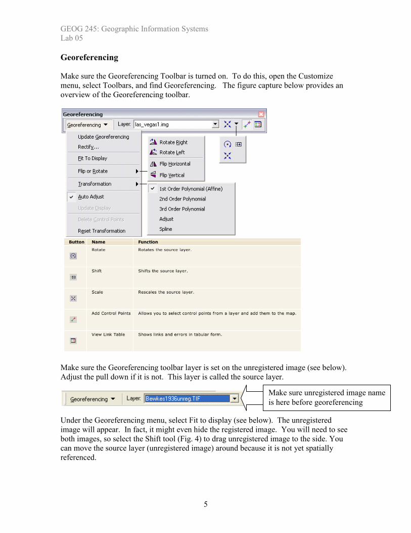
Make sure the Georeferencing Toolbar is turned on. To do this, open the Customize

menu, select Toolbars, and find Georeferencing. The figure capture below provides an

overview of the Georeferencing toolbar.

Make sure the Georeferencing toolbar layer is set on the unregistered image (see below).

Adjust the pull down if it is not. This layer is called the source layer.

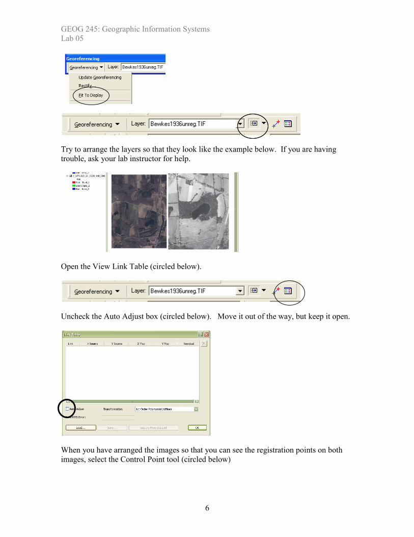
Under the Georeferencing menu, select Fit to display (see below). The unregistered

image will appear. In fact, it might even hide the registered image. You will need to see

both images, so select the Shift tool (Fig. 4) to drag unregistered image to the side. You

can move the source layer (unregistered image) around because it is not yet spatially

referenced.

Make sure unregistered image name

is here before georeferencing


Lab 05

6

Try to arrange the layers so that they look like the example below. If you are having

trouble, ask your lab instructor for help.

Open the View Link Table (circled below).

Uncheck the Auto Adjust box (circled below). Move it out of the way, but keep it open.

When you have arranged the images so that you can see the registration points on both

images, select the Control Point tool (circled below)


Lab 05

7

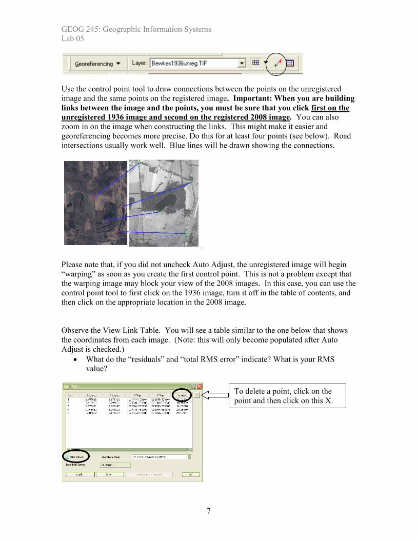
Use the control point tool to draw connections between the points on the unregistered

image and the same points on the registered image. Important: When you are building

links between the image and the points, you must be sure that you click first on the

unregistered 1936 image and second on the registered 2008 image. You can also

zoom in on the image when constructing the links. This might make it easier and

georeferencing becomes more precise. Do this for at least four points (see below). Road

intersections usually work well. Blue lines will be drawn showing the connections.

.

Please note that, if you did not uncheck Auto Adjust, the unregistered image will begin

“warping” as soon as you create the first control point. This is not a problem except that

the warping image may block your view of the 2008 images. In this case, you can use the

control point tool to first click on the 1936 image, turn it off in the table of contents, and

then click on the appropriate location in the 2008 image.

Observe the View Link Table. You will see a table similar to the one below that shows

the coordinates from each image. (Note: this will only become populated after Auto

Adjust is checked.)

• What do the “residuals” and “total RMS error” indicate? What is your RMS

value?

To delete a point, click on the

point and then click on this X.


Lab 05

8

If you make a link you don’t like, click on the link, and delete using the X on the side of

the Link Table (see arrow above). When you are done creating links, click Auto Adjust,

and you will see the 1936 image warped onto the 2008 image – (making sure the

unregistered image is lying on top of registered image).

Select the Rectify option under the Georeferencing dropdown menu. This creates an

entirely new image with the new coordinate system. Please look at the output location

– it should be pointing to your home geodatabase. What this means is that your

rectified image will be stored within your geodatabase. Give the image a new name

that indicates it is georeferenced. You can take the defaults for the other options.


Lab 05

9

Open a new map view and add your new registered Bewkes image. Make sure the image

is registered to the appropriate projection, as this image becomes the base for digitizing

the 1936 landcover.

Digitizing Bewkes Land Cover into your Home Geodatabase

In order to digitize from the registered image, you need to create a vector-format data

storage system (recall coverage, shapefile and geodatabase). In this case, we will use the

home/default geodatabase you created at the start of this tutorial. You will create

something called a “feature class” within your geodatabase and then populate it with

vector polygons that show four basic land use types: forest, non-forest, water, and

developed. You will not do it in this tutorial, but you could add more feature classes to

this geodatabase, such as a point feature class showing the locations of water fountains

and a line feature class showing roads.

Open a Catalog window, navigate to your workspace, and right click on your lab five

folder. You should see the home geodatabase you created at the start of the tutorial

(remember it looks like a small cylinder). Talk to your lab instructor if you can’t find it.

Defining an attribute domain

One of the advantages of storing your data in a geodatabase is that you can define rules

about how the data can be edited (e.g., what land use types are allowed, how many types,

etc. when digitizing an image). These rules are defined in an attribute.

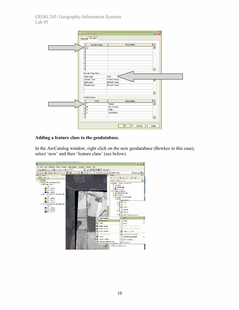
Right click on your geodatabase, select ‘properties’ and switch to the ‘domains’ tab.

Once there add a coded value text domain item called ‘LU’ directly into the empty box

and code in our four classes (your window should look like the one below). You will

need to click the “text” field to change it to “Domain” in the top window. Then, you will

click next to Domain in the lower window and select ‘LU’. Then you will start typing in

the Coded Values (Code: F, NF, etc. and the Description).


Lab 05

10

Adding a feature class to the geodatabase.

In the ArcCatalog window, right click on the new geodatabase (Bewkes in this case),

select ‘new’ and then ‘feature class’ (see below).


Lab 05

11

A new feature class wizard will pop up. Name the feature class LU36 and set type to

polygon features. Leave the alias blank (see below).

The next screen will ask you to select the coordinate system. We will take the easy

approach and import the coordinate system from the image we just rectified. To do this

click the import button and navigate to image you created above and click Add, followed

by Next. You should see the projection information from the layer you are importing at

the top. Once you see it, click OK. Accept the default when asked about the XY

tolerance.


Lab 05

12

Defining attributes of the feature class

Eventually, you will see a window similar to the one below. Basically this is where you

define the fields of an attribute table. For this tutorial, you only need to add the land

cover attribute (I called it Cover). This is confusing because you must type into the

empty cells below SHAPE and GEOMETRY (these are by default included in the table).

Make sure you indicate that this attribute should be attached to the LU Domain (i.e., you

are using the rules defined in the LU domain). In the example below, I selected a field

length of 16 to be sure there would be enough room for all the information I would put in

the attribute table. Click finish.

You should now be able to add this feature class on top of the registered 1936 photo, just

as you would a shapefile. Time to digitize.

Digitizing the Landcover

Open new empty map and add the newly georegistered Bewkes image.

Next, add the empty feature class you created for the 1936 landcover in the Bewkes

geodatabase. You must double click on the geodatabase icon (a cylinder) in order to see

the feature class. (You won’t see anything in the map view because the feature class

doesn’t yet include any features!) Also add the shapefile (Bewkesextent.shp) to your

map. This shapefile identifies the area we would like you to digitize. You might want to

only display the boundary of the polygon in order to see the imagery.

Make sure the Editor toolbar, shown below, is open (main GUI→ Customize→

Toolbars→ Editor).


Lab 05

13

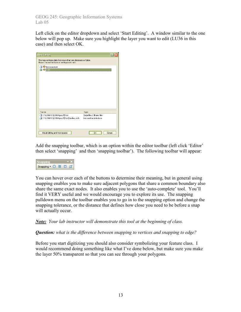
Left click on the editor dropdown and select ‘Start Editing’. A window similar to the one

below will pop up. Make sure you highlight the layer you want to edit (LU36 in this

case) and then select OK.

Add the snapping toolbar, which is an option within the editor toolbar (left click ‘Editor’

then select ‘snapping’ and then ‘snapping toolbar’). The following toolbar will appear:

You can hover over each of the buttons to determine their meaning, but in general using

snapping enables you to make sure adjacent polygons that share a common boundary also

share the same exact nodes. It also enables you to use the ‘auto-complete’ tool. You’ll

find it VERY useful and we would encourage you to explore its use. The snapping

pulldown menu on the toolbar enables you to go in to the snapping option and change the

snapping tolerance, or the distance that defines how close you need to be before a snap

will actually occur.

Note: Your lab instructor will demonstrate this tool at the beginning of class.

Question: what is the difference between snapping to vertices and snapping to edge?

Before you start digitizing you should also consider symbolizing your feature class. I

would recommend doing something like what I’ve done below, but make sure you make

the layer 50% transparent so that you can see through your polygons.


Lab 05

14

Note that I have symbolized ‘all other polygons’ as an obnoxious diagonal stripe. This is

because I want to see the polygons that are not labeled appropriately.

**NOTE**There are many tools available to you to actually do your onscreen digitizing.

Below we have highlighted a subset of them to get you started. Again, please consider

playing around with the various tools during the tutorial before moving on to the

exercise, and be sure to ask your lab instructor for help if you do not understand what you

are doing.**

The general routine involves drawing polygons around each of the individual landcover

types and labeling them appropriately. To do so you’ll need to know how to use a variety

of editing tools and will be learning how to turn your cursor into a variety of different

“tools”.

Creating new features (independent of others)

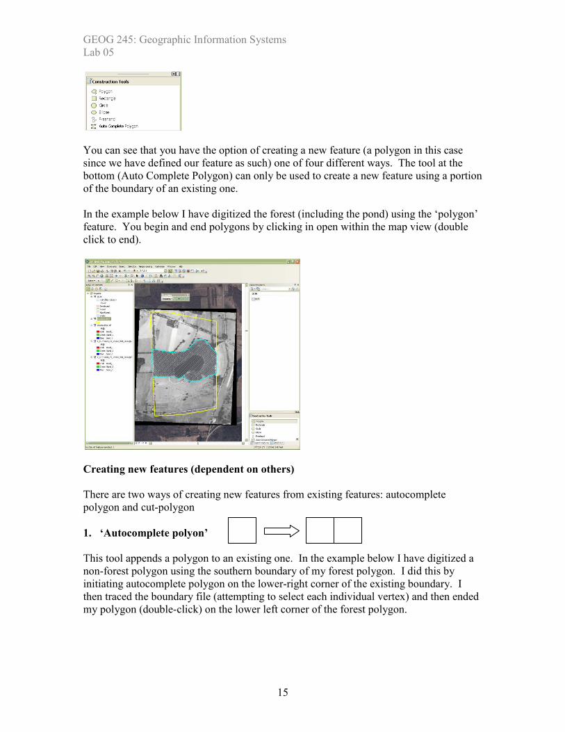
The ‘create features’ panel on the right side of the main ArcMap window should appear

once you start editing. The ‘Construction Tools’ at the bottom of this window (shown

below) are used to make new objects (as opposed to modifying existing ones).


Lab 05

15

You can see that you have the option of creating a new feature (a polygon in this case

since we have defined our feature as such) one of four different ways. The tool at the

bottom (Auto Complete Polygon) can only be used to create a new feature using a portion

of the boundary of an existing one.

In the example below I have digitized the forest (including the pond) using the ‘polygon’

feature. You begin and end polygons by clicking in open within the map view (double

click to end).

Creating new features (dependent on others)

There are two ways of creating new features from existing features: autocomplete

polygon and cut-polygon

1. ‘Autocomplete polyon’

This tool appends a polygon to an existing one. In the example below I have digitized a

non-forest polygon using the southern boundary of my forest polygon. I did this by

initiating autocomplete polygon on the lower-right corner of the existing boundary. I

then traced the boundary file (attempting to select each individual vertex) and then ended

my polygon (double-click) on the lower left corner of the forest polygon.


Lab 05

16

The advantage of this approach is that you do not have to duplicate the southern

boundary of the polygon existing polygon. And there will not be any slivers in between

them.

Question: why don’t you want any sliver polygons? Ask your lab instructor if you don’t

understand the answer.

2. Cut-polygon

The other way to create a new feature using an existing feature is to split a polygon in

two. This is exactly what is needed to pull out the lake from my forest polygon. First

you’ll need to select the polygon you want to split (or ‘cut’ to use ArcMap terminology).

You do this by making sure you are in the editing select mode (click the cursor shown by

the circle below). This is a different shaped arrow then the normal cursor (to turn

yourself into a normal cursor select the standard cursor button; see arrow below).


Lab 05

17

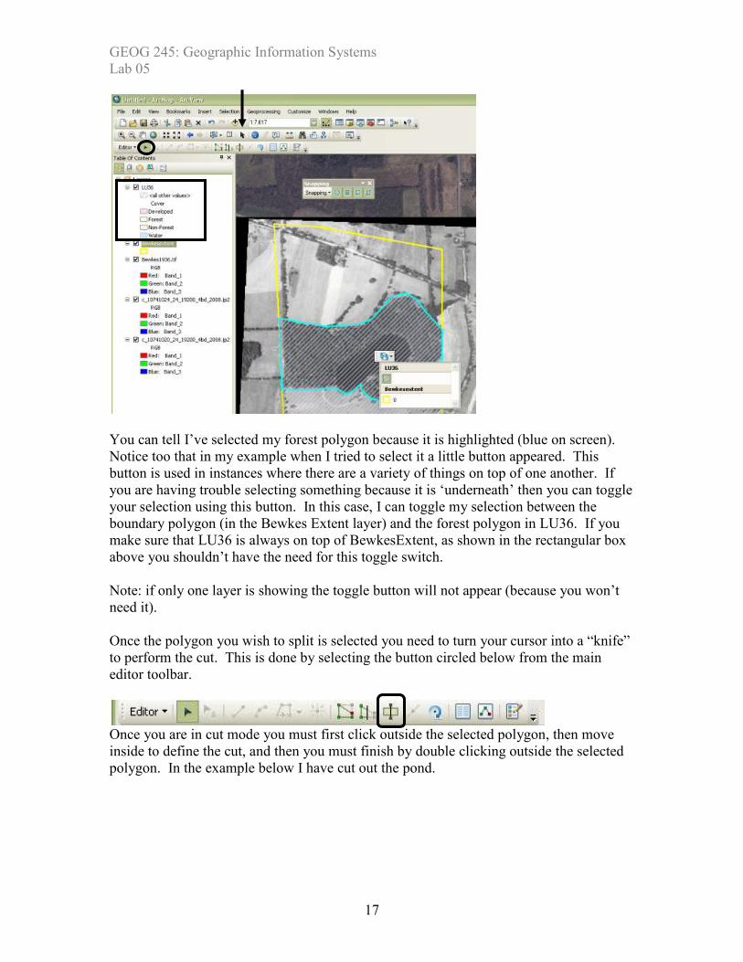
You can tell I’ve selected my forest polygon because it is highlighted (blue on screen).

Notice too that in my example when I tried to select it a little button appeared. This

button is used in instances where there are a variety of things on top of one another. If

you are having trouble selecting something because it is ‘underneath’ then you can toggle

your selection using this button. In this case, I can toggle my selection between the

boundary polygon (in the Bewkes Extent layer) and the forest polygon in LU36. If you

make sure that LU36 is always on top of BewkesExtent, as shown in the rectangular box

above you shouldn’t have the need for this toggle switch.

Note: if only one layer is showing the toggle button will not appear (because you won’t

need it).

Once the polygon you wish to split is selected you need to turn your cursor into a “knife”

to perform the cut. This is done by selecting the button circled below from the main

editor toolbar.

Once you are in cut mode you must first click outside the selected polygon, then move

inside to define the cut, and then you must finish by double clicking outside the selected

polygon. In the example below I have cut out the pond.


Lab 05

18

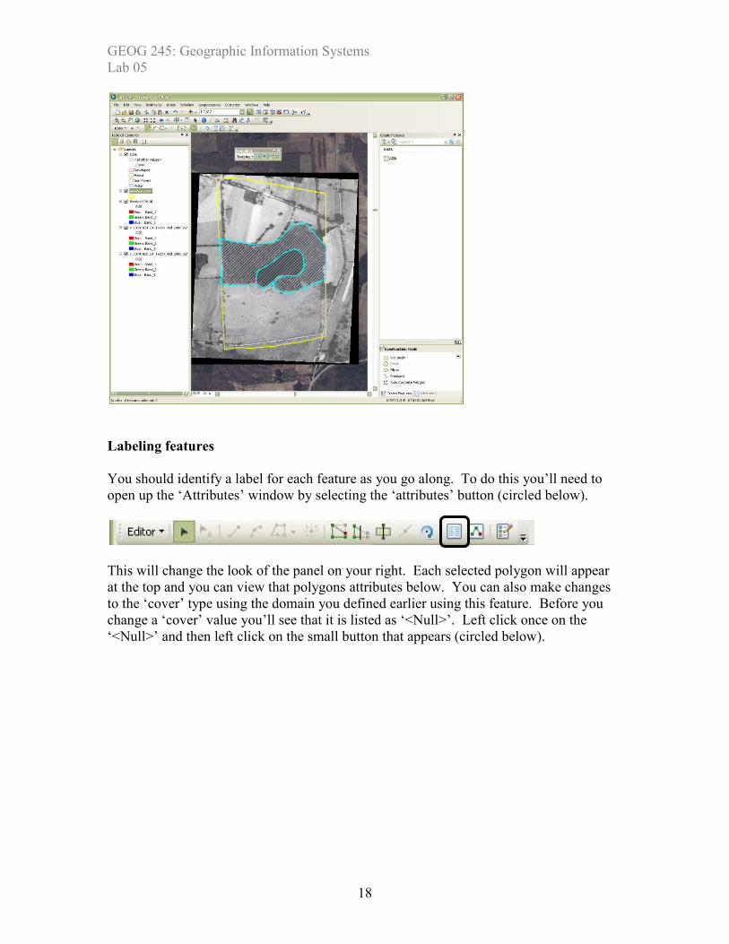
Labeling features

You should identify a label for each feature as you go along. To do this you’ll need to

open up the ‘Attributes’ window by selecting the ‘attributes’ button (circled below).

This will change the look of the panel on your right. Each selected polygon will appear

at the top and you can view that polygons attributes below. You can also make changes

to the ‘cover’ type using the domain you defined earlier using this feature. Before you

change a ‘cover’ value you’ll see that it is listed as ‘<Null>’. Left click once on the

‘<Null>’ and then left click on the small button that appears (circled below).


Lab 05

19

This will open a window like the one show in the example above. Here you define the

cover type of the polygon. In my example I am defining the pond polygon as ‘water’.

Once you define it the symbology should change it from vertical striped to blue.

If you have not symbolized the layer, this window will not appear.

“Donut-hole” polygons

You may find yourself in a situation where you need to draw a polygon within a polygon

in the same layer (do you follow?). Such a task does involve adding a new feature, but

that feature is neither purely independent nor dependent on existing polygons; thus, it

doesn’t fall into our two categories of creating new features.

If you simply added one it would be drawn on top of the existing polygon and you can’t

“cut” the existing polygon because that tool needs to be initiated and terminated outside

of a given polygon (just like it’s hard to use scissors to cut a hole in a the center of a

piece of paper).

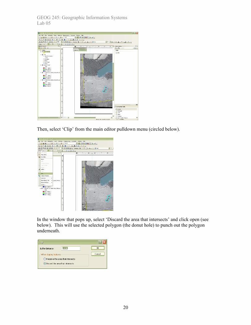
The way to deal with this is to initially draw a polygon on top of your existing one.

Below I have done just that to distinguish a group of trees in the middle of a field that I

want to call “forest”.


Lab 05

20

Then, select ‘Clip’ from the main editor pulldown menu (circled below).

In the window that pops up, select ‘Discard the area that intersects’ and click open (see

below). This will use the selected polygon (the donut hole) to punch out the polygon

underneath.


Lab 05

21

Modifying existing features

Sometimes you may find yourself in a situation where you need to modify the

edge of an existing polygon. For example below my ‘non-forest’ polygon’s

boundary doesn’t perfectly fit the study area (see circle). That is, it doesn’t share a

common boundary with BewkesExtent.

If you right click on a selected polygon that you want to modify you can select ‘Edit

vertices’. Doing so reveals the actual vertices; they will appear green on your screen.

Once revealed you can move existing ones as well as creating new ones by left clicking

on the line where you want to add one and selecting ‘insert vertex’. Then, you can move

them to make the BewkesExtent layer, thus assuring that you cover the entire study area

(and nothing else – don’t digitize outside). You will need to click outside the polygon to

enact the changes. Pay attention to the snapping information that appears when moving a

vertex to assure that you are actually snapping vertices in LU36 to those in

BewkesExtent.

Using a combination of the tools above complete your landcover map of the bewkes

center. Before you leave lab make sure you are comfortable with the process of

digitizing. The exercise will require you to perform a landcover classification on your

own.

6. Feature manipulation: dissolving (((((NOTES: fall 2012 – taken from Lab 7 (as

it seems more useful here)

Sometimes you’ll find yourself in a situation where you have many different neighboring

polygons that all have the same value. Since the polygons share a common boundary

there’s no reason why they can’t be dissolved together into one bigger polygon. This


Lab 05

22

situation is illustrated below which shows many different polygons with similar values

neighboring one another. This can happen frequently during digitizing depending on

which digitizing strategy you choose. For example, you may have had two non-forest

polygons next to each other during the heads-up digitizing lab. This can be easily fixed

by using the dissolve tool.

To demonstrate this tool we will dissolve the boundaries between all neighboring

landlocked countries in the world.

• Add a new dataframe and add the country.shp layer from the

C:\ESRI\ESRIDATA\World folder.

• Open up the attribute table. (What field would you use to select whether a

country was landlocked?) Symbolize by that attribute. Select by attribute based

on that field for landlocked countries. Fill in the blank: ____ countries out of a

total _____ are landlocked. Clear selection.

• Open the dissolve tool from the ArcToolbox (Data management tools

→Generalization → Dissolve). Select the proper Input Feature and

Dissolve_Field (the field by which the dissolve will be based). Once again, make

sure you save to an appropriate place and name your output file appropriately then

select ok.


Lab 05

23

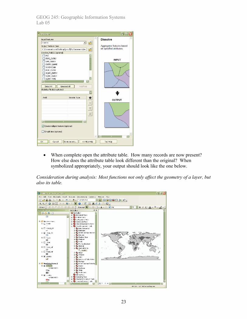
• When complete open the attribute table. How many records are now present?

How else does the attribute table look different than the original? When

symbolized appropriately, your output should look like the one below.

Consideration during analysis: Most functions not only affect the geometry of a layer, but

also its table.


Lab 05

24

tutorial 5 – heads-up digitizing in arcmap · to being saved. lab 5 imagery for this tutorial,...

Documents