gis lab: sorghum exercise arcmap 9 tutorial 2010.pdf · sorghum exercise – arcview 9 page 1 gis...

Sorghum Exercise – ArcView 9 page 1

GIS Lab: Sorghum Exercise – ArcMap 9

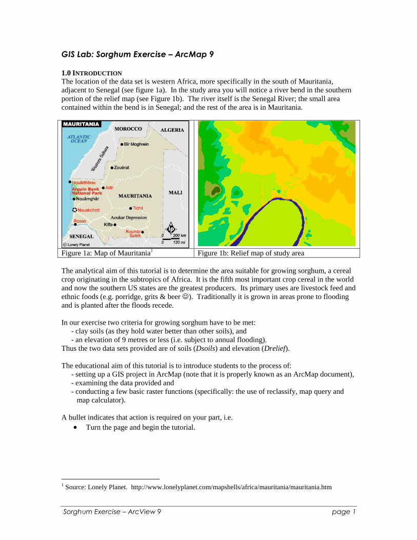
1.0 INTRODUCTION The location of the data set is western Africa, more specifically in the south of Mauritania,

adjacent to Senegal (see figure 1a). In the study area you will notice a river bend in the southern

portion of the relief map (see Figure 1b). The river itself is the Senegal River; the small area

contained within the bend is in Senegal; and the rest of the area is in Mauritania.

Figure 1a: Map of Mauritania1 Figure 1b: Relief map of study area

The analytical aim of this tutorial is to determine the area suitable for growing sorghum, a cereal

crop originating in the subtropics of Africa. It is the fifth most important crop cereal in the world

and now the southern US states are the greatest producers. Its primary uses are livestock feed and

ethnic foods (e.g. porridge, grits & beer ). Traditionally it is grown in areas prone to flooding

and is planted after the floods recede.

In our exercise two criteria for growing sorghum have to be met:

- clay soils (as they hold water better than other soils), and

- an elevation of 9 metres or less (i.e. subject to annual flooding).

Thus the two data sets provided are of soils (Dsoils) and elevation (Drelief).

The educational aim of this tutorial is to introduce students to the process of:

- setting up a GIS project in ArcMap (note that it is properly known as an ArcMap document),

- examining the data provided and

- conducting a few basic raster functions (specifically: the use of reclassify, map query and

map calculator).

A bullet indicates that action is required on your part, i.e.

Turn the page and begin the tutorial.

1 Source: Lonely Planet. http://www.lonelyplanet.com/mapshells/africa/mauritania/mauritania.htm


Estimated time to complete this lab: 50 minutes

2.0 INITIAL PROJECT SET-UP

This section covers the basic housekeeping chores of starting a map document:

1. copying the data to your directory

2. starting ArcGIS and adding these data to your new map document

3. activating the Spatial Analyst toolbar

4. setting the working directory (so the new data are saved to your directory)

5. saving the ArcMap document thus far.

2.1 Copy Data

The data for this project is in the folder Sorghum.

Copy the Sorghum folder to your U: drive. Rename the folder to

YourNameSorghum (i.e. CorrinSorghum).

2.2 Starting a New Project and Adding Data

Start ArcMap (click Start Programs ArcGIS ArcMap), on the next screen:

o Ensure the radio button for A new empty map is selected

o Ensure the Immediately add data check box indeed has a “check”

o Click OK

The Add Data window appears.


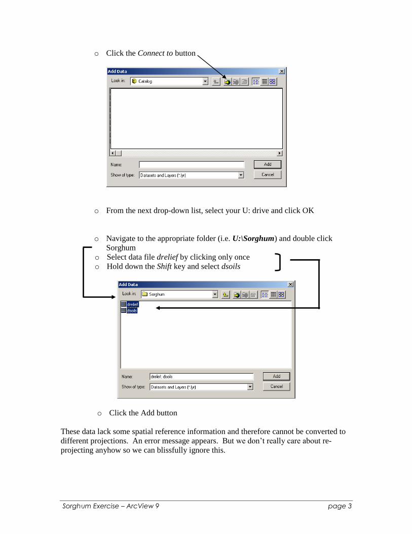
o Click the Connect to button

o From the next drop-down list, select your U: drive and click OK

o Navigate to the appropriate folder (i.e. U:\Sorghum) and double click

Sorghum

o Select data file drelief by clicking only once

o Hold down the Shift key and select dsoils

o Click the Add button

These data lack some spatial reference information and therefore cannot be converted to

different projections. An error message appears. But we don‟t really care about re-

projecting anyhow so we can blissfully ignore this.


Click OK

The Table of Contents section on the left side of the window should look similar (colours

for dsoils may vary – that‟s OK for now) to the following:

It is OK if the order of dsoils and drelief are reversed. However, you can click-and-drag

dsoils above drelief if you wish.

2.3 Enabling Spatial Analyst

As we will be working with raster grids we will need to „turn on‟ the Spatial Analyst

module.

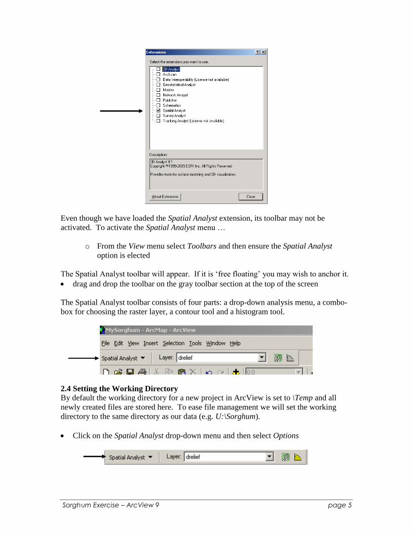
From the Tools menu select Extensions

o Ensure the Spatial Analyst check box has a tic mark and click the

button


Even though we have loaded the Spatial Analyst extension, its toolbar may not be

activated. To activate the Spatial Analyst menu …

o From the View menu select Toolbars and then ensure the Spatial Analyst

option is elected

The Spatial Analyst toolbar will appear. If it is „free floating‟ you may wish to anchor it.

drag and drop the toolbar on the gray toolbar section at the top of the screen

The Spatial Analyst toolbar consists of four parts: a drop-down analysis menu, a combo-

box for choosing the raster layer, a contour tool and a histogram tool.

2.4 Setting the Working Directory By default the working directory for a new project in ArcView is set to \Temp and all

newly created files are stored here. To ease file management we will set the working

directory to the same directory as our data (e.g. U:\Sorghum).

Click on the Spatial Analyst drop-down menu and then select Options


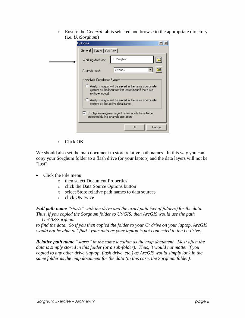
o Ensure the General tab is selected and browse to the appropriate directory

(i.e. U:\Sorghum)

o Click OK

We should also set the map document to store relative path names. In this way you can

copy your Sorghum folder to a flash drive (or your laptop) and the data layers will not be

“lost”.

Click the File menu

o then select Document Properties

o click the Data Source Options button

o select Store relative path names to data sources

o click OK twice

Full path name “starts” with the drive and the exact path (set of folders) for the data.

Thus, if you copied the Sorghum folder to U:/GIS, then ArcGIS would use the path

U:/GIS/Sorghum

to find the data. So if you then copied the folder to your C: drive on your laptop, ArcGIS

would not be able to “find” your data as your laptop is not connected to the U: drive.

Relative path name “starts” in the same location as the map document. Most often the

data is simply stored in this folder (or a sub-folder). Thus, it would not matter if you

copied to any other drive (laptop, flash drive, etc.) as ArcGIS would simply look in the

same folder as the map document for the data (in this case, the Sorghum folder).

U:\Sorghum


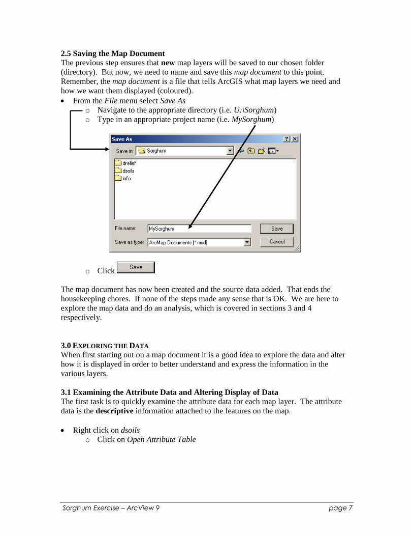
2.5 Saving the Map Document

The previous step ensures that new map layers will be saved to our chosen folder

(directory). But now, we need to name and save this map document to this point.

Remember, the map document is a file that tells ArcGIS what map layers we need and

how we want them displayed (coloured).

From the File menu select Save As

o Navigate to the appropriate directory (i.e. U:\Sorghum)

o Type in an appropriate project name (i.e. MySorghum)

o Click

The map document has now been created and the source data added. That ends the

housekeeping chores. If none of the steps made any sense that is OK. We are here to

explore the map data and do an analysis, which is covered in sections 3 and 4

respectively.

3.0 EXPLORING THE DATA

When first starting out on a map document it is a good idea to explore the data and alter

how it is displayed in order to better understand and express the information in the

various layers.

3.1 Examining the Attribute Data and Altering Display of Data The first task is to quickly examine the attribute data for each map layer. The attribute

data is the descriptive information attached to the features on the map.

Right click on dsoils

o Click on Open Attribute Table


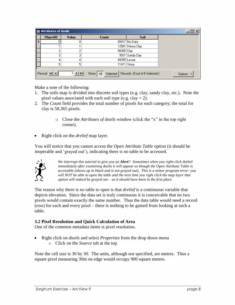
Make a note of the following:

1. The soils map is divided into discrete soil types (e.g. clay, sandy clay, etc.). Note the

pixel values associated with each soil type (e.g. clay = 2).

2. The Count field provides the total number of pixels for each category; the total for

clay is 58,365 pixels.

o Close the Attributes of dsoils window (click the “x” in the top right

corner).

Right click on the drelief map layer.

You will notice that you cannot access the Open Attribute Table option (it should be

inoperable and „grayed out‟), indicating there is no table to be accessed.

We interrupt this tutorial to give you an Alert!! Sometimes when you right-click drelief

immediately after examining dsoils it will appear as though the Open Attribute Table is

accessible (shows up in black and is not grayed out). This is a minor program error- you

will NOT be able to open the table and the next time you right click the map layer that

option will indeed be grayed out – as it should have been in the first place

The reason why there is no table to open is that drelief is a continuous variable that

depicts elevation. Since the data set is truly continuous it is conceivable that no two

pixels would contain exactly the same number. Thus the data table would need a record

(row) for each and every pixel – there is nothing to be gained from looking at such a

table.

3.2 Pixel Resolution and Quick Calculation of Area One of the common metadata items is pixel resolution.

Right click on dsoils and select Properties from the drop down menu

o Click on the Source tab at the top

Note the cell size is 30 by 30. The units, although not specified, are metres. Thus a

square pixel measuring 30m on edge would occupy 900 square metres.


Click OK to close the window.

Remember that the clay soil type was composed of 58,365 pixels. An estimate of area

would simply be:

Area = 58,365 pixels * 900 m2/pixel = 52,528,500 m

2

Area = 52,528,500 m2 / 10,000 m

2 /ha = 5,253 ha

3.3 Viewing a Histogram of Pixel Values You will recall that we could not open an attribute table for the theme drelief. We can,

however, look at the frequency distribution of the pixel values.

In the Layer drop down box on the Spatial Analyst toolbar select drelief.

o Then click the histogram button

Note the distribution is shaded with the same gray scale colours as used in the legend.


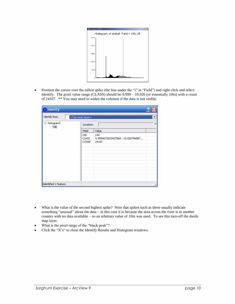
Position the cursor over the tallest spike (the line under the “i” in “Field”) and right click and select

Identify. The pixel value range (CLASS) should be 9.999 – 10.026 (or essentially 10m) with a count

of 24107. ** You may need to widen the columns if the data is not visible.

What is the value of the second highest spike? Note that spikes such as these usually indicate

something “unusual” about the data – in this case it is because the area across the river is in another

country with no data available – so an arbitrary value of 10m was used. To see this turn-off the dsoils

map layer.

What is the pixel range of the “black peak”?

Click the “X‟s” to close the Identify Results and Histogram windows.


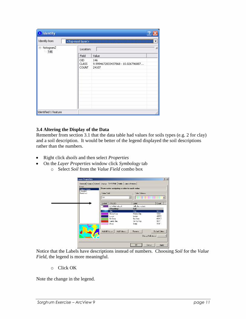
3.4 Altering the Display of the Data Remember from section 3.1 that the data table had values for soils types (e.g. 2 for clay)

and a soil description. It would be better of the legend displayed the soil descriptions

rather than the numbers.

Right click dsoils and then select Properties

On the Layer Properties window click Symbology tab

o Select Soil from the Value Field combo box

Notice that the Labels have descriptions instead of numbers. Choosing Soil for the Value

Field, the legend is more meaningful.

o Click OK

Note the change in the legend.


Colours for discrete data sets are chosen at random. Controlling colours can highlight

data types of interest – in our case we are interested in clay soils.

Click on the colour box to the left of „clay‟ in the Table of Contents

A Color Selector box will appear.

o Click on the pink color in the „rainbow bar‟

o Click OK

Using the same procedure set the colours as follows: Heavy Clay – purple, Levee –

brown, No Data – black, Sandy Clay – medium green, Stony – dark green.

Next we will alter the display of drelief. However, in order to view any changes, we will

need to turn off the dsoils map layer, since it displays on top of drelief.

Click the box next to dsoils to turn off its display (there should be no tic mark)

Click on the black & white colour bar under drelief


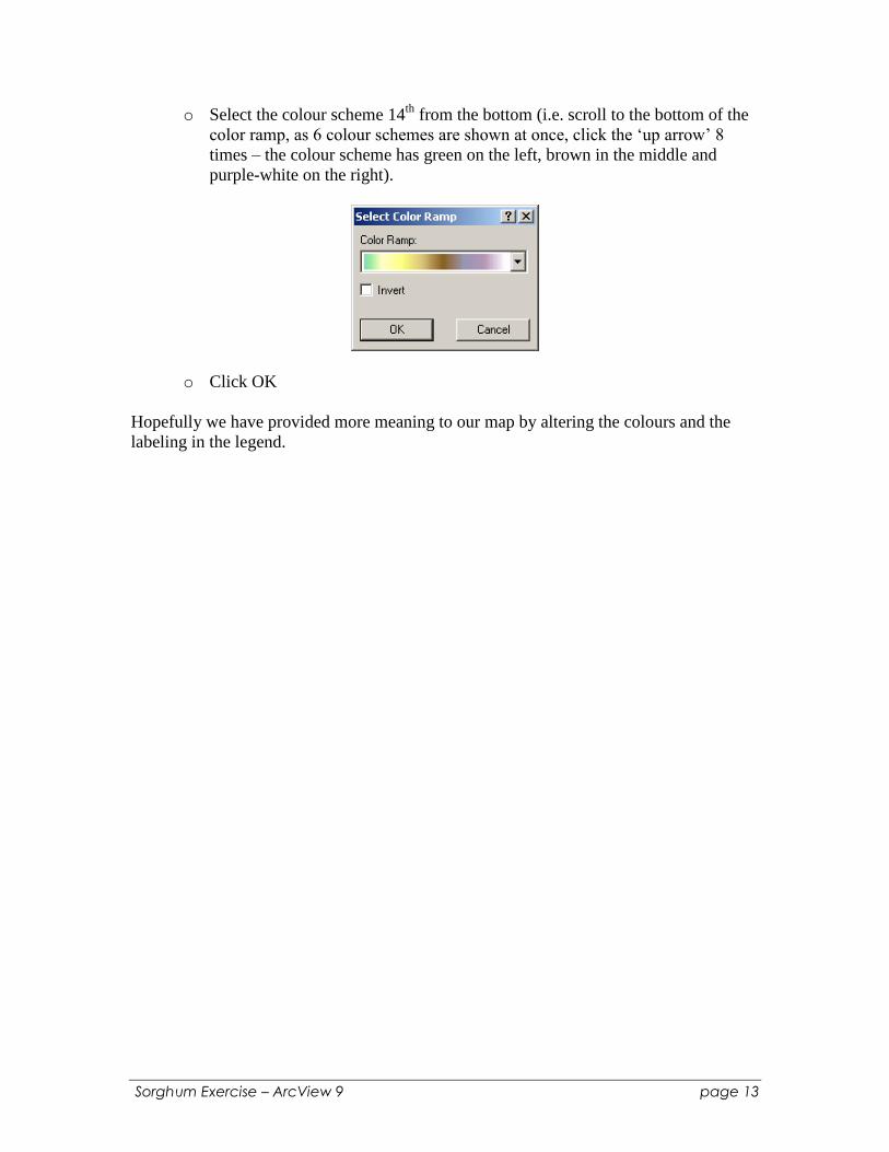
o Select the colour scheme 14th

from the bottom (i.e. scroll to the bottom of the

color ramp, as 6 colour schemes are shown at once, click the „up arrow‟ 8

times – the colour scheme has green on the left, brown in the middle and

purple-white on the right).

o Click OK

Hopefully we have provided more meaning to our map by altering the colours and the

labeling in the legend.


4.0 DETERMINING THE COINCIDENT AREA

The analytical task is a simple one: find the area where both of the following conditions

occur:

- clay soils, and

- elevation ≤ 9 meters.

This is known as constraint mapping (or restrictive modeling) and, prior to the advent of

a more versatile and functional interface, required several steps. The following is a brief

overview of the steps required.

Phase 1: Create Boolean (Logic) Layers

The first phase is creating Boolean (or logic) layers from the raw data layers. A

Boolean layer contains pixels with values of only 0‟s and 1‟s, whereby the 1‟s

indicate areas that meet our criteria and 0‟s do not. A Boolean layer is created for

each parameter of interest. In our case we would create two Boolean layers:

1. one from Dsoils, where 1‟s would indicate clay and 0‟s would indicate all

other soil types, and

2. a second from Drelief, where 1‟s would indicate an elevation of 9 or less

(i.e. the flood area) and 0‟s for all higher ground

Phase 2: Combine Boolean Layers

The second phase involves combining the Boolean layers in such a way that the

resultant layer would have 1‟s only where all the parameters are satisfied. In our

case this means that the soil type is clay and the elevation is less than or equal to 9

meters.

We will now determine the area that is suitable for growing sorghum. We have a few

options for conducting this analysis. As the objective of the exercise is to learn about

raster functionality and become familiar with the Spatial Analyst interface, we will

conduct the analysis two different ways. Luckily each method will only take a few

minutes.

4.1 The “Old Way”: Creating Intermediate Data Layers As previously described, it can take several steps to complete a simple operation.

Normally this is not done today, unless there is value in producing the intermediate raster

layers. We will complete the task „the old way‟ to ensure we understand exactly what is

happening and to gain exposure to several raster functions.

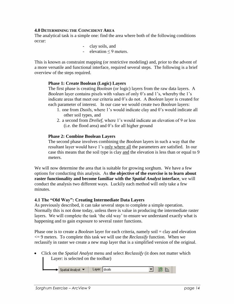
Phase one is to create a Boolean layer for each criteria, namely soil = clay and elevation

<= 9 meters. To complete this task we will use the Reclassify function. When we

reclassify in raster we create a new map layer that is a simplified version of the original.

Click on the Spatial Analyst menu and select Reclassify (it does not matter which

Layer: is selected on the toolbar)


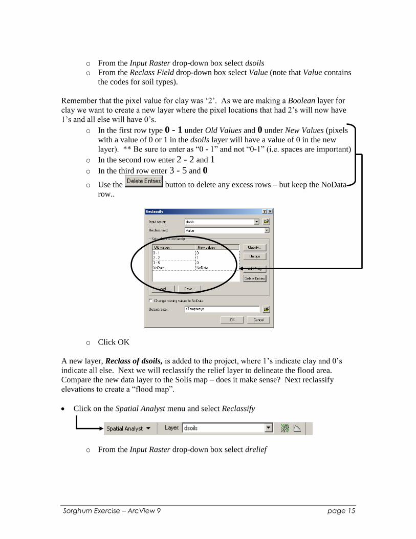
o From the Input Raster drop-down box select dsoils

o From the Reclass Field drop-down box select Value (note that Value contains

the codes for soil types).

Remember that the pixel value for clay was „2‟. As we are making a Boolean layer for

clay we want to create a new layer where the pixel locations that had 2‟s will now have

1‟s and all else will have 0‟s.

o In the first row type 0 - 1 under Old Values and 0 under New Values (pixels

with a value of 0 or 1 in the dsoils layer will have a value of 0 in the new

layer). ** Be sure to enter as “0 - 1” and not “0-1” (i.e. spaces are important)

o In the second row enter 2 - 2 and 1

o In the third row enter 3 - 5 and 0

o Use the button to delete any excess rows – but keep the NoData

row..

o Click OK

A new layer, Reclass of dsoils, is added to the project, where 1‟s indicate clay and 0‟s

indicate all else. Next we will reclassify the relief layer to delineate the flood area.

Compare the new data layer to the Solis map – does it make sense? Next reclassify

elevations to create a “flood map”.

Click on the Spatial Analyst menu and select Reclassify

o From the Input Raster drop-down box select drelief


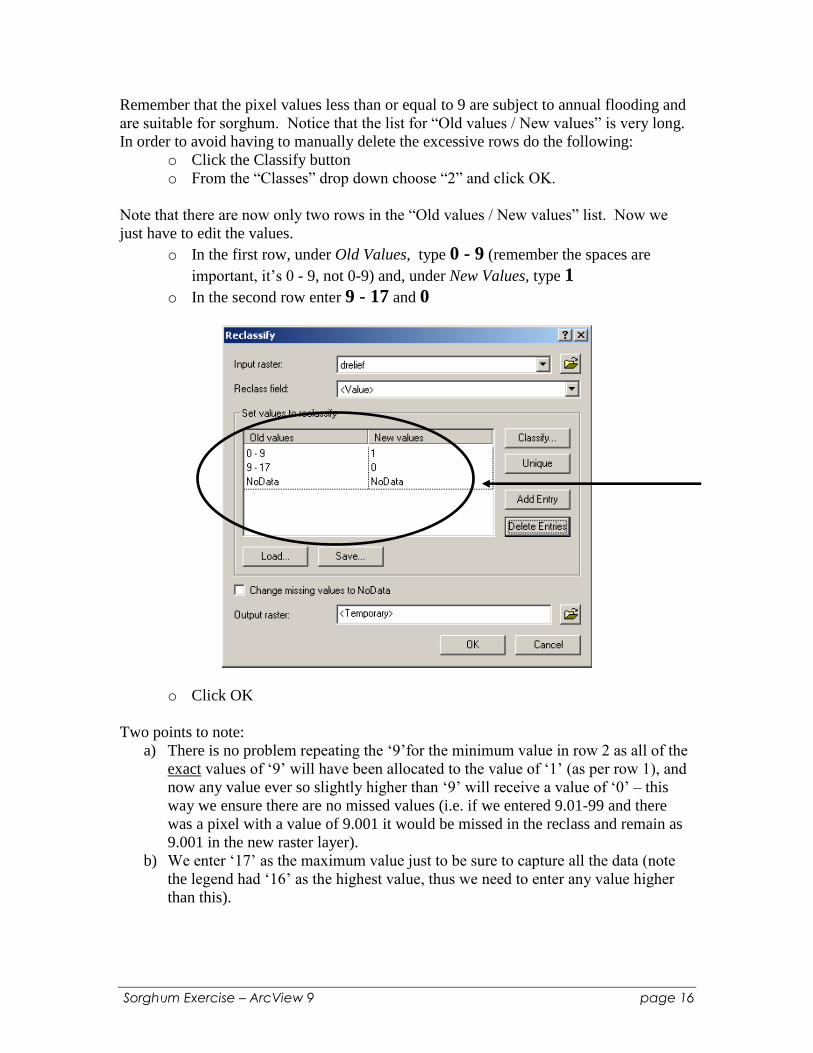
Remember that the pixel values less than or equal to 9 are subject to annual flooding and

are suitable for sorghum. Notice that the list for “Old values / New values” is very long.

In order to avoid having to manually delete the excessive rows do the following:

o Click the Classify button

o From the “Classes” drop down choose “2” and click OK.

Note that there are now only two rows in the “Old values / New values” list. Now we

just have to edit the values.

o In the first row, under Old Values, type 0 - 9 (remember the spaces are

important, it‟s 0 - 9, not 0-9) and, under New Values, type 1

o In the second row enter 9 - 17 and 0

o Click OK

Two points to note:

a) There is no problem repeating the „9‟for the minimum value in row 2 as all of the

exact values of „9‟ will have been allocated to the value of „1‟ (as per row 1), and

now any value ever so slightly higher than „9‟ will receive a value of „0‟ – this

way we ensure there are no missed values (i.e. if we entered 9.01-99 and there

was a pixel with a value of 9.001 it would be missed in the reclass and remain as

9.001 in the new raster layer).

b) We enter „17‟ as the maximum value just to be sure to capture all the data (note

the legend had „16‟ as the highest value, thus we need to enter any value higher

than this).


A new layer, Reclass of drelief, is added to the project, where 1‟s indicate flood area

(less than or equal to 9m) and 0‟s indicate non-flood areas (i.e. higher ground).

Next we need to combine these two Boolean layers to delineate areas where both criteria

are met (i.e. where the 1‟s overlap).

Click on the Spatial Analyst menu and select Raster Calculator

o From the Layers double click Reclass of drelief

o Click the button

o From the Layers double click Reclass of dsoils

It is understood that

([Reclass of drelief] & [Reclass of dsoils]) is equivalent to

([Reclass of drelief = 1] and [Reclass of dsoils = 1]).

What this means is that the new map layer will have 1‟s where the soils were clay and

flooded.

Please note that it is very important to get the „syntax‟ of the expression exact – if not, a

“Syntax Error” message will appear. Syntax errors are usually not obvious. To correct

the situation it is easiest to close the Raster Calculator window and then reselect it from

the menu and begin fresh.

o Click the „Evaluate‟ button

A new raster layer is added to the project, entitled Calculation. On this layer the 1‟s

represent areas suitable for growing sorghum, where clay soils and elevations <= 9

metres coincide.


As we only had two criteria, the „old way‟ requires only 3 steps: the creation of two

Boolean layers and the overlay of these two layers. This process exposed us to two

functions:

- Reclass: which is used to simplify a raster data set (can be into Boolean with only

1‟s and 0‟s, or it could also be used to put continuous data, such as elevation, into

classes)

- Raster Calculator: which can be used to combine layers.

To aid in discerning the results from other approaches we will rename this theme “Old

Way”

Right-click on this newly created theme Calculation and select Properties

o Select the General tab

o In the Layer Name box type Old Way.

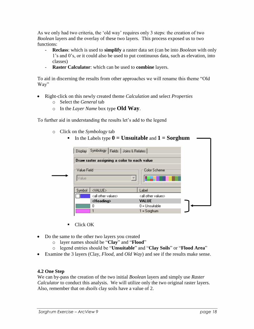
To further aid in understanding the results let‟s add to the legend

o Click on the Symbology tab

In the Labels type 0 = Unsuitable and 1 = Sorghum

Click OK

Do the same to the other two layers you created

o layer names should be “Clay” and “Flood”

o legend entries should be “Unsuitable” and “Clay Soils” or “Flood Area”

Examine the 3 layers (Clay, Flood, and Old Way) and see if the results make sense.

4.2 One Step We can by-pass the creation of the two initial Boolean layers and simply use Raster

Calculator to conduct this analysis. We will utilize only the two original raster layers.

Also, remember that on dsoils clay soils have a value of 2.


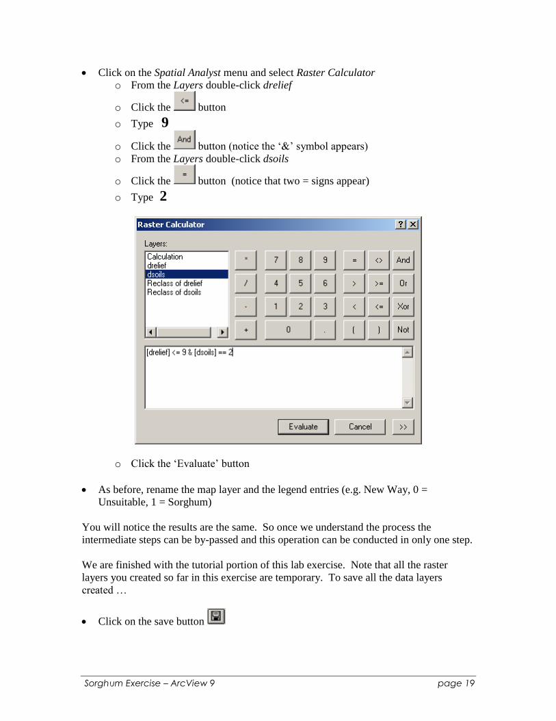
Click on the Spatial Analyst menu and select Raster Calculator

o From the Layers double-click drelief

o Click the button

o Type 9

o Click the button (notice the „&‟ symbol appears)

o From the Layers double-click dsoils

o Click the button (notice that two = signs appear)

o Type 2

o Click the „Evaluate‟ button

As before, rename the map layer and the legend entries (e.g. New Way, 0 =

Unsuitable, 1 = Sorghum)

You will notice the results are the same. So once we understand the process the

intermediate steps can be by-passed and this operation can be conducted in only one step.

We are finished with the tutorial portion of this lab exercise. Note that all the raster

layers you created so far in this exercise are temporary. To save all the data layers

created …

Click on the save button


5.0 SUMMARY When setting up a map document in ArcMap one of first the issues that needs to be

addressed is that of file management. A project can utilize data from a variety of

locations. There are three issues to contend with: the „raw‟ source data (e.g. Dsoils),

newly generated data (Old Way), and the project itself (MySorghum). For simple projects

it is often most convenient to locate all data in one directory (folder). This requires three

steps:

Create a project folder and copy source data to it, OR make a copy of the data

folder

Set the working directory to this same directory (folder) so newly generated data

is created here, and

Save the project to the same directory.

Setting relative path names will allow you to copy your folder (with your data and map

document to another source) to another location with issues of „lost data layers‟.

When first starting a project it is necessary to be familiar with the data. Changing the

way data is displayed can make the map more meaningful. Take for example the soils

data; its legend displayed the pixel values. These numbers had little meaning, but by

changing the legend to display soil types the map became more informative.

The analysis just conducted can be considered a spatial query with two criteria,

specifically – “where is the area where clay soils and an elevation of 9 metres or less

coincide?” A spatial query can be conducted with many criteria. For this type of

analysis each criteria has two categories: area that satisfies the criteria and area that does

not. If it were useful to create intermediate layers, it is standard to use 1‟s for satisfactory

area (i.e. meets the criteria) and 0‟s for unsatisfactory areas. Such a layer with only 1‟s

and 0‟s is known as a logic, or Boolean layer. The final step is to query for where 1‟s

occur in all the Boolean layers. As experienced in this exercise, this type of analysis can

also be accomplished in only one step, by-passing the creation of the intermediate layers.

Now, you are ready to perform the assignment portion of this lab. Good luck!

gis lab: sorghum exercise arcmap 9 tutorial 2010.pdf · sorghum exercise – arcview 9 page 1 gis...

Documents