tuning of scattering properties by periodic modulation
TRANSCRIPT

Tuning of Scattering Properties byPeriodic Modulation
Diplomarbeitin
Theoretischer Physik
vonChristoph Dauer
durchgeführt amFachbereich Physik
der Technischen Universität Kaiserslautern
unter Anleitung vonProf. Dr. Sebastian Eggert
April 2018


Abstract
Periodic driving of quantum systems gives rise to novel and exciting phenomena. In recent experi-ments the interaction of particles in a Bose-Einstein condensate has been altered time periodicallyand as a result the excitation of collective modes has been observed without changing the condensatetrap [1]. Furthermore, the emergence of the collective emission of matter-wave jets from a drivencondensate has been detected [2].
The aim of this thesis is to observe, how the scattering of particles can be tuned by periodic driving.Therefore, we investigate the two-body problem with a time-periodic interaction potential [3–5]. Bythe use of Floquet theory the Floquet-partial wave expansion is derived. It is capable of calculatingcross sections and steady-state wave functions for scattering by a time-periodic potential. We applythis method to a sinusoidally driven contact potential, which describes the two-body interaction ofquantum particles in the regime of s-wave scattering. In this case it is possible to map the drivenscattering problem on a recursion relation connecting different Fourier components of the steady-state wave function. By solving this recursion we obtain a time-averaged scattering amplitude andobserve resonances, which permit to tune this scattering amplitude to very large positive or negativevalues, signalling strong enhancement of scattering induced by time-periodic driving. The width ofthese resonances can be tuned by the driving strength, while the frequency of the drive allows oneto control the actual enhancement of scattering. We find position and width of these resonances fora large range of driving strengths and spot that inelastic scattering is suppressed in their vicinity.We can explain these resonances by the phenomenon of Fano resonance involving a bound state inthe continuum. In addition, we find a Kramers-Kronig like relation connecting real and imaginarypart of the time-averaged scattering amplitude and demonstrate that the shape of these resonancescan be approximately described by a two-channel model. Using the Floquet-partial wave expansionin its full extend, we are finally able to overcome the restriction of sinusoidal driving and investigatethe influence of higher-Fourier components of the driven contact potential on the resonances.
A possible experimental realisation of our model is a periodically driven magnetic Feshbach res-onance [3], which grants the creation of resonances at magnetic field strengths beside the actualmagnetic Feshbach resonance. Our method is able to predict the enhancement of scattering in thissetting in a wide range of driving strengths.


Zusammenfassung
Periodisch getriebene Quantensysteme weisen neuartige und interessante Phänomene auf. In ver-schiedenen Experimenten wurde die Wechselwirkungsstärke von Teilchen in einem Bose-EinsteinKondensat zeitlich moduliert [1,2]. Dies führt einerseits zur Anregung kollektiver Moden, ohne dassÄnderungen an der Falle vorgenommen werden müssen [1], andererseits wurde das Auftreten kollek-tiver Emissionen von Materiewellen beobachtet [2].
Das Ziel dieser Arbeit besteht darin, zu untersuchen, wie die Streuung von Teilchen mit Hilfe zeitlichperiodischen Treibens verändert werden kann. Daher wird das Zweikörperproblem mit einem zeitlichperiodisch modulierten Wechselwirkungspotential [3–5] betrachtet. Mit Hilfe der Floquet-Theoriewird die Floquet-Partialwellenentwicklung hergeleitet, welche die Berechnung von Streuquerschnit-ten und Wellenfunktionen für beliebig zeitlich periodisch modulierte Potentiale ermöglicht. DieseMethode wird auf ein harmonisch moduliertes Kontaktpotential angewendet, welches die Zweikör-perwechselwirkung in der Näherung der s-Wellen Streuung beschreibt. In diesem Fall ist es möglich,das getriebene Streuproblem auf eine Rekursionsrelation zu transformieren. Die Lösung jener Rekur-sionsrelation, welche verschiedene Fourierkomponenten der Wellenfunktion verknüpft, erlaubt dieBerechnung der zeitgemittelten Streuamplitude. Es treten Resonanzen auf, welche es ermöglichen,die Streuamplitude zu sehr großen positiven oder negativen Werten einzustellen und dadurch zueiner starken Erhöhung der Streurate zu führen. Die Breite dieser Resonanzen kann mit Hilfeder Treibamplitude eingestellt werden, während die Treibfrequenz die tatsächliche Erhöhung derStreuamplitude bestimmt. Wir ermitteln Position und Breite dieser Resonanzen für einen großenBereich von Treibamplituden und beobachten, dass inelastische Streuung in der Nähe der Reso-nanz unterdrückt ist. Das Auftreten der Resonanzen wird durch das Phänomen der Fano-Resonanzerklärt. Zusätzlich stellen wir fest, dass Real- und Imaginärteil der Streuamplitude durch eine Re-lation, die den Kramers-Kronig Beziehungen ähnelt, verknüpft sind und zeigen, dass die Form derResonanz durch ein Zweikanalmodell angenähert werden kann. Unter Verwendung der Floquet-Partialwellenentwicklung sind wir letztendlich in der Lage, die Restriktion des sinusartigen Treibenszu verlassen und die Auswirkungen höherer Fourierkomponenten des zeitlich periodisch moduliertenKontaktpotentials zu untersuchen.
Eine mögliche experimentelle Realisierung unseres Modells ist die periodisch getriebene magnetischeFeshbach-Resonanz [3]. Diese erlaubt die Erhöhung der Streuamplitude in einem weiten Bereichum die eigentliche magnetische Feshbach-Resonanz. Unsere Methode erlaubt die Vorhersage vonResonanzen für ein großes Spektrum an Treibamplituden.


Contents
1. Introduction 11.1. Periodic Driving in Physical Systems . . . . . . . . . . . . . . . . . . . . . . . . . . . 11.2. Tuning the Interaction in Ultracold Gases . . . . . . . . . . . . . . . . . . . . . . . . 31.3. Tuning the Interaction Strength by Periodic Driving . . . . . . . . . . . . . . . . . . . 31.4. Outline of the Thesis . . . . . . . . . . . . . . . . . . . . . . . . . . . . . . . . . . . . 5
2. Scattering Theory 72.1. Introduction . . . . . . . . . . . . . . . . . . . . . . . . . . . . . . . . . . . . . . . . . 72.2. Asymptotic Form and Scattering Quantities . . . . . . . . . . . . . . . . . . . . . . . 7
2.2.1. Partial Wave Expansion . . . . . . . . . . . . . . . . . . . . . . . . . . . . . . 82.2.2. Scattering Length . . . . . . . . . . . . . . . . . . . . . . . . . . . . . . . . . . 10
2.3. Scattering by a Hard-Sphere Potential . . . . . . . . . . . . . . . . . . . . . . . . . . 11
3. Feshbach Resonances 133.1. Introduction to Feshbach Resonances . . . . . . . . . . . . . . . . . . . . . . . . . . . 133.2. Feshbach Resonances in Ultracold Quantum Gases . . . . . . . . . . . . . . . . . . . . 15
3.2.1. Magnetic Feshbach Resonance . . . . . . . . . . . . . . . . . . . . . . . . . . . 163.2.2. Optical Feshbach Resonance . . . . . . . . . . . . . . . . . . . . . . . . . . . . 163.2.3. Microwave- and Radio Frequency induced Feshbach Resonances . . . . . . . . 173.2.4. Driving Induced Scattering Resonance . . . . . . . . . . . . . . . . . . . . . . 18
4. Floquet Theory 214.1. Floquet Theorem . . . . . . . . . . . . . . . . . . . . . . . . . . . . . . . . . . . . . . 214.2. Floquet Equation and Properties of Floquet Modes . . . . . . . . . . . . . . . . . . . 224.3. Time Evolution and Effective Hamiltonian . . . . . . . . . . . . . . . . . . . . . . . . 24
5. Floquet-Scattering Theory 275.1. Coupled-Channel Equations and Cross Sections . . . . . . . . . . . . . . . . . . . . . 27
5.1.1. Coupled-Channel Equations . . . . . . . . . . . . . . . . . . . . . . . . . . . . 275.1.2. Asymptotic Waveform . . . . . . . . . . . . . . . . . . . . . . . . . . . . . . . 285.1.3. Cross Section . . . . . . . . . . . . . . . . . . . . . . . . . . . . . . . . . . . . 30
5.2. Floquet-Partial Wave Expansion . . . . . . . . . . . . . . . . . . . . . . . . . . . . . . 325.2.1. Radial-Floquet Equation . . . . . . . . . . . . . . . . . . . . . . . . . . . . . . 325.2.2. Scattering Amplitudes in Floquet-Partial Wave Expansion . . . . . . . . . . . 335.2.3. Floquet-Optical Theorem . . . . . . . . . . . . . . . . . . . . . . . . . . . . . 37
5.3. Indistinguishable Particles . . . . . . . . . . . . . . . . . . . . . . . . . . . . . . . . . 38
i

Contents
6. Contact Potential with Driven Scattering Length 416.1. Driven Contact Potential . . . . . . . . . . . . . . . . . . . . . . . . . . . . . . . . . . 416.2. Derivation of Recursion Relation . . . . . . . . . . . . . . . . . . . . . . . . . . . . . 436.3. Scale Invariance of Recursion . . . . . . . . . . . . . . . . . . . . . . . . . . . . . . . 466.4. Solution Methods for the Recursion Relation . . . . . . . . . . . . . . . . . . . . . . . 47
6.4.1. Truncation to Linear Set of Equations . . . . . . . . . . . . . . . . . . . . . . 486.4.2. Limit of Large Driving Frequencies . . . . . . . . . . . . . . . . . . . . . . . . 486.4.3. Limit of Low Driving Frequencies . . . . . . . . . . . . . . . . . . . . . . . . . 50
7. Enhancement of Scattering by Periodic Driving 537.1. Overview . . . . . . . . . . . . . . . . . . . . . . . . . . . . . . . . . . . . . . . . . . . 537.2. Feshbach-Fano Physics in Floquet Picture . . . . . . . . . . . . . . . . . . . . . . . . 577.3. Investigation of Resonance Positions . . . . . . . . . . . . . . . . . . . . . . . . . . . 62
7.3.1. Numerical Calculation . . . . . . . . . . . . . . . . . . . . . . . . . . . . . . . 627.3.2. Analytic Evaluation . . . . . . . . . . . . . . . . . . . . . . . . . . . . . . . . . 64
7.4. Scattering Amplitude in the Vicinity of a Resonance . . . . . . . . . . . . . . . . . . . 687.4.1. Frequency Controlled Feshbach Scattering Amplitude . . . . . . . . . . . . . . 687.4.2. Scattering Amplitude of a Simple Coupled Channel Model . . . . . . . . . . . 72
7.5. Position and Width of Scattering Resonances . . . . . . . . . . . . . . . . . . . . . . . 757.5.1. Energy Dependence of Parameters . . . . . . . . . . . . . . . . . . . . . . . . . 757.5.2. Position and Width in the ω-a1 Plane . . . . . . . . . . . . . . . . . . . . . . . 787.5.3. Relation to Simple Coupled Channel Model . . . . . . . . . . . . . . . . . . . 80
7.6. Kramers-Kronig like Relation between Real and Imaginary Part . . . . . . . . . . . . 837.7. Scattering Amplitude at Large Driving Frequencies . . . . . . . . . . . . . . . . . . . 857.8. Scattering Amplitude at Low Driving Frequencies . . . . . . . . . . . . . . . . . . . . 86
8. Influence of Higher Fourier Modes of the Driven Potential 898.1. Contact Potential with General Time-Periodic Driving . . . . . . . . . . . . . . . . . 898.2. Commensurate Two Colour Drive . . . . . . . . . . . . . . . . . . . . . . . . . . . . . 918.3. Periodically Driven Magnetic Feshbach Resonance . . . . . . . . . . . . . . . . . . . . 948.4. Frequency and Length Scale for Scattering of Ultracold Atoms . . . . . . . . . . . . . 96
9. Conclusion and Outlook 999.1. Conclusion . . . . . . . . . . . . . . . . . . . . . . . . . . . . . . . . . . . . . . . . . . 999.2. Outlook . . . . . . . . . . . . . . . . . . . . . . . . . . . . . . . . . . . . . . . . . . . 100
9.2.1. Periodically Driven Optical Feshbach Resonance . . . . . . . . . . . . . . . . . 1019.2.2. Scattering in Quantum Gases with Internal Degree of Freedom . . . . . . . . . 1039.2.3. Driven Impurities in Coupled Wave-Guide Arrays . . . . . . . . . . . . . . . . 104
Appendices 105
A. Contact Potential 107A.1. Scattering by a Contact Potential . . . . . . . . . . . . . . . . . . . . . . . . . . . . . 108A.2. Bound State . . . . . . . . . . . . . . . . . . . . . . . . . . . . . . . . . . . . . . . . . 109
B. Kramers-Kronig Relations for Anti-Causal Susceptibilities 111
ii

Contents
C. Derivation of Scattering Amplitude of a Simple Coupled-Channel Model 113
D. Limit of Vanishing γ of Approximative Formula (7.54) 117
E. Gross-Pitaevskii Equation with Time Dependent Interaction Strength 119E.1. Derivation of a Gross-Pitaevskii Equation . . . . . . . . . . . . . . . . . . . . . . . . 119E.2. Continuity Equation and Effect of Imaginary Scattering Length . . . . . . . . . . . . 120
Bibliography 121
iii


1. Introduction
Although Floquet theory is well established in research dealing with atoms in strong laser fields[6–10], it is in the recent time introduced to various areas of physics in order to describe and proposeperiodically driven systems with interesting and novel properties. We therefore give in Section 1.1an overview of driven physical systems and how properties of these systems can be tuned by periodicdriving. Section 1.2 provides a short introduction into the tuning of the inter-particle interactionsin ultracold quantum gases. Section 1.3 combines both previous Sections and gives a short insightinto the setting of our thesis. Section 1.4 is devoted to the outline of the thesis.
1.1. Periodic Driving in Physical Systems
Periodic driving of physical systems gives rise to exciting novel phenomena. A simple and impressingexample is the Kapitza pendulum [11–13]. As drawn in Figure 1.1, it consists of a rigid pendulumpossessing a pivot, which vibrates in vertical direction. If the vibration is performed with a largeenough frequency and amplitude, a counter intuitive behaviour is observed: The upper equilibrium,where the pendulum is inverted, becomes stable and the lower unstable. Kapitza understood thisbehaviour by separating the angular motion in a fast oscillation and a slow movement. Averagingout the fast motion leads to an effective potential stabilizing the slowly varying angular degree offreedom in the upper equilibrium.
Also in quantum mechanics periodic driving is used in order to induce a behaviour, which is notpresent in the static case. A simple band structure can be described by the tight-binding model [14]on a lattice. It consists of an array of lattice sites, which are connected by the hopping amplitude J .The hopping amplitude J can be seen as the matrix element for a transition between neighbouringlattice sites. If a time-periodic field with strength E and frequency ω, which is large in comparison tothe bandwidth of the lattice, is applied, the driven system behaves like a static lattice with effectivehopping amplitude [15]
Jeff = JJ0
(E~ω
), (1.1)
which is normalised by the Bessel function of order zero J0(x). The effective hopping amplitudedepends explicitly on the driving strength E and driving frequency ω and can therefore be tunedby periodic driving. This has been exploited in order to investigate the quantum phase transitionbetween a Mott-insulator and a superfluid state of a Bose-Einstein condensate loaded in an opticallattice [16–18] in theory and in experiment. The quantum phase transition can be achieved reversibly
1

1. Introduction
(a) (b)
Figure 1.1.: Sketch of the Kapitza pendulum. The rigid pendulum is drawn as alever with a blue bob, while the suspension can be driven by an eccentric mechanism.Both pivots are drawn as a black circle. In panel (a) we show the case withoutperiodic driving, where the lower equilibrium is stable. It is indicated in this Figureby a blue arrow. In panel (b) the suspension of the pendulum is altered periodicallyin vertical direction and the upper equilibrium becomes stable.
by ramping the strength of the effective hopping amplitude. If the argument of the Bessel functionreaches one of its zeros, the effective hopping amplitude even vanishes. As in this case particlescannot hop between neighbouring sites, a wave packet will become localised. This effect of dynamiclocalisation was predicted by Dunlap and Kenkre [19] and experimentally realised in semiconductorsuperlattices [20], photonic wave-guide arrays [21,22] and Bose-Einstein condensates in driven opti-cal lattices [23–25]. If the driving is tuned in the right way, the effective hopping amplitude can evenbecome negative and therefore realise a state with negative effective mass [17]. A more complicateddriving scheme applied to a hexagonal optical lattice leads to the realisation of the Haldane model forultracold fermions [26] and the observation of dynamical vortices, which are related to the topologyof the driven lattice [27]. One can even go further and induce artificial gauge fields by the periodicmodulation of a lattice [28–30].
All the aforementioned examples have in common, that the driving frequency is larger than theenergy scales of the corresponding static problem and that their dynamics is governed by an ef-fective Hamiltonian. In the lowest order of the so called Magnus expansion [15], this effectiveHamiltonian is the time average of the time-dependent one. But for lower driving frequencies thesituation becomes more involved. The method of choice in order to treat periodically driven systemsin general is Floquet theory [31–33]. It is named after the French mathematician Gaston Floquet(1848-1920) [34], who came up with a theorem characterizing the solution of ordinary differentialequations having time periodic coefficients [35]. Introduced to quantum physics [36], Floquet theoryyields the description of time periodic quantum systems in terms of steady states and is capable ofinvestigating any time-periodic system exactly.
Instead of restricting ourselves to the high frequency limit, we consider in this thesis a periodi-
2

1.2. Tuning the Interaction in Ultracold Gases
cally driven two-body problem without any restrictions on the driving frequency. We use Floquettheory in order to derive a scattering theory being capable of dealing with time-periodic scatteringpotentials and calculating time-averaged scattering cross sections. As one possible experimental re-alisation of our findings lies in the field of ultracold quantum gases, we first give a brief introductionto those and specialise to the tuning of interactions in this setting.
1.2. Tuning the Interaction in Ultracold Gases
Ultracold quantum gases allow a huge amount of experimental controllability [37, 38]. Loaded intoan optical lattice, they are used to implement models of solid state physics and provide a playgroundfor the search of new materials [39]. The controllability of ultracold quantum gases is not limited toexternal potentials like optical lattices, also the interaction between particles can be tuned. In thecase of the low energy physics of an ultracold quantum gas, the interaction between two particlesis fully characterised in terms of the scattering length a, whose absolute square is proportionalto the total cross section. Therefore the scattering length can be viewed as a length scale of thecross-sectional area. Large cross sections correspond to strong inter-particle interactions and areobtained for large scattering lengths. The method of choice in order to obtain experimental controlof the scattering length in an ultracold gas experiment is the use of a Feshbach resonance. In caseof the widely used magnetic Feshbach resonance a magnetic field is adapted in order to changethe energy of a molecular bound state in such a way, that it is resonant with a scattering state ofthe two colliding particles. As the scattering state couples with the bound state, the inter-particleinteraction is changed. The resulting interaction strength and, thus, the scattering length can bealtered by adjusting the strength of the magnetic field. The tuning of the interaction using a Feshbachresonance has a wide range of application in ultracold quantum gases. For example, they are usedin the controlled attainment of a Bose-Einstein condensate [38, 40, 41], the observation of the BEC-BCS crossover [42–44] and the production of ultracold molecules [45, 46] using an additional timeperiodic field. Several experiments even included a time-periodic interaction strength, which leadto the excitation of collective modes in a Bose-Einstein condensate without altering the trappingpotential [1, 47, 48] and the observation of the collective emission of matter-wave jets from a Bose-Einstein condensate [2] .
1.3. Tuning the Interaction Strength by Periodic Driving
Several theoretical works [3, 4] show that if an inter-atomic potential is driven time-periodically,scattering can be enhanced by tuning the driving frequency near a resonance. Smith [3] proposeda new method for controlling the scattering length by applying a time-dependent magnetic field inthe vicinity of a magnetic Feshbach resonance. Also in this thesis we combine both fields of time-periodic driving and the tuning of interactions and investigate the scattering of quantum particlesby a time-periodic potential in the low energy limit.
3
1. Introduction
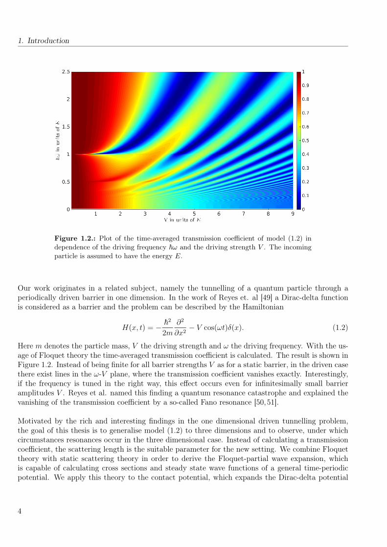
Figure 1.2.: Plot of the time-averaged transmission coefficient of model (1.2) independence of the driving frequency ~ω and the driving strength V . The incomingparticle is assumed to have the energy E.
Our work originates in a related subject, namely the tunnelling of a quantum particle through aperiodically driven barrier in one dimension. In the work of Reyes et. al [49] a Dirac-delta functionis considered as a barrier and the problem can be described by the Hamiltonian
H(x, t) = − ~2
2m
∂2
∂x2− V cos(ωt)δ(x). (1.2)
Here m denotes the particle mass, V the driving strength and ω the driving frequency. With the us-age of Floquet theory the time-averaged transmission coefficient is calculated. The result is shown inFigure 1.2. Instead of being finite for all barrier strengths V as for a static barrier, in the driven casethere exist lines in the ω-V plane, where the transmission coefficient vanishes exactly. Interestingly,if the frequency is tuned in the right way, this effect occurs even for infinitesimally small barrieramplitudes V . Reyes et al. named this finding a quantum resonance catastrophe and explained thevanishing of the transmission coefficient by a so-called Fano resonance [50,51].
Motivated by the rich and interesting findings in the one dimensional driven tunnelling problem,the goal of this thesis is to generalise model (1.2) to three dimensions and to observe, under whichcircumstances resonances occur in the three dimensional case. Instead of calculating a transmissioncoefficient, the scattering length is the suitable parameter for the new setting. We combine Floquettheory with static scattering theory in order to derive the Floquet-partial wave expansion, whichis capable of calculating cross sections and steady state wave functions of a general time-periodicpotential. We apply this theory to the contact potential, which expands the Dirac-delta potential
4

1.4. Outline of the Thesis
to three dimensions, and observe the emergence of scattering resonances. Those are manifested by adiverging scattering length instead of a vanishing transmission coefficient and allow us to control thescattering length and therefore the inter-particle interaction by time-periodic driving. We are ableto describe the shape of these resonances by a simple formula and determine position and width foralmost arbitrary driving frequencies.
A possible experimental realisation of our findings is a magnetic Feshbach resonance with a time-periodic magnetic field, which is applied in its vicinity [3]. This driven Feshbach resonance can beinduced in wide range of magnetic field strengths and the enhancement can be controlled by thedriving frequency. This allows a larger experimental flexibility, as the magnetic field can be set tovalues away from the actual resonance without loosing the enhancement of scattering. Additionally,our theory can be applied to systems, where a Feshbach resonance is not yet present. This wouldallow the tuning of the interaction strength in a case, where it is not be possible without periodicdriving.
1.4. Outline of the Thesis
This thesis combines the field of scattering physics and time-periodic forcing. While Chapters 2-4are reviewing relevant topics, Chapters 5-8 contain own work. As an introduction, we review inChapter 2 the scattering theory for a quantum particle in a time-independent potential, which isable of treating the two-body problem of interacting particles. We discuss how scattering quantitieslike the scattering amplitude and cross section are calculated using the partial wave expansion.
We apply in Chapter 3 the scattering theory in the context of Feshbach resonances. After a theoret-ical explanation for the emergence of Feshbach resonances, we survey both experimental realisationand theoretical prediction of those in the regime of ultracold quantum gases.
The focus of Chapter 4 lies on time-periodically driven systems. We introduce Floquet theory, whichis capable of solving the time-dependent Schrödinger equation exactly for arbitrarily large drivingstrengths and frequencies. A key feature of this method is, that it allows us to map the time-periodicSchrödinger equation to a static one in a larger Hilbert space and therefore to calculate steady states.
Using the prior Chapters as fundamentals, we derive in Chapter 5 the Floquet-scattering theory.It is capable of describing the scattering of a quantum particle by a time-periodic potential. We de-fine effective scattering quantities by time averaging and derive the Floquet-partial-wave expansionfor calculating these quantities. Similar to Chapter 4, the scattering by a time-periodic potentialcan be seen as the scattering by a static one in a more complicated Hilbert space. We finish thisChapter by investigating the low energy limit of Floquet scattering.
Chapter 6 applies Floquet-partial wave expansion to the contact interaction, which is able to de-scribe the interaction of ultracold atoms. We show for sinusoidal driving, that the equation describingscattering by the local contact interaction can be mapped to a recursion relation between Fourier
5

1. Introduction
coefficients of the steady state wave function and overview methods of solving it. Despite the recur-sion being non linear in the Fourier index, it can be solved exactly by numerical methods.
As a key result we discover in Chapter 7 a strong enhancement of scattering, named scatteringresonance, which is tunable by the periodic driving of the contact interaction. We explain thesescattering resonances by the extended Hilbert space of Floquet theory and show that they emergeif the scattered particle has the same energy as a driving induced bound state. Using this conditionwe determine the position of the scattering resonances. We then evaluate additional properties ofthe resonances by fitting simplified formulas to their shape and show that they fulfil the so calledanti-Kramers-Kronig relations. At last we investigate the case of small and large driving frequencies,where an analytic solution of the recursion is available.
In Chapter 8 we consider the more complicated case of a time-periodic potential, which is notdriven sinusoidally. In this case higher harmonics of the driving frequency occur. We show thatalso in this case scattering resonances show up and investigate the effect of the more general drivingscheme on these resonances.
Chapter 9 is devoted to the Conclusion and the Outlook.
6

2. Scattering Theory
Scattering theory is a powerful tool in order to understand and characterise the interaction of particlesand quantify its strength in easily interpretable quantities like the total cross section. As it is the basisof the following Chapters, a brief overview of the time-independent scattering theory of quantumparticles is given. In Section 2.1 we give an introduction in the considered setting, while in Section2.2 important quantities are introduced. Section 2.2.1 is focused on the partial wave expansion,while Section 2.2.2 discusses the case of low energy physics. As an example we show in Section 2.3the scattering by a hard-sphere potential.
2.1. Introduction
In this Section we consider the elastic scattering of a particle with mass m and no internal degreesof freedom by a static potential V (r). The problem can be described by the Hamiltonian
H = − ~2
2m∆ + V (r). (2.1)
In order to use the theory below, the potential is assumed to vanish faster than 1/r
limr→∞
V (r)r = 0, (2.2)
where by r the modulus of the position vector r is denoted. Elastic scattering of two distinguishableparticles with massesm1 andm2 can be mapped to the above setting by transforming to the center-ofmass system [52]. The motion of the center-of mass can be separated and only the kinetic energy ofthe relative motion appears in the Schrödinger equation. The Hamiltonian of relative motion can bemapped to (2.1) by setting the reduced mass µ = (m1m2)/(m1 +m2) equal tom and the inter-atomicpotential U(r2 − r1) equal to V (r) while introducing the particle seperation r = r2 − r1.
2.2. Asymptotic Form and Scattering Quantities
In order to gain insight over general features of scattering, we assume an incoming plane wavealong the z-axis and a potential centred at r = 0. Intuitively, the interaction causes emissionof the scattered wave function ψsc(r). It adds with the plane wave to the total wave-function
7

2. Scattering Theory
ψ(r) = eikr + ψsc(r). As it is the asymptotic solution of the Schrödinger equation (2.1) for largeradii [53], the scattered wave can be approximated by ψsc(r) ≈ f(k, θ, φ) e
ikr
r. It is a spherical wave
with an amplitude only depending on the wave-vector k, the polar angle θ and the azimuthal angleφ [54]. Therefore the asymptotic solution of the scattering problem for large r is given by
ψ(r) = eikr + f(k, θ, φ)eikr
r. (2.3)
The quantity f(k, θ, φ) is called scattering amplitude and is the basis for calculating the followingcross sections, which can be measured in experiment.
The differential cross section dσdΩ
is defined as the probability current flowing through an infinitesi-mal small area dA = r2dΩ located at the solid angle Ω = (θ, φ) divided by dΩ and the probabilitycurrent density of the incoming wave [53]
|jin|dσ
dΩdΩ = joutr
2dΩ. (2.4)
Here dΩ points in radial direction outside a sphere. By relating the probability current of theincoming wave jin = ~k
mto the one of the outgoing wave jout = ~k
mr2 |f(k, θ, φ)|2er + O(
1r3
)in the
limit of large radii, one gets an equation connecting the differential cross section to the scatteringamplitude
dσ
dΩ= |f(k, θ, φ)|2. (2.5)
The total cross section σ is defined as the integral of the differential one over the full solid angle
σ =
∫Ω
dΩdσ
dΩ. (2.6)
Both differential (2.5) and total cross section (2.6) are measurable quantities.
2.2.1. Partial Wave Expansion
In the case of a spherical symmetric potential, the partial wave expansion leads to an intuitive wayof rewriting and solving the scattering problem (2.1). A spherical symmetric potential implies avanishing commutator between the Hamiltonian and the angular momentum operator L = r × p
[H, L] = 0. (2.7)
Thus angular momentum l is a good quantum number and the solution of the Schrödinger equationcan be expressed in terms of the eigenstates of the angular-momentum operator, which are givenby the spherical harmonics Y m
l (θ, φ). As the scattering problem has cylindrical symmetry, onlythe spherical harmonics without φ-dependence and therefore the magnetic quantum number m = 0will contribute to the wave function. As the spherical harmonics with m = 0 are proportional toLegendre polynomials Pl(cos(θ)) [53], the wave function can be written in the form
ψ(r, θ, φ) =∞∑l=0
Rl(r)Pl(cos(θ)). (2.8)
8

2.2. Asymptotic Form and Scattering Quantities
By separating the radial and the angular degrees of freedom, the radial-Schrödinger equation forRl(r) can be derived (
∆r + k2 − veff(r))Rl(r) = 0. (2.9)
Here, ∆r = 1r2
∂∂rr2 ∂
∂ris the radial-Laplace operator and veff(r) = l(l+1)
r2 + 2m~2 V (r) the effective
potential including the centrifugal barrier l(l+1)r2 . In order to connect the cross section to the solution
of (2.9), only the behaviour of the wave function for large radii is important. In this case the effectivepotential in equation (2.9) can be neglected and (2.9) is solved by
Rl(r) = Ale−ikr
r+Bl
eikr
r, (2.10)
which consist of an incoming and outgoing spherical wave. As the total flux through a sphere aroundthe origin should be zero, both coefficients Al and Bl have the same absolute value. This conditionsimplifies the description of the scattering process, as it allows us to introduce the scattering phaseδl by setting [53]
Bl = e2iδlAl. (2.11)
The plane wave eikr can be expanded in Legendre polynomials [53]
eikr = eikr cos(θ) =∞∑l=0
(2l + 1)iljl(kr)Pl(cos(θ)). (2.12)
Here we introduced the spherical Bessel function jl(x) [53, 55, 56], whose limit of large argument isgiven by
jl(x) ≈sin(x− lπ
2)
x. (2.13)
Comparing (2.8) with (2.10) to (2.3), while expressing the occurring plane wave by (2.12) and (2.13),reveals the concrete value of the Al coefficients
Al = (−1)l(2l + 1)i
2k(2.14)
and the asymptotic Form of the wave function
Rl(r) ∝1
rsin(kr − lπ
2+ δl). (2.15)
The influence of the potential on the scattered-wave function is solely expressed by the value of thescattering phase, which leads to an additional shift of the wave function for large values of r. It isnegative for repulsive potentials and positive for attractive ones.
The scattering amplitude can be calculated by comparing the asymptotic waveform (2.3) using(2.12) with the limit of large radii of the ansatz (2.8) to
f(k, θ) =∞∑l=0
fl =∞∑l=0
2l + 1
keiδl sin(δl)Pl(cos(θ)). (2.16)
9

2. Scattering Theory
The total cross section evaluates to
σ =4π
k2
∞∑l=0
(2l + 1) sin2(δl) (2.17)
This equation shows, that all partial waves contribute to the total cross section and that it can becalculated by knowing all scattering phases. The contribution of the l = 0 part is called s-wavescattering, l = 1 p-wave scattering and so on. The value of the total cross section depends on theform of the scattering potential as well as the particle energy.
At last, we proof the optical theorem, which expresses the unitary of the scattering process. Itlinks the imaginary part of the scattering amplitude in forward direction θ = 0 to the total crosssection and can be derived by evaluating the formulas (2.16) and (2.17) using θ = 0 to
σ =4π
kIm f(θ = 0). (2.18)
An alternative, but more complicated, derivation [56, p. 26] reveals that it states, that the lossesof probability flux through the scattering process, being proportional to σ, are compensated by theinterference of incoming plane wave and scattered wave in forward direction. This interference isexpressed in equation (2.18) by Im f(θ = 0).
2.2.2. Scattering Length
In the low energy limit, where the wave vector k of the incoming particle goes to zero, the scatteringproperties can be characterised by a single parameter, which is independent of the detection angleθ and particle energy. For any potential growing like 1
rs, with s > 2l + 3, it can be shown [57, pp.
45], [58, p. 306] that
limk→0
k2l+1 cot(δl) = − 1
al, (2.19)
where al is the energy independent l-wave scattering parameter. Equation (2.19) shows that inthe low energy limit s-wave scattering is dominant, as all scattering phases corresponding to higherpartial waves are suppressed by a factor of k2l. We therefore can characterise the scattering processat low wave vectors by the s-wave scattering length
a = al=0, (2.20)
which does not depend on the energy or the angle θ. Therefore s-wave scattering at low energy ishas a simple structure in comparison to higher partial waves or finite energies. The scattering length(2.20) determines the total cross section to
σ = 4π|a|2. (2.21)
This equation gives an intuition for the scattering length, as it relates it to a length scale character-ising the cross sectional area.
10

2.3. Scattering by a Hard-Sphere Potential
By inserting equation (2.19) into (2.16) we find that the scattering length can be calculated byperforming the limit of vanishing momentum of the scattering amplitude
a = − limk→0
f(k, θ). (2.22)
At this point we note, that the scattering length is only the first contribution in the so-called effectiverange expansion [57, 58]. Equation (2.22) will be generalised in Chapter 5 to the case of scatteringby a time-periodic potential and is therefore fundamental to this thesis.
2.3. Scattering by a Hard-Sphere Potential
As it is the most simple and fundamental case of a scattering potential, we discuss the scattering bya hard-sphere potential. It consists of a sphere with infinite large repulsion around the origin
V (r) =
∞ , r < r0
0 , r > r0
. (2.23)
Outside the radius r0 equation (2.9) is solved by spherical Bessel jl(kr) and spherical Neumann yl(kr)functions [53, 55, 56]. These functions have the following asymptotic properties for large argumentsx
jl(x) ≈sin(x− lπ
2)
x, yl(x) ≈ −
cos(x− lπ2)
x(2.24)
and for small arguments
jl(x) ≈ xl
(2l + 1)!!, yl(x) ≈ (2l − 1)!!
xl+1. (2.25)
The double factorial n!! is defined by only multiplying the odd numbers up to the integer n. Thesolution outside the sphere can be written in the form
Rl(r) = Aljl(kr) +Blyl(kr). (2.26)
With the substitutionAl = Cl cos(δl), Bl = −Cl sin(δl) (2.27)
the asymptotic Form of (2.26) is expressed by the scattering phase δl, which can be computed bythe continuity condition at the radius r0 to be
tan(δl) =jl(kR0)
yl(kR0). (2.28)
Inserting the approximation (2.25) the result for small kr0 is derived to
δl ≈ −(kr0)2l+1
(2l + 1)!!(2l − 1)!!. (2.29)
11

2. Scattering Theory
This result again shows the dominance of the s-wave scattering in the low energy limit: If theparameter kr0 is small, higher angular momentum contributions drop off very fast and only thes-wave scattering phase with angular momentum l = 0 contributes to the scattering. The resultings-wave scattering length (2.20)
a = r0 (2.30)
equals the radius of r0 of the repulsive potential and in this case the scattering length can be relatedto the size of the scattering potential.
We now want to summarise this Section shortly. We gave an introduction into static scatteringtheory and discussed how the measurable scattering cross section can be calculated by the use ofquantum mechanics. We defined the s-wave scattering length (2.20), which characterises the scat-tering process in the case of low-energy physics. Due to its importance we will lay a main focuson investigating the scattering length in the further Chapters. As two-body collisions are a domi-nant process in interacting many-body systems, the scattering length characterises the interactionstrength of such systems at low temperatures [59]. One example are Bose-Einstein condensates,where the scattering length can be tuned by the usage of Feshbach resonances, which we will discussin the next Section in detail.
12

3. Feshbach Resonances
This Chapter is devoted to Feshbach resonances. In Section 3.1 we give an introduction into those,while in Section 3.2 we provide an overview over those resonances and summarise their realisationin ultracold gas experiments. In the last part of this Section we survey literature investigating howperiodic driving and ac-magnetic fields can be used in order to tune and induce resonances.
3.1. Introduction to Feshbach Resonances
A resonance can be understood as an almost bound state. As it is not truly bound it is associatedwith a lifetime [56] and is seen in scattering events in a phase shift of approximately π [38] of thescattering phase combined with an enhancement of the scattering amplitude. Resonances can bedivided into two groups: The shape resonances occur due to a quasi-bound state, whose energy liesin a continuum. One example is a trapped state behind a potential barrier, which can decay intothe continuum due to the finiteness of the barrier. As the properties of these resonances depend onthe shape of the potential, they are called shape resonances.
The second type of resonances are the Feshbach resonances, which appear in scatting of multi-channel systems [56]. Within a multi-channel system two scatterers with multiple internal statesinteract. Each of these internal states is labelled by a channel number or a quantum number ofthe internal degrees of freedom. An example of a multi-channel system are atoms in a constantmagnetic field, where energy levels split due to the Zeeman effect. The internal states of the atom,which can be labelled by the total angular momentum F of the atom and its projection along thespin-quantization axis mF [60], are the channels, if the atoms are viewed as a multi-channel system.If a channel supports a scattering state, it is said to be open, while closed channels support boundstates. In order to observe a Feshbach resonance, a system needs to have both open and closedchannels. The coupling between these channels can modify the scattering properties in the openchannels significantly, if the energy of the scattering state is close to the energy of a bound state ina closed channel. These resonances are named after Hermann Feshbach, as he developed a resonantscattering scheme in the field of nuclear physics in Refs. [61,62].
We will now discuss Feshbach resonances in more detail, following Refs. [38, 56, 63, 64] and assumea scatterer with multiple internal states possessing the energy Ei, which equal the threshold energyof the potential Vi(r) in channel i
limr→∞
Vi(r) = Ei. (3.1)
13

3. Feshbach Resonances
0 0.5 1 1.5 2
r in A.U.
-3
-2
-1
0
1
2
3E
nerg
y
Figure 3.1.: A sketch of the physics behind equations (3.4). The open channel(blue) supports a free solution with energy E, while the closed (red) possesses abound state with energy E0. If both energies approach each other, a Feshbachresonance occurs. The respective channel thresholds are included with dashed lines.
We now specialise to a two-channel system with an open and a closed channel. The first chan-nel is defined to be open and the channel thresholds are said to fulfil the relation E1 < E2. Weassume m to be the particle mass or the reduced mass if working in the centre-of mass frame. Thescattering state solution of the corresponding uncoupled Schrödinger equation in the first channel
[− ~2
2m
1
r2
∂
∂rr2 ∂
∂r+ V1(r)
]Run
1 (r) = E Run1 (r) (3.2)
is characterised by the background scattering length δBg. In order to have a free channel, the energyE must lie above E1. The second channel is considered as closed. It possesses in the uncoupled casethe bound state wave function R0(r) fulfilling the Schrödinger equation
[− ~2
2m
1
r2
∂
∂rr2 ∂
∂r+ V2(r)
]R0(r) = E0R0(r). (3.3)
As shown in Figure 3.1, the bound state energy E0 of the second channel is assumed to lie betweenE1 and E2. Introducing inter-channel coupling V12(r) the coupled radial Schrödinger equation for
14

3.2. Feshbach Resonances in Ultracold Quantum Gases
such a system can be written in the form[− ~2
2m
1
r2
∂
∂rr2 ∂
∂r+ V1(r)
]R1(r) + V12(r)R2(r) = E R1(r) (3.4)[
− ~2
2m
1
r2
∂
∂rr2 ∂
∂r+ V2(r)
]R2(r) + V12(r)R1(r) = E R2(r). (3.5)
If the coupling V12(r) between the channels is activated, the bound state u0(r) can lead to a resonance,as discussed in Ref. [56]. This resonance is seen in the scattering phase δ connected to the unboundwave function, as it splits into two parts
δ = δbg + δRes. (3.6)
The background phase δbg stems from scattering by the potential V1(r), while the resonant δRes
originates from coupling to the closed channel. Assuming a smooth energy dependence, this resonantphase can be approximated by [56]
tan(δRes) = − Γ/2
E − ER, (3.7)
where ER is the position of the resonance and Γ is its width. Both quantities can be expressedas matrix elements involving the channel coupling potential V12, the bound state and the regularsolution ureg
1 (r) together with the propagator G [56, p. 149] of the free channel. The position ERequals the energy of the bound state E0 plus an energy shift δE originating from the interactionwith the open channel
δE = 〈u0|V12GV12|u0〉. (3.8)
The width Γ is associated with a lifetime of the resonance and is calculated to be
Γ = 2π|〈u0|V12|ureg1 〉|2. (3.9)
Especially in the case of ultracold quantum gases the low energy limit of the scattering phasebecomes interesting. As shown in Section 2.2.2 the scattering length a is the relevant parameter andis given by [38]
a = − limk→0
δ
k= abg +
abgΓ0
−ER + iγ2
. (3.10)
Here k is the relative momentum and Γ0 = limk→0
Γ2kabg
is the low energy limit of the width Γ. Theimaginary part iγ/2 is added by hand in order to describe additional losses, which might occur, ifthe bound state has an additional decay channel.
3.2. Feshbach Resonances in Ultracold Quantum Gases
We overview the common methods to implement Feshbach resonances in ultracold quantum gasesand specialise in the end of the Section to the case of resonances induced by periodic driving. The
15

3. Feshbach Resonances
scattering length characterises the interaction of ultracold atoms [52, 59]. As Feshbach resonancesallow a tuning of the scattering length, they provide a powerful tool for tuning the inter-particleinteraction in an ultracold gas, which lead to the discovery of novel and interesting phenomena[38,44].
3.2.1. Magnetic Feshbach Resonance
Magnetic Feshbach resonances are a common tool in order to control the scattering length [38,63] byadjusting a spatially constant magnetic field. They have been first observed experimentally in a coldgas experiment with 23Na by Ref. [65] and with 85Rb by Ref. [66]. Atoms in a magnetic field obtaina splitting of their energy levels by ∆Ei = −µiB due to the Zeeman effect. As this shift dependson the magnetic moment µi of the particular internal state, changing of the magnetic field leads toa change of the relative energy between two channels. If this difference becomes zero, a Feshbachresonance occurs. Therefore the position of the resonance can be parametrised in the form [38], ifthe magnetic field is applied parallel to the difference of the magnetic moments
ER = δµ(B −B0). (3.11)
The variable B0 characterises the magnetic field at resonance position, δµ = µatoms − µpair is thedifference of magnetic moments between the two separated atoms in the open channel and the boundpair in the closed one. Losses through two body collisions described by γ in equation (3.10) canusually be neglected in the case of a magnetic Feshbach resonance [38]. With these assumptions thescattering length (3.10) simplifies to the well-known approximate formula [63]
a(B) = abg
(1− ∆
B −B0
). (3.12)
Here abg denotes the background scattering length, which is obtained away from resonance position.The width ∆ is given by
∆ = Γ0/δµ. (3.13)
Equation (3.12) is plotted in Figure 3.2. Close to the resonance the scattering length can be tunedto infinite repulsion or attraction. The width ∆ can be determined using Figure 3.2 (a). It is thedifference of the position of the resonance B0 and the magnetic field strength where the scatteringlength vanishes.
3.2.2. Optical Feshbach Resonance
An optical Feshbach resonance is created using laser light, which is nearly resonant to a transitionbetween a scattering state and an exited molecular bound state and therefore induces a coupling of
16

3.2. Feshbach Resonances in Ultracold Quantum Gases
-2 0 2
(B −B0)/∆
-5
0
5
a/a
bg ∆
(a) (b)
Figure 3.2.: (a): Plot of the approximative formula (3.12) of the scattering lengtha in case of a magnetically tuned Feshbach resonance without losses.(b): First experimental observation of a magnetic Feshbach resonance in a cold gasexperiment with 23Na. The Figure was created by Inouye et al. [65]
both [67–69]. The scattering length can be controlled by tuning the laser frequency ω or intensity Iinstead of a magnetic field [38] and follows the equation
a = abg
(1 +
Γ0(I)
~(ω − ω0 − δω(I)) + iγ/2
)(3.14)
But unlikely to most magnetic Feshbach resonances the bound state decays, which results in anon-vanishing loss parameter γ. Therefore the scattering length becomes complex, where real partcharacterises the scattering strength and the imaginary the particle loss [38, 70]. According toequation (3.14), the real part of the scattering length obtains a maximum at a finite value, restrictingthe tunability of the resonance. The behaviour of (3.14) is shown in Figure (3.3).
3.2.3. Microwave- and Radio Frequency induced Feshbach Resonances
These classes of resonances are induced or manipulated by the use of microwave (mw) and radiofrequency (rf) fields and have been discussed in recent literature [71–79]. The basic idea behind thoseconsiderations is coupling of different states by those fields. The coupling leads to an energy shiftof bound states in a field dressed picture and results in a Feshbach resonance, which is controllableby the fields. As in many setups an oscillating magnetic field is considered, the coupling strength islimited by the relatively weak magnetic dipole matrix elements. A pioneer in this topic was Moerdijk[71], who considered rf-fields for evaporative cooling but also suggested them for the creation ofresonances. Kaufmann et al. [72] investigated the coupling of bound states due to rf fields with astatic magnetic field close to a static Feshbach resonance in a experiment. Ref. [74] extended this tothe coupling of a colliding pair with a molecular bound state. Both predict the tuning of resonancesby changing both the frequency and strength of a rf field. Tscherbul et al. [75] discovered, that new
17

3. Feshbach Resonances
-3 -2 -1 0 1 2 3
-10
-5
0
5
Figure 3.3.: Plot of the real (blue) and imaginary part (red) of the scattering lengthin case of an optical Feshbach resonance for γ = 0.1Γ0. In contrast to a resonancewithout losses, an imaginary part exists around the central position and a finitemaximum of the real part occurs.
resonances can be induced by rf field using a coupled channel approach in a field dressed picture.Xie et al. [76] showed the ability of rf fields to tune the interspecies scattering length in 6Li + 40Kcollisions, while Owens et al. [78] obtained the creation of new resonances with 39K + 133Cs by usingscattering calculations in a field dressed basis.
3.2.4. Driving Induced Scattering Resonance
The driving induced scattering resonance will be the focus of this thesis and has been discussed inRefs. [3,4,80] in the case of a periodically driven magnetic Feshbach resonance. The underlying ideais to create a time-periodic inter-atomic potential by driving a parameter of the considered physicalsystem time periodically. As we pointed out in Chapter 1 and we will show in this thesis, a time-periodic potential is able to create bound states, which interact with scattering states in a way thatthey induce a resonance. A possible realisation of this resonance was suggested by Smith [3,80,81].He considered a magnetic Feshbach resonance with a time-periodic magnetic field [3]
B(t) = B1 +B2 cos(ωt), (3.15)
which is polarised along the spin-quantisation axis. He showed by using a Lippmann-Schwingerformalism that this results in a time-dependent potential inducing a Feshbach resonance at the biasmagnetic field B1, which does not need to coincide with the field strength where the static resonanceoccurs. By tuning the driving frequency ω and field strength B2 position and width of this artificiallycreated resonance can be tuned [80]. Smith named this method by "Modulated Magnetic FeshbachResonance".
18

3.2. Feshbach Resonances in Ultracold Quantum Gases
Here we go beyond his research and examine in Chapter 7 the driving induced scattering reso-nance in a more generalised setting and for a larger amount of driving strengths and give a deeperexplanation of their emergence. In order to do this, we extend in Chapter 5 scattering theory totime-periodic scattering potentials by using Floquet theory. This Floquet-scattering theory is capa-ble of solving Schrödinger equation in the case of a time-periodic Hamiltonians. As an introductionto this setting, we first discuss Floquet theory in the next Chapter.
19


4. Floquet Theory
In this Chapter Floquet theory is introduced. This theory can be used in order to solve timedependent, but periodic, problems exactly by converting them to a static problem in a more complexHilbert space. We initiate this Chapter in Section 4.1 by Floquet theorem, which can be consideredas the "The Bloch theorem in time". Section 4.2 introduces Floquet equation and summarisesrelevant properties of periodically driven systems. Section 4.3 is dedicated to the time evolution ofstates under a time-periodic Hamiltonian.
4.1. Floquet Theorem
Floquet theorem was initially stated in the context of ordinary differential equations [35] and can bewritten in terms of quantum mechanics in the following way [32, 33, 82]. A time-periodic Hamiltonoperator
H(t) = H(t+ T ), (4.1)
with ω = 2π/T as the driving frequency is considered. Then Floquet theorem states the existenceof solutions |ψ(t)〉 of the time dependent Schrödinger equation
i~∂
∂t|ψ(t)〉 = H(t)|ψ(t)〉, (4.2)
which are of the form|ψ(t)〉 = e−i
ε~ t|φ(t)〉. (4.3)
Here ε is called the quasi energy or the Floquet energy. It is not to be confused with the physicalenergy E, which is not necessarily a conserved quantity in a driven system. The Floquet mode |φ(t)〉has the same time-periodicity as the Hamiltonian (4.1)
|φ(t)〉 = |φ(t+ T )〉. (4.4)
Note that Floquet theorem is similar to Bloch theorem of solid-state physics [14,83]. Instead of havinga Hamilton operator being periodic in space, in Floquet theory the Hamiltonian is considered to betime periodic. The well-known quasimomentum can be mapped to the Floquet energy and the Blochfunction corresponds to the Floquet mode.
21

4. Floquet Theory
4.2. Floquet Equation and Properties of Floquet Modes
Using representation (4.3) of the wave function, an eigenvalue equation for the Floquet energy canbe derived by inserting (4.3) into (4.2):
H|φ(t)〉 = ε|φ(t)〉. (4.5)
This eigenvalue equation of the Floquet operator
H = H − i~ ∂∂t
(4.6)
is called the Floquet equation. It is defined on the Floquet-Hilbert space F = R⊗T , which consistsof the configuration space R of the original Hamiltonian H and the space of time-periodic functionsT . By using this Floquet-Hilbert space, time, which is regarded as a parameter in Schrödingerequation, is promoted to a coordinate. This extended Hilbert-space can be used to write down theFloquet equation in a way not using time explicitly. By using the Fourier transformation of bothFloquet mode and Hamiltonian
|φ(t)〉 =∞∑
n=−∞
e−inωt|φn〉, (4.7)
H(t) =∞∑
m=−∞
e−imωtHm, (4.8)
equation (4.5) can be mapped to a static one∞∑
m=−∞
Hm|φn−m〉 − n~ω|φn〉 = ε|φn〉, ∀n ∈ Z, (4.9)
which is involving the Fourier components |φn〉 of the Floquet mode. In addition this equation canbe written as an eigenvalue equation of an infinitely sized matrix
H =
. . . . . . . . .
. . . H1 H0 − (n− 1)~ω H−1 . . .
. . . H1 H0 − n~ω H−1 . . .
. . . H1 H0 − (n+ 1)~ω H−1 . . .. . . . . . . . .
. (4.10)
The eigenvalues of this matrix are given by the Floquet energies ε and the eigenvectors consist ofthe Fourier components of the Floquet modes
|φ〉 =
...|φn−1〉|φn〉|φn+1〉...
(4.11)
22

4.2. Floquet Equation and Properties of Floquet Modes
Figure 4.1.: A graphical representation of equation (4.9): The blue ovals representthe configuration space R labelled by Fourier indices n of the Floquet mode. Onthis Hilbert space the Hamiltonian H0 − ~nω acts in terms of a self energy. HigherFourier components of the Hamiltonian Hm lead to coupling of channels with dif-ferent Fourier index n. This coupling is indicated in the Figure by green and yellowarrows.
Equations (4.9) and (4.10) are a fundamental results of Floquet theory and visualised in Figure 4.1.Any time-periodic Schrödinger equation can be mapped to a static problem, which is located in alarger Hilbert space, by using Fourier transform. But the price of introducing a channel number bythe Fourier index n has to be paid, as equation (4.9) can be seen as a static multi-channel Schrödingerequation. This channel structure leads to a more complicated eigenvalue equation in comparison tothe static case, as the Floquet-Hilbert space is much larger than the static one, but equation (4.9) ismuch simpler to solve than the corresponding time-dependent Schrödinger equation. We introducethe concept of Floquet channels by locating the Fourier-component |φn〉 in the Floquet channel withnumber n.
From now on, we assume Floquet energy and modes to be labelled by a quantum number q andconsider a Floquet mode |φq〉 with corresponding Floquet energy εq. Then |φq,n〉 = einωt|φq〉 isalso a Floquet mode yielding the same physical wave function |ψ(t)〉, but it has a Floquet energyεqn = εq + ~nω. As the modes describe the same physical wave function, Floquet energies εq areunique only up to integer multiples of the driving frequency ~ω. Similar to the case in solid-statephysics, Brillouin zones can be introduced in frequency or Floquet-energy space, respectively. Dueto aforementioned ambiguity, the quasi energies εq can be mapped into the first Floquet-Brillouinzone, which is defined as the interval
[−~ω
2, ~ω
2
[and is used for the definition of the set
Q1.FBZ =
q : εq ∈
[−~ω
2,~ω2
[. (4.12)
23
4. Floquet Theory
The Floquet modes |φq,n〉 fulfil the orthonormality conditions of the scalar product of F :
〈〈φq,n|φp,m〉〉 =1
T
∫ T
0
dt〈φq,n(t)|φp,m(t)〉 = δq,pδn,m. (4.13)
Here 〈φq,n(t)|φp,m(t)〉 denotes the scalar product of R. If q and p are continuous indices, the firstKronecker delta has to be replaced by a Dirac-delta function. By using the Fourier transform of theFloquet mode (4.7) and the orthonormality relation, the completeness relation in F reads accordingto Ref. [82] ∑
q∈Q1.FBZ
∞∑n=−∞
|φq,n(t)〉〈φq,n(t′)| = IRδ(t− t′). (4.14)
We denote with IR the identity on the configuration space R. If the times t and t′ are equal up toan integer multiple of T , it is sufficient to sum over the first Brillouin zone in order to get a modifiedcompleteness relation ∑
q∈Q1.FBZ
|φq(t)〉〈φq(t)| = IR. (4.15)
As the last point of this Chapter, a general formula for time-averaged expectation values is given.We consider a time-dependent operator A(t):
A(t) =∞∑
n=−∞
e−inωtAn, (4.16)
which has the same time periodicity as the Hamilton operator. The time averaged expectation valueis then defined as
〈〈A(t)〉〉 = 〈〈ψ(t)|A(t)|ψ(t)〉〉 =1
T
∫ T
0
dt〈ψ(t)|A(t)|ψ(t)〉. (4.17)
If the wave function |ψ(t)〉 is assumed to be a Floquet state according to (4.4), the Fourier decom-position (4.7) can be used in order to write the expectation value in the form
〈〈A(t)〉〉 =∞∑
n,s=−∞
〈φn+s|As|φn〉. (4.18)
By setting A(t) = IR, this equation can be used in order to calculate the norm of the Floquet state|ψ(t)〉.
4.3. Time Evolution and Effective Hamiltonian
With the knowledge of the Floquet energies and the corresponding modes any quantum state |ψ(0)〉can be propagated by the Hamiltonian H(t). Let the propagator corresponding to H(t) with initialtime t0 = 0 be denoted by U(t, 0). The time dependence
|ψ(t)〉 = U(t, 0)|ψ(0)〉 (4.19)
24

4.3. Time Evolution and Effective Hamiltonian
of an arbitrary quantum state |ψ〉 can be explicitly calculated by inserting the identity (4.15) attime t = 0 into (4.19). Using the notation
cq = 〈φq(0)|ψ(0)〉, (4.20)
the propagated state can be written in the form |ψ(t)〉 =∑
q∈Q1.FBZU(t, 0)|φq(0)〉cq. Floquet theorem
validates that Floquet modes |φq(t = 0)〉 equal their corresponding steady state wave function|ψq(t = 0)〉 at t = 0 and therefore the time evolution of the Floquet mode |φq(0)〉 is given byU(t, 0)|φq(0)〉 = e−iεq/~ t|φq(t)〉. With this knowledge the time-evolved quantum state is written inthe form
|ψ(t)〉 =∑
q∈Q1.FBZ
cqe−i εq~ t|φq(t)〉. (4.21)
As we assumed |ψ〉 to be arbitrary, the propagator reads
U(t, 0) =∑
q∈Q1.FBZ
|φq(t)〉〈φq(0)|e−iεq/~ t. (4.22)
By again inserting identity (4.15) at t = 0, equation (4.22) can be rewritten as
U(t, 0) = Upe−iHeff/~ t, (4.23)
where Up =∑
q∈1.BZ|φq(t)〉〈φq(0)| is denoted as micromotion operator [31], as it deals with the time-
periodic part of the dynamics. The effective Hamiltonian
Heff =∑
q∈Q1.FBZ
εq|φq(0)〉〈φq(0)| (4.24)
contains the slowly varying components of the dynamics and all information about the Floquetenergies and the Floquet modes at times t = 0. As Up(t + T ) = Up(t) and Up(0) = I, the effectiveHamiltonian contains all information to propagate any quantum state at multiple integers of thedriving period T . The propagator has in this special case a simple structure of
U(nT ) = e−iHeff/~ nT = [U(T )]n, n ∈ Z. (4.25)
It is now the point to do some concluding remarks. In this Chapter we introduced Floquet the-ory, with which one is able to solve the time-dependent Schrödinger equation in the case of atime-periodic Hamiltonian. As a main point we saw by using Floquet theorem in combination withFourier transform, that we can map the time-dependent Schrödinger equation to a static one, whichis located in a more complex Hilbert space. We saw that this Floquet equation looks similar to amulti-channel Schrödinger equation. This fact we exploit in the next Chapter in order to generalisethe scattering theory of Chapter 2 to time-periodic potentials.
25


5. Floquet-Scattering Theory
In this Section we present a scattering theory for time-periodic potentials by usage of Floquettheorem. Due to the driving-induced channel structure, Floquet-scattering theory has similarities tomulti-channel quantum scattering theory [56], if the Fourier index n is viewed as a channel. Insteadof introducing a Lippmann-Schwinger formalism like Refs. [3, 80] our focus lies on the partial waveexpansion. We start in Section 5.1 with introducing time averaged scattering quantities. Withthis basic framework, the Floquet-partial wave expansion is presented in Section 5.2. We finishthis Section by the Floquet-optical theorem, which expresses the unitary of the Floquet-scatteringprocess. Section 5.3 is dedicated to the scattering of indistinguishable particles.
5.1. Coupled-Channel Equations and Cross Sections
In this Section we rewrite the time dependent scattering problem in a set of static coupled equations.This step is useful in order to introduce the scattering amplitude and cross section in an intuitiveway.
5.1.1. Coupled-Channel Equations
In order to investigate the effect of periodic driving on the scattering of quantum particles, we usea Schrödinger theory with a Hamiltonian
H = − ~2
2m∆ + V (r, t), (5.1)
where a time-periodic potential V (r, t) is considered. The period of the potential is denoted by T ,i.e.
V (r, t+ T ) = V (r, t), ∀t ∈ R. (5.2)
As presented in Chapter 4, the driving frequency ω is defined as ω = 2π/T . The Hamiltonian (5.1)can be interpreted in two ways. On the one hand it describes a single particle with mass m underthe influence of an external potential V (r, t). On the other hand it can be also used to describethe scattering of two particles with masses m1 and m2 by the inter-particle interaction U(r1 − r2, t)in the centre-of-mass system [55]. In this case the mass m has to be identified with the reduced
27

5. Floquet-Scattering Theory
mass µ = m1m2/(m1+m2) and the potential V (r, t) by the inter-particle interaction potential U(r, t).
In order to find a reasonable description of time-periodic scattering, the goal is to obtain the scat-tering behaviour of steady-state solutions ψ(r, t) = e−iε/~ tφ(r, t) of the Floquet-equation[
− ~2
2m∆ + V (r, t)− i~ ∂
∂t
]φ(r, t) = ε φ(r, t). (5.3)
The first step is to remove the explicit time dependence of the Floquet equation by using the Fouriertransform of the Floquet mode and the potential
φ(r, t) =∞∑
n=−∞
e−inωtφn(r) (5.4)
V (r, t) =∞∑
n=−∞
e−inωtVn(r) (5.5)
and to introduce the Floquet channel number by the Fourier-index n. Similar to (4.9), equation(5.3) can be written down in the form
− ~2
2m∆φn(r) +
∞∑m=−∞
Vm(r)φn−m(r) = (e+ n~ω)φn(r), ∀n ∈ Z. (5.6)
In this equation the coupling of Floquet channels is given by the Fourier-components of the potentialVn(r) which have n 6= 0.
5.1.2. Asymptotic Waveform
In order to derive the asymptotic behaviour of the Floquet mode and the form of the cross section,we first summarise necessary assumptions.
At first, we assume the potential V (r, t) to vanish faster than 1/r for large r
limr→∞
rV (r, t) = 0, ∀t ∈ R, (5.7)
where r is the modulus of the position vector r. Although this condition excludes Coulomb-like po-tentials, it is necessary for obtaining a simple expression of the asymptotic form of the Floquet modeand covers the in our thesis relevant case of scattering by inter-atomic and short range potentials.
Secondly, a plane wave is considered as an incoming wave function
ψin(r) = eikr. (5.8)
The wave vector k, considered to be parallel to the z-axis, is related to the energy of the plane waveby the dispersion relation for non-relativistic particles
E =~2
2mk2. (5.9)
28

5.1. Coupled-Channel Equations and Cross Sections
We assume the incoming wave to be located in the zeroth Floquet channel
φin(r, t) = δn,0eikr. (5.10)
By comparing the time-evolution of (5.8) and (4.3), we conclude that the energy of the incomingparticle equals the Floquet energy
E = ε. (5.11)
With this consideration we make an ansatz of the asymptotic wave function solving (5.6) in thecase of large r. This ansatz reads
φn(r) = δn,0eikr + fn
eiknr
r. (5.12)
In this equation the wave vector kn and the scattering amplitude fn in the n-th Floquet channel isintroduced. The Floquet scattering amplitude fn depends on the potential, on the driving frequency,on the Floquet energy ε and on the solid angle Ω = (θ, φ) of the scattered wave
fn = fn(Vn, ω, ε, θ, φ). (5.13)
In order to verify the ansatz, we show, that it solves (5.6). The Laplacian of fn(ε,Ω) eikr
revaluates
for the case of large radii to
∆fn(ε,Ω)eiknr
r= fn(ε,Ω)
1
r2
∂
∂rr2 ∂
∂r
(eiknr
r
)+eiknr
r3
∂
∂Ωfn(ε,Ω) (5.14)
= −k2nfn(ε,Ω)
eiknr
r+O
(1
r3
)In the next step we assume for simplicity a potential of the form Vm(r) = 1/r1+α and calculate
Vm(r)φn(r) = eikr/r1+α + eikr/r2+α = O(
1
r1+α
). (5.15)
Condition (5.7) ensures that α > 0 and that the influence of the potential on the asymptotic waveformcan thus be neglected as r goes to infinity. With those approximations the asymptotic waveform is(5.12) inserted into the coupled-channel equation (5.6)(
~2
2mk2n − n~ω
)(δn,0e
ikr +eikr
r
)= ε
(δn,0e
ikr +eikr
r
)+O
(1
r3
), (5.16)
in order to yield the dispersion relation defining the values of kn
~2
2mk2n = ε+ n~ω. (5.17)
If one works in the centre of mass system, the mass m in equation (5.17) has to be replaced by thereduced mass µ. Due to equation (5.11) we identify k0 with k. If the right-hand side of 5.17 becomesnegative, we get an imaginary kn = iκn. The asymptotic solution in this Floquet channel is not aspherical wave, but an exponentially decaying solution fne−κnr/r.
29

5. Floquet-Scattering Theory
5.1.3. Cross Section
The goal of this Section is to derive an expression for the time averaged differential and total crosssection. The starting point is a general definition of the differential cross section in a time dependentmanner similar to (2.4)
|jin|dσ
dΩ(Ω, t)|dΩ| = jscatt(Ω, t)r
2dΩ, (5.18)
but we assume an explicit time dependency. For a steady state solution (4.3) the probability currentreads
j(r, t) =~
2im
∞∑m,n=−∞
(φm(r)∗∇φn(r)e−i(n−m)ωt − φm(r)∇φn(r)∗e−i(m−n)ωt
). (5.19)
For the incoming plane wave, this evaluates to
jin =~k
m. (5.20)
In order to determine the probability current of scattered particles, the asymptotic waveform of thescattered wave fn(ε,Ω)eiknr/r is inserted into expression (5.19). The gradient is evaluated for larger to be
∇fn(ε,Ω)eiknr
r= fn(ε,Ω)
(ikn
eiknr
r− eiknr
r2
)er +
eiknr
r2
∂fn(ε,Ω)
∂ΘeΘ (5.21)
+eiknr
r2 sin(Θ)
∂fn(ε,Ω)
∂φeφ = iknfn(ε,Ω)
eiknr
rer +O
(1
r2
).
Inserting this into (5.19), the time-dependent differential cross section is evaluated. As we areinterested in the asymptotic behaviour of the wave function, we neglect terms of order 1/r2 orhigher
dσ
dΩ(ε,Ω, t) =
1
k
∞∑m,n=−∞
Im(iknf
∗m(ε,Ω)fn(ε,Ω)ei(kn−k
∗m)re−i(n−m)ωt
). (5.22)
This is the most general expression of the differential cross section. In the case of an imaginary wavevector, the corresponding summands ei(kn−k∗m)r decay exponentially and do not contributing to thecurrent for large r. In equation (5.22) different summands oscillate with different frequencies in timeand wave-vectors in space, as they are created by superposition of different Fourier components of theasymptotic Floquet state. This complicated behaviour is due to the time-dependency of the potentialand not monitored in static scattering theory. In the following we assume the driving frequency ω tobe large in comparison to the measuring process or the measuring process to be done such often atrandom times, that it is useful to only consider time averaged quantities 〈〈A〉〉 = 1
T
∫ T0dtA(t). This
simplifies the situation dramatically. The time averaged differential cross section is evaluated whileusing 1
T
∫ T0dt ei(n−m)ωt = δn,m to be
〈〈 dσdΩ〉〉 =
∞∑n≥nc
|fn(ε,Ω)|2knk, (5.23)
30
5.1. Coupled-Channel Equations and Cross Sections
where the critical index nc is defined by the formula
nc =⌈− εω
⌉, (5.24)
which includes the ceiling function d•e. This ensures that all kn with n ≥ nc are real, while all knwith n < nc are purely imaginary, such that the sum (5.23) only covers open Floquet channels. Asboth Floquet energy and driving frequency are positive, definition (5.24) ensures that the criticalindex is always smaller or equal than zero. In comparison to equation (2.5) of static single-channelscattering theory a sum over the squared modulus of the scattering amplitude fn of all free channels,weighted by kn/k, occurs.
A measure of the complete amount of scattered particles is the total cross section σ. It is theintegral of the differential cross section over all solid angles
σ =
∫dΩ
dσ
dΩ. (5.25)
Using the form of the differential cross section (5.23) the time averaged total cross section can bewritten in the form
〈〈σ〉〉 =∞∑
n≥nc
〈〈σn〉〉, (5.26)
where we have introduced the cross section in in Floquet channel n by
〈〈σn〉〉 =
∫dΩ|fn(ε,Ω)|2kn
k. (5.27)
As the incoming particle is located in the zeroth Floquet channel, no driving-field quanta andtherefore energy is added or subtracted, if the particle stays in it and scattering is elastic. Thereforethe cross section in Floquet channel zero is considered as the elastic cross section [4]
σel = 〈〈σ0〉〉, (5.28)
while the cross Section in channel n is related to inelastic scattering involving n quanta of the drivingfield. The total inelastic cross section calculates to
σin =∞∑
n≥ncn 6=0
〈〈σn〉〉. (5.29)
The scattering amplitudes fn(ε,Ω) can be used in order to define a time-dependent scattering am-plitude
f(t, ε,Ω) =∞∑
n≥nc
e−inωtfn(ε,Ω), (5.30)
and its time-average equals the scattering amplitude in zeroth Floquet channel
〈〈f〉〉 = f0. (5.31)
31

5. Floquet-Scattering Theory
In Chapter 7 we will used this quantity in order to observe the enhancement of scattering.
At last we point out the similarities of the coupled-channel picture of Floquet scattering to staticmulti-channel scattering theory, which is explained for example in Ref. [56, Chapter 3]. In multi-channel scattering theory an equation similar to (5.6) exists, and the shape of the asymptotic wave-forms equal each other if the channels of the multi-channel theory are identified with the Floquetchannels. Although multi-channel theory does not include time dependent quantities like in (5.22),the formula for the time-averaged differential cross section (5.23) is similar to the one obtained instatic multi-channel scattering theory.
5.2. Floquet-Partial Wave Expansion
Here we generalise the concept of the partial wave expansion to the case of time-periodic scattering.We specialise to spherical symmetric potentials.
5.2.1. Radial-Floquet Equation
Consider a spherical symmetric Hamiltonian H(r, t), which commutes with the angular momentumoperator L at all times
[H(r, t),L] = 0 ∀t ∈ R. (5.32)
This implies that L commutes with all Fourier components (4.8) of the Hamiltonian
[Hn(r),L] = 0,∀n ∈ Z. (5.33)
Using the rules for commutators [84] this result is used in order to prove that the commutator of Land the Floquet Hamiltonian (4.10) vanishes
[H,L]R⊗T = 0. (5.34)
With this knowledge the eigenfunctions of the angular momentum operator L can be included inthe eigenbasis of H. The eigenfunctions of L are given by the spherical harmonics Y m
l (Θ, φ). Theyare parametrised by the quantum number of orbital angular momentum l and its projection m onthe quantisation axis.
With this knowledge the Floquet modes and its Fourier components φl,n(r) can be decomposedin a radial and angular part
φl,n(r) = Rl,n(r)Pl(cos(θ)), (5.35)
where Pl(z) denotes the l-th Legendre polynomial. They appear instead of spherical harmonics,as we assume the incoming plane wave to be directed along the z-axis. In this case the problemis rotational symmetric and therefore the φ dependence of the spherical harmonics drops out like
32

5.2. Floquet-Partial Wave Expansion
in static scattering theory. By introducing equation (5.35) time dependency is fully put into theradial part of the wave function. After inserting these coefficient functions in the coupled-channelequations (5.6) and separating the angular motion using ∆ = ∆r − L2
~2r2 , equation
− ~2
2m∆rRl,n(r) +
~2l(l + 1)
2mr2Rl,n(r) +
∞∑m=−∞
Vm(r)Rl,n−m(r) = (ε+ n~ω)Rl,n(r) (5.36)
is derived as an intermediate step. We denoted with ∆r = 1r2
∂∂rr2 ∂
∂rthe radial part of the Laplacian.
Like in the time-independent partial wave expansion, a centrifugal barrier including the angularmomentum quantum number l adds to the radial motion. Scaling by −2m
~2 , introducing ~2
2mk2n =
ε+ n~ω and vm(r) = 2m~2 Vm(r) leads to the radial Floquet equation[∆r + k2
n −l(l + 1)
r2− v0(r)
]Rl,n(r) =
∑m6=0
vm(r)Rl,n−m(r). (5.37)
This equation is central to this thesis, as its solution gives access to all scattering quantities of a givenpotential. For vanishing right-hand side the special case of time-independent scattering is recovered.In general, the explicitly time-dependent part leads to a coupling of the different Floquet channels.A schematic view on this is given by Figure 5.1. The Fourier components v±1 lead to a couplingof nearest neighbour channels, while v±2 couples next-nearest neighbours. Although only in thezeroth Floquet channel an incoming wave is present, scattered waves can occur in all free channelsdue to the periodic driving, where channels supporting imaginary wave vectors posses exponentiallydecaying wave functions. This structure is similar to static scattering theory but the fact that inFloquet-scattering infinitely many Floquet channels are present [4].
5.2.2. Scattering Amplitudes in Floquet-Partial Wave Expansion
The aim of this Chapter is to derive a closed formula for the scattering amplitudes fn in the sense ofa partial wave expansion, which is presented in Section 2.2.1 in the case of static scattering theory.The beginning of this consideration is the limit of large r of the radial Floquet equation (5.37),where the potential vm(r) can be neglected, but we do not neglect the centrifugal term. In this caseequation (5.37) gets decoupled (
∆r + k2n −
l(l + 1)
r2
)Rl,n(r) = 0. (5.38)
This equation can be solved by spherical Hankel functions h±l (knr) [85], which are defined by
h±l (x) = ∓i(−x)l(
1
x
∂
∂x
)le±ix
x, (5.39)
and are related to spherical Bessel jl(x) and Neumann yl(x) [53, 55] functions by
h±l (x) = jl(x)± iyl(x). (5.40)
33

5. Floquet-Scattering Theory
Figure 5.1.: Visualisation of a Floquet-Scattering Process. An incoming wave φino
is considered in the zeroth Floquet channel. Scattering by the time independentpart V0 (indicated by blue circles) of the potential leads to elastic scattering, wherethe outgoing wave φout
0 stays in the same channel. The first Fourier componentV1 (drawn in green) leads to a coupling of neighbouring Floquet channels, whilesecond component V2 (drawn in orange) couples next-nearest neighbours. Due tothis coupling the particle can be scattered inelastic to higher Floquet channels orbecome a bound state located in the channels with negative index n. The processeswith V1 involve one quantum of the drive field, while the ones with V2 involve two.The propagating waves are shown by a wave-package, while the bound states aredisplayed by an exponentially damped wave function.
The first two spherical Hankel functions are
h+0 (x) = −ie
ix
x, h−0 (x) = i
e−ix
x, (5.41)
h+1 (x) =
(1
x+
i
x2
)eix, h−1 (x) =
(1
x− i
x2
)e−ix. (5.42)
Similar to (2.24), in the limit of large arguments these functions read
h±l (x) = ∓e±(x−π
2l)
x. (5.43)
34
5.2. Floquet-Partial Wave Expansion
As it is seen from its shape, the spherical Hankel functions with a plus index correspond to incomingwaves and the ones with a minus index to outgoing.
The limit of the wave function for large radii is sufficient in order to investigate scattering proper-ties. Therefore we choose as an ansatz for the asymptotic radial wave function a superposition ofthe asymptotic limit of the spherical Hankel functions
Rl,n(r) = Al,nie−i(knr−
π2l)
knr−Bl,ni
ei(knr−π2l)
knr. (5.44)
If we insert (5.44) into
φn(r) =∞∑l=0
Rl,n(r)Pl(cos(θ)), (5.45)
we get the asymptotic form of the wave function. In order to be consistent, this should equal equation(5.12)
δn,0eikr + fn(ε, θ)
eiknr
r=∞∑l=0
[Al,ni
e−i(knr−π2l)
knr−Bl,ni
ei(knr−π2l)
knr
]Pl(cos(θ)). (5.46)
By expanding the plane wave in a sum of angular momenta as in equation (2.12)
eikr =∞∑l=0
(2l + 1)iljl(kr)Pl(cos(θ)) =∞∑l=0
2l + 1
2il[h+
l (kr) + h−l (kr)]Pl(cos(θ)) (5.47)
and expressing jl(x) via (5.40) and (5.43) by the asymptotic limit of h±l (x), this equation can berewritten in the form
fn(ε, θ)eiknr
r=∞∑l=0
(Bl,n −
2l + 1
2ilδn,0
)−ieiknr(−i)l
knrPl(cos(θ))
+
(Al,n −
2l + 1
2ilδn,0
)ie−iknril
knrPl(cos(θ))
(5.48)
Since the scattered wave only contains outgoing waves, the term in front of the e−iknr factor has tovanish. This sets the coefficients Al,n to be
Al,n =2l + 1
2ilδn,0. (5.49)
Thus, the scattering amplitude fn(ε, θ) is determined by the coefficients Bl,n to be
fn(ε, θ) =1
kn
∞∑l=0
(−i)l+1
[Bl,n −
2l + 1
2ilδn,0
]Pl(cos(θ)) (5.50)
Note that the scattering amplitude can be written as a double sum of fl,n(ε, θ) while using
fl,n(ε, θ) = (−i)l+1[Bl,n −2l + 1
2ilδn,0]Pl(cos(θ). (5.51)
35

5. Floquet-Scattering Theory
By inserting (5.50) into (5.23) the time-averaged differential cross section is calculated by the knowl-edge of the Bl,n
〈〈 dσdΩ〉〉 =
∞∑n≥nc
1
knk
∞∑l,l′=0
[B∗l,n −
2l + 1
2(−i)lδn,0
] [Bl′,n −
2l′ + 1
2il′δn,0
]Pl(cos(θ))Pl′(cos(θ)) (5.52)
The integration over the angle θ by using the orthogonality relation of the Legendre polynomials∫ 1
−1dzPl(z)Pl′(z) = δl,l′
22l+1
leads to an expression for the time-averaged total cross section
〈〈σ〉〉 =∞∑
n≥nc
∞∑l=0
4π
knk
∣∣∣∣Bl,n −2l + 1
2ilδn,0
∣∣∣∣2 1
2l + 1. (5.53)
This is similar to expression (2.17) of static scattering theory, but in contrast to (5.53), the scatteringphase has been introduced in equation (2.11). We now generalise the concept of the scattering phaseδl,n to Floquet-scattering theory by defining
Bl,n =2l + 1
2ile2iδl,n . (5.54)
In contrast to the definition in Chapter 2 it is allowed to be complex
δl,n = βl,n + iγl,n. (5.55)
The real part βl,n of the phase describes a phase shift of the wave function due to the scatteringprocess, while the imaginary part γl,n describes gains and losses due to scattering into and fromdifferent Floquet channels. Using the scattering phase according to (5.54) the scattering amplitudecan be expressed in the familiar form
f0(ε, θ) =1
k
∞∑l=0
(2l + 1)eiδl,n sin(δl,n)Pl(cos(θ)), (5.56)
fn(ε, θ) =1
kn
∞∑l=0
2l + 1
2ie2iδl,nPl(cos(θ)), n 6= 0. (5.57)
Correspondingly the total cross section reads
〈〈σ〉〉 =∞∑l=0
4π
k2(2l + 1)e−2γl,0| sin(δl,0)|2 +
∞∑n≥ncn6=0
4π
knk(2l + 1)
e−4γl,n
4
. (5.58)
This formula shows in an intuitive way the respective contribution of different channels to the Flo-quet scattering. The channel with the incoming wave n = 0 contributes to scattering both by phaseshift and losses as displayed in the first summand of equation (5.57), while the other channels onlycontribute through their gain and loss factor γl,n.
36

5.2. Floquet-Partial Wave Expansion
Similar to equation (2.22) in static scattering theory we define the Floquet-scattering length aFl(t)as the negative limit of vanishing energy of the Floquet-scattering amplitude
− limk0→0
fn(ε, θ) = aFln , (5.59)
where aFln are the Fourier-coefficients of aFl(t). The time averaged scattering length is defined as
ascatt = 〈〈aFl(t)〉〉 = aFl0 . (5.60)
This definition is central to this thesis, as it allows us to characterise the scattering by a time-dependent potential at low energies by a single parameter. Similar to static scattering theory,s-wave scattering is dominant at low energies in the driven case [4,80] and because of the additionalconservation of angular momentum s-wave scattering is present in all Floquet channels. As s-wavesare radial symmetric, the scattering length (5.59) has no dependence on the angle θ.
5.2.3. Floquet-Optical Theorem
In this section we will derive and discuss the Floquet-optical theorem, which will be of great use inChapter 7. Starting point of its derivation by Floquet-partial wave expansion is to note, that thetime-averaged probability current can be separated in partial wave currents 〈〈j〉〉l by
〈〈j〉〉 =∞∑l=0
〈〈j〉〉l. (5.61)
Inserting the wave function (5.45), while using as radial part the asymptotic form (5.44), and eval-uating the Legendre polynomials at forward direction θ = 0, the large r-asymptotic of the timeaverage of the l-wave current is derived to be
〈〈j〉〉l =~mr2
∞∑n≥nc
1
kn
(|Bl,n|2 − |Al,n|2
)er +O
(1
r3
)(5.62)
As in Schrödinger theory no probability is created or destroyed during a scattering process and thedifferent l-wave solutions are decoupled, the integral of each l-wave current over a sphere of radiusr0 vanishes ∫
dΩr2er〈〈j〉〉l = 0. (5.63)
The surface integral of 〈〈j〉〉l evaluates to
∞∑n≥nc
4π
kn
(|Bl,n|2 − |Al,n|2
)= 0. (5.64)
This equation describes the unitary of the scattering process, because it was derived from the van-ishing of the probability flux through a surface around the origin. This statement can be refined
37

5. Floquet-Scattering Theory
further by completing the square |Bl,n|2 − |Al,n|2 = |Bl,n − Al,n|2 + 2Re (Bl,nA∗l,n) − 2|Al,n|2 and
inserting (5.49) for Al,n to∞∑
n≥nc
4π
kn|Bl,n −
2l + 1
2ilδn,0|2 = −4π(2l + 1)
(Re [Bl,0(−i)l]− 2l + 1
2
). (5.65)
While multiplying by 1k0(2l+1)
and doing the l-summation, the left-hand side of equation (5.65) isexactly the time-averaged total cross section (5.53), while the right-hand side is proportional to theimaginary part of the Floquet-scattering amplitude (5.50). This yields the Floquet-optical theorem
〈〈σ〉〉 =4π
k0
Im f0(ε, θ = 0). (5.66)
It is very fundamental, as it connects the total cross section to the imaginary part of the scattingamplitude in the zeroth Floquet channel and ensures, like in the static case, the unitary of theFloquet-scattering process. Similar to the static case, the part with Im f0 originates from an in-terference term of incoming plane wave and outgoing special wave 2Re (Bl,nA
∗l,n) − 2|Al,n|2, while
〈〈σ〉〉 comes due to the probability current of the scattered wave. This implies, that Floquet-opticaltheorem does the statement, that losses of probability flux due to the scattered wave are compen-sated by the interference of plane and scattered wave in forward direction. Note, that only thescattered wave in the zeroth channel, in which also the incoming plane wave is located, contributesto this interference, while the cross section 〈〈σ〉〉 has a contribution of all Floquet channels. Sincethe probability current (5.61) separates in l-wave currents, Floquet optical theorem can be restatedin the case, where 〈〈σ〉〉 and f0 only cover contributions form l-wave scattering. In the case of s-wavescattering all scattering amplitudes are independent from the angle θ and the total cross section canbe directly calculated by multiplying (5.23) with 4π. The Floquet-optical theorem (5.66) can berestated as [4]
Im f0(ε) =∞∑
n≥nc
|fn(ε)|2kn. (5.67)
If the zero energy limit of (5.67) is done under the assumption, that all Floquet-scattering amplitudesare not single valued in this limit, we arrive at equation
Im aFl0 = −
∑n≥ncn6=0
|aFln |2kn. (5.68)
This equation states that the imaginary part of the time-averaged Floquet scattering length aFl0
at zero energy is related to the scattering of particles in higher channels, resulting in losses in thezeroth one. This means that the presence of inelastic scattering can be measured by a non-vanishingimaginary part of the Floquet scattering length in zeroth channel.
5.3. Indistinguishable Particles
In this Section the Floquet-scattering properties of indistinguishable particles are discussed. In thecentre-of mass frame, two identical particles are positioned at position r and −r, so the (anti)-
38

5.3. Indistinguishable Particles
symmetrised form of a scattering-wave function (5.12) reads
ψ±(r, θ, φ, t) =1√2e−iε/~t
eikr ± e−ikr +
∞∑n=−∞
[fn(ε, θ, φ)± fn(ε, π − θ, φ+ π)]eiknr
re−inωt
.
(5.69)The plus sign used for the case of bosons, while the minus sign gives the case of scalar fermions.As we only deal with scalar fields, both particles have to be spinless or spin polarised. We followthe common definition [52, 56, 86] of normalizing the scattering amplitude by only considering thecurrent in positive k direction as incoming
f±n (ε, θ, φ) = [fn(ε, θ, φ)± fn(ε, π − θ, φ+ π)] . (5.70)
This scattering amplitude leads a time-averaged differential cross section of
〈〈 dσdΩ〉〉± =
1
2
∞∑n≥nc
|fn(ε, θ, φ)± fn(ε, π − θ, φ+ π)|2knk, (5.71)
where the factor of 1/2 comes due to normalisation issues [56], with that the time-averaged totalcross section 〈〈σ〉〉± can be defined as the integral over the full solid angel of (5.71).
In the case of low energy physics we get as the s-wave scattering length a±scatt
a+scatt = 2ascatt (5.72)
for bosons anda−scatt = 0 (5.73)
for fermions.
We now arrived the end of this Section and we do a short summary of the most important findings.We treated the general form of scattering by a time-periodic potential and observed, that with theusage of Floquet theory the time-dependent scattering problem can be mapped to a static multi-channel problem with infinitely many channels. We were able to extend partial-wave expansion toscattering by time-periodic potentials and showed how this theory can be used in order to calculatecross sections and the scattering length in principle. In the next Chapter we apply this theory to asimple model potential, where we find a solution of the scattering problem in a closed form. Thissolution is used in Chapter 7 to observe the strong enhancement of scattering by periodic driving.
39


6. Contact Potential with DrivenScattering Length
In this Chapter we apply the framework of Floquet-partial wave expansion to a special scatteringpotential, named contact potential, which is interesting to investigate, as it possesses a simple solu-tion in a closed form while featuring interesting and non-trivial properties if periodically driven. Wetherefore introduce in Section 6.1 the contact potential, which describes the scattering of particles inthe low energy limit and the regime of s-wave scattering. In Section 6.2 we solve the correspondingradial-Floquet equation and map the driven scattering problem to a recursion relation. Section 6.3comprises a discussion of the scale invariance of the derived recursion and a rescaling in convenientlength and energy scales. Finally, in Section 6.4 we present a method, which can be used in orderto solve the recursion relation numerically for general frequencies, and derive approximate analyticexpressions in the limit of small and large driving frequencies.
In this Chapter we solely discuss the methods of solving the radial Floquet equation describingscattering by a time-periodic contact potential, while a detailed discussion of the results of thisinvestigation is done in Chapter 7.
6.1. Driven Contact Potential
As a suitable generalisation of the one-dimensional delta potential (1.2), which is describing theinter-particle interaction in the case of scattering of ultracold atoms [38,55], we introduce the contactpotential
V (r, t) =2π~2a(t)
µδ3(r)
∂
∂rr (6.1)
as a time-dependent scattering potential. Here a(t) denotes the s-wave scattering length, whichis time-dependent in our case, and µ the reduced mass. The contact potential includes a radialderivative ∂
∂r, which acts on radius r times the wave function, in order to overcome a 1/r divergence
of wave functions in the origin. The contact potential is constructed for the case of s-wave scatteringand is thus valid in the low-energy limit, where the de-Broglie wavelength of the scattered particleis much larger than the relevant length scales of an actual inter-atomic potential. Therefore, it isa simplified model, where the effect of a more complicated inter-atomic potential is only present atthe origin and described by the instantaneous scattering length a(t) [4]. A more detailed discussion
41

6. Contact Potential with Driven Scattering Length
of the contact potential is given in Appendix A. In the following we assume the scattering length tobe driven sinusoidally
a(t) = a+ a1 cos(ωt), (6.2)
with the driving frequency ω, the time-averaged scattering length a and the driving amplitude a1.We focus on the parameter range of a1 < |a|, as we only want to consider the case, where the contactinteraction is either attractive or repulsive over the whole driving period.
In contrast to static scattering theory, the Floquet state consists of a superposition of wave functionsin different Floquet channels, and therefore the de-Broglie wavelength λn = 2π/kn in all relevantchannels should be larger than the typical length scale rpot of the potential
knrpot 1 (6.3)
in order to justify the approximation of a actual inter-atomic potential by the contact interaction. Inthe case of ultracold gases the inter-atomic potential is given by the van der Waals potential and thetypical length scale of the potential rpot is given by the van der Waals length rvdW [38]. Introducingthe energy scale of the potential by
Epot =~2
2µ
1
r2pot
(6.4)
and using the dispersion (5.17), while assuming that the Floquet channels relevant in the scatteringprocess are of order one, we rewrite (6.3) in a more convenient form
~ω Epot. (6.5)
This condition also ensures the adiabaticity of the driving procedure in energy scales of the poten-tial [4, 87] and therefore validates the approximation of a time-dependent inter-atomic potential byan instantaneous scattering length.
Following Refs. [54,88], we make the choice of∞∫
0
drδ(r) =1
2(6.6)
and derive the delta distribution identity
4π
∫ ∞0
dr r2δ3(r) =
∫R3
d3rδ3(r) = 1 = 2
∫ ∞0
drδ(r), (6.7)
in order to relate the radial delta function to the three-dimensional one1
2πr2δ(r) = δ3(r). (6.8)
With identity (6.8) and a scaling by 2µ/~2, the non-vanishing Fourier components of the scaledpotential v(r, t) can be expressed only by the modulus r of the position vector
v0(r) = 2a
r2δ(r)
∂
∂rr (6.9)
v±1(r) =a1
r2δ(r)
∂
∂rr. (6.10)
42

6.2. Derivation of Recursion Relation
Figure 6.1.: Scetch of the actual wave function in different Floquet channels for aperiodically driven contact potential in the case of ε = 10−2, ω = 1 and a1 = 0.1.We consider an incoming wave with wavelength λ to be located in the zeroth Floquetchannel. Due to the periodic modulation of the potential (6.10) the wave can bescattered inelastically in higher Floquet channels. Additionally the drive createsbound states in the Floquet channels with negative index. Although these boundstates have a vanishing probability current, they affect the scattering propertiesremarkably.
In order to keep the following calculation on the most general level, we consider the case of distin-guishable particles.
6.2. Derivation of Recursion Relation
The following derivation of a recursion relation is starting with the radial Floquet equation in thecase of s-wave scattering (5.37) with a driven contact potential.[
∆r + k2n − 2
a
r2δ(r)
∂
∂rr
]Rn(r) = 2
a1
2r2δ(r)
∂
∂rr [Rn+1(r) +Rn−1(r)] . (6.11)
As s-waves correspond to total angular momentum l = 0, no centrifugal term appears in equation(6.11) and we will omit this l-index in the wave function in the further calculation by writingRn(r) = Rl=0,n(r). For r 6= 0 the radial-Floquet equation can be solved by spherical Hankel functions
43

6. Contact Potential with Driven Scattering Length
(5.11) with index l = 0:
Rn(r) = Cnie−iknr
knr−Dn
ieiknr
knr. (6.12)
Like in Chapter 5 we consider an incoming plane wave in the zeroth Floquet channel with energy
E =~2
2µk2. (6.13)
Due to the considerations made in (5.11) this incident energy E equals the Floquet energy ε. Ac-cording to equation (5.49) the coefficients Cn have the form
Cn =δn,02. (6.14)
As visualised in Figure 6.1 the wave functions in higher Floquet channels posses a larger wave vector,while those in lower have an imaginary one leading to bound wave functions localised around theorigin, which read
Rn(r) = −Dne−κnr
κnr. (6.15)
Here we defined kn = iκn. As the other summand in (6.12) would lead to an exponentially growingsolution, it is omitted in (6.15). The coefficients Dn are obtained by investigating the behavior at theorigin by integrating over a small volume located around it. Therefore equations (6.9), (6.10,(6.12)are inserted into equation (6.11), multiplied by r2 and integrated over the radius r∫ εr
0
dr r2
(∆r + k2
n − 2a
r2δ(r)
∂
∂rr
)Rn(r) =∫ εr
0
dr r2
(2a1
2r2δ(r)
∂
∂rr[Rn+1(r) +Rn−1(r)]
),
(6.16)
where εr is a small, but finite parameter. We are going to evaluate this integral piecewise. In orderto obtain the part involving the radial Laplacian, we rewrite the integration as a volume integralover the Laplacian on a sphere with radius εr∫ εr
0
dr r2∆rRn(r) =1
4π
∫Bεr (0)
d3r∆Rn(r). (6.17)
This step is possible as the s-wave character of the ansatz function (6.12) includes no contributionof the total angular momentum operator L2 in the Laplacian. To the right-hand side of equation(6.17) we apply Gauss theorem and transform it to a surface integral
1
4π
∫Bεr (0)
d3r∆Rn(r) =1
4π
∫∂Bεr (0)
dΩ r2 ∂
∂rRn(r). (6.18)
The surface integral leads to the radial derivative of the wave function evaluated at r = εr. Insertingthe ansatz functions (6.12) and performing the limit of vanishing εr we arrive at∫ εr
0
dr r2∆rRn(r) = r2 ∂
∂rRn(r)
∣∣∣∣r=εr
εr→0−→
i
kn(Dn − Cn) . (6.19)
44
6.2. Derivation of Recursion Relation
The second part of equation (6.16), which is proportional to k2n vanishes in the limit of εr going
to zero, as the integral is also proportional to ε2r.
The integral over the contact potential evaluates to∫ εr
0
dr r2 1
r2δ(r)
∂
∂rre±ikr
kr= ±
εr∫0
drδ(r)ie±ikr = ± i2. (6.20)
Using this intermediate step in the remaining terms of (6.16) we receive as result∫ εr
0
dr r2v0(r)Rn(r)εr→0−→ a(Cn +Dn), (6.21)∫ εr
0
dr r2v∓1(r)Rn±1(r)εr→0−→
a1
2(Cn±1 +Dn±1). (6.22)
With Cn = δn,0/2 and equations (6.19), (6.21) and (6.22) the radial Floquet equation (6.11) can betransformed to a recursion relation for the coefficients of the outgoing spherical waves(
i
kna− 1
)Dn −
a1
2a(Dn+1 +Dn−1) = gn, (6.23)
where the inhomogeneity is given by
gn =
(i
kna+ 1
)δn,02
+a1
2a
(δn+1,0
2+δn−1,0
2
). (6.24)
This inhomogeneous recursion relation is linear in the coefficients Dn and relates three of them withneighboring indices n, n + 1 and n− 1. Due to the factor i/kn − a, being non-linear in the Fourierindex n, the recursion can not be solved analytically. The inhomogeneity (6.24) is only located atthe indices n = 0,±1 and ensures, that the solution of (6.23) does not completely vanish. As thenorm of the Floquet mode (4.18) includes a sum over its Fourier components, the coefficients Dn
have to converge to zero in order to obtain a finite norm of the corresponding Floquet state. Thisimposes the following boundary condition for the coefficients Dn
limn→±∞
Dn = 0. (6.25)
If the ansatz (6.12) is compared with the asymptotic solutions of the radial Floquet equation (5.44)and (5.41), it will be seen that the Dn coefficients coincide with the B0,n of equation (5.44) andtherefore the scattering amplitude can be calculated by
f s−waven (ε) =
−ikn
(Dn −
1
2δn,0
). (6.26)
Equation (6.23) combined with convergence condition (6.25) is central to this thesis, as it allows usto calculate the scattering amplitudes, and with them all further scattering quantities of interest,for arbitrary driving frequency.
45

6. Contact Potential with Driven Scattering Length
6.3. Scale Invariance of Recursion
It can be read off that equation (6.23) with the inhomogeneity (6.24) is invariant under the followingscale transformation
kn → βkn, (6.27)
a → a
β, (6.28)
a1 →a1
β. (6.29)
Using the dispersion relation (5.17) the transformation can be extended to the Floquet energy ε andthe driving frequency ω by
ε → β2ε, (6.30)ω → β2ω. (6.31)
With this scale invariance we eliminate the explicit dependency of the recursion relation on thetime-averaged scattering length a. We therefore choose to rewrite the recursion relation in units ofenergy and length scales, which are convenient for this setting. Starting point is measuring the wavevector in units of inverse a
kn = kna, (6.32)
which can be rewritten as
kna = sign(a)
√ε+ n~ω
~2
2m
a2 = sign(a)
√ε
ED
+ n~ωED
. (6.33)
This determines the energy scale of the problem, which we introduced by the dimer energy
ED =~2
2m
1
a2. (6.34)
It is defined as the binding energy of the bound state, which the contact potential supports forpositive value of a and is discussed in more detail in Appendix A. It is convenient to measure energyand frequency in units of the dimer energy
ε =ε
ED
, ~ω =~ωED
. (6.35)
At last by introducinga1 =
a1
a(6.36)
the driving amplitude is measured in units of a. With these considerations the recursion relation(6.23) and the inhomogeneity (6.24) can be solely rewritten in terms of dimensionless quantities(
i
kn− 1
)Dn −
a1
2(Dn+1 +Dn−1) = gn. (6.37)
46

6.4. Solution Methods for the Recursion Relation
Here the inhomogeneity is given by
gn =
(i
kn+ 1
)δn,02
+a1
2
(δn+1,0
2+δn−1,0
2
). (6.38)
Also condition (6.25) has to be fulfilled for a solution Dn of (6.37). By rewriting the recursion rela-tion in the form (6.37) the dependency of the averaged scattering length a has been eliminated andonly that on a1, w and ε remain. Although we emphasised the importance of equation (6.23), wewill prefer equation (6.37) to (6.23), as it involves one free parameters less than (6.23), while bothequations possess the same solution Dn.
Also the scattering amplitude can be measured in units of a
fn =fna, (6.39)
and equation (6.26) reads
fn(ε) =−ikn
(Dn −
1
2δn,0
). (6.40)
But there is one disadvantage remaining in equation (6.37). If kn = 0 for one n ∈ Z the fractioni/kn becomes infinitely large. A special case, where this happens is the low-energy limit, where k0
tends to zero. Therefore it is useful to solve the expression of the scattering amplitude (6.26) for theDn coefficients
Dn = iknfn +δn,02
(6.41)
and insert it into (6.37) in order to get a recursion relation directly for the scattering amplitudesfn.
−(1 + ikn)fn −ia1
2(kn+1fn+1 + kn−1fn−1) = δn,0 +
a1
2(δn+1,0 + δn−1,0) (6.42)
This way of writing down the recursion has the disadvantage of having more kn terms involved, whichare nonlinear in n, but it has the advantage of being defined at the point k0 = 0. Note that (6.42)coincides with the result obtained by a Bethe-Peierls boundary condition approach by Ref. [4].
6.4. Solution Methods for the Recursion Relation
Due to the term i/kn − 1 in (6.37), which is non-linear in the index n of the recursion, no methodhas been found to solve the recursion (6.37) analytically in the general case. We therefore presentmethods which solve the recursion numerically or approximately in the limit of small and largedriving frequencies.
47

6. Contact Potential with Driven Scattering Length
6.4.1. Truncation to Linear Set of Equations
In order to treat (6.37) and (6.38) numerically, they are first transformed to a set of linear equationsof infinite size
AD = g. (6.43)
The solution vector D has the components Dn, while the index n is considered as an integer. Theinfinitely sized matrix A is tridiagonal with the matrix elements
An,n =i
kn− 1, An,n±1 = − a1
2. (6.44)
The inhomogeneity vector g possesses the non-vanishing components
g0 =
(i
kn+ 1
), g±1 =
a1
4. (6.45)
In order to solve (6.37) numerically, the infinite linear set of equations (6.43) is truncated to a finiteone. This approach is useful due to boundary condition (6.25) and states that the approximativesolution vanishes even at a finite cut-off index m, that means it holds Dn = 0 for |n| > m. Ad-ditionally the matrix elements An,m are set to zero for |n| > m. The resulting finite set of linearequations looks formally like (6.43) and can be solved by numerical algorithms. We implemented aMATLAB function, to which we will further refer as numerical method, using the backslash opera-tor [89] D = A\g in order to solve the finite set of linear equations. In order to check if the cut-offm is sufficiently large, we test numerically if the solution of the finite linear set of equations lies nearzero for indices close to the cut-off on both sides. If it does, the solution is considered to be correctinside the numerical errors, if not a new calculation using a larger cut-off needs to be done. In Figure6.2 both real and imaginary part of the solution of the recursion relation (6.37) are depicted. In thiscase the coefficients Dn converge to zero even in the range of index numbers for m = 10.
Note, that also equation (6.42) can be truncated in the same manner to
Bf = γ. (6.46)
Again, B is a tridiagonal matrix with matrix elements of
Bn,n = −(1 + ikn), Bn,n±1 = −ia1
2kn±1 (6.47)
and the non-zero vector components are given by
γ0 = 1, γ±1 = a1. (6.48)
6.4.2. Limit of Large Driving Frequencies
In the limit of infinite large driving frequencies ω we find an analytical expression, which approx-imately solves the recursion relation (6.37). Starting point is the behaviour of the wave vector
48

6.4. Solution Methods for the Recursion Relation
-10 -5 0 5 10
n
-0.1
0
0.1
0.2
0.3
0.4
0.5
Dn
Figure 6.2.: Plot of real (blue) and imaginary (red) part of the solution Dn of(6.37) for ε = 0.1, ω = 1 and a1 = 0.1.
kn =√ε+ n~ω in this case, which tends for n 6= 0 towards infinity, but for n = 0 it equals
√ε . In-
serting this limit into (6.37), it simplifies in a dramatic way, as the non-linear n-dependence vanishes.For |n| > 1 the simplified recursion reads
Dn +a1
2(Dn+1 +Dn−1) = 0, (6.49)
while for the rest of the indices we still remain with (6.37). Equation (6.49) is solved by theexponential ansatz Dn = Λ
|n|± , where Λ± has the values
Λ± =−1±
√1− a2
1
a1
. (6.50)
They fulfil Λ+Λ− = 1. Additionally Λ± are real provided that a1 ≤ 1 and complex in the othercase, where it holds |Λ±| = 1. This is not leading to a converging solution of the recursion for largeabsolute values of n. We therefore stay in the case of a1 < 1, where |Λ+| < 1. The solution of therecursion in the high frequency limit is thus given by
Dn = αΛ|n|+ , n ≥ 1, (6.51)
Dn = βΛ|n|+ , n ≤ 1. (6.52)
Recursion (6.37) with indices n = −1, 0, 1 is used in order to determine the values of α and β togetherwith D0. With the ansatz (6.51), (6.52) these equations are written as a set of linear equations Λ+ + a1
2Λ2
+a1
20
− a1Λ+
2ik0− 1 −a1
2Λ+
0 a1
2Λ+ + a1
2Λ2
+
αD0
β
=
− a1
412
(ik0
+ 1)
− a1
4
, (6.53)
which is solved uniquely by
49

6. Contact Potential with Driven Scattering Length
-10 -5 0 5 10
n
-0.1
0
0.1
0.2
0.3
0.4
0.5
Re
Dn
(a)
-10 -5 0 5 10n
-0.1
-0.08
-0.06
-0.04
-0.02
0
0.02
Im D
n
(b)
Figure 6.3.: Plot of the real part (a) and the imaginary part (b) of the sequenceDn using the numerics (blue) and the high frequency limit (red) at ~ω = 1000, ε = 0,a1 = 0.1.
α = β = − i√1− a2
1 k0 − i, (6.54)
D0 =
√1− a2
1 k0 + i
−2√
1− a21 k0 + 2i
. (6.55)
For large frequencies, like ~ω = 1000, which is used in Figure 6.3, the high frequency solution fitsvery well to the numerical one. The case of lower frequencies can be spotted in Figure 6.4. Therethe difference gets larger, especially for those coefficients Dn with small but finite n. A detaileddiscussion of the resulting scattering amplitude is done in Section 7.7.
6.4.3. Limit of Low Driving Frequencies
Similar to the considerations in the previous Subsection we derive a closed formula for the coefficientsDn, which solve the recursion (6.37) approximately in the limit of low frequencies. Following [90]we consider in this limit driving frequencies ~ω being much smaller than the Floquet energy ε, suchthat the condition
n~ω ε, (6.56)
is fulfilled for all indices n with a coefficient Dn of relevant weight. Numerical experiments show,that for small driving frequencies these indices are located close to zero. As an example, Figure 6.5shows the case of ε/ω = 104, where only the n = 0 index differs from zero in a relevant way. Wetherefore assume that we can neglect the driving-frequency dependency of the wave-vector kn anddo the approximation
50

6.4. Solution Methods for the Recursion Relation
-10 -5 0 5 10
n
-40
-30
-20
-10
0
10
Re
Dn
(a)
-10 -5 0 5 10n
-0.03
-0.025
-0.02
-0.015
-0.01
-0.005
0
0.005
Im D
n
(b)
Figure 6.4.: Plot of the real part (a) and the imaginary part (b) of the sequenceDn using the numerics (blue) and the formula for high frequencies (red) close toa resonance. In this case the approximation does not coincide with the numericalsolution. We used ~ω = 1.02, a1 = 0.1 and ε = 0 as parameters.
-10 -5 0 5 10n
-0.1
0
0.1
0.2
0.3
0.4
0.5
Dn
Figure 6.5.: Real (blue) and imaginary (red) part of the recursion relation (6.37)in the case of a1 = 0.4, ε = 10−4 and ω = 10−8.
51

6. Contact Potential with Driven Scattering Length
kn ≈ k0. (6.57)
In this limit (6.37) is written(i√ε− 1
)Dn −
a1
2(Dn+1 +Dn−1) = gn, (6.58)
where the inhomogeneity gn is defined in equation (6.38). Similar to (6.49) we can solve this equationby assuming an exponential ansatz
Dn = αΛ|n|+ , n ≥ 1 (6.59)
Dn = βΛ|n|+ , n ≤ 1, (6.60)
where Λ+ is equal to
Λ+ =
(ik0− 1)
+
√(ik0− 1)2
− a21
a1
. (6.61)
Plugging this ansatz into (6.37), the remaining parameters α, β,D0 are calculated to be
α = β = − i
k0
√−a2
1 + (k0−i)2
k20
, (6.62)
D0 = −1
2+
ik0
√−a2
1 + (k0−i)2
k20
(a21 − 1) k2
0 + 2ik0 + 1. (6.63)
These equations are used in Section 7.8 for a detailed investigation of the low frequency limit ofscattering by a driven contact potential.
We now do a short summary: In this Chapter we mapped the radial Floquet equation (6.11) torecursion relation (6.37), which is used in order to calculate all quantities of interest. This waspossible, as we dealed by the contact interaction with a local potential. Recursion (6.11) can besolved numerically for arbitrary driving frequencies and analytically in the limit of high and lowdriving frequencies. In the next Chapter we use this results in order to calculate the time-averagedscattering amplitude (5.30) and both total (5.26) and elastic cross (5.28) sections and observe, thatscattering can be enhanced in the vicinity of so-called driving induced scattering resonances.
52

7. Enhancement of Scattering byPeriodic Driving
In this Chapter we use the results of Chapter 6 in order to investigate the Floquet-scattering am-plitude (6.40), which results from scattering by a driven contact potential and can be calculated byrecursion (6.37). In Section 7.1 we give an overview of the quantities and settings of interest andspot the emergence of so-called scattering resonances. Section 7.2 is dedicated to the deeper under-standing of these resonances. There we find an explanation of their emergence by the occurrenceof bound states in the continuum, which are induced by periodic driving. This consideration laysthe basis for Section 7.3, where we investigate the position of the scattering resonances. In Section7.4 we introduce two formulas, which approximate the scattering amplitude in the vicinity of thoseresonances. An evaluation of position and width of the scattering resonances is given in Section7.5. We focus on the limit of vanishing Floquet energy and investigate the resonances in the planespanned by the driving strength a1 and the driving frequency ω. We report in Section 7.6 thatreal and imaginary part of the Floquet-scattering amplitude are connected by Kramers-Kronig likerelations. Section 7.7 provides a short discussion of the large frequency limit, while Section 7.8 dealswith the case of small frequencies.
7.1. Overview
Like in Chapter 6 we focus on case of low-energy physics in the s-wave regime and therefore omit theangular momentum index l in this Chapter. Moreover, we measure all quantities, which are markedby a tilde, in dimensionless units, which we defined in equations (6.35), (6.36) and (6.39). As itcan be used to calculate all quantities of interest, we focus our research on the time average of theFloquet scattering amplitude (5.30)
〈〈f(t)〉〉 = f0, (7.1)
which is equal to the Floquet-scattering amplitude in the zeroth channel f0. Its low-energy limityields the time-averaged scattering length (5.60)
ascatt(ω) = − limε→0
f0(ε, ω) (7.2)
and it determines the strength of elastic scattering (5.28) by the driven potential, as its absolutesquare is proportional to the cross section of the zeroth Floquet channel
〈〈σ0〉〉 = 4π|f0|2. (7.3)
53

7. Enhancement of Scattering by Periodic Driving
(a)
(b)
Figure 7.1.: Plot of the real (a) and imaginary (b) part of the time-averagedscattering amplitude in the ω-a1 plane for a Floquet energy of ε = 0.01 and positiveaverage scattering length a.54

7.1. Overview
Furthermore, its imaginary part can be related to the time-averaged total cross section by the Floquetoptical theorem (5.66)
〈〈σ〉〉 =4π
kIm f0. (7.4)
In order to measure time-averaged quantities in experiment, the time scale of the measuring processshould be much larger than the period of the time-periodic driving.
We show in Appendix E that, if we consider the scattering of atoms in a Bose-Einstein condensateby a periodically modulated interaction potential, the Floquet scattering length ascatt(ω) appearsin the interaction term of the Gross-Pitaevskii equation in Floquet-Born approximation. Therefore(7.2) is directly related to the interaction strength of particles in a Bose-Einstein condensate and atuning of the Floquet-scattering length leads to a change of the interaction strength.
In Figure 7.1 real and imaginary part of the scattering amplitude f0 is plotted in the ω-a1 plane witha Floquet energy of ε = 0.01 and positive average scattering length a. We see lines of resonances,where the imaginary part obtains its maximum and the real part is enhanced. As the imaginary partcorresponds via (7.4) to the total scattering cross section, the particle is scattered maximally alongthese lines. We therefore call these lines scattering resonances. As they do not cross each other, weenumerate them in Figure 7.1 from left to right. As the width of these resonances vanishes in thelimit of small a1, it cannot be seen in Figure 7.1, that some lines reach the ω-axis. With growinga1 their slope and their width increases. For a1 close to one the lines of resonance seem to get toodense to get numerically resolved.
In order to understand these resonances better, Figure 7.2 shows a cut along the ω-axis at a1 = 0.1for the first resonance with several Floquet energies ε. As it converges to the scattering length ascatt
for vanishing energy, we investigate the negative scattering amplitude −f0. The case of a Floquetenergy of ε = 10−3 is shown in (a). Here the enhancement of the scattering amplitude is smallcompared to the other Panels. In (b) we reduced the Floquet energy by a factor of 10−1. Here, thereal part of the scattering amplitude has a larger maximum as in Panel (a), while the qualitativecourse is the same. The minimum of the imaginary part also decreases, which is signalling a largertotal cross section. This trend continues for lower Floquet energy in Panel (c). Panel (d) showsthe case of vanishing Floquet energy, where the negative scattering amplitude −f0 equals the scat-tering length ascatt. In this case the width of the imaginary part converges to zero, while the realpart is still enhanced and can be tuned to any value between plus and minus infinity. This allowsthe enhancement of the scattering strength to any desired value by tuning the driving frequency.The vanishing imaginary part signals with equation (5.68) the absence of inelastic scattering in thevicinity of a scattering resonance.
In Figure 7.3 we plot the negative scattering amplitude −f0 for different driving strengths a1, whilewe centre each plot at the resonance frequency ω0, where the imaginary part is maximally enhanced.We observe, that the shape of the resonances is the same, if we rescale the difference between driv-ing frequency ω and the frequency ω0, as we did in Figure 7.3. This shows, that the width of theresonance can be tuned by the driving strength a1. Since solely a1 is changed in Figure 7.3, thetransformation between the Panels is not described by the scale invariance (6.27). The similarityrather portends that the scattering resonances have an universal behaviour [3]. In Section 7.5 we
55

7. Enhancement of Scattering by Periodic Driving
1.015 1.016 1.017 1.018 1.019 1.02
hω
-100
-50
0
50
100
−f0(ω
)
(a)
1.015 1.016 1.017 1.018 1.019 1.02hω
-100
-50
0
50
100
−f0(ω
)
(b)
1.015 1.016 1.017 1.018 1.019 1.02hω
-100
-50
0
50
100
−f0(ω
)
(c)
1.015 1.016 1.017 1.018 1.019 1.02hω
-100
-50
0
50
100−f0(ω
)
(d)
Figure 7.2.: Plot of real (blue) and imaginary (red) part of the negative scatteringamplitude over the driving frequency for a1 = 0.1 and ε = 10−3 (a), ε = 10−4 (b),ε = 10−8 (c) and ε = 0 (d).
do a more detailed analysis of the resonance shape and see that it can be approximately describedby simple formulas, where only fitting parameters of these formulas change with a1, but not itsqualitative shape.
The case of scattering by a contact potential having a negative average scattering length a is shownin Figure 7.4. Both real and imaginary part of the scattering amplitude change by tuning of thedriving frequency ω and driving strength a1, but there are no lines of resonances, where scatteringis strongly enhanced. We will see in Section 7.2 that the occurrence of the scattering resonancesis related to the presence of a bound state. For negative time-averaged scattering length a the po-tential is attractive and it turns out, that such a bound state and therefore scattering resonancesare not present. If not explicitly stated, we therefore investigate in the following the case of positive a.
In Figure 7.5 the cut-off index mcut−off , at which equation (6.43) is truncated, is shown. It in-creases for larger a1 and is expected to diverge in the limit of a1 → 1. This indicates, that our
56

7.2. Feshbach-Fano Physics in Floquet Picture
-2 0 2
hω − hω0 ×10-3
-100
-50
0
50
100
−f0(ω
)
(a)
-0.01 0 0.01
hω − hω0
-100
-50
0
50
100
−f0(ω
)(b)
-0.02 0 0.02
hω − hω0
-100
-50
0
50
100
−f0(ω
)
(c)
Figure 7.3.: Plot of the negative scattering amplitude −f0 with Floquet energyε = 10−4. Panel (a) shows the case of a1 = 0.2, where ~ω0 = 1.072, while (b) showsthe case of a1 = 0.4 with ~ω0 = 1.34 and (c) shows the case of a1 = 0.6, where~ω0 = 2.084.
numerical method breaks down at a1 = 1. In addition, our method fails for a1 > 1, as the resultsdepend on the cut-off index mcut−off in this case and thus are not reliable.
7.2. Feshbach-Fano Physics in Floquet Picture
In this Section we connect the occurrence of scattering resonances to the energy of so-called driving-induced bound states and find, that the emergence of a scattering resonance can be explained by aFano-Feshbach resonance involving these bound states.
We define a scattering resonance as a state with maximally enhanced scattering cross section fora given Floquet energy ε. Our goal is to use this definition in order to calculate the value of thescattering amplitudes f0 at a resonance and to derive a recursion relation with a boundary condi-tion, which is only fulfilled at a resonance and can therefore be used to calculate the position of those.
We start our derivation by the Floquet-optical theorem (5.66) and specialise it to the case of s-wave scattering (5.67)
Im f0 = k[(Re f0)2 + (Im f0)2] +∞∑
n≥ncn6=0
|fn|2kn. (7.5)
This equation is quadratic in Im f0 and can therefore be solved for it
Im f0 =1±
√1− 4k[k(Re f0)2 +
∑n6=0 |fn|2kn]
2k. (7.6)
Due to the Floquet optical theorem (5.66) scattering is maximal, if this also applies to Im f0. Asthe quantities k, (Re f0)2, |fn|2 and kn behind the minus sign of the discriminant in equation (7.6)
57

7. Enhancement of Scattering by Periodic Driving
(a) (b)
Figure 7.4.: Plot of real (a) and imaginary (b) part of the scattering amplitude inzeroth Fourier mode in the ω-a1 plane for a Floquet energy ε = 0.01 and negativeaverage scattering length a.
are greater or equal than zero, they all have to vanish in order to maximise Im f0 and thereforethe cross section 〈〈σ〉〉. This implies that at resonance the scattering amplitude in zeroth Floquetchannel equals
f res0 =
i
k, (7.7)
while the ones in all other open Floquet channels vanish
f resn = 0 ∀n ≥ nc and n 6= 0. (7.8)
We introduced the superscript res in order to emphasise, that these values are obtained at a scatteringresonance. Note, that condition (7.7) is fulfilled by the resonances shown in Figure 7.2 and the sketchof the wave function at resonance displayed in Figure 7.6. In comparison to Figure 6.1 all amplitudesof wave functions in higher Floquet channels vanish in Figure 7.6 because of relation (7.8). Insertingequation (6.26) into (7.7) we arrive at the following condition for the Hankel-function coefficient
Dres0 = −1
2, (7.9)
while the coefficients belonging to open channels vanish
Dresn = 0 ∀n ≥ nc and n 6= 0, (7.10)
as they are proportional to the corresponding scattering amplitude. The next step is to adaptrecursion relation (6.37) to coefficients Dres
n with a negative index n. Inserting condition (7.9) into(6.37) for n = −1 leads to (
i
k−1
− 1
)Dres−1 −
a1
2Dres−2 +
a1
4=a1
4, (7.11)
while we obtain for all indices n ≤ −2 the equation(i
kn− 1
)Dresn −
a1
2
(Dresn−1 +Dres
n+1
)= 0, ∀n ≤ −2. (7.12)
58

7.2. Feshbach-Fano Physics in Floquet Picture
Figure 7.5.: Maximal cut-off index mcut−off needed to ensure the convergence ofthe truncation method. As the cut-off index is expected to diverge for a1 → 1, welimited this index to be smaller than a maximal one of around 300.
Since at resonance the Floquet state should also be normalisable, the coefficients Dresn have to fulfil
the boundary condition (6.25). As equation (6.25) is implicitly fulfilled for n → ∞ by condition(7.10), a physical solution of (7.11) and (7.12) has to satisfy
limn→−∞
Dresn = 0. (7.13)
Condition (7.13) is used in Section 7.3 in order to calculate the energies εres, where a resonanceoccurs in the ω-a1 plane.
Now we want to make the connection from the emergence of scattering resonances to the occur-rence of driving induced bound states. This consideration starts by noting, that if the term a1/4 inequation (7.14) is cancelled, equations (7.11) and (7.12) can be rewritten in the from(
i
kn− 1
)Dsiden − a1
2
(Dsiden−1 +Dside
n+1
)= 0, ∀n ≤ −1, (7.14)
if we impose to (7.14) as boundary conditions (7.13) and
Dside0 = 0, (7.15)
while relabellingDresn = Dside
n for n ≤ −1. This decouples the recursion for coefficientsDsiden belonging
to negative indices n from the one for positive ones. We introduced the label side in order to pointout, that equation (7.14) can be alternatively derived from radial Floquet equation (6.11), if a wavefunction of the form
Rn(r) =
0, n ≥ 0
−Dsiden
e−κnr
κnr, n < 0
, (7.16)
being non-zero only in the side system, which is defined to consist of all closed Floquet channels, istaken as ansatz. In this step we additionally assume all Floquet channels with n < 0 to be closed.
59

7. Enhancement of Scattering by Periodic Driving
Figure 7.6.: Plot of the actual wave function at a scattering resonance with acritical index nc = 0. In all channels with n ≥ 1 the wave functions φout
n vanish,while for n = 0 it has the form such that scattering gets maximally enhanced. ForFloquet channels with n ≤ −1 exponentially decaying solutions exist. This set ofbound states is named side system. This plot is made for ε = 10−2, a1 = 0.1 and~ω = 1.0271837.
Due to this, ansatz (6.11) consists only of bound wave functions and is therefore referred to a boundstate, which is induced by periodic driving and therefore named as driving-induced bound state. Ithas the dispersion
εside + n~ω = − ~2
2mκ2n, (7.17)
i.e. kn = iκn.
The fact, that equation (7.14) can be derived in two different ways gives rise to a central state-ment of this thesis: A scattering resonance emerges at points in the ω − a1 plane, where the energyof an incoming particle εres equals the energy of a bound state εside located in the side system
εres = εside (7.18)
and the side system gets decoupled from the open Floquet channels. In the case of a non-vanishingwave function in the zeroth Floquet channel, this decoupling is manifested due to the above reasoning
60
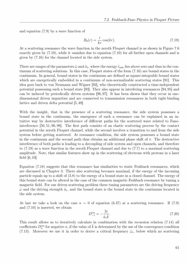
7.2. Feshbach-Fano Physics in Floquet Picture
and equation (7.9) by a wave function of
R0(r) =i
krcos(kr). (7.19)
At a scattering resonance the wave function in the zeroth Floquet channel is as shown in Figure 7.6exactly given by (7.19), while it vanishes due to equation (7.10) for all further open channels and isgiven by (7.16) for the channel located in the side system.
There are ranges of the parameters ω and a1, where the energy εside lies above zero and thus in the con-tinuum of scattering solutions. In this case, Floquet states of the form (7.16) are bound states in thecontinuum. In general, bound states in the continuum are defined as square-integrable bound stateswhich are energetically embedded in a continuum of non-normalizable scattering states [91]. Thisidea goes back to von Neumann and Wigner [92], who theoretically constructed a time-independentpotential possessing such a bound state [93]. They also appear in interfering resonances [94,95] andcan be induced by periodically driven systems [96, 97]. It has been shown that they occur in one-dimensional driven impurities and are connected to transmission resonances in both tight-bindinglattice and driven delta potential [5, 49].
With the insight, that in the presence of a scattering resonance, the side system possesses abound state in the continuum, the emergence of such a resonance can be explained in an in-tuitive way by destructive interference of different paths for the scattered wave related to Fano-interference [50, 51, 90, 98]. The first path consists of an elastic scattering process by the contactpotential in the zeroth Floquet channel, while the second involves a transition to and from the sidesystem before getting scattered. At resonance condition, the side system possesses a bound statein the continuum and the second path thus obtains an additional phase shift of π. The destructiveinterference of both paths is leading to a decoupling of side system and open channels, and thereforeto (7.19) as a wave function in the zeroth Floquet channel and due to (7.7) to a maximal scatteringamplitude. Note, that similar features show up in the scattering of electrons with protons in a laserfield [6, 10].
Equation (7.18) suggests that this resonance has similarities to static Feshbach resonances, whichare discussed in Chapter 3. There also scattering becomes maximal, if the energy of the incomingparticle equals up to a shift of (3.8) to the energy of a bound state in a closed channel. The energy ofthis bound state can be altered in the case of the common magnetic Feshbach resonance by tuning amagnetic field. For our driven scattering problem these tuning parameters are the driving frequencyω and the driving strength a1, and the bound state is the bound state in the continuum located inthe side system.
At last we take a look on the case n = 0 of equation (6.37) at a scattering resonance. If (7.9)and (7.10) is inserted, we obtain
Dres−1 = − 2i
a1k. (7.20)
This result allows us to iteratively calculate in combination with the recursion relation (7.14) allcoefficients Dres
n for negative n, if the value of k is determined by the use of the convergence condition(7.13). Moreover we use it in order to derive a critical frequency ωc, below which no scattering
61

7. Enhancement of Scattering by Periodic Driving
resonances occur. This is done by arguing, that the n = −1 Floquet channel is open if ε ≥ ~ω, dueto dispersion relation (5.17). In this case condition (7.10) also applies to the n = −1 channel andit states that Dres
−1 = 0, which is a contradiction to (7.20), as both a1 and k are not considered tobe infinitely large, so that equation (7.20) could not become zero. Due to this reasoning scatteringresonances can only occur for frequencies larger than the critical frequency ωc of Floquet energydivided by ~
ω ≥ ωc =ε
~. (7.21)
This feature has also been observed in scattering by an one-dimensional driven impurity [5, 98, 99]and is related to the opening of the Floquet channel with number n = −1. If condition (7.21) isnot fulfilled, the side system does not include the Floquet channel with number n = −1 and istherefore not directly coupled to the zeroth Floquet channel, where the incoming wave is present. Inthis situation the side system can not be decoupled from the open Floquet channels. As it turnedout that this decoupling of open and closed channels is essential for the emergence of a scatteringresonance, this explains the absence of resonances for frequencies below the critical one (7.21).
7.3. Investigation of Resonance Positions
We now use equation (7.14) to calculate the locations εres or εside, respectively, of the scatteringresonances in the ω-a1 plane. In Subsection 7.3.1 we do the calculation with a numerical method,while in 7.3.2 we work out an analytic approximation in the limit of weak driving.
7.3.1. Numerical Calculation
In order to solve equation (7.14) numerically, we first map it to a set of linear equations of infinitesize similar to (6.37), which reads
AD = 0, (7.22)
where the vector D consists of the coefficients Dn and the matrix elements of A vanish except of
An,n =i
kn− 1, (7.23)
An,n±1 = − a1
2. (7.24)
Like in equation (7.14) all indices n are restricted to the set n ∈ −N. In contrast to (6.43) thisequation is homogeneous. In this case a non-zero, and therefore physical, solution of the set of linearequations is only occurring, if the determinant of the matrix A vanishes. In order to compute sucha determinant numerically, we truncate the infinitely large matrix to a finite one by restricting theindex to be larger than a cut off m ∈ −N. This is appoximately valid due to condition (7.13). Weuse a Matlab algorithm to locate the zeros of the determinant and therefore the resonance positions.
62

7.3. Investigation of Resonance Positions
0.2 0.4 0.6 0.8 1 1.2 1.4 1.6
-1
-0.5
0
0.5
1
Figure 7.7.: Plot of the energy of the bound state of the side system εside (red) andthe Floquet scattering amplitude ascatt (blue, in arbitrary units) over the drivingfrequency for a1 = 0.3. The intersection of εside with the dotted line at ε = 0 equalsthe position of the scattering resonances for ascatt. We only calculated εside in thecase of ~ω > εside, as otherwise no resonances occur.
For energies larger than the driving frequency the imaginary part of the determinant gets non-zero.This indicates, that in this case the wave vector k−1 gets real and therefore the side system beginsat index n = −2. This results in the absence of scattering resonances in this region, as it representsthe case of driving frequencies lower than the critical one (7.21).
In Figure 7.7 we plot the energy εside over the driving frequency for fixed a1. This makes thestatement of equation (7.18) directly visible: A scattering resonance, which is visualised by the di-vergence of ascatt painted in blue in Figure 7.7, emerges at driving frequencies, where the Floquetenergy ε = 0 equals the energy of the side system εside. In addition it shows that for certain drivingfrequencies the side system possesses more than one bound state.
The results of this method in the ω-a1 plane is shown in Figure 7.8, where we show in (a) thelines, where εside intersect the Floquet energy of ε = 0 and in (b) we show intersections with aFloquet energy of ε = 0.5. We restricted this investigation to five scattering resonances located atthe largest frequencies. In both Figures lines of scattering resonances exist, which all start in thecase of ε = 0 at the ω-axis with the slope zero and ascend in the case of rising a1. For ε = 0.5 onlythree lines reach the ω-axis, as the others would have reached it below the critical frequency ωcrit.This behaviour of the lines of resonances equals to the lines of in Figure 7.1.
It turns out that in the case of negative a this method gives the result, that in the whole ω-a1
plane no bound state exists, and due to relation (7.18) this explains that no scattering resonancesoccur.
63

7. Enhancement of Scattering by Periodic Driving
0.2 0.4 0.6 0.8a1
0
0.5
1
1.5
2
2.5
3
hω
(a)
0.2 0.4 0.6 0.8a1
0
0.5
1
1.5
2
2.5
3
hω
(b)
Figure 7.8.: Location of scattering resonances in the ω-a1 plane for ε = 0 (a)and ε = 0.5 (b). The first resonance is painted in blue, the second red, the thirdyellow, the fourth purple and the fifth green. The dashed black vertical line showsthe position of the critical frequency (7.21), below which no resonances occur.
7.3.2. Analytic Evaluation
This Subsection is devoted to an approximative analytic evaluation of the resonance position byexpanding the recursion (7.14) in orders of the driving strength a1. We therefore express (7.14) inthe form
GnDn −a1
2(Dn+1 +Dn−1) = 0, n ∈ −N, (7.25)
where Gn = 1/κn−1 and the subscript side is dropped at the coefficients Dn for simplicity. In orderto evaluate this equation systematically we perform a perturbative ansatz for the coefficients
Dn =∞∑α=0
aα1D(α)n . (7.26)
We first consider the limit of vanishing driving amplitude a1, whose asymptotic behaviour is deter-mined in zeroth order of a1. The recursion (7.25) decouples in this case and reads(
1
κn− 1
)D(0)n = 0. (7.27)
It has only a non-vanishing solution
D(0)n = δn,m, m ∈ −N, (7.28)
if the term in the brackets vanishes. This is the case if κn = 1 for some n ∈ −N, which can besimplified to
εres = −1− n~ωres, n = −1,−2, ...,−nmax. (7.29)
64

7.3. Investigation of Resonance Positions
0 0.2 0.4 0.6 0.8 1ǫ
0
20
40
60
80
100
nmax
Figure 7.9.: Number of resonances nmax reaching the ω axis over the energy ε. Forvanishing energy the number diverges to infinity.
Due to the critical frequency (7.21) there exits a maximal number of scattering resonances forvanishing a1, which can be calculated by inserting (7.29) into condition (7.21). This inequality canbe solved for n, yielding
|n| ≤ nmax, (7.30)
with nmax = b1 + 1/εc as the maximal number of resonances at vanishing a1. The quantity nmax
is plotted in Figure 7.9. For ε close to one, only one resonance exists, while this number goes toinfinity in the case of vanishing Floquet energy. For the case of ε = 0.5 three resonances reach theω-axis, as it is shown in Figure 7.8.
Equation (7.29) provides an intuitive interpretation of the bound states of the side system, whichstands on the right-hand side of this equation, as a field dressed version of the bound state of thestatic contact potential. Additionally a physical interpretation of the interfering paths, which createthe scattering resonance by a Fano-interference, becomes clearer. The first path is the direct scat-tering process on the contact interaction, while the second one involves a transition to the boundstate of the contact potential with an emission of |n| driving field quanta and a subsequent transitionback. Moreover, the resonance number, defined in Section 7.1, is given by |n|.
We now solve recursion (7.25) to the first order of a1. The perturbative approach leads to theinsight, that for a solution of the form (7.28) in zeroth order only the coefficients D(1)
m±1 are unequalfrom zero. In case of the first resonance, where n = −1, equation (7.25) reads in this order of a1(
G−1 −a1/2−a1/2 G−2
)(D
(0)−1 + a1D
(1)−1
a1D(1)−2
)=
(00
). (7.31)
This equation only possesses a non-vanishing solution, if the determinant of the matrix vanishes.This leads to
G−1G−2 =a2
1
4. (7.32)
65

7. Enhancement of Scattering by Periodic Driving
In order to solve this equation approximately, we solve it first for κ−1 and find
κ−1 =1
1 +a2
1
41
1κ−2−1
. (7.33)
This expression can be solved for the driving frequency. In this step we approximate κ−2 ≈√εres + 2
by assuming the driving frequency to be located near the first resonance by inserting equation (7.29)into κ−2. As an intermediate step we arrive at an expression for the driving frequency of the firstscattering resonance for small a1. This reads
~ωres ≈ εres +1(
1 +a2
1
41
1√εres+2
−1
)2 . (7.34)
Using the small-argument approximation 1/(1 + x)2 ≈ 1 − 2x we extract the term in the leadingorder of a1
~ωres ≈ εres + 1− 1
2
11√
εres+2− 1
a21. (7.35)
This equation corresponds to (7.29) with an additional term being quadratic in a1, which can beseen as a shift of the field dressed energy of the bound state due to a finite driving strength a1.Alternatively, the same result can be obtained by looking at a convergence condition of the sequencesimilar to [49]. Following the procedure of [49], we come to
2
a1
G−1 ≈a1
2G−1−2, (7.36)
as an intermediate step, which is equal to equation (7.32).
In the case of resonances belonging to n 6= −1, a similar result can be obtained by looking atthe determinant of the matrix Gn−1 −a1/2 0
−a1/2 Gn −a1/20 −a1/2 Gn+1
. (7.37)
Performing the same steps as in the case of n = −1, we calculate the location on the |n|-th reso-nance
~ωres =ε
|n|+
1
|n|1[
1 +a2
1
4
(1
1√εres(n+1
n −1)+n+1n
−1+ 1
1√εres(n−1
n −1)+n−1n
−1
)]2 , (7.38)
which can be simplified in leading order of a1 to
~ωres ≈εres
|n|+
1
|n|− 1
2|n|
11√
εres(n+1n−1)+n+1
n
− 1+
11√
εres(n−1n−1)+n−1
n
− 1
a21. (7.39)
Similar to (7.35) these equations state that the energy of the driving induced bound state andtherefore the resonant frequency can be changed by altering the driving strength a1, while (7.39)
66
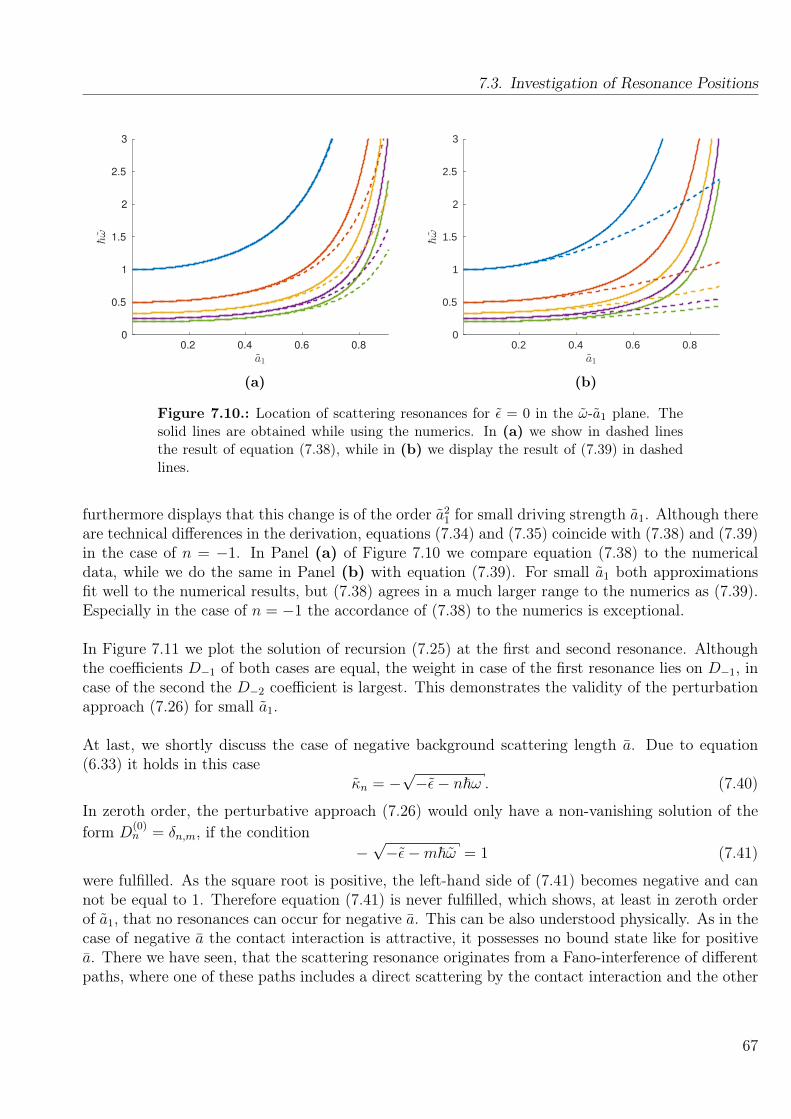
7.3. Investigation of Resonance Positions
0.2 0.4 0.6 0.8
a1
0
0.5
1
1.5
2
2.5
3
hω
(a)
0.2 0.4 0.6 0.8a1
0
0.5
1
1.5
2
2.5
3
hω
(b)
Figure 7.10.: Location of scattering resonances for ε = 0 in the ω-a1 plane. Thesolid lines are obtained while using the numerics. In (a) we show in dashed linesthe result of equation (7.38), while in (b) we display the result of (7.39) in dashedlines.
furthermore displays that this change is of the order a21 for small driving strength a1. Although there
are technical differences in the derivation, equations (7.34) and (7.35) coincide with (7.38) and (7.39)in the case of n = −1. In Panel (a) of Figure 7.10 we compare equation (7.38) to the numericaldata, while we do the same in Panel (b) with equation (7.39). For small a1 both approximationsfit well to the numerical results, but (7.38) agrees in a much larger range to the numerics as (7.39).Especially in the case of n = −1 the accordance of (7.38) to the numerics is exceptional.
In Figure 7.11 we plot the solution of recursion (7.25) at the first and second resonance. Althoughthe coefficients D−1 of both cases are equal, the weight in case of the first resonance lies on D−1, incase of the second the D−2 coefficient is largest. This demonstrates the validity of the perturbationapproach (7.26) for small a1.
At last, we shortly discuss the case of negative background scattering length a. Due to equation(6.33) it holds in this case
κn = −√−ε− n~ω . (7.40)
In zeroth order, the perturbative approach (7.26) would only have a non-vanishing solution of theform D
(0)n = δn,m, if the condition
−√−ε−m~ω = 1 (7.41)
were fulfilled. As the square root is positive, the left-hand side of (7.41) becomes negative and cannot be equal to 1. Therefore equation (7.41) is never fulfilled, which shows, at least in zeroth orderof a1, that no resonances can occur for negative a. This can be also understood physically. As in thecase of negative a the contact interaction is attractive, it possesses no bound state like for positivea. There we have seen, that the scattering resonance originates from a Fano-interference of differentpaths, where one of these paths includes a direct scattering by the contact interaction and the other
67

7. Enhancement of Scattering by Periodic Driving
-6 -5 -4 -3 -2 -1 0n
0
200
400
600
800
1000
1200
1400
1600
|Dn|
Figure 7.11.: Plot of the coefficients Dresn at the first (blue) and second (red)
resonance for a1 = 0.1 and ε = 0.01.
an additional transition to and from the bound state (A.14) of the contact potential. If the boundstate is not present, the second path does not exist, with the result of no possible interference ofpaths. This leads to the absence of scattering resonances as shown in Figure 7.4.
7.4. Scattering Amplitude in the Vicinity of a Resonance
In the last two Sections we only discussed the situation, where we are located exactly at the resonanceposition. In this Section we want to broaden the view and investigate the scattering amplitude inthe vicinity of a resonance. We already saw in Figures 7.2 and 7.4 that the shape of the scatteringamplitude around a resonance looks similar for different Floquet energies ε and driving strengths a1.This leads to the question, if this shape can be approximated by a simple formula, like it is done by(3.12) in the case of a magnetic Feshbach resonance. In order to give an answer to this question, weintroduce two phenomenological formulas, for which we show by fitting them to the data, that theyapproximate the shape of the scattering amplitude in the vicinity of a resonance. In Subsection 7.4.1we motivate the first formula as a frequency dependent adaption of equation (3.12) and compareit with the numerical data, while in Subsection 7.4.2 a second formula is derived by investigatingscattering in a two-channel model. In Section 7.5 we use these formulas in order to extract positionand width of the resonances by fitting the formulas introduced in this Section to the data.
7.4.1. Frequency Controlled Feshbach Scattering Amplitude
The first formula originates from equation (3.10). In the case of magnetic Feshbach resonances thebound-state energy ER in equation (3.10) is parametrised by ER = δµ(B − B0). Inspired by this
68

7.4. Scattering Amplitude in the Vicinity of a Resonance
approach we assume also a linear dependency of the bound state energy on the driving frequency
ER = C~(ω − ω0), (7.42)
where ω0 denotes the resonant frequency and C is a constant. Inserting this into equation (3.10)yields
− f0(ω) = abg
(1− ∆
~ω − ~ω0 − iΓ
). (7.43)
We additionally extrapolate the scattering length to the negative scattering amplitude in the caseof non-vanishing energy of the scattered particle. The involved parameters will be used as fittingparameters and have the following physical meaning. The background scattering length abg equalsthe scattering length in the limit of large frequencies, ∆ equals the width of the real part of theresonance in the limit of vanishing Γ. The quantity Γ limits the maximal amount of scattering anddetermines the width of the imaginary part. We introduce the dimensionless variable
x = ~ω − ω0
∆(7.44)
and separate equation (7.43) in real and imaginary part
−Re f0(ω)
abg
= 1 +x
x2 +(
Γ∆
)2 (7.45)
−Im f0(ω)
abg
=∆
Γ
1(xΓ
)2+ 1
. (7.46)
In Figure 7.12 we compare these formulas to the numerical data by fitting both real and imaginarypart simultaneously. In general, we obtain a good agreement between both, deviations are muchsmaller than the actual values.
69

7. Enhancement of Scattering by Periodic Driving
-0.05 0 0.05
(hω − hω0)/∆
-80
-60
-40
-20
0
20
40
−f 0
(a)
-5 0 5
(hω − hω0)/∆ ×10-4
-8000
-6000
-4000
-2000
0
2000
4000
−f 0
(b)
-0.05 0 0.05
(hω − hω0)/∆
-80
-60
-40
-20
0
20
40
−f 0
(c)
0 0.01 0.02 0.03 0.04
(hω − hω0)/∆
-50
-45
-40
-35
-30
-25
-20
−f 0
(d)
Figure 7.12.: Comparison of the real (blue) and imaginary (red) part of the scatter-ing amplitude −f0 over the difference of the driving frequency ω from the resonantω0 measured in units of the width ∆. The values for fitting equation (7.43) are shownwith + for real and o for imaginary part. Panel (a) shows the case of ε = 10−4 anda1 = 0.1, which gave the result of ~ω0 = 1.0174, ∆ = 5.0673×10⁻³, Γ = 5.0260 10−5
and abg = 0.9917. Panel (b) shows the case of ε = 10−8 and a1 = 0.1, which gave theresult of ~ω0 = 1.0173, ∆ = 5.064× 10⁻³, Γ = 5.025×10⁻⁷ and abg = 0.992. Panel(c) shows the case of ε = 10−4 and a1 = 0.5, which gave the result of ~ω0 = 1.6135,∆ = 0.1671, Γ = 1.5×10⁻³ and abg = 0.9. Panel (d) shows an enlarged plot of case(a) in order to indicate the limitations of the method.
In (b) we decreased the Floquet energy ε compared to (a). While the width ∆ stays approximatelythe same, the maximal enhancement of scattering is larger, while the scaling of the frequency axis bya factor of 10−2 has to be done in order to resolve the shape of the resonance in a way like it is donein (b). This behaviour is implemented in equation (7.46), as Γ also changes with 10−2, which leadswith equation (7.46) to an enhancement of the maximum by 102. In addition, (7.46) is expressed ina way, where it only depends on x/Γ, which makes visible, that the scaling of the x-axis leads toa similar shape of the imaginary part of the scattering amplitude. The real part (7.45) has similar
70

7.4. Scattering Amplitude in the Vicinity of a Resonance
1.07208 1.0721 1.07212 1.07214 1.07216 1.07218hω
-50
-49.8
-49.6
-49.4
-49.2
-49
-48.8
−f0(ω
)
1.06 1.08 1.1
-80-60-40-20
02040
(a)
1.075 1.08 1.085 1.09 1.095 1.1hω
-0.1
-0.05
0
0.05
0.1
−f0(ω
)
1.06 1.08 1.1
-80-60-40-20
02040
(b)
Figure 7.13.: Enlarged plots of real (blue) and imaginary (red) part of the scatteringamplitude calculated with the numerical method of Subsection 6.4.1. The black areain the inset points out the enlarged area. The black dotted line in panel (b) is aguide to the eye. Both plots are calculated with ε = 10−4 and a1 = 0.2.
scaling properties. In (c) we increased a1 compared to (b), here the curve looks the same like in (b)and the value of ∆/Γ stays approximately the same. This behaviour is also included in equations(7.45) and (7.46), as (7.45) depends on ∆/Γ, while (7.46) has slight deviations. Panel (d) showsthat equation (7.45) deviates largest from the data around the maximum value of the real part. Inorder to see this more detailed, we show in Figure 7.13 (a) an enlarged plot of the numerical data,which fulfil the relation
2 max |Re f0| = max |Im f0|, (7.47)
but equation (7.43) does that explicitly not. This shows a limitation of the fitting with equation(7.43).
As it is useful in the later discussion, we calculate the limit of vanishing Γ of equations (7.45)and (7.46). The imaginary part (7.46) is proportional to a Lorentz-shaped curve with width Γ.Therefore in the limit Γ→ 0 it is proportional to the Dirac-delta function. Both real and imaginarypart of the scattering amplitude read in the limit of vanishing Γ
− limΓ→0
Re f0
abg
= 1− 1
x, (7.48)
− limΓ→0
Imf0
abg
= −∆πδ(~ω − ~ω0) (7.49)
Equation (7.48) equals (3.12), if the magnetic field is replaced by the driving frequency ω. Butinstead of being zero, the imaginary part is proportional to the Dirac-Delta function in this limit.
71
7. Enhancement of Scattering by Periodic Driving
7.4.2. Scattering Amplitude of a Simple Coupled Channel Model
In the spirit of the radial Floquet equation (6.11) the scattering by a time-dependent potential canbe rewritten as a multi-channel scattering problem. For the derivation of the second approximativeformula, we ask the question, how many channels are necessary in order to approximate the physics ofFloquet scattering, which intrinsically involves an infinite amount of channels. As the simplest non-trivial model we investigate the scattering by a two-channel Hamiltonian with contact interaction
H(r) = H0(r) + Vint(r). (7.50)
Here H0 consists of the kinetic energy and the intra-channel potential
H0 = − ~2
2µ
(1r2
∂∂rr2 ∂
∂r0
0 1r2
∂∂rr2 ∂
∂r
)+
~2
2µ
(2a0
r2 δ(r)∂∂rr 0
0 V + 2a1
r2∂∂rr
), (7.51)
where the zeroth channel is considered to be open, while the energy of the first channel is shifted byV in order to obtain a closed one. If we only consider H0 as the Hamiltonian, the two channels aredecoupled, and the scattering by H0 is described with the findings of Appendix A. In this case thescattering amplitude in the zeroth channel is −f−1 = 1/a0 + ik and the first one possesses a boundstate with the eigenenergy
Ebound = V − 1/a21. (7.52)
The inter-channel coupling is induced by the potential
Vint(r) =~2
2µ
(0 2aWW
r2 δ(r) ∂∂rr
2aWW
r2 δ(r) ∂∂rr 0
). (7.53)
The strength of the coupling is given by aWW, which has the dimension of a scattering length.
If one would only consider the Floquet channels n = 0 and n = −1 in the radial Floquet equa-tion in coupled channel representation (6.11), one would recover the same Hamilton operator as(7.50), but with the parameters a0 = a1 = a, aWW = a1a and V = ~ω. In this model we wantto go beyond and absorb the influence of higher Floquet channels of the side system in a1, whichdoes not have to be related to a0, and a potential of the form V = |n|~ω. In Appendix C wederive the scattering amplitude of model (7.50) and see, that the inverse scattering amplitude canbe approximated by the form
− 1
f=
1
aBG
ω − ω0
ω − ω0 − δ/~+ iγ, (7.54)
where we have introduced by
aBG = a0
(1− a2
WW
a0a1
), (7.55)
the background scattering length, which determines the scattering amplitude in the case of aninfinitely large frequency ω. The width of the real part of the scattering amplitude corresponds to
δ =2a2
WW
a0a1|n|1
1− a2WW
a0a1
1
a21
. (7.56)
72

7.4. Scattering Amplitude in the Vicinity of a Resonance
The quantity
γ = k (7.57)
characterises the width of the imaginary part and its inverse corresponds to the maximal value ofthe scattering amplitude. In practice, ω0, δ, γ and aBG are fitting parameters and are extractedby fitting equation (7.54) to the numerical data for f0. We can invert relations (7.55)-(7.57) incombination with (7.52) in order to calculate the parameters of the simple coupled channel modelfrom the fitting parameters obtained with equation (7.54). The inverted relations read
E = γ2, (7.58)
a1 =
√1
−E + |n|~ω0
, (7.59)
aWW =
√1
2aBGδa3
1|n| , (7.60)
a0 = aBG +a2
WW
a1
. (7.61)
Formula (7.54) has been reported recently by [80], but without the derivation shown in AppendixC. With the dimensionless variable
x = ~ω − ω0
δ(7.62)
the scattering amplitude (7.54) is expressed in real and imaginary part
−Re faBG
=(x− 1)x
x2 + γ2a2BG(x− 1)2
, (7.63)
−Im f
aBG
= − γaBG(x− 1)2
x2 + γ2a2BG(x− 1)2
. (7.64)
In Figure 7.14 we compare these equations to the numerical data by simultaneously fitting real andimaginary part. Similar to Figure 7.12 we find a good agreement between approximative formula andnumerical data. Panel (d) shows that equation (7.54) resolves the numerical data in the vicinity ofthe maximum of the real part, which is a benefit in comparison to equation (7.43). Also in this casewe scaled both axis in order to plot the scattering amplitude for different parameters in a similarform.
73

7. Enhancement of Scattering by Periodic Driving
-0.05 0 0.05
(hω − hω0)/δ
-80
-60
-40
-20
0
20
40
−f 0
(a)
-5 0 5
(hω − hω0)/δ ×10-4
-8000
-6000
-4000
-2000
0
2000
4000
−f 0
(b)
-0.05 0 0.05
(hω − hω0)/δ
-80
-60
-40
-20
0
20
40
−f 0
(c)
0 0.01 0.02 0.03 0.04
(hω − hω0)/δ
-50
-40
-30
-20
-10
0−f 0
(d)
Figure 7.14.: Comparison of the real (blue) and imaginary (red) part of the scatter-ing amplitude −f0 over the difference of the driving frequency ω from the resonantω0 measured in units of the width ∆. The values for fitting equation (7.43) are shownwith + for real and o for imaginary part. Panel (a) shows the case of ε = 10−4 anda1 = 0.1, which gave the result of ~ω0 = 1.0174, δ = 5.051 × 10⁻³, γ = 10−2 andabg = 0.995. Panel (b) shows the case of ε = 10−8 and a1 = 0.1, which gave theresult of ~ω0 = 1.0173, δ = 5.0507 × 10⁻³, γ = 10−4 and abg = 0.995. Panel (c)shows the case of ε = 10−4 and a1 = 0.5, which gave the result of ~ω0 = 1.6135,δ = 0.1826, γ = 10−2 and abg = 0.8235. Panel (d) shows an enlarged plot of thecase of (a).
The invariance between (a) and (c) is directly implemented in equations (7.63) and (7.64), as theyare completely expressed by the dimensionless variable x. Because
maxRe |f | = 1
2γ(7.65)
andmax Im |f | = 1
γ(7.66)
74

7.5. Position and Width of Scattering Resonances
hold for equations (7.63) and (7.64), we see in Panel (b), that a larger enhancement of scattering isdescribed by a lower value of γ. In Figure 7.13 (b) we see that only the real part of the numericallycalculated scattering amplitude has a zero, while (7.63) and (7.64) only simultaneously equal zero.This is a limitation of these approximate formulas.
Since it is important in the next Section, we show in Appendix D that for the limit of vanishingwidth γ formulas (7.63) and (7.64) converge to
− limγ→0
Re f = aBG
(1− δ
~ω − ~ω0
). (7.67)
for the real and− lim
γ→0Im f(ω) = −|δ|aBGπδ(ω − ω0). (7.68)
for the imaginary part. The real part fits with the corresponding result of (7.48), while the imaginarydiffers from (7.49) only by a modulus of δ.
7.5. Position and Width of Scattering Resonances
In this Section we use both equations (7.43) and (7.54) in order to extract fitting parameters charac-terising the scattering resonance. In particular we are interested in the position ~ω0 and the width∆ or δ. In Subsection 7.5.1 we evaluate the dependency of the fitting parameters on the Floquetenergy ε, while in Subsection 7.5.2 we evaluate their values in the ω-a1 plane.
7.5.1. Energy Dependence of Parameters
We now investigate the behaviour of the fitting parameters, which characterise a resonance. Wetherefore fit the formulas (7.43) and (7.54) to the numerical data and extract the dependencies oftheir parameters on the Floquet energy ε. As the coefficient of determination R2 [100] quantifiesthe accordance between the results of the fitting procedure to the data, only those fits yielding acoefficient of determination R2 close to one are considered. The closer R2 lies by one, the better thefit explains the data. We start with the width of the imaginary parts γ, respectively, Γ and foundout that they depend on the Floquet energy in the following way
log γ = p1 log ε+ p2, (7.69)log Γ = p1 log ε+ p2. (7.70)
We display this result in Figure 7.15 (a). In Table 7.1 we see, that p1 ≈ 0.5, which implies thedependency of γ on ε by
γ ≈√ε , (7.71)
while in the case of equation (7.43) one has to multiply the right-hand side by a constant C = 10p1 ,
75
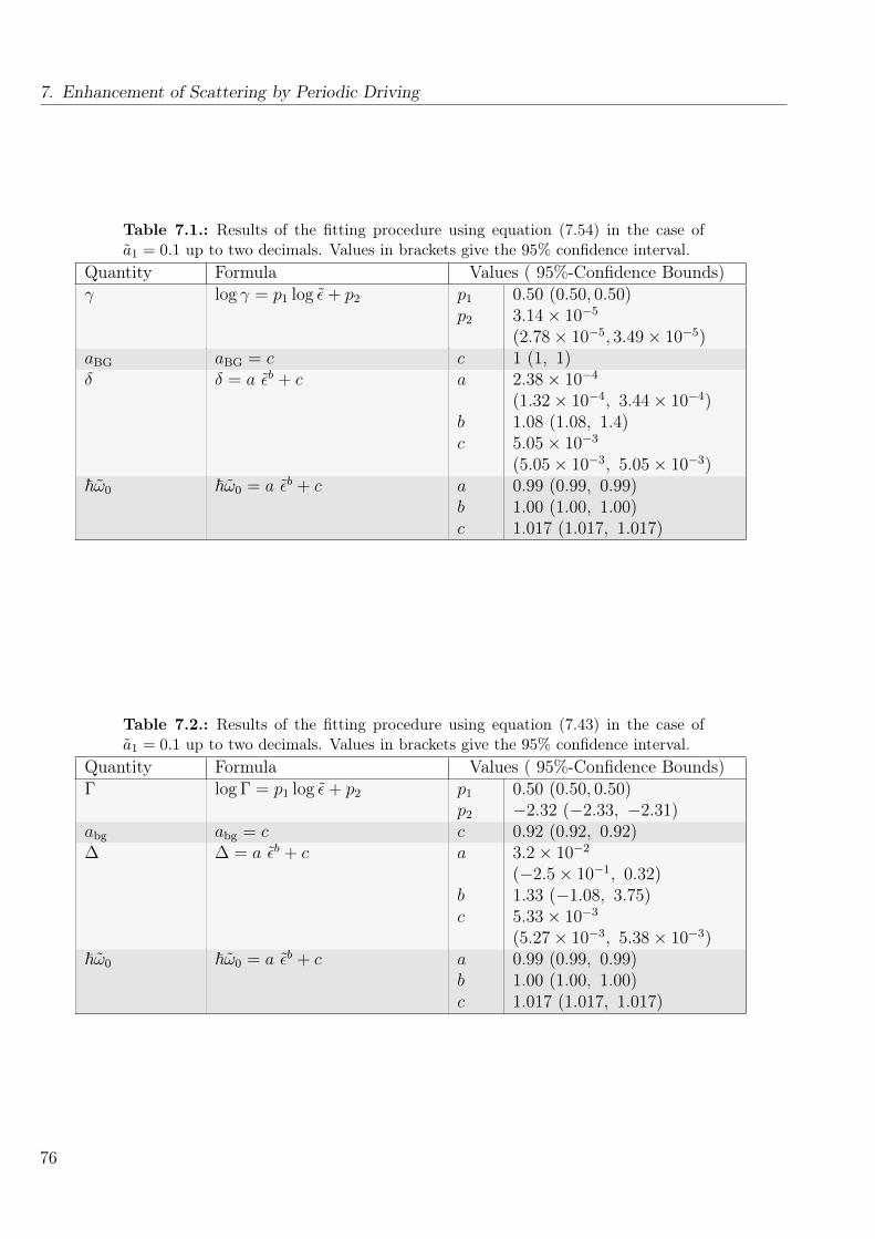
7. Enhancement of Scattering by Periodic Driving
Table 7.1.: Results of the fitting procedure using equation (7.54) in the case ofa1 = 0.1 up to two decimals. Values in brackets give the 95% confidence interval.
Quantity Formula Values ( 95%-Confidence Bounds)γ log γ = p1 log ε+ p2 p1
p2
0.50 (0.50, 0.50)3.14× 10⁻⁵
(2.78× 10⁻⁵, 3.49× 10⁻⁵)aBG aBG = c c 1 (1, 1)δ δ = a εb + c a
bc
2.38× 10⁻⁴
(1.32× 10⁻⁴, 3.44× 10⁻⁴)1.08 (1.08, 1.4)5.05× 10⁻³
(5.05× 10⁻³, 5.05× 10⁻³)~ω0 ~ω0 = a εb + c a
bc
0.99 (0.99, 0.99)1.00 (1.00, 1.00)1.017 (1.017, 1.017)
Table 7.2.: Results of the fitting procedure using equation (7.43) in the case ofa1 = 0.1 up to two decimals. Values in brackets give the 95% confidence interval.
Quantity Formula Values ( 95%-Confidence Bounds)Γ log Γ = p1 log ε+ p2 p1
p2
0.50 (0.50, 0.50)−2.32 (−2.33, −2.31)
abg abg = c c 0.92 (0.92, 0.92)∆ ∆ = a εb + c a
bc
3.2× 10⁻²
(−2.5× 10⁻¹, 0.32)1.33 (−1.08, 3.75)5.33× 10⁻³
(5.27× 10⁻³, 5.38× 10⁻³)~ω0 ~ω0 = a εb + c a
bc
0.99 (0.99, 0.99)1.00 (1.00, 1.00)1.017 (1.017, 1.017)
76

7.5. Position and Width of Scattering Resonances
-8 -6 -4 -2
log(ǫ)
-7
-6
-5
-4
-3
-2
-1
log(γ)resp.log(Γ)
(a)
-8 -6 -4 -2
log ǫ
1
1.02
1.04
1.06
1.08
1.1
hω
(b)
Figure 7.15.: Panel (a) shows in blue the results of the fitting parameter γ of (7.54)and in yellow the results for Γ defined in (7.43). Linear fits for both data are shownin dashed lines. Panel (b) shows position ~ω0 and width δ (dashed lines) obtainedwith equation (7.54) of the first scattering resonance.
which is documented in Table 7.2 and gets
Γ = C√ε . (7.72)
Further investigations revealed, that equations (7.71) and (7.72) stay true in the case of larger a1,while the constant C depends on a1.
As the main result of this investigation we can state that in the limit of vanishing energy ε both γ andΓ are going to zero and therefore equations (7.63), (7.64) and (7.48), (7.49) are a valid description ofthe scattering resonance in the limit of vanishing Floquet energy ε. As in both cases the imaginarypart of the Floquet-scattering length is proportional to a Dirac-delta function, we conclude that theFloquet scattering resonance is lossless if the driving frequency does not exactly hit the resonantfrequency ~ω0. One leading physical mechanism of losses is inelastic scattering. We show in Section7.2 that all higher open Floquet channels possess a vanishing Floquet scattering length, which meansthat at scattering resonance inelastic collisions are not present.
We found out that the behaviour of the quantity ~ω0 as shown in Figure 7.15 is described by apower law
Q = a εb + c. (7.73)
In the case of aBG, abg, δ and ∆ a power law gives only the trend of the data and does not match toeach single data point, as shown in Figure 7.16. The result of this investigation is shown in Tables7.1 and 7.2. In Figure 7.15 (b) we see that both position and width stay approximately constantfor Floquet energies below ε = 10−4.
As the coefficient of determination R2 [100] quantifies the accordance between the results of thefitting procedure to the data, we compare the values of R2 between (7.43) and (7.54). In Figure 7.16
77

7. Enhancement of Scattering by Periodic Driving
-10 -8 -6 -4 -2 0
log ǫ
5.048
5.05
5.052
5.054
5.056
5.058
5.06
5.062
5.064
δ
×10-3
(a)
-8 -6 -4 -2
log(ǫ)
-10
-8
-6
-4
-2
log(1−R
2)
(b)
Figure 7.16.: (a): Plot of the fitting parameter δ (blue) and a power law fit (red).(b): plot of the decade logarithm of 1 − R2 of the fit results with equation (7.54)(blue) and equation (7.43) (red) relative to the decade logarithm of the Floquetenergy ε in the case of a1 = 0.1.
we plot the logarithm of 1 − R2. The coefficient of determination gets closer to one in the case ofvanishing Floquet energy ε, signalling a better accordance of the fitting equations to the numerics.Additionally the values corresponding to (7.54) are always closer to one and therefore fit better to thedata than the ones, which correspond to (7.43). We conclude that equation (7.54) is more suitablein order to describe the shape of a scattering resonance than (7.43). This is additionally manifestedin numerical instabilities occurring in the fit results of equation (7.43) in the case of small Floquetenergies ε and by the findings displayed in Panel (d) of Figures 7.12 and 7.14.
7.5.2. Position and Width in the ω-a1 Plane
After the investigation of the ε dependence of the scattering-resonance parameters we take a look onthe behaviour of these resonances in the ω-a1 plane. We specialise to the case of vanishing Floquetenergy. In order to calculate the numerical results, we use equation (6.42), which is valid for ε = 0.Due to the considerations in the previous Subsection, we do a fitting procedure using equation (7.67).In Figure 7.17 we compare equation (7.67) to the numerical data and obtain a good agreement. Itturns out that this fitting procedure yields good results, except for small values of a1, as in this casethe resonances become very narrow and the fitting procedure fails due to computational issues. Inorder to obtain results also in this region, we extrapolated the data to small a1 and excluded datapoints with a large numerical uncertainty. This can be done with a high precision, as the resonancefrequency at a1 = 0 is known due to equation (7.29). As a result, we plot in Figure 7.18 positionand width of the first five resonances in the ω-a1 plane. Similar to Figure 7.8 the resonance positionsand widths increase for larger a1. Figure 7.18 can be seen as a map of how to tune the parametersin order to form the shape of the resonance in a desired way. The time-averaged scattering length a
78
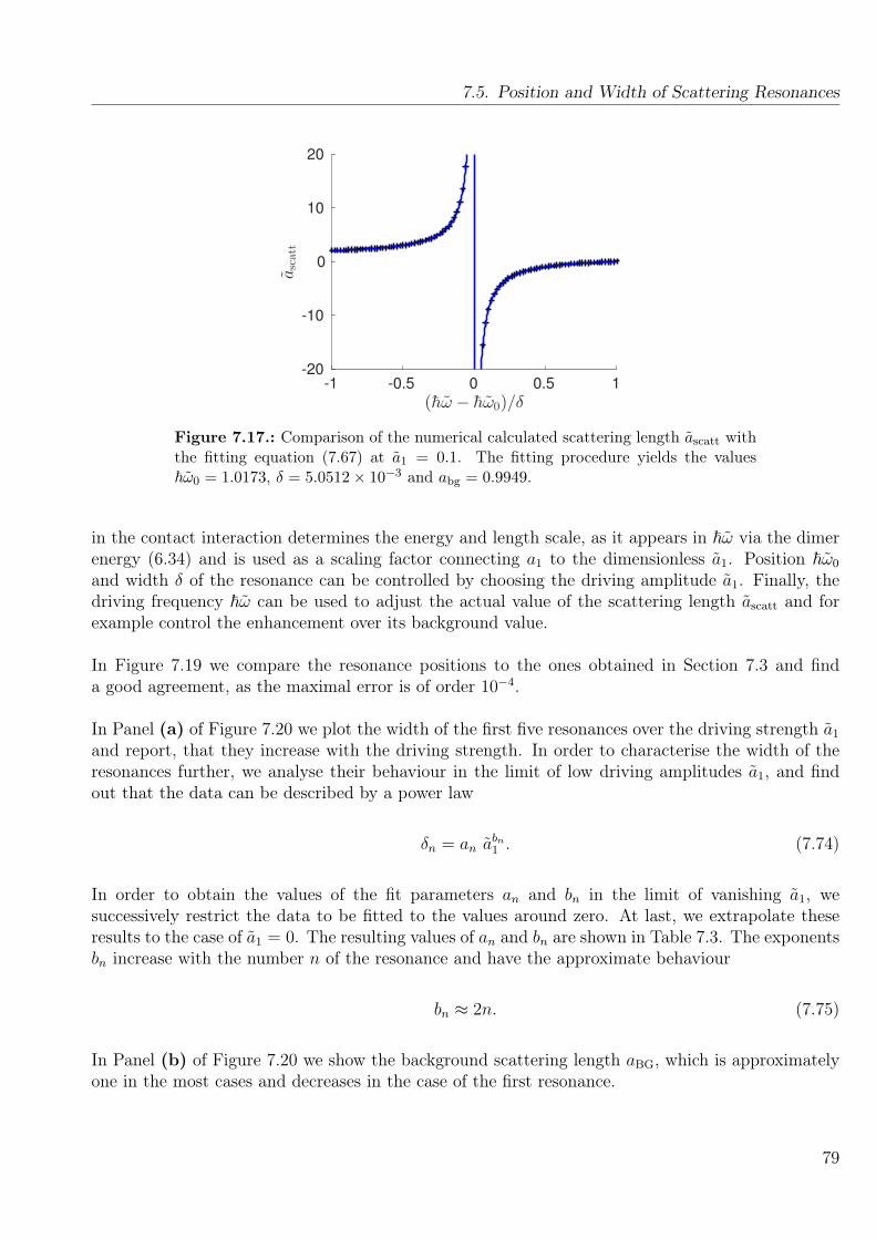
7.5. Position and Width of Scattering Resonances
-1 -0.5 0 0.5 1
(hω − hω0)/δ
-20
-10
0
10
20
ascatt
Figure 7.17.: Comparison of the numerical calculated scattering length ascatt withthe fitting equation (7.67) at a1 = 0.1. The fitting procedure yields the values~ω0 = 1.0173, δ = 5.0512× 10⁻³ and abg = 0.9949.
in the contact interaction determines the energy and length scale, as it appears in ~ω via the dimerenergy (6.34) and is used as a scaling factor connecting a1 to the dimensionless a1. Position ~ω0
and width δ of the resonance can be controlled by choosing the driving amplitude a1. Finally, thedriving frequency ~ω can be used to adjust the actual value of the scattering length ascatt and forexample control the enhancement over its background value.
In Figure 7.19 we compare the resonance positions to the ones obtained in Section 7.3 and finda good agreement, as the maximal error is of order 10−4.
In Panel (a) of Figure 7.20 we plot the width of the first five resonances over the driving strength a1
and report, that they increase with the driving strength. In order to characterise the width of theresonances further, we analyse their behaviour in the limit of low driving amplitudes a1, and findout that the data can be described by a power law
δn = an abn1 . (7.74)
In order to obtain the values of the fit parameters an and bn in the limit of vanishing a1, wesuccessively restrict the data to be fitted to the values around zero. At last, we extrapolate theseresults to the case of a1 = 0. The resulting values of an and bn are shown in Table 7.3. The exponentsbn increase with the number n of the resonance and have the approximate behaviour
bn ≈ 2n. (7.75)
In Panel (b) of Figure 7.20 we show the background scattering length aBG, which is approximatelyone in the most cases and decreases in the case of the first resonance.
79
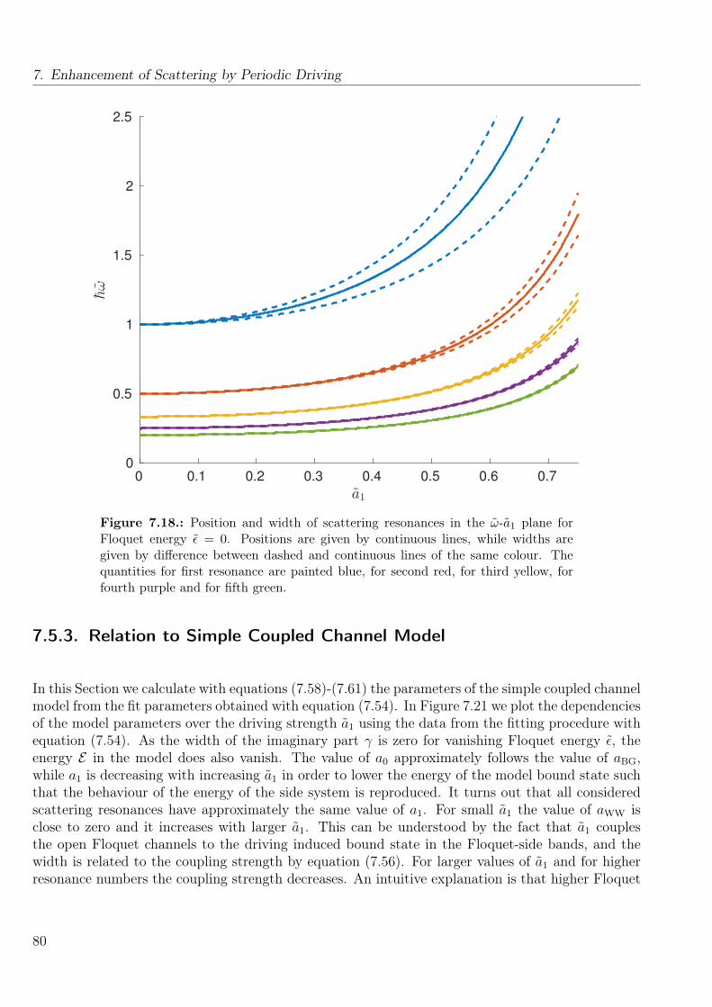
7. Enhancement of Scattering by Periodic Driving
0 0.1 0.2 0.3 0.4 0.5 0.6 0.7
a1
0
0.5
1
1.5
2
2.5
hω
Figure 7.18.: Position and width of scattering resonances in the ω-a1 plane forFloquet energy ε = 0. Positions are given by continuous lines, while widths aregiven by difference between dashed and continuous lines of the same colour. Thequantities for first resonance are painted blue, for second red, for third yellow, forfourth purple and for fifth green.
7.5.3. Relation to Simple Coupled Channel Model
In this Section we calculate with equations (7.58)-(7.61) the parameters of the simple coupled channelmodel from the fit parameters obtained with equation (7.54). In Figure 7.21 we plot the dependenciesof the model parameters over the driving strength a1 using the data from the fitting procedure withequation (7.54). As the width of the imaginary part γ is zero for vanishing Floquet energy ε, theenergy E in the model does also vanish. The value of a0 approximately follows the value of aBG,while a1 is decreasing with increasing a1 in order to lower the energy of the model bound state suchthat the behaviour of the energy of the side system is reproduced. It turns out that all consideredscattering resonances have approximately the same value of a1. For small a1 the value of aWW isclose to zero and it increases with larger a1. This can be understood by the fact that a1 couplesthe open Floquet channels to the driving induced bound state in the Floquet-side bands, and thewidth is related to the coupling strength by equation (7.56). For larger values of a1 and for higherresonance numbers the coupling strength decreases. An intuitive explanation is that higher Floquet
80
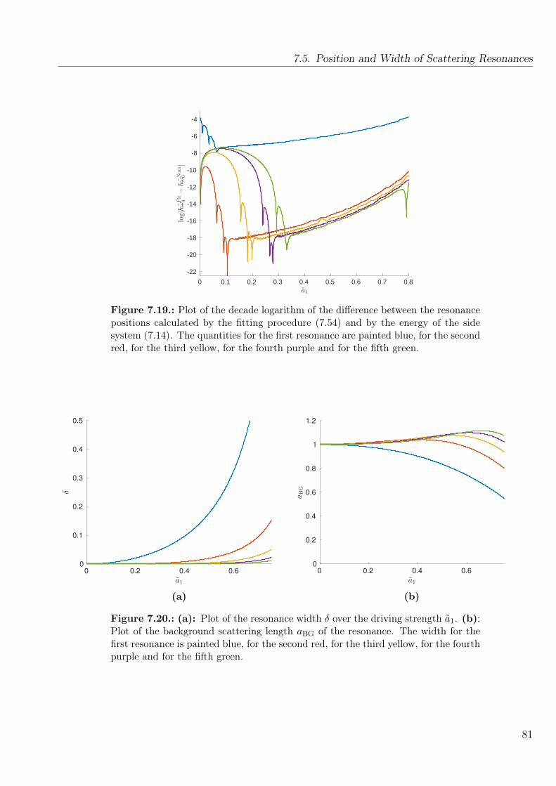
7.5. Position and Width of Scattering Resonances
0 0.1 0.2 0.3 0.4 0.5 0.6 0.7 0.8a1
-22
-20
-18
-16
-14
-12
-10
-8
-6
-4
log|hωFit
0−hωNum
0|
Figure 7.19.: Plot of the decade logarithm of the difference between the resonancepositions calculated by the fitting procedure (7.54) and by the energy of the sidesystem (7.14). The quantities for the first resonance are painted blue, for the secondred, for the third yellow, for the fourth purple and for the fifth green.
0 0.2 0.4 0.6
a1
0
0.1
0.2
0.3
0.4
0.5
δ
(a)
0 0.2 0.4 0.6
a1
0
0.2
0.4
0.6
0.8
1
1.2
aBG
(b)
Figure 7.20.: (a): Plot of the resonance width δ over the driving strength a1. (b):Plot of the background scattering length aBG of the resonance. The width for thefirst resonance is painted blue, for the second red, for the third yellow, for the fourthpurple and for the fifth green.
81

7. Enhancement of Scattering by Periodic Driving
Table 7.3.: Results of the fitting procedure for widths of the resonances δ = a ab1in the limit of vanishing a1 up to two decimals. Values in brackets give the 95%confidence bounds.Number an bn1 0.48 (0.44, 0.55) 2.00 (1.97, 2.03)2 0.36 (0.32, 0.39) 4.00 (3.97, 4.02)3 0.34 (0.26, 0.42) 5.94 (5.83, 6.05)4 0.33 (0.19, 0.48) 7.79 (7.54, 8.05)5 0.42 (0.26, 0.58) 9.83 (9.63, 10.03)
0 0.2 0.4 0.6
a1
0
0.5
1
1.5
a0
(a)
0 0.2 0.4 0.6
a1
0.5
0.6
0.7
0.8
0.9
1
a1
(b)
0 0.2 0.4 0.6
a1
0
0.05
0.1
0.15
0.2
aW
W
(c)
Figure 7.21.: Plot of the parameters of the simple coupled channel model of Section7.4.2 over the driving strength a1. In (a) the background scattering length of thefree channel is plotted, in (b) the one for the closed and in (c) the coupling strengthof both channels, which are present in the model. Quantities for first resonance arepainted blue, for second red, for third yellow, for fourth purple and for fifth green.
82

7.6. Kramers-Kronig like Relation between Real and Imaginary Part
channels get more populated and therefore the overlap between the wave functions in different modesbecomes smaller. This results in an effective smaller coupling of the channels. Note that these modelparameters exist due to simplification issues and are no measurable quantities.
7.6. Kramers-Kronig like Relation between Real andImaginary Part
After the detailed analysis of the scattering resonances we report that the following quantity involvingthe time-averaged scattering amplitude
χ(ω) = −f0(ω) + limω→∞
f0(ω) (7.76)
fulfils the so called anti Kramers-Kronig relations
Re χ(ω0) = − 1
πP∫ ∞−∞
dωIm χ(ω)
ω − ω0
, (7.77)
Im χ(ω0) =1
πP∫ ∞−∞
dωRe χ(ω)
ω − ω0
, (7.78)
which are derived in Appendix B for anti-causal susceptibilities. We introduced the principal valueintegral as
P∫ ∞−∞
dxχ(x)
x− x0
= limγ→0
(∫ x0−γ
−∞dx+
∫ ∞x0+γ
dx
)χ(x)
x− x0
(7.79)
and use the quantity χ(ω) = −f0(ω) + limω→∞
f(ω) instead of the bare scattering amplitude −f0(ω) inorder to ensure that the limit of χ(ω) for infinite frequencies is going to zero. We show in AppendixB, that this condition is necessary for the fulfilment of the anti-Kramers Kronig relations. Thefact that (7.76) fulfils equations (7.77) and (7.78) is not a violation of causality, as (7.76) is not asusceptibility. The fulfilment of the anti-causal Kramers Kronig relations signals that the scatteringamplitude f0(ω) has a simple analytic structure, which captures the physics of a scattering reso-nance. In Appendix B we further show, that functions with poles in the upper complex half planefulfil the anti-Kramers Kronig relations. As both fit formulas (7.43) and (7.54) have only one pole,which is located in the upper half plane for positive γ or Γ, respectively, they also fulfil equations(7.77) and (7.78).
In order to show that the numerically calculated values fulfil the anti-Kramers-Kronig relations,a MATLAB function was implemented in order to calculate the imaginary part of the scatteringamplitude using the real part with equation (7.78) and vice versa with (7.77). The function is im-plemented in the following way: The integrals in (7.77) and (7.78) are truncated to a range of totallength 2Λ lying symmetrically around the point ω0. This is done in order to ensure that
P∫ Λ+ω0
−Λ+ω0
dw1
ω − ω0
= 0. (7.80)
83

7. Enhancement of Scattering by Periodic Driving
1.016 1.0165 1.017 1.0175 1.018 1.0185 1.019
hω
-100
-50
0
50
−f0(ω
)
Figure 7.22.: Plot of real (blue) and imaginary (red) part of the negative scatteringamplitude in the case of ε = 10−4, a1 = 0.1. The yellow + mark the values obtainedby re-calculating the real part using the imaginary by equation (7.77). The purplex are calculated using equation (7.78).
Additionally we approximate the principal value by leaving out the integration between the valuesω0 − εp and ω0 + εp, where εp is a small, but numerical resolvable value. The numerics have beenvalidated with the function χval(ω) = 1/(ω + iγ), which has a pole in the upper complex half planefor γ < 0 and therefore known to fulfil the anti-Kramers-Kronig relations.
The result of this investigation is shown in Figure 7.22, where a good agreement between numericaland anti-Kramers-Kronig relations calculated data is shown. In Figure 7.23 we plot the relativenorm
|χnumeric(ω)− χanti−Kramers−Kronig(ω)||χnumeric(ω)|
(7.81)
of the error between numerical and anti-Kramers-Kronig calculated data. For all considered posi-tions in the ε-a1 plane this error has the order of the numerical uncertainty of the method.
Additionally we can directly show that (7.43) and (7.54) fulfil the anti-Kramers-Kronig relationsin the case of positive imaginary part γ or Γ, respectively, by calculating the principal value integralin the following manner
P∫ ∞−∞
dxχ(x)
x− x0
= limγ→0,Λ→∞
(∫ x0−γ
−Λ+x0
dx+
∫ Λ+x0
x0+γ
dx
)χ(x)
x− x0
. (7.82)
It turns out that in the case of (7.43) and (7.54) both in equation (7.82) occurring limits commute.
84

7.7. Scattering Amplitude at Large Driving Frequencies
0.1 0.2 0.3 0.4 0.5
-8
-6
-4
-2
0
5
10
15
10-3
Figure 7.23.: Plot of the relative error (7.81) of numerical data and anti-Kramers-Kronig relation recalculated data in the plane of Floquet energy ε and drivingstrength a1.
7.7. Scattering Amplitude at Large Driving Frequencies
In this Section we consider the limit of infinitely large driving frequencies. In this case the wavefunctions in all Floquet channels with index greater than zero are unbound, while all below arebound. Interestingly, the coefficients Dn obey the rule Dn = D−n, as the recursion relation (6.49)is the same in both cases. Therefore the amplitude of the wave function in both open and closedFloquet channels are distributed symmetrically around channel number zero in this limit. Thescattering amplitude can be calculated with the results obtained in Section 6.4 by inserting equation(6.54) into (6.26) and it reads
f0(ε, a1) =−√
1− a21 + i(1− a2
1)k0
1 +√
1− a21 k0
. (7.83)
As equation (7.83) has no dependency on the driving frequency, this result corresponds to thelimit of infinite large driving frequency without any 1/ω correction. A plot of (7.83) in the ε-a1
plane is performed in Figure 7.24. If a1 = 1, real and imaginary part of the scattering amplitudevanishes. For the limit of ε going to zero the imaginary part vanishes, while the real part convergesto ascatt =
√1− a2
1 . This is quite remarkable, as for large driving frequencies one would expect, thatthe effect of the time-dependent part vanishes due to averaging issues, which leads to a scatteringlength of ascatt = 1. Additionally no resonances occur, as the condition of maximal scattering (7.7)can never be fulfilled by equation (7.83).
85
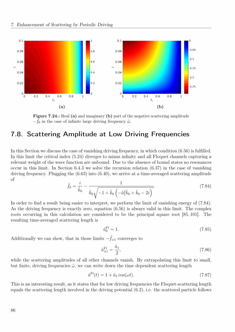
7. Enhancement of Scattering by Periodic Driving
(a) (b)
Figure 7.24.: Real (a) and imaginary (b) part of the negative scattering amplitude−f0 in the case of infinite large driving frequency ω.
7.8. Scattering Amplitude at Low Driving Frequencies
In this Section we discuss the case of vanishing driving frequency, in which condition (6.56) is fulfilled.In this limit the critical index (5.24) diverges to minus infinity and all Floquet channels capturing arelevant weight of the wave function are unbound. Due to the absence of bound states no resonancesoccur in this limit. In Section 6.4.3 we solve the recursion relation (6.37) in the case of vanishingdriving frequency. Plugging the (6.63) into (6.40), we arrive at a time-averaged scattering amplitudeof
f0 =i
k0
− 1
k0
√−1 + k0
(−a2
1k0 + k0 − 2i) . (7.84)
In order to find a result being easier to interpret, we perform the limit of vanishing energy of (7.84).As the driving frequency is exactly zero, equation (6.56) is always valid in this limit. The complexroots occurring in this calculation are considered to be the principal square root [85, 101]. Theresulting time-averaged scattering length is
aFl0 = 1. (7.85)
Additionally we can show, that in those limits −f±1 converges to
aFl±1 =
a1
2, (7.86)
while the scattering amplitudes of all other channels vanish. By extrapolating this limit to small,but finite, driving frequencies ω, we can write down the time dependent scattering length
aFl(t) = 1 + a1 cos(ωt). (7.87)
This is an interesting result, as it states that for low driving frequencies the Floquet-scattering lengthequals the scattering length involved in the driving potential (6.2), i.e. the scattered particle follows
86

7.8. Scattering Amplitude at Low Driving Frequencies
the potential adiabatically.
We show in Appendix E that the time dependent Floquet-scattering length can be identified withthe scattering length appearing in the interaction term of the Gross-Pitaevskii equation. Therefore,equation (7.87) is supported by the investigations [1, 48] of collective excitations of a Bose-Einsteincondensate induced by a periodically modulated scattering length.
We now sum up the most important points of this Chapter. We considered the scattering by aperiodically driven contact potential and saw in Section 7.1 that periodic driving is able to createscattering resonances, which allow the tuning of the interaction strength to any desired value. Weexplained in Section 7.2 that their emergence is related to Fano interference and we could show thatthey occur, if the energy of the incoming particle equals the energy of a bound state in the contin-uum. With this result we calculated in Section 7.3 the positions of scattering resonances. In Section7.4 we showed, that the shape of a scattering resonance can be approximated by simple formulas.We used these formulas in a fitting procedure and characterised the scattering resonance by theirfitting parameters, which we determined in Section 7.5 in the ω-a1 plane. In Section 7.6 we reported,that the scattering amplitude in the vicinity of a resonance fulfils the so-called anti-Kramers-Kronigrelations. After a detailed analysis of the sinusoidally driven contact potential we characterise in thenext Chapter the influence of higher harmonics of the driving scheme on the scattering resonances.
87


8. Influence of Higher Fourier Modes ofthe Driven Potential
This Chapter is devoted to the better understanding of higher Fourier modes of the driven contactpotential, as it plays a role for experimental applications. If, as considered in Ref. [3], a time-periodicmagnetic field
B(t) = B1 +B2 cos(ωt) (8.1)
is applied in the vicinity of a magnetic Feshbach resonance, it leads to a time-dependent scatteringlength
a(t) = abg
(1− ∆
B2 cos(ωt) +B1 −B0
). (8.2)
For small driving amplitudes B2 |B1 −B0| this time-dependent scattering length can be approx-imated by only considering the first Fourier component as in Chapter 6 or Rev. [3]. In order toconsider higher harmonics, we solve in Section 8.1 the scattering by a contact potential which hasan arbitrary, but periodic, time-dependence and map the solution of the scattering problem to arelation between Floquet-scattering amplitudes of different channels. Section 8.2 is devoted to thebetter understanding of the influence of higher Fourier modes in the potential, while Section 8.3applies these findings to the case of a periodically driven magnetic Feshbach resonance. In Section8.4 we calculate the frequency and length scales of a driven scattering resonance in the case of 85Rband 133Cs atoms.
8.1. Contact Potential with General Time-Periodic Driving
We consider the contact interaction introduced in Chapter 6 by equation (6.1) and assume a generaltime-periodic scattering length, which can be represented as a Fourier series
a(t) =∞∑
n=−∞
e−inωtAn. (8.3)
If the contact potential is considered to be hermitian, its Fourier components fulfil the relation
An = A∗−n. (8.4)
89

8. Influence of Higher Fourier Modes of the Driven Potential
In this case the radial Floquet equation (5.37) with zero angular momentum of the driven contactpotential reads (
∆r + k2n
)Rn(r) =
∞∑m=−∞
2Amr2δ(r)
∂
∂rrRn−m(r). (8.5)
As we consider s-wave scattering only, we omit similar to Chapter 6 the angular momentum indexof the wave function. Although equation (8.5) differs from (6.11) by including Fourier componentsof the potential An with an index larger than one, it is solved by the same ansatz (6.12) assumingcondition (6.14). The integration procedure around the singularity introduced in Chapter 6 is alsoapplied to this setting and leads to a relation connecting potentially all coefficients Dn(
i
kn− 1
)Dn −
∞∑m=−∞m6=0
AmDn−m = hn. (8.6)
The inhomogeneity is given by
hn =
(i
kna+ 1)
12, n = 0
An2, n 6= 0.
(8.7)
As A0 plays the role of a in Chapter 6, we introduced the dimensionless wave vector kn = knA0,scattering amplitude fn = fn/A0 and defined the normalised Fourier components of the potentialby
An =AnA0
. (8.8)
Re-expressing the coefficients Dn by the scattering amplitudes (6.40) in equations (8.6) and (8.7)leads to the relation
−(1 + ikn)fn − i∞∑
m=−∞m6=0
Amkn−mfn−m = An. (8.9)
This equation is due to the occurrence of the Floquet-wave vector kn non-linear in the Fourier indexn and has also been obtained by Ref. [4] with a different approach. As it connects coefficients,whose indices differ by an integer n we can interpret the effect of An as the strength of processesinvolving |n| quanta of the drive field. Due to its complexity, equation (8.9) can be only solvednumerically. In this case a truncation scheme similar to Section 6.4 is performed. First of all, onlyFourier components An with indices having a modulus smaller than a cut-offm1 are considered. Thisapproximation is only valuable, if Fourier-components An with large indices vanish. Then equation(8.9) is truncated by setting all fn with indices having a modulus larger than a cut-off m2 to zero.It is useful to consider m1<m2. The result is a set of linear equations, which is solved numerically.
Also in this case, the knowledge of the time-averaged scattering amplitude f0 suffices to calculateboth elastic and inelastic cross section and the time-averaged scattering length ascatt.
90
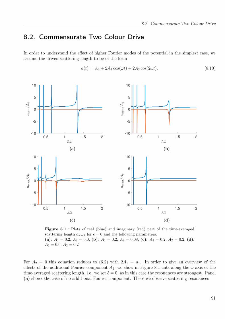
8.2. Commensurate Two Colour Drive
8.2. Commensurate Two Colour Drive
In order to understand the effect of higher Fourier modes of the potential in the simplest case, weassume the driven scattering length to be of the form
a(t) = A0 + 2A1 cos(ωt) + 2A2 cos(2ωt). (8.10)
0.5 1 1.5 2
-10
-5
0
5
10
(a)
0.5 1 1.5 2
-10
-5
0
5
10
(b)
0.5 1 1.5 2
-10
-5
0
5
10
(c)
0.5 1 1.5 2
-10
-5
0
5
10
(d)
Figure 8.1.: Plots of real (blue) and imaginary (red) part of the time-averagedscattering length ascatt for ε = 0 and the following parameters:(a): A1 = 0.2, A2 = 0.0, (b): A1 = 0.2, A2 = 0.08, (c): A1 = 0.2, A2 = 0.2, (d):A1 = 0.0, A2 = 0.2
For A2 = 0 this equation reduces to (6.2) with 2A1 = a1. In order to give an overview of theeffects of the additional Fourier component A2, we show in Figure 8.1 cuts along the ω-axis of thetime-averaged scattering length, i.e. we set ε = 0, as in this case the resonances are strongest. Panel(a) shows the case of no additional Fourier component. There we observe scattering resonances
91

8. Influence of Higher Fourier Modes of the Driven Potential
0 0.2 0.4 0.6 0.80.9
0.92
0.94
0.96
0.98
1
(a)
0 0.2 0.4 0.6 0.8
0.1
0.2
0.3
0.4
(b)
0 0.2 0.4 0.6 0.81
1.1
1.2
1.3
1.4
(c)
0 0.2 0.4 0.6 0.80
0.02
0.04
0.06
0.08
0.1
(d)
Figure 8.2.: Plots of the following fitting parameters for A1 = 0.05 in blue, A1 = 0.1in red and A1 = 0.2 in yellow:(a): Coefficient of determination R2 of the corresponding fitting procedure colouredfor different A1. (b): Imaginary part γ coloured for different A1, 1/max |Im ascatt|with black dashed line. (c): Resonant frequency ~ω0 coloured for different A1, ~ωside
with black dashed line, position of maximal imaginary part with black dotted line,(d): Width of the resonance δ coloured for different A1.
with a large enhancement of the real part of the scattering amplitude, while the imaginary part iszero except of non-shown delta-peaks exactly at the resonance positions. In Panel (b) we switchon the Fourier component A2 slightly and observe a non-vanishing imaginary part in the vicinityof all scattering resonances. This effect is strongest for the resonance with largest frequency, alsothe maximal real part is finite in this case. Panel (c) shows the case where A1 and A2 are equal.Here, this effect is stronger and involves a lower maximal real part for multiple resonances. Thiseffect is enhanced only at every second resonance. Panel (d) shows the case for A1 = 0, where onlyhalf of the resonances occur. This has been expected, as it should be recovered with the methodsof Chapter 6 while driving with the double driving frequency. As a non-vanishing imaginary part of
92

8.2. Commensurate Two Colour Drive
-0.2 -0.1 0 0.1 0.2
(hω − hω0)/δ
-2
0
2
4
logascatt
(a)
-0.2 -0.1 0 0.1 0.2
(hω − hω0)/δ
-2
0
2
4
logascatt
(b)
Figure 8.3.: Decade logarithm of modulus of real (blue) and imaginary (red) partof equation (8.11) for the parameters aBG = 1, γ = 10−2 (a) and aBG = 1, γ = 10−4
(b). The yellow curve in both panels shows the quantity log(|Re ascatt/Im ascatt|).
the scattering length ascatt is associated with particle loss, its occurrence limits the applicability ofour method. In order to obtain a strong enhancement of elastic scattering without strong particleloss, one has to tune the frequency on the flank of the resonance, where the real part is much largerthan the imaginary.
In the following we give a more quantitative insight in the dependency of the resonance with largestfrequency on the Fourier component A2. As the time-averaged scattering length ascatt looks in thepresence of higher Fourier components of the potential similar to (7.54), we fit the numerical datato the following approximate formula
1
ascatt(ω)=
1
aBG
ω − ω0
ω − ω0 − δ/~+ iγ. (8.11)
Figure 8.2 shows the dependency of the fitting parameters on the Fourier component A2. As it isshown in Panel (a), this fit works well for small values of A2, while for higher A2 the lowering of thecoefficient of determination R2 indicates a lower conformity of equation (7.54) and the numericaldata. We only considered data with a coefficient of determination larger than R2 ≥ 0.915. In Panel(b) the imaginary part γ is shown. As expected it vanishes for small A2 and reproduces the findingsin Chapter 7. With increasing A1 also γ increases following a power-law behaviour
γ = a
(A2
A1
)b
. (8.12)
As the imaginary part of the scattering length ascatt can be related by (5.68) to inelastic scattering,the occurrence of higher harmonics in the driving scheme leads to a lossy driving induced resonance.These losses occur, as for A2 6= 0 the side systems is no more decoupled from the open channels and
93

8. Influence of Higher Fourier Modes of the Driven Potential
therefore no bound state in the continuum occurs. Instead higher Floquet channels obtain a non-vanishing occupation leading to inelastic scattering. In Figure 8.3 we display the decade logarithm ofreal and imaginary part of equation (8.11) and see that in the vicinity of a resonance the imaginaryis larger than the real part. The yellow curve shows the quantity log(|Re ascatt/Im ascatt|) which hasa minimum exactly at resonance position. In order to get a large real part with a relatively smallimaginary part, one has to tune the driving frequency on the flank of the resonance, and, as thecomparison between Figure 8.3 (a) and (b) shows, lower the parameter γ. In Figure 8.2 (b) weshow in a black dashed line the quantity 1/max |Im ascatt|, which should equal γ in the ideal case.Indeed, we get a good agreement of both quantities verifying the correctness of the fitting procedure.Figure 8.2 (c) shows, that the change of A2 also changes the resonant frequency slightly comparedto A2 = 0. The black dashed lines are calculated by evaluating the eigenenergies of the side systemwhile assuming condition (7.18). We generalised the calculation presented in Section 7.3 to the casewhere A2 is non-zero by introducing next-nearest neighbour coupling A2 of the side systems channelswhile assuming that the coupling to the open channels completely vanishes. Although both linesposses similar qualitative behaviour, they deviate from each other especially in the case of largeA2. This deviation can shows that the assumption of an uncoupled side system is not true in thiscase. The non-vanishing next-nearest neighbour coupling of closed and open channels by A2 leadsin the sense of equation (3.8) to a shift of the resonance position. The black dotted lines show thefrequency position of maximal enhanced scattering and it fits well to the data obtained by the fittingprocedure. Figure 8.2 (d) shows that the width δ of the resonances lower with increasing A1.
We saw by this investigation that position and width of the scattering resonances are altered bythe value of A2. But most important is that a non-vanishing A2 implies a finite maximal scatteringlength, which is manifested at zero energy ε = 0 by a non-vanishing width γ. This findings areimportant for the discussion in the next Section.
8.3. Periodically Driven Magnetic Feshbach Resonance
In this Section we consider the case of a periodically driven magnetic Feshbach resonance. Asintroduced in the beginning of this Chapter we consider a contact potential with a time-periodicscattering length following equation (8.2). Its Fourier components are defined by
An =1
T
T∫0
dteinωt(
1− ∆
B2 cos(ωt) +B1 −B0
). (8.13)
This integral can be mapped by the substitution z = eisign(n)ωt to a line integral on the complex unitsphere. Using the residue theorem and assuming B2 < |B1 −B0| equation (8.13) is evaluated to
An = abg
δn,0 − ∆
(B1 −B0)√
12 − y2
[√1− y2 − 1
y
]|n| , (8.14)
94

8.3. Periodically Driven Magnetic Feshbach Resonance
0 0.1 0.2 0.3 0.4 0.5
B2 in units of |B1 −B0|
1
1.1
1.2
1.3
1.4
hω
(a)
0 0.1 0.2 0.3 0.4
B2 in units of |B1 −B0|
0
0.02
0.04
0.06
0.08
δin
unitsofE
D
(b)
0 0.1 0.2 0.3 0.4
B2 in units of |B1 −B0|
2
2.5
3
3.5
4
logmaxReascattin
unitsofA
0
(c)
Figure 8.4.: (a): Plot of position and width (dashed lines) of the driven magneticFeshbach resonance in dependency of the ac-magnetic field B2. In blue the results,where the maximal considered Fourier component of the potential is m1 = 10, areshown, while in red we consider m1 = 1. (b): Dependency of the width δ ofthe resonance on the ac-magnetic field B2 (c): Maximal enhancement of elasticscattering maxRe ascatt = 1
2γ over the ac-magnetic field B2. All plots have beendone with ∆ = −2(B1 −B0), while B1 −B0 < 0.
while we introducedy =
B2
B1 −B0
. (8.15)
Its structure reveals that An drops polynomially with increasing Fourier index n in the case of|y| < 1 and the truncation method defined in Section 8.1 is applicable in this case. As a result weplot in Panel (a) of Figure 8.4 in blue position and width of the resonance with largest frequencyover the strength of the ac-magnetic field B2. It can be seen that both resonance position and
95

8. Influence of Higher Fourier Modes of the Driven Potential
width grow with the strength of the ac-magnetic field B2. This is also the case for the results ofa calculation considering only one Fourier mode and can thus be explained qualitatively with thefindings of Subsection 7.5.2. The differences of both results can be understood by the results ofSection 8.2, as the higher Fourier components increase with larger y. In Panel (c) we show that themaximal enhancement of the real part of the time-averaged scattering amplitude decreases with theac-magnetic field B2. It is infinite if only one Fourier channel of the potential is considered. In theconsideration of higher harmonics it becomes infinitely large only in the case of B2 = 0, while thewidth vanishes at B2 = 0. This effect might be important for experiments, where a large width and alarge enhancement of scattering are favourable. We see in Figure 8.4 that the maximal enhancementof scattering decreases with the ac-magnetic field B2, while the width increases. Therefore in practiceone has to do a trade-off between both quantities and might chose a value of B2, which allows anotable enhancement of scattering while the width is not too small.
8.4. Frequency and Length Scale for Scattering of UltracoldAtoms
At the end of this Chapter we give an overview of the frequency and length scales occurring ina driven magnetic Feshbach resonance in the case of bosonic 85Rb and 133Cs atoms. For 85Rb wespecialise on the resonance at B0 = 155.04 G with the width ∆ = 10.7 G and a background scatteringlength of abg = −443 aBohr [102]. For 133Cs we consider the resonance with B0 = 547 G, ∆ = 7.5 Gand abg = 2500 abohr [38]. As all of these resonances are so-called entrance channel dominated [38],the contact potential is a valid approximation of the actual inter-atomic interaction over a widerange of magnetic fields within the width of the magnetic Feshbach resonance. The frequency scaleof the driving induced scattering resonance, as displayed in Figure 8.4 (a), is given by the dimerenergy divided by ~, while the length scale is given by the zeroth Fourier component A0 of the drivencontact potential. Therefore Figure 8.5 can be used in order to convert the dimensionless y-axis ofFigure 8.4 into physical units in order to estimate the value of the frequency or the field strength,which has to be applied in order to investigate the scattering resonances. In Figure 8.5 we calculatethe dimer energy by
ED =~2
2µ
1
[A0(B2 = 0)]2, (8.16)
where µ denotes the reduced mass and A0(B2 = 0) is calculated with equation (8.14). Panel (a)of Figure 8.5 shows that the dimer energy of the considered Rb resonance lies in the MHz rangeand increases if |B1 − B0| increases. Due to equation (6.5) the results are only valid for drivingfrequencies below the energy scale of the potential, which is for 85Rb given by the van der Waalsenergy EvdW ≈ 6 MHz [38]. This is indicated in Figure 8.5 by the red dashed line and reveals thatthis approximation is only valid for small deviations of B1 from B0. In combination with Figure 8.4(b) this shows that the width of the resonance lies in the regime of 100 kHz. For 133Cs the situa-
96

8.4. Frequency and Length Scale for Scattering of Ultracold Atoms
0 2 4 6 8B1 −B0 in units of ∆
1
2
3
4
5
6
ED/h
inMHz
(a)
-6 -4 -2 0B1 −B0 in units of ∆
1
2
3
4
5
6
ED/h
inkHz
(b)
0 2 4 6 8
B1 −B0 in units of ∆
103
104
105
A0in
unitsofaBohr
(c)
-6 -4 -2 0
B1 −B0 in units of ∆
104
105
106
A0in
unitsofaBohr
(d)
Figure 8.5.: (a): Plot of the dimer energy ED (blue line) and the van der Waalsenergy scale (dashed red line) for 85Rb(b): Plot of the dimer energy ED for 133Cs(c): Plot of A0(B2 = 0) in Bohr radii aBohr for 85Rb(b): Plot of A0(B2 = 0) in Bohr radii aBohr for 133Cs
tion is different, as the dimer energy lies in the kHz regime and thus way below the van der Waalsenergy of EvdW = 2.666 MHz [38]. The width of the resonance is of the order of 100 Hz. Panel(c) and (d) can be used to express the maximal enhancement of scattering shown in Figure 8.4 (c)in Bohr radii. In order to validate the approximation of ε = 0, the dimer energy has to be largerthan the temperature of the Bose-Einstein condensate. Assuming a temperature of T ≈ 10−9 nK,we arrive at a frequency scale of 100 Hz. If this condition is not fulfilled, the maximal enhancementof elastic scattering is lower due to the finite energy ε as discussed in Subsection 7.5.1.
97


9. Conclusion and Outlook
In Section 9.1 we summarise the most important findings of our work and give concluding remarks,while Section 9.2 is dedicated to the Outlook.
9.1. Conclusion
The tuning of the interaction strength enables a rich amount of experimental settings, especiallyin the case of ultracold quantum gases [1, 2, 38]. Due to low kinetic energies s-wave scattering isdominant and the interaction strength can be described by a single parameter, named scatteringlength. Magnetic Feshbach resonances provide a common tool of controlling the scattering lengthexperimentally. A limiting factor of their application is that they occur only at certain characteristicmagnetic field strengths. Recent works [3–5] showed that periodic driving can enhance the scatteringof quantum particles in a dramatic way, opening new possibilities of controlling the scattering length.
This thesis investigated the two-body problem with a time-periodic interaction potential. Basedon Floquet theory the Floquet-partial wave expansion was derived in Chapter 5 as a generalisationof scattering theory which is able to deal with time-periodic interaction potentials. It was used tocalculate time-averaged scattering amplitudes, cross sections and Floquet states.
We applied in Chapter 6 the Floquet-partial wave expansion to a sinusoidally driven contact po-tential, which describes the two-body interactions of quantum particles in the regime of s-wavescattering. Due to the simple structure of the potential the time-dependent scattering problem(6.11) was mapped to the recursion relation (6.37), which connects different Fourier-components ofits steady-state wave function. The solution of the recursion was used to calculate the time-averagedscattering amplitude. Although this recursion is non-linear in the Fourier index, it can be solvednumerically for arbitrary driving frequencies. In addition we found an analytic solution for highand low driving frequencies. At low frequencies the resulting Floquet state follows adiabatically thetime-evolution of the driven potential.
The main result of our investigation, displayed in Chapter 7, concerned the observation of drivinginduced scattering resonances, which occur along lines in the parameter space of driving strength andfrequency. In the vicinity of these resonances scattering is dramatically enhanced, which allows thetuning of the time-averaged scattering amplitude to large positive or negative values. The width ofthese resonances can be adapted by the driving strength, while the enhancement is controlled by the
99

9. Conclusion and Outlook
driving frequency. It turned out that they are lossless, as no inelastic scattering due to absorptionof energy quanta from the drive field is present in their vicinity.
The occurrence of these scattering resonances was related to the emergence of bound states in thecontinuum and explained in Section 7.2 as Fano-Feshbach resonances involving these bound stateslocated in a Floquet side-band. With this finding we were able to calculate the resonance positionfor arbitrary driving strength and frequency. For weak driving a resonance occurs, if the frequencymatches with a transition between the scattering state and the universal dimer state of the contactpotential. We spotted that these resonances only emerge if the driving frequency is larger than theparticle energy divided by ~.
The time-averaged scattering amplitude can be approximately described by simple formulas (7.43)and (7.54), where equation (7.54) was derived in Section 7.4.2 from scattering by a two-channel modeland approximates the numerical data slightly better than (7.43). These formulas were used in Sec-tion 7.5 in order to extract position and width of scattering resonances for almost arbitrary drivingstrengths. Their width increases with the driving strength and vanishes in the limit of small driv-ing. In addition we found in Section 7.6 a Kramers-Kronig like relation between real and imaginarypart of the time-averaged scattering amplitude, which is also fulfilled by the approximative formulas.
A possible experimental realisation of this theory is the periodically driven magnetic Feshbach res-onance [3]. In order to describe this setting with a better accuracy, the scattering by a contactpotential with a more general time-periodic driving was investigated in Chapter 8. In this caseinelastic scattering is present in the vicinity of the resonance, but by tuning the frequency slightlyaway from it, elastic scattering can be still enhanced without suffering a large amount of losses. Wewere able to calculate position and width of the periodically driven magnetic Feshbach resonance ina wide range of driving strengths.
In summary we conclude that it is possible to tune the scattering length and therefore the in-teraction strength of particles by periodic driving. This driving induced scattering resonance hasthe benefit of being almost lossless and tunable solely by the driving parameters. This allows alarger experimental flexibility, as unlike in the case of a magnetic Feshbach resonance the magneticfield strength can be set relative far away from the resonance without loosing the enhancement ofscattering. In comparison to an optical Feshbach resonance it has the advantage of being almostlossless. In addition, it might be applied to tune the interaction in ultracold gas experiments, whereno magnetic or optical Feshbach resonance is available.
9.2. Outlook
Although the contact potential is a simple model of the more complicated inter-atomic interactionpotential, its study in a driven case is highly non-trivial. Despite the fact that a quite general formof the solution is given in this thesis, several points remain unsolved.
100

9.2. Outlook
At first we want to mention, that it would be of large interest, if also in the case of a periodi-cally driven scattering resonance general formulas for calculating position and width like equations(3.8) and (3.9), which are applicable for magnetic Feshbach resonances, exist. Such formulas wouldgive a clear definition and allow a calculation of these quantities without relying on a fitting proce-dure or being restricted to approximative solutions.
Secondly, a detailed study of the case, where the driving amplitude a1 extends the value of thetime-averaged one, has not been done. It would be of interest, as it can be reached in experimen-tal setups [2]. Our investigations revealed that scattering resonances only exist in the case of apositive scattering length of the contact interaction, as their emergence is connected with the ex-istence of a bound dimer state. In the case of a1 > a this dimer state is only present in a part ofthe driving period. Therefore it would be interesting, if the occurrence of scattering resonances isalso possible in this case or if the partial absence of the bound state destroys the possibility of thesystem to enhance elastic scattering. In order to do this investigation it would be advantageous tofind a formalism, where 1/a is treated as a smallness parameter or use a different scattering potential.
We only dealed with two body physics, but experimental realisations of Feshbach resonances arealso limited by losses due to three-body collisions. Due to their experimental relevance and basedon [4] it would be interesting to investigate the occurrence of three body losses in the case of a pe-riodically driven inter-particle interaction. Also the investigation of higher partial waves in Floquetscattering would be interesting.
A natural extension of the findings of Chapter 8 would be the investigation of more sophisticateddriving schemes. This includes the case of applying a general time-periodic driving, like a sawtooth,on a periodically driven magnetic Feshbach resonance. A more complicated setting would includethe driving of the system with two incommensurate frequencies.
As we observed driving induced scattering resonances by using the methods of theoretical physics,an interesting next step would be implementation of these resonances in an experimental setup. Inthe following we discuss two possible fields of application for driving induced Feshbach resonancesand give an introduction in wave-guide arrays, where Floquet physics can be made visible directly.
9.2.1. Periodically Driven Optical Feshbach Resonance
Optical Feshbach resonances are induced by laser light, which is near resonant to a transition be-tween a scattering state and a molecular bound state. As the bound state is usually not a groundstate, it decays spontaneously. This decay limits the applicability of the optical Feshbach resonance,as it results in strong losses in its vicinity. As shown in Figure 9.1, there are processes which leadto a limited amount of elastic scattering, as the shift of the scattering length is proportional to thedisplayed interaction shift, which can be enhanced up to 30%. In order to get a larger enhancementof elastic scattering we suggest to apply the driving induced Feshbach resonance in this setting. Afeasible protocol would locate the bias of the periodic drive at the side of the optical Feshbach reso-nance, where the losses are negligible, but the rate of elastic scattering can be changed noticeably.
101

9. Conclusion and Outlook
Figure 9.1.: Plot of an optical Feshbach resonance in ultra long-range Rydbergmolecules. Blue dots represent the interaction shift over the detuning of the laser,which created the optical Feshbach resonance. The orange curve has been calculatedusing an approximate theoretical model. The purple curves are ion signals used formeasuring the resonance structure. The Figure was created by Thomas et al. [69],where a detailed explanation of the emerging quantities is found.
In this region it could be possible to enhance the scattering amplitude without suffering a largeamount of losses. The question is, if it is possible to minimise both losses from the optical Feshbachresonance and the driving induced one in such a way that the method is applicable. Equation (3.14)suggests that driving scheme can be implemented by either altering the intensity or the detuning ofthe laser used for creating the optical Feshbach resonance periodically.
This possible implementation of the driving induced Feshbach resonance is also of theoretical in-terest, as it combines the field of periodic driving with the investigation of dissipative systems. Inorder to deal with it correctly, losses have to be included in the formalism. A straight-forward way ofobtaining this theoretically is the extension of Floquet-scattering theory to non-hermitian potentials.The investigation of scattering by a non-hermitian potential in an one-dimensional tight-bindingchain [103] revealed fascinating results as the complete invisibility of the potential in scattering con-figurations. This effect brings up the question, how dissipation can change or even suppress resonantfeatures and therefore dramatically redraft the behaviour of the driven system. As the simplest non-trivial scattering potential we suggest the contact interaction with a complex scattering length. Asecond compelling and very general approach would be the scattering by a square well potential witha complex potential strength. As in the case of a driven hermitian square well potential there existsa solution in a closed form [80], it is the hope that this might be extended to a driven-dissipativecase in an intuitive manner.
102

9.2. Outlook
9.2.2. Scattering in Quantum Gases with Internal Degree of Freedom
The development of the optical dipole trap [104] enabled to trap Bose-Einstein condensates in dif-ferent hyperfine states and therefore with a spin-like internal degree of freedom. These spinorBose-Einstein condensates possess a rich phase diagram especially in the presence of an externalmagnetic field [105]. For example, by changing the magnetic field across a critical value, one isable to observe a quantum phase transition to a ferromagnetic phase [106]. Magnetic Feshbachresonances are limited for the control of the interaction strength in these systems, as they cannotbe tuned independently from the magnetic field and only occur at restricted field strengths. Thedriving induced scattering resonance can be induced in a wide range of magnetic field strengthsand the enhancement of scattering is controlled by use of the driving frequency and strength. Itwould allow the enhancement of scattering while simultaneously tuning the magnetic properties ofthe spinor gas by changing the magnetic field.
One specific example, on which the driving induced scattering resonance can be applied, is thecontrol of scattering rates of spin impurities with a bath. In a recent experiment [107] impuritiesof neutral 133Cs atoms with total internal angular momentum of Fi = 3 are immersed into a Bose-Einstein condensate of 87Rb atoms with Fb = 1 and are used to probe properties of the condensate.For example it is possible to detect the hyperfine-Zeeman level of the condensate by investigatingspin-exchange dynamics between impurity and bath. Additionally, this setup enables the observationof coherent dynamics by preparing the impurity in a quantum superposition state. The de-phasingof the dynamics is influenced by the actual value of the elastic scattering length. Theoretical andexperimental investigations indicate the presence of a magnetic Feshbach resonance [108], which al-lows to enhance both elastic and spin-exchange scattering rates for collisions between impurity andbath. In practice the scattering can only be enhanced for collisions in one Zeeman level, because theresonances for different levels are located at different magnetic field strengths.
This restriction can be overcome by the application of the driving induced scattering resonance [108].If possible, one has to choose a bias magnetic field B1 in a region, where all magnetic resonances pro-vide a positive scattering length. By applying a sinusoidally modulated magnetic field with strengthB2 one would be able to create a driving induced scattering resonance in all Zeeman levels simul-taneously. This would enhance scattering in total and fasten up the interaction process betweenimpurity and bath, which would be a benefit in investigations probing the Bose-Einstein condensatein a non-equilibrium state.
In order to model the situation in a better way, the spin-like internal degree of freedom has tobe included in the interaction potential. The most basic way to do this is to use the contact po-tential as spatial degree of freedom and add an internal matrix structure, which couples differentchannels of the wave function [105, 109]. This can be expressed using the spin operators of thescatterers [109]. It would be interesting to observe how this additional degree of freedom and thematrix structure of the potential is able to alter the properties of scattering resonances or if it caneven be used in order to create new ones. Another direction would be the investigation, if periodicdriving can be used in order to control collisions with a spin-exchange efficiently. This would makeit possible to prepare or conserve a favoured hyperfine state in a system, which is interacting with
103

9. Conclusion and Outlook
its environment.
9.2.3. Driven Impurities in Coupled Wave-Guide Arrays
Another path of further research goes back to one-dimensional systems with periodically drivenimpurities. A profound experimental setup for investigating single particle dynamics in those systemsare dielectric [110, 111] and plasmonic [112] wave-guide arrays. The paraxial Helmholtz equation[110]
i∂
∂zψ(x, y, z) = − 1
2kwg
[∂2
∂x2+
∂2
∂y2+ V (x, y)
]ψ(x, y, z) (9.1)
describes the propagation of light in these wave-guides and is mathematically equivalent to theSchrödinger equation [113]. Therefore the behaviour of light can be used in order to mimic quantummechanics. As it can be seen in equation (9.1), time in quantum mechanics corresponds to thepropagation direction of light in the wave-guides, which is here considered as z-direction, the massis given by the wave vector in the wave-guide kwg and the wave function ψ is given by the light field.A non-vanishing potential can be induced by tuning the refractive index.
If the wave-guides are arranged in a lattice in x or y direction, the dynamics of light in such anarray is governed by a lattice Hamiltonian similar to the tight-binding model [114]. The hoppingconstant J in this case is determined by the overlap of the evanescent light-modes in the wave-guides.Figure 9.2 sketches a possible experimental setup, which consists of a tight-binding model with aperiodically modulated site.
As wave-guide arrays are accessible and allow tuning of parameters, they are suitable for the in-vestigation of defect states [110] and the realisation of topological models. A recently created ex-perimental setup [115] deals with the stability of topological protected edge states under periodicmodulation. The experimental situation is modelled by two one-dimensional Su-Schrieffer-Heegerchains [116], which are coupled via a central site acting as an impurity. A sketch of this setting isdone in Figure 9.3.
The Su-Schrieffer-Heeger model consist of a chain with staggered hopping amplitudes and as a modelwith a non-trivial topology it possesses topological protected edge states. A band structure of theexperimentally realised Hamiltonian is shown in Figure 9.4. It consists of two bulk bands related tostates with finite momentum and a bound edge state emerging at the central site.
In order to probe the robustness of the system against local perturbations, the position of thewave-guide corresponding to the central site is periodically modulated perpendicular or parallel tothe direction of the SSH-chain. As the distance to the neighbouring lattice sites is modulated peri-odically, this results in a periodically modulated hopping amplitude to and from the impurity site.The curvature of the wave-guide can be related to a time-dependent on-site potential [115]. Asan initial condition light is only located in this impurity site. The question is, if the edge state re-mains localised in the presence of periodic modulation or if a transition to the bulk band is occurring.
104

9.2. Outlook
Figure 9.2.: Possible experimental setup of dielectric wave-guide arrays realising anone dimensional tight-binding model. All arrays are oriented in z-direction, whichcorresponds to the time in quantum mechanics, while the lattice is formed in x-direction. As an impurity one wave-guide is periodically modulated perpendicularto the direction of the lattice, inducing a time-dependend term in the tight-bindingmodel. The picture was created by C. Jörg [115].
In order to complement the experimental results [117], the corresponding time-periodic Schrödingerequation is solved using Floquet theory. The full time-evolution of the system at arbitrary drivingstrength can be determined by diagonalising the Floquet Hamiltonian (4.10), which yields Floquetmodes and energies. With Floquet theory we can calculate the probability, that a state with mo-mentum k and energy E is occupied.
In addition it would be intriguing to invert the setting by looking at scattering by the driven im-purity in a model with a topological background and investigate the influence of the periodicallymodulated hopping amplitude on the scattering process. A goal of this research direction would beto find a relation between the excitation of the defect state and the transmission amplitude throughthe driven barrier.
105

9. Conclusion and Outlook
Figure 9.3.: Sketch of the theoretical model being realised in experiment. It consistsof two SSH chains, which have staggered hopping amplitudes J1 and J2, and areconnected by the impurity site. The hopping J(t) to and from the impurity isperiodically modulated.
-1 -0.5 0 0.5 1
k/π
-1.5
-1
-0.5
0
0.5
1
1.5
energy
inA.U
.
Figure 9.4.: Band structure of the SSH model. In blue the dispersion of the bulkbands is drawn, while the energy of the defect state is visualised as a straight lineat an energy of zero.
106

A. Contact Potential
The idea of the contact potential, also named pseudo potential, is to approximate a complicatedpotential by a simple one. This approximation is valid in the case of scattering with low energies,where the de-Broglie wavelength is much larger than the range of the actual potential and thepotential is effectively present only in the origin. This idea has been discussed in literature of earlierdays of quantum mechanics [118,119] and considered as a simplification of the scattering by a hard-sphere potential. We present a derivation in the case of s-wave scattering [55]. Starting point is thewave function solving the scattering by a hard-sphere potential
R0(r) = A0[j0(kr)− tan(δ0)y0(kr)], (A.1)
which has been introduced in Section 2.3. As the contact potential is designed to act on the wavefunction only in the origin, we extend equation (A.1) to be also valid inside the hard sphere andintegrate the radial Schrödinger equation (2.9) over a sphere of radius r0 around the origin usingGauss theorem ∫
Br0 (0)
d3r[∆ + k2]R0(r) =
∫∂Br0 (0)
dA∇R0(r0) +
∫Br0 (0)
d3r k2R0(r) (A.2)
In the limit of r0 → 0 the last term vanishes, while the first is evaluated by using dA = dΩr20er and
∇R0(r0) · er = ∂rR0(r)∣∣r=r0
to −4πk
tan(δ0)A0. The amplitude A0 can be rewritten as the operatorlimr→0
∂∂rrR0(r), if R0(r) is of the Form (A.1). The identity 1 =
∫d3rδ3(r) is used in order to drop
the integral
[∆ + k2 +4π
k cot(δ0)δ3(r)
∂
∂rr]R0(r) = 0. (A.3)
If equation (A.3) is compared to the radial Schrödinger equation, the contact potential can beidentified to
Vcontact(r) =−2π~2
µk cot(δ0)δ3(r)
∂
∂rr, (A.4)
with µ as the reduced mass. For the case of scattering with low energies the scattering length a(2.20) can be used to further simplify the potential to
Vcontact(r) =2π~2a
µδ3(r)
∂
∂rr. (A.5)
In the following we discuss some properties of the contact potential: At first, the difference to a
107

A. Contact Potential
bare delta-function potential is made clear. Therefore the wave function is expressed by a Laurentseries
R(r) =∞∑
n=−∞
cnrn. (A.6)
The evaluation of the delta function integral, using equation (6.6), leads to the result∫ ∞0
drδ(r)R(r) =c0
2+
1
2
−1∑n=−∞
cnrn∣∣r=0︸ ︷︷ ︸
divergent terms
. (A.7)
The divergent terms only disappear, if the coefficients cn vanish for all n ≤ −1. The same calculationis also done in the case of the contact potential∫ ∞
−∞drδ(r)
∂
∂r[rR(r)] =
∫ ∞−∞
drδ(r)∞∑
n=−∞
cn(n+ 1)rn =c0
2+
1
2
−2∑n=−∞
cnrn∣∣r=0︸ ︷︷ ︸
divergent terms
. (A.8)
If there are no divergent terms in the test function, the result of both calculations is the same. Butif only divergent terms of the order 1
rare present, they will not appear in the contact potential
calculation, but in the one using the delta function. This vanishing of divergences is necessary inorder to obtain useful scattering properties in case of s-wave scattering by a short range interaction,as the ansatz functions (6.12) posses an 1/r divergence in the origin.
A.1. Scattering by a Contact Potential
In the following we derive the scattering properties of the pseudo potential by assuming a scatteringstate of the form
R0(r) =sin(kr)
kr+ f
eikr
r(A.9)
and using the formalism introduced above. The first part of (A.9) is the s-wave part of the planewave, the second the scattered spherical wave. Equation (A.9) solves the free radial Schrödingerequation for each r 6= 0. In order to evaluate the Dirac delta-function, an integration on a sphere ofradius r0 around the origin similar to (A.2) is done∫
Br0 (0)
dΩdr r2[∆R0(r) + k2R0(r)] + 4πaδ3(r)[∂
∂rrR0(r)] (A.10)
Inserting (A.9) into (A.10) yields the equation −f − a(1 + ikf) = 0. From this the scatteringamplitude f can be derived to
f =−1
1a
+ ik. (A.11)
108

A.2. Bound State
A.2. Bound State
At last, we mention that the contact potential possesses a bound state in the case of positivescattering length a. This can be found out by solving the Schrödinger equation[
∆− 4πaδ3(r)∂
∂rr
]ψ(r) =
2m
~2Eψ(r) (A.12)
with the ansatzψ(r) = Ce−κ|r|. (A.13)
Similar to (A.10) an integration around the origin leads to the result κ = 1a, which inserted into
equation (A.12) for r 6= 0 yields the bound state energy of E = −ED. Here we introduced the dimerenergy
ED =~2
2µ
1
a2. (A.14)
We followed [3] and named this bound state energy dimer energy, as its wave function correspondsto a bound dimer state.
109

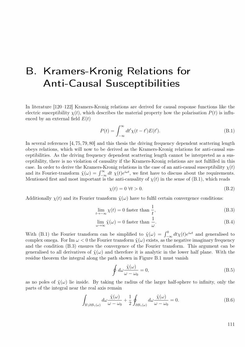
B. Kramers-Kronig Relations forAnti-Causal Susceptibilities
In literature [120–122] Kramers-Kronig relations are derived for causal response functions like theelectric susceptibility χ(t), which describes the material property how the polarisation P (t) is influ-enced by an external field E(t)
P (t) =
∫ ∞−∞
dt′χ(t− t′)E(t′). (B.1)
In several references [4, 75, 79, 80] and this thesis the driving frequency dependent scattering lengthobeys relations, which will now to be derived as the Kramers-Kronig relations for anti-causal sus-ceptibilities. As the driving frequency dependent scattering length cannot be interpreted as a sus-ceptibility, there is no violation of causality if the Kramers-Kronig relations are not fulfilled in thiscase. In order to derive the Kramers-Kronig relations in the case of an anti-causal susceptibility χ(t)and its Fourier-transform χ(ω) =
∫∞−∞ dt χ(t)eiωt, we first have to discuss about the requirements.
Mentioned first and most important is the anti-causality of χ(t) in the sense of (B.1), which reads
χ(t) = 0 ∀t > 0. (B.2)
Additionally χ(t) and its Fourier transform χ(ω) have to fulfil certain convergence conditions:
limt→−∞
χ(t) = 0 faster than1
t, (B.3)
limω→∞
χ(ω) = 0 faster than1
ω. (B.4)
With (B.1) the Fourier transform can be simplified to χ(ω) =∫ 0
−∞ dtχ(t)eiωt and generalised tocomplex omega. For Im ω < 0 the Fourier transform χ(ω) exists, as the negative imaginary frequencyand the condition (B.3) ensures the convergence of the Fourier transform. This argument can begeneralised to all derivatives of χ(ω) and therefore it is analytic in the lower half plane. With theresidue theorem the integral along the path shown in Figure B.1 must vanish∮
dωχ(ω)
ω − ω0
= 0, (B.5)
as no poles of χ(ω) lie inside. By taking the radius of the larger half-sphere to infinity, only theparts of the integral near the real axis remain∫
R\∂Bγ(ω)
dωχ(ω)
ω − ω0
+1
2
∮∂Bγ(ω)
dωχ(ω)
ω − ω0
= 0. (B.6)
111
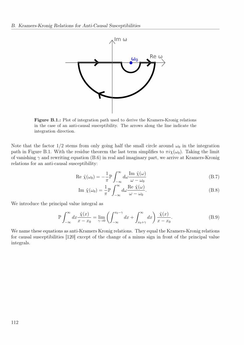
B. Kramers-Kronig Relations for Anti-Causal Susceptibilities
Figure B.1.: Plot of integration path used to derive the Kramers-Kronig relationsin the case of an anti-causal susceptibility. The arrows along the line indicate theintegration direction.
Note that the factor 1/2 stems from only going half the small circle around ω0 in the integrationpath in Figure B.1. With the residue theorem the last term simplifies to πiχ(ω0). Taking the limitof vanishing γ and rewriting equation (B.6) in real and imaginary part, we arrive at Kramers-Kronigrelations for an anti-causal susceptibility:
Re χ(ω0) = − 1
πP∫ ∞−∞
dωIm χ(ω)
ω − ω0
(B.7)
Im χ(ω0) =1
πP∫ ∞−∞
dωRe χ(ω)
ω − ω0
. (B.8)
We introduce the principal value integral as
P∫ ∞−∞
dxχ(x)
x− x0
= limγ→0
(∫ x0−γ
−∞dx+
∫ ∞x0+γ
dx
)χ(x)
x− x0
. (B.9)
We name these equations as anti-Kramers Kronig relations. They equal the Kramers-Kronig relationsfor causal susceptibilities [120] except of the change of a minus sign in front of the principal valueintegrals.
112

C. Derivation of Scattering Amplitude ofa Simple Coupled-Channel Model
In this Appendix we calculate the scattering of a two-component wave function
ψ(r) =
(ψ0(r)ψ1(r)
)(C.1)
by the coupled-channel Hamilton operator (7.50). The radial Schrödinger equation H(r)ψ(r) =Eψ(r) for the coupled-channel scattering problem reads[
− 1
r2
∂
∂rr2 ∂
∂r+
2a0
r2δ(r)
∂
∂rr
]ψ0(r) +
2aWW
r2δ(r)
∂
∂rrψ1(r) = Eψ0(r), (C.2)[
− 1
r2
∂
∂rr2 ∂
∂r+
2a1
r2δ(r)
∂
∂rr + v
]ψ1(r) +
2aWW
r2δ(r)
∂
∂rrψ0(r) = Eψ1(r). (C.3)
We use as an ansatz
ψ0(r) = eikr∣∣s−wave
+ feikr
r=
sin(kr)
kr+ f
eikr
r(C.4)
in the open channel, which is considered to be channel zero, and
ψ1(r) = Ce−κr
r(C.5)
in the closed one. The quantity f denotes the s-wave scattering amplitude and C is the normalisationconstant of the closed channel wave function.
Inserting both ansatz-wave functions in the respective coupled-channel equations for r 6= 0, weobtain the dispersion relation
k2 = E (C.6)
for the free solution ψ0 andκ2 = v − k2 (C.7)
for the closed channel solution ψ1. We assume v to be positive and of a strength necessary in orderto make ψ1 a bound state, i.e. v > k2. In order to determine the constants C and f we multiplyboth equation (C.2) and (C.3) by r2 and integrate from 0 to a small radius εr similar to Section 6.At last, we take the limit of vanishing εr. Equation (C.2) can thus be rewritten as
(1 + ika0)f + a0 − aWWκC = 0. (C.8)
113

C. Derivation of Scattering Amplitude of a Simple Coupled-Channel Model
0.8 0.9 1 1.1 1.2V in units of 1/a21
-20
-15
-10
-5
0
5
10
15
20
fin
unitsofa1
0.8 0.9 1 1.1 1.2V in units of 1/a21
0
5
10
15
20
25
30
35
fin
unitsofa1
Figure C.1.: Plot of real (a) and imaginary (b) part of the scattering amplitudef for the case of aWW = 0.25a1 (blue) and aWW = 0.75a1 (red), E = 10−3/a2
1 anda0 = a1.
With the same argumentation equation (C.3) is simplified to
(1− a1κ)C + aWW(1 + ikf) = 0. (C.9)
These two equations are linear in f and C. The amplitude C is given by
C =aWW
a1κ− 1 + ik(a2WWκ+ a0a1κ− a0)
, (C.10)
while the scattering amplitude f can be written in the form
f =−1
1a
+ ik. (C.11)
Hereby we define the scattering length
a = a0
(1 +
a2WWκ/a0
1− a1κ
)(C.12)
depending on the coupling strength aWW and the offset potential v of the closed channel. The κdependence of equation (C.12) is similar to the magnetic field dependency of equation (3.12). Forκ = 1/a1 the scattering length diverges and leads to a resonantly enhanced scattering amplitude ofvalue f = i
k. This condition is equivalent to the equality of the energy of the scattered wave in the
first channel E and the energy of the bound state Ebound = V − 1a2
1in the second one. Figure C.1 shows
the dependence of the scattering amplitude on the offset potential v for different coupling strengthsaWW. The width of the resonance increases with growing coupling strength aWW. The shape of thescattering amplitude is similar to the results obtained in the case of the driven scattering problem ifone plots it over the driving frequency. Therefore it is suggestive to replace the offset potential v byan integer multiple of the driving frequency |n|~ω in order to get a formula to fit the two-channelmodel on the more complicated case of the driven scattering problem
114

− 1
f=
1
a0
1− a1
√|n|~ω − E
1− a1
√|n|~ω − E + a2
WW/a0
√|n|~ω − E
+ ik. (C.13)
This formula can be simplified near a resonant frequency ω0 fulfilling the resonance condition
E = − 1
a21
+ |n|~ω0. (C.14)
We approximate the square root by a linear expression
√|n|~ω − E =
√|n|~(ω − ω0) +
1
a21
≈ 1
a1
+a1|n|~
2(ω − ω0). (C.15)
In this case the inverse scattering amplitude can be brought to the form
− 1
f=
1
aBG
ω − ω0
ω − ω0 − δ/~+ iγ, (C.16)
where we have introduced by
aBG = a0
(1− a2
WW
a0a1
), (C.17)
the background scattering length, which determines the scattering amplitude in the case of aninfinitely large frequency ω. The width of the real part of the scattering amplitude corresponds to
δ =2a2
WW
a0a1|n|1
1− a2WW
a0a1
1
a21
. (C.18)
The quantity
γ = k (C.19)
characterises the width of the imaginary part and its inverse corresponds to the maximal value ofthe scattering amplitude. Although having a much simpler structure than (C.11), Figure C.2 showsthat the approximation (C.13) fits quite well to the correct value of (C.11). Formula (C.13) has beenreported recently by [80], but without the derivation above.
115
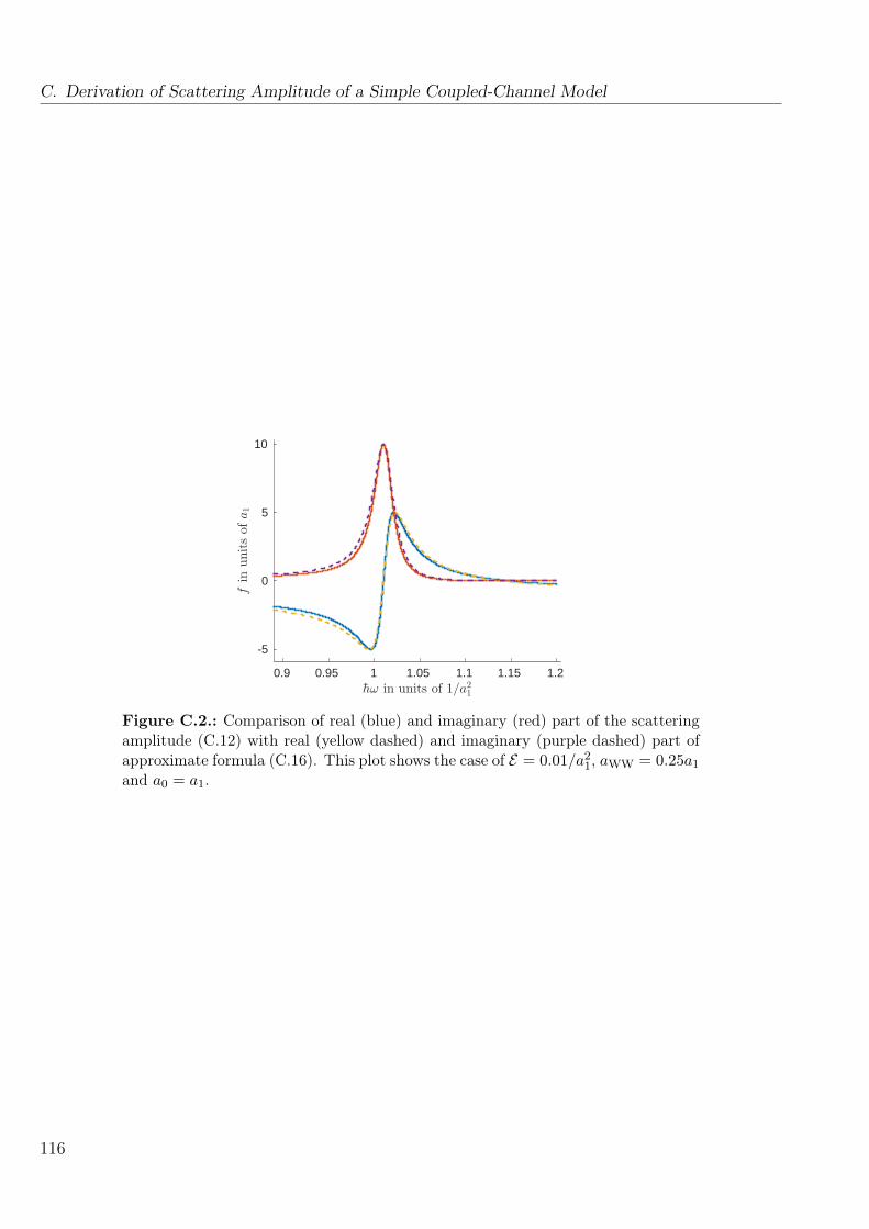
C. Derivation of Scattering Amplitude of a Simple Coupled-Channel Model
0.9 0.95 1 1.05 1.1 1.15 1.2hω in units of 1/a21
-5
0
5
10
fin
unitsofa1
Figure C.2.: Comparison of real (blue) and imaginary (red) part of the scatteringamplitude (C.12) with real (yellow dashed) and imaginary (purple dashed) part ofapproximate formula (C.16). This plot shows the case of E = 0.01/a2
1, aWW = 0.25a1
and a0 = a1.
116

D. Limit of Vanishing γ ofApproximative Formula (7.54)
In this Section we evaluate the limit of γ going to 0 of the formula (7.54). For the real part (7.63)the limit can be straight-forwardly evaluated to
− limγ→0
Re f = aBG
(1− δ
~ω − ~ω0
). (D.1)
This equals to the limit of Γ → 0 of equation (7.43), if we identify abg = aBG and ∆ = δ. Theimaginary part (7.64) converges in this limit to a Dirac-delta function, which is peaked at theresonance frequency ω0. This can be made clear by showing that the quantity −Im f(ω) fulfils theproperties of the delta distribution in this limit. These are [123]
δ(x) =
0, ∀x 6= 0
∞, x = 0(D.2)
and ∫ ∞−∞
dxδ(x) = 1. (D.3)
We start with (D.2) and let x = ω−ω0 be unequal to zero. Then the imaginary part of the scatteringamplitude evaluates to
Im f(ω) =γa2
BG(x− δ)2
γ2a2BG(x− δ)2 + x2
+γa2
BG
1 + γ2a2BG
. (D.4)
The last term equals Im f0(∞) and the whole imaginary part (D.4) vanishes in the limit γ → 0 ifω 6= ω0. For the case of ω = ω0 the imaginary part (D.4) equals 1/γ, which tends to infinity forvanishing γ.
The proof of condition (D.3) is a bit more involved, as it includes an integration over a non-trivialfunction. The integral
∫∞−∞ dω [−Im f(ω) + Im f(∞)] can be evaluated using partial integration
to ∫ ∞−∞
dω [−Im f(ω) + Im f(∞)]
= limR→∞
−a2BGγ
δ(−√c log [c(δ − x)2 + x2]− (c− 1) arctan
(c(x−δ)+x√
c δ
))√c (c+ 1)2
∣∣∣∣∣∣R
−R
= −aBGπ|δ|1− c
(1 + c)2.
(D.5)
117

D. Limit of Vanishing γ of Approximative Formula (7.54)
Here we introduced the abbreviation c = γ2a2BG and added Im f(∞), which is zero in the case of
vanishing γ and does therefore not contribute to the result. Equation (D.5) evaluates in the limit ofvanishing γ to
− limγ→0
aBGπ|δ|1− c
(1 + c)2= −aBG|δ|π. (D.6)
Using the delta-distribution definition (D.3) we conclude that
− limγ→0
Im f(ω) = −aBG|δ|πδ(ω − ω0). (D.7)
This also equals the expression in the limit of vanishing Γ (7.49) in the case of equation (7.43) inthe case of δ > 0.
118

E. Gross-Pitaevskii Equation with TimeDependent Interaction Strength
E.1. Derivation of a Gross-Pitaevskii Equation
In this Appendix we derive the Gross-Pitaevskii equation in the case of a time-periodic inter-particleinteraction V (r, t). The Gross-Pitaevskii equation describes an interacting non-uniform and diluteBose-Einstein condensate in mean-field approximation. Following [59], we start with the many-bodyHamiltonian
H =
∫d3r
(~2
2m∇Ψ†(r, t)∇Ψ(r, t) + Ψ†(r, t)Vext(r)Ψ(r, t)
)+
1
2
∫ ∫d3r′d3rΨ†(r, t)Ψ†(r′, t)V (r− r′, t)Ψ(r, t)Ψ(r′, t).
(E.1)
The first part describes the kinetic energy of the gas and a possible external potential Vext(r), whereasthe second one takes account of two-particle interactions with the inter-particle potential V (y, t). Itis assumed to be time-periodic with period T . In the further derivation we assume the condensateto be dilute. The diluteness at low temperature can be quantified by the condition
|a|n13 1. (E.2)
The quantity |a|n 13 is called the gas parameter and it includes the density of the gas n and the s-wave
scattering length a. Additionally the inequality
ka 1 (E.3)
for the wave vector k holds in the case of small temperatures. The Gross-Pitaevskii equation can bederived from the corresponding Heisenberg equation following from (E.1) for the field operator:
i~∂
∂tΨ(r, t) =
[− ~2
2m∆ + Vext(r) +
∫d3r′Ψ†(r′, t)V (r− r′, t)Ψ(r′, t)
]Ψ(r, t). (E.4)
The crucial point lies in the two-particle interaction: At low energies the wavelength of the particlesis much larger than the range of the inter-atomic potential. Therefore the explicit form of thepotential is not important, we can replace it by an effective or a pseudo potential leading to thesame scattering length. An example is the contact interaction
V (y, t) = g(t)δ(y), (E.5)
119
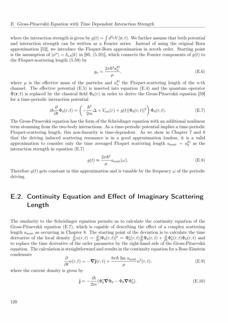
E. Gross-Pitaevskii Equation with Time Dependent Interaction Strength
where the interaction strength is given by g(t) =∫d3rV (r, t). We further assume that both potential
and interaction strength can be written as a Fourier series. Instead of using the original Bornapproximation [52], we introduce the Floquet-Born approximation in zeroth order. Starting pointis the assumption of |φn〉 = δn,0|k〉 in [80, (5.10)], which connects the Fourier components of g(t) tothe Floquet-scattering length (5.59) by
gn =2π~2aFl
n
µ, (E.6)
where µ is the effective mass of the particles and aFln the Floquet-scattering length of the n-th
channel. The effective potential (E.5) is inserted into equation (E.4) and the quantum operatorΨ(r, t) is replaced by the classical field Φ0(r) in order to derive the Gross-Pitaevskii equation [59]for a time-periodic interaction potential
i~∂
∂tΦ0(r, t) =
(− ~2
2m∆ + Vext(r) + g(t)|Φ0(r, t)|2
)Φ0(r, t). (E.7)
The Gross-Pitaevskii equation has the form of the Schrödinger equation with an additional nonlinearterm stemming from the two-body interactions. As a time-periodic potential implies a time-periodicFloquet-scattering length, this non-linearity is time-dependent. As we show in Chapter 7 and 8that the driving induced scattering resonance is in a good approximation lossless, it is a validapproximation to consider only the time averaged Floquet scattering length ascatt = aFl
0 as theinteraction strength in equation (E.7)
g(t) ≈ 2π~2
µascatt(ω). (E.8)
Therefore g(t) gets constant in this approximation and is tunable by the frequency ω of the periodicdriving.
E.2. Continuity Equation and Effect of Imaginary ScatteringLength
The similarity to the Schrödinger equation permits us to calculate the continuity equation of theGross-Pitaevskii equation (E.7), which is capable of describing the effect of a complex scatteringlength ascatt as occurring in Chapter 8. The starting point of the deviation is to calculate the timederivative of the local density ∂
∂tn(r, t) = ∂
∂t|Φ0(r, t)|2 = Φ∗0(r, t) ∂
∂tΦ0(r, t) + ∂
∂tΦ∗0(r, t)Φ0(r, t) and
to replace the time derivative of the order parameter by the right-hand side of the Gross-Pitaevskiiequation. The calculation is straightforward and results in the continuity equation for a Bose-Einsteincondensate
∂
∂tn(r, t) = −∇j(r, t) +
8π~ Im ascatt
µn2(r, t), (E.9)
where the current density is given by
j = − i~2m
(Φ∗0∇Φ0 − Φ0∇Φ∗0). (E.10)
120

E.2. Continuity Equation and Effect of Imaginary Scattering Length
0 10 20 30 40 50 60 70
time in A.U.
0
0.1
0.2
0.3
0.4
0.5
0.6
0.7
0.8
0.9
1
n in
A.U
n(t)
Figure E.1.: Plot of the homogeneous condensate density over the time with thevalues ~a
µ = −1 and n0 = 1.
Equation (E.9) states that the density of a Bose-Einstein condensate in a volume can be changed byeither a current flow through its surface or a decay due to an imaginary part of the scattering lengthascatt. The decay rate is proportional to the imaginary part of the scattering length and the squareof the density of the condensate. This can be made visible in the case of a homogeneous densityin equation (E.9). As the current vanishes in this case and the space dependency can be dropped,equation (E.9) simplifies to the ordinary differential equation
∂
∂tn(t) =
8π~ Im ascatt
µn2(t). (E.11)
The solution of this equation is derived straightforwardly by using the method of separation ofvariables to
n(t) =1
1n0− 8π~ Im ascatt
µ(t− t0)
. (E.12)
Here n0 describes the density at initial time t0. As due to the optical theorem the imaginary part ofthe scattering length is negative, (E.12) converges to zero for large times. A plot of equation (E.12)is seen in Figure E.1. Here the shape of the decay due to the imaginary part of the scattering lengthis visible.
121


Bibliography
[1] S. E. Pollack, D. Dries, R. G. Hulet, K. M. F. Magalhães, E. A. L. Henn, E. R. F. Ramos,M. A. Caracanhas, and V. S. Bagnato. Collective excitation of a Bose-Einstein condensate bymodulation of the atomic scattering length. Phys. Rev. A 81 053627 (2010).
[2] L. W. Clark, A. Gaj, L. Feng, and C. Chin. Collective emission of matter-wave jets fromdriven Bose-Einstein condensates. Nature Publishing Group 551 356–359 (2017).
[3] D. H. Smith. Inducing Resonant Interactions in Ultracold Atoms with a Modulated MagneticField. Phys. Rev. Lett 115 193002 (2015).
[4] A. G. Sykes, H. Landa, and D. S. Petrov. Two- and three-body problem with Floquet-drivenzero-range interactions. Phys. Rev. A 95 062705 (2017).
[5] D. Thuberg, S. A. Reyes, and S. Eggert. Quantum resonance catastrophe for conductancethrough a periodically driven barrier. Phys. Rev. B 93 180301 (2016).
[6] L. Dimou and F. H. M. Faisal. New class of resonance in the e + H+ scattering in an excimerlaser field. Phys. Rev. Lett. 59 872–875 (1987).
[7] H. Xian-Quan, X. Jie, L. Guang, and M. Yan. Introduction of the Coulomb dressed potentialinto atomic scattering. Chin. Chys. 16 3631 (2007).
[8] A. Emmanouilidou and L. E. Reichl. Floquet scattering and classical-quantum correspondencein strong time-periodic fields. Phys. Rev. A 65 033405 (2002).
[9] M. Terao-Dunseath and K. M. Dunseath. R -matrix Floquet theory for laser-assisted electron-atom scattering. J. Phys B 35 125 (2002).
[10] L. P. Rapoport and A. S. Kornev. Resonances and dichroism in the scattering of an electronin an intense laser field by the Coulomb potential. Journal of Experimental and TheoreticalPhysics 89 664–668 (1999).
[11] P. Kapitza. Dynamic stability of a pendulum when its point of suspension vibrates. Sov. Phys.JETP 21 588–592 ((1951)).
[12] P. Kapitza. Pendulum with a vibrating suspension. Usp. Fiz. Nauk 44 7–15 (1951).
123

Bibliography
[13] M. E. Semenov, D. V. Shevlyakova, and P. A. Meleshenko. Inverted pendulum under hystereticcontrol: Stability zones and periodic solutions. Nonlinear Dynamics 75 247–256 (2014).
[14] N. Ashcroft and N. Mermin. Solid state physics. Cengage Learning (2008).
[15] N. Goldman and J. Dalibard. Periodically driven quantum systems: Effective Hamiltoniansand engineered gauge fields. Phys. Rev. X 4 1–29 (2014).
[16] A. Eckardt, C. Weiss, and M. Holthaus. Superfluid-Insulator Transition in a PeriodicallyDriven Optical Lattice. Phys. Rev. Lett. 95 260404 (2005).
[17] A. Eckardt and M. Holthaus. AC-induced superfluidity. Europhys. Lett. 80 50004 (2007).
[18] A. Zenesini, H. Lignier, D. Ciampini, O. Morsch, and E. Arimondo. Coherent Control ofDressed Matter Waves. Phys. Rev. Lett. 102 100403 (2009).
[19] Dunlap, D. H. and Kenkre, V. M. Dynamic localization of a charged particle moving under theinfluence of an electric field. Phys. Rev. B 34 3625 (1986).
[20] B. J. Keay, S. Zeuner, S. J. Allen, K. D. Maranowski, A. C. Gossard, U. Bhattacharya, andM. J. W. Rodwell. Dynamic Localization, Absolute Negative Conductance, and Stimulated,Multiphoton Emission in Sequential Resonant Tunneling Semiconductor Superlattices. Phys.Rev. Lett. 75 4102–4105 (1995).
[21] G. Lenz, R. Parker, M. Wanke, and C. de Sterke. Dynamical localization and AC Blochoscillations in periodic optical waveguide arrays. Optics Communications 218 87 – 92 (2003).
[22] F. Dreisow, M. Heinrich, A. Szameit, S. Döering, S. Nolte, A. Tüennermann, S. Fahr, andF. Lederer. Spectral resolved dynamic localization in curved fs laser written waveguide arrays.Optics express 16 3474–3483 (2008).
[23] H. Lignier, C. Sias, D. Ciampini, Y. Singh, A. Zenesini, O. Morsch, and E. Arimondo. Dy-namical Control of Matter-Wave Tunneling in Periodic Potentials. Phys. Rev. Lett. 99 220403(2007).
[24] C. Sias, H. Lignier, Y. P. Singh, A. Zenesini, D. Ciampini, O. Morsch, and E. Arimondo.Observation of Photon-Assisted Tunneling in Optical Lattices. Phys. Rev. Lett. 100 040404(2008).
[25] A. Eckardt, M. Holthaus, H. Lignier, A. Zenesini, D. Ciampini, O. Morsch, and E. Arimondo.Exploring dynamic localization with a Bose-Einstein condensate. Phys. Rev. A 79 013611(2009).
[26] G. Jotzu, M. Messer, R. Desbuquois, M. Lebrat, T. Uehlinger, D. Greif, and T. Esslinger.
124
Bibliography
Experimental realization of the topological Haldane model with ultracold fermions. Nature 515237–240 (2014).
[27] N. Fläschner, D. Vogel, M. Tarnowski, B. S. Rem, D. S. Lühmann, M. Heyl, J. C. Budich,L. Mathey, K. Sengstock, and C. Weitenberg. Observation of dynamical vortices after quenchesin a system with topology. Nature Physics 14 1–4 (2017).
[28] B. Wang, F. N. Unal, and A. Eckardt. Floquet engineering of optical solenoids and quantizedcharge pumping along tailored paths in two-dimensional Chern insulators. arXiv:1802.06815(2018).
[29] J. Struck, C. Ölschläger, M. Weinberg, P. Hauke, J. Simonet, A. Eckardt, M. Lewenstein,K. Sengstock, and P. Windpassinger. Tunable Gauge Potential for Neutral and Spinless Par-ticles in Driven Optical Lattices. Phys. Rev. Lett. 108 225304 (2012).
[30] P. Hauke, O. Tieleman, A. Celi, C. Ölschläger, J. Simonet, J. Struck, M. Weinberg, P. Wind-passinger, K. Sengstock, M. Lewenstein, and A. Eckardt. Non-Abelian Gauge Fields andTopological Insulators in Shaken Optical Lattices. Phys. Rev. Lett. 109 145301 (2012).
[31] A. Eckardt. Colloquium: Atomic quantum gases in periodically driven optical lattices. Rev.Mod. Phys. 89 1–30 (2017).
[32] M. Grifoni and P. Hänggi. Driven quantum tunneling. Phys. Rep. 304 229–354 (1998).
[33] M. Holthaus. Floquet engineering with quasienergy bands of periodically driven optical lattices.J. Phys. B 49 013001 (2016).
[34] J. J. O´ Connor and E. F. Robertson. Gaston Floquet. In MacTutor History of Mathemat-ics archive. JOC/EFR, http://www-history.mcs.st-andrews.ac.uk/Biographies/Floquet.html(2005).
[35] G. Floquet. Sur les équations différentielles linéaires à coefficients périodiques. Annales scien-tifiques de l´École Normale Supérieure 12 47–88 (1883).
[36] H. Sambe. Steady states and quasienergies of a quantum-mechanical system in an oscillatingfield. Phys. Rev. A 7 2203–2213 (1973).
[37] I. Bloch, J. Dalibard, and W. Zwerger. Many-body physics with ultracold gases. Rev. Mod.Phys. 80 885–964 (2008).
[38] C. Chin, R. Grimm, P. Julienne, and E. Tiesinga. Feshbach resonances in ultracold gases. Rev.Mod. Phys. 82 1225–1286 (2010).
[39] I. Bloch. Ultracold quantum gases in optical lattices. Nature Physics 1 23–30 (2005).
125

Bibliography
[40] C. C. Bradley, C. A. Sackett, and R. G. Hulet. Bose-Einstein Condensation of Lithium:Observation of Limited Condensate Number. Phys. Rev. Lett. 78 985–989 (1997).
[41] S. L. Cornish, N. R. Claussen, J. L. Roberts, E. A. Cornell, and C. E. Wieman. Stable 85RbBose-Einstein Condensates with Widely Tunable Interactions. Phys. Rev. Lett. 85 1795–1798(2000).
[42] T. Bourdel, L. Khaykovich, J. Cubizolles, J. Zhang, F. Chevy, M. Teichmann, L. Tarruell,S. J. J. M. F. Kokkelmans, and C. Salomon. Experimental Study of the BEC-BCS CrossoverRegion in Lithium 6. Phys. Rev. Lett. 93 050401 (2004).
[43] M. Bartenstein, A. Altmeyer, S. Riedl, S. Jochim, C. Chin, J. H. Denschlag, and R. Grimm.Crossover from a Molecular Bose-Einstein Condensate to a Degenerate Fermi Gas. Phys. Rev.Lett. 92 120401 (2004).
[44] Q. Chen, J. Stajic, S. Tan, and K. Levin. BCS-BEC crossover: From high temperature super-conductors to ultracold superfluids. Phys. Rep 412 1 – 88 (2005).
[45] E. A. Donley, N. R. Claussen, S. T. Thompson, and C. E. Wieman. Atom-molecule coherencein a Bose-Einstein condensate. Nature 417 529–533 (2002).
[46] S. T. Thompson, E. Hodby, and C. E. Wieman. Ultracold Molecule Production via a ResonantOscillating Magnetic Field. Phys. Rev. Lett. 95 190404 (2005).
[47] W. Cairncross and A. Pelster. Parametric resonance in Bose-Einstein condensates with periodicmodulation of attractive interaction. Europhys. J. D 68 106 (2014).
[48] I. Vidanović, A. Balaž, H. Al-Jibbouri, and A. Pelster. Nonlinear Bose-Einstein-condensatedynamics induced by a harmonic modulation of the s-wave scattering length. Phys. Rev. A 84013618 (2011).
[49] S. A. Reyes, D. Thuberg, D. Pérez, C. Dauer, and S. Eggert. Transport through an AC-drivenimpurity: Fano interference and bound states in the continuum. New J. Phys. 19 043029(2017).
[50] U. Fano. Effects of Configuration Interaction on Intensities and Phase Shifts. Phys. Rev. 1241866–1878 (1961).
[51] A. E. Miroshnichenko and Y. S. Kivshar. Engineering Fano resonances in discrete arrays.Phys. Rev. E 72 056611 (2005).
[52] C. Pethick and H. Smith. Bose-Einstein Condensation in Dilute Gases. Cambridge UniversityPress (2002).
126
Bibliography
[53] C. Timm. Quantentheorie 2. TU Dresden, Institut für Theoretische Physik (2015). Abgerufenam 29.09.2017, 12:18.
[54] H. Korsch. Mathematische Ergänzungen zur Einführung in die Physik. Binomi (2004).
[55] A. Pelster. Bose-Einstein-Kondensation. Universität Duisburg-Essen, http://users.physik.fu-berlin.de/ pelster/Vorlesungen/WS1213/bec.pdf (2004).
[56] H. Friedrich. Scattering Theory. Springer Berlin Heidelberg (2015).
[57] N. Mott and H. Massey. The Theory of Atomic Collisions, by N.F. Mott and H.S.W. Massey.3rd Edition. Clarendon Press (1965).
[58] R. Newton. Scattering theory of waves and particles. International series in pure and appliedphysics. McGraw-Hill (1966).
[59] L. Pitaevskii and S. Stringari. Bose-Einstein Condensation. International Series of Monographson Physics. Clarendon Press (2003).
[60] B. Bransden and C. Joachain. Physics of Atoms and Molecules. Pearson Education. PrenticeHall (2003).
[61] H. Feshbach. Unified theory of nuclear reactions. Ann. Phys. (New York) 5 357 390 (1958).
[62] H. Feshbach. A unified theory of nuclear reactions. II. Ann. Phys. (New York) 19 287–313(1962).
[63] A. J. Moerdijk, B. J. Verhaar, and A. Axelsson. Resonances in ultracold collisions of 6Li, 7Li,and 23Na. Phys. Rev. A 51 4852–4861 (1995).
[64] E. Timmermans, P. Tommasini, M. Hussein, and A. Kerman. Feshbach resonances in atomicBose-Einstein condensates. Phys. Rep. 315 199 – 230 (1999).
[65] S. Inouye, M. R. Andrews, J. Stenger, H.-J. Miesner, D. M. Stamper-Kurn, and W. Ketterle.Observation of Feshbach resonances in a Bose-Einstein condensate. Nature 392 151 (1998).
[66] P. Courteille, R. S. Freeland, D. J. Heinzen, F. A. van Abeelen, and B. J. Verhaar. Observationof a Feshbach Resonance in Cold Atom Scattering. Phys. Rev. Lett. 81 69–72 (1998).
[67] P. O. Fedichev, Y. Kagan, G. V. Shlyapnikov, and J. T. M. Walraven. Influence of NearlyResonant Light on the Scattering Length in Low-Temperature Atomic Gases. Phys. Rev. Lett.77 2913–2916 (1996).
127

Bibliography
[68] F. K. Fatemi, K. M. Jones, and P. D. Lett. Observation of Optically Induced Feshbach Reso-nances in Collisions of Cold Atoms. Phys. Rev. Lett. 85 4462–4465 (2000).
[69] O. Thomas, C. Lippe, T. Eichert, and H. Ott. Experimental realization of a Rydberg opticalFeshbach resonance in a quantum many-body system. arXiv:1712.05263 (2017).
[70] M. Theis, G. Thalhammer, K. Winkler, M. Hellwig, G. Ruff, R. Grimm, and J. H. Denschlag.Tuning the Scattering Length with an Optically Induced Feshbach Resonance. Phys. Rev. Lett.93 123001 (2004).
[71] A. J. Moerdijk, B. J. Verhaar, and T. M. Nagtegaal. Collisions of dressed ground-state atoms.Phys. Rev. A 53 4343 (1996).
[72] A. M. Kaufman, R. P. Anderson, T. M. Hanna, E. Tiesinga, P. S. Julienne, and D. S. Hall.Radio-frequency dressing of multiple Feshbach resonances. Phys. Rev. A 80 050701 (2009).
[73] S. V. Alyabyshev, T. V. Tscherbul, and R. V. Krems. Microwave-laser-field modification ofmolecular collisions at low temperatures. Phys. Rev. A 79 060703 (2009).
[74] T. M. Hanna, E. Tiesinga, and P. S. Julienne. Creation and manipulation of Feshbach reso-nances with radio-frequency radiation. New J. Phys. 12 (2010).
[75] T. V. Tscherbul, T. Calarco, I. Lesanovsky, R. V. Krems, A. Dalgarno, and J. Schmiedmayer.RF-field-induced Feshbach resonances. Phys. Rev. A 81 1–4 (2010).
[76] T. Xie, G.-R. Wang, Y. Huang, W. Zhang, and S.-L. Cong. The radio frequency field modulationof magnetically induced heteronuclear Feshbach resonance. J. Phys. B 45 145302 (2012).
[77] D. J. Papoular, G. V. Shlyapnikov, and J. Dalibard. Microwave-induced Fano-Feshbach reso-nances. Phys. Rev. A 81 041603 (2010).
[78] D. J. Owens, T. Xie, and J. M. Hutson. Creating Feshbach resonances for ultracold moleculeformation with radio-frequency fields. Phys. Rev. A 94 023619 (2016).
[79] Y. Ding, J. P. D’Incao, and C. H. Greene. Effective control of cold collisions with radio-frequency fields. Phys. Rev. A 95 022709 (2017).
[80] D. H. Smith. Resonant Floquet scattering of ultracold atoms. Ph.D. thesis, The Ohio StateUniversity (2016).
[81] A. Mohapatra and E. Braaten. Harmonic and subharmonic association of universal dimers ina thermal gas. Phys. Rev. A 92 013425 (2015).
[82] T. Dittrich. Quantum transport and dissipation. Wiley-VCH (1998).
128

Bibliography
[83] H. Ibach, Harald; Lüth. Festkörperphysik. Springer Verlag Heidelberg, 7 edition (2009).
[84] R. Shankar. Principles of Quantum Mechanics. Springer US, 2. edition edition (2008).
[85] M. Abramowitz and I. A. Stegun, editors. Handbook of Mathematical Functions with Formulas,Graphs, and Mathematical Tables. New York: Dover, 9th printing edition (1972).
[86] J. R. Taylor. Scatterning Theory: The Quantum Theory on Nonrelativistic Collisions. JohnWiley & Sons, Inc. (1972).
[87] A. Russomanno and G. E. Santoro. Floquet resonances close to the adiabatic limit and theeffect of dissipation. J Stat. Mech. 2017 103104 (2017).
[88] H. Haken. Laser Theory. Springer Berlin Heidelberg (1970).
[89] MATLAB Documentary: Backslash Operator. https://de.mathworks.com/help/matlab/ref/mldivide.html.
[90] D. Thuberg. AC-Driven Impurities in Nanoscale Systems. Ph.D. thesis, Pontifical CatholicUniversity of Chile, Institute of Physics (2017).
[91] C. W. Hsu, B. Zhen, A. D. Stone, J. D. Joannopoulos, and M. Soljačić. Bound states in thecontinuum. Nature Rev. Mat. 1 16048 (2016).
[92] J. von Neumann and E. Wigner. Über Merkwurdige Diskrete Eigenwerte. Phys. Z. 30 465–467(1929).
[93] F. H. Stillinger and D. R. Herrick. Bound states in the continuum. Phys. Rev. A 11 446–454(1975).
[94] H. Friedrich and D. Wintgen. Physical realization of bound states in the continuum. Phys.Rev. A 31 3964–3966 (1985).
[95] H. Friedrich and D. Wintgen. Interfering resonances and bound states in the continuum. Phys.Rev. A 32 3231–3242 (1985).
[96] C. González-Santander, P. A. Orellana, and F. Domínguez-Adame. Bound states in the con-tinuum driven by AC fields. Europhys. Lett. 102 17012 (2013).
[97] S. Longhi and G. D. Valle. Floquet bound states in the continuum. Scient. Rep. 3 (2013).
[98] P. F. Bagwell and R. K. Lake. Resonances in transmission through an oscillating barrier. Phys.Rev. B 46 15329–15336 (1992).
129

Bibliography
[99] D. F. Martinez and L. E. Reichl. Transmission properties of the oscillating δ-function potential.Phys. Rev. B 64 245315 (2001).
[100] MATLAB Documentary: Evaluating Goodness of Fit. https://de.mathworks.com/help/curvefit/evaluating-goodness-of-fit.html.
[101] E. W. Weisstein. "Square Root." From MathWorld–A Wolfram Web Resource.
[102] N. R. Claussen, S. J. J. M. F. Kokkelmans, S. T. Thompson, E. A. Donley, E. Hodby, andC. E. Wieman. Very-high-precision bound-state spectroscopy near a 85Rb Feshbach resonance.Phys. Rev. A 67 060701 (2003).
[103] S. Longhi. Non-Hermitian Floquet invisibility. Europhys. Lett. 117 10005 (2017).
[104] D. M. Stamper-Kurn, M. R. Andrews, A. P. Chikkatur, S. Inouye, H.-J. Miesner, J. Stenger,and W. Ketterle. Optical Confinement of a Bose-Einstein Condensate. Phys. Rev. Lett. 802027–2030 (1998).
[105] Y. Kawaguchi and M. Ueda. Spinor Bose-Einstein condensates. Phys. Rep. 520 253 – 381(2012). Spinor Bose–Einstein condensates.
[106] L. . E. Sadler, J. M. Higbie, S. R. Leslie, M. Vengalattore, and D. M. Stamper-Kurn. Sponta-neous symmetry breaking in a quenched ferromagnetic spinor Bose-Einstein condensate. Nature5 443 312–315 (2006).
[107] F. Schmidt, D. Mayer, Q. Bouton, D. Adam, T. Lausch, N. Spethmann, and A. Widera.Quantum spin dynamics of individual neutral impurities coupled to a Bose-Einstein condensate.arXiv:1802.08702v1 (2018).
[108] F. Schmidt. Private Communications. TU Kaiserslautern, AG Widera (2018).
[109] P. Soltan-Panahi. Thermodynamic Properties of F=1 Spinor Bose-Einstein Condensates.Diplomarbeit, Freien Universität Berlin (2006).
[110] C. Jörg, F. Letscher, M. Fleischhauer, and G. von Freymann. Dynamic defects in photonicFloquet topological insulators. New J. Phys. 19 083003 (2017).
[111] C. Jörg. Erste Schritte in Richtung optischer topologischer Isolatoren durch direktes Laser-schreiben. Diplomarbeit, Technische Universität Kaiserslautern (2015).
[112] F. Bleckmann, Z. Cherpakova, S. Linden, and A. Alberti. Spectral imaging of topological edgestates in plasmonic waveguide arrays. Phys. Rev. B 96 045417 (2017).
130

Bibliography
[113] M. C. Rechtsman, J. M. Zeuner, Y. Plotnik, Y. Lumer, D. Podolsky, F. Dreisow, S. Nolte,M. Segev, and A. Szameit. Photonic Floquet topological insulators. Nature 496 196–200 (2013).
[114] F. Letscher. Topologische Zustände in Bosonischen Gittermodellen. Diplomarbeit, TechnischeUniversität Kaiserslautern (2014).
[115] C. Jörg and F. Letscher. Privat Communications. Technische Universität Kaiserslautern, AGvon Freymann and AG Fleischhauer (2018).
[116] J. K. Asbóth, L. Oroszlány, and A. Pályi. A Short Course on Topological Insulators. SpringerInternational Publishing (2016).
[117] Z. Cherpakova, C. Jörg, C. Dauer, F. Letscher, M. Fleischhauer, S. Eggert, S. Linden, andG. von Freymann. Private Communications (2018).
[118] G. Breit. The Scattering of Slow Neutrons by Bound Protons. I. Methods of Calculation. Phys.Rev. 71 215–231 (1947).
[119] K. Huang and C. N. Yang. Quantum-Mechanical Many-Body Problem with Hard-Sphere In-teraction. Phys. Rev. 105 767–775 (1957).
[120] A. Zangwill. Modern Electrodynamics. Modern Electrodynamics. Cambridge University Press(2013).
[121] K. R. Waters, J. Mobley, and J. G. Miller. Causality-imposed (Kramers-Kronig) relationshipsbetween attenuation and dispersion. IEEE Transactions on Ultrasonics, Ferroelectrics, andFrequency Control 52 822–833 (2005).
[122] V. Lucarini, J. Saarinen, K. Peiponen, and E. Vartiainen. Kramers-Kronig Relations in OpticalMaterials Research. Springer Series in Optical Sciences. Springer Berlin Heidelberg (2006).
[123] A. Messiah. Quantenmechanik. Walter de Gruyter, 1. edition (1976).
131

Acknowledgement
At this point I want to say thanks to people, who supported me during my studies. At first I wantto show my gratitude to Prof. Dr. Sebastian Eggert for the deep discussions and the supervision,which helped me to find a good path. I also want to thank Priv. Doz. Dr. habil. Axel Pelster forhis great support, his fast answer to questions, the large amount of helpful discussions and his hugeenthusiasm, which encouraged me during the time of the thesis. I also thank Dr. Imke Scheiderfor her helpful opinion in discussions. I thank all members of the group Eggert for the inspiringdiscussions and fast and helpful answer of questions that occurred. I want to thank HamidrezaKazemi, Martin Bonkhoff, Polina Matveeva, Dr. Shaon Sahoo, Dr. Milan Radonjic, Dr. Shijie Hu,Enrico Stein and Kevin Jägering for being friendly colleagues.
I show my gratitude to Christina Jörg, Fabian Letscher and Zlata Cherpakova for for the initia-tion and valuable collaboration in a joint research project. I also want to thank Felix Schmidt,Daniel Adam and Prof. Dr. Artur Widera for the interest in my investigations, which showed up intrend-setting discussions during the time of my thesis. I also want to thank Daniel Thuberg for thevaluable discussions during his visit.
I show deepest appreciation to Enrico, who I know since the beginning of my studies. We haddetailed physical discussions during our studies and he helped me with many problems. I want tothank all my friends for the great time we had and the nice events we visited.
I say thanks to my parents Jutta and Günter for the never-ending support and the always openear for my problems. I can only extend this to the whole family and thank all of them for theirheartening in the last years. At last I want thank Katharina for always being on my side also inhard times.