Tuning GaussSieve for Speed

Robert Fitzpatrick1, Christian Bischof2, Johannes Buchmann3, OzgurDagdelen3, Florian Gopfert3, Artur Mariano2 and Bo-Yin Yang1

1 Institute of Information Science, Academia Sinica, Taipei, Taiwan2 Institute for Scientific Computing TU Darmstadt, Darmstadt, Germany

3 CASED, TU Darmstadt, Darmstadt, Germany

Abstract. The area of lattice-based cryptography is growing ever-moreprominent as a paradigm for quantum-resistant cryptography. One ofthe most important hard problem underpinning the security of lattice-based cryptosystems is the shortest vector problem (SVP). At present,two approaches dominate methods for solving instances of this problemin practice: enumeration and sieving. In 2010, Micciancio and Voulgarispresented a heuristic member of the sieving family, known as GaussSieve,demonstrating it to be comparable to enumeration methods in practice.With contemporary lattice-based cryptographic proposals relying largelyon the hardness of solving the shortest and closest vector problems inideal lattices, examining possible improvements to sieving algorithmsbecomes highly pertinent since, at present, only sieving algorithms havebeen successfully adapted to solve such instances more efficiently than inthe random lattice case. In this paper, we propose a number of heuristicimprovements to GaussSieve, which can also be applied to other sievingalgorithms for SVP.

1 Introduction

Lattice-based cryptography is gaining increasing traction and popularity as abasis for post-quantum cryptography, with the Shortest Vector Problem (SVP)being one of the most important computational problems on lattices. Its difficultyis closely related to the security of most lattice-based cryptographic constructionsto date. The SVP consists in finding a shortest (with respect to a particular,usually Euclidean, norm) non-zero lattice point in a given lattice.

For solving SVP instances, we have a choice of algorithms available. In re-cent works, heuristic variants of Kannan’s simple enumeration algorithm havedominated. The original algorithm [11] solves SVP (deterministically) with timecomplexity n

n2 +o(n) (n being the lattice dimension). More recent works (such

as [7]) allow probabilistic SVP solution, sacrificing guaranteed solution for run-time improvements.

A more recently-studied family of algorithms is known as lattice sieving al-gorithms, introduced in the 2001 work of Ajtai et al. [4]. In 2008, Nguyen andVidick [20] presented a careful analysis of the algorithm of Ajtai et al., show-ing it to possess time complexity of 25.90n+o(n) and space complexity 22.95n+o(n).

Heuristic variants of [20], which run significantly faster than proven lower boundsare presented in [20,26,27]. In 2010, Micciancio and Voulgaris [18] proposed twonew algorithms: ListSieve and a heuristic derivation known as GaussSieve, withGaussSieve being the most practical sieving algorithm known at present. Whileno runtime bound is known for GaussSieve, the use of a simple heuristic stoppingcondition, in practice, appears effective with no cases being known (to the bestof our knowledge) in which GaussSieve fails to return a shortest non-zero vector.

For purposes of enhanced communication, computation and memory com-plexity, many recent lattice-based cryptographic proposals employ ideal latticesrather than “random” lattices. Ideal lattices, in brief, possess significant ad-ditional structure which allows much more attractive implementation of saidproposals. However, as with any introduction of structure, the question of anysimultaneously-introduced weakening of the underlying problems arises. In 2011,Schneider [21] illustrated that (following a suggestion in the work of Micciancioand Voulgaris [18]) one can take advantage of the additional structure present inideal lattices in a simple way to obtain substantial speedups for such cases. In-terestingly, no such comparable techniques are known for other SVP algorithms,with only sieving algorithms appearing to be capable of exploiting the additionalstructure exposed in ideal lattices.

Another attractive feature of sieving algorithms is their relative amenabilityto parallelization. Also in 2011, Milde and Schneider [19] proposed a parallelimplementation of GaussSieve, though the methodology used limited the numberof threads to about ten, before no substantial further speedups could be obtained.In 2013, Ishiguro et al. [10] proposed a somewhat more natural parallelization ofGaussSieve, allowing a much larger number of threads. Using such an approach,they report the solution of the 128-dimensional ideal lattice challenge [2] in30,000 CPU hours. Currently, the most efficient GaussSieve implementation (ofwhich details have been published) is due to Mariano et al [16] who implementedGaussSieve with a particular effort to avoid resource contention. In this work,we exhibit several further speedups which can be obtained both in the randomand ideal lattice cases.

While the security of most lattice-based cryptographic constructions relieson the difficulty of approximate versions of the related Closest Vector Problem(CVP) and SVP, the importance of improving exact SVP solvers stems fromtheir use (following Schnorr’s hierarchy [22]) in the construction of approximateCVP/SVP solvers. Thus, any improvements, both theoretically and experimen-tally, in exact SVP solvers can lead to a need for re-appraisal of proposed pa-rameterizations.

Our Contribution. In this work, we highlight several practical improvementsthat are applicable to other sieving algorithms. In particular, we propose thefollowing optimizations, which we incorporated into GaussSieve:

– We correct an error in the Gaussian sampler of the reference implementa-tion of Voulgaris and propose an optimized Gaussian sampler in which wedynamically adapt the Gaussian parameter used during the execution of the

2

algorithm. Our experiments show that GaussSieve with our optimized Gaus-sian sampler requires significantly fewer iterations to terminate and leads toa speedup of up to 3.0× over the corrected reference implementation in ran-dom lattices in dimension 60-70.

– The use of multiple randomized bases to seed the list before running the siev-ing process offers substantial efficiency gains. Indeed, the speedup appearsto grow linearly in the dimension of the underlying lattice.

– We introduce a very efficient heuristic to compute a first approximation to theangle between two vectors in order to test cheaply whether there is the needto compute full inner products for the reduction process. This optimizationis possibly of independent interest beyond sieving algorithms.

We note that our improvements can be integrated into parallel versions ofGaussSieve without complication or restriction.

2 Background and Notation

A (full-rank) lattice Λ in Rn is a discrete additive subgroup. For a general intro-duction, the reader is referred to [17]. We view a lattice as being generated bya (non-unique) basis B = {b0, . . . ,bn−1} ⊂ Rn of linearly-independent vectors.We assume that the vectors b0, . . . ,bn−1 form the rows of the n× n matrix B.That is,

Λ = L(B) = Zn ·B =

{n−1∑i=0

xi · bi | x0, . . . , xn−1 ∈ Z

}.

The rank of a lattice Λ is the dimension of the linear span span(Λ) of Λ. Thebasis B is not unique, and thus we call two bases B and B′ equivalent if andonly if B′ = BU where U is a unimodular matrix, i.e., an integer matrix with|det(U)| = 1. We note that such unimodular matrices form the general lineargroup GLn(Z). Being a discrete subgroup, in any lattice there exists a subset ofvectors which possess minimal (non-zero) norm amongst all vectors. When askedto solve the shortest vector problem, we are given a lattice basis and asked todeliver a member of this subset. SVP is known to be NP-hard under randomizedreductions [3].

Random Lattices. Throughout this work, we rely on experiments with “random”lattices. However, the question of what a “random” lattice is and how to generatea random basis of one are non-trivial. In a mathematical sense, an answer to thedefinition of a random lattice follows from a work in 1945 by Siegel [24], withefficient methods for sampling such random lattices being proposed, for instance,by Goldstein and Mayer [9]. In this work, all experiments were conducted withGoldstein-Mayer lattices, as provided by the TU Darmstadt Lattice Challengeproject. For more details, the reader is directed to [8].

Definition 1. Given two vectors v,w in a lattice Λ, we say that v,w are Gauss-reduced if

min(‖v ±w‖) ≥ max(‖v‖, ‖w‖) .

3

Lattice Basis Reduction. A given lattice has an infinite number of bases. Theaim of lattice basis reduction is to transform a given lattice basis into one whichcontains vectors which are both relatively short and relatively orthogonal. Suchbases, in some sense, allow easier and/or more accurate solutions of approxima-tion variants of SVP or its related problem, the Closest Vector Problem (CVP).In practice, the most effective arbitrary-dimension lattice basis reduction al-gorithms are descendants of the LLL algorithm [14], with the Block-Korkine-Zolotarev (BKZ) family [22,5] (or framework) of algorithms being the most ef-fective in practice. The LLL and BKZ algorithms rely on successive exact SVPsolution in a number of projected lattices. These projected lattices are two-dimensional in the case of LLL and of arbitrary dimension in the case of BKZ –the (maximal) projected lattice dimension being termed the “blocksize” in BKZ.For more details, the reader is referred to [6].

Balls and Spheres. We define the Euclidean n-sphere Sn(x, r) centered at x ∈Rn+1 and of radius r by Sn(x, r) := {y ∈ Rn+1 : ‖ x − y ‖= r}. The (open)Euclidean n-ball Bn(x, r) centered at x ∈ Rn and of radius r is defined to beBn(x, r) := {y ∈ Rn : ‖ x− y ‖< r}.

Gaussians. The discrete Gaussian distribution with parameter s over a latticeΛ is defined to be the probability distribution with support Λ which, for eachx ∈ Λ, assigns probability proportional to exp(−π‖x‖2/s2).

Miscellany. We use ⊕ to denote the bitwise XOR operation and use a∠b todenote the angle between vectors a and b. Given a binary vector a, we use w(a)to denote the Hamming weight of a.

3 The GaussSieve Algorithm

In 2010, Micciancio and Voulgaris [18] introduced the GaussSieve algorithm.GaussSieve is a heuristic efficient variant of the ListSieve algorithm. In contrastto GaussSieve, for ListSieve there exist provable bounds on the running timeand space requirements. Algorithm 1 depicts the GaussSieve algorithm in moredetail.

GaussSieve operates upon a supplied lattice basis B. It utilizes a dynamic listL of lattice points. At each iteration, GaussSieve samples a new lattice point –typically with Klein’s algorithm [12] – and attempts to reduce that vector againstvectors in the list L. By “reducing” we mean adding an integer multiple of a listvector such that the norm of the resulting vector is reduced. Once the vectorcannot be reduced further by list members, the resulting vector is incorporatedin the list. Afterwards, all the vectors in the list L are tested to determine if theycan be reduced against this new vector. If so, those vectors are removed to a stackS, with the stack playing the role of Klein’s algorithm in subsequent iterationstill it is depleted. This ensures that all vectors in the list L remain pairwiseGauss-reduced at any point during the execution of the algorithm. Eventually,

4

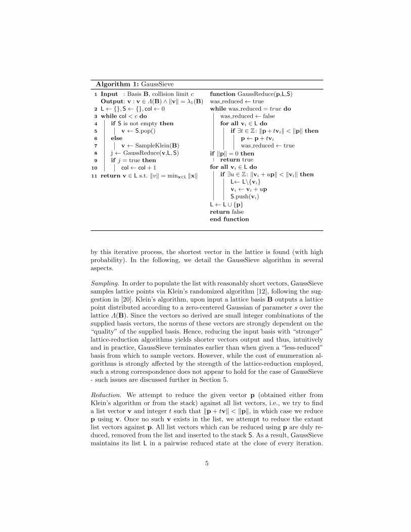
Algorithm 1: GaussSieve

1 Input : Basis B, collision limit cOutput: v : v ∈ Λ(B) ∧ ‖v‖ = λ1(B)

2 L← {}, S← {}, col← 03 while col < c do4 if S is not empty then5 v ← S.pop()6 else7 v ← SampleKlein(B)8 j ← GaussReduce(v,L,S)9 if j = true then

10 col← col + 1

11 return v ∈ L s.t. ‖v‖ = minx∈L ‖x‖

function GaussReduce(p,L,S)was reduced← truewhile was reduced = true do

was reduced← falsefor all vi ∈ L do

if ∃t ∈ Z : ‖p+ tvi‖ < ‖p‖ thenp← p + tvi

was reduced← true

if ‖p‖ = 0 thenreturn true

for all vi ∈ L doif ∃u ∈ Z : ‖vi + up‖ < ‖vi‖ then

L← L\{vi}vi ← vi + upS.push(vi)

L← L ∪ {p}return falseend function

by this iterative process, the shortest vector in the lattice is found (with highprobability). In the following, we detail the GaussSieve algorithm in severalaspects.

Sampling. In order to populate the list with reasonably short vectors, GaussSievesamples lattice points via Klein’s randomized algorithm [12], following the sug-gestion in [20]. Klein’s algorithm, upon input a lattice basis B outputs a latticepoint distributed according to a zero-centered Gaussian of parameter s over thelattice Λ(B). Since the vectors so derived are small integer combinations of thesupplied basis vectors, the norms of these vectors are strongly dependent on the“quality” of the supplied basis. Hence, reducing the input basis with “stronger”lattice-reduction algorithms yields shorter vectors output and thus, intuitivelyand in practice, GaussSieve terminates earlier than when given a “less-reduced”basis from which to sample vectors. However, while the cost of enumeration al-gorithms is strongly affected by the strength of the lattice-reduction employed,such a strong correspondence does not appear to hold for the case of GaussSieve- such issues are discussed further in Section 5.

Reduction. We attempt to reduce the given vector p (obtained either fromKlein’s algorithm or from the stack) against all list vectors, i.e., we try to finda list vector v and integer t such that ‖p + tv‖ < ‖p‖, in which case we reducep using v. Once no such v exists in the list, we attempt to reduce the extantlist vectors against p. All list vectors which can be reduced using p are duly re-duced, removed from the list and inserted to the stack S. As a result, GaussSievemaintains its list L in a pairwise reduced state at the close of every iteration.

5

In the following iteration, if the stack contains at least one element, we pop avector from the stack in lieu of employing Klein’s algorithm.

Stopping criteria. Given that one cannot prove (at present) that GaussSieveterminates, stopping conditions for GaussSieve must be chosen in a heuristicway, chosen such that any further reduction in the norm of the shortest vectorfound is unlikely to occur. In [18], it is suggested to terminate the algorithmafter a certain number of successively-sampled vectors are all reduced to zerousing the extant list, with 500 such consecutive zero reductions being mentionedas a possible choice in practice. In Voulgaris’ implementation, a stopping con-dition is employed which depends on the maximal list size encountered. In ourexperiments we follow the suggestions of [18] in this regard.

Complexity. As with all sieving algorithms, the complexity of GaussSieve islargely determined by arguments related to sphere packing and the KissingNumber - the maximum number of equivalent hyperspheres in n dimensionswhich are permitted to touch another equivalent hypersphere yet not intersect.With practical variants of GaussSieve, as dealt with here, no complexity boundis known due to the possibility of perpetual reductions of vectors to zero withouta shortest vector being found. For further details, we direct the reader to [18].

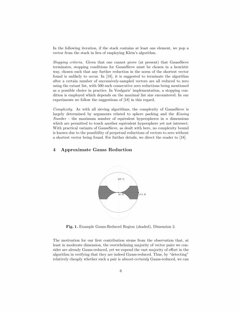
4 Approximate Gauss Reduction

(0, 1)

(0, 0) (1.5, 0)

Fig. 1. Example Gauss-Reduced Region (shaded), Dimension 2.

The motivation for our first contribution stems from the observation that, atleast in moderate dimension, the overwhelming majority of vector pairs we con-sider are already Gauss-reduced, yet we expend the vast majority of effort in thealgorithm in verifying that they are indeed Gauss-reduced. Thus, by “detecting”relatively cheaply whether such a pair is almost-certainly Gauss-reduced, we can

6

obtain substantial (polynomial) speedups at the cost of possibly erring (almostinconsequentially) with respect to a few pairs.

We now make an idealizing assumption, namely the random ball assump-tion (as appears in [25]) that we can gain insights into the behavior of latticealgorithms by assuming that lattice vectors are sampled uniformly at randomfrom the surface of an Euclidean ball of a given radius. As in [25], we term thisthe “random ball model”. For intuition, Figure 1 shows the region (shaded) ofvectors in the ball B2(0, 1.5) which are Gauss-reduced with respect to the vector(0, 1).

Lemma 1. Given a vector v ∈ Rn of (Euclidean) norm r sampled from atrandom from Sn−1(0, r) and a second vector w sampled independently at randomfrom Sn−1(0, r′) (where r′ is a second radius), the probability that w is Gauss-reduced with respect to v is

1− I1−(r/2r′)2(n− 1

2,

1

2

)where hh := r′−r/2 and Ix(a, b) denotes the regularized incomplete beta function.

Proof. We assume, without loss of generality, that r′ ≥ r, otherwise, we swap vand w. The surface area of the n-sphere of radius r′ (denoted Sn−1(0, r′)) is

Sn−1(0, r′) =nπn/2r′n−1

Γ (1 + n2 )

.

Then, the points from this sphere which are Gauss-reduced with respect to v aredetermined by the relative complement of Sn−1(0, r′) with the hyper-cylinder ofradius

√r′2 − r2/4 , of which both the origin and v lie on the center-line. We can

calculate the surface area of this relative complement by subtracting the surfacearea of a certain hyperspherical cap from the surface area of a hemisphere ofthe hypersphere of radius r′. Specifically, let us consider only one hemisphereof Sn−1(0, r′). Considering the hyperspherical cap of height hh := r′ − r/2, thiscap has surface area

1

2Sn−1(0, r′)I1−(r/2r′)2

(n− 1

2,

1

2

),

where Ix(a, b) denotes the regularized incomplete beta function:

Ix(a, b) :=

∞∑i=a

(a+ b− 1

i

)xi(1− x)a+b−1−i .

Thus, the relative complement has surface area

1

2Sn−1(0, r′)

(1− I1−(r/2r′)2

(n− 1

2,

1

2

))

7

and hence, the probability of obtaining a Gauss-reduced vector is

1− I1−(r/2r′)2(n− 1

2,

1

2

)) .

ut

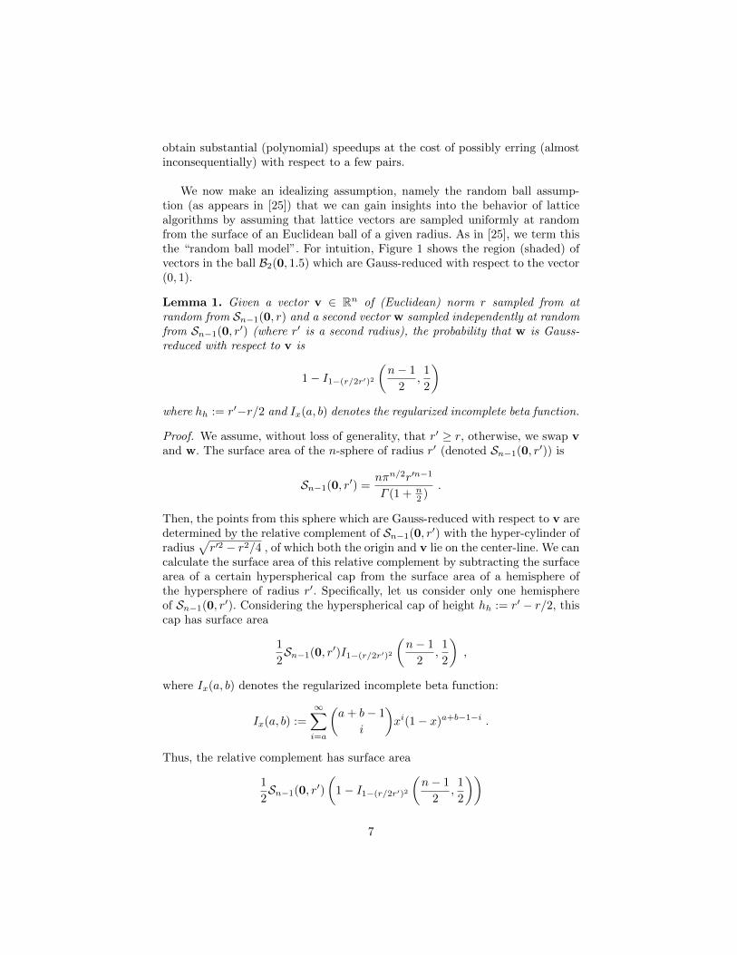
For instance, Figure 2 gives the probability of two vectors being a priori Gauss-reduced with increasing dimension in the case of r = 1000 and r′ = 1100. Bya priori Gauss-reduced, we mean that two vectors, sampled at random fromzero-centered spheres of respective radii, are Gauss-reduced with respect to eachother. These illustrative values are chosen to be representative of the similar-norm pairs of vectors which comprise the vast majority of attempted reductionsin GaussSieve.

20 40 60 800

0.5

1

dimension(n)

pro

babilit

yb

eing

Gauss

-red

uce

d

Fig. 2. Example probabilities of a priori Gauss-reduction, r = 1000, r′ = 1100.

If we are given two such vectors, we can easily determine whether they areGauss-reduced by considering the angle θ between them. It follows simply fromelementary Euclidean geometry that if the following condition is satisfied, theyare Gauss-reduced:

|π2− θ| ≤ arcsin(r/2r′)

Thus, if we can “cheaply” determine an approximate angle, we can tell with goodconfidence whether they are indeed Gauss-reduced or not. We note that, whilewe do not believe one can prove similar arguments to the above in the context oflattices, the behavior appears indistinguishable for random lattices in practice.Indeed, we also experimented with vector pairs sampled from random latticebases using Klein’s algorithm and obtained identical behavior to that illustratedin Figures 2 and 3. For determining such approximate angles, we investigated twoapproaches: a) computing the angle between restrictions of vectors to subspacesand b) exploiting correlations between the XOR + population count of the signbits of a pair of vectors and the angle between them. We only report the latterapproach, which appears to offer superior results in practice.

8

Using XOR and Population Count as a First Approximation to theAngle. Given a vector a ∈ Zn we define a ∈ Zn

2 such that ai = sgn(ai). Here,we define

sgn(a) : R→ {0, 1} by sgn(a) =

{0 if a < 0

1 otherwise

and define the normalized XOR followed by population count of a and b to be

sip(a,b) : Rn × Rn → R+ by sip(a,b) = w(a⊕ b)/n

Based on Assumption 1, we can use the XOR + population count of a and b as afirst approximation to the angle between a and b when their norms are relativelysimilar. The attraction of using sip(a,b) as a first approximation to a∠b is theneed to only compute an XOR of two binary vectors followed by a populationcount, operations which can be implemented efficiently. For intuition, considerthe first components a1, b1 of vectors a and b, respectively. If sgn(a1)⊕sgn(b1) =1 then the signs of these components are different and are the same otherwise.Clearly, in higher dimensions, when sampling uniformly at random from a zero-centered sphere, the expected number of such individual XORs would be n/2,hence E[sip(a,b)] = 1/2. If sip(a,b) = 1, then all components of both vectors liein the same intersection of the sphere with a given orthant and thus we mightexpect that the angle between these two vectors has a good chance of beingrelatively small. The analogous case of sip(a,b) = 0 corresponds to taking thenegative of one of the vectors. Conversely, since the expected value of sip(a,b) is1/2, we expect this to coincide with the heuristic that, in higher dimensions, mostvectors sampled uniformly at random from a zero-centered sphere are almostorthogonal. Again, we stress that these arguments are given purely for intuitionand appear to work well in practice, as posited in Assumption 1:

Assumption 1 [Informal] Let n� 2. Then, given a random (full-rank) latticeΛ of dimension n and two vectors a,b ∈ Λ of “similar” norms sampled uni-formly at random from the set of all such lattice vectors, the distribution of thenormalized sign XOR + population count of these vectors sip(a,b) and the anglebetween them can be approximated by a bivariate Gaussian distribution.

Note 1. We note that, in our experiments, we took “similar” norm to mean thatmax{‖a‖/‖b‖, ‖b‖/‖a‖} ≤ 1.2, with a failure to satisfy this condition leadingto full inner product calculation.

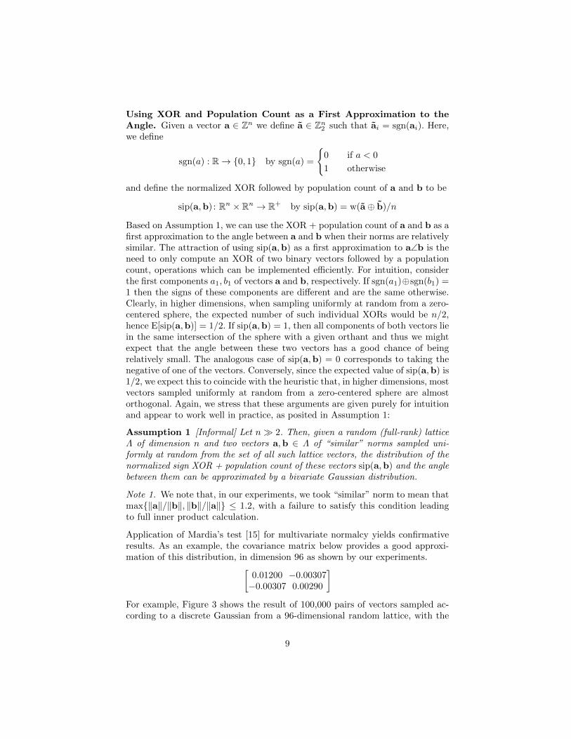
Application of Mardia’s test [15] for multivariate normalcy yields confirmativeresults. As an example, the covariance matrix below provides a good approxi-mation of this distribution, in dimension 96 as shown by our experiments.[

0.01200 −0.00307−0.00307 0.00290

]For example, Figure 3 shows the result of 100,000 pairs of vectors sampled ac-cording to a discrete Gaussian from a 96-dimensional random lattice, with the

9

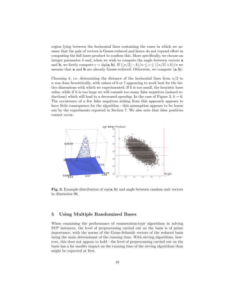
region lying between the horizontal lines containing the cases in which we as-sume that the pair of vectors is Gauss-reduced and hence do not expend effort incomputing the full inner-product to confirm this. More specifically, we choose aninteger parameter k and, when we wish to compute the angle between vectors aand b, we firstly compute c = sip(a,b). If (bn/2c−k)/n ≤ c ≤ (dn/2e+k)/n weassume that a and b are already Gauss-reduced. Otherwise, we compute 〈a,b〉.

Choosing k, i.e. determining the distance of the horizontal lines from n/2 ton was done heuristically, with values of 6 or 7 appearing to work best for the lat-tice dimensions with which we experimented. If k is too small, the heuristic losesvalue, while if it is too large we will commit too many false negatives (missed re-ductions) which will lead to a decreased speedup. In the case of Figure 3, k = 6.The occurrence of a few false negatives arising from this approach appears tohave little consequence for the algorithm - this assumption appears to be borneout by the experiments reported in Section 7. We also note that false positivescannot occur.

Fig. 3. Example distribution of sip(a,b) and angle between random unit vectorsin dimension 96.

5 Using Multiple Randomized Bases

When examining the performance of enumeration-type algorithms in solvingSVP instances, the level of preprocessing carried out on the basis is of primeimportance, with the norms of the Gram-Schmidt vectors of the reduced basisbeing the main determinant of the running time. With sieving algorithms, how-ever, this does not appear to hold - the level of preprocessing carried out on thebasis has a far smaller impact on the running time of the sieving algorithms thanmight be expected at first.

10

We posit that a much more natural consideration is the number of random-ized lattice bases which are reduced and used to “seed” the list. That is, insteadof adding the input basis to the list before starting the sieving procedure, werandomize and reduce the given basis several times, appending all so-obtainedlattice vectors to the list L by running GaussReduce(bi, L,S) for all obtainedvectors bi (cf. Algorithm 1).

The idea of rerandomizing and reducing a given lattice basis for algorith-mic improvements is not new. Indeed, Gama et al. [7] show, with respect toenumeration-based SVP algorithms, a theoretical exponential speedup if the in-put basis is rerandomized, reduced and the enumeration search tree for eachreduced basis is pruned extremely. Experiments confirm this huge speedup inpractice [13]. While in enumeration rerandomizing and reducing provides al-most independent instances of (pruned) enumeration, in this modification toGaussSieve we instead concurrently exploit all the information gathered throughall generated bases in a single instance of GaussSieve rather than running mul-tiple instances of GaussSieve.

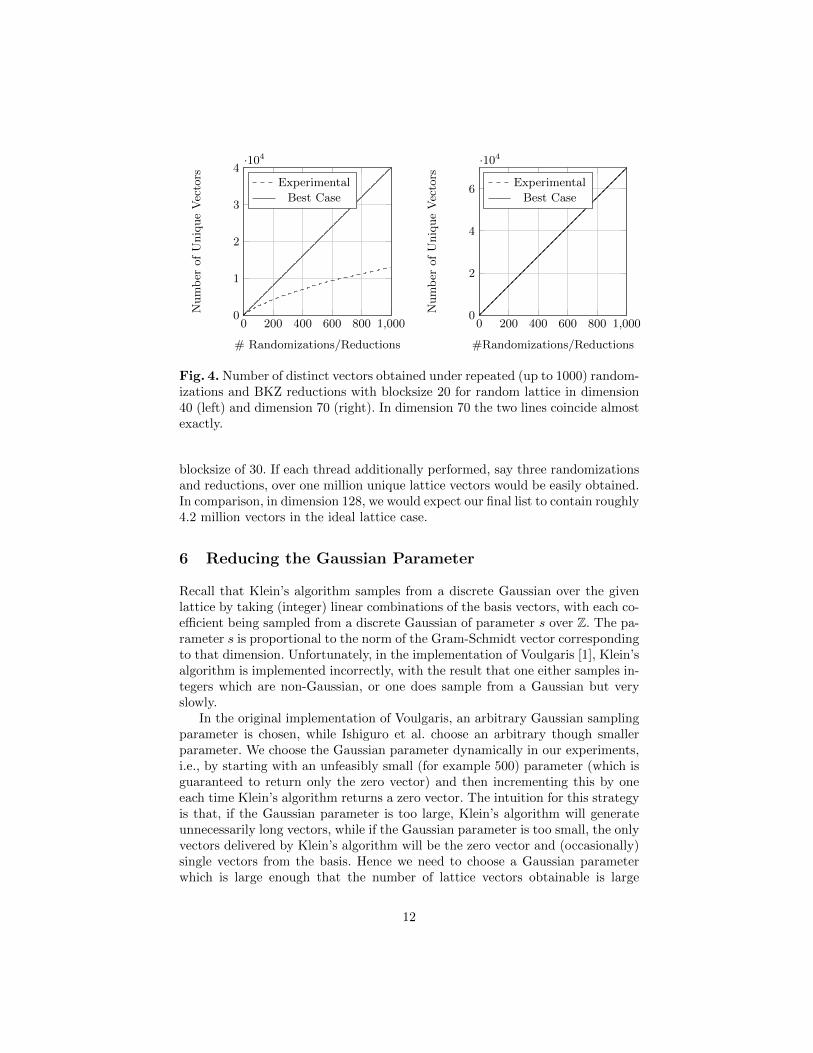
However, a natural concern that arises in this setting is that of the number ofunique lattice vectors we can hope to obtain by way of multiple randomizationand reduction - we wish for this number to be as large as possible to maximizethe size of our starting list. Our experiments indicate that, given a large enoughlattice dimension, the number of duplicate vectors obtained by this approachis negligible even when performing a few thousand such randomizations andreductions. Figure 4 illustrates the number of distinct vectors obtained throughthis approach in dimensions 40 and 70, highlighting that, beyond toy dimensions,obtaining distinct vectors through this approach is not problematic. We alsoobserve that such a “seeding” of the list is only slightly more costly in practiceas this approach makes the first stage of the algorithm embarrassingly parallel,i.e. each thread can carry out an independent basis randomization and reduction,with a relatively fast merging of the resulting collection of vectors into a pairwiseGauss-reduced list.

After seeding the list using the vectors from the reduced bases, we addition-ally store these bases and, rather than sampling all vectors from a single basis,sample from our multiple bases in turn. We note that our optimizations havesome similarities with the random sampling algorithm of Schnorr [23]. Here, shortlattice vectors are sampled to update a given basis, thereby performing multiplelattice reductions. However, we add new vectors into the list while Schnorr’salgorithm uses a fixed number of vectors throughout the execution.

In practice, this modification appears to give linear speedups based on ourexperimental timing results given in Section 7.

Given that parallel adaptations of GaussSieve are highly practical, especiallyfor ideal lattices, we expect the approach of randomizing and reducing the basisto seed the list to be very effective in practice. For instance, the implementationof Ishiguro et al. employed more than 2,688 threads to solve the Ideal-SVP128-dimensional challenge, with the number of thread-hours totaling 479,904.However, only a single basis was used, having been reduced with BKZ with a

11

0 200 400 600 800 1,0000

1

2

3

4·104

# Randomizations/Reductions

Num

ber

of

Uniq

ue

Vec

tors

Experimental

Best Case

0 200 400 600 800 1,0000

2

4

6

·104

#Randomizations/Reductions

Num

ber

of

Uniq

ue

Vec

tors

Experimental

Best Case

Fig. 4. Number of distinct vectors obtained under repeated (up to 1000) random-izations and BKZ reductions with blocksize 20 for random lattice in dimension40 (left) and dimension 70 (right). In dimension 70 the two lines coincide almostexactly.

blocksize of 30. If each thread additionally performed, say three randomizationsand reductions, over one million unique lattice vectors would be easily obtained.In comparison, in dimension 128, we would expect our final list to contain roughly4.2 million vectors in the ideal lattice case.

6 Reducing the Gaussian Parameter

Recall that Klein’s algorithm samples from a discrete Gaussian over the givenlattice by taking (integer) linear combinations of the basis vectors, with each co-efficient being sampled from a discrete Gaussian of parameter s over Z. The pa-rameter s is proportional to the norm of the Gram-Schmidt vector correspondingto that dimension. Unfortunately, in the implementation of Voulgaris [1], Klein’salgorithm is implemented incorrectly, with the result that one either samples in-tegers which are non-Gaussian, or one does sample from a Gaussian but veryslowly.

In the original implementation of Voulgaris, an arbitrary Gaussian samplingparameter is chosen, while Ishiguro et al. choose an arbitrary though smallerparameter. We choose the Gaussian parameter dynamically in our experiments,i.e., by starting with an unfeasibly small (for example 500) parameter (which isguaranteed to return only the zero vector) and then incrementing this by oneeach time Klein’s algorithm returns a zero vector. The intuition for this strategyis that, if the Gaussian parameter is too large, Klein’s algorithm will generateunnecessarily long vectors, while if the Gaussian parameter is too small, the onlyvectors delivered by Klein’s algorithm will be the zero vector and (occasionally)single vectors from the basis. Hence we need to choose a Gaussian parameterwhich is large enough that the number of lattice vectors obtainable is large

12

0 2 4 6 8

·104

0

0.2

0.4

0.6

0.8

1·104

Iteration

Lis

tSiz

e

Optimized Sampling

Implementation-β Sampling

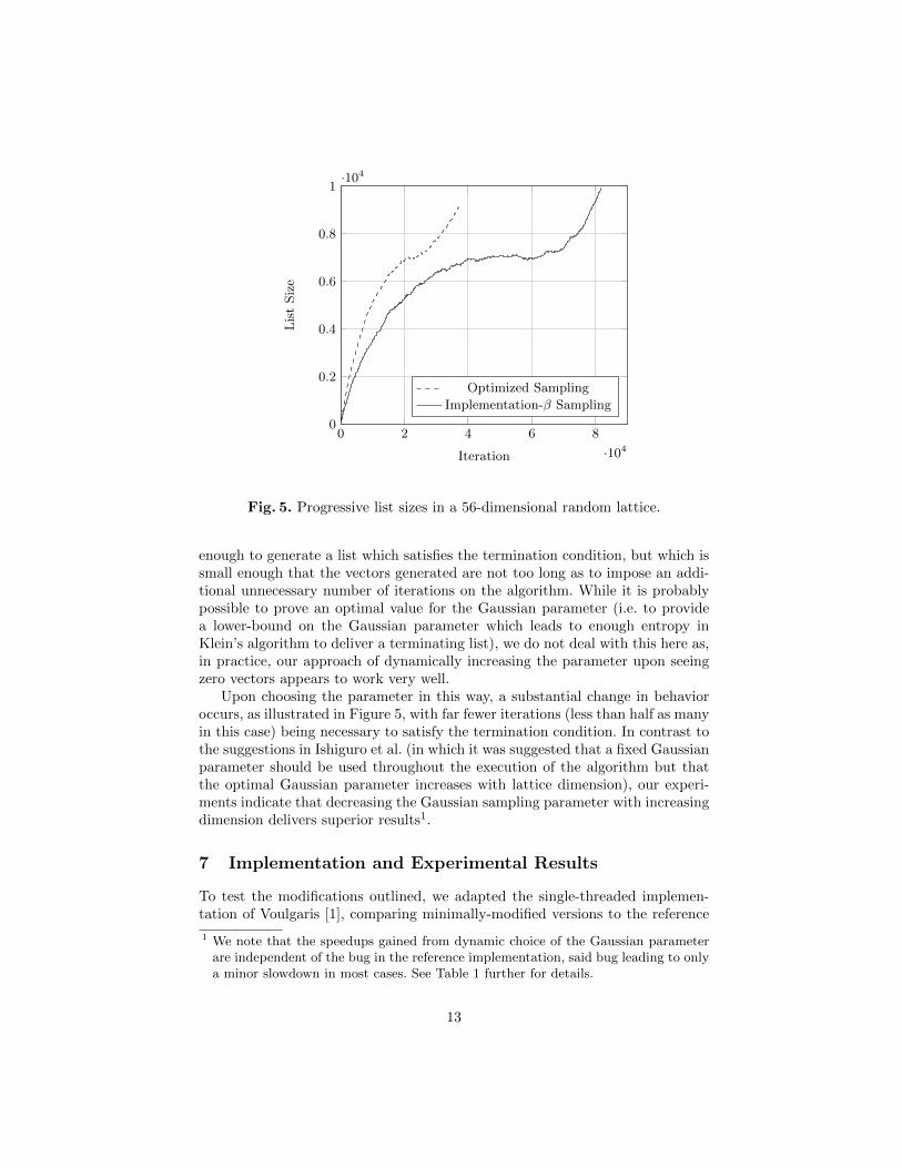
Fig. 5. Progressive list sizes in a 56-dimensional random lattice.

enough to generate a list which satisfies the termination condition, but which issmall enough that the vectors generated are not too long as to impose an addi-tional unnecessary number of iterations on the algorithm. While it is probablypossible to prove an optimal value for the Gaussian parameter (i.e. to providea lower-bound on the Gaussian parameter which leads to enough entropy inKlein’s algorithm to deliver a terminating list), we do not deal with this here as,in practice, our approach of dynamically increasing the parameter upon seeingzero vectors appears to work very well.

Upon choosing the parameter in this way, a substantial change in behavioroccurs, as illustrated in Figure 5, with far fewer iterations (less than half as manyin this case) being necessary to satisfy the termination condition. In contrast tothe suggestions in Ishiguro et al. (in which it was suggested that a fixed Gaussianparameter should be used throughout the execution of the algorithm but thatthe optimal Gaussian parameter increases with lattice dimension), our experi-ments indicate that decreasing the Gaussian sampling parameter with increasingdimension delivers superior results1.

7 Implementation and Experimental Results

To test the modifications outlined, we adapted the single-threaded implemen-tation of Voulgaris [1], comparing minimally-modified versions to the reference

1 We note that the speedups gained from dynamic choice of the Gaussian parameterare independent of the bug in the reference implementation, said bug leading to onlya minor slowdown in most cases. See Table 1 further for details.

13

implementation. While several obvious optimizations are possible, we did not im-plement these, for consistency. We stress, however, that the timings given hereare purely for comparative purposes and in addition to our algorithmic optimiza-tions further optimizations at the implementation level can significantly enhancethe performance of the algorithm, for instance using 16-bit integers for vectorentries rather than the 64-bit integers used in the reference implementation.

All experiments were carried out using a single core of an AMD FX-83504.0GHz CPU, 32GB RAM, with all software (C++) compiled using the GnuCompiler Collection, version 4.7.2-5. Throughout, we only experiment with theGoldstein-Mayer quasi-random lattices as provided by the TU Darmstadt SVPchallenge [2].

7.1 Our Timings

In order to better assess the impact of our modifications to GaussSieve, we com-pare our implementations both to the original implementation of Voulgaris anda “corrected” version where we embed a correct implementation of a discreteGaussian sampler2. We denote the original implementation by “Reference Im-plementation” and the original implementation + corrected Gaussian samplerby “Reference Implementation-β”.

Table 1 shows timings for the original (unoptimized) implementation of Voul-garis [1], of Reference Implementation-β, and of our proposed optimizations ex-plicitly. We also provide timings for an implementation which incorporates all thediscussed optimizations for which the pseudocode can be found in Appendix A.For the multiple-bases optimization we display the timing with best efficiency,i.e., with the optimal (in terms of our limited experiments) number of bases.All timings exclude the cost of lattice reduction but we include the additionalnecessary lattice reduction via BKZ when considering multiple bases.

We observe that our optimized Gaussian sampler gives a speedup of up to3.0x. However, with increasing dimension the speedup decreases slightly. Our in-tegration of approximate inner-product computations increases performance bya factor of up to 2.7x, as compared to the original implementation of GaussSieve.

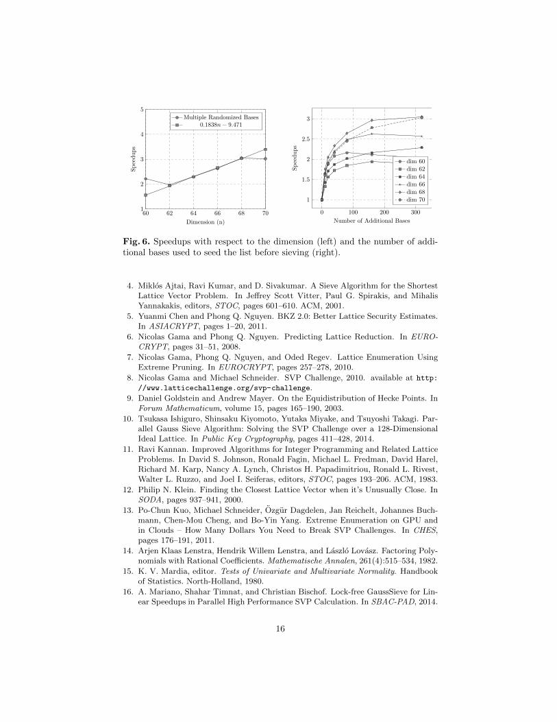
Similar speedups are obtained by considering multiple randomized bases;however, the speedup increases for larger dimensions. Indeed, if we ignore dimen-sion 70, for which we did not consider an optimal number of bases due to timeconstraints, the speedup is approximated closely by the function 0.1838n−9.471.Figure 6 illustrates the speedups for several dimensions when increasing the num-ber of bases considered.

When employing multiple randomized bases it is almost always the case thatwith increasing dimension employing more bases is preferable. Table 2 shows the

2 In the implementation of Voulgaris, no lookup table is employed for Gaussian carry-ing out rejection sampling over a subset of the integers. Hence, the sampled integersare much closer to uniform than to the intended truncated Gaussian. In our cor-rected comparative implementation we employ the same Gaussian parameter fromthe Voulgaris implementation but ensure that the sampled vectors adhere to theprescribed Gaussian.

14

Dimension 60 62 64 66 68 70

Reference Implementation [1] 464 1087 2526 5302 12052 23933

Reference Implementation-β 455 1059 2497 5370 12047 24055

XOR + Pop. Count (Sec. 4) 203 459 1042 2004 4965 11161

Mult. Rand. Bases (Sec. 5) 210 555 1103 2023 3949 7917

Opt. Gaussian Sampling (Sec. 6) 158 376 1023 2222 5389 10207

Combined (s) 79 146 397 868 2082 4500

Shortest Norm ≈ 1943 2092 2103 2099 2141 2143

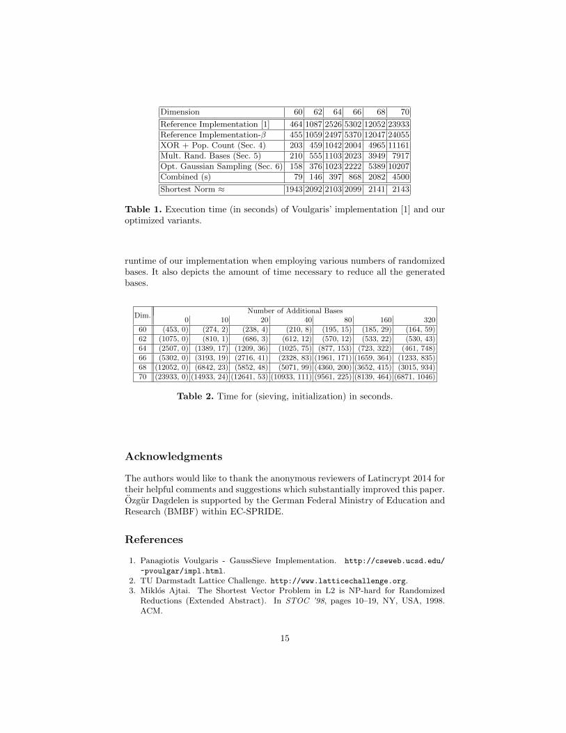
Table 1. Execution time (in seconds) of Voulgaris’ implementation [1] and ouroptimized variants.

runtime of our implementation when employing various numbers of randomizedbases. It also depicts the amount of time necessary to reduce all the generatedbases.

Dim.Number of Additional Bases

0 10 20 40 80 160 320

60 (453, 0) (274, 2) (238, 4) (210, 8) (195, 15) (185, 29) (164, 59)

62 (1075, 0) (810, 1) (686, 3) (612, 12) (570, 12) (533, 22) (530, 43)

64 (2507, 0) (1389, 17) (1209, 36) (1025, 75) (877, 153) (723, 322) (461, 748)

66 (5302, 0) (3193, 19) (2716, 41) (2328, 83) (1961, 171) (1659, 364) (1233, 835)

68 (12052, 0) (6842, 23) (5852, 48) (5071, 99) (4360, 200) (3652, 415) (3015, 934)

70 (23933, 0) (14933, 24) (12641, 53) (10933, 111) (9561, 225) (8139, 464) (6871, 1046)

Table 2. Time for (sieving, initialization) in seconds.

Acknowledgments

The authors would like to thank the anonymous reviewers of Latincrypt 2014 fortheir helpful comments and suggestions which substantially improved this paper.Ozgur Dagdelen is supported by the German Federal Ministry of Education andResearch (BMBF) within EC-SPRIDE.

References

1. Panagiotis Voulgaris - GaussSieve Implementation. http://cseweb.ucsd.edu/

~pvoulgar/impl.html.2. TU Darmstadt Lattice Challenge. http://www.latticechallenge.org.3. Miklos Ajtai. The Shortest Vector Problem in L2 is NP-hard for Randomized

Reductions (Extended Abstract). In STOC ’98, pages 10–19, NY, USA, 1998.ACM.

15

60 62 64 66 68 701

2

3

4

5

Dimension (n)

Speedups

Multiple Randomized Bases0.1838n− 9.471

0 100 200 300

1

1.5

2

2.5

3

Number of Additional Bases

Speedups

dim 60dim 62dim 64dim 66dim 68dim 70

Fig. 6. Speedups with respect to the dimension (left) and the number of addi-tional bases used to seed the list before sieving (right).

4. Miklos Ajtai, Ravi Kumar, and D. Sivakumar. A Sieve Algorithm for the ShortestLattice Vector Problem. In Jeffrey Scott Vitter, Paul G. Spirakis, and MihalisYannakakis, editors, STOC, pages 601–610. ACM, 2001.

5. Yuanmi Chen and Phong Q. Nguyen. BKZ 2.0: Better Lattice Security Estimates.In ASIACRYPT, pages 1–20, 2011.

6. Nicolas Gama and Phong Q. Nguyen. Predicting Lattice Reduction. In EURO-CRYPT, pages 31–51, 2008.

7. Nicolas Gama, Phong Q. Nguyen, and Oded Regev. Lattice Enumeration UsingExtreme Pruning. In EUROCRYPT, pages 257–278, 2010.

8. Nicolas Gama and Michael Schneider. SVP Challenge, 2010. available at http:

//www.latticechallenge.org/svp-challenge.

9. Daniel Goldstein and Andrew Mayer. On the Equidistribution of Hecke Points. InForum Mathematicum, volume 15, pages 165–190, 2003.

10. Tsukasa Ishiguro, Shinsaku Kiyomoto, Yutaka Miyake, and Tsuyoshi Takagi. Par-allel Gauss Sieve Algorithm: Solving the SVP Challenge over a 128-DimensionalIdeal Lattice. In Public Key Cryptography, pages 411–428, 2014.

11. Ravi Kannan. Improved Algorithms for Integer Programming and Related LatticeProblems. In David S. Johnson, Ronald Fagin, Michael L. Fredman, David Harel,Richard M. Karp, Nancy A. Lynch, Christos H. Papadimitriou, Ronald L. Rivest,Walter L. Ruzzo, and Joel I. Seiferas, editors, STOC, pages 193–206. ACM, 1983.

12. Philip N. Klein. Finding the Closest Lattice Vector when it’s Unusually Close. InSODA, pages 937–941, 2000.

13. Po-Chun Kuo, Michael Schneider, Ozgur Dagdelen, Jan Reichelt, Johannes Buch-mann, Chen-Mou Cheng, and Bo-Yin Yang. Extreme Enumeration on GPU andin Clouds – How Many Dollars You Need to Break SVP Challenges. In CHES,pages 176–191, 2011.

14. Arjen Klaas Lenstra, Hendrik Willem Lenstra, and Laszlo Lovasz. Factoring Poly-nomials with Rational Coefficients. Mathematische Annalen, 261(4):515–534, 1982.

15. K. V. Mardia, editor. Tests of Univariate and Multivariate Normality. Handbookof Statistics. North-Holland, 1980.

16. A. Mariano, Shahar Timnat, and Christian Bischof. Lock-free GaussSieve for Lin-ear Speedups in Parallel High Performance SVP Calculation. In SBAC-PAD, 2014.

16

17. D. Micciancio and S. Goldwasser. Complexity of Lattice Problems: A CryptographicPerspective. Milken Institute Series on Financial Innovation and Economic Growth.Springer US, 2002.

18. Daniele Micciancio and Panagiotis Voulgaris. Faster Exponential Time Algorithmsfor the Shortest Vector Problem. In Proceedings of the Twenty-first Annual ACM-SIAM Symposium on Discrete Algorithms, SODA ’10, pages 1468–1480. Societyfor Industrial and Applied Mathematics, 2010.

19. Benjamin Milde and Michael Schneider. A Parallel Implementation of GaussSievefor the Shortest Vector Problem in Lattices. In Victor Malyshkin, editor, PaCT,volume 6873 of Lecture Notes in Computer Science, pages 452–458. Springer, 2011.

20. Phong Q. Nguyen and Thomas Vidick. Sieve Algorithms for the Shortest VectorProblem are Practical. J. Mathematical Cryptology, 2(2):181–207, 2008.

21. Michael Schneider. Sieving for Shortest Vectors in Ideal Lattices. IACR CryptologyePrint Archive, 2011:458, 2011.

22. Claus-Peter Schnorr. A Hierarchy of Polynomial Time Lattice Basis ReductionAlgorithms. Theor. Comput. Sci., 53:201–224, 1987.

23. Claus-Peter Schnorr. Lattice Reduction by Random Sampling and Birthday Meth-ods. In STACS, pages 145–156, 2003.

24. Carl Ludwig Siegel. A mean value theorem in geometry of numbers. Annals ofMathematics, 46(2), 1945.

25. Brigitte Vallee and Antonio Vera. Probabilistic Analyses of Lattice ReductionAlgorithms. In Phong Q. Nguyen and Brigitte Vallee, editors, The LLL Algorithm,Information Security and Cryptography, pages 71–143. Springer, 2010.

26. Xiaoyun Wang, Mingjie Liu, Chengliang Tian, and Jingguo Bi. Improved Nguyen-Vidick heuristic sieve algorithm for shortest vector problem. In ASIACCS, pages1–9, 2011.

27. Feng Zhang, Yanbin Pan, and Gengran Hu. A Three-Level Sieve Algorithm for theShortest Vector Problem. In Selected Areas in Cryptography, pages 29–47, 2013.

A Pseudocode of our Optimized GaussSieve

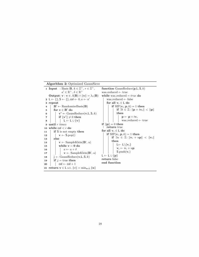
The below pseudocode displays our proposed modifications to GaussSieve. Inlines (3)-(9) we incorporate our multiple-randomized-bases optimization, and inthe function GaussReduce(p,L,S, k) we embed the cheap test SIP implementingour XOR + population count computation for the approximation of the anglebetween two vectors. The optimized Gaussian sampler modifies the functionSampleKlein.

In the pseudocode, the parameter k ∈ Z+ defines the bounds on the XOR+ population count, within which we assume that a pair of vectors is Gauss-reduced, i.e. if n/2 − k ≤ 〈a, b〉 ≤ n/2 + k, we assume the pair a,b are Gauss-reduced.

17

Algorithm 2: Optimized GaussSieve

1 Input : Basis B, k ∈ Z+, r ∈ Z+,a′ ∈ R+, δ ∈ R+

Output: v : v ∈ Λ(B) ∧ ‖v‖ = λ1(B)2 L← {}, S← {}, col← 0, a← a′

3 repeat4 B′ ← RandomizeBasis(B)5 for v ∈ B′ do6 v’ ← GaussReduce(v,L, S, k)7 if ‖v′‖ 6= 0 then8 L← L ∪ {v}9 until r times

10 while col < c do11 if S is not empty then12 v ← S.pop()13 else14 v ← SampleKlein(B’, a)15 while v = 0 do16 a← a+ δ17 v ← SampleKlein(B’, a)

18 j ← GaussReduce(v,L,S, k)19 if j = true then20 col← col + 1

21 return v ∈ L s.t. ‖v‖ = minx∈L ‖x‖

function GaussReduce(p,L, S, k)was reduced← truewhile was reduced = true do

was reduced← falsefor all vi ∈ L do

if SIP(vi,p, k) = 1 thenif ∃t ∈ Z : ‖p + tvi‖ < ‖p‖then

p← p + tvi

was reduced← true

if ‖p‖ = 0 thenreturn true

for all vi ∈ L doif SIP(vi,p, k) = 1 then

if ∃u ∈ Z : ‖vi + up‖ < ‖vi‖then

L← L\{vi}vi ← vi + upS.push(vi)

L← L ∪ {p}return falseend function

18