truncated gaussian and plurigaussian ......truncated gaussian and plurigaussian simulations of...

TRUNCATED GAUSSIAN AND PLURIGAUSSIAN

SIMULATIONS OF LITHOLOGICAL UNITS IN MANSA

MINA DEPOSIT RODRIGO RIQUELME T1, GAËLLE LE LOC’H2 and PEDRO CARRASCO C.1 1

CODELCO, Santiago, Chile 2 Geostatistics team, Geosciences centre, MINES ParisTech, Fontainebleau, France

ABSTRACT

Mansa Mina orebody is a porphyry copper orebody, satellite of Chuquicamata

copper mine, where the erosion and weathering have not yet masked or removed

too much of the lithological units describing the copper enrichment process. This

enrichment process, due to fluids guided by the fracturation network leads to a

mineralization geometry sub-parallel to Mansa Mina fault. A previous feasibility

study has shown few years ago that the Truncated Gaussian method could be

useful for the simulation of its geological units. Truncated Gaussian simulations

have been conducted again with more care, after addition of more data. As the

simultaneous modelling of all these units with the same underlying Gaussian

random function is not completely satisfactory, Plurigaussian simulations have

then been conducted and present better results, consistent with the geological

block model. 16 Plurigaussian simulations have then been used to get a first

evaluation of the uncertainties on the ore volume in the pit corresponding to the

first five years of production.

GENERAL PRESENTATION OF THE CASE STUDY

Brief Geological Description

Mansa Mina (MM) is a mining project on a porphyry copper orebody, satellite of Chuquicamata mine. The purpose of the present study is to simulate, before the opening of the mine, the “geological units”, which control the copper grade distribution in space. The mineralization of MM deposit is controlled by fracturation and joint network associated with the MM fault. MM fault has a global North-South sub-vertical orientation, but it slightly curves in the studied area. The geological units, defined from geological criteria, describe the mineralization events and control the grade distribution in the orebody.

R. RIQUELME TAPIA, G. LE LOC’H AND P. CARRASCO

GEOSTATS 2008, Santiago, Chile

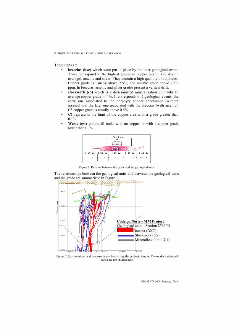
These units are: • breccias (bxc) which were put in place by the later geological event.

These correspond to the highest grades in copper (about 3 to 4% on average), arsenic and silver. They contain a high quantity of sulphides. Copper grade is usually above 2.5%, and arsenic grade above 2000 ppm. In breccias, arsenic and silver grades present a vertical drift.

• stockwork (c5) which is a disseminated mineralization unit with an average copper grade of 1%. It corresponds to 2 geological events, the early one associated to the porphyry copper appearance (without arsenic) and the later one associated with the breccias (with arsenic). C5 copper grade is usually above 0.5%.

• C1 represents the limit of the copper area with a grade greater than 0.1%

• Waste (est) groups all rocks with no copper or with a copper grade lower than 0.1%.

Figure 1: Relation between the grade and the geological units.

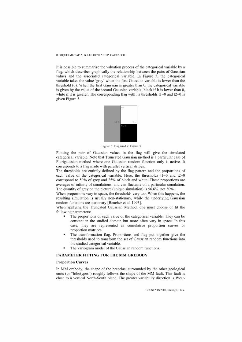
The relationships between the geological units and between the geological units and the grade are summarized in Figure 1

Figure 2: East-West vertical cross-section schematizing the geological units. The oxides and mixed zones are not studied here.

Ele

vati

on

Codelco Norte - MM Project Geological units - Section 25600N Breccia (BXC)

Stockwork (C5)

Mineralized limit (C1)

TRUNCATED GAUSSIAN AND PLURIGAUSSIAN SIMULATIONS OF LITHOLOGICAL UNITS

VIII International Geostatistics Congress

The geometry of these geological units follows more or less the geometry of the fracturation network. Figure 2 shows an East-West vertical cross-section which schematizes this geometry.

Data Presentation

Figure 3: map of drill holes with their geometrical relationships with the MM fault and the breccias.

The data combine two exploration galleries and 496 drill holes which can start from the ground or from the galleries. The drilling is designed to cross as best as possible the fracturation system: deviated drill holes are approximately contained in East-West vertical planes. Figure 3 shows the projection of the drill holes on a horizontal map (left part) and the geometrical relations between the galleries, the drill holes, the MM fault and the sub-vertical breccias.

THE PLURIGAUSSIAN METHOD

The Plurigaussian simulation method is used to simulate categorical variables (for example, lithologies or geological units in MM case). Figure 4 shows the principle of the method [Armstrong et al., 2003]. Two Gaussian random functions are simulated (a and b), then the categorical variable is defined accordingly to the Gaussian values (c).

-3

-3

-2 -2

-2

-1

-1

-1

-1

0 0

0

0

0

0 0 0

111

11

1

1

1

1

2

2

a)

-2

-2

-2

-2

-2

-2

-1

-1-1

-1-1

-1

-1

-1

00

0 00

00

0

00

0

00

0

0 0

11

1 11

b) c)

Figure 4: principle of the Plurigaussian simulation method. a) First Gaussian random function; b) second Gaussian random function; c) resulting categorical variable.

MM fault



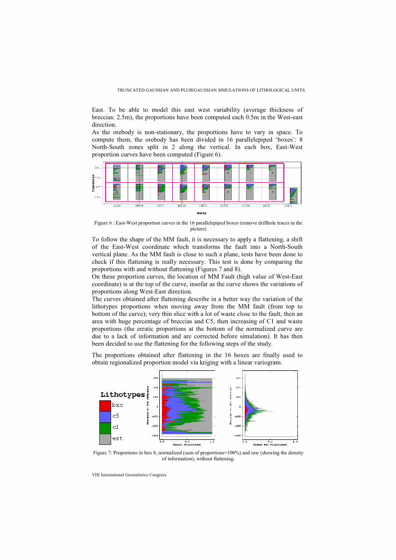
It is possible to summarize the valuation process of the categorical variable by a flag, which describes graphically the relationship between the pairs of Gaussian values and the associated categorical variable. In Figure 3, the categorical variable takes the value ‘grey’ when the first Gaussian variable is lower than the threshold (0). When the first Gaussian is greater than 0, the categorical variable is given by the value of the second Gaussian variable: black if it is lower than 0, white if it is greater. The corresponding flag with its thresholds t1=0 and t2=0 is given Figure 5.

G1

G2

t2=0

t1=0

Figure 5: Flag used in Figure 3

Plotting the pair of Gaussian values in the flag will give the simulated categorical variable. Note that Truncated Gaussian method is a particular case of Plurigaussian method where one Gaussian random function only is active. It corresponds to a flag made with parallel vertical stripes. The thresholds are entirely defined by the flag pattern and the proportions of each value of the categorical variable. Here, the thresholds t1=0 and t2=0 correspond to 50% of grey and 25% of black and white. These proportions are averages of infinity of simulations, and can fluctuate on a particular simulation. The quantity of grey on the picture (unique simulation) is 56.6%, not 50%. When proportions vary in space, the thresholds vary too. When this happens, the resulting simulation is usually non-stationary, while the underlying Gaussian random functions are stationary [Beucher et al. 1993]. When applying the Truncated Gaussian Method, one must choose or fit the following parameters:

� The proportions of each value of the categorical variable. They can be constant in the studied domain but more often vary in space. In this case, they are represented as cumulative proportion curves or proportion matrices.

� The transformation flag. Proportions and flag put together give the thresholds used to transform the set of Gaussian random functions into the studied categorical variable.

� The variogram model of the Gaussian random functions.

PARAMETER FITTING FOR THE MM OREBODY

Proportion Curves

In MM orebody, the shape of the breccias, surrounded by the other geological units (or “lithotypes”) roughly follows the shape of the MM fault. This fault is close to a vertical North-South plane. The greater variability direction is West-



East. To be able to model this east west variability (average thickness of breccias: 2.5m), the proportions have been computed each 0.5m in the West-east direction. As the orebody is non-stationary, the proportions have to vary in space. To compute them, the orebody has been divided in 16 parallelepiped ‘boxes’: 8 North-South zones split in 2 along the vertical. In each box, East-West proportion curves have been computed (Figure 6).

Figure 6 : East-West proportion curves in the 16 parallelepiped boxes (remove drillhole traces in the picture)

To follow the shape of the MM fault, it is necessary to apply a flattening, a shift of the East-West coordinate which transforms the fault into a North-South vertical plane. As the MM fault is close to such a plane, tests have been done to check if this flattening is really necessary. This test is done by comparing the proportions with and without flattening (Figures 7 and 8). On these proportion curves, the location of MM Fault (high value of West-East coordinate) is at the top of the curve, insofar as the curve shows the variations of proportions along West-East direction. The curves obtained after flattening describe in a better way the variation of the lithotypes proportions when moving away from the MM fault (from top to bottom of the curve); very thin slice with a lot of waste close to the fault, then an area with huge percentage of breccias and C5, then increasing of C1 and waste proportions (the erratic proportions at the bottom of the normalized curve are due to a lack of information and are corrected before simulation). It has then been decided to use the flattening for the following steps of the study.

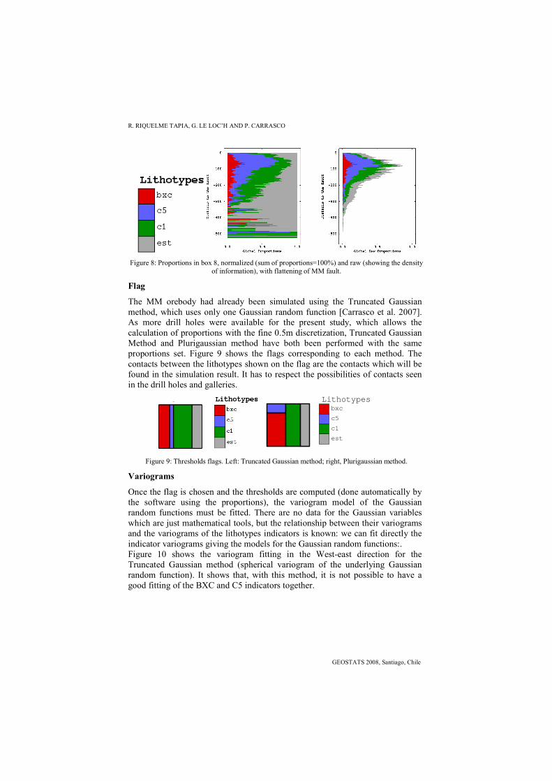
The proportions obtained after flattening in the 16 boxes are finally used to obtain regionalized proportion model via kriging with a linear variogram.

Figure 7: Proportions in box 8, normalized (sum of proportions=100%) and raw (showing the density of information), without flattening.



Figure 8: Proportions in box 8, normalized (sum of proportions=100%) and raw (showing the density of information), with flattening of MM fault.

Flag

The MM orebody had already been simulated using the Truncated Gaussian method, which uses only one Gaussian random function [Carrasco et al. 2007]. As more drill holes were available for the present study, which allows the calculation of proportions with the fine 0.5m discretization, Truncated Gaussian Method and Plurigaussian method have both been performed with the same proportions set. Figure 9 shows the flags corresponding to each method. The contacts between the lithotypes shown on the flag are the contacts which will be found in the simulation result. It has to respect the possibilities of contacts seen in the drill holes and galleries.

DrapeauDrapeau Lithotypesbxc

c5

c1

est

Drapeau Lithotypesbxc

c5

c1

est

Drapeau

Figure 9: Thresholds flags. Left: Truncated Gaussian method; right, Plurigaussian method.

Variograms

Once the flag is chosen and the thresholds are computed (done automatically by the software using the proportions), the variogram model of the Gaussian random functions must be fitted. There are no data for the Gaussian variables which are just mathematical tools, but the relationship between their variograms and the variograms of the lithotypes indicators is known: we can fit directly the indicator variograms giving the models for the Gaussian random functions:. Figure 10 shows the variogram fitting in the West-east direction for the Truncated Gaussian method (spherical variogram of the underlying Gaussian random function). It shows that, with this method, it is not possible to have a good fitting of the BXC and C5 indicators together.



Figure 10: Indicator variogram fitting for the Truncated Gaussian method in the West-East direction. Left: West-East range 7m; right: West-east range 20m.

Finally, for the Truncated Gaussian method, two variograms models will be tested. The first model is spherical, with ranges 120m, 70m and 7m in NS, vertical and W-E directions. The second model is identical except for the 20m range in the W-E direction.

Figure 11: Indicator variograms fitting for the Plurigaussian method, in the 3 coordinate directions (a: North-South; b: vertical; c: West-east).

The plurigaussian method gives more freedom in the variogram fitting, and it should be easier to fit all indicators together with this method. Figure 11 shows



the final fitting of the lithotype indicator variograms in the directions of the 3 coordinates. The fitted models are:

• for the first Gaussian random function, an exponential model with range 100m in the North-South direction, 80m in the vertical direction and 25m in the West-East direction

• for the second Gaussian random function, a spherical model with range 25m in the North-South direction, 40m in the vertical direction and 5m in the West-East direction

In some cases (Figure 11c) there can be a discrepancy between the sill of the experimental variogram and the sill of the model. The reason is because the sills are entirely controlled by the proportions. In non-stationary cases as here, poorly sampled areas and highly sampled areas (where the proportions are usually not the same) have the same influence on the overall variogram model, while it is obviously not the case for the experimental variogram.

SIMULATIONS

Figure 12 shows a horizontal section of two Truncated Gaussian simulations, one for each model. The simulation with the W-E range 7m shows a C5 unit which is not continuous enough, while the simulation with the 20m W-E range gives too much continuity to the breccias.

Figure 12: comparison of Truncated Gaussian simulations with different W-E ranges. Left: range 7m; right: range 20m.

For the Plurigaussian method, 46 simulations have been performed with the same data. Figure 13 compares 3 horizontal sections on the same level: two different simulations and the block model drawn by the geologist without the use of geostatistics (waste unit is plotted in white). While these 3 sections are obviously different, Plurigaussian simulations are a lot more consistent with the



block model designed by the geologist than the Truncated Gaussian simulations. It is probably due to the higher flexibility which allows a better fit of the model.

Figure13: Comparison between 2 simulations (left and centre) and the block model of may 2006 (right)

ORE TONNAGE EVALUATION AND CONCLUSION

Table 1 shows the mix of the geological units expected by the mine plan of the 5 first years of production.

Table 1: Planned mix for the five first years of production

Geological units BXC C5 C1 est Total

Tonnage 17% 57% 21% 4% 100% Copper Tonnage 50% 47% 3% 100%

Table 2 shows statistics (average, standard and relative variability -2 standard deviations given as a percentage of the average values) of the global estimation of the volume (ore tonnage given in number of blocks) for the high and middle grade geological units BXC and C5 for the 46 simulations, in the domain to be mined in these 5 first years.



Table 2: Statistics on the breccias and C5 volume over the 46 simulations.

Block number Percentage BXC C5 bxc+c5 BXC C5 bxc+c5

Average 257,968 827,371 1,085,340 9.04% 28.99% 38.03%

Standard deviation

3,572 9,374 12,466 0.14% 0.33% 0.44%

Relative variability

2.77% 2.27% 2.30% 2.77% 2.27% 2.30%

While C1 is not a waste unit, its grade is low and it will only been mined in association with BXC and C5. The mine plan is based on BXC + C5. Although plurigaussian simulations are close to the initial block model, their variability gives an idea of the uncertainty in the tonnage, and can be used to evaluate a part of the risk associated with the mine plan. In MM case, the global variability shown by the simulation set is very low (2.30% for BXC + C5). This means that for the 5 first years of production, the sampling density is sufficient for mine planning purpose. In conclusion, the Plurigaussian method has allowed modelling the geological units spatial distribution, consistently with the known geometric control of the MM fault and with a better fit of the BXC and C5 variability than the truncated Gaussian method. The resultant simulations are quite close to the geological model, which confirms the applicability of the method in our case. By allowing performing simulation, it has the advantage to provide statistics on the global variability of the model, statistics which have a huge importance in mine planning before the beginning of the production.

ACKNOWLEDGEMENTS

The authors thank to Fernando Vivanco Giesen, Julio Beniscelli Troncoso & Roberto Fréraut Contreras of CODELCO for providing the data & help for development of the CFSG project. The present study represents a part of this project. REFERENCES

Armstrong M., Galli A., Geffroy, F., Le Loc’h G., Eschard R. 2003. Plurigaussian Simulations in Geosciences. Springer Verlag, Berlin Heidelberg

Beucher H., Galli A., Le Loc’h G., Ravenne C., Heresim Group. 1993. Including a regional trend in reservoir modelling using the Truncated Gaussian method. In Soares ed., Geostatistics Tróia ’92. Vol. 1. Dordrecht: Kluwer. Pp.555-566.

Carrasco, P., Carrasco, P., Ibarra, F., Rojas, R. Le Loc’h, G., Seguret, S. (2007) Application of the Truncated Gaussian simulation method to a porphyry copper deposit. In Magri ed., APCOM 2007, 33rd International Symposium on Application of Computers and Operations research in the Mineral industry, pp 31-39

truncated gaussian and plurigaussian ......truncated gaussian and plurigaussian simulations of...

Documents