Atmos. Chem. Phys. Discuss., 6, 2965–3047, 2006www.atmos-chem-phys-discuss.net/6/2965/2006/© Author(s) 2006. This work is licensedunder a Creative Commons License.

AtmosphericChemistry

and PhysicsDiscussions

Multi-model ensemble simulations oftropospheric NO2 compared with GOMEretrievals for the year 2000T. P. C. van Noije1, H. J. Eskes1, F. J. Dentener2, D. S. Stevenson3, K. Ellingsen4,M. G. Schultz5, O. Wild6,7, M. Amann8, C. S. Atherton9, D. J. Bergmann9, I. Bey10,K. F. Boersma1, T. Butler11, J. Cofala8, J. Drevet10, A. M. Fiore12, M. Gauss4,D. A. Hauglustaine13, L. W. Horowitz12, I. S. A. Isaksen4, M. C. Krol2,14,J.-F. Lamarque15, M. G. Lawrence11, R. V. Martin16,17, V. Montanaro18,J.-F. Muller19, G. Pitari18, M. J. Prather20, J. A. Pyle7, A. Richter21,J. M. Rodriguez22, N. H. Savage7, S. E. Strahan22, K. Sudo6, S. Szopa13, andM. van Roozendael19

1Royal Netherlands Meteorological Institute, De Bilt, The Netherlands2Joint Research Centre, Institute for Environment and Sustainability, Ispra, Italy3University of Edinburgh, School of Geosciences, Edinburgh, UK4University of Oslo, Department of Geosciences, Oslo, Norway5Max Planck Institute for Meteorology, Hamburg, Germany6Frontier Research Center for Global Change, JAMSTEC, Yokohama, Japan7University of Cambridge, Centre for Atmospheric Science, UK8International Institute for Applied Systems Analysis, Laxenburg, Austria9Lawrence Livermore National Laboratory, Atmospheric Science Division, Livermore, USA

2965

10 Ecole Polytechnique Federal de Lausanne, Switzerland11 Max Planck Institute for Chemistry, Mainz, Germany12 Geophysical Fluid Dynamics Laboratory, NOAA, Princeton, New Jersey, USA13 Laboratoire des Sciences du Climat et de l’Environnement, Gif-sur-Yvette, France14 Space Research Organisation Netherlands, Utrecht, The Netherlands15 National Center of Atmospheric Research, Atmospheric Chemistry Division, Boulder, Col-orado, USA16 Department of Physics and Atmospheric Science, Dalhousie University, Halifax, Nova Sco-tia, Canada17 Smithsonian Astrophysical Observatory, Cambridge, Massachusetts, USA18 Universita L’Aquila, Dipartimento di Fisica, L’Aquila, Italy19 Belgian Institute for Space Aeronomy, Brussels, Belgium20 Department of Earth System Science, University of California, Irvine, USA21 Institute of Environmental Physics, University of Bremen, Bremen, Germany22 Goddard Earth Sciences and Technology Center, Maryland, Washington, DC, USA

Received: 16 December 2005 – Accepted: 23 January 2006 – Published: 12 April 2006

Correspondence to: T. P. C. van Noije (noije@knmi.nl)

2966

Abstract

We present a systematic comparison of tropospheric NO2 from 17 global atmosphericchemistry models with three state-of-the-art retrievals from the Global Ozone Monitor-ing Experiment (GOME) for the year 2000. The models used constant anthropogenicemissions from IIASA/EDGAR3.2 and monthly emissions from biomass burning based5

on the 1997–2002 average carbon emissions from the Global Fire Emissions Database(GFED). Model output is analyzed at 10:30 local time, close to the overpass time of theERS-2 satellite, and collocated with the measurements to account for sampling bi-ases due to incomplete spatiotemporal coverage of the instrument. We assessed theimportance of different contributions to the sampling bias: correlations on seasonal10

time scale give rise to a positive bias of 30–50% in the retrieved annual means overregions dominated by emissions from biomass burning. Over the industrial regionsof the eastern United States, Europe and eastern China the retrieved annual meanshave a negative bias with significant contributions (between –25% and +10% of theNO2 column) resulting from correlations on time scales from a day to a month. We15

present global maps of modeled and retrieved annual mean NO2 column densities,together with the corresponding ensemble means and standard deviations for modelsand retrievals. The spatial correlation between the individual models and retrievals arehigh, typically in the range 0.81–0.93 after smoothing the data to a common resolution.On average the models underestimate the retrievals in industrial regions, especially20

over eastern China and over the Highveld region of South Africa, and overestimatethe retrievals in regions dominated by biomass burning during the dry season. Thediscrepancy over South America south of the Amazon disappears when we use theGFED emissions specific to the year 2000. The seasonal cycle is analyzed in detailfor eight different continental regions. Over regions dominated by biomass burning,25

the timing of the seasonal cycle is generally well reproduced by the models. However,over Central Africa south of the Equator the models peak one to two months earlierthan the retrievals. We further evaluate a recent proposal to reduce the NOx emission

2967

factors for savanna fires by 40% and find that this leads to an improvement of the am-plitude of the seasonal cycle over the biomass burning regions of Northern and CentralAfrica. In these regions the models tend to underestimate the retrievals during the wetseason, suggesting that the soil emissions are higher than assumed in the models. Ingeneral, the discrepancies between models and retrievals cannot be explained by a5

priori profile assumptions made in the retrievals, neither by diurnal variations in anthro-pogenic emissions, which lead to a marginal reduction of the NO2 abundance at 10:30local time (by 2.5–4.1% over Europe). Overall, there are significant differences amongthe various models and, in particular, among the three retrievals. The discrepanciesamong the retrievals (10–50% in the annual mean over polluted regions) indicate that10

the previously estimated retrieval uncertainties have a large systematic component.Our findings imply that top-down estimations of NOx emissions from satellite retrievalsof tropospheric NO2 are strongly dependent on the choice of model and retrieval.

1 Introduction

Nitrogen dioxide (NO2) plays a key role in tropospheric chemistry with important im-15

plications for air quality and climate change. On the one hand, tropospheric NO2 isessential for maintaining the oxidizing capacity of the atmosphere. Photolysis of NO2during daytime is the major source of ozone (O3) in the troposphere and photolysisof O3 in turn initializes the production of the hydroxyl radical (OH), the main cleans-ing agent of the atmosphere. On the other hand, NO2 as well as O3 are toxic to the20

biosphere and may cause respiratory problems for humans. Moreover, NO2 may re-act with OH to form nitric acid (HNO3), one of the main components of acid rain. Asa greenhouse gas, NO2 contributes significantly to radiative forcing over industrial re-gions, especially in urban areas (Solomon et al., 1999; Velders et al., 2001). Althoughthe direct contribution of tropospheric NO2 to global warming is relatively small, emis-25

sions of nitrogen oxides (NOx≡NO+NO2) affect the global climate indirectly by perturb-ing O3 and methane (CH4) concentrations. Overall, indirect long-term global radiative

2968

cooling due to decreases in CH4 and O3 dominates short-term warming from regionalO3 increases (Wild et al., 2001; Derwent et al., 2001; Berntsen et al., 2005).

The main sources of tropospheric NOx are emissions from fossil fuel combustion,mostly from power generation, road transport as well as marine shipping, and in-dustry. Other important surface sources are emissions from biomass burning, mostly5

from savanna fires and tropical agriculture, and from microbial activity in soils; impor-tant sources in the free troposphere are emissions from lightning and aircraft. Minorsources are due to oxidation of ammonia (NH3) by the biosphere and transport fromthe stratosphere. By far the majority of the NOx is emitted as NO, but photochemicalequilibration with NO2 takes place within a few minutes. The principal sink of tropo-10

spheric NOx is oxidation to HNO3 by reaction of NO2 with OH during daytime and byreaction of NO2 with O3 followed by hydrolysis of N2O5 on aerosols at night (Dentenerand Crutzen, 1993; Evans and Jacob, 2005). The resulting NOx lifetime in the planetaryboundary layer varies from several hours in the tropics to 1–2 days in the extratropicsduring winter (Martin et al., 2003b) and increases to a few days in the upper tropo-15

sphere. Long-range transport of NOx may take place in the form of peroxyacetylnitrate(PAN), which is formed by photochemical oxidation of hydrocarbons in the presenceof NOx. As PAN is stable at low temperatures, it may be transported over large dis-tances through the middle and upper troposphere and release NOx far from its sourceby thermal decomposition during subsidence.20

Because of the relatively heterogeneous distribution of its sources and sinks in com-bination with its short lifetime, the concentration of tropospheric NOx is highly variablein space and time. Monitoring of NO2 therefore requires covering a broad spectrum ofspatial and temporal scales, using a combination of ground-based, air-borne as wellas satellite measurements. During the last decade, observations from space have pro-25

vided a wealth of information on the global and regional distribution of NO2 on daily tomulti-annual time scales. We now have nearly 10 years of tropospheric NO2 data fromthe Global Ozone Monitoring Experiment (GOME) instrument on board the second Eu-ropean Remote Sensing (ERS-2) satellite, which was launched by the European Space

2969

Agency (ESA) in April 1995. ERS-2 flies in a sun-synchronous polar orbit, crossing theequator at 10:30 local time. GOME is a nadir-viewing spectrometer operating in theultraviolet and visible part of the spectrum, and has a forward-scan ground pixel sizeof 320 km across track by 40 km along track. Global coverage of the observations isreached within three days. Global tropospheric NO2 columns have been retrieved from5

GOME for the period January 1996–June 2003; since 22 June 2003 data coverage islimited to Europe, the North Atlantic, western North America, and the Arctic (due tofailure of the ERS-2 tape recorder). Higher resolution tropospheric NO2 retrieval datahave recently become available from the Scanning Imaging Absorption Spectrometerfor Atmospheric Chartography (SCIAMACHY) instrument on board the ESA Envisat10

satellite (launched in March 2002) and from the Ozone Monitoring Instrument (OMI) onboard the NASA Earth Observing System (EOS) Aura satellite (launched in July 2004).

GOME NO2 data have proven very useful for monitoring tropospheric compositionand air pollution on global to regional scales. Beirle et al. (2003), for instance, analyzedthe weekly cycle in tropospheric NO2 column densities from GOME for 1996–2001.15

Over different regions of the world as well as over individual cities, they found a clearsignal of the “weekend effect”, with reductions on rest days typically between 25–50%.Another outstanding example is the analysis of inter-annual variability in biomass burn-ing and the detection of trends in industrial emissions on the basis of tropospheric NO2column densities from GOME over the period 1996–2002 (Richter et al., 2004, 2005).20

The large increase seen by GOME over eastern China has been shown to be consis-tent with time series from SCIAMACHY for the years 2002–2004 (Richter et al., 2005;van der A et al., 2006) and is supported by validation with ground-based measure-ments of total NO2 column densities at three nearby sites in Central and East Asia incombination with independent satellite observations of stratospheric column densities25

(Irie et al., 2005).Retrievals of tropospheric NO2 column densities from GOME have also been com-

pared with aircraft measurements of NO2 profiles over Austria (Heland et al., 2002)and the southeastern United States (Martin et al., 2004), with ground-based observa-

2970

tions of tropospheric column densities as well as in-situ measurements of NO2 con-centrations in the Po basin (Petritoli et al., 2004), and with in-situ measurements fromapproximately 100 ground stations in the Lombardy region (northern Italy) (Ordonezet al., 2006). These studies all report reasonably good agreement under cloud freeconditions. However, for quantitative interpretation of the results, it is important to re-5

alize that in most cases the satellite retrievals are not directly compared with in-situaircraft or surface measurements. Hence, such validations typically involve assump-tions on boundary layer mixing or the shape of the vertical profile. If the in-situ mea-surements are done with conventional molybdenum converters, an additional difficultyarises from the fact that these are sensitive to oxidized nitrogen compounds other than10

NO2, such as HNO3 and PAN, as well. The surface measurements by Ordonez etal. (2006) have therefore been corrected using simultaneous measurements with aphotolytic converter, which is highly specific for NO2.

Given the uncertainties involved in the quantitative validation of the NO2 retrievalsfrom space, one may question the accuracy of the present state-of-the-art satellite15

products. Systematic analyses of the uncertainties involved in retrieving troposphericNO2 column densities have been presented in the literature (Boersma et al., 2004; Mar-tin et al., 2002, 2003b; Konovalov, 2005). Bottom-up estimates of the errors involvedin the consecutive steps of the retrieval indicate that the uncertainty in the vertical col-umn density from GOME is typically 35–60% on a monthly basis over regions where20

the tropospheric contribution dominates the stratospheric part and can be much largerover remote regions (Boersma et al., 2004).

Despite these large uncertainties, tropospheric NO2 retrievals from GOME andSCIAMACHY have been used in several studies for assessing the performance ofatmospheric chemistry models and for identifying deficiencies in the NOx emission25

inventories assumed in these models. Leue et al. (2001) developed image-processingtechniques for analyzing global NO2 maps from GOME and presented methods forseparating the tropospheric and stratospheric contributions and for estimating the life-time of NOx in the troposphere, which allowed them to determine regional NOx source

2971

strengths. Velders et al. (2001) compared these image-processing techniques with an-other approach for separating the tropospheric and stratospheric contributions, knownas the reference sector or tropospheric excess method, and evaluated various aspectsof the retrievals using output from the global chemistry transport models IMAGES andMOZART. Two recent studies overestimated tropospheric NO2 over polluted regions5

compared to GOME, but neglected hydrolysis of N2O5 on tropospheric aerosols (Laueret al., 2002; Savage et al., 2004). To give an indication of the importance of N2O5 hy-drolysis: Dentener and Crutzen (1993) showed that tropospheric NOx concentrationsat middle and high latitudes could be reduced by up to 80% in winter and 20% insummer, and in the tropics and subtropics by 10–30%. Kunhikrishnan et al. (2004a,10

b) characterized tropospheric NOx over Asia, with a focus on India and the IndianOcean, using the MATCH-MPIC global model and GOME NO2 columns retrieved bythe Institute of Environmental Physics (IUP) of the University of Bremen. Konovalovet al. (2005) made a comparison of summertime tropospheric NO2 over Western andEastern Europe from the regional air quality model CHIMERE with a more recent ver-15

sion of the GOME retrieval by the Bremen group and found reasonable agreement aftercorrecting for the upper tropospheric contribution from NO2 above 500 hPa, the modeltop of CHIMERE. A detailed analysis for Western Europe was presented by Blond etal. (2006)1, who compared tropospheric NO2 from a vertically extended version (up to200 hPa) of CHIMERE with high-resolution column observations from SCIAMACHY as20

retrieved by BIRA/KNMI.Other studies have taken a more ambitious approach and related the discrepancies

between modeled and retrieved tropospheric NO2 columns to errors in the bottom-upNOx emission inventories assumed in the model. Martin et al. (2003b) presented animproved version of the retrieval by the Smithsonian Astrophysical Observatory (SAO)25

1Blond, N., Boersma, K. F., Eskes, H. J., van der A, R., van Roozendael, M., de Smedt,I., Bergametti, G., and Vautard, R.: Intercomparison of SCIAMACHY nitrogen dioxide observa-tions, in-situ measurements and air quality modelling results over Western Europe, J. Geophys.Res., in review, 2006.

2972

and Harvard University (Martin et al., 2002) including a correction scheme to accountfor the presence of aerosols, and compared it with column output, sampled at theGOME overpass time, from the global chemistry transport model GEOS-CHEM. Theyargued that for top-down estimation of surface NOx emissions over land from GOMEtropospheric NO2 columns, it is not necessary to account for horizontal transport of5

NOx, because of the relatively short lifetime of NOx in the continental boundary layer.In the inversion presented by these authors, top-down estimates are simply derived bya local scaling of the a priori assumed emissions by the ratio between the observedand the modeled column densities. The final a posteriori emission estimates followby combining the resulting top-down estimates with the a priori assumed emissions,10

weighted by the relative errors in both. The corresponding a posteriori errors werefound to be substantially smaller than the a priori errors throughout the world, withespecially large error reductions over remote regions including Africa, the Middle East,South Asia and the western United States.

The same inverse modeling approach was further exploited by Jaegle et al. (2004),15

who focused on NOx emissions over Africa in the year 2000 and presented evidenceof strongly enhanced emissions from soils over the Sahel during the rainy season.Recently the analysis was extended to other continental regions, for which a partition-ing of NOx sources between fuel combustion (fossil fuel and biofuel), biomass burningand soil emissions was derived (Jaegle et al., 2005). A more sophisticated inversion20

method was developed by Muller and Stavrakou (2005), who combined troposphericNO2 column data from GOME with ground-based CO observations to simultaneouslyoptimize the regional emission of NOx and CO for the year 1997 using the adjoint ofthe IMAGES model. The GOME retrieval used in this study is similar to the one usedby Konovalov (2005). As pointed out by Muller and Stavrakou (2005), their a poste-25

riori emission estimates differ significantly from the estimates presented by Martin etal. (2003b), for instance over South America, Africa, and South Asia. According to theauthors these discrepancies might be partly due to the different retrieval approaches,but are probably mostly related to differences between the GEOS-CHEM and the IM-

2973

AGES model. It is therefore important to realize that the emission estimates derivedfrom inverse modeling are sensitive to biases in individual models and retrievals.

The diversity of models and retrieval products renders it difficult to draw firm con-clusions on whether and where models and retrievals agree or rather disagree beyondtheir respective uncertainties. A detailed and systematic comparison of models and5

satellite products was until now not available. Most studies mentioned above haveevaluated the performance of an individual model using one of the satellite productsfrom the different retrieval groups; Velders et al. (2001) compared two different modelswith two different retrievals. In this paper we will present a more systematic compar-ison using an ensemble of models and the three main GOME retrieval products that10

are currently available. We take advantage of the model intercomparison described byDentener et al. (2006a) and Stevenson et al. (2006), in which a large number of modelsparticipated in 26 different configurations. A subset of 17 models out of these providedNO2 fields for comparison with GOME observations for the year 2000. The modelintercomparison offers the advantage that all models used prescribed state-of-the-art15

emission estimates, facilitating the analysis of systematic differences.The outline of this paper is as follows. We begin with an overview of the most rel-

evant aspects of the different retrieval methods (Sect. 2), followed by a description ofthe models setup (Sect. 3). Details of the method of comparison between models andretrievals are given in Sect. 4. Results of this comparison are presented in Sect. 5. Ad-20

ditional simulations that have been performed to assess the sensitivity of the results toassumptions on emissions from biomass burning and to estimate the impact of diurnalvariations in anthropogenic emissions are described in Sect. 6. Finally, we conclude inSect. 7 with a summary and discussion of our main findings.

2 GOME retrievals25

The modelled NO2 distributions are compared with three state-of-the art retrievalschemes which have been developed independently by the retrieval groups at Bremen

2974

University (Richter and Burrows, 2002; Richter et al., 2005), Dalhousie University/SAO(Martin et al., 2003b) and BIRA/KNMI (Boersma et al., 2004). The three groups use thesame general approach to the retrieval, based on a spectral fit of NO2 to a reflectancespectrum giving an observed column, the subsequent estimation of the stratosphericcontribution to the observed column and the use of a chemistry-transport model to pro-5

vide tropospheric a priori NO2 profile shapes as input for the retrieval. However, the de-tails of the retrievals – the fitting, chemistry transport model, stratospheric backgroundestimate, radiative transfer code, cloud retrieval, albedo maps and aerosol treatment– all differ (see Table A1). Consequently the intercomparison of the three retrievalsbecomes interesting, since the differences in the tropospheric column estimates can10

provide a posteriori information on intrinsic retrieval uncertainties.In all three retrievals the observed differential features – that vary rapidly with wave-

length – in the reflectance spectrum are matched with a set of reference cross sectionsof species absorbing in a chosen wavelength window and a reference spectrum ac-counting for Raman scattering. The amplitude of the spectral features is a measure of15

the tracer amount along the light path, called the slant column. The slant column isthen converted into a vertical tracer column by dividing it by an air-mass factor (AMF)computed with a radiative transfer model. In fact, the NO2 retrieval consists of threesteps:

1. Spectral fit: The NO2 spectral fits are performed with software developed indepen-20

dently at Bremen (Burrows et al., 1999; Richer and Burrows, 2002), SAO (Chanceet al., 1998; Martin, et al., 2002) and BIRA/IASB (Vandaele et al., 2005). The Eu-ropean retrievals use the Differential Optical Absorption Spectroscopy (DOAS)technique; the SAO algorithm uses a direct spectral fit. The quoted precisionis similar for the three retrievals. A comparison of the GOME Data Processor25

(GDP) version 2.7 columns with columns retrieved by the Heidelberg group (Leueet al., 2001) suggests a precision of about 4×1014 molecules cm−2 (Boersma etal., 2004). For typical columns of 2×1016 molecules cm−2 in polluted areas, thisimplies uncertainties of only a few percent. The fitting noise becomes especially

2975

important and dominant for clean areas with tropospheric NO2 columns less than1×1015 molecules cm−2, especially near the equator where the path length of thelight is small.

2. Stratosphere: The total measurement is often dominated by a large backgrounddue to NO2 in the stratosphere. Because nitrogen oxides are well mixed in the5

stratosphere they can be efficiently distinguished from the tropospheric contribu-tion which is present near to the localized NO sources. The Dalhousie/SAO groupuses a reference sector approach, assuming that the column in a reference sectorover the Pacific Ocean is mainly of stratospheric origin, and subsequently assum-ing zonal invariance of stratospheric NO2. To account for the small amount of10

tropospheric NO2 over the Pacific, a correction is applied based on output fromthe GEOS-CHEM model (Bey et al., 2001) for the day of observation (Martin et al.,2002). The Bremen group uses stratospheric NO2 fields from the SLIMCAT model(Chipperfield, 1999), scaled such that they are consistent with the GOME obser-vations in the Pacific Ocean reference sector (Savage et al., 2004; Richter et al.,15

2005). As the tropospheric columns over this area are forced to zero, the columnsfrom the Bremen retrieval are really “tropospheric excess columns”. In the Dal-housie/SAO retrieval a correction is applied to account for the small amount oftropospheric NO2 over the Pacific. KNMI has developed an assimilation approachin which the GOME slant columns force the stratospheric distribution of NO2 of20

the TM4 model to be consistent with the observations (Boersma et al., 2004). Thelatter two approaches are introduced to account for the dynamical variability of thestratosphere. Especially in the winter this variability may be a dominant sourceof error over northern mid- and high latitudes in relatively clean areas. The Dal-housie/SAO retrieval does not provide data poleward of 50◦ S and 65◦ N due to25

concerns about stratospheric variability not accounted for in their retrieval.

3. Tropospheric air-mass factor: The tropospheric slant column has to be convertedto a vertical column amount based on radiative transfer calculations. These cal-

2976

culations depend sensitively on the accuracy of the cloud characterization, thesurface albedo, the model profile shape, aerosols and temperature. The threeindependent radiative transfer codes used are LIDORT (Spurr et al., 2001; Spurr,2002) (Dalhousie/SAO), SCIATRAN (Rozanov et al., 1997) (Bremen) and DAK(de Haan et al., 1987; Stammes et al., 1989) (BIRA/KNMI). The European re-5

trievals use look-up tables to improve retrieval speed; the Dalhousie/SAO retrievalconducts a new radiative transfer calculation for every GOME observation.

The tropospheric air-mass factor calculation is based on the following ingredients:

1. Clouds: Clouds obscure the high NO2 concentrations near the surface and aretherefore a major potential source of error. Based on given uncertainties in cloud10

retrieval algorithms the estimated contribution to the precision of the troposphericcolumn is 15–30% in polluted areas (Martin et al., 2002; Boersma et al., 2004).The Dalhousie/SAO group uses GOMECAT cloud retrieval information (Kurosu etal., 1999) and treats clouds as Mie scatterers; the KNMI group uses cloud frac-tion and cloud top height from the Fast Retrieval Scheme for Cloud Observables15

(FRESCO) (Koelemeijer et al., 2001) and treats clouds as Lambertian surfaces.Both exclude scenes in which more than 50% of the backscattered intensity isfrom the cloudy sky fraction of the scene, corresponding to a cloud (or snow)cover of about 20%. The Bremen retrieval is performed only for nearly cloud-freepixels, with a FRESCO cloud fraction less than 20%. A difference between Bre-20

men and the other groups is that the cloud is neglected for fractions less than20%, while the other two retrievals explicitly account for the influence of the smallcloud fractions on the radiative transfer.

2. Surface albedo: The sensitivity of the GOME instrument to near-surface NO2 isvery sensitive to the surface reflectivity near 440 nm. The quoted uncertainties in25

the surface reflectivity databases (Koelemeijer et al., 2003) translate into verticalNO2 column uncertainties of about 15–35% in polluted areas (Martin et al., 2002;Boersma et al., 2004). The Bremen and Dalhousie/SAO retrievals are based on

2977

the GOME surface reflectivities (Koelemeijer et al., 2003). The BIRA/KNMI re-trieval is based on TOMS albedos (Herman and Celarier, 1997) which are wave-length corrected with the ratio of GOME reflectivities at 380 nm and 440 nm.

3. Profile shape: The sensitivity of GOME to NO2 is altitude dependent, which im-plies that the conversion to vertical columns is dependent on the shape of the5

vertical NO2 profile. (Due to the small optical thickness of NO2 the retrieval isnearly independent of the a priori total tropospheric NO2 column.) The use ofone generic profile shape will lead to large errors in the total column estimateof up to 100%. The vertical profile is strongly time and space dependent, re-lated to the distribution and strength of sources, the chemical lifetime and hori-10

zontal/vertical transport. This is the main motivation for using NO2 profiles fromchemistry transport models as first-guess input for the air-mass factor calcula-tions. The Dalhousie/SAO and BIRA/KNMI retrievals use collocated daily profilesat overpass time from GEOS-CHEM and TM4, respectively; the Bremen retrievaluses monthly averages from a run of the MOZART-2 model for the year 1997.15

These models have similar resolutions between 2◦ and 3◦ longitude/latitude. Theestimated precision of the tropospheric column related to profile shape errors isonly 5–15% (Martin et al., 2002; Boersma et al., 2004). However, one may expectsystematic differences among the models, for instance related to the descriptionof the boundary layer and vertical mixing at the GOME overpass time. These20

systematic differences will lead to tropospheric column offsets among the threeretrievals.

4. Aerosols: The Bremen and Dalhousie/SAO retrievals explicitly account foraerosols. The Bremen retrieval is based on three different aerosol scenarios(maritime, rural, and urban) taken from the LOWTRAN database. The selec-25

tion of the aerosol type is based on sea-land maps and CO2 emission levels. TheDalhousie/SAO retrieval uses collocated daily aerosol distributions at overpasstime from the GEOS-CHEM model (Bey et al., 2001; Park et al., 2003, 2004).

2978

The BIRA/KNMI retrieval does not explicitly account for aerosols, based on theargument that the aerosol impact on the retrieval is partly accounted for implicitlyby the cloud retrieval algorithm.

5. Temperature: The neglect of the temperature dependence of the NO2 cross sec-tion may lead to systematic errors in the tropospheric slant columns up to –20%5

(underestimating the column) (Boersma et al., 2004). A temperature correction isapplied in the BIRA/KNMI and Dalhousie/SAO retrievals, but not in the Bremenretrieval reported here.

In polluted regions the retrieval uncertainty is dominated by the air-mass factor errorsrelated to cloud properties, surface albedo, NO2 profile shape and aerosols. The re-10

trieval precision for individual observations is on the order of 35 to 60% (Boersma et al.,2004; Martin et al., 2002, 2003b). A substantial part of the error is systematic and willinfluence the monthly mean results. In relatively clean areas (columns less than 1×1015

molecules cm−2) the retrieval error is dominated by the slant-column fitting noise (es-pecially at low-latitudes) and the estimate of the stratospheric background (especially15

at higher latitudes in winter). The detection limit is around 5×1014 molecules cm−2.

3 Model setup

The analysis presented in this paper is part of a large model intercomparison study onair quality and climate change coordinated by the European Union project ACCENT(Atmospheric Composition Change: the European NeTwork of excellence). Other as-20

pects of this wider modeling study include an intercomparison of present-day and near-future global tropospheric ozone distributions, budgets and associated radiative forc-ings (Stevenson et al., 2006); a detailed analysis of surface ozone, including impactson human health and vegetation (Ellingsen et al., 20062); an analysis and validation of

2Ellingsen, K., van Dingenen, R., Dentener, F. J., et al.: Ozone air quality in 2030: a multimodel assessment of risks for health and vegetation, J. Geophys. Res., in preparation, 2006.

2979

nitrogen and sulfur deposition budgets (Dentener et al., 2006b); and a comparison ofmodeled and measured carbon monoxide (Shindell et al., 20063).

The intercomparison study presented by Stevenson et al. (2006) comprises a largenumber of models in twenty-six different configurations. Out of these a subset of 17models produced tropospheric NO2 columns for comparison with GOME. An overview5

of the models is given in Table A2 of the Appendix. The Global Modelling Initiative(GMI) team delivered output from different simulations driven by three sets of meteo-rological data; the different configurations are counted here as separate models. Mostof the models analyzed in this study are chemistry transport models (CTMs) drivenby offline meteorological data. The chemistry climate models (CCMs) – GMI-CCM,10

GMI-GISS, IMPACT, NCAR, and ULAQ – are all atmosphere-only models and usedprescribed sea surface temperatures (SSTs) valid for the 1990s. None of these wasset up in fully coupled mode; the meteorology is thus not influenced by the chemicalfields. The LMDz-INCA model was set up in CTM mode with winds and temperaturerelaxed towards ERA-40 reanalysis data from the European Centre for Medium-Range15

Weather Forecasts (ECMWF) for the year 2000.Nearly all CTMs used assimilated meteorological data for the year 2000; only GMI-

DAO used assimilated fields for March 1997–February 1998. Most models produceddaily 10:30 local time or hourly output; MATCH-MPIC and IMAGES only providedmonthly mean 10:30 local time data. For a proper comparison it is therefore useful20

to separate the models into two classes. The first (ensemble A) includes the CTMsthat are driven by meteorology for the year 2000 and have provided daily (or hourly)data; the second (ensemble B) includes the CCMs and the GMI-DAO, MATCH-MPIC,and IMAGES CTMs. The nine A-ensemble models (CHASER, CTM2, FRSGC/UCI,GEOS-CHEM, LMDz-INCA, MOZ2-GFDL, p-TOMCAT, TM4, and TM5) attempt to re-25

produce the measurements on a day-by-day basis; from the B-ensemble models we

3Shindell, D. T., Faluvegi, G., Stevenson, D. S., Emmons, L. K., Lamarque, J.-F., Petron, G.,Dentener, F. J., Ellingsen, K., et al.: Multi-model simulations of carbon monoxide: Comparisonwith observations and projected near-future changes, J. Geophys. Res., submitted, 2006.

2980

can only expect agreement in a time-averaged sense. The difference between the twoensembles will be clearly demonstrated when we discuss sampling issues in Sect. 5.3.

A description of the models’ characteristics and of the setup of the intercomparisonsimulations with focus on various aspects important for tropospheric ozone is given byStevenson et al. (2006). Here we will give a brief summary of the setup of the year-20005

simulations and treat some of the issues related to tropospheric NO2 in more detail.With the exception of p-TOMCAT, all models included a reaction for the hydrolysis ofN2O5 on aerosols (Dentener and Crutzen, 1993; Evans and Jacob, 2005). The reactionprobability for this reaction varied between 0.01 and 0.1 (see Table A2).

Emissions of NOx, carbon monoxide (CO), non-methane volatile organic compounds10

(NMVOCs), sulfur dioxide (SO2), and ammonia (NH3) were specified on a 1◦×1◦ grid.To reduce the required spinup time of the near-future scenario simulations of the inter-comparison study, the methane mixing ratios were specified throughout the model do-main; for the year 2000 a global methane mixing ratio of 1760 ppbv was assumed. Theanthropogenic emissions of the shorter-lived ozone precursor gases were based on15

national estimates from the International Institute for Applied Systems Analysis (IIASA)for the year 2000 (Cofala et al., 2005; Dentener et al., 2005), distributed according tothe Emission Database for Global Atmospheric Research (EDGAR) version 3.2 for theyear 1995 (Olivier and Berdowski, 2001). Emissions from international shipping wereadded by extrapolating the EDGAR3.2 emissions for 1995, assuming a growth rate of20

1.5% per year. The resulting anthropogenic emissions were specified on a yearly basis,including separate source categories for agriculture (NH3 only), industry, the domesticsector, and traffic. The corresponding emission totals for NOx are given in Table 1. Insome models (GMI, IMAGES, TM4, and TM5) the industrial emissions were releasedbetween 100–300 m above surface, using a recommended vertical profile; other mod-25

els simply added emissions to their lowest layer. For aircraft NOx emissions a total of2.58 Tg NO2 (0.79 Tg N) was recommended for the year 2000, with distributions fromNASA (Isaksen et al., 1999) or ANCAT (Henderson et al., 1999).

Monthly emissions from biomass burning were specified based on the satellite-

2981

derived carbon emission estimates from the Global Fire Emissions Database (GFED)version 1 (van der Werf et al., 2003) averaged over the years 1997–2002, in combina-tion with ecosystem dependent emission factors from Andreae and Merlet (2001). Thecorresponding yearly total NOx emissions are given in Table 2. The main reason for us-ing the 1997–2002 average emissions is that the year-2000 simulations analyzed in this5

study served as the reference for the scenario simulations of the wider intercomparisonstudy on air quality and climate change. To evaluate the impact of interannual variabilityin the emissions from biomass burning, we performed an additional simulation with theTM4 model using the GFED emissions for the year 2000 (see Sect. 5). Height profileswere specified for biomass burning emissions to account for fire-induced convection,10

based on a suggestion by D. Lavoue (personal communication, 2004). These profileswere implemented by a subset of models (GMI, IMAGES, IMPACT, MOZ2-GFDL, TM4,and TM5). In these models the emissions from biomass burning were distributed oversix layers from 0–100 m, 100–500 m, 500 m–1 km, 1–2 km, 2–3 km, and 3–6 km. Thebiomass burning emissions are further described by Dentener et al. (2006c).15

Recommendations were given for the natural emissions of trace gases (Stevensonet al., 2006). For the NOx emissions from soils, which represent natural sources aug-mented by the use of fertilizers, the models used values between 5.5 and 8.0 Tg N/yr.Another important but relatively uncertain source is the NOx production by lightning(see Boersma et al., 2005; and references therein), which varied between 3.0 and20

7.0 Tg N/yr (see Table A2).

4 Method of comparison

In order to systematically compare models and retrievals, the model NO2 fields wereanalyzed at 10:30 local time and collocated with the GOME measurements. This wasdone following the sampling of the BIRA/KNMI and Dalhousie/SAO retrievals, which25

include only forward-scan scenes with a cloud radiance fraction lower than 0.5 for so-lar zenith angles smaller than 80◦. The retrieval by the Bremen group uses a slightly

2982

different selection based on a cloud fraction threshold of 20%. These differences implythat some inconsistencies remain in the comparison of models with the Bremen re-trieval. Nevertheless, our collocation procedure corrects for most of the sampling biasof the retrievals resulting from incomplete spatial and temporal coverage of the satelliteobservations.5

For the selected scenes, the modeled (sub)column density fields were linearly inter-polated to the centre of the GOME ground pixels. As an intermediate step the datawere mapped onto a resolution of 0.5◦×0.5◦. The forward scans cover an area of320 km×40 km; the horizontal resolution of the models, on the other hand, ranges from1◦×1◦ (TM5 over zoom regions) to 22.5◦×10◦ (ULAQ), but is typically between 2◦ and10

5◦ longitude/latitude. To eliminate the effect of such resolution differences among themodels and between models and retrievals, the model as well as the retrieval datawere smoothed to 5◦×5◦ using a moving average.

The impact of collocating the model data with the observations is assessed by com-paring the tropospheric NO2 columns from sampled and unsampled model output. (In15

the latter case the 10:30 local time column densities were mapped directly onto aresolution of 0.5◦×0.5◦ and thereafter smoothed to 5◦×5◦.) In fact, by comparing thesampled and unsampled model output, we can actually estimate the sampling biasesin the monthly or yearly retrieval maps.

Such sampling biases are caused by temporal correlations between the local cloud20

cover and the NO2 column density. In the annual mean this bias is to large extentdetermined by seasonal variations, for instance in regions dominated by emissionsfrom biomass burning. This seasonal contribution to the sampling bias can easily beremoved by constructing a “corrected” annual mean by first calculating the monthlymeans and then averaging the monthly means. What remains is the contribution to the25

sampling bias resulting from day-to-day variability. To estimate this contribution, we re-moved the day-to-day variability in the 10:30 local time column output from the modelsby taking the monthly mean before sampling the data. The contribution from day-to-dayvariability to the sampling bias follows as the difference between the sampled daily and

2983

the sampled monthly fields.In summary, the total sampling bias (SBtotal) in the tropospheric NO2 column density

is given by

SBtotal = S(TCD(n)) − TCD(n),

where TCD(n) is the 10:30 local time tropospheric column density field on day n, the5

sampling operator S selects the scenes that have actually been retrieved, and theoverbar denotes a time averaging, per month or per year. The contribution from day-to-day variability to the sampling bias (SBday−to−day) can then be expressed as

SBday−to−day = S(TCD(n)) − S(M(TCD(n))),

where the operator M assigns the monthly mean values to the daily fields. The re-10

maining contribution related to seasonal variations (SBseasonal) is thus given by thedifference between the sampled monthly fields and unsampled (monthly) fields:

SBseasonal = S(M(TCD(n))) − TCD(n) = S(M(TCD(n))) − M(TCD(n)),

which vanishes in the monthly means, but is nonzero in the annual mean.The corresponding expressions for the annual mean and the corrected annual mean15

tropospheric NO2 column density are as follows:

annual mean = S(TCD(n))annual

corrected annual mean =⟨

S(TCD(n))monthly

⟩annual

.

Here the overbar denotes the annual or monthly average and the brackets denote anaveraging over the separate months weighted by the total number of days per month.20

Unless stated otherwise, the annual means presented in this study therefore alwayscorrespond to the unweighted averages over the individual scenes retrieved throughoutthe year.

2984

Most models provided tropospheric NO2 columns as two-dimensional (2-D) fieldsassuming for the tropopause the level where the ozone mixing ratio equals 150 ppbv,as is done in the study by Stevenson et al. (2006). As the contributions from theupper troposphere and lower stratosphere are negligibly small compared to those fromthe lower and middle troposphere over polluted regions, the tropospheric NO2 column5

density field is relatively insensitive to the exact tropopause definition. Based on the 3-D 10:30 local time NO2 fields from the TM4 model, we estimate that the assumption of aconstant tropopause pressure of 200 hPa would change the annual mean troposphericNO2 column density by an amount between –0.05 1015 molecules cm−2 over tropicaland subtropical continental regions and +0.1×1015 molecules cm−2 at high latitudes.10

Other models, including the three GMI models, LMDz-INCA and p-TOMCAT, alsoprovided 3-D NO2 fields at 10:30 local time. The availability of 3-D model output al-lows for a more direct comparison with the retrievals after convolution of the modeledtropospheric NO2 profiles with the averaging kernels of the retrievals. Application of av-eraging kernels makes the comparison independent of retrieval errors resulting from a15

priori profile assumptions (Eskes and Boersma, 2003). In this study the averaging ker-nels were taken from the BIRA/KNMI retrieval. The convolution was performed at thevertical resolution of the averaging kernels, having 35 layers in the vertical; 10:30 lo-cal time surface pressure fields from the European Centre for Medium Range WeatherForecasts (ECMWF) were used to regrid the model subcolumns in the vertical (see20

Sect. 5.4).

5 Results

5.1 Global maps for retrievals and models

In Fig. 1 we present the annual mean NO2 columns from the three retrievals for theyear 2000. Shown are the original retrieval data mapped to a resolution of 0.5◦×0.5◦

25

as well as, for comparison with models, smoothed to 5◦×5◦. The retrievals show quali-

2985

tatively similar patterns of pollution. Large-scale pollution is most pronounced over theeastern United States, Europe, and eastern China. High tropospheric NO2 columnsare also clearly observed over California, South Korea, and Japan, as well as overthe industrial Highveld region of South Africa. Enhanced levels of pollution are fur-ther seen over the Indian subcontinent, especially over the Ganges valley in the north,5

around Delhi and Calcutta; over the Middle East, in particular around the main ports ofthe Persian Gulf, around the Red Sea port of Jedda near Mecca, and around the citiesof Riyadh, Cairo and Tehran; over the metropolitan cities of Mexico City, Sao Paolo/Riode Janeiro, Buenos Aires, Moscow, Ekaterinburg, Chongqing (Central China), HongKong, and Sydney. Relatively high tropospheric NO2 columns are also observed over10

the savanna regions of Northern Africa south of the Sahara and Central Africa south ofthe Equator; over the savanna, grassland and seasonally dry forest regions of SouthAmerica; and further over parts of Southeast Asia (Burma, Thailand, Malaysia and theislands Sumatra and Java of the Indonesian archipelago). Relatively low values are ob-served over the oceans, over desert regions and other remote areas. These features15

are common to all three retrievals and remain discernible after smoothing to 5◦×5◦.The corresponding maps for the individual models of ensemble A and B are pre-

sented in Figs. 2 and 3, respectively. Shown are the 10:30 local time model outputfields collocated with the measurements and smoothed to 5◦×5◦. The large-scale pat-terns observed in the retrievals are reproduced in a qualitative sense by the models.20

More localized pollution around main ports and metropolitan cities is at best partiallyresolved and is visible only in the higher-resolution models.

The spatial correlations between the annual mean tropospheric NO2 column densityfield of the individual models and retrievals are given in Table 3. It demonstrates thatthe smoothing to 5◦×5◦ systematically improves the correlations between models and25

retrievals, suggesting that the models do not accurately reproduce the small-scale fea-tures of the retrievals. Table 3 also shows that, even after smoothing, the observedpatterns are better reproduced by the higher-resolution chemistry transport models ofensemble A than by the relatively coarse models of ensemble B. In particular the ULAQ

2986

model has difficulty representing the spatial distribution of the NO2 column density, dueto its coarse resolution of 22.5◦×10◦.

The differences in model performance are caused by a complex interplay of vari-ous aspects of the chemistry and dynamics of the models. A comprehensive analysisof these factors is beyond the scope of this paper, but some of the differences can5

be explained in terms of differences in OH levels, N2O5 hydrolysis rates, and verticalmixing.

As estimated by Stevenson et al. (2006), the atmospheric CH4 lifetime in the modelsvaries between 7.18 and 12.46 years (see Table A2). As the major sink of CH4 isoxidation by OH, this indicates that there are rather large differences in OH among the10

models. Thus, the relatively low tropospheric NO2 columns of the IMPACT, GMI-CCMand GMI-DAO models might be explained if we assume that the NOx lifetime in thesemodels is reduced due to relatively high levels of OH, corresponding to a relatively lowlifetime of CH4. Similarly, the relatively high CH4 lifetime in CTM2 is consistent with therelatively high columns simulated by this model.15

Other important factors determining the lifetime of NOx are the reaction probabilityfor hydrolysis of N2O5 and the description of the different types of aerosols. The mod-els analyzed here typically include the hydrolysis reaction on sulfate aerosols with areaction probability in the range 0.04–0.1 (see Table A2). Evans and Jacob (2005)recently proposed a new parametrization for the reaction probability as a function of20

the local aerosol composition, temperature and relative humidity. This parametrizationis included in the GEOS-CHEM model. The updated reaction probability has a globalmean value of 0.02 and increases the tropospheric NOx burden by 7%, compared toa simulation in which a uniform value of 0.1 is assumed. The largest increases werefound in winter, up to 50% at subtropical latitudes.25

Vertical mixing is important mainly for two competing reasons. On the one hand, thelifetime of NOx increases with height. In summer it varies between several hours to aday in the lower troposphere and several days to a week in the upper troposphere. Onthe other hand, the daytime NO2/NO ratio typically decreases by an order of magnitude

2987

from the surface to the upper troposphere, mainly because the reaction NO+O3→NO2progresses more slowly at lower temperatures. For explaining the differences in tro-pospheric NO2 columns, the changes in the partitioning between NO2 and NO seemto be more important than the changes in the lifetime of NOx. For instance, it hasbeen reported that the venting out of the boundary layer is too vigorous in LMDz-INCA5

(Hauglustaine et al., 2004) (see also Sect. 5.4), which is consistent with the relativelylow tropospheric NO2 columns simulated with this model. In contrast, the NCAR andMOZ2-GFDL models, which produce relatively high NO2 columns, use a boundarylayer mixing scheme that tends to confine pollutants relatively strongly (Horowitz et al.,2003).10

The NO2 levels in the NCAR model may also be too high because the conversionof organic nitrates and isoprene nitrates to NO2 is too efficient. Other aspects of thechemical and dynamical schemes as well as differences in deposition rates and naturalemissions (see Table A2) may also be relevant.

5.2 Mean performance and uncertainties15

Figure 4 displays the ensemble averages and the corresponding standard deviationsfor the three retrievals, for the full model ensemble, and for model ensemble A. Fora proper comparison the 10:30 local time model output was collocated with the mea-surements, as was done in Figs. 2 and 3. Moreover, retrieval and model averagesand standard deviations were calculated after smoothing the data to 5◦×5◦. The three20

retrievals give significantly different NO2 columns over the continental source regions.Over the eastern United States and over eastern China the standard deviation amongthe retrievals goes up to about 1.5 and 2.0×1015 molecules cm−2, respectively. Largerdifferences are observed over South Africa and Europe, where the standard deviationapproaches 2.5 and 3.0×1015 molecules cm−2, respectively. Except for the Highveld25

region of South Africa, the major industrial regions are much less polluted in the Dal-housie/SAO retrieval than in the BIRA/KNMI and Bremen retrievals (see Fig. 1). Forthe model ensemble we find comparable standard deviations over the eastern United

2988

States, Europe and eastern China – up to 2.0×1015 molecules cm−2 for the full ensem-ble and up to 1.5×1015 molecules cm−2 for ensemble A. Over India and northeasternAustralia the models also show a smaller spread than the retrievals; the reverse isobserved over Central Africa south of the Equator.

Note that the standard deviation among the A-ensemble models is generally sig-5

nificantly smaller than for the full model ensemble. The ensemble averages on theother hand are very similar, indicating that the use of climate models introduced ran-dom errors. This similarity is demonstrated more clearly in Fig. 5, which shows thedifference between the model ensemble averages and the retrieval average. The fullensemble produces a more diffuse pattern than the restricted A ensemble, resulting in10

slightly higher values over oceans and remote regions; over polluted regions, the twoensembles give nearly identical average values. On average the models underestimatethe retrievals in industrial regions and overestimate the retrievals in regions dominatedby biomass burning. By far the strongest underestimation of up to 6.0×1015 moleculescm−2 is found over the Bejing area of eastern China. Over the Highveld region of South15

Africa as well over Western Europe south of Scandinavia the models underestimate theretrievals by up to 4.0×1015 molecules cm−2. Smaller underestimations are found overthe other industrial regions mentioned in Sect. 5.1, in particular over the eastern UnitedStates, California, the Persian Gulf, India, Hong Kong, South Korea and Japan. Themodels are also unable to reproduce the relatively high NO2 columns over the south-20

west of Canada. The strongest overestimations (up to 1.5×1015 molecules cm−2) arefound over the savanna regions of Brazil south of the Amazon basin and over Angola.The models further overestimate the retrievals over Zambia and the southern Congo,over the south coast of West Africa, over the Central African Republic and southern Su-dan, as well as over Southeast Asia. Simulated columns are also higher than retrieved25

over the North Atlantic, Ireland, Scotland, Scandinavia and the Baltic States.

2989

5.3 Sampling bias

Figure 6 shows the annual mean bias distribution resulting from incomplete spatial andtemporal coverage of the GOME measurements, as estimated from the models. As aproxy for the actual sampling bias of the retrievals, we have calculated the differencebetween the sampled and unsampled 10:30 local time output from the models. The5

best estimate of the sampling bias is derived on the basis of the A-ensemble; thecorresponding result for the B-ensemble models can only account for part of the actualsampling bias, as will be demonstrated below.

Both ensembles consistently indicate that the satellite products are positively biasedover the large biomass burning regions of Africa (up to 48%), South America (up to10

38%), and parts of Southeast Asia, including Burma, Laos and Thailand (up to 28%).The sampling biases over these regions are related to the fact that there are relativelyfew observations during the wet seasons due to the presence of clouds; the annualmeans are therefore biased towards the high column values observed during the dryburning season. Relatively small positive biases are found over the north of Canada,15

over northern Kazakhstan, and over eastern Siberia. Because of the similarity of thebias patterns generated by the two ensembles, these biases must also be caused bycorrelations on seasonal time scales between local cloud or snow cover and tropo-spheric NO2 column density.

Negative biases are observed over the eastern United States, Europe, and east-20

ern China. In these regions, the two ensembles give rather different results, however.Our best estimates based on the A-ensemble models indicate negative biases down to–1.7×1015 molecules cm−2 (–47%) over Europe, –1.5×1015 molecules cm−2 (–34%)over the eastern United States, and –0.8×1015 molecules cm−2 (–21%) over easternChina. The B-ensemble models would result in significantly smaller bias estimates in25

these regions, because the tropospheric NO2 columns from these models do not reflectthe synoptic-scale meteorological variability of the year 2000. The ensemble-A mod-els, on the other hand, do account for day-to-day fluctuations related to meteorological

2990

conditions. The contribution of day-to-day variability to the sampling was calculatedas described in Sect. 4. Figure 7 shows that this contribution is very different for thetwo sets of models. For the B-ensemble models we find a negligible contribution fromday-to-day correlations (time scales shorter than a month); for this set of models thesampling biases shown in Fig. 6 are therefore almost entirely related to correlations on5

seasonal time scales. This is not the case for the A-ensemble models, where day-to-day correlations do give rise to an additional contribution to the sampling bias. In fact,the day-to-day sampling bias is as large –1.0×1015 molecules cm−2 over the easternUnited States and in the range –0.7 to +0.4×1015 molecules cm−2 over eastern China,and accounts for most of the sampling bias over these regions. There is also a signif-10

icant impact over Europe, where negative contributions down to –0.9×1015 moleculescm−2 are found over Scandinavia and Central Europe and positive contributions up to0.5×1015 molecules cm−2 over Western Europe.

It should be emphasized that these numbers are estimates based on model assump-tions and that in reality a different bias could exist. The impact of clouds, for example,15

could be quite different depending on the vertical profile of NO2, which in turn dependson the vertical mixing and vertical emission profile used in the models.

Note also that our definition of the sampling bias does not account for differencesbetween the 10:30 local time and the 24-h average tropospheric NO2 column density.From a simulation of the TM4 model with diurnally varying anthropogenic emissions in20

Europe (see Sect. 6.2), we estimate that the 10:30 local time columns over this regionare 71.7% (February) to 55.9% (October) – or 65.6% in the corrected annual mean –of the corresponding diurnal average values. Similar ratios were reported by Velders etal. (2001). For the comparison with NO2 retrievals from space it is therefore essentialto consider only model output at or close to the overpass time of the satellite.25

5.4 Averaging kernels

The results presented above have all been obtained on the basis of the 2-D outputfields from the model. In this section we will test the sensitivity of the results to the

2991

application of averaging kernels. Three models from ensemble A provided 10:30 localtime 3-D NO2 fields: LMDz-INCA, p-TOMCAT and TM4. In Fig. 8 we present for thesemodels the tropospheric column density maps obtained by convolution of the collocateddata with the averaging kernels of the BIRA/KNMI retrieval, together with the differencewith the corresponding maps derived from the 2-D model output fields (shown earlier in5

Fig. 2). LMDz-INCA and p-TOMCAT show similar patterns of sensitivity over industrialregions. For these models the application of the averaging kernels leads to an increaseof up to 1.5×1015 molecules cm−2 over eastern China and up to 1.0×1015 moleculescm−2 over the northeastern United States and over Europe. These increases imply thatthe vertical tropospheric NO2 profile in these regions is not as steeply decreasing with10

height in the LMDz-INCA and p-TOMCAT models as does the a priori profile assumedin the BIRA/KNMI retrieval.

TM4 shows a much less sensitive response in these regions, which can be under-stood from the fact that the a priori profile used in the BIRA/KNMI retrieval is actuallybased on the TM4 model. Nevertheless the application of the averaging kernels does15

have a nonzero impact in large parts of the world even for the TM4 model. This isrelated to the fact the retrieval has used another version of the model with differentemissions from anthropogenic sources and from biomass burning; moreover, in thecurrent version of the model the biomass burning emissions are also distributed as afunction of height, as described in Sect. 3. Indeed the TM4 model is most sensitive20

to the application of the averaging kernels over the biomass burning regions of Africa.Here the response pattern is similar for the three models with increases of over south-ern Sudan, the Central African Republic and the southern Congo, and decreases overAngola and Zambia, as well as over the south coast of West Africa.

Increases are found where the model profile is flatter than the a priori profile and25

can be explained by the height distribution of the biomass burning emissions in theTM4 model simulation; decreases are related to differences between the Global FireEmissions Database (GFED) emissions assumed in this intercomparison study andthe biomass burning emission inventory assumed in the TM4 model version used in

2992

the retrieval (estimates for the year 1997 from the European Union project POET). Todemonstrate the validity of this argument, we performed an additional simulation withthe TM4 model following the setup of Sect. 3, but with all emissions from biomassburning released near the surface (below 100 m). Over the biomass burning regionsthe response to the application of the averaging kernels changes in line with the ex-5

planation given above: with biomass burning emissions released near the surface,the regions of positive impact in Africa have disappeared and the regions of negativeimpact have extended significantly (Fig. 8).

The application of the averaging kernels yields a closer agreement between theLMDz-INCA and p-TOMCAT models with the BIRA/KNMI retrieval over the large parts10

of the industrialized world. However, averaging kernels are at best part of the expla-nation for the observed discrepancy between models and retrievals: the inclusion ofprofile information from the models removes only a fraction of the underestimation bythe models of the retrieved columns over industrial regions and may even lead to en-hanced discrepancies over some of the biomass burning regions. Since the response15

is determined by local differences between the a priori profile assumed in the retrievaland the corresponding profile from the model, details of the response pattern may bequite different for the other models. Moreover, it should be realized that the averag-ing kernels used in this study allow for a more direct comparison with the BIRA/KNMIretrieval only.20

5.5 Regional analysis

The seasonal cycle in tropospheric NO2 from models and retrievals was analyzed inmore detail for eight continental regions of relatively high pollution (see Fig. 9). Theseinclude industrial regions (the eastern United States, Europe, eastern China and SouthAfrica) as well as the regions dominated by emissions from biomass burning (North-25

ern Africa, Central Africa, South America and Southeast Asia). For these regions wecalculated the monthly and yearly average tropospheric NO2 column densities fromthe retrievals and from the collocated 10:30 local time model output, thus focusing

2993

on differences not related to sampling issues. In Fig. 10 the seasonal cycle obtainedwith the A-ensemble models is compared with the retrievals. The left panel shows themonthly mean values derived from the 2-D model output; the right panel shows the cor-responding values obtained by application of the averaging kernels to the 3-D outputfrom LMDz-INCA, p-TOMCAT and TM4, together with the retrieved monthly means.5

As shown previously, over the industrial regions the spread in absolute column abun-dances is generally larger among the retrievals than among the A-ensemble models(see Fig. 4) and on average the models tend to underestimate the retrieved values(see Fig. 5). From the seasonal cycles shown in Fig. 10, it can be observed the dif-ferences among the retrievals are particularly pronounced in wintertime; moreover, it10

can be seen that the ensemble average discrepancy between models and retrievals isdominated by the fact that the models do not reproduce the highest wintertime valuesproduced by the retrievals.

Following the argument of Sect. 5.1, this might indicate that many of the boundarylayer schemes used in the models have difficulty suppressing the vertical mixing under15

stable conditions. Possibly the models also tend to overestimate the N2O5 hydrolysisreaction rate. According to Evans and Jacob (2005), the assumption of a uniformreaction probability of 0.1 would lead to an underestimation of the NOx concentrationsby up to 50% in wintertime. However, even the models with lower reaction probabilitiesas well as the GEOS-CHEM model, in which the parametrization of Evans and Jacob20

(2005) is applied, are unable to reproduce the strong wintertime enhancement seen inthe European retrievals over industrial regions.

The discrepancy between models and retrievals is particularly pronounced over east-ern China. The most likely explanation is that the IIASA/EDGAR3.2 inventory sig-nificantly underestimates the emissions from eastern China, especially in wintertime.25

Kunhikrishnan et al. (2004a) performed simulations with the MATCH-MPIC model us-ing anthropogenic emissions from EDGAR version 2.0 and also underestimated tropo-spheric NO2 over eastern China in winter compared to GOME columns retrieved bythe Bremen group. A growing body of evidence suggests that the anthropogenic emis-

2994

sions from eastern China are significantly higher than generally assumed. Caveats inbottom-up inventories for China were reported in several recent publications. Largediscrepancies were found between bottom-up estimates of CO emissions from fossilfuel and biofuel use and top-down estimates based on CO retrievals from the MO-PITT instrument for the year 2000 (Arellano et al., 2004; Petron et al., 2004). Wang et5

al. (2004) used aircraft observations over the northwestern Pacific and measurementsfrom two Chinese ground stations during the spring of 2001 to constrain estimates ofNOx emissions from China. Their inversion analysis required an increase of 47% in theChinese emissions compared to the a priori estimates from the bottom-up inventory byStreets et al. (2003). According to Wang et al. (2004), the large increase inferred for the10

central part of eastern China could not be accommodated by any reasonable adjust-ment in sources from combustion of either fossil or biofuel; instead they proposed thatthe missing source of NOx may be associated with microbial decomposition of organicwaste and with intensive use of chemical fertilizer.

Over the Highveld region of South Africa we find a strong discrepancy between mod-15

els and retrievals throughout the year, suggesting that the regional emissions used inthe models are more than a factor of 2 too low. Summertime NO2 columns also seemto be underestimated over the eastern United States; the relatively large spread amongthe retrievals over Europe prevents us from drawing any more definite conclusions forthis region.20

Part of the discrepancies between models and retrievals is related to the assump-tion that the anthropogenic emissions are constant throughout the year. Streets etal. (2003) examined the potential seasonality of Chinese NOx emissions due to heat-ing in homes, assuming a dependence of stove operation on outdoor temperature,and estimated a 20% difference between maximum and minimum emissions from fuel25

combustion. Martin et al. (2003b) analyzed the seasonality in NOx emissions by op-timizing monthly emission estimates using a combination of GOME tropospheric NO2observations and model calculations. To first order approximation the monthly top-down emission estimates are found by local scaling of the a priori emissions with the

2995

ratio between the retrieved and the modeled NO2 columns (Martin et al., 2003b). Thisapproach was followed in the inversion study by Jaegle et al. (2005), who used outputfrom the GEOS-CHEM model and a previous version of the Dalhousie/SAO retrievalto derive optimized estimates of NOx emissions for the year 2000 and partitioned thesources among fuel combustion (fossil fuel and biofuel), biomass burning and soils.5

The a posteriori emissions from fuel combustion were found to be aseasonal over mostregions with the exception of Europe and East Asia, where the a posteriori emissionestimates are 30–40% higher in winter than in summer.

Our results indicate that the top-down and a posteriori emission estimates derivedfrom such inversion studies are very sensitive to the selected model and retrieval. Over10

the eastern United States, for instance, the retrievals from Bremen and BIRA/KNMIshow a stronger seasonality than observed in the Dalhousie/SAO retrieval. Thus theconclusion by Jaegle et al. (2005) that the NOx emissions from fuel combustion in theUnited States for the year 2000 are aseasonal seems inconsistent with the Europeanretrievals. These emissions are also aseasonal in the National Emissions Inventory for15

1999 (NEI99) from the United States Environmental Protection Agency (EPA).For the regions dominated by emissions from biomass burning, the timing of the

seasonal cycle as observed in the retrievals is generally well reproduced by the models.Tropospheric NO2 amounts over Northern Africa, South America and Southeast Asiareach their maxima simultaneously in models and retrievals; over Central Africa south20

of the Equator the peak value in the models occurs in July, whereas it is observed in theretrievals during August–September. For this region the models also show a relativelylarge spread in column amounts during the dry season. Systematic differences over thebiomass burning regions can also be observed among the retrievals; the BIRA/KNMIproduct generally gives the highest values, the Bremen retrieval the lowest.25

Nevertheless, it can be observed that the seasonal cycles over the African regionsand over South America are significantly stronger in the models than in the retrievals.For Northern and Central Africa this is at least partly due to an underestimation ofthe retrieved tropospheric NO2 columns by the models during the wet season. This

2996

suggests that the NOx emissions from soils are higher than assumed in the models,in support of the conclusions of Jaegle et al. (2004, 2005). For South America on theother hand the models tend to overestimate the columns during the active dry season.Over Southeast Asia the models on average produce higher column values than theretrievals (see Fig. 5). However, throughout the year significantly more pollution is5

seen over Thailand in the BIRA/KNMI product than in the other two retrievals; with afew exceptions the models fall within the range of the retrievals for this region. It willbe investigated in the next section to what extent these findings are influenced by thefact that biomass burning emissions for the years 1997–2002 instead of specific for theyear 2000 were used in the models.10

Regional results for the full model ensemble are presented in Fig. 11. It shows theyearly mean together with the minimum and maximum monthly mean values for modelsand retrievals. The full ensemble shows clearly more spread among individual modelscompared to the restricted ensemble A, especially over the industrial regions of theeastern United States, Europe, and eastern China as well as over Northern Africa.15

The difference between the models and retrievals over industrial regions is smallest forthe Dalhousie/SAO retrieval. An overview of the corresponding ensemble means andstandard deviations of the annual average NO2 amount for the different regions is givenin Table 4.

The yearly mean values of Fig. 11 and Table 4 are biased because of the incomplete20

coverage of the GOME measurements. As explained in Sect. 4, the contribution ofseasonal correlations to the sampling bias can be removed by constructing a correctedannual mean from the monthly means weighted with the number of days per month.The resulting corrected annual mean tropospheric NO2 column densities for the differ-ent regions are presented in Table 5 for models and retrievals. Under the assumption25

that the a priori emissions assumed in the models have a realistic seasonal cycle, thesenumbers would actually be the starting point for deriving top-down estimates of emis-sions. A more quantitative inversion should be based on the corresponding monthlyvalues, shown in Fig. 10. Considering the relatively large spread in results, especially

2997

among the current state-of-the-art retrievals, we have not attempted to perform suchan inversion at this stage.

6 Sensitivity studies

6.1 Biomass burning emissions

The model results presented so far have been obtained on the basis of the average5

GFED biomass burning emissions for the years 1997–2002. To evaluate how thishas affected the model results, we have performed an additional simulation with theTM4 model using the GFED emissions for the year 2000 (see Table 2). As shown inFig. 12, the most significant effect of using the year-2000 emissions is to decreasethe tropospheric NO2 column density over the biomass burning regions south of the10

Amazon River, by up to 1.0×1015 molecules cm−2 over an extensive area of CentralBrazil. Smaller decreases are found over parts of Southeast Asia, including the regionsaround Burma and Thailand as well as the Indonesian islands of Borneo and Sumatra.Here the 1997–2002 average emissions are clearly affected by the widespread forestfires observed during the 1997–1998 El Nino (van der Werf et al., 2004). Interannual15

variability of emissions seems relatively unimportant for Africa; using the year-2000emissions here results in relatively small increases over Northern Africa and slightlyreduces the tropospheric NO2 columns over parts of Southern Africa. We also find aclear positive signal over the state of Montana in the northwest of the United States,where anomalously large forest fires occurred in 2000; this region cannot be clearly20

identified in the retrievals however.Another possible explanation for some of the discrepancies between models and

retrievals is related to uncertainties in the emission factors used for estimating the NOxemissions from the GFED carbon emissions. The trace gas emission data used in theintercomparison study were based on the ecosystem dependent emission factors from25

Andreae and Merlet (2001). New values were recently proposed by Andreae (personal

2998

communication, 2004). Most significant change is a reduction of emission factors forsavanna regions, for NOx by 39.7% (from 3.9 to 2.35); for tropical forests the NOxemission factor has been slightly increased by 15.6% (from 1.6 to 1.85), while the valuefor extratropical forests remains unchanged (equal to 3.0). To test the sensitivity of themodel results to the chosen emission factors, we performed an additional simulation5

with the TM4 model using the GFED emissions for the year 2000 in combination withthe updated emission factors (see Table 2). The corresponding maps are presented inFig. 13. Overall the updated emission factors give significantly lower levels of pollutionfrom biomass burning. The pattern of biomass burning over South America seemsto be improved, although significant discrepancies with the retrievals remain (see the10

correlations coefficients in Table 6).A more detailed comparison of the different sensitivity studies is shown in Fig. 14

for the regions affected by emissions from biomass burning. It can be observed thatthe year-2000 emissions bring the TM4 model results for South America within therange of the retrievals. Given the close-to-average performance of TM4 in this region,15

it may be concluded that the overprediction of the retrievals by the models, which wasobserved in Fig. 10, is caused by the fact that average emission inventory for the years1997–2002 were used. The results for the African biomass burning regions on theother hand are not significantly affected by this choice. In this respect our conclusionsfor Northern and Central Africa that the models underestimate the pollution during the20

wet season and overestimate the seasonal cycle are robust. It can be seen in Fig. 14that the amplitude of the seasonal cycle in these regions is actually better represented,i.e., closer to the retrievals, using emissions estimates based on the updated emissionfactors. The discrepancies among the retrievals prevent us from drawing more definiteconclusions on the validity of the updated emission factors compared to the old values.25

This is particularly so for Southeast Asia, where the results from the different sensitivitystudies are all within the range of the retrievals.

2999

6.2 Diurnal cycle in anthropogenic emissions

In the simulations presented so far the anthropogenic emissions were assumed to betime independent. We have seen in Sect. 5.5 that the comparison between modelsand the European retrievals over industrial regions suggests that anthropogenic NOxemissions are higher in winter than in summer. In fact, to first order approximation5

(Martin et al., 2003b) the seasonal cycle in these emissions can straightforwardly beestimated as the ratio between the retrieved and modeled monthly column densitiesover industrial regions. A more detailed approach is needed to assess the impact ofemission variations on time scales on the order of the NOx lifetime. We have there-fore performed an additional sensitivity simulation with the TM4 model to estimate the10

importance of diurnal variations in the anthropogenic emissions.In this simulation we varied the emissions on an hourly basis in the European region

defined above, according to specifications of the EDGAR database (available fromhttp://www.mnp.nl/edgar). Although the temporal variations given there are provisionaland need further validation, they are sufficiently accurate for our purpose. The set15

of temporal factors is based primarily on Western European data and was compiledfor various anthropogenic source categories, including separate categories for traffic,industry, and the power and domestic sectors. As the power and industrial sectorswere combined as a single source category in the emission input data for the modelintercomparison, the corresponding diurnal cycle for the “industrial” emissions of this20

category was constructed by equal weighting of the temporal factors for the sepa-rate categories. For the region of interest this is a reasonable assumption, especiallysince the power and industrial sectors show a rather similar diurnal cycle. The re-sulting hourly factors for the three source categories describing emissions from traffic,industry and the domestic sector were implemented in the model by mapping the four25

European time zones onto a 1◦×1◦ grid, taking into account the difference betweensummer time (daylight saving time) and winter time. Weekly and seasonal variations inanthropogenic emissions were neglected.

3000

In Fig. 15 we compare the resulting seasonal cycle in the tropospheric NO2 overEurope with the reference simulation and the retrievals. The impact of the diurnalvariations in the emissions is to reduce the monthly simulated columns by 2.5% (July)to 4.1% (January), and by 3.2% averaged over the year. These numbers agree with asimple calculation in which horizontal transport is neglected and the NOx lifetime τ is5

assumed to be constant. The NO2 column at time t can then be expressed as

NO2 column=r(t) ·∞∫0

E (t−∆t) exp(−∆t/τ)∆t,

where E (t) denotes the time-dependent emissions in the region of interest. The time-dependent prefactor r(t) describes the fraction of NOx molecules that are NO2 in thecolumn. In our approximation r(t) is not affected by variations in emissions. We evalu-10

ated the integral for the different anthropogenic source categories as a function of theNOx lifetime. Time t was set equal to 10:30 local time. For simplicity we here madethe further assumption that the hourly factors define the diurnal cycle with respect tolocal time. The impact of diurnal variations follows by taking the ratio with the constantemissions case. Figure 16 shows the resulting ratio for the separate source categories,15

as well as for the combined anthropogenic emissions in Europe – the NOx emissionsfrom other sources were neglected in this calculation.

Based on this simple model calculation, for lifetimes shorter than 6 h we would expectthe diurnal variations to give rise to enhanced tropospheric NO2 columns over Europeat GOME overpass time. The TM4 model sensitivity study on the other hand shows20

only negative impacts. Indeed the TM4 model estimates agree with the simple modelestimates for a lifetime between 8 and 32 h; the July value of 2.5% corresponds toa lifetime of 8 h. Strikingly, the maximum negative impact is about the same in bothmodels (4.1% resp. 4.0%). The assumption of a constant lifetime breaks down at shortlifetimes, when differences between day and night chemistry become important; we25

therefore expect the model to become more accurate at longer lifetimes.

3001

In any case these calculations have convincingly demonstrated that the troposphericNO2 columns at 10:30 local time are only marginally affected by diurnal variationsin anthropogenic emissions. By assuming constant emissions in the intercomparisonstudy, the models have overestimated the columns over industrial regions by only a fewpercent.5

7 Conclusions and discussion

As part of a wider model intercomparison assessing near-future air quality and cou-plings with climate change (Dentener, 2006a; Stevenson et al., 2006), this study com-pared tropospheric NO2 from a large ensemble of atmospheric chemistry models withthree state-of-the-art retrievals from the GOME satellite instrument for the year 2000.10

Output from 17 models, including offline chemistry transport models (CTMs) as wellas chemistry climate models (CCMs), was collected at 10:30 local time, close to theoverpass time of the satellite.

The synchronization of model output and observations is essential since the tropo-spheric NO2 columns at 10:30 local time are significantly lower than the corresponding15

diurnal average values. We further demonstrated the importance of collocating the lo-cal time model data with the satellite measurements, to account for sampling biasesin the retrievals due to incomplete coverage of the measurements. This was done fol-lowing the sampling of the BIRA/KNMI and Dalhousie/SAO retrievals. Over regionsdominated by biomass burning such biases are almost entirely caused by correlations20

between NO2 abundance and cloud cover on seasonal time scales. Lack of observa-tions during the wet seasons due to the presence of clouds introduces a positive biasof up to 30–50% in the retrieved annual means.

More serious are sampling biases from correlations at synoptic time scales shorterthan a month, which also affect the retrieved monthly means. As these can only be ac-25

counted for in CTMs driven by assimilated meteorology, we distinguished two classesof models in our comparison. The first (ensemble A) consists of the CTMs that used

3002

meteorology for the year of interest (2000) and provided daily 10:30 local time (orhourly) output fields; the second (ensemble B) includes the CCMs and the other CTMs.Based on the A-ensemble model simulations, we estimated that correlations on daily tomonthly time scales give rise to biases between –25% and +10% in the monthly NO2columns over the industrial regions of the eastern United States, Europe, and eastern5

China, explaining a large part of the total sampling bias over these regions (negativedown to between –50% and –20%).

We presented maps of the annual mean tropospheric NO2 column density for indi-vidual models and retrievals. By smoothing the data to a common resolution of 5◦×5◦,the correlation between the modeled and retrieved spatial patterns improved system-10

atically. The resulting correlation coefficients are high. With the exception of the modelwith the coarsest resolution, the spatial correlation coefficients for the region between50◦ S and 65◦ N are in the range 0.86–0.93 for the BIRA/KNMI retrieval, 0.85–0.93 forthe Bremen retrieval, and 0.82–0.88 for the Dalhousie/SAO retrieval.

We also compared the ensemble means of the models and retrievals and calcu-15

lated the associated standard deviations. On average the models underestimate theretrievals in industrial regions and overestimate the retrievals in regions dominated bybiomass burning. The strongest underestimations are found over the Bejing area ofeastern China (up to 6.0×1015 molecules cm−2) as well as over the Highveld region ofSouth Africa and over Western Europe south of Scandinavia (up to 4.0×1015 molecules20

cm−2). Smaller underestimations are found over the eastern United States, California,the Persian Gulf, India, Hong Kong, South Korea and Japan. The strongest overesti-mations (up to 1.5×1015 molecules cm−2) are found over the savanna regions of Brazilsouth of the Amazon basis and over Angola. The models further overestimate the re-trievals over Zambia and the southern Congo, over the south coast of West Africa, over25

the Central African Republic and southern Sudan, as well as over Southeast Asia. Sim-ulated columns are also higher than retrieved over the North Atlantic, Ireland, Scotland,Scandinavia and the Baltic States.

However, there are significant differences among the three retrievals and among the

3003

various models. Over industrial regions the spread in absolute column abundances iscomparable to or larger among the retrievals than among the models. The differencesamong the retrievals are especially large over Southeast Asia and South Africa, wherethe relative standard deviation in the annual mean is 42.7% and 35.4%, respectively.Theoretical error propagation studies performed by the retrieval groups (Boersma et al.,5

2004; Martin et al., 2002, 2003b) indicate that the uncertainty of individual observationsis on the order of 35–60% over regions with a large contribution of the troposphere tothe total column. With standard deviations of 10–50% in the annual mean over pollutedregions, the observed differences among the retrievals therefore imply that the retrievalerrors have a large systematic component, such as resulting from assumptions on10

clouds, surface albedo, profile shape and aerosols.Standard deviations are significantly larger for the full model ensemble than for the

subset of models from ensemble A. The ensemble average NO2 distributions on theother hand are very similar. The most pronounced differences are observed over theoceans and over remote regions, where the full ensemble produces a more diffuse15

pattern than the restricted ensemble A.The seasonal cycle in tropospheric NO2 was analyzed for eight regions of the world.

Over the industrial regions the spread among the retrievals was found to be particularlypronounced in wintertime. The wintertime bias between the models and the retrievalsover industrial regions is smallest for the Dalhousie/SAO retrieval. Also the ensem-20

ble average discrepancy between models and retrievals is dominated by the fact thatthe models do not reproduce the high wintertime values seen in the retrievals fromBIRA/KNMI and Bremen. Especially over eastern China none of the models reproducethe strong wintertime enhancement seen in the European retrievals. These resultssuggest that the IIASA/EDGAR3.2 emissions from eastern China are significantly too25

low, especially in wintertime.Over the Highveld region of South Africa a strong discrepancy is found throughout

the year, suggesting that the emissions from this region are systematically underes-timated. Summertime as well as wintertime values seem to be underestimated over

3004

the eastern United States. The assumption that the emissions from fuel combustionin the United States are aseasonal seems inconsistent with the European retrievals.However, the high wintertime values over industrial regions in these retrievals couldpotentially be due to a retrieval problem, as the conditions are not particularly favorablefor satellite observations during winter (low sun, stable boundary layer, large aerosol5

concentrations). The relatively large spread among the retrievals prevents us fromdrawing more definite conclusions on the seasonality of the American and Europeanemissions.

Over regions dominated by biomass burning, the timing of the seasonal cycle isgenerally well reproduced by the models. Tropospheric NO2 amounts over Northern10

Africa south of the Sahara, South America and Southeast Asia reach their maximasimultaneously in models and retrievals. Only over Central Africa south of the Equatorthe models peak one to two months earlier than the retrievals. Despite systematicdifferences among the retrievals, it can be concluded the seasonal cycles over theAfrican regions are significantly stronger in the models than in the retrievals, partly15

because the models underestimate the retrievals during the wet season. This suggeststhat the NOx emissions from soils in these regions are higher than assumed in themodels, supporting the conclusion of Jaegle et al. (2004, 2005) on this point.

When we use the GFED emissions for the year 2000 instead of the 1997–2002 av-erage values, we find only moderate changes over Africa, where interannual variability20

of biomass burning is relatively unimportant. Over South America on the other handthe year-2000 emissions give significantly reduced levels of pollution during the activedry season, more consistent with the retrievals.

The amplitude of the seasonal cycle over the biomass burning regions of Northernand Central Africa is improved when the models use emissions based on recently pro-25

posed emission factors, resulting in a 40% reduction of NOx emissions from savannafires. The concurrent reduction in the chemical production of ozone in addition leadsto a closer agreement between modeled and measured surface ozone mixing ratios(Ellingsen et al., 20062). The spatial pattern of tropospheric NO2 over South America

3005

is also better reproduced. Given the discrepancies among the retrievals, it is difficultto draw more definite conclusions on the validity of the updated emission factors com-pared to the old ones. This is particularly so over Southeast Asia, where significantlymore pollution is seen in the BIRA/KNMI retrieval than in the other two retrievals and theresults from the different sensitivity simulations all fall within the range of the retrievals.5

The observed discrepancies between models and retrievals are not resolved by in-cluding vertical profile information from the models. The application of averaging ker-nels to 3-D model output removes only a fraction of the underestimation by the modelsof the retrieved columns over industrial regions and may even lead to enhanced dis-crepancies over some of the biomass burning regions.10

Neither can the differences be explained by diurnal variations in anthropogenic emis-sions. From a sensitivity simulation with the TM4 model in which a diurnal cycle in theEuropean emissions was assumed, we estimated that such variations lead to a reduc-tion of the amount of tropospheric NO2 over Europe at 10:30 local time by 2.5–4.1%depending on the month, despite large variations in the emissions. Thus the assump-15

tion of constant emissions in the models has introduced a positive bias in the simulatedcolumns over industrial regions of at most a few percent.

The differences among the models and the relatively large discrepancies among thecurrent state-of-the-art NO2 retrievals have important implications for top-down estima-tion of NOx emissions from satellite observations and indicate that the best estimates20

from inverse modeling studies as recently published by Martin et al. (2003b), Jaegle etal. (2004, 2005) and Muller and Stavrakou (2005) are highly sensitive to the choice ofmodel and retrieval.

The discrepancies among the retrievals are inherent to differences in the retrievalmethods. Our conclusions are therefore relevant to tropospheric NO2 retrievals from25

other instruments such as SCIAMACHY and OMI as well. Further investigation of thedetails of the different retrieval approaches seems necessary.

Acknowledgements. The lead author acknowledges support from the European Union projectRETRO under contract number EVK2-CT-2002-00170. Coordination of this study was financed

3006

by the European network of excellence ACCENT. N. H. Savage and J. A. Pyle would like to ac-knowledge the NERC Centres for Atmospheric Science (NCAS) for funding and supercomputersupport.

References

Andreae, M. O. and Merlet, P.: Emission of trace gases and aerosols from biomass burning,5

Global Biogeochem. Cycles, 15(4), 955–966, doi:10.1029/2000GB001382, 2001.Arellano Jr., A. F., Kasibhatla, P. S., Giglio, L., van der Werf, G. R., and Randerson, J. T.: Top-

down estimates of global CO sources using MOPITT measurements, Geophys. Res. Lett.,31, L01104, doi:10.1029/2003GL018609, 2004.

Beirle, S., Platt, U., Wenig, M., and Wagner, T.: Weekly cycle of NO2 by GOME measurements:10

a signature of anthropogenic sources, Atmos. Chem. Phys., 3, 2225–2232, 2003.Beirle, S., Platt, U., Wenig, M., and Wagner, T.: Highly resolved global distribution of tropo-

spheric NO2 using GOME narrow swath mode data, Atmos. Chem. Phys., 4, 1913–1924,2004.

Berntsen, T., Fuglestvedt, J. S., Joshi, M., Shine, K. P., Stuber, N., Sausen, R., Li, L., Hauglus-15

taine, D. A., and Ponater, M.: Climate response to regional emissions of ozone precursors:sensitivities and warming potentials, Tellus B, 57, 283–304, 2005.

Bey, I., Jacob, D. J., Yantosca, R. M., et al.: Global modelling of tropospheric chemistry withassimilated meteorology: Model description and evaluation, J. Geophys. Res., 106, 23 073–23 095, 2001.20

Boersma, K. F., Eskes, H. J., and Brinksma, E. J.: Error analysis for tropospheric NO2 retrievalfrom space, J. Geophys. Res., 109, D04311, doi:10.1029/2003JD003962, 2004.

Brasseur, G. P., Hauglustaine, D. A., Walters, S., Rasch, P. J., Muller, J.-F., Granier, C., and Tie,X. X.: MOZART, a global chemical transport model for ozone and related chemical tracers:1. Model description, J. Geophys. Res., 103, 28 265–28 289, 1998.25

Burrows, J. P., Weber, M., Buchwitz, M., et al.: The Global Ozone Monitoring Experiment(GOME): Mission concept and first results, J. Atmos. Sci., 56, 151–175, 1999.

Chance, K.: Analysis of BrO measurements from the Global Ozone Monitoring Experiment,Geophys. Res. Lett., 25(17), 3335–3338, doi:10.1029/98GL52359, 1998.

3007

Chipperfield, M. P.: Multiannual simulations with a three-dimensional chemical transport model,J. Geophys. Res., 104(D1), 1781–1806, doi:10.1029/98JD02597, 1999.

Cofala, J., Amann, M., and Mechler, R.: Scenarios of world anthropogenic emissions of airpollutants and methane up to 2030, Report of the Transboundary Air Pollution (TAP) pro-gramme, International Institute for Applied Systems Analysis, Laxenburg, Austria, 2005.5

de Haan, J. F., Bosma, P. B., and Hovenier, J. W.: The adding method for multiple scatteringcalculations of polarized light, Astron. Astrophys., 183, 371–391, 1987.

Dentener, F. J. and Crutzen, P. J.: Reaction of N2O5 on tropospheric aerosols: Impact on theglobal distribution of NOx, O3, and OH, J. Geophys. Res., 98, 7149–7163, 1993.

Dentener, F., Peters, W., Krol, M., van Weele, M., Bergamaschi, P., and Lelieveld, J.: Interan-10

nual variability and trend of CH4 lifetime as a measure for OH changes in the 1979–1993time period, J. Geophys. Res., 108(D15), 4442, doi:10.1029/2002JD002916, 2003.

Dentener, F., Stevenson, D., Cofala, J., Mechler, R., Amann, M., Bergamaschi, P., Raes, F.,and Derwent, R.: The impact of air pollutant and methane emission controls on troposphericozone and radiative forcing: CTM calculations for the period 1990–2030, Atmos. Chem.15

Phys., 5, 1731–1755, 2005.Dentener, F., Stevenson, D., Ellingsen, K., van Noije, T., Schultz, M., et al.: The global atmo-

spheric environment for the next generation, Environ. Sci. Technol., in press, 2006a.Dentener, F., Drevet, J., Stevenson, D., Ellingsen, K., van Noije, T., Schultz, M., et al.: Nitro-

gen and sulfur deposition on regional and global scales: a multi-model evaluation, Global20

Biogeochem. Cycles, accepted, 2006b.Dentener, F., Kinne, S., Bond, T., et al.: Emissions of primary aerosol and precursor gases in

the years 2000 and 1750, prescribed data-sets for AeroCom, Atmos. Chem. Phys. Discuss.,6, 2703–2763, 2006c.

Derwent, R. G., Collins, W. J., Johnson, C. E., and Stevenson, D. S.: Transient behaviour of25

tropospheric ozone precursors in a global 3-D CTM and their indirect greenhouse effects,Climatic Change, 49, 463–487, 2001.

Duncan, B. N., Martin, R. V., Staudt, A. C., Yevich, R., and Logan, J. A.: Interannual andseasonal variability of biomass burning emissions constrained by satellite observations, J.Geophys. Res., 108(D2), 4100, doi:10.1029/2002JD002378, 2003.30

Eskes, H. J. and Boersma, K. F.: Averaging kernels for DOAS total-column satellite retrievals,Atmos. Chem. Phys., 3, 1285–1291, 2003.

Evans, M. J. and Jacob, D. J.: Impact of new laboratory studies of N2O5 hydrolysis on global

3008

model budgets of tropospheric nitrogen oxides, ozone, and OH, Geophys. Res. Lett., 32,L09813, doi:10.1029/2005GL022469, 2005.

Folberth, G. A., Hauglustaine, D. A., Lathiere, J., and Brocheton, F.: Impact of biogenic hydro-carbons on tropospheric chemistry: results from a global chemistry-transport model, Atmos.Chem. Phys. Discuss., 5, 10 517–10 612, 2005.5

Hallquist, M., Stewart, D. J., Baker, J., and Cox, R. A.: Hydrolysis of N2O5 on submicron sulfuricacid aerosols, J. Phys. Chem. A, 104, 3984–3990, 2000.

Hauglustaine, D. A., Brasseur, G. P., Walters, S., Rasch, P. J., Muller, J.-F., Emmons, L. K., andCarroll, M. A.: MOZART, a global chemical transport model for ozone and related chemicaltracers: 2. Model results and evaluation, J. Geophys. Res., 103, 28 291–28 335, 1998.10

Hauglustaine, D. A., Hourdin, F., Walters, S., Jourdain, L., Filiberti, M.-A., Larmarque, J.-F.,and Holland, E. A.: Interactive chemistry in the Laboratoire de Meteorologie Dynamiquegeneral circulation model: Description and background tropospheric chemistry evaluation, J.Geophys. Res., 109, D04314, doi:10.1029/2003JD003957, 2004.

Heland, J., Schlager, H., Richter, A., and Burrows, J. P.: First comparison of tropospheric NO215

column densities retrieved from GOME measurements and in situ aircraft profile measure-ments, Geophys. Res. Lett., 29(20), 1983, doi:10.1029/2002GL015528, 2002.

Henderson, S. C., Wickrama, U. K., Baughcum, S. L., et al.: Aircraft emissions: current invento-ries and future scenarios, in: IPCC Special Report on Aviation and the Global Atmosphere,edited by: Penner, J. E., Lister, D. H., Griggs, D. J., and Dokken, D. J., McFarland, M., p.20

290–331, Cambridge University Press, United Kingdom, 1999.Herman, J. R. and Celarier, E. A.: Earth surface reflectivity climatology at 340–380 nm from

TOMS data, J. Geophys. Res., 102(D23), 28 003–28 012, 1997.Horowitz, L. W., Walters, S., Mauzerall, D. L., Emmons, L. K., Rasch, P. J., Granier, C., Tie,

X., Lamarque, J.-F., Schultz, M. G., Tyndall, G. S., Orlando, J. J., and Brasseur, G. P.: A25

global simulation of tropospheric ozone and related tracers: Description and evaluation ofMOZART, version 2, J. Geophys. Res., 108, 4784, doi:10.1029/2002JD002853, 2003.

Irie, H., Sudo, K., Akimoto, H., et al.: Evaluation of long-term tropospheric NO2 dataobtained by GOME over East Asia in 1996–2002, Geophys. Res. Lett., 32, L11810,doi:10.1029/2005GL022770, 2005.30

Isaksen, I., Jackman, C. H., et al.: Modeling the chemical composition of the future atmosphere,in: IPCC Special Report on Aviation and the Global Atmosphere, edited by: Penner, J.E., Lister, D. H., Griggs, D. J., Dokken, D. J., and McFarland, M., p. 121–164, Cambridge

3009

University Press, United Kingdom, 1999.Ito, A. and Penner, J. E.: Global estimates of biomass burning emissions based on satellite

imagery for the year 2000, J. Geophys. Res., 109, D14S05, doi:10.1029/2003JD004423,2004.

Jaegle, L., Martin, R. V., Chance, K., Steinberger, L., Kurosu, T. P., Jacob, D. J., Modi, A. I.,5

Yoboue, V., Sigha-Nkamdjou, L., and Galy-Lacaux, C.: Satellite mapping of rain-induced ni-tric oxide emissions from soils, J. Geophys. Res., 109, D21310, doi:10.1029/2004JD004787,2004.

Jaegle, L., Steinberger, L., Martin, R. V., and Chance, K.: Global partitioning of NOx sourcesusing satellite observations: Relative roles of fossil fuel combustion, biomass burning and10

soil emissions, Faraday Discuss., 130, 407–423, 2005.Konovalov, I. B., Beekmann, M., Vautard, R., Burrows, J. P., Richter, A., Nuß, H., Elansky, N.:

Comparison and evaluation of modelled and GOME measurement derived tropospheric NO2columns over Western and Eastern Europe, Atmos. Chem. Phys., 5, 169–190, 2005.

Koelemeijer, R. B. A., Stammes, P., Hovenier, J. W., and de Haan, J. F.: A fast method for re-15

trieval of cloud parameters using oxygen a band measurements from the Global Ozone Mon-itoring Experiment, J. Geophys. Res., 106(D4), 3475–3490, doi:10.1029/2000JD900657,2001.

Koelemeijer, R. B. A., de Haan, J. F., and Stammes, P.: A database of spectral surface reflec-tivity in the range 335–772 nm derived from 5.5 years of GOME observations, J. Geophys.20

Res., 108(D2), 4070, doi:10.1029/2002JD002429, 2003.Krol, M., Houweling, S., Bregman, B., van den Broek, M., Segers, A., van Velthoven, P., Peters,

W., Dentener, F., and Bergamaschi, B.: The two-way nested global chemistry-transport zoommodel TM5: algorithm and applications, Atmos. Chem. Phys., 5, 417–432, 2005.

Kunhikrishnan, T., Lawrence, M. G., von Kuhlmann, R., Richter, A., Ladstatter-Weißenmayer,25

A., and Burrows, J. P.: Analysis of tropospheric NOx over Asia using the model of atmo-spheric transport and chemistry (MATCH-MPIC) and GOME-satellite observations, Atmos.Environ., 38, 581–596, 2004a.

Kunhikrishnan, T., Lawrence, M. G., von Kuhlmann, R., Richter, A., Ladstatter-Weißenmayer,A., and Burrows, J. P.: Semiannual NO2 plumes during the monsoon transition periods over30

the central Indian Ocean, Geophys. Res. Lett., 31, L08110, doi:10.1029/2003GL019269,2004b.

Kurosu, T. P., Chance, K., and Spurr, R. J. D.: CRAG – Cloud retrieval algorithm for the Eu-

3010

ropean Space Agency’s Global Ozone Monitoring Experiment, ESA WPP-161, p. 513–521,European Space and Technology Centre, Noordwijk, The Netherlands, 1999.

Lamarque, J.-F., Kiehl, J. T., Hess, P. G., Collins, W. D., Emmons, L. K., Ginoux, P., Luo, C., andTie, X. X.: Response of a coupled chemistry-climate model to changes in aerosol emissions:Global impact on the hydrological cycle and the tropospheric burdens of OH, ozone and NOx,5

Geophys. Res. Lett., 32, L16809, doi:10.1029/2005GL023419, 2005.Law, K. S., Plantevin, P.-H., Shallcross, D. E., Rogers H. L., Pyle, J. A., Grouhel, C., Thouret,

V., and Marenco, A.: Evaluation of modeled O3 using Measurement of Ozone by AirbusIn-Service Aircraft (MOZAIC) data, J. Geophys. Res., 103, 25 721–25 737, 1998.

Law, K. S., Plantevin, P.-H., Thouret, V., Marenco, A., Asman, W. A. H., Lawrence, M., Crutzen10

P. J., Muller, J.-F., Hauglustaine, D. A., and Kanakidou, M.: Comparison between globalchemistry transport model results and Measurement of Ozone by Airbus In-Service Aircraft(MOZAIC) data, J. Geophys. Res., 105, 1503–1525, 2000.

Lawrence, M. G., Crutzen, P. J., Rasch, P. J., Eaton, B. E., and Mahowald, N. M.: A model forstudies of tropospheric photochemistry: Description, global distributions, and evaluation. J.15

Geophys. Res., 104, 26 245–26 277, 1999.Leue, C., Wenig, M., Wagner, T., Klimm, O., Platt, U., and Jahne, B.: Quantitative analysis

of NOx emissions from Global Ozone Monitoring Experiment satellite image sequences, J.Geophys. Res., 106(D6), 5493–5506, 2001.

Lauer, A., Dameris, M., Richter, A., and Burrows, J. P.: Tropospheric NO2 columns: a compari-20

son between model and retrieved data from GOME measurements, Atmos. Chem. Phys., 2,67–78, 2002.

Martin, R. V., Chance, K., Jacob, D. J., et al.: An improved retrieval of tropospheric nitrogendioxide from GOME, J. Geophys. Res., 107(D20), 4437, doi:10.1029/2001JD001027, 2002.

Martin, R. V., Jacob, D. J., Yantosca, R. M., Chin, M., and Ginoux, P.: Global and regional de-25

creases in tropospheric oxidants from photochemical effects of aerosols, J. Geophys. Res.,108(D3), 4097, doi:10.1029/2002JD002622, 2003a.

Martin, R. V., Jacob, D. J., Chance, K., Kurosu, T. P., Palmer, P. I., and Evans, M. J.: Globalinventory of nitrogen oxide emissions constrained by space-based observations of NO2columns, J. Geophys. Res., 108(D17), 4537, doi:10.1029/2003JD003453, 2003b.30

Martin R. V., Parrish, D. D., Ryerson, T. B., Nicks Jr., D. K., Chance, K., Kurosu, T. P., Jacob, D.J., Sturges, E. D., Fried, A., and Wert, B. P.: Evaluation of GOME satellite measurements oftropospheric NO2 and HCHO using regional data from aircraft campaigns in the southeastern

3011

United States, J. Geophys. Res., 109, D24307, doi:10.1029/2004JD004869, 2004.Muller, J.-F. and Brasseur, G. P.: IMAGES: A three-dimensional chemical transport model of

the global troposphere, J. Geophys. Res., 100, 16 445–16 490, 1995.Muller, J.-F. and Stavrakou, T.: Inversion of CO and NOx emissions using the adjoint of the

IMAGES model, Atmos. Chem. Phys., 5, 1157–1186, 2005.5

Olivier, J. G. J. and Berdowski, J. J. M.: Global emissions sources and sinks, in: The ClimateSystem, edited by: Berdowski, J. J. M., Guicherit, R., and Heij, B. J., p. 33–78, A. A. BalkemaPublishers/Swets & Zeitlinger Publishers, Lisse, The Netherlands, 2001.

Ordonez, C., Richter, A., Steinbacher, M., Zellweger, C., Nuß, H., Burrows, J. P., andPrevot, A. S. H.: Comparison between 7 years of satellite-borne and ground-based10

tropospheric NO2 measurements around Milan, Italy, J. Geophys. Res., 111, D05310,doi:10.1029/2005JD006305, 2006.

Park R. J., Jacob, D. J., Chin, M., and Martin, R. V.: Sources of carbonaceous aerosols overthe United States and implications for natural visibility, J. Geophys. Res., 108(D12), 4355,doi:10.1029/2002JD003190, 2003.15

Park, R. J., Jacob, D. J., Field, B. D., Yantosca, R. M., and Chin, M.: Natural and transboundarypollution influences on sulfate-nitrate-ammonium aerosols in the United States: Implicationsfor policy, J. Geophys. Res., 109, D15204, doi:10.1029/2003JD004473, 2004.

Petritoli, A., Bonasoni, P., Giovanelli, G., Ravegnani, F., Kostadinov, I., Bortoli, D., Weiss, A.,Schaub, D., Richter, A., and Fortezza, F.: First comparison between ground-based and20

satellite-borne measurements of tropospheric nitrogen dioxide in the Po basin, J. Geophys.Res., 109, D15307, doi:10.1029/2004JD004547, 2004.

Petron, G., Granier, C., Khattotov, B., Yudin, V., Lamarque, J.-F., Emmons, L., Gille, J., andEdwards, D. P.: Monthly CO surface sources inventory based on the 2000-2001 MOPITTsatellite data, Geophys. Res. Lett., 31, L21107, doi:10.1029/2004GL020560, 2004.25

Pitari, G., Mancini, E., Rizi, V., and Shindell, D. T.: Impact of future climate and emissionschanges on stratospheric aerosols and ozone, J. Atmos. Sci., 59, 414–440, 2002.

Rasch, P. J., Mahowald, N. M., and Eaton, B. E.: Representations of transport, convection andthe hydrologic cycle in chemical transport models: Implications for the modeling of short livedand soluble species, J. Geophys. Res., 102, 28 127–28 138, 1997.30

Richter, A. and Burrows, J. P.: Tropospheric NO2 from GOME measurements, Adv. Space Res.,29, 1673–1683, 2002.

Richter, A., Burrows, J. P., Nuß, H., Clerbaux, C., Hadji-Lazaro, J., Turquety, S., and Granier, C.:

3012

Satellite observations of ozone precursors and ozone, POET Report#1, EU project EVK2-1999-00011, 2003.

Richter, A., Nuß, H., Burrows, J. P., Granier, C., and Niemeier, U.: Long term measurements ofNO2 and other tropospheric species from space, Proceedings of the XX Quadrennial OzoneSymposium, 1–8 June 2004, Kos, Greece, 213–214, 2004.5

Richter, A., Burrows, J. P., Nuß, H., Granier, C., and Niemeier, U.: Increase in troposphericnitrogen dioxide levels over China observed from space, Nature, 437, 129–132, 2005.

Rotman, D. A., Tannahill, J. R., Kinnison, D. E., et al.: Global Modeling Initiative assessmentmodel: Model description, integration, and testing of the transport shell, J. Geophys. Res.,106(D2), 1669–1691, 2001.10

Rotman, D. A., Atherton, C. S., Bergmann, D. J., et al.: IMPACT, the LLNL 3D global atmo-spheric chemical transport model for the combined troposphere and stratosphere: Modeldescription and analysis of ozone and other trace gases, J. Geophys. Res., 109, D04303,doi:10.1029/2002JD003155, 2004.

Rozanov, V. V., Diebel, D., Spurr, R. J. D., and Burrows, J. P.: GOMETRAN: A radiative transfer15

model for the satellite project GOME, the plane-parallel version, J. Geophys. Res., 102(D14),16 683–16 696, doi:10.1029/96JD01535, 1997.

Sadourny, R. and Laval, K.: January and July performance of the LMD general circulationmodel, in: New Perspectives in Climate Modeling, edited by: Berger, A. and Nicolis, C., p.173–197, Elsevier, 1984.20

Savage, N. H., Law, K. S., Pyle, J. A., Richter, A., Nuß, H., and Burrows, J. P.: Using GOMENO2 satellite data to examine regional differences in TOMCAT model performance, Atmos.Chem. Phys., 4, 1895–1912, 2004.

Solomon, S., Portmann, R. W., Sanders, R. W., Daniel, J. S., Madsen, W., Bartram, B., andDutton, E. G.: On the role of nitrogen dioxide in the absorption of solar radiation, J. Geophys.25

Res., 104(D10), 12 047–12 058, 1999.Spurr, R. J. D., Kurosu, T. P., and Chance, K. V.: A linearized discrete ordinate radiative transfer

model for atmospheric remote sensing retrieval, J. Quant. Spectrosc. Radiat. Trans., 68,689–735, 2001.

Spurr, R. J. D.: Simultaneous derivation of intensities and weighting functions in a general30

pseudo-spherical discrete ordinate radiative transfer treatment, J. Quant. Spectrosc. Radiat.Trans., 75, 129–175, 2002.

Stammes, P., de Haan, J. F., and Hovenier, J. W.: The polarized internal radiation field of a

3013

planetary atmosphere, Astron. Astrophys., 225, 239–259, 1989.Stevenson, D. S., Dentener, F. J., Schultz, M. G., Ellingsen, K., van Noije, T. P. C., Wild, O.,

Zeng, G., et al.: Multi-model ensemble simulations of present-day and near-future tropo-spheric ozone, J. Geophys. Res., in press, 2006.

Streets, D. G., Bond, T. C., Carmichael, G. R., et al.: An inventory of gaseous and pri-5

mary aerosol emissions in Asia in the year 2000, J. Geophys. Res., 108(D21), 8809,doi:10.1029/2002JD003093, 2003.

Sudo, K., Takahashi, M., Kurokawa, J., and Akimoto, H.: CHASER: A global chemi-cal model of the troposphere 1. Model description, J. Geophys. Res., 107(D17), 4339,doi:10.1029/2001JD001113, 2002a.10

Sudo, K., Takahashi, M., and Akimoto, H.: CHASER: A global chemical model ofthe troposphere 2. Model results and evaluation, J. Geophys. Res., 107(D21), 4586,doi:10.1029/2001/JD001114, 2002b.

Sudo, K., Takahashi, M., and Akimoto, H.: Future changes in stratosphere-troposphere ex-change and their impacts on future tropospheric ozone simulations, Geophys. Res. Lett.,15

30(24), 2256, doi:10.1029/2003GL018526, 2003.Sundet, J. K.: Model studies with a 3-D global CTM using ECMWF data, Ph.D. thesis., Dept. of

Geophysics, University of Oslo, Norway, 1997.Tie, X., Madronich, S., Walters, S., Edwards, D. P., Ginoux, P., Mahowald, N., Zhang, R., Lou,

C., and Brasseur, G.: Assessment of the global impact of aerosols on tropospheric oxidants,20

J. Geophys. Res., 110, D03204, doi:10.1029/2004JD005359, 2005.Vandaele, A. C., Fayt, C., Hendrick, F., et al.: An intercomparison campaign of ground-based

UV-visible measurements of NO2, BrO, and OClO slant columns: Methods of analysis andresults for NO2, J. Geophys. Res., 110, D08305, doi:10.1029/2004JD005423, 2005.

van der A, R. J., Peters, D. H. M. U., Eskes, H. J., Boersma, K. F., van Roozendael, M., de25

Smedt, I., and Kelder, H. M.: Detection of the trend and seasonal variation in troposphericNO2 over China, J. Geophys. Res., accepted, 2006.

van der Werf, G. R, Randerson, J. T., Collatz, G. J., and Giglio, L.: Carbon emissions from firesin tropical and subtropical ecosystems, Global Change Biology, 9, 547–562, 2003.

van der Werf, G. R., Randerson, J. T., Collatz, G. J., Giglio, L., Kasibhatla, P. S., Arellano, A. F.30

Jr., Olsen, S. C., and Kasischke, E. S.: Continental-scale partitioning of fire emissions duringthe 1997 to 2001 El Nino/La Nina period, Science, 303, 73–76, 2004.

van Noije, T. P. C., Eskes, H. J., van Weele, M., and van Velthoven, P. F. J.: Implications of

3014

the enhanced Brewer-Dobson circulation in European Centre for Medium-Range WeatherForecasts reanalysis ERA-40 for the stratosphere-troposphere exchange of ozone in globalchemistry-transport models, J. Geophys. Res., 109, D19308, doi:10.1029/2004JD004586,2004.

van Noije, T. P. C., Segers, A. J., and van Velthoven, P. F. J.: Time series of the stratosphere-5

troposphere exchange of ozone simulated with reanalyzed and operational forecast data, J.Geophys. Res., 111, D03301, doi:10.1029/2005JD006081, 2006.

Velders, G. J. M., Granier, C., Portmann, R. W., Pfeilsticker, K., Wenig, M., Wagner, T., Platt,U., Richter, A., and Burrows, J. P.: Global tropospheric NO2 column distributions: Com-paring three-dimensional model calculations with GOME measurements, J. Geophys. Res.,10

106(D12), 12 643–12 660, 2001.von Kuhlmann, R., Lawrence, M. G., Crutzen, P. J., and Rasch, P. J.: A model for studies of

tropospheric ozone and non-methane hydrocarbons: Model description and ozone results,J. Geophys. Res., 108(D9), 4294, doi:10.1029/2002JD002893, 2003a.

von Kuhlmann, R., Lawrence, M. G., Crutzen, P. J., and Rasch, P. J.: A model for studies15

of tropospheric ozone and non-methane hydrocarbons: Model evaluation of ozone-relatedspecies, J. Geophys. Res., 108(D23), 4729, doi:10.1029/2002JD003348, 2003b.

Wang, Y. X., McElroy, M. B., Wang, T., and Palmer, P. I.: Asian emissions of CO andNOx: Constraints from aircraft and Chinese station data, J. Geophys. Res., 109, D24304,doi:10.1029/2004JD005250, 2004.20

Wild, O., Zhu, X., and Prather, M. J.: Fast-j: Accurate simulation of in- and below-cloud photol-ysis in tropospheric chemical models, J. Atmos. Chem., 37, 245–282, 2000.

Wild, O. and Prather, M. J.: Excitation of the primary tropospheric chemical mode in a global3-D model, J. Geophys. Res., 105, 24 647–24 660, 2000.

Wild, O., Prather, M. J., and Akimoto, H.: Indirect long-term global radiative cooling from NOx25

emissions, Geophys. Res. Lett., 28(9), 1719–1722, 2001.Wild, O., Sundet, J. K., Prather, M. J., Isaksen, I. S. A., Akimoto, H., Browell, E. V., and Olt-

mans, S. J.: CTM ozone simulations for spring 2001 over the Western Pacific: Comparisonswith TRACE-P lidar, ozonesondes and TOMS columns, J. Geophys. Res., 108(D21), 8826,doi:10.1029/2002JD003283, 2003.30

3015

Table 1. Anthropogenic NOx emissions for the year 2000 assumed in this study.

Source Eastern Europe Eastern South Northern Central South Southeast Globalcategory U.S. China Africa Africa Africa America Asia total

Industrial 3.37 5.24 4.45 0.29 0.10 0.11 0.05 0.30 33.71Domestic 0.43 0.80 0.33 0.01 0.32 0.13 0.01 0.03 4.88Traffic 4.72 11.10 1.54 0.23 0.57 0.19 0.24 0.82 52.78

Values are given in Tg NO2/yr.

3016

Table 2. NOx emissions from biomass burning from the Global Fire Emissions Database(GFED) averaged over the years 1997–2002 with emission factors (EF) from Andreae andMerlet (2001), and for the year 2000 with the same emission factors or the updated values fromAndreae (personal communication, 2004).

Inventory Eastern Europe Eastern South Northern Central South Southeast GlobalU.S. China Africa Africa Africa America Asia total

GFED 1997–2002 0.07 0.09 0.02 0.27 7.21 6.86 3.76 0.94 33.14GFED 2000 0.08 0.15 0.02 0.26 7.84 7.13 1.92 0.53 29.71GFED 2000, updated EF 0.06 0.09 0.01 0.15 5.05 4.85 1.54 0.34 20.00

Values are given in Tg NO2/yr.

3017

Table 3. Spatial correlation between the annual mean tropospheric NO2 column density field ofthe individual models and retrievals, calculated at 0.5◦×0.5◦ after smoothing the data to a com-mon resolution of 5◦×5◦. The values in parentheses are the corresponding values calculated at0.5◦×0.5◦ before smoothing.

Region Global 50◦ S–65◦ N

Model/Retrieval BIRA/KNMI Bremen BIRA/KNMI Bremen Dalhousie/SAO

GMI-CCM 0.88 (0.82) 0.81 (0.76) 0.89 (0.82) 0.85 (0.80) 0.86 (0.80)GMI-DAO 0.89 (0.82) 0.83 (0.78) 0.89 (0.82) 0.86 (0.81) 0.87 (0.81)GMI-GISS 0.88 (0.82) 0.84 (0.79) 0.88 (0.82) 0.87 (0.81) 0.86 (0.80)IMAGES 0.87 (0.80) 0.86 (0.80) 0.87 (0.80) 0.88 (0.82) 0.84 (0.78)IMPACT 0.87 (0.80) 0.84 (0.78) 0.87 (0.80) 0.86 (0.80) 0.82 (0.76)MATCH-MPIC 0.88 (0.81) 0.85 (0.79) 0.88 (0.81) 0.87 (0.81) 0.82 (0.76)NCAR 0.86 (0.80) 0.87 (0.81) 0.86 (0.79) 0.88 (0.83) 0.83 (0.77)ULAQ 0.79 (0.71) 0.79 (0.72) 0.77 (0.70) 0.80 (0.73) 0.75 (0.68)CHASER 0.91 (0.86) 0.90 (0.86) 0.90 (0.85) 0.92 (0.88) 0.85 (0.81)CTM2 0.89 (0.83) 0.89 (0.85) 0.88 (0.83) 0.90 (0.86) 0.83 (0.78)FRSGC/UCI 0.90 (0.85) 0.90 (0.86) 0.90 (0.85) 0.92 (0.88) 0.85 (0.80)GEOS-CHEM 0.91 (0.85) 0.88 (0.83) 0.91 (0.84) 0.90 (0.85) 0.87 (0.81)LMDz-INCA 0.90 (0.86) 0.91 (0.87) 0.90 (0.85) 0.93 (0.89) 0.87 (0.83)MOZ2-GFDL 0.91 (0.87) 0.91 (0.87) 0.91 (0.87) 0.92 (0.89) 0.86 (0.82)p-TOMCAT 0.92 (0.87) 0.92 (0.88) 0.91 (0.86) 0.93 (0.89) 0.88 (0.83)TM4 0.93 (0.89) 0.90 (0.87) 0.93 (0.89) 0.92 (0.89) 0.87 (0.84)TM5 0.92 (0.89) 0.90 (0.87) 0.92 (0.88) 0.92 (0.88) 0.86 (0.83)

3018

Table 4. Ensemble means and corresponding standard deviations of the annual mean tropo-spheric NO2 column densities for the different regions.

Ensemble Eastern Europe Eastern South Northern Central South SoutheastU.S. China Africa Africa Africa America Asia

Ensemble A+B 4.52±1.19 2.51±.675 3.83±1.13 1.84±.498 1.20±.289 1.42±.362 1.28±.353 1.79±.501(26.3%) (26.9%) (29.6%) (27.1%) (24.1%) (25.4%) (27.5%) (28.1%)

Ensemble A 4.63±.844 2.44±.428 4.09±.728 1.89±.494 1.14±.144 1.36±.298 1.22±.284 1.83±.517(18.2%) (17.5%) (17.8%) (26.1%) (12.6%) (21.9%) (23.1%) (28.2%)

Retrievals 6.28±.851 2.75±.424 6.43±.922 5.59±1.98 1.12±.325 1.24±.193 .717±.203 1.27±.542(13.5%) (15.4%) (14.3%) (35.4%) (29.0%) (15.6%) (28.3%) (42.7%)

Values are given in 1015 molecules cm−2.

3019

Table 5. Corrected annual mean tropospheric NO2 column densities for the different regions,derived by averaging the monthly mean values (weighted by the number of days per month).Values obtained by application of the averaging kernels are given in parentheses.

Model/Retrieval Eastern Europe Eastern South Northern Central South SoutheastU.S. China Africa Africa Africa America Asia

GMI-CCM 3.81 1.88 2.81 1.46 .886 1.06 .829 1.41GMI-DAO 3.40 1.77 3.09 1.41 .796 .996 .773 1.28GMI-GISS 3.61 1.80 2.72 1.33 .824 .994 .941 1.26IMAGES 3.94 2.76 3.65 1.47 .973 1.31 1.04 1.43IMPACT 3.87 2.11 3.28 1.16 .959 1.03 1.17 1.42MATCH-MPIC 4.67 2.64 3.91 1.78 1.26 1.50 1.47 1.96NCAR 8.09 4.41 7.09 2.51 1.79 2.05 1.82 2.57ULAQ 3.71 3.70 2.16 1.02 1.15 1.32 .919 1.27CHASER 3.61 1.96 3.14 1.33 .790 .877 .813 1.11CTM2 6.40 3.41 5.80 2.23 1.11 1.62 1.59 2.58FRSGC/UCI 4.72 2.62 4.12 1.76 .909 1.15 .986 1.71GEOS-CHEM 4.08 2.29 3.73 1.51 .899 1.05 .798 1.57LMDz-INCA 3.50 (3.69) 2.05 (2.24) 3.49 (4.08) .957 (.985) .828 (.766) .814 (.623) .930 (.695) 1.06 (.938)MOZ2-GFDL 5.09 3.09 4.68 2.03 1.09 1.40 1.16 1.76p-TOMCAT 4.83 (4.98) 2.61 (2.79) 4.07 (4.77) 1.80 (1.61) .934 (.782) 1.12 (.747) 1.00 (.725) 1.48 (1.15)TM4 4.37 (4.11) 2.25 (2.21) 4.02 (3.96) 1.65 (1.57) .983 (.945) 1.16 (.929) .896 (.775) 1.46 (1.19)TM5 4.90 2.50 4.19 1.15 1.01 1.15 .998 1.70

Ensemble A+B 4.51 2.58 3.88 1.56 1.01 1.21 1.07 1.59Ensemble A 4.61 2.53 4.14 1.60 .950 1.15 1.02 1.60

BIRA/KNMI 6.87 3.03 7.87 6.96 1.33 1.31 .836 1.66Bremen 6.91 3.49 6.51 3.88 .776 .999 .540 .705Dalhousie/SAO 5.26 2.32 5.51 4.37 1.02 1.09 .555 .922

Retrievals 6.35 2.95 6.63 5.07 1.04 1.13 .644 1.10

Values are given in 1015 molecules cm−2.

3020

Table 6. Spatial correlation between the annual mean tropospheric NO2 column density overan extended region of South America (30◦ S–0◦ N×70◦ W–40◦ W) from the retrievals and fromthe TM4 model simulations with different biomass burning emissions, based on the Global FireEmissions Database (GFED) averaged over the years 1997–2000 as well as specific for theyear 2000 with or without updated emission factors (EF). The correlation coefficients have beencalculated at 0.5◦×0.5◦ after smoothing the data to a common resolution of 5◦×5◦. Averagingkernels have been applied to the model data.

Simulation BIRA/KNMI Bremen Dalhousie/SAO

GFED 1997–2002 0.789 0.822 0.784GFED 2000 0.806 0.852 0.826GFED 2000, updated EF 0.823 0.865 0.836

3021

Table A1. Overview of the GOME tropospheric NO2 retrievals used in this study.

Retrieval aspect BIRA/KNMI University of Bremen Dalhousie/SAO

Spectral fit DOAS (426.3–451.3 nm) DOAS (425–450 nm) Direct spectral fit (426–452 nm)

Stratosphere-troposphere separa-tion

Data assimilation in the TM4model

Reference sector method: strato-spheric contribution from dailyoutput at GOME overpass timefrom the SLIMCAT model, scaledto the GOME slant columns overthe Pacific Ocean (180◦–210◦); nofurther correction applied – tropo-spheric excess method (TEM)

Reference sector method: zon-ally invariant stratospheric con-tribution from the GOME slantcolumns over the central Pacific;tropospheric residual corrected forthe tropospheric NO2 over the Pa-cific using daily output from theGEOS-CHEM model

Radiative transfer model DAK SCIATRAN LIDORT

Profile shape Collocated daily output at over-pass time from the TM4 model(3◦×2◦)

Monthly means from a run ofthe MOZART-2 model for 1997(2.8◦×2.8◦)

Collocated daily output at over-pass time from the GEOS-CHEMmodel (2.5◦×2.0◦)

Cloud fraction FRESCO FRESCO GOMECAT

Cloud pressure FRESCO Not used GOMECAT

Cloud selection threshold Cloud radiance fraction of 50% Cloud fraction of 20% Cloud radiance fraction of 50%

Correction for partly cloudyscenes

Included Not included Included

Surface albedo TOMS/GOME GOME GOME

Aerosol correction Not included LOWTRAN aerosol types: mar-itime over ocean, rural over landand urban over regions with highCO2 emissions in the EDGARdatabase

Collocated daily aerosol profilesat overpass time from the GEOS-CHEM model

Temperature dependence of theabsorption cross section

Correction of the slant columndensity based on ECMWF tem-perature profiles

Not included Dependence based on US Stan-dard Atmosphere

Reference Boersma et al. (2004) Richter et al. (2005) Martin et al. (2003b); the versionused in this study is the releaseof May 2005, which uses an im-proved fitting algorithm

3022

Table A2. Overview of the models.

Model Institute Contact author Resolution(lon/lat/levels)Top level

Underlyingmeteorology

Soil/LightningNOx emis-sions(Tg N/yr)

Reaction prob-ability for N2O5hydrolysis

AtmosphericCH4 lifetime(yr) (Steven-son et al.,2006)

References

CHASER FRCGC/JAMSTEC

Kengo Sudo 2.8◦/2.8◦/L323 hPa

CTM:ECMWFoperationalanalysis datafor 2000

5.5/5.0 0.1 on liquidaerosols, 0.01on ice

8.42 Sudo et al. (2002a, b)

CTM2 University ofOslo

KjerstinEllingsenMichael Gauss

2.8◦/2.8◦/L4010 hPa

CTM:ECMWF-IFSpieced-forecast datafor 2000

5.6/5.0 0.1 10.33 Sundet (1997)

FRSGC/UCI FRCGC/JAMSTEC

Oliver Wild 2.8◦/2.8◦/L3710 hPa

CTM:ECMWF-IFSpieced-forecast datafor 2000

5.5/6.5 Not applica-ble: hydrolysistreated as apseudo-gas-phase reaction

7.61 Wild and Prather (2000)Wild et al. (2003)

GEOS-CHEM EPFL Isabelle BeyJerome Drevet

5◦/4◦/L300.01 hPa

CTM:GEOSassimi-lated fieldsfrom NASAGMAO for2000

6.7/3.7 Dependenton aerosoltype, relativehumidity andtemperature(Evans andJacob, 2005):0.02 in globalmean

10.17 Bey et al. (2001)Martin et al. (2003a)Park et al. (2004)

GMI-CCM NASA GlobalModeling Ini-tiative

Jose RodriguezSusan Strahan

5◦/4◦/L520.006 hPa

GCM:NCARMACCM3

6.6/5.0 0.1 7.50 Rotman et al. (2001)Wild et al. (2000)Bey et al. (2001)

GMI-DAO NASA GlobalModeling Ini-tiative

Jose RodriguezSusan Strahan

5◦/4◦/L460.048 hPa

CTM:GEOS-2-DAS assim-ilated fieldsfor March1997–Feb1998

6.7/5.0 0.1 7.64 Rotman et al. (2001)Wild et al. (2000)Bey et al. (2001)

GMI-GISS NASA GlobalModeling Ini-tiative

Jose RodriguezSusan Strahan

5◦/4◦/L230.017 hPa

GCM:GISS-2’

6.8/5.0 0.1 8.54 Rotman et al. (2001)Wild et al. (2000)Bey et al. (2001)

IMAGES BIRA-IASB Jean-FrancoisMuller

5◦/5◦/L2550 hPa

CTM:monthlymeans fromECMWFERA-40reanalysis

8.0/3.0 0.1 8.12 Muller and Brasseur(1995)Muller and Stavrakou(2005)

3023

Table A2. Continued.

Model Institute Contact author Resolution(lon/lat/levels)Top level

Underlyingmeteorology

Soil/LightningNOx emis-sions(Tg N/yr)

Reaction prob-ability for N2O5hydrolysis

AtmosphericCH4 lifetime(yr) (Steven-son et al.,2006)

References

IMPACT LLNL Cynthia Ather-tonDanielBergmann

5◦/4◦/L262 hPa

GCM:CAM3

5.5/5.0 0.1 7.18 Rotman et al. (2004)

LMDz-INCA LSCE Didier Hauglus-taine SophieSzopa

3.75◦/2.5◦/L193 hPa

CTM:nudged toECMWFERA-40 re-analysis datafor 2000

5.5/5.0 Temperaturedependencefrom Hallquistet al. (2000):0.185 at 200 K,0.03 at 300 K

8.57 Sadourny and Laval(1984)Hauglustaine et al.(2004)Folberth et al. (2005)

MATCH Max PlanckInstitute forChemistry

Tim ButlerMark Lawrence

5.6◦/5.6◦/L282 hPa

CTM:NCEP/NCARreanalysisdata for 2000

7.0/5.0 0.05 9.48 von Kuhlmann et al.(2003a, b)Lawrence et al. (1999)Rasch et al. (1997)

MOZ2-GFDL GFDL Arlene FioreLarry Horowitz

1.9◦/1.9◦/L280.7 hPa

CTM:NCEP/NCARreanalysisdata for 2000

6.1/6.0 0.04 8.42 Brasseur et al. (1998)Hauglustaine et al.(1998)Horowitz et al. (2003)

NCAR NCAR Jean-FrancoisLamarque

2.8◦/2.8◦/L264 hPa

GCM:CCSM3

7.0/5.0 0.04 9.07 Horowitz et al. (2003)Tie et al. (2005)Lamarque et al. (2005)Emmons et al. (2006, inpreparation)

p-TOMCAT University ofCambridge

Nick SavageJohn Pyle

2.8◦/2.8◦/L3110 hPa

CTM:ECMWFoperationalanalysis datafor 2000

5.5/3.9 Hydrolysis notincluded

12.46 Law et al. (1998, 2000)

TM4 KNMI Twan van Noije 3◦/2◦/L250.48 hPa

CTM:ECMWF 3-6-h operationalforecasts for2000

6.0/7.0 0.04 8.80 Dentener et al. (2003)van Noije et al. (2004,2006)

TM5 JRC Frank DentenerMaarten Krol

6◦/4◦/L250.48 hPa(1◦/1◦ Eu-rope,N. America,and Asia)

CTM:ECMWF3–6-h op-erationalforecasts for2000

5.8/5.0 0.04 on liquidaerosols, 0.01on ice

7.93 Dentener et al. (2003)Krol et al. (2005)

ULAQ UniversitaL’Aquila

Veronica Mon-tanaroGiovanni Pitari

22.5◦/10◦/L260.04 hPa

GCM:ULAQ-GCM

5.5/5.0 0.1 8.06 Pitari et al. (2002)

3024

Fig. 1. Annual mean tropospheric NO2 column density from the three retrievals. Data areshown on a horizontal resolution of 0.5◦×0.5◦ (left) and smoothed to 5◦×5◦ (right).

3025

Fig. 2.

3026

Fig. 2. Annual mean tropospheric NO2 column density for the A-ensemble models. Data havebeen smoothed to a horizontal resolution of 5◦×5◦.

3027

Fig. 3.

3028

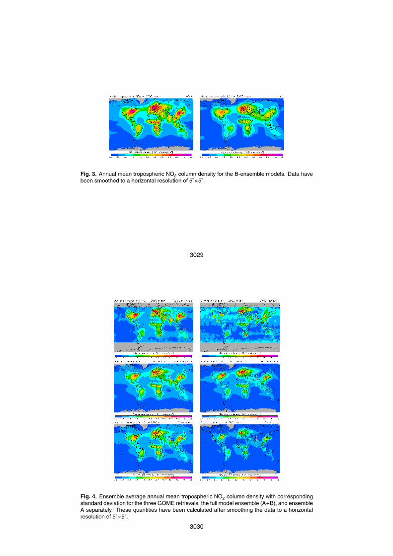
Fig. 3. Annual mean tropospheric NO2 column density for the B-ensemble models. Data havebeen smoothed to a horizontal resolution of 5◦×5◦.

3029

Fig. 4. Ensemble average annual mean tropospheric NO2 column density with correspondingstandard deviation for the three GOME retrievals, the full model ensemble (A+B), and ensembleA separately. These quantities have been calculated after smoothing the data to a horizontalresolution of 5◦×5◦.

3030

Fig. 5. Annual mean tropospheric NO2 column density difference between models and re-trievals for the full model ensemble (A+B) and ensemble A separately. Data have beensmoothed to a horizontal resolution of 5◦×5◦.

3031

Fig. 6. Total sampling bias for ensembles A and B. Data have been smoothed to a horizontalresolution of 5◦×5◦.

3032

Fig. 7. Contribution of day-to-day variability to the sampling bias for ensembles A and B. Herethe B-ensemble mean does not include the MATCH-MPIC and IMAGES models, which providedonly monthly output. Data have been smoothed to a horizontal resolution of 5◦×5◦.

3033

Fig. 8.

3034

Fig. 8. Annual mean tropospheric NO2 column density calculated by application of the averag-ing kernels to the daily 3-dimensional output fields from the three A-ensemble models LMDz-INCA, p-TOMCAT and TM4 (left), together with the difference compared to the correspondingfields shown in Fig. 2, obtained directly from the daily model columns (right). Results for theTM4 model in an alternative setup in which all biomass burning emissions (BBE) are releasedbelow 100 m, are included as well. Data have been smoothed to a horizontal resolution of5◦×5◦.

3035

Fig. 9. Illustration of the various regions analyzed in this study: the east-ern United States (90◦ W–71◦ W×35◦ N–43◦ N), Europe (10◦ W–30◦ E×35◦ N–60◦ N), easternChina (110◦ E–123◦ E×30◦ N–40◦ N), South Africa (26◦ E–31◦ E×28◦ S–23◦ S), Northern Africa(20◦ W–40◦ E×0◦ N–20◦ N), Central Africa (10◦ E–40◦ E×20◦ S–0◦ N), South America (70◦ W–50◦ W×20◦ S–0◦ N), and Southeast Asia (98◦ E–105◦ E×10◦ N–20◦ N).

3036

1 2 3 4 5 6 7 8 9 10 11 12month

0

5

10

15

Tro

posp

heri

c co

lum

n (1

015 m

olec

/cm

2 )

CHASERCTM2FRSGCGEOS-CHEMLMDz-INCAMOZ2-GFDLp-TOMCATTM4TM5

Eastern U.S.

1 2 3 4 5 6 7 8 9 10 11 12month

0

5

10

15

Tro

posp

heri

c co

lum

n (1

015 m

olec

/cm

2 )

LMDz-INCAp-TOMCATTM4BIRA/KNMIBremenDalhousie/SAO

Eastern U.S.

1 2 3 4 5 6 7 8 9 10 11 12month

0

2

4

6

8

Tro

posp

heri

c co

lum

n (1

015 m

olec

/cm

2 )

CHASERCTM2FRSGCGEOS-CHEMLMDz-INCAMOZ2-GFDLp-TOMCATTM4TM5

Europe

1 2 3 4 5 6 7 8 9 10 11 12month

0

2

4

6

8

Tro

posp

heri

c co

lum

n (1

015 m

olec

/cm

2 )

LMDz-INCAp-TOMCATTM4BIRA/KNMIBremenDalhousie/SAO

Europe

Fig. 10.

3037

1 2 3 4 5 6 7 8 9 10 11 12month

0

5

10

15

Tro

posp

heri

c co

lum

n (1

015 m

olec

/cm

2 )

CHASERCTM2FRSGCGEOS-CHEMLMDz-INCAMOZ2-GFDLp-TOMCATTM4TM5

Eastern China

1 2 3 4 5 6 7 8 9 10 11 12month

0

5

10

15

Tro

posp

heri

c co

lum

n (1

015 m

olec

/cm

2 )

LMDz-INCAp-TOMCATTM4BIRA/KNMIBremenDalhousie/SAO

Eastern China

1 2 3 4 5 6 7 8 9 10 11 12month

0

5

10

Tro

posp

heri

c co

lum

n (1

015 m

olec

/cm

2 )

CHASERCTM2FRSGCGEOS-CHEMLMDz-INCAMOZ2-GFDLp-TOMCATTM4TM5

South Africa

1 2 3 4 5 6 7 8 9 10 11 12month

0

5

10

Tro

posp

heri

c co

lum

n (1

015 m

olec

/cm

2 )

LMDz-INCAp-TOMCATTM4BIRA/KNMIBremenDalhousie/SAO

South Africa

Fig. 10.

3038

1 2 3 4 5 6 7 8 9 10 11 12month

0

1

2

3

Tro

posp

heri

c co

lum

n (1

015 m

olec

/cm

2 )

CHASERCTM2FRSGCGEOS-CHEMLMDz-INCAMOZ2-GFDLp-TOMCATTM4TM5

Northern Africa

1 2 3 4 5 6 7 8 9 10 11 12month

0

1

2

3

Tro

posp

heri

c co

lum

n (1

015 m

olec

/cm

2 )

LMDz-INCAp-TOMCATTM4BIRA/KNMIBremenDalhousie/SAO

Northern Africa

1 2 3 4 5 6 7 8 9 10 11 12month

0

1

2

3

4

Tro

posp

heri

c co

lum

n (1

015 m

olec

/cm

2 )

CHASERCTM2FRSGCGEOS-CHEMLMDz-INCAMOZ2-GFDLp-TOMCATTM4TM5

Central Africa

1 2 3 4 5 6 7 8 9 10 11 12month

0

1

2

3

4

Tro

posp

heri

c co

lum

n (1

015 m

olec

/cm

2 )

LMDz-INCAp-TOMCATTM4BIRA/KNMIBremenDalhousie/SAO

Central Africa

Fig. 10.

3039

1 2 3 4 5 6 7 8 9 10 11 12month

0

1

2

3

4

5

Tro

posp

heri

c co

lum

n (1

015 m

olec

/cm

2 )

CHASERCTM2FRSGCGEOS-CHEMLMDz-INCAMOZ2-GFDLp-TOMCATTM4TM5

South America

1 2 3 4 5 6 7 8 9 10 11 12month

0

1

2

3

4

5

Tro

posp

heri

c co

lum

n (1

015 m

olec

/cm

2 )

LMDz-INCAp-TOMCATTM4BIRA/KNMIBremenDalhousie/SAO

South America

1 2 3 4 5 6 7 8 9 10 11 12month

0

1

2

3

4

5

Tro

posp

heri

c co

lum

n (1

015 m

olec

/cm

2 )

CHASERCTM2FRSGCGEOS-CHEMLMDz-INCAMOZ2-GFDLp-TOMCATTM4TM5

Southeast Asia

1 2 3 4 5 6 7 8 9 10 11 12month

0

1

2

3

4

5

Tro

posp

heri

c co

lum

n (1

015 m

olec

/cm

2 )

LMDz-INCAp-TOMCATTM4BIRA/KNMIBremenDalhousie/SAO

Southeast Asia

Fig. 10. Seasonal cycle in the tropospheric NO2 column density for different regions of theworld. Shown are the monthly values obtained from the daily column output from the A-ensemble models (left) or calculated by application of the averaging kernels to the daily 3-dimensional output fields from a subset of models (right), together with the corresponding re-trieval data.

3040

GM

I-C

CM

GM

I-D

AO

GM

I-G

ISS

IMA

GE

SIM

PAC

TM

AT

CH

NC

AR

UL

AQ

CH

ASE

RC

TM

2FR

SGC

GE

OS-

CH

EM

LM

Dz-

INC

AM

OZ

2-G

FDL

p-T

OM

CA

TT

M4

TM

5

BIR

A/K

NM

IB

rem

enD

alh.

/SA

O

0

5

10

15

Tro

posp

heri

c co

lum

n (1

015 m

olec

/cm

2 )

Ensemble BEnsemble AAveraging KernelsRetrievals

Eastern U.S.

GM

I-C

CM

GM

I-D

AO

GM

I-G

ISS

IMA

GE

SIM

PAC

TM

AT

CH

NC

AR

UL

AQ

CH

ASE

RC

TM

2FR

SGC

GE

OS-

CH

EM

LM

Dz-

INC

AM

OZ

2-G

FDL

p-T

OM

CA

TT

M4

TM

5

BIR

A/K

NM

IB

rem

enD

alh.

/SA

O

0

2

4

6

8

Tro

posp

heri

c co

lum

n (1

015 m

olec

/cm

2 )

Ensemble BEnsemble AAveraging KernelsRetrievals

Europe

GM

I-C

CM

GM

I-D

AO

GM

I-G

ISS

IMA

GE

SIM

PAC

TM

AT

CH

NC

AR

UL

AQ

CH

ASE

RC

TM

2FR

SGC

GE

OS-

CH

EM

LM

Dz-

INC

AM

OZ

2-G

FDL

p-T

OM

CA

TT

M4

TM

5

BIR

A/K

NM

IB

rem

enD

alh.

/SA

O0

5

10

15

Tro

posp

heri

c co

lum

n (1

015 m

olec

/cm

2 )

Ensemble BEnsemble AAveraging KernelsRetrievals

Eastern China

GM

I-C

CM

GM

I-D

AO

GM

I-G

ISS

IMA

GE

SIM

PAC

TM

AT

CH

NC

AR

UL

AQ

CH

ASE

RC

TM

2FR

SGC

GE

OS-

CH

EM

LM

Dz-

INC

AM

OZ

2-G

FDL

p-T

OM

CA

TT

M4

TM

5

BIR

A/K

NM

IB

rem

enD

alh.

/SA

O

0

5

10

Tro

posp

heri

c co

lum

n (1

015 m

olec

/cm

2 )

Ensemble BEnsemble AAveraging KernelsRetrievals

South Africa

Fig. 11.

3041

GM

I-C

CM

GM

I-D

AO

GM

I-G

ISS

IMA

GE

SIM

PAC

TM

AT

CH

NC

AR

UL

AQ

CH

ASE

RC

TM

2FR

SGC

GE

OS-

CH

EM

LM

Dz-

INC

AM

OZ

2-G

FDL

p-T

OM

CA

TT

M4

TM

5

BIR

A/K

NM

IB

rem

enD

alh.

/SA

O

0

1

2

3

4

Tro

posp

heri

c co

lum

n (1

015 m

olec

/cm

2 )

Ensemble BEnsemble AAveraging KernelsRetrievals

Northern Africa

GM

I-C

CM

GM

I-D

AO

GM

I-G

ISS

IMA

GE

SIM

PAC

TM

AT

CH

NC

AR

UL

AQ

CH

ASE

RC

TM

2FR

SGC

GE

OS-

CH

EM

LM

Dz-

INC

AM

OZ

2-G

FDL

p-T

OM

CA

TT

M4

TM

5

BIR

A/K

NM

IB

rem

enD

alh.

/SA

O

0

1

2

3

4

Tro

posp

heri

c co

lum

n (1

015 m

olec

/cm

2 )

Ensemble BEnsemble AAveraging KernelsRetrievals

Central Africa

GM

I-C

CM

GM

I-D

AO

GM

I-G

ISS

IMA

GE

SIM

PAC

TM

AT

CH

NC

AR

UL

AQ

CH

ASE

RC

TM

2FR

SGC

GE

OS-

CH

EM

LM

Dz-

INC

AM

OZ

2-G

FDL

p-T

OM

CA

TT

M4

TM

5

BIR

A/K

NM

IB

rem

enD

alh.

/SA

O

0

1

2

3

4

5

Tro

posp

heri

c co

lum

n (1

015 m

olec

/cm

2 )

Ensemble BEnsemble AAveraging KernelsRetrievals

South America

GM

I-C

CM

GM

I-D

AO

GM

I-G

ISS

IMA

GE

SIM

PAC

TM

AT

CH

NC

AR

UL

AQ

CH

ASE

RC

TM

2FR

SGC

GE

OS-

CH

EM

LM

Dz-

INC

AM

OZ

2-G

FDL

p-T

OM

CA

TT

M4

TM

5

BIR

A/K

NM

IB

rem

enD

alh.

/SA

O

0

1

2

3

4

5

Tro

posp

heri

c co

lum

n (1

015 m

olec

/cm

2 )

Ensemble BEnsemble AAveraging KernelsRetrievals

Southeast Asia

Fig. 11. Annual mean tropospheric NO2 column density together with the minimum and max-imum monthly mean values for the different world regions. Results calculated from the dailymodel columns (“Ensemble A”, “Ensemble B”) or the daily 3-dimensional output fields (“Aver-aging Kernels”), are compared to the corresponding retrieval data.

3042

Fig. 12. Annual mean tropospheric NO2 column density calculated with the TM4 model usingGFED emissions for the year 2000 (left), together with the impact of using these emissionsinstead of the average GFED emissions for the years 1997–2002 (see corresponding mapin Fig. 8). Averaging kernels have been applied; data have been smoothed to a horizontalresolution of 5◦×5◦.

3043

Fig. 13. Annual mean tropospheric NO2 column density calculated with the TM4 model usingGFED emissions for the year 2000 and updated emissions factors (EF) (left), together with thechange resulting from using the updated values. Averaging kernels have been applied; datahave been smoothed to a horizontal resolution of 5◦×5◦.

3044

1 2 3 4 5 6 7 8 9 10 11 12month

0

1

2

3

Tro

posp

heri

c co

lum

n (1

015 m

olec

/cm

2 )

TM4TM4/GFED 2000TM4/updated EFBIRA/KNMIBremenDalhousie/SAO

Northern Africa

1 2 3 4 5 6 7 8 9 10 11 12month

0

1

2

3

4

Tro

posp

heri

c co

lum

n (1

015 m

olec

/cm

2 )

TM4TM4/GFED 2000TM4/updated EFBIRA/KNMIBremenDalhousie/SAO

Central Africa

1 2 3 4 5 6 7 8 9 10 11 12month

0

1

2

3

4

5

Tro

posp

heri

c co

lum

n (1

015 m

olec

/cm

2 )

TM4TM4/GFED 2000TM4/updated EFBIRA/KNMIBremenDalhousie/SAO

South America

1 2 3 4 5 6 7 8 9 10 11 12month

0

1

2

3

4

5

Tro

posp

heri

c co

lum

n (1

015 m

olec

/cm

2 )

TM4TM4/GFED 2000TM4/updated EFBIRA/KNMIBremenDalhousie/SAO

Southeast Asia

Fig. 14. Seasonal cycle in the tropospheric NO2 column density for regions dominated bybiomass burning. Shown are the monthly values calculated with the TM4 model using theaverage GFED emissions for the year 1997–2002 or the GFED emissions for the year 2000with and without updated emission factors (EF), together with the corresponding retrieval data.Averaging kernels have been applied to the model data.

3045

1 2 3 4 5 6 7 8 9 10 11 12month

0

2

4

6

8

Tro

posp

heri

c co

lum

n (1

015 m

olec

/cm

2 )

TM4TM4/diurnalBIRA/KNMIBremenDalhousie/SAO

Europe

Fig. 15. Seasonal cycle in the tropospheric NO2 column density for the European region.Shown are the monthly values calculated with the TM4 model with or without diurnal variationsin the anthropogenic NOx emissions in this region, together with the corresponding retrievaldata. Averaging kernels have been applied to the model data.

3046

0 12 24 36 48NO

x lifetime (hours)

0.9

1

1.1

1.2

1.3

Impa

ct a

t 10:

30 lo

cal t

ime

IndustryDomesticTrafficCombined

Diurnal cycle of emissions

Fig. 16. Impact of diurnal variations in emissions on the tropospheric NO2 column at 10:30local time as a function of the lifetime of NOx. Shown are the estimates for the separate anthro-pogenic emission source categories as well as for the combined anthropogenic emissions inthe European region. The dashed black lines indicate the range obtained with the TM4 model.

3047