direct transport of midlatitude stratospheric ozone into ...andreas/publications/92.pdf · direct...

Direct transport of midlatitude stratospheric ozone into the lower

troposphere and marine boundary layer of the tropical Pacific Ocean

O. R. Cooper,1 A. Stohl,1,2 G. Hubler,1 E. Y. Hsie,1 D. D. Parrish,3 A. F. Tuck,3

G. N. Kiladis,3 S. J. Oltmans,4 B. J. Johnson,4 M. Shapiro,5 J. L. Moody,6

and A. S. Lefohn7

Received 18 January 2005; revised 22 June 2005; accepted 1 September 2005; published 13 December 2005.

[1] The detailed survey of midlatitude stratospheric intrusions penetrating into theNorthern Hemisphere tropics was one goal of the Pacific Sub-Tropical Jet Study 2004,conducted from Honolulu, Hawaii, during 19–29 January and 28 February to 15 March.Using the National Oceanic and Atmospheric Administration G-IV jet aircraft,instrumented with dropsondes and a 1-s resolution ozone instrument, we targeted anintrusion above Hawaii on 29 February. The data describe the strongest troposphericozone enhancements ever measured above Hawaii (in comparison to a 22 year ozonesonderecord) and illustrate the mixing of stratospheric ozone into the midtroposphere as aresult of convection triggered by the advection of relatively cold midlatitude air into thetropics. Measurements from the G-IV and Mauna Loa Observatory (3.4 km) showenhanced ozone in the lower troposphere, indicating that the remnants of the intrusionreached these levels. This conclusion is supported by a study using a stratospheric ozonetracer generated by the FLEXPART Lagrangian particle dispersion model. This paper alsodescribes a similar intrusion that enhanced ozone at Mauna Loa on 10 March, as well asHonolulu, which is located in the marine boundary layer. G-IV flights in and out ofHonolulu measured enhanced ozone associated with this event on several occasions. The10 March event transported an estimated 1.75 Tg of ozone into the tropical troposphere,and we suggest that stratospheric intrusions that break away from the polar jet streamas they advect into the tropics are more effective at transporting ozone into the tropospherethan intrusions that remain close to the polar jet stream in midlatitudes. Analysis of thedynamic conditions indicates that the frequency of stratospheric intrusions was notanomalous during January–March 2004. While the 10 March event was by itself anextreme event, strong stratospheric intrusions can be expected to influence the tropicallower troposphere in any year.

Citation: Cooper, O. R., et al. (2005), Direct transport of midlatitude stratospheric ozone into the lower troposphere and marine

boundary layer of the tropical Pacific Ocean, J. Geophys. Res., 110, D23310, doi:10.1029/2005JD005783.

1. Introduction

[2] The chemical composition of the tropical tropospherehas received a great deal of attention over the past 10 to15 years to address issues of air quality on local, regional

and global scales as well as to better understand the Earth’sradiation budget. Ozone is an important trace gas affectingboth photochemical and radiative processes and the impactof anthropogenic and biomass burning emissions on thetropical ozone budget has been well documented [Fishmanet al., 1990; Lelieveld et al., 2001; Thompson et al., 2001,2003; Lelieveld et al., 2004]. During the 1990s, researchersbecame aware that high ozone in the tropics could also havea stratospheric origin. Hubler et al. [1992] examined tracegas measurements from Mauna Loa Observatory (MLO) onthe Island of Hawaii (3.4 km), during spring 1988. Freetropospheric ozone values reached as high as 78 ppbv andmost of the free tropospheric air masses had O3/NOy

correlations consistent with an upper tropospheric/lowerstratospheric origin. During PEM-West A (Northern Hemi-sphere, late summer/early autumn), Browell et al. [1996]used airborne lidar measurements of ozone, water vapor andaerosol backscatter to identify air masses of stratosphericorigin in the troposphere above the tropical North Pacific

JOURNAL OF GEOPHYSICAL RESEARCH, VOL. 110, D23310, doi:10.1029/2005JD005783, 2005

1Cooperative Institute for Research in Environmental Sciences,University of Colorado–NOAA Aeronomy Laboratory, Boulder, Colorado,USA.

2Now at Department of Regional and Global Pollution Issues,Norwegian Institute for Air Research, Kjeller, Norway.

3NOAA Aeronomy Laboratory, Boulder, Colorado, USA.4NOAA Climate Monitoring and Diagnostics Laboratory, Boulder,

Colorado, USA.5NOAA–University Corporation for Atmospheric Research, Boulder,

Colorado, USA.6Department of Environmental Sciences, University of Virginia,

Charlottesville, Virginia, USA.7A.S.L. & Associates, Helena, Montana, USA.

Copyright 2005 by the American Geophysical Union.0148-0227/05/2005JD005783$09.00

D23310 1 of 15

Ocean. They concluded that stratospheric air masses withozone in the 40–60 ppbv range could reach the lowertroposphere down to 1 km and account for 27–40% ofthe lower tropospheric ozone in the central tropical Pacific.They suggested these air masses originated in midlatitudestratospheric intrusions that subsequently descended intothe tropics via the climatological high-pressure system inthe subtropical Pacific. In a related study of the SouthernHemisphere tropics during PEM-Tropics B, Browell et al.[2001] reached similar conclusions. Weller et al. [1996]launched a series of ozonesondes from a ship in the early1990s, reported enhanced ozone in the middle and uppertropical troposphere of the Atlantic, and suggested a possi-ble stratospheric origin, while Tuck et al. [1997] reportedaircraft measurements of several trace gases in the tropicalupper troposphere that indicated a clear midlatitude strato-spheric origin.[3] More recently, surveys of the large aircraft-based data

sets produced by the PEM-West A and B, PEM-Tropics Aand B and Measurement of Ozone and Water Vapor byAirbus In-Service Aircraft (MOZAIC) programs haveshown that layers with trace gas and dynamic traits indic-ative of a stratospheric origin are commonly encounteredthroughout the tropical Pacific free troposphere [Stoller etal., 1999; Thouret et al., 2000, 2001]. Ozonesonde measure-ments from Hong Kong [Liu et al., 2002], Indonesia[Fujiwara et al., 2003] and Hawaii [Oltmans et al., 2004]have also revealed cases of enhanced ozone layers in themiddle and upper troposphere that were linked to a strato-spheric origin. Furthermore, GOME retrievals and a trajec-tory study have associated enhanced tropospheric columnozone above Tahiti in the eastern South Pacific Ocean witha midlatitude stratospheric origin [Ladstatter-Weißenmayeret al., 2004].[4] Current research is also focusing on the actual mech-

anisms that transport ozone from the midlatitude strato-sphere into the tropics. Baray et al. [2000] have shown thatwintertime tropopause folding beneath the subtropical jetstream can lead to downward transport of stratosphericozone into the tropical middle and upper troposphere.Similarly, Rossby wave breaking along the subtropicaltropopause that leads to horizontal stirring of tropical andsubtropical air masses has a maximum frequency in summerover the oceans and downstream of the subtropical high-pressure systems [Postel and Hitchman, 1999], and Scott etal. [2001] have shown that the resulting filamentation ofstratospheric air can transport ozone into the upper tropicaltroposphere. In contrast to these summertime processes,Waugh and Polvani [2000] show that extratropical Rossbywave breaking can cause tongues of air with high potentialvorticity (PV) to penetrate deep into the tropics, with aNorthern Hemisphere maximum occurrence in January.These deep events have been shown to trigger convectionalong the leading edge of the PV tongue [Kiladis, 1998;Waugh and Funatsu, 2003] and to transport ozone into theupper troposphere above Hawaii [Waugh and Funatsu,2003].[5] To date, the most detailed case study of the transport

of stratospheric ozone into the tropics describes a spring-time cutoff low that broke away from the SouthernHemisphere subtropical jet stream and advected into thetropics above Africa as far north as 10�S [Baray et al.,

2003]. The feature persisted for about 2 weeks andslowly decayed. In contrast to a midlatitude cutoff lowthis system became detached from the stratosphere in boththe horizontal and vertical planes. The authors argued thatthe irreversible detachment of the cutoff low from thestratosphere would deposit a significant amount of strato-spheric ozone into the tropical troposphere. However, thisconclusion could not be entirely confirmed as the studywas limited by ozone measurements in the upper tropo-sphere from a single ozonesonde at Reunion Island andtwo MOZAIC flights.[6] Case studies of the mechanisms that transport mid-

latitude stratospheric ozone into the tropics have so far beenlimited to the mid and upper troposphere. While themeasurements from MLO in the late 1980s and the Pacificaircraft-based studies of the 1990s have indicated thatstratospheric air can impact the lower tropical troposphere(LTT), the enhancements were not particularly large and thetransport mechanisms were not explored in detail. To thebest of our knowledge, no study has yet shown thatmidlatitude stratospheric intrusions can have a distinct andstrong impact in the tropical marine boundary layer. Giventhat stratospheric intrusions descend as they head equator-ward approximately along isentropes that extend from themidlatitude stratosphere into the LTT it seems likely thatozone of stratospheric origin should have, on occasion, avery strong impact in the LTT. This hypothesis is supportedby a 15-year climatology of cross tropopause exchange,showing that 4-day trajectories traveling from the midlati-tude stratosphere into the tropical LTT have a maximumwintertime impact along a band stretching from Hawaii toBaja California [James et al., 2003]. It also seems plausiblethat strong intrusions can descend into the marine boundarylayer, perhaps aided by radiational cooling within theintrusion, convection and/or terrain turbulence effects oftropical islands.[7] We hypothesized that wintertime stratospheric intru-

sions should have the potential to strongly impact LTTozone, and that the lack of discussion in the literature on thistopic was due to an absence of measurements that specif-ically target the intrusions as they decay in the tropics. Toaddress this lack of data, the specific targeting of midlati-tude stratospheric intrusions advected into the middle andlower tropical troposphere was one goal of the Pacific Sub-Tropical Jet Study 2004, an initiative of the NationalOceanic and Atmospheric Administration (NOAA) Aeron-omy Laboratory. The study occurred during 19–29 Januaryand 28 February to 15 March and utilized the instrumentedNOAA G-IV aircraft based in Honolulu, Hawaii. The G-IVwas equipped with dropsondes and a 1-s resolution ozoneinstrument. Most of the flights out of Honolulu werededicated to the separate Winter Storms ReconnaissanceProgram 2004 (WSRP), but 3 flights were reserved forexploring stratospheric intrusions. The first flight intercep-ted a stratospheric intrusion just north of Hawaii on29 January. The third flight occurred in March and targetedlow-altitude remnants of a stratospheric intrusion, but airtraffic control prevented the aircraft from flying as low aswas required. This paper describes the second flight, whichoccurred on 29 February and was designed to transect amidlatitude stratospheric intrusion that advected ozone intothe tropics, directly above Hawaii. The data describe the

D23310 COOPER ET AL.: STRATOSPHERIC INTRUSIONS IN THE TROPICS

2 of 15

D23310

strongest tropospheric ozone enhancements ever measuredabove Hawaii (in comparison to a 22 year ozonesonderecord) and illustrate the mixing of stratospheric ozone intothe midtroposphere as a result of convection triggered byrelatively cold midlatitude air advected into the tropics.Measurements from the G-IV and MLO show the ozonereached the LTT. This paper also describes a similarintrusion that enhanced ozone at MLO on 10 March andat Honolulu, which is located in the marine boundary layer.Operational G-IV flights out of Honolulu in support ofWSRP captured enhanced ozone associated with this eventon several occasions.

2. Method

2.1. NOAA G-IV Ozone and Dropsonde Measurements

[8] Ozone was measured on board the NOAA G-IV by aUV absorption instrument based upon the optical benchfrom a commercial instrument (TECO Model 49). Thelamp, mirrors and signal processing electronics werereplaced and the plumbing modified so that the instrumentoperated in a mode similar to that described by Proffitt andMcLaughlin [1983]. One-second ozone measurements weremade with a 1s precision at standard temperature andpressure of approximately 1 ppbv.[9] A series of 12 NCAR GPS dropsondes were released

during the G-IV flight on 29 February. The dropsondeswere designed by the National Center for AtmosphericResearch, Boulder, and constructed by Vaisala Inc.,Woburn, Massachusetts (Vaisala model RD93). Theseinstruments measure temperature, dew point, pressure, andhorizontal and vertical winds, and transmit the data back tothe aircraft twice per second.

2.2. Hilo Ozonesondes

[10] The National Oceanic and Atmospheric Administra-tion’s (NOAA) Climate Monitoring and DiagnosticsLaboratory (CMDL) has launched ozonesondes from Hiloon the Island of Hawaii on a weekly basis since 1982(19.8�N, 155.0�W, 11 m). During special intensive periodsto support field campaigns ozonesondes are launched morefrequently. The balloon-borne ozonesondes were equippedwith the widely used and tested electrochemical concen-tration cell (ECC) sensor [Komhyr, 1969; Komhyr et al.,1995]. ECC sensors have an accuracy of about 10% in thetroposphere, except when ozone is less than 10 ppbv whenaccuracies can be degraded to 15%. Personnel training andinstruments were provided by the Ozone and Water VaporGroup of NOAA CMDL. See Oltmans et al. [1996] for anexplanation of the equipment and techniques employedduring this and many other studies. Prior to April 1998 theozonesondes were prepared with a 1% buffered KI solu-tion. Since April 1998 the ozonesondes were preparedwith a 2% unbuffered KI solution. The different solutionscan result in ozone differences of a few percent but theseerrors are negligible for our goal of simply identifyingtimes when stratospheric ozone intrusions with high ozonemixing ratios were present above Hawaii. For directcomparison to the 1-s G-IV ozone measurements we onlyuse Hilo data since 1991 when a digitized data recorderwas first implemented to allow data collection at a highvertical and temporal resolution. The ozone, temperature

and relative humidity data were partitioned into 100 mvertical layers, and reported as layer averages.

2.3. FLEXPART Stratospheric Ozone Tracer

[11] A stratospheric ozone tracer was calculated by theFLEXPART Lagrangian particle dispersion model [Stohl etal., 1998; Stohl and Thomson, 1999], which simulates thetransport and dispersion of linear tracers by calculatingthe trajectories of a multitude of particles. The model hasbeen applied for case studies of trace gas transport [Stohland Trickl, 1999; Forster et al., 2001; Stohl et al., 2003;Forster et al., 2004] and a climatology of intercontinentaltransport [Stohl et al., 2002; Eckhardt et al., 2003]. Themodel was driven by data from the National Centers forEnvironmental Prediction (NCEP) Global Forecast System(GFS), with a temporal resolution of 3 hours (analyses at0000, 0600, 1200, and 1800 UTC; 3-hour forecasts at 0300,0900, 1500, and 2100 UTC), horizontal resolution of 1� �1�, and 26 vertical levels. Particles are transported both bythe resolved winds and parameterized subgrid motions.FLEXPART parameterizes turbulence in the boundary layerand in the free troposphere by solving Langevin equations[Stohl and Thomson, 1999]. To account for convection,FLEXPART uses the parameterization scheme of Emanueland Zivkovic-Rothman [1999], as described by Seibert et al.[2001].[12] For the analyses in this paper the model was run

from 12 January until 16 March 2004, including severaldays for spin-up time. For this simulation a special featureof FLEXPART was used, which creates a stratospherictracer at the model boundaries that is then advected withinthe model domain [see Stohl et al., 2000]. The domaincovered eastern Asia, the North Pacific basin and NorthAmerica from 1�S to 71�N and 99�E to 61�W. Every modelcolumn on the borders of this domain was split into about100 layers where the mass flux of air was determined atevery time step. For those grid cells along the domainborder that experienced a net flux of air into the domainthe mass of air flowing through these cells was calculated.Once the mass of air entering the model at a grid cellreached a certain threshold (Mair) a trajectory particle (ormore, if required) was positioned at a random location at theboundary of the grid cell. The PV at this position was thendetermined by interpolation from the GFS data. Particleslocated in the troposphere were disregarded (PV < 2potential vorticity units (pvu)). In contrast, stratosphericparticles (PV > 2 pvu) were given a mass according to

MO3¼ Mair � PV � C � 48=29

where C = 60 � 10�9 pvu�1 is the ratio between the ozonevolume mixing ratio and PV in the stratosphere at this timeof the year. The factor 48/29 converts from volume mixingratio to mass mixing ratio. C was taken from Stohl et al.[2000] who found that the average relationship betweenozone and PV in the lowermost stratosphere over Europe asdetermined from ozonesondes was between 58 and 69 ppbv/pvu between January and March.[13] The particles were then allowed to advect through

the stratosphere and into the troposphere according to theGFS winds. Once a particle reached an outflowing bound-ary of the domain it was removed from the simulation. At


3 of 15

D23310

any given time, approximately 40 million particles wereadvected within the model domain. This number fluctuatedslightly, because the mass of air originating in the strato-sphere varies with meteorological situation. Ozone wastreated as a passive tracer and the simulation did not includechemistry or an ozone decay rate, but ozone was depositedat the surface according to a resistance scheme [Wesely,1989]. Ozone fields were output every hour as 1-houraverages at a grid spacing of 0.75� � 0.75�. Grid cellswere 500 m thick between the surface and 14 km, 1000 mthick from 14 to 16 km, and the top layer extended from 16to 20 km. The output ozone fields only provide an estima-tion of the ozone enhancement due to transport from thestratosphere, and any mention of the stratospheric ozonetracer must be thought of as an enhancement to the typicaltropospheric background ozone.[14] The stratospheric ozone tracer was compared to the

1-min average ozone values from all of the G-IV flightsthrough the lower stratosphere during the 2004 WSRPcampaign (above the Pacific, between 15�N and 61�N).The model tended to overestimate ozone when measuredozone was between 100 and 400 ppbv, but underestimatedozone when measured values were greater than 400 ppbv.However, the geometric mean of all the point-by-pointratios of modeled/measured ozone was near unity (0.97),indicating little overall bias in the model. On a point-by-point basis, the standard error of the stratospheric ozonetracer compared to measured ozone was nearly a factor of 2,with much of the error attributed to relatively small errors inthe position or timing of stratospheric features advectedwithin the FLEXPART model. When this comparison islimited to latitudes north of 40�N, where the intrusions inthis paper originated, the model underestimated ozone in thelower stratosphere with a mean modeled/measured ratio of0.9; the standard error of the estimate improved to a factorof 1.5. The flux estimates discussed in Section 4 are forlarge intrusions covering several hundred square kilometersthrough much of the troposphere and originating north of40�N. Therefore the estimated amount of ozone transportedinto the troposphere is expected to be 10% low, with anadditional uncertainty of not more than a factor of 1.5.[15] The FLEXPART stratospheric ozone tracer was also

run in forecast mode during the experiment to assist withflight planning. The model was run four times per dayusing forecast wind fields from the 0000, 0600, 1200 and1800 UTC runs of the NCEP GFS. Forecasts extended120 hours and covered a slightly smaller domain than thatdescribed above and used fewer particles.

2.4. Auxiliary Animations

[16] Two auxiliary animations of the FLEXPART outputare included with this paper.1 While the animations arenot essential for understanding the results presented here,viewing them allows the reader to clearly see the three-dimensional evolution of the midlatitude stratosphericozone intrusions as they are transported into the tropicsand subsequently decay. Animation 1 shows the evolutionof the stratospheric intrusion sampled by the G-IV on29 February 2004, represented by the 100 ppbv isosurface

of the FLEXPART stratospheric ozone tracer. Similarly,Animation 2 shows the tropospheric evolution of theintrusion that impacted Mauna Loa on 10 March 2004(100 ppbv isosurface). The animations can be viewed asanimated GIFs or in QuickTime format with the QuickTimePlayer, freely available at http://www. apple.com/quicktime.

3. Results

3.1. The 29 February Flight

[17] The stratospheric intrusion sampled by the G-IV on29 February 2004 originated several days earlier when alongwave trough formed along the polar jet stream abovethe western North Pacific Ocean on 26 February. By1800 UTC, 27 February, the trough extended well into thetropics and had generated a midlatitude cyclone with itslow-pressure center at 32�N (Figure 1a). A warm conveyorbelt (WCB) formed on the eastern side of the trough andabove the surface low, advecting clouds and moisture to thenortheast; the associated high (cold) cloud tops are clearlyvisible in the GOES-West thermal IR channel (Figure 1a).West of the WCB the cyclone’s dry airstream was advectingtoward the southeast. This feature is evident in Figure 1b asa meridional dry air streamer depicted by the GOES layeraverage specific humidity, a derived product based on theGOES Imager water vapor channel [Moody et al., 1999].The feature is represented in the model fields by the PVcontours on the 300 hPa surface. FLEXPART indicates thatthe stratospheric portion of the dry airstream contained highozone mixing ratios (Figure 1c). The three-dimensionalview of the ozone tracer 100 ppbv isosurface (Figure 1d)shows that the intrusion descended into the middle andlower troposphere (as low as 3.5 km at 21�N) as acontinuous band from the midlatitudes into the tropics. By1800 UTC, 29 February, the storm was isolated from thepolar and subtropical jet streams with a PV anomaly andclosed circulation aloft and a weak surface low located justwest of the upper level low (Figures 1e and 1f). Similar tothe PV anomaly, the FLEXPART ozone tracer shows thatthe ozone advected into the middle and lower tropicaltroposphere had also become detached from its higher-latitude reservoir (Figure 1g). However, the three-dimen-sional view of the ozone 100 ppbv isosurface shows that theintrusion slopes upward from west to east and the uppertropospheric portion is still attached to the stratosphere eastof Hawaii. At this time the intrusion is not as visible in theGOES layer average specific humidity product (Figure 1f)as it has become overrun by relatively moist tropical air[Wimmers and Moody, 2004]. The animation of this intru-sion (Animation 1) illustrates the southward motion of theozone as the storm formed, followed by the intrusion’swest-east elongation over Hawaii where it eventuallydetached from the stratosphere and dispersed.[18] Midlatitude cyclones that extend into the North

Pacific subtropics and tropics during the Northern Hemi-sphere cool season (October-March) are commonly knownas kona storms [Otkin and Martin, 2004]. This particularcyclone fits the definition of a kona storm, and by28 February it had become a classic kona low bringingheavy rainfall to what would normally be the leeward sideof the Hawaiian Islands under typical trade wind conditions.During February 2004 the northwest corner of the Island

1Auxiliary material is available at ftp://ftp.agu.org/apend/jd/2005JD005783.


4 of 15

D23310

Figure 1


5 of 15

D23310

of Hawaii received 200–300% of its normal Februaryprecipitation. Most of the excess precipitation was associ-ated with this particular kona storm, with the rain gauge atKona Village (Station Index 064765) receiving 14.5 cm ofprecipitation during 27–29 February, 97% of the monthlytotal [National Oceanic and Atmospheric Administration,2004].[19] By 1800 UTC, 29 February, the highest cloud tops

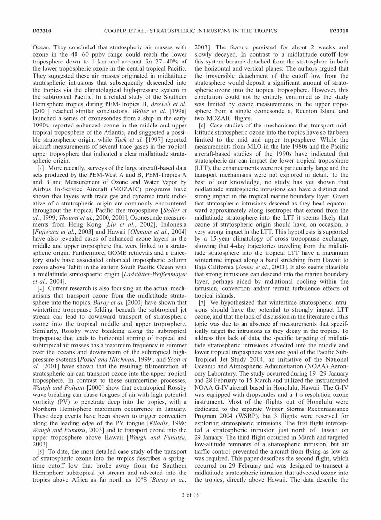
were east of Hawaii, and Figure 1f shows that the highcloud tops are also east of the PV anomaly at the center ofthe kona storm, which is typical of extratropical longwavetroughs that penetrate into the tropics [Kiladis, 1998].Convective clouds and precipitation also occurred beneaththe PV anomaly. Radiosondes from Lihue on the westernside of the Hawaiian Islands showed that the ambienttemperature between 2 and 7 km was 4�–10�C colder whenthe PV anomaly passed over the station in comparison to aquiescent period several days earlier. Similarly, dropsondesreleased from the G-IV into the convective region below thePV anomaly showed temperatures 4�–9�C lower than thereference period at Lihue. As a result of the cold airadvection beneath the PV anomaly, values of convectiveavailable potential energy (CAPE) reached 700 m2 s�2, ascalculated using the methodology of Emanuel [1994].While modest in comparison to severe thunderstorms overthe central United States, a CAPE value of 700 m2 s�2 isconsistent with tropical convection. We conclude that thecold air advected from midlatitudes beneath the PVanomaly destabilized the atmosphere causing convectionand precipitation.[20] Figure 2 shows the flight track that transected the

intrusion, which was planned according to forecasts of theFLEXPART stratospheric ozone tracer. The G-IV took offfrom Honolulu just after 1700 UTC on 29 February andheaded north as it ascended to a cruising altitude of 13 km.During the ascent the G-IV passed through the intrusionbetween 7 and 8 km with ozone reaching 100 ppbv. Uponreaching its cruising altitude the G-IV headed north to26�N, turned and headed south to 16.9�N. During thistransect the aircraft was just below the tropopause andsuccessfully released 12 dropsondes between 25�N and17�N at approximately 80 km intervals (Figure 2c). At thistime the G-IV was above the intrusion and the ozone variedfrom 20 to 50 ppbv. After the dropsondes were released theG-IV flew two north-south transects through the intrusion at8.9 km (ozone up to 280 ppbv) and 6.9 km (ozone up to181 ppbv). To capture some of the east-west structure of theintrusion, the G-IV headedwest at 6.9 km and then performeda short N-S transect at 4.8 km (ozone up to 91 ppbv) during itsreturn to Honolulu.[21] Figure 2 shows elevated ozone along the 8.9 and

6.9 km transects, with enhancements detected from 10.0 km(111 ppbv) down to 3.3 km (72 ppbv). The greater ozonevalues are associated with the very dry air within the intrusion

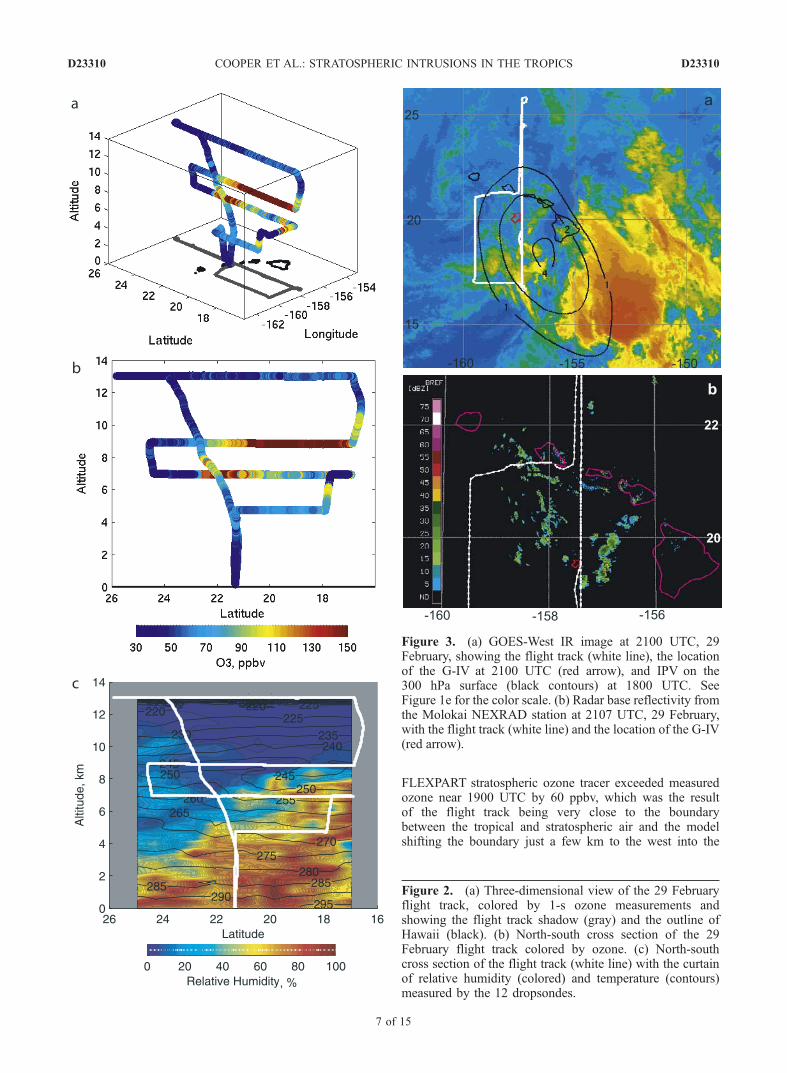
(compare Figures 2a and 2b to Figure 2c). The southernhalf of the transect at 6.9 km has a great deal of ozonevariability, ranging from 31 to 160 ppbv. Because ofconvection this portion of the flight track is much moremoist than the regions of the intrusion sampled at 8.9 kmor along the northern half of the 6.9 km transect. Theconvective cloud tops along this portion of the flight trackare visible in Figure 3a, and the precipitation produced bythe convection is shown in the radar image in Figure 3b.The temperatures of the convective cloud tops near theflight track, as determined by the GOES infrared imageryreached as low as 250 K which corresponds to an altitudeof approximately 7.5 km, as determined from the drop-sondes (Figure 2c) and confirmed by the G-IV flightscientist (coauthor, A. Tuck). Figure 4 shows the 1-sozone measurements versus relative humidity. The dataat 8.9 km were measured above the level of the convectivecloud tops. They show a broad range of ozone but allmeasurements were in very dry air, with relative humidityvalues typically less than 20%, representing the transitionbetween dry tropical midtropospheric air with low ozoneand the dry ozone-rich polar stratospheric air advected intothe tropics. The data at 6.9 km also have a wide range ofozone with greater values generally corresponding to dryair and the lower values generally corresponding to mois-ter air. The range of data points in Figure 4 at this altitudefall along a pseudo mixing line, illustrating the transitionfrom stratospheric air to moist tropical air. (Similar resultswere found when relative humidity was replaced by theconservative quantity of water vapor mixing ratio, allow-ing a true mixing line to be drawn between the dry andmoist air.) Detailed time series for the portion of the flighttrack at 6.9 km (not shown) also indicate that ozone andrelative humidity were anticorrelated with higher humidityand lower ozone values occurring near the convectiveclouds, as observed by the flight scientist. We concludethat the mixing between the stratospheric and troposphericair at 6.9 km was mainly the result of deep convectiveclouds penetrating the base of the intrusion.[22] Figure 5 shows the G-IV ozone time series with the

corresponding FLEXPART stratospheric ozone time seriesinterpolated to the flight track. In these types of comparisonit must be remembered that the stratospheric ozone traceronly estimates the amount of ozone from the stratospherewhile the ozone measurements represent various mixtures ofstratospheric and tropospheric ozone. The ozone tracertracks the measurements fairly well in the sense that highozone corresponds to high tracer values and low ozonecorresponds to low tracer values. There is very goodagreement at 8.9 km between the ozone measurementsand the ozone tracer with maximum ozone reaching260 ppbv and maximum ozone tracer reaching 280 ppbv,indicating that the measured ozone is dominated bystratospheric ozone. The transect at 13 km shows the

Figure 1. (a) GOES-West infrared image with mean sea level pressure, (b) GOES-West layer average specific humidityproduct (purples and blues indicate dry air in the middle to upper troposphere) with 300 hPa IPV contours (contours at 1, 2,4 and 6 pvu) and 250 hPa wind barbs, and (c) FLEXPART stratospheric ozone tracer at 9 km, 1800 UTC, 27 February2004. (d) FLEXPART 100 ppbv ozone isosurface (blue) at 1800 UTC, 27 February, with the terrain of Hawaii (green) andthe 29 February flight track (red) for scale. (e–g) As in Figures 1a–1c but for 1800 UTC, 29 February, with the 29 Februaryflight track superimposed. (h) As in Figure 1d but for 2000 UTC, 29 February; note the different perspective and scale.


6 of 15

D23310

FLEXPART stratospheric ozone tracer exceeded measuredozone near 1900 UTC by 60 ppbv, which was the resultof the flight track being very close to the boundarybetween the tropical and stratospheric air and the modelshifting the boundary just a few km to the west into the

Figure 2. (a) Three-dimensional view of the 29 Februaryflight track, colored by 1-s ozone measurements andshowing the flight track shadow (gray) and the outline ofHawaii (black). (b) North-south cross section of the 29February flight track colored by ozone. (c) North-southcross section of the flight track (white line) with the curtainof relative humidity (colored) and temperature (contours)measured by the 12 dropsondes.

Figure 3. (a) GOES-West IR image at 2100 UTC, 29February, showing the flight track (white line), the locationof the G-IV at 2100 UTC (red arrow), and IPV on the300 hPa surface (black contours) at 1800 UTC. SeeFigure 1e for the color scale. (b) Radar base reflectivity fromthe Molokai NEXRAD station at 2107 UTC, 29 February,with the flight track (white line) and the location of the G-IV(red arrow).


7 of 15

D23310

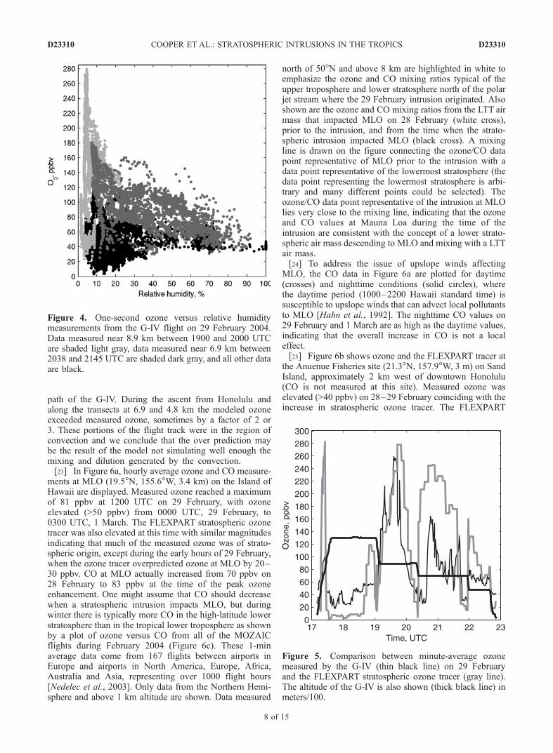
path of the G-IV. During the ascent from Honolulu andalong the transects at 6.9 and 4.8 km the modeled ozoneexceeded measured ozone, sometimes by a factor of 2 or3. These portions of the flight track were in the region ofconvection and we conclude that the over prediction maybe the result of the model not simulating well enough themixing and dilution generated by the convection.[23] In Figure 6a, hourly average ozone and CO measure-

ments at MLO (19.5�N, 155.6�W, 3.4 km) on the Island ofHawaii are displayed. Measured ozone reached a maximumof 81 ppbv at 1200 UTC on 29 February, with ozoneelevated (>50 ppbv) from 0000 UTC, 29 February, to0300 UTC, 1 March. The FLEXPART stratospheric ozonetracer was also elevated at this time with similar magnitudesindicating that much of the measured ozone was of strato-spheric origin, except during the early hours of 29 February,when the ozone tracer overpredicted ozone at MLO by 20–30 ppbv. CO at MLO actually increased from 70 ppbv on28 February to 83 ppbv at the time of the peak ozoneenhancement. One might assume that CO should decreasewhen a stratospheric intrusion impacts MLO, but duringwinter there is typically more CO in the high-latitude lowerstratosphere than in the tropical lower troposphere as shownby a plot of ozone versus CO from all of the MOZAICflights during February 2004 (Figure 6c). These 1-minaverage data come from 167 flights between airports inEurope and airports in North America, Europe, Africa,Australia and Asia, representing over 1000 flight hours[Nedelec et al., 2003]. Only data from the Northern Hemi-sphere and above 1 km altitude are shown. Data measured

north of 50�N and above 8 km are highlighted in white toemphasize the ozone and CO mixing ratios typical of theupper troposphere and lower stratosphere north of the polarjet stream where the 29 February intrusion originated. Alsoshown are the ozone and CO mixing ratios from the LTT airmass that impacted MLO on 28 February (white cross),prior to the intrusion, and from the time when the strato-spheric intrusion impacted MLO (black cross). A mixingline is drawn on the figure connecting the ozone/CO datapoint representative of MLO prior to the intrusion with adata point representative of the lowermost stratosphere (thedata point representing the lowermost stratosphere is arbi-trary and many different points could be selected). Theozone/CO data point representative of the intrusion at MLOlies very close to the mixing line, indicating that the ozoneand CO values at Mauna Loa during the time of theintrusion are consistent with the concept of a lower strato-spheric air mass descending to MLO and mixing with a LTTair mass.[24] To address the issue of upslope winds affecting

MLO, the CO data in Figure 6a are plotted for daytime(crosses) and nighttime conditions (solid circles), wherethe daytime period (1000–2200 Hawaii standard time) issusceptible to upslope winds that can advect local pollutantsto MLO [Hahn et al., 1992]. The nighttime CO values on29 February and 1 March are as high as the daytime values,indicating that the overall increase in CO is not a localeffect.[25] Figure 6b shows ozone and the FLEXPART tracer at

the Anuenue Fisheries site (21.3�N, 157.9�W, 3 m) on SandIsland, approximately 2 km west of downtown Honolulu(CO is not measured at this site). Measured ozone waselevated (>40 ppbv) on 28–29 February coinciding with theincrease in stratospheric ozone tracer. The FLEXPART

Figure 5. Comparison between minute-average ozonemeasured by the G-IV (thin black line) on 29 Februaryand the FLEXPART stratospheric ozone tracer (gray line).The altitude of the G-IV is also shown (thick black line) inmeters/100.

Figure 4. One-second ozone versus relative humiditymeasurements from the G-IV flight on 29 February 2004.Data measured near 8.9 km between 1900 and 2000 UTCare shaded light gray, data measured near 6.9 km between2038 and 2145 UTC are shaded dark gray, and all other dataare black.


8 of 15

D23310

Figure 6. (a) Hourly average ozone (black line), CO (solid circles for nighttime and crosses fordaytime), and FLEXPART stratospheric ozone tracer (gray line) at MLO. (b) Hourly average ozone(black line) and FLEXPART stratospheric ozone tracer at Honolulu. (c) Ozone versus CO from allNorthern Hemisphere MOZAIC flights above 1 km during February 2004. Values measured north of50�N and above 8 km are highlighted (white), and the gray lines indicate the 10th, 50th, and 90th COpercentiles for a given ozone value. Also indicated are the ozone and CO values at MLO for the earlyhours of 28 February (white cross) and the time of the ozone peak at MLO on 29 February (black cross).A mixing line connects the MLO data point (white cross) and an arbitrary point in the lower stratosphere(black diamond).


9 of 15

D23310

stratospheric ozone tracer at the surface was a factor of10 less then the quantity of tracer at 8.9 km along the flighttrack, indicating that the intrusion was diluted by a factor of10 by the time it entered the marine boundary layer.Possible mechanisms for transporting the ozone into themarine boundary layer include convective down drafts[Betts et al., 2002], and turbulent mixing associated withHawaii’s volcanic peaks extending above the marine bound-ary layer. While the enhancements at MLO and Honoluluare not extreme, it appears that this particular extratropicalstratospheric intrusion contributed to the ozone mixingratios in the LTT and tropical marine boundary layer.

3.2. The 10 March Intrusion

[26] The extratropical stratospheric intrusion that impactedMLO on 10March 2004was forecast by FLEXPART but wasnot directly targeted by the G-IVas the aircraft was dedicatedto the separate WSRP experiment at that time. However, theintrusion was intercepted by the G-IVover several days as theaircraft took off and landed in support of WSRP.[27] This intrusion formed in a similar manner to the

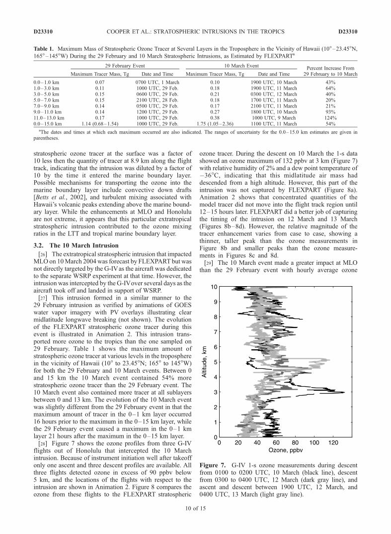
29 February intrusion as verified by animations of GOESwater vapor imagery with PV overlays illustrating clearmidlatitude longwave breaking (not shown). The evolutionof the FLEXPART stratospheric ozone tracer during thisevent is illustrated in Animation 2. This intrusion trans-ported more ozone to the tropics than the one sampled on29 February. Table 1 shows the maximum amount ofstratospheric ozone tracer at various levels in the tropospherein the vicinity of Hawaii (10� to 23.45�N; 165� to 145�W)for both the 29 February and 10 March events. Between 0and 15 km the 10 March event contained 54% morestratospheric ozone tracer than the 29 February event. The10 March event also contained more tracer at all sublayersbetween 0 and 13 km. The evolution of the 10 March eventwas slightly different from the 29 February event in that themaximum amount of tracer in the 0–1 km layer occurred16 hours prior to the maximum in the 0–15 km layer, whilethe 29 February event caused a maximum in the 0–1 kmlayer 21 hours after the maximum in the 0–15 km layer.[28] Figure 7 shows the ozone profiles from three G-IV

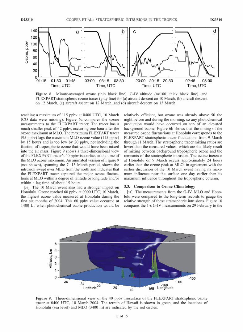
flights out of Honolulu that intercepted the 10 Marchintrusion. Because of instrument initiation well after takeoffonly one ascent and three descent profiles are available. Allthree flights detected ozone in excess of 90 ppbv below5 km, and the locations of the flights with respect to theintrusion are shown in Animation 2. Figure 8 compares theozone from these flights to the FLEXPART stratospheric

ozone tracer. During the descent on 10 March the 1-s datashowed an ozone maximum of 132 ppbv at 3 km (Figure 7)with relative humidity of 2% and a dew point temperature of�36�C, indicating that this midlatitude air mass haddescended from a high altitude. However, this part of theintrusion was not captured by FLEXPART (Figure 8a).Animation 2 shows that concentrated quantities of themodel tracer did not move into the flight track region until12–15 hours later. FLEXPART did a better job of capturingthe timing of the intrusion on 12 March and 13 March(Figures 8b–8d). However, the relative magnitude of thetracer enhancement varies from case to case, showing athinner, taller peak than the ozone measurements inFigure 8b and smaller peaks than the ozone measure-ments in Figures 8c and 8d.[29] The 10 March event made a greater impact at MLO

than the 29 February event with hourly average ozone

Table 1. Maximum Mass of Stratospheric Ozone Tracer at Several Layers in the Troposphere in the Vicinity of Hawaii (10�–23.45�N,165�–145�W) During the 29 February and 10 March Stratospheric Intrusions, as Estimated by FLEXPARTa

29 February Event 10 March Event Percent Increase From29 February to 10 MarchMaximum Tracer Mass, Tg Date and Time Maximum Tracer Mass, Tg Date and Time

0.0–1.0 km 0.07 0700 UTC, 1 March 0.10 1900 UTC, 10 March 43%1.0–3.0 km 0.11 1000 UTC, 29 Feb. 0.18 1900 UTC, 11 March 64%3.0–5.0 km 0.15 0600 UTC, 29 Feb. 0.21 0300 UTC, 12 March 40%5.0–7.0 km 0.15 2100 UTC, 28 Feb. 0.18 1700 UTC, 11 March 20%7.0–9.0 km 0.14 0500 UTC, 29 Feb. 0.17 2100 UTC, 11 March 21%9.0–11.0 km 0.14 1200 UTC, 29 Feb. 0.27 1800 UTC, 10 March 93%11.0–13.0 km 0.17 1000 UTC, 29 Feb. 0.38 1000 UTC, 9 March 124%0.0–15.0 km 1.14 (0.68–1.54) 1000 UTC, 29 Feb. 1.75 (1.05–2.36) 1100 UTC, 11 March 54%

aThe dates and times at which each maximum occurred are also indicated. The ranges of uncertainty for the 0.0–15.0 km estimates are given inparentheses.

Figure 7. G-IV 1-s ozone measurements during descentfrom 0100 to 0200 UTC, 10 March (black line), descentfrom 0300 to 0400 UTC, 12 March (dark gray line), andascent and descent between 1900 UTC, 12 March, and0400 UTC, 13 March (light gray line).


10 of 15

D23310

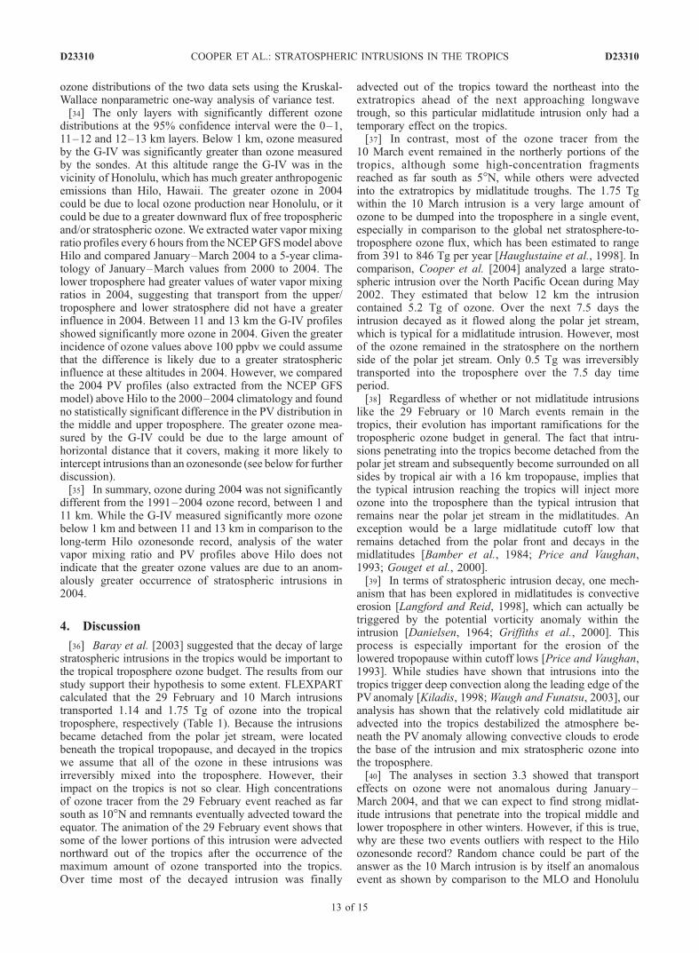
reaching a maximum of 115 ppbv at 0400 UTC, 10 March(CO data were missing). Figure 6a compares the ozonemeasurements to the FLEXPART tracer. The tracer has amuch smaller peak of 42 ppbv, occurring one hour after theozone maximum at MLO. The maximum FLEXPART tracer(95 ppbv) lags the maximum MLO ozone value (115 ppbv)by 15 hours and is too low by 20 ppbv, not including thefraction of tropospheric ozone that would have been mixedinto the air mass. Figure 9 shows a three-dimensional viewof the FLEXPART tracer’s 40 ppbv isosurface at the time ofthe MLO ozone maximum. An animated version of Figure 9(not shown), spanning the 7–13 March period, shows theintrusion swept over MLO from the north and indicates thatthe FLEXPART tracer captured the major ozone fluctua-tions at MLO within a degree of latitude or longitude and/orwithin a lag time of about 15 hours.[30] The 10 March event also had a stronger impact on

Honolulu. Ozone reached 60 ppbv at 0000 UTC, 10 March,the highest ozone value measured at Honolulu during thefirst six months of 2004. This 60 ppbv value occurred at1400 LT when photochemical ozone production would be

relatively efficient, but ozone was already above 50 thenight before and during the morning, so any photochemicalproduction would have occurred on top of an elevatedbackground ozone. Figure 6b shows that the timing of themeasured ozone fluctuations at Honolulu corresponds to theFLEXPART stratospheric tracer fluctuations from 9 Marchthrough 11 March. The stratospheric tracer mixing ratios arelower than the measured values, which are the likely resultof mixing between background tropospheric ozone and theremnants of the stratospheric intrusion. The ozone increaseat Honolulu on 9 March occurs approximately 24 hoursearlier than the ozone peak at MLO, in agreement with theearlier discussion of the 10 March event having its maxi-mum influence near the surface one day earlier than itsmaximum influence throughout the tropospheric column.

3.3. Comparison to Ozone Climatology

[31] The measurements from the G-IV, MLO and Hono-lulu were compared to the long-term records to gauge therelative strength of these stratospheric intrusions. Figure 10compares the 1-s G-IV measurements on 29 February to the

Figure 8. Minute-averaged ozone (thin black line), G-IV altitude (m/100, thick black line), andFLEXPART stratospheric ozone tracer (gray line) for (a) aircraft descent on 10 March, (b) aircraft descenton 12 March, (c) aircraft ascent on 12 March, and (d) aircraft descent on 13 March.

Figure 9. Three-dimensional view of the 40 ppbv isosurface of the FLEXPART stratospheric ozonetracer at 0400 UTC, 10 March 2004. The terrain of Hawaii is shown in green, and the locations ofHonolulu (sea level) and MLO (3400 m) are indicated by the red circles.


11 of 15

D23310

1991–2004 ozonesonde record at Hilo, Hawaii (100 mvertical resolution). The G-IV measurements at 8.9 kmand 6.9 km are greater than the corresponding ozonesondemaximum values by 60 and 80 ppbv, respectively. We alsocompared the 29 February G-IV measurements to the1982–1991 Hilo ozonesonde record (not shown), which islimited by a coarser vertical resolution, and found similarresults. The peak of 72 ppbv at 3.3 km, as well as manyvalues below 2 km, is greater than the Hilo 95th percentile.Similar results were found for the 10 March flight with theozone peak of 132 ppbv at 3 km exceeding the maximumHilo value by more than 40 ppbv (compare Figures 7 and10).[32] Figure 11, created from the full 1973–2004 MLO

ozone record, shows the monthly ozone distribution at MLOillustrating the springtime maximum typical of tropicallocations. The ozone peak of 81 ppbv on 29 February ismuch greater than the February 99th percentile, and theozone peak of 115 ppbv on 10 March equals the previousmaximum value for March. While Honolulu resides in themarine boundary layer its 1994–2003 ozone climatologyalso exhibits a springtime maximum (Figure 12). The ozonepeak of 45 ppbv on 29 February is just below the 99thpercentile, and the ozone peak of 60 ppbv on 10 March isgreater than the previous 1994–2003 March maximum.[33] To determine if 2004 was an anomalous year for

stratospheric intrusions, we compared 22 G-IV ozone pro-files from January–March 2004 to the January–Marchozonesonde record at Hilo for the years 1991–2004 (150

profiles). We excluded all G-IV profiles that specificallytargeted stratospheric intrusions. All G-IV and ozonesondeprofiles were converted to 1 km layer averages. Then foreach kilometer layer between 0 and 13 km we compared the

Figure 10. Comparison between the 1-s G-IV ozone data(gray circles) on 29 February 2004 and the 100-m verticalresolution 1991–2004 ozonesonde climatology at Hilo,Hawaii. Hilo data are summarized as median values (thickline), 25th and 75th percentiles (dashed lines), 5th and 95thpercentiles (thin lines), and minimum and maximum values(medium-weight lines).

Figure 11. MLO hourly average ozone climatology from1973 to 2004 represented as monthly median values (blackline), 25th and 75th percentiles (dashed lines), 1st and 99thpercentiles (gray lines), and minimum and maximum values(circles). The maximum hourly values on 29 February 2004(black cross) and 10 March 2004 (gray cross) are alsoshown.

Figure 12. Honolulu hourly average ozone climatologyfrom 1994 to 2003 represented as monthly median values(black line), 25th and 75th percentiles (dashed lines), 1stand 99th percentiles (gray lines), and minimum andmaximum values (circles). The maximum hourly valueson 29 February 2004 (black cross) and 10 March 2004 (graycross) are also shown.


12 of 15

D23310

ozone distributions of the two data sets using the Kruskal-Wallace nonparametric one-way analysis of variance test.[34] The only layers with significantly different ozone

distributions at the 95% confidence interval were the 0–1,11–12 and 12–13 km layers. Below 1 km, ozone measuredby the G-IV was significantly greater than ozone measuredby the sondes. At this altitude range the G-IV was in thevicinity of Honolulu, which has much greater anthropogenicemissions than Hilo, Hawaii. The greater ozone in 2004could be due to local ozone production near Honolulu, or itcould be due to a greater downward flux of free troposphericand/or stratospheric ozone. We extracted water vapor mixingratio profiles every 6 hours from the NCEPGFSmodel aboveHilo and compared January–March 2004 to a 5-year clima-tology of January–March values from 2000 to 2004. Thelower troposphere had greater values of water vapor mixingratios in 2004, suggesting that transport from the upper/troposphere and lower stratosphere did not have a greaterinfluence in 2004. Between 11 and 13 km the G-IV profilesshowed significantly more ozone in 2004. Given the greaterincidence of ozone values above 100 ppbv we could assumethat the difference is likely due to a greater stratosphericinfluence at these altitudes in 2004. However, we comparedthe 2004 PV profiles (also extracted from the NCEP GFSmodel) above Hilo to the 2000–2004 climatology and foundno statistically significant difference in the PV distribution inthe middle and upper troposphere. The greater ozone mea-sured by the G-IV could be due to the large amount ofhorizontal distance that it covers, making it more likely tointercept intrusions than an ozonesonde (see below for furtherdiscussion).[35] In summary, ozone during 2004 was not significantly

different from the 1991–2004 ozone record, between 1 and11 km. While the G-IV measured significantly more ozonebelow 1 km and between 11 and 13 km in comparison to thelong-term Hilo ozonesonde record, analysis of the watervapor mixing ratio and PV profiles above Hilo does notindicate that the greater ozone values are due to an anom-alously greater occurrence of stratospheric intrusions in2004.

4. Discussion

[36] Baray et al. [2003] suggested that the decay of largestratospheric intrusions in the tropics would be important tothe tropical troposphere ozone budget. The results from ourstudy support their hypothesis to some extent. FLEXPARTcalculated that the 29 February and 10 March intrusionstransported 1.14 and 1.75 Tg of ozone into the tropicaltroposphere, respectively (Table 1). Because the intrusionsbecame detached from the polar jet stream, were locatedbeneath the tropical tropopause, and decayed in the tropicswe assume that all of the ozone in these intrusions wasirreversibly mixed into the troposphere. However, theirimpact on the tropics is not so clear. High concentrationsof ozone tracer from the 29 February event reached as farsouth as 10�N and remnants eventually advected toward theequator. The animation of the 29 February event shows thatsome of the lower portions of this intrusion were advectednorthward out of the tropics after the occurrence of themaximum amount of ozone transported into the tropics.Over time most of the decayed intrusion was finally

advected out of the tropics toward the northeast into theextratropics ahead of the next approaching longwavetrough, so this particular midlatitude intrusion only had atemporary effect on the tropics.[37] In contrast, most of the ozone tracer from the

10 March event remained in the northerly portions of thetropics, although some high-concentration fragmentsreached as far south as 5�N, while others were advectedinto the extratropics by midlatitude troughs. The 1.75 Tgwithin the 10 March intrusion is a very large amount ofozone to be dumped into the troposphere in a single event,especially in comparison to the global net stratosphere-to-troposphere ozone flux, which has been estimated to rangefrom 391 to 846 Tg per year [Hauglustaine et al., 1998]. Incomparison, Cooper et al. [2004] analyzed a large strato-spheric intrusion over the North Pacific Ocean during May2002. They estimated that below 12 km the intrusioncontained 5.2 Tg of ozone. Over the next 7.5 days theintrusion decayed as it flowed along the polar jet stream,which is typical for a midlatitude intrusion. However, mostof the ozone remained in the stratosphere on the northernside of the polar jet stream. Only 0.5 Tg was irreversiblytransported into the troposphere over the 7.5 day timeperiod.[38] Regardless of whether or not midlatitude intrusions

like the 29 February or 10 March events remain in thetropics, their evolution has important ramifications for thetropospheric ozone budget in general. The fact that intru-sions penetrating into the tropics become detached from thepolar jet stream and subsequently become surrounded on allsides by tropical air with a 16 km tropopause, implies thatthe typical intrusion reaching the tropics will inject moreozone into the troposphere than the typical intrusion thatremains near the polar jet stream in the midlatitudes. Anexception would be a large midlatitude cutoff low thatremains detached from the polar front and decays in themidlatitudes [Bamber et al., 1984; Price and Vaughan,1993; Gouget et al., 2000].[39] In terms of stratospheric intrusion decay, one mech-

anism that has been explored in midlatitudes is convectiveerosion [Langford and Reid, 1998], which can actually betriggered by the potential vorticity anomaly within theintrusion [Danielsen, 1964; Griffiths et al., 2000]. Thisprocess is especially important for the erosion of thelowered tropopause within cutoff lows [Price and Vaughan,1993]. While studies have shown that intrusions into thetropics trigger deep convection along the leading edge of thePVanomaly [Kiladis, 1998; Waugh and Funatsu, 2003], ouranalysis has shown that the relatively cold midlatitude airadvected into the tropics destabilized the atmosphere be-neath the PV anomaly allowing convective clouds to erodethe base of the intrusion and mix stratospheric ozone intothe troposphere.[40] The analyses in section 3.3 showed that transport

effects on ozone were not anomalous during January–March 2004, and that we can expect to find strong midlat-itude intrusions that penetrate into the tropical middle andlower troposphere in other winters. However, if this is true,why are these two events outliers with respect to the Hiloozonesonde record? Random chance could be part of theanswer as the 10 March intrusion is by itself an anomalousevent as shown by comparison to the MLO and Honolulu


13 of 15

D23310

ozone records. However, differences in sampling techniquescould also play a role. First, consider the limited samplingof the ozonesondes. For example, between 1991 and 2004there were 648 ozonesonde launches from Hilo. The typicalozonesonde rises at the rate of 5 m/s, which means thesonde spends 200 s in any given 1000 m layer. So the1000 m layer at 8–9 km above Hawaii has been sampledby ozonesondes for a total of 36 hours during the last 13 years,or 0.03% of the time. When this exercise is limited to just theJanuary–March time period, the ozonesondes have onlysampled the 8–9 km layer for approximately 9 hours. Whilethe G-IV did not spend quite as much time in the 8–9 kmlayer, it did specifically target intrusions at this altitude and itsairspeed of 220 m/s allowed it to cover a large horizontaldistance, which ozonesondes cannot accomplish. Second,these intrusions are often associated with severe weatherand ozonesondes are not usually launched in high-wind orhigh-rainfall conditions to avoid damage to the balloon andinstrument payload. Given the limited sampling duration ofthe ozonesondes, their limited horizontal range and theiravoidance of severe weather conditions, perhaps it is notsurprising that the Hilo ozonesondes have not yet measuredozone as great as 280 ppbv at 8–9 km as was seen on the29 February flight that specifically targeted the most intenseregion of a stratospheric intrusion.

5. Conclusions

[41] The new findings from this study are as follows:(1) Lagrangian dispersion models can forecast, with a highdegree of accuracy, the locations of midlatitude stratosphericintrusions as they penetrate into the middle and lowertroposphere of the tropics. (2) Targeted aircraft samplingof such an intrusion revealed the strongest free troposphericozone enhancements ever measured above Hawaii in com-parison to a 22-year ozonesonde record. (3) Cold airadvection associated with the transport of the intrusion intothe tropics produced convective clouds that eroded the baseof the 29 February intrusion, which mixed stratosphericozone into the tropical troposphere. (4) Agreement betweenthe FLEXPART stratospheric ozone tracer and measuredozone fluctuations at Mauna Loa and Honolulu show thatthese intrusions can influence ozone mixing ratios in thelower troposphere and marine boundary layer of the tropics.(5) Transport conditions during winter 2004 were notanomalous, and although the 10 March intrusion was anextreme event, the direct transport of midlatitude strato-spheric ozone into the lower troposphere and marineboundary layer of the tropical Pacific Ocean can beexpected in any winter. (6) We suggest that stratosphericintrusions that break away from the polar jet stream as theyadvect into the tropics are more effective at transportingozone into the troposphere than intrusions that remain closeto the polar jet stream in midlatitudes.[42] In terms of future studies, a full understanding of the

magnitude, structure and lifetime of stratospheric intrusionswithin the tropics and their impact on the tropical andextratropical ozone budget requires targeted aircraft mea-surements. Ideally an aircraft would be dedicated to sam-pling an intrusion on sequential days as it decays in thetropics and descends into the marine boundary layer. Anonboard ozone lidar and measurements of other trace gases

such as CO, NOy and even HCl, which has been shown tobe a good tracer of stratospheric air [Marcy et al., 2004],would help discern the stratospheric contribution to thetropospheric ozone budget. Given the limited flight timeof the G-IV jet aircraft in the lower troposphere, a low-altitude propeller aircraft and/or a lidar instrumented aircraftwould be better suited for tracking intrusions just above andwithin the marine boundary layer.

[43] Acknowledgments. We thank Donna Sueper at the NOAAAeronomy Laboratory for preparing the final aircraft and dropsonde dataand Kenneth Aikin, also at the NOAA Aeronomy Laboratory, for reducingthe final ozone data. Bill Kuster of the NOAA Aeronomy Laboratorymaintained the ozone instrument during the experiment. We also thankP. Novelli at NOAA CMDL for providing the Mauna Loa Observatory COdata, and the Air Surveillance and Analysis Section of the Hawaii StateDepartment of Health for providing the 2004 Honolulu ozone data. Ozoneand CO data measured by in-service Airbus aircraft were provided bythe MOZAIC program. The U.S. Environmental Protection Agency isacknowledged for making the 1994–2003 Honolulu ozone record availableon its Air Quality System database. GOES satellite imagery, NEXRADimagery, and NCEP GFS gridded meteorological fields were provided byUNIDATA Internet delivery and displayed using UNIDATA McIDASsoftware. Finally, we thank the Data Support Section of NCAR’s ScientificComputing Division for making the final run of the 2000–2004 NCEP GFSanalyses available for download.

ReferencesBamber, D. J., P. G.W. Healey, B. M. R. Jones, S. A. Penkett, A. F. Tuck, andG. Vaughan (1984), Vertical profiles of tropospheric gases: Chemical con-sequences of stratospheric intrusions, Atmos. Environ., 18, 1759–1766.

Baray, J.-L., V. Daniel, G. Ancellet, and B. Legras (2000), Planetary-scaletropopause folds in the southern subtropics, Geophys. Res. Lett., 27,353–356.

Baray, J. L., S. Baldy, R. D. Diab, and J. P. Cammas (2003), Dynamicalstudy of a tropical cut-off low over South Africa, and its impact ontropospheric ozone, Atmos. Environ., 37, 1475–1488.

Betts, A. K., L. V. Gatti, A. M. Cordova, M. A. F. Silva Dias, and J. D.Fuentes (2002), Transport of ozone to the surface by convective down-drafts at night, J. Geophys. Res., 107(D20), 8046, doi:10.1029/2000JD000158.

Browell, E. V., et al. (1996), Large-scale air mass characteristics observedover western Pacific Ocean during summertime, J. Geophys. Res., 101,1691–1712.

Browell, E. V., et al. (2001), Large-scale air mass characteristics observedover the remote tropical Pacific Ocean during March–April 1999: Re-sults from PEM-Tropics B field experiment, J. Geophys. Res., 106,32,481–32,501.

Cooper, O. R., et al. (2004), On the life-cycle of a stratospheric intrusionand its dispersion into polluted warm conveyor belts, J. Geophys. Res.,109, D23S09, doi:10.1029/2003JD004006.

Danielsen, E. F. (1964), Report on Project Springfield, DASA 1517, 97 pp.,Def. At. Support Agency, Washington, D. C.

Eckhardt, S., A. Stohl, S. Beirle, N. Spichtinger, P. James, C. Forster,C. Junker, T. Wagner, U. Platt, and S. Jennings (2003), The NorthAtlantic Oscillation controls air pollution transport to the Arctic, Atmos.Chem. Phys., 3, 1769–1778.

Emanuel, K. A. (1994), Atmospheric Convection, Oxford Univ. Press, NewYork.

Emanuel, K. A., and M. Zivkovic-Rothman (1999), Development andevaluation of a convection scheme for use in climate models, J. Atmos.Sci., 56, 1766–1782.

Fishman, J., C. E. Watson, J. C. Larsen, and J. A. Logan (1990), Distribu-tion of tropospheric ozone determined from satellite data, J. Geophys.Res., 95, 3599–3617.

Forster, C., et al. (2001), Transport of boreal forest fire emissions fromCanada to Europe, J. Geophys. Res., 106, 22,887–22,906.

Forster, C., et al. (2004), Lagrangian transport model forecasts and atransport climatology for the Intercontinental Transport and ChemicalTransformation 2002 (ITCT 2K2) measurement campaign, J. Geophys.Res., 109, D07S92, doi:10.1029/2003JD003589.

Fujiwara, M., et al. (2003), Ozonesonde observations in the Indonesianmaritime continent: A case study on ozone rich layer in the equatorialupper troposphere, Atmos. Environ., 37, 353–362.

Gouget, H., G. Vaughan, A. Marenco, and H. G. J. Smit (2000), Decayof a cut-off low and contribution to stratosphere-troposphere exchange,Q. J. R. Meteorol. Soc., 126, 1117–1141.


14 of 15

D23310

Griffiths, M., A. J. Thorpe, and K. A. Browning (2000), Convective desta-bilization by a tropopause fold diagnosed using potential-vorticity inver-sion, Q. J. R. Meteorol. Soc., 126, 125–144.

Hahn, C. J., J. Y. Merrill, and B. G. Mendonca (1992), Meteorologicalinfluences during MLOPEX, J. Geophys. Res., 97, 10,291–10,309.

Hauglustaine, D. A., G. P. Brasseur, S. Walters, P. J. Rasche, J.-F. Muller,L. K. Emmons, and M. A. Carroll (1998), MOZART, a global chemicaltransport model for ozone and related chemical tracers: 2. Model resultsand evaluation, J. Geophys. Res., 103, 28,291–28,335.

Hubler, G., et al. (1992), Total reactive oxidized nitrogen (NOy) in theremote Pacific troposphere and its correlation with O3 and CO: MaunaLoa Observatory Photochemistry Experiment 1988, J. Geophys. Res., 97,10,427–10,447.

James, P., A. Stohl, C. Forster, S. Eckhardt, P. Seibert, and A. Frank (2003),A 15-year climatology of stratosphere-troposphere exchange with aLagrangian particle dispersion model: 2. Mean climate and seasonal varia-bility, J. Geophys. Res., 108(D12), 8522, doi:10.1029/2002JD002639.

Kiladis, G. N. (1998), Observations of Rossby waves linked to convectionover the eastern tropical Pacific, J. Atmos. Sci., 55, 321–339.

Komhyr, W. D. (1969), Electrochemical cells for gas analysis, Ann. Geo-phys., 25, 203–210.

Komhyr, W. D., R. A. Barnes, G. B. Brothers, J. A. Lathrop, and D. P.Opperman (1995), Electrochemical concentration cell ozonesonde perfor-mance evaluation during STOIC 1989, J. Geophys. Res., 100, 9231–9244.

Ladstatter-Weißenmayer, A., J. Meyer-Arnek, A. Schlemm, and J. P.Burrows (2004), Influence of stratospheric airmasses on troposphericvertical O3 columns based on GOME (Global Ozone Monitoring Ex-periment) measurements and backtrajectory calculation over the Paci-fic, Atmos. Chem. Phys., 4, 903–909.

Langford, A. O., and S. J. Reid (1998), Dissipation and mixing of a small-scale stratospheric intrusion in the upper troposphere, J. Geophys. Res.,103, 31,265–31,276.

Lelieveld, J., et al. (2001), The Indian Ocean Experiment: Widespread airpollution from south and Southeast Asia, Science, 291, 1031–1036.

Lelieveld, J., J. van Aardenne, H. Fischer, M. de Reus, J. Williams, andP. Winkler (2004), Increasing ozone over the Atlantic Ocean, Science,302, 1483–1487.

Liu, H., D. J. Jacob, L. Y. Chan, S. J. Oltmans, I. Bey, R. M. Yantosca, J. M.Harris, B. N. Duncan, and R. V. Martin (2002), Sources of troposphericozone along the Asian Pacific Rim: An analysis of ozonesonde observa-tions, J. Geophys. Res., 107(D21), 4573, doi:10.1029/2001JD002005.

Marcy, T. P., et al. (2004), Quantifying stratospheric ozone in the uppertroposphere with in situ measurements of HCl, Science, 304, 261–265.

Moody, J. L., A. J. Wimmers, and J. C. Davenport (1999), Remotely sensedspecific humidity: Development of a derived product from the GOESImager Channel 3, Geophys. Res. Lett., 26, 59–62.

National Oceanic and Atmospheric Administration (2004), Climatologicaldata: Hawaii and Pacific, February 2004, vol. 100, no. 02, http://www5.ncdc.noaa.gov/pubs/publications.html#CD, Natl. Clim. DataCent., Asheville, N. C.

Nedelec, P., J.-P. Cammas, V. Thouret, G. Athier, J.-M. Cousin, C. Legrand,C. Abonnel, F. Lecoeur, G. Cayez, and C. Marizy (2003), An improvedinfrared carbon monoxide analyser for routine measurements aboard com-mercial Airbus aircraft: Technical validation and first scientific results ofthe MOZAIC III programme, Atmos. Chem. Phys., 3, 1551–1564.

Oltmans, S. J., et al. (1996), Summer and spring ozone profiles over theNorth Atlantic from ozonesonde measurements, J. Geophys. Res., 101,29,179–29,200.

Oltmans, S. J., et al. (2004), Tropospheric ozone over the North Pacificfrom ozonesonde observations, J. Geophys. Res., 109, D15S01,doi:10.1029/2003JD003466.

Otkin, J. A., and J. E. Martin (2004), A synoptic climatology of thesubtropical kona storm, Mon. Weather Rev., 132, 1502–1517.

Postel, G. A., and M. H. Hitchman (1999), A climatology of Rossby wavebreaking along the subtropical tropopause, J. Atmos. Sci., 56, 359–373.

Price, J. D., and G. Vaughan (1993), The potential for stratosphere-tropo-sphere exchange in cut-off low systems, Q. J. R. Meteorol. Soc., 119,343–365.

Proffitt, M. H., and R. C. McLaughlin (1983), Fast-response dual-beamUV-absorption ozone photometer suitable for use in stratosphericballoons, Rev. Sci. Instrum., 54, 1719–1728.

Scott, R. K., J.-P. Cammas, and C. Stolle (2001), Stratospheric filamenta-tion into the upper tropical troposphere, J. Geophys. Res., 106, 11,835–11,848.

Seibert, P., B. Kruger, and A. Frank (2001), Parametrisation of convectivemixing in a Lagrangian particle dispersion model, paper presented at

5th GLOREAM Workshop, Paul Scherrer Inst., Wengen, Switzerland,24–26 Sept.

Stohl, A., and D. J. Thomson (1999), A density correction for Lagrangianparticle dispersion models, Boundary Layer Meteorol., 90, 155–167.

Stohl, A., and T. Trickl (1999), A textbook example of long-range transport:Simultaneous observation of ozone maxima of stratospheric and NorthAmerican origin in the free troposphere over Europe, J. Geophys. Res.,104, 30,445–30,462.

Stohl, A., M. Hittenberger, and G. Wotawa (1998), Validation of theLagrangian particle dispersion model FLEXPART against large scaletracer experiment data, Atmos. Environ., 24, 4245–4264.

Stohl, A., N. Spichtinger-Rakowsky, P. Bonasoni, H. Feldmann,M. Memmesheimer, H. E. Scheel, T. Trickl, S. H. Hubener, W. Ringer,and M. Mandl (2000), The influence of stratospheric intrusions onalpine ozone concentrations, Atmos. Environ., 34, 1323–1354.

Stohl, A., S. Eckhardt, C. Forster, P. James, and N. Spichtinger (2002), Onthe pathways and timescales of intercontinental air pollution transport,J. Geophys. Res., 107(D23), 4684, doi:10.1029/2001JD001396.

Stohl, A., C. Forster, S. Eckhardt, N. Spichtinger, H. Huntrieser, J. Heland,H. Schlager, S. Wilhelm, F. Arnold, and O. Cooper (2003), A backwardmodeling study of intercontinental pollution transport using aircraft mea-surements, J. Geophys. Res. , 108(D12), 4370, doi:10.1029/2002JD002862.

Stoller, P., et al. (1999), Measurements of atmospheric layers from theNASA DC-8 and P-3B aircraft during PEM-Tropics A, J. Geophys.Res., 104, 5745–5764.

Thompson, A. M., J. C. Witte, R. D. Hudson, H. Guo, J. R. Herman, andM. Fujiwara (2001), Tropical tropospheric ozone and biomass burning,Science, 291, 2128–2132.

Thompson, A. M., et al. (2003), Southern Hemisphere Additional Ozone-sondes (SHADOZ) 1998–2000 tropical climatology: 2. Troposphericvariability and the zonal wave-one, J. Geophys. Res., 108(D2), 8241,doi:10.1029/2002JD002241.

Thouret, V., J. Y. N. Cho, R. E. Newell, A. Marenco, and H. G. J. Smit(2000), General characteristics of tropospheric trace constituent layersobserved in the MOZAIC program, J. Geophys. Res., 105, 17,379–17,392.

Thouret, V., J. Y. N. Cho, M. J. Evans, R. E. Newell, M. A. Avery, J. D. W.Barrick, G. W. Sachse, and G. L. Gregory (2001), Tropospheric ozonelayers observed during PEM-Tropics B, J. Geophys. Res., 106, 32,527–32,538.

Tuck, A. F., et al. (1997), The Brewer-Dobson circulation in the light ofhigh altitude in situ aircraft observations, Q. J. R. Meteorol. Soc., 123, 1–69.

Waugh, D. W., and B. M. Funatsu (2003), Intrusions into the tropical uppertroposphere: Three-dimensional structure and accompanying ozone andOLR distributions, J. Atmos. Sci., 60, 637–653.

Waugh, D. W., and L. M. Polvani (2000), Climatology of intrusions into thetropical upper troposphere, Geophys. Res. Lett., 27, 3857–3860.

Weller, R., R. Lilischkis, O. Schrems, R. Neuber, and S. Wessel (1996),Vertical ozone distribution in the marine atmosphere over the centralAtlantic Ocean (56�S–50�N), J. Geophys. Res., 101, 1387–1399.

Wesely, M. L. (1989), Parameterization of surface resistances to gaseousdry deposition in regional-scale models, Atmos. Environ., 23, 1293–1304.

Wimmers, A. J., and J. L. Moody (2004), Tropopause folding at satellite-observed spatial gradients: 2. Development of an empirical model,J. Geophys. Res., 109, D19307, doi:10.1029/2003JD004146.

��O. R. Cooper, E. Y. Hsie, G. Hubler, G. N. Kiladis, D. D. Parrish, and

A. F. Tuck, NOAA Aeronomy Laboratory, 325 Broadway, Boulder, CO80305, USA. ([email protected])B. J. Johnson and S. J. Oltmans, NOAA Climate Monitoring and

Diagnostics Laboratory, 325 Broadway, R/GMD1, Boulder, CO 80305-3328, USA.A. S. Lefohn, A.S.L. & Associates, 111 North Last Chance Gulch, Suite

4A, Helena, MT 59601, USA.J. L. Moody, Department of Environmental Sciences, University of

Virginia, Clark Hall, 291 McCormick Road, P. O. Box 400123,Charlottesville, VA 22904-4123, USA.M. Shapiro, NOAA-UCAR, 3450 Mitchell Lane, Boulder, CO 80301,

USA.A. Stohl, Department of Regional and Global Pollution Issues, NILU,

P. O. Box 100, N-2027 Kjeller, Norway.


15 of 15

D23310

direct transport of midlatitude stratospheric ozone into ...andreas/publications/92.pdf · direct...

Documents