tropical tropospheric temperature variations caused …sobel/papers/chiang_sobel.pdf · department...

2616 VOLUME 15J O U R N A L O F C L I M A T E

q 2002 American Meteorological Society

Tropical Tropospheric Temperature Variations Caused by ENSO andTheir Influence on the Remote Tropical Climate*

JOHN C. H. CHIANG

Joint Institute for the Study of the Atmosphere and Ocean, University of Washington, Seattle, Washington, andDepartment of Geography, University of California, Berkeley, Berkeley, California

ADAM H. SOBEL

Department of Applied Physics and Applied Mathematics and Department of Earth and Environmental Sciences,Columbia University, New York, New York

(Manuscript received 20 August 2001, in final form 12 February 2002)

ABSTRACT

The warming of the entire tropical free troposphere in response to El Nino is well established, and suggestsa tropical mechanism for the El Nino–Southern Oscillation (ENSO) teleconnection. The potential impact of thiswarming on remote tropical climates is examined through investigating the adjustment of a single-column modelto imposed tropospheric temperature variations, assuming that ENSO controls interannual tropospheric temper-ature variations at all tropical locations. The column model predicts the impact of these variations in three typicaltropical climate states (precipitation . evaporation; precipitation , evaporation; no convection) over a slabmixed layer ocean. Model precipitation and sea surface temperature (SST) respond significantly to the imposedtropospheric forcing in the first two climate states. Their amplitude and phase are sensitive to the imposed mixedlayer depth, with the nature of the response depending on how fast the ocean adjusts to imposed tropospherictemperature forcing. For larger mixed layer depth, the SST lags the tropospheric temperature by a longer time,allowing greater disequilibrium between atmosphere and ocean. This causes larger surface flux variations, whichdrive larger precipitation variations. Moist convective processes are responsible for communicating the tropo-spheric temperature signal to the surface in this model.

Preliminary observational analysis suggests that the above mechanism may be applicable to interpretinginterannual climate variability in the remote Tropics. In particular, it offers a simple explanation for the grossspatial structure of the observed surface temperature response to ENSO, including the response over land andthe lack thereof over the southeast tropical Atlantic and southeast tropical Indian Oceans. The mechanism predictsthat the air–sea humidity difference variation is a driver of ENSO-related remote tropical surface temperaturevariability, an addition to wind speed and cloudiness variations that previous studies have shown to be important.

1. Introduction

The connection between interannual variations intropical tropospheric temperature (hereafter TT) andENSO is well established (e.g., Horel and Wallace 1981;Pan and Oort 1983; Newell and Wu 1992; Yulaeva andWallace 1994, hereafter YW94; Soden 2000). YW94show in particular that monthly mean 1000–200-mb tro-pospheric temperatures [as measured by the microwavesounding unit (MSU) channel 2 (Spencer and Christy1992)] averaged over the global tropical strip 208S–208N clearly show the warming influence of the 1982/

* Joint Institute for the Study of the Atmosphere and the Ocean/Climate Impact Group Contribution Number 865.

Corresponding author address: J. C. H. Chiang, JISAO, Universityof Washington, Box 354235, Seattle, WA 98195-4235.E-mail: [email protected]

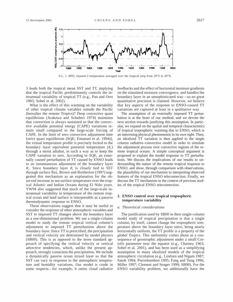
83 and 1986/87 El Nino and the anomalously warmperiod in the first half of the 1990s. The magnitude ofthis warming is around 0.5–18C for strong El Nino years.Figure 1 shows this same analysis updated to December1999, showing in addition the significant response forthe 1997/98 El Nino. This warming occurs almost uni-formly over the global tropical strip (as shown by Fig.4 of YW94).

The reason for this uniform distribution is well un-derstood. The tropical free atmosphere cannot maintainhorizontal pressure gradients, and temperature anoma-lies become uniformly distributed over the global Trop-ics on timescales of a month or two (Charney 1963;Schneider 1977; Held and Hou 1980; Wallace 1992;YW94; Sobel and Bretherton 2000, hereafter SB00).YW94 showed the warming’s close linkage to increasedconvection in the eastern equatorial Pacific. Lag cor-relations between Nino-3 SST, tropical-mean SST, andtropical-mean tropospheric temperature show that Nino-

15 SEPTEMBER 2002 2617C H I A N G A N D S O B E L

FIG. 1. MSU channel-2 temperature averaged over the tropical strip from 208S to 208N.

3 leads both the tropical mean SST and TT, implyingthat the tropical Pacific predominantly controls the in-terannual variability of tropical TT (e.g., Pan and Oort1983; Sobel et al. 2002).

What is the effect of this warming on the variabilityof other tropical climate variables outside the Pacific(hereafter the remote Tropics)? Deep convective quasiequilibrium (Arakawa and Schubert 1974) maintainsthat convection is always sustained so that the convec-tive available potential energy (CAPE) variations re-main small compared to the large-scale forcing ofCAPE. In the limit of zero convective adjustment time[strict quasi equilibrium (SQE; Emanuel et al. 1994)],the virtual temperature profile is precisely locked to theboundary layer equivalent potential temperature (ue)through a moist adiabat, in such a way as to keep theCAPE variation to zero. According to SQE, an exter-nally caused perturbation of TT caused by ENSO leadsto an instantaneous adjustment of the boundary layerue. Since boundary layer ue is closely tied to SSTthrough surface flux, Brown and Bretherton (1997) sug-gested this mechanism as an explanation for the ob-served increase in sea surface temperature over the trop-ical Atlantic and Indian Oceans during El Nino years.YW94 also suggested that much of the large-scale in-terannual variability in temperature of the remote trop-ical ocean and land surface is interpretable as a passivethermodynamic response to ENSO.

These observations suggest that it may be useful toconsider the response of other atmospheric variables andSST to imposed TT changes above the boundary layeras a one-dimensional problem. We use a single-columnmodel to study the remote tropical vertical column’sadjustment to imposed TT perturbations above theboundary layer. Since TT is prescribed, the precipitationand vertical velocity are determined by model physics(SB00). This is as opposed to the more standard ap-proach of specifying the vertical velocity or verticaladvective tendencies, which, unlike the present ap-proach, strongly constrains the precipitation. We includea dynamically passive ocean mixed layer so that theSST can vary in response to the atmospheric tempera-ture and humidity variations. Our model is crude insome respects—for example, it omits cloud radiative

feedbacks and the effect of horizontal moisture gradientson the simulated moisture convergence, and handles theboundary layer in an unsophisticated way—so no greatquantitative precision is claimed. However, we believethat key aspects of the response to ENSO-caused TTvariations are captured at least in a qualitative way.

The assumption of an externally imposed TT pertur-bation is at the heart of our method, and we devote thenext section towards justifying this assumption. In partic-ular, we expand on the spatial and temporal characteristicsof tropical tropospheric warming due to ENSO, which isan interesting physical phenomenon in its own right. Then,an idealized TT variation is then applied to the singlecolumn radiative–convective model in order to simulatethe adjustment process over convective regions of the re-mote tropical oceans. A simple conceptual argument isproposed to explain the model response to TT perturba-tions. We discuss the implications of our results to un-derstanding the nature of the remote tropical response toENSO; and show, through comparison with observations,the plausibility of our mechanism to interpreting observedfeatures of the tropical ENSO teleconnection. Finally, wediscuss the TT mechanism in the context of previous stud-ies of the tropical ENSO teleconnection.

2. ENSO control over tropical tropospherictemperature variability

a. Theoretical considerations

The justification used by SB00 in their single-columnmodel study of tropical precipitation is that a singlecolumn, by itself, cannot change the tropospheric tem-perature above the boundary layer since, being nearlyhorizontally uniform, the TT profile is a property of theglobal Tropics. This uniformity comes about as a con-sequence of geostrophic adjustment under a small Cor-iolis parameter near the equator (e.g., Charney 1963;Sobel et al. 2001), and has been used as a simplifyingassumption in many idealized models of the tropicalatmospheric circulation (e.g., Lindzen and Nigam 1987;Satoh 1994; Pierrehumbert 1995; Fang and Tung 1996;Miller 1997; Clement and Seager 1999; SB00). For theENSO variability problem, we additionally have the


FIG. 2. Lag correlation between the Nino-3 index (SST anomalies averaged between 58S–58N, and1508–908W), and MSU channel-2 temperatures for 1979–99. Light shading is for 0.3 , r , 0.6, anddark is r . 50.6. The number above each panel indicates the lag or lead in months: a 22 implies MSUchannel 2 leads Nino-3 by 2 months.

property that ENSO, as expressed by SST anomalies inthe central and eastern tropical Pacific, controls inter-annual TT variations (YW94; Sobel et al. 2002). Thatthe TT variations can be considered externally imposedin the tropical Atlantic (for example) follows from thefacts that ENSO is generated by coupled ocean–atmo-sphere interactions (in which ocean dynamics play amajor role) in the Pacific (Zebiak and Cane 1987), andthat the tropical Pacific, being a larger basin with stron-ger and more variable deep convection, exerts the dom-inant control on tropical TT variability.

The perturbation vertical TT profile is set by the ver-tical structure of anomalous convection in the ENSOregion. As discussed in Wu et al. (2001), the depth ofconvection in the Pacific source region aids in the rapidtropical redistribution of TT to the rest of the Tropics,since the heating projects onto vertical modes with fasthorizontal propagation speeds.

b. Observational evidenceWe document the transient nature of the MSU chan-

nel-2 TT response to ENSO. A lag correlation between

the ENSO index Nino-3 (defined as the SST anomalyaveraged over 58N–58S, and 1508–908W), and monthlymean 1000–200-mb tropospheric temperatures as mea-sured by MSU channel 2 (Spencer and Christy 1992)is shown in Fig. 2 [see Sobel et al. (2002) for a closelyrelated analysis]. The response can be divided into threephases: growth [25 to 0 months (note that negativemonths are months where MSU leads Nino-3)], mature(11 to 15 months), and decay (16 months and on-ward). In the growth phase, significant warming (r .0.3) occurs in the eastern and central Pacific, exhibitingthe characteristic ‘‘dumbbell shape’’ (YW94) straddlingthe equator. After the establishment of the dumbbellshape, an equatorial warm ‘‘tongue’’ develops and ex-tends westward from the eastern equatorial Pacific. Theequatorial tongue has the appearance of a free Kelvinwave front, though this cannot be confirmed given thecoarse temporal resolution of the dataset used [Bantzerand Wallace (1996) found a similar feature associatedwith the Madden–Julian oscillation using pentad-reso-lution MSU channels 3 and 4, which they interpretedas a Kelvin wave front associated with the switch-on of


an equatorial heat source]. In the mature phase, thewarming extends poleward in both hemispheres. Themaximal extent of the meridional expansion to around308N and S is reached in this phase. Uniformly highcorrelation (r . 0.6) exists throughout the global trop-ical strip except for the western Pacific; the maximumcorrelation averaged over the remote Tropics (608W–908E and 208S–208N) occurs when the MSU field lagsNino-3 by 4 months. The decay phase show the gradualdisappearance of the dumbbell shape in the central andeastern equatorial Pacific and followed by the rest ofthe tropical strip. The signal disappears over the Atlan-tic, Indian, and western Pacific Oceans around 111months.

Pan and Oort (1983) show a similar calculation, butusing upper-air observations from a global radiosondenetwork. Our results generally confirm their findings,although their results do not show the fast propagationof equatorial TT from the eastern equatorial Pacific.

The lag correlation results reinforce the followingpoints: a) the tropical Pacific is the source region forTT variations, b) the signal spreads rapidly throughoutthe entire Tropics, and c) ENSO dominates the inter-annual variability of remote tropical TT. Without ENSO,the variance in monthly mean remote tropical TT anom-alies would be only around half of what is currentlyobserved (Christy and McNider 1994). While our work-ing assumption is that ENSO dominates TT variationsat all tropical locations, the spatial distribution of theabove lag correlation suggests that in reality this as-sumption works best near the equator, and becomes pro-gressively less valid farther away from the equator.

3. Simulations with a single-column model

a. Single-column model

The single-column model is based on the radiative-convective model of Renno et al. (1994). It uses theconvective scheme by Emanuel (1991) and the radiationscheme of Chou et al. (1991). The current model in-cludes vertical advection by the large-scale flow usingan upwind differencing scheme. No explicit vertical dif-fusion is used, although the upwind scheme is implicitlydiffusive. The reader is referred to the original papersfor details of the model parameterizations. The modelvertical resolution is 50 mb from 1000 to 200 mb; 25mb from 200 to 100 mb; and there are nine additionallevels between 100 and 0 mb. The model is set to clear-sky radiation conditions, so that cloud radiative feed-back is not considered. While neglected cloud radiativefeedbacks could potentially be quite important, in deepconvective regimes there is some justification for ne-glecting them in the surface energy budget, since theshortwave and longwave effects of clouds in the Tropicscancel each other to a large degree (e.g., Ramanathanet al. 1989).

Following SB00, we specify the vertical temperature

profile above the planetary boundary layer (PBL; set at825 mb). Horizontal temperature advection is assumednegligible, a good assumption in the deep Tropics; andthe temperature tendency is set to zero above the PBLin accordance with our assumption of imposed TT pro-file. Consequently, the temperature equation becomes abalance between diabatic heating and adiabatic cooling,and hence a diagnostic for the large-scale vertical ve-locity (v). The boundary layer v is found through linearinterpolation (in pressure) from the PBL top v to v 50 at the surface. The moisture equation remains prog-nostic, and includes a moisture convergence that is con-trolled by the vertical velocity diagnosed from the tem-perature equation. Like temperature, horizontal moistureadvection is assumed negligible; its a more questionableassumption but with no easy alternative, since there isno truly correct way to model horizontal advection ex-plicitly in a single-column model. Large-scale verticaladvection of moisture is retained, which implies con-vergence or divergence; effectively, we assume that= · (qv) ù q= ·v. This will tend to exaggerate the mois-ture convergence feedback, since it assumes that whenlocal forcings act to change the local humidity, the hu-midity of adjacent regions (from which moisture is ad-vected) change in lockstep.

A slab ocean mixed layer of prescribed depth is usedfor the surface, so that the model predicts surface tem-perature. While the immediate physical analogy of thissurface parameterization is the surface ocean, it is moregenerally intended as a crude proxy for processes thatdetermine the timescale of the surface temperature re-sponse. In particular, land (small thermal inertia) can becrudely represented by a very shallow mixed layer; andlocations over the surface ocean with strong downgra-dient ocean heat transport can be crudely representedby a very deep mixed layer.

The imposed basic state vertical profile of temperatureis derived from annual average (1979–99) fields fromNational Centers for Environmental Prediction–Nation-al Center for Atmospheric Research (NCEP–NCAR) re-analyses (Kalnay et al. 1996; hereafter, simply the re-analyses) over the global Tropics from 16.258S to16.258N. Radiation is set to annual- and diurnal-averageconditions, and the geographical position at 108N. Thesolar constant is set to 1382 W m22, and CO2 levels to330 ppm. We fix surface wind speed at 6 m s21, whichis close to the annual-mean tropical ocean surface windspeed (between 168N and S) as computed using the DaSilva et al. (1994) dataset.

The perturbation experiments are done for three mod-el mean-state climates: precipitation (P) . evaporation(E), P , E, and no convection. They represent (re-spectively) three distinct regions of the tropical atmo-sphere: a deep convection regime (mean ascent), a shal-low convection regime (mean descent), and a strato-cumulus regime with a stable lower troposphere. Thedifferent mean states are obtained by modifying the al-bedo (see Table 1). This controls the shortwave radiative


TABLE 1. Single-column model parameter settings and equilibri-um results for P . E regime, P , E regime, and no convectionregime.

P . E P , ENo

convection

Lat (8)Mixed layer depth (m)AlbedoPrecipitation (P) (mm day21)Evaporation (E) (mm day21)P 2 E (mm day21)SST (8C)CAPE (J kg21)1000-mb ue (K)

10400.129.675.644.03

28.581330.6

348.6

10400.352.213.61

21.4026.51

392.3344.4

10400.470.691.13

20.4416.94

0315.6

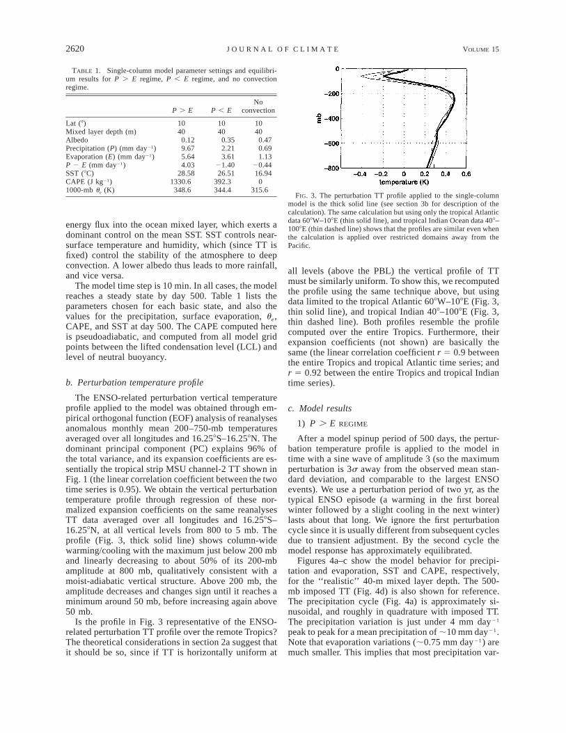
FIG. 3. The perturbation TT profile applied to the single-columnmodel is the thick solid line (see section 3b for description of thecalculation). The same calculation but using only the tropical Atlanticdata 608W–108E (thin solid line), and tropical Indian Ocean data 408–1008E (thin dashed line) shows that the profiles are similar even whenthe calculation is applied over restricted domains away from thePacific.

energy flux into the ocean mixed layer, which exerts adominant control on the mean SST. SST controls near-surface temperature and humidity, which (since TT isfixed) control the stability of the atmosphere to deepconvection. A lower albedo thus leads to more rainfall,and vice versa.

The model time step is 10 min. In all cases, the modelreaches a steady state by day 500. Table 1 lists theparameters chosen for each basic state, and also thevalues for the precipitation, surface evaporation, ue,CAPE, and SST at day 500. The CAPE computed hereis pseudoadiabatic, and computed from all model gridpoints between the lifted condensation level (LCL) andlevel of neutral buoyancy.

b. Perturbation temperature profile

The ENSO-related perturbation vertical temperatureprofile applied to the model was obtained through em-pirical orthogonal function (EOF) analysis of reanalysesanomalous monthly mean 200–750-mb temperaturesaveraged over all longitudes and 16.258S–16.258N. Thedominant principal component (PC) explains 96% ofthe total variance, and its expansion coefficients are es-sentially the tropical strip MSU channel-2 TT shown inFig. 1 (the linear correlation coefficient between the twotime series is 0.95). We obtain the vertical perturbationtemperature profile through regression of these nor-malized expansion coefficients on the same reanalysesTT data averaged over all longitudes and 16.258S–16.258N, at all vertical levels from 800 to 5 mb. Theprofile (Fig. 3, thick solid line) shows column-widewarming/cooling with the maximum just below 200 mband linearly decreasing to about 50% of its 200-mbamplitude at 800 mb, qualitatively consistent with amoist-adiabatic vertical structure. Above 200 mb, theamplitude decreases and changes sign until it reaches aminimum around 50 mb, before increasing again above50 mb.

Is the profile in Fig. 3 representative of the ENSO-related perturbation TT profile over the remote Tropics?The theoretical considerations in section 2a suggest thatit should be so, since if TT is horizontally uniform at

all levels (above the PBL) the vertical profile of TTmust be similarly uniform. To show this, we recomputedthe profile using the same technique above, but usingdata limited to the tropical Atlantic 608W–108E (Fig. 3,thin solid line), and tropical Indian 408–1008E (Fig. 3,thin dashed line). Both profiles resemble the profilecomputed over the entire Tropics. Furthermore, theirexpansion coefficients (not shown) are basically thesame (the linear correlation coefficient r 5 0.9 betweenthe entire Tropics and tropical Atlantic time series; andr 5 0.92 between the entire Tropics and tropical Indiantime series).

c. Model results

1) P . E REGIME

After a model spinup period of 500 days, the pertur-bation temperature profile is applied to the model intime with a sine wave of amplitude 3 (so the maximumperturbation is 3s away from the observed mean stan-dard deviation, and comparable to the largest ENSOevents). We use a perturbation period of two yr, as thetypical ENSO episode (a warming in the first borealwinter followed by a slight cooling in the next winter)lasts about that long. We ignore the first perturbationcycle since it is usually different from subsequent cyclesdue to transient adjustment. By the second cycle themodel response has approximately equilibrated.

Figures 4a–c show the model behavior for precipi-tation and evaporation, SST and CAPE, respectively,for the ‘‘realistic’’ 40-m mixed layer depth. The 500-mb imposed TT (Fig. 4d) is also shown for reference.The precipitation cycle (Fig. 4a) is approximately si-nusoidal, and roughly in quadrature with imposed TT.The precipitation variation is just under 4 mm day21

peak to peak for a mean precipitation of ;10 mm day21.Note that evaporation variations (;0.75 mm day21) aremuch smaller. This implies that most precipitation var-


FIG. 4. P . E model response to imposed TT perturbations, foran MLD of 40 m. (a) Precipitation (solid line) and evaporation (dashedline), (b) SST, (c) CAPE, and (d) imposed 500-mb temperature.

FIG. 5. P . E model response to imposed TT perturbations andvarying MLD. (a) Precipitation, SST, and evaporation peak to peakamplitude as a function of MLD. (b) Phase of the negative precipi-tation anomaly and SST anomaly relative to the imposed TT forcing,as a function of MLD.

iation is due to increased moisture convergence, and notevaporation. As discussed above, the moisture conver-gence effect is likely exaggerated due to the neglect ofhorizontal moisture gradients, since we expect a regionwith mean precipitation of 10 mm day21 to be moisterthan adjacent regions. The SST cycle (Fig. 4b) is alsosinusoidal, and lags imposed TT by about 2 months.The peak to peak amplitude of ;1 K is of the correctmagnitude compared to observed remote tropical SSTvariations with ENSO. The CAPE response (Fig. 4c) isalso sinusoidal, and like precipitation, also approxi-mately in quadrature to imposed TT.

We vary the mixed layer depth (MLD) in the modelto examine the sensitivity of the SST and precipitationresponses to this parameter. The response time series(not shown) are all approximately sinusoidal, but differin amplitude and phase for precipitation and SST. Thephase information is given in months relative to imposedTT. If the imposed TT is

TT 5 A sin(pt/12) (1)

(t is in months), then the phase is computed from

R 5 B sin[p (t 1 w)/12],

212 months , w , 12 months, (2)

where w is chosen so that R has the largest positive

linear correlation to the response. Figure 5 shows theseresponse curves; note, however, that for precipitationwe plot the phase of the negative of the precipitationanomaly, as we usually associate TT warming with re-duced rainfall. The model precipitation and SST re-sponse to MLD is summarized as follows.

• The amplitude of precipitation response increases withincreasing MLD. In particular, for a 1-m MLD theprecipitation peak to peak amplitude is ;1.5 mmday21. The amplitude increases rapidly and approxi-mately linearly to ;8 mm day21 for the 160-m MLD,after which the response tails off. For the fixed SSTcase (infinite MLD), the amplitude is ;8.5 mm day21.

• The amplitude of SST response decreases with in-creasing MLD. The peak to peak amplitude is ;1.2K for the 1-m MLD, and decreases to just less than0.3 K for the 320-m MLD.

• The phase of the negative precipitation anomaly de-creases with increasing MLD; in particular, for the 1-m MLD the phase is around 110 months. The phaserapidly decreases to about 13 months for the 80-mMLD, after which it tails off. For the fixed SST case,the negative precipitation anomaly is almost in phasewith imposed TT.


FIG. 6. Same as in Fig. 4, but for the P , E case. FIG. 7. Same as in Fig. 5, but for the P , E case.

• The SST phase also decreases as MLD increases, thoughthe change is not as pronounced as that for precipitation.SST is almost in phase with TT for the shallow 1-mMLD, and the phase decreases to around 23 monthsfor the 80-m MLD, after which it tails off.

2) P , E REGIME

Figure 6 is the same as Fig. 4 but for the P , Eregime. The variation in SST is similar to that for theP . E case in both amplitude and phase; the same canalso be said for the precipitation phase. The precipitationamplitude (;1 mm day21 peak to peak) is, however,much reduced compared to the P . E case (;4 mmday21). This is not surprising given the smaller meanprecipitation in the P , E case, and that total precipi-tation cannot be negative. Correspondingly, CAPE var-iations are also significantly reduced: ;150 J kg21 ascompared to ;400 J kg21 for the P . E case. Theevaporation peak-to-peak amplitude (;0.5 mm day21)is also reduced compared to the P . E case (;0.75 mmday21), but the reduction is not nearly as much as forprecipitation.

The similarities and differences between P . E andP , E regimes found for the 40-m MLD case hold upif variation with MLD is considered. Figure 7 is thesame as Fig. 5 but for P , E. The phase variation forprecipitation, and both phase and amplitude variations

for SST, with varying MLD is similar to the P . Eregime. The major difference is in the amplitude of pre-cipitation variations, which are reduced by a factor of;6. So, despite the difference in the mean state betweenthe P . E and P , E cases, the model responses arequite similar, except for the amplitude of the precipi-tation (and therefore CAPE) variations.

The model results obtained above appear robust forboth P . E and P , E cases. The amplitude of themodel response is linear with respect to the amplitudeof the TT forcing. We have also repeated the TT per-turbation experiments with quantitatively different P .E and P , E basic states, with similar results.

3) NO-CONVECTION REGIME

We repeat the same 40-m MLD experiment in a re-gime of no model convection. The significant result ofthis experiment (not shown) is that the SST response issignificantly reduced compared to the P . E and P ,E cases. For the 1-m MLD case, the amplitude is reducedby half compared to the P . E and P , E cases; forthe 40-m MLD, the amplitude is reduced by a factor of;6; and for the extreme cases (MLD . 100 m) theamplitude differs by an order of magnitude. With con-vection shut off, updrafts and downdrafts associatedwith convection do not occur, and exchange betweenthe model boundary layer and free troposphere is limited


FIG. 8. The SST adjustment time as a function of MLD, for the P. E (solid line) and P , E (dashed line) regimes. See section 4 forthe derivation.

to large-scale vertical advection and dry adiabatic ad-justment. Our result here implies that it is convectivedowndrafts, in combination with the compensating sub-sidence between clouds that is also included in the con-vection scheme (Emanuel 1991), that is important forcommunicating the free troposphere signal to the surfacein this model. A more sophisticated treatment of thePBL may increase the effectiveness of processes otherthan deep convection in accomplishing this communi-cation, but it is likely that when deep convection isactive it will be the dominant mechanism connectingthe PBL to the free troposphere.

4. Analysis of model results

We argue that the inverse relationship between themodel SST and precipitation amplitude is causallylinked. If the imposed TT is perturbed, then SQE main-tains that subcloud-layer ue (ueb) will follow TT per-turbations over timescales comparable to the convectivetimescale. However this change in ueb will change thethermal disequilibrium between the atmosphere andocean, resulting in a change in surface turbulent energyfluxes (assuming the surface wind speed is fixed, as itis in these simulations). The turbulent fluxes must bal-ance the surface radiative fluxes in steady state. If theradiative fluxes do not change as much as the evapo-ration does in response to the imposed TT change, theresulting imbalance in the surface energy budget willinduce a slow change (compared to the convective time-scale) in the SST, until the SST reaches a value suchthat the turbulent fluxes come back into balance withthe radiative fluxes.

What is the timescale for SST adjustment? In themodel it turns out to be a linear function of the mixedlayer depth (Fig. 8). We computed the adjustment timefor both the P . E and P , E cases by running themodel to equilibrium using the extreme La Nina TTprofile (in other words, the imposed TT profile is themean TT profile subtracted by 3 times the perturbationprofile shown in Fig. 3), and then suddenly switchingto the extreme El Nino (mean TT plus 3 times the Fig.3 perturbation) profile. We took the SST adjustment timeto be the e-folding time for the model SST to adjust tothe new equilibrium state. The point of Fig. 8 is that,for both the P . E and P , E cases, the SST adjustmenttimescale is much faster than the O(1 yr) TT pertur-bation timescale for O(1 m) mixed layer depths, so forthose mixed layer depths the model state is always closeto equilibrium. For realistic ocean mixed layer depths,however, the SST adjustment timescale is an appreciablefraction of the TT perturbation timescale, and so themodel state is continually in adjustment. We hypothesizethat the model response to the ENSO TT forcing de-pends on the ratio of the forcing to SST adjustmenttimescales, and the variation in fluxes and state variablesreflect the state of adjustment of the system to the im-posed TT variations.

We support this hypothesis using another model sen-sitivity run, varying the imposed TT period but keepingthe MLD fixed. Our hypothesis suggests that for fasterTT variations, the ocean mixed layer will be furtherfrom equilibrium, and fluxes between the troposphereand boundary layer (i.e., convection), and between theboundary layer and ocean (i.e., evaporation), will am-plify as a result. On the other hand, variation of statevariables (ueb and SST) will reduce because the systemhas not had sufficient time to respond. In the simulationwe use a 40-m MLD and TT forcing period linearlydecreasing from 3 to 0.5 yr over a 100-model-year in-terval. Figure 9 shows the results for the P . E regime(the P , E result is qualitatively the same). The sim-ulation confirms our hypothesis: both the precipitationand evaporation peak to peak amplitudes increase as theforcing period decreases (Fig. 9a), whereas the SST and1000-mb ue amplitudes decrease with decreasing forcingperiod (Fig. 9b).

We propose this qualitative explanation for the modelsensitivity to the MLD. For a shallow MLD, the SSTquickly adjusts to the TT forcing, and so the SST peakfollows soon after the peak in TT. It follows that surfaceue is able to approximately track the TT forcing andtherefore keep surface flux variations small. This keepsprecipitation variations small as well, because surfaceflux variations control precipitation variations in thisparticular model (SB00). This control can be understoodfrom gross moist stability arguments (Neelin and Held1987; Raymond and Zeng 2000), which say that large-scale vertical motion must be sustained by net input ofmoist static energy through the vertical boundaries ofan atmospheric column, so that anomalously strong con-vection in steady state is driven by anomalously largesurface fluxes (and/or anomalously small radiative cool-ing, a possibility ignored for now). The precipitationphase reflects the phase difference between the TT forc-ing and SST response: basically, the largest imbalancethat causes positive precipitation between the two occurswhen the SST anomaly is still large and the rate ofdecrease of TT is high. Given that both the TT forcing


FIG. 9. The P . E regime response to imposed TT with varying forcing period. The forcing was reducedfrom 3 to 0.5 yr over a 100-yr interval. The curves in (a) and (b) are peak-to-peak amplitudes, computed overa 3-yr time window. (a) Precipitation (solid) and evaporation (dashed) peak-to-peak amplitudes; (b) SST (solid)and 1000-mb ue (dashed) peak-to-peak amplitudes.

and SST response are sinusoidal, this situation occursseveral months after the peak in SST (see Figs. 4 and6). On the other hand, if the MLD is deep, the SSTresponds weakly and the imbalance between TT forcingand SST is large. Surface flux, and therefore precipi-tation, variations are large. Furthermore, because SSTresponds weakly, TT basically controls the phase of theprecipitation variation, such that precipitation is ap-proximately out of phase with TT.

The weakness in all these arguments is the neglectof change in the radiative cooling rate; our argumentholds for the present model because the model lackscloud radiative feedbacks. Therefore, our results con-cerning the magnitude of the precipitation responseshould be regarded as uncertain. We will address thisissue by adding cloud radiative parameterization in fu-ture work. Such a parameterization has already beendeveloped in the context of this model by Bony andEmanuel (2001).

5. Response of the remote Tropics to ENSO

a. Model suggestions

What do the model results suggest with regards tohow TT-mediated ENSO signals manifest themselvesover the global Tropics? The first suggestion is: theresponse, in particular in the precipitation, of the re-mote tropical atmospheric column to TT warming de-pends strongly on the thermal inertia of the surface. Weshow this by forcing the model in the P . E regimewith the amplitude time series associated with the EOF-derived vertical TT perturbation profile (Fig. 3; also seesection 3b). The shape of the EOF time series is almostidentical to the MSU channel-2 Tropics-averaged timeseries shown in Fig. 1, except that the amplitude is 3times larger; we refer to Fig. 1 in lieu of the actual timeseries for future reference. The model SST and precip-itation response at 1-, 40-, and 160-m MLD are shownin Figs. 10a and 10b, respectively. The SST responses

for all three MLD bear resemblance to the forcing TTtime series. Furthermore, the SST response amplitudedecreases for increasing MLD, as expected. On the otherhand, the precipitation response is varied and not readilyassociated with the forcing. In particular, the 1-m MLDresponse is small and differs qualitatively from the 40-and 160-m response. Indicative of this, the associationto ENSO appears to switch sign from the 1-m MLDcase to the 40- and 160-m MLD case: the simultaneouslinear correlation coefficient between the ENSO indexNino-3 and 1-m MLD precipitation time series is r 50.18; on the other hand, the correlation between Nino-3 and the 40-m MLD precipitation time series is r 520.48.

The second suggestion is a ‘‘rule of thumb’’ withregards to the precipitation response. We have argued(section 4) that the further the model is from equilib-rium, the larger the convection and evaporation pertur-bations are. In particular, given a sufficiently large ther-mal inertia of the surface (‘‘sufficient’’ meaning that theSST adjustment timescale is larger than the TT forcingtimescale), the faster TT is changed, the more the oceanand atmosphere will be out of equilibrium, and the larg-er the precipitation response. This is apparent in the40- and 160-m MLD precipitation response in Fig. 10b,when compared to the TT forcing (Fig. 1); in particular,the large dips in the 40-m MLD and 160-m MLD pre-cipitation in late 1982/early 1983 and late 1997/early1998 are associated with steep increases in TT forcing.The dip in precipitation in late 1987/early 1988 is small-er because the TT change was more gradual; this isdespite the fact that the peak TT warming in late 1987/early 1988 is comparable to the 1982/83 event.

Our third suggestion is when and where to expect theSST response. The remote SST will warm by O(1 K)for TT amplitudes used here, but lagged from the peakTT warming by a few months, with the delay increasingas the surface thermal inertia increases. A more signif-icant implication is that while SST will warm in regions


FIG. 10. Results of the single-column model with realistic TT forcing. The imposed TTamplitude is the time series associated with the TT perturbation profile shown in Fig. 3. (a)Model SST time series for the (top) 1-m, (middle) 40-m, and (bottom) 160-m MLD. The tickinterval on the y axis is 0.5 K. (b) Precipitation time series for (top) 1-m, (middle) 40-m, and(bottom) 160-m MLD. The y-axis tick interval is 2 mm day21.

where convection occurs, the SST response will be weakin regions of no significant convection, since the surfacethere is effectively decoupled from the free troposphere(though again we must add a caveat due to the cruderepresentation of the PBL in the present model; strongerentrainment of free tropospheric air into the PBL couldoccur in a more realistic model). The warming occursmainly through a reduction of the latent heat flux, whichis in turn a response to higher surface ue.

b. Comparison to observations

We think our model results are relevant to the ob-served tropical ENSO teleconnection. We will examinethese associations more comprehensively in the future;here, we simply try to convince the reader of the po-tential relevance. Figure 11a shows the linear correlationcoefficient between monthly averaged 40-m MLD-mod-el SST time series of Fig. 10a, and monthly SST anom-alies taken from reanalyses over January 1979 to De-cember 1999. Since the model SST output resemblesthe TT forcing and hence the ENSO signal, it is notsurprising that the correlation map picks out tropicalocean and land regions known from previous studies tobe linked to ENSO. The northern tropical Atlantic, thetropical Indian Ocean, and South China Sea are pre-cisely the locations identified by Klein et al. (1999) as

having significant positive association with eastern Pa-cific SST anomalies. Elliot et al. (2001) previously iden-tified the weaker southwestern tropical Atlantic ENSOsignal. Also in agreement with YW94, we find signif-icant positive correlation with surface temperature (tak-en also from reanalyses January 1979–December 1999)over the tropical land regions 208S–208N (Fig. 11b).The 40-m MLD case is not strictly applicable overland—the 1-m MLD is likely more appropriate—but wenoted before the relative insensitivity of the model sur-face temperature response to MLD. Figure 11a alsoshows that the southeastern (SE) tropical Atlantic andSE tropical Indian Ocean SSTs are not significantly as-sociated with ENSO, in agreement with the Klein et al.(1999).

While the result of the above correlation (Fig. 11) isnot surprising (since the model SST output resemblesthe ENSO forcing), it does point to the viability of ourmodel and the TT mechanism in giving the correct sur-face temperature response. A more powerful result isthat our model offers a simple explanation for the ab-sence of ENSO association in the SE tropical Atlanticand Indian Oceans. Figure 12 shows the annual-meanlow cloud cover from the International Satellite CloudClimatology Project (ISCCP) version D2 dataset (Ros-sow and Schiffer 1991), showing that these regions havelarge low cloud amounts (ISCCP defines low cloud as


FIG. 11. Linear correlation between the 40-m MLD SST time seriesin Fig. 10a and NCEP–NCAR reanalysis surface temperature 1979–99. (top) Over oceans; (bottom) over land. The contour interval is0.15, and magnitudes over 0.3 are shaded. Dashed lines indicatenegative correlation; the zero contour is not shown.

FIG. 12. Annual-mean low cloud cover fraction from ISCCP D2.The contour interval is 0.1, and values above 0.4 are shaded.

clouds with tops below 680 mb). The bulk of the lowclouds in those regions are stratus and stratocumulus.Klein and Hartmann (1993) identified both these regionsas ones possessing significant stratus cloud cover duringall months, implying that they are regions of high staticstability. This implies in turn that the surface is effec-tively decoupled from the free troposphere.

It is possible that the absence of the SST responsemight not be because there is no communication be-tween the free troposphere and PBL, but instead becausethe convective response to TT forcing is counteractedby a stratus cloud response to TT. Stratus cloud coveris positively correlated to vertical static stability (Kleinand Hartmann 1993), implying reduction of net down-ward shortwave surface flux as a result of increasedstratus cloud cover with warmer TT. To test this, weincorporated the effect of stratus cloud change on sur-face fluxes in our model using an empirical methodsimilar to the one used by Philander et al. (1996). Inthis parameterization only the surface flux is affected,and not the model atmospheric radiation budget,amounting to a flux correction for our mixed layerocean. The perturbation in stratus low cloud cover waslinearly related to the anomalous difference in potentialtemperature between 700 mb and the surface based onan observed relationship between the two (Klein andHartmann 1993); and stratus cloud cover perturbationsin turn modified the model downward radiative flux,using an empirical estimate by Norris and Leovy (1994)of 1 W m22 decrease for each 1% increase in cloudcover. We found the impact of this parameterization onour P , E convective case to be small, reducing theSST peak-to-peak amplitude only by ;10% for the 40-m MLD case.

We now focus on precipitation, correlating the month-ly averaged 40-m MLD precipitation time series of Fig.10b with monthly precipitation anomalies from a globalsatellite precipitation dataset spanning January 1979–December 1999 (Xie and Arkin 1997). If the correlationis done over all months, the correlation over the remotetropical regions, with the exception of the Indonesiansubcontinent, is low ( | r | ; 0.1). This is discouragingbut not surprising: precipitation is highly variable on awide range of space- and timescales, and contains muchvariation even on monthly timescales that is (presum-ably) not directly controlled by TT or SST. Additionally,the precipitation signal cannot be large unless there issignificant mean precipitation in the first place. The in-tertropical convergence zone (ITCZ) migrates, so ifthere is an association at any particular location, it islikely to be strong only at specific times of the year. Itimplies we need to take more care with our analysis.

The tropical Atlantic has been identified (e.g., Sara-vanan and Chang 2000; Chiang et al. 2000, 2002; Gi-annini et al. 2001) as a location of significant ENSOinfluence through the anomalous Walker circulation.The tropical Atlantic is the most promising candidatefor our proposed mechanism for several reasons. First,the tropical Atlantic is the colder and smaller of the tworemote tropical ocean basins, implying that any varia-tion in convection there is not likely to feed back sig-nificantly on TT (recall our working assumption that TTvariation is externally controlled by ENSO). Second, itis close to the eastern equatorial Pacific source of anom-alous convective heating, so that the TT signal (cf. Fig.2) reaches the tropical Atlantic with minimal damping.Third, the effective surface thermal inertia in the At-lantic cold tongue region may actually be higher thanwhat a ;50-m or so tropical ocean mixed layer mightsuggest, because equatorial upwelling may act to quick-ly damp surface temperature anomalies; recall that TT-caused precipitation anomalies increase when the sur-face thermal inertia increases. We focus on the January–February–March (JFM) period when the convective per-turbation in the eastern equatorial Pacific is largest(Chiang et al. 2002), but before the tropical AtlanticSST has had time to respond. During those months, theAtlantic ITCZ is also near the equator, within the regionof the strongest ENSO-related TT warming (Fig. 2).


FIG. 13. Linear correlation between the JFM averaged 40-m MLDprecipitation time series in Fig. 10 and Xie–Arkin (1997) global pre-cipitation dataset JFM 1979–99. The contour interval is 0.2, andmagnitudes over 0.4 are shaded. Dashed lines indicate negative cor-relation, and the zero contour is not shown.

Figure 13 shows the JFM correlation between the 40-m MLD precipitation time series of Fig. 10b, and ob-served precipitation over the tropical Pacific and At-lantic. The positive correlation in the Atlantic ITCZregion, and also the neighboring Amazon, are clearlypicked out. The response is not over the equator, butslightly to the north of it, reflecting the mean positionof the ITCZ at that time of year. The rest of the cor-relation map is not as simply explained, and likely dueto ENSO-related causes other than the direct TT warm-ing effect on precipitation. In particular, the negativecorrelation in the north and south subtropical Atlanticmay be associated with the increased baroclinicity thereas a result of jet stream strengthening (YW94).

The direct evidence for TT influence on remote pre-cipitation is not as convincing as that for SST. In par-ticular, the sizable response over the Amazon is sur-prising given that land surfaces are typically thought tohave small thermal inertia. It is possible that adding thecurrently missing physics in our model (see section 6bfor a discussion) may augment the TT signal to producea larger precipitation response over land. A more thor-ough observational analysis is also warranted to takeinto account the seasonality and variability of the remoteprecipitation, and the nature of the remote surface. How-ever, we think there is enough evidence to suggest plau-sibility of the TT mechanism to significantly affect re-mote precipitation variability.

c. The TT mechanism in the context of previoustropical ENSO teleconnection studies

Previous observational studies of the remote tropicalresponse to ENSO [e.g., Curtis and Hastenrath 1995;Klein et al. 1999 (and references therein); Yu and Ri-enecker 1999] focused on the causes of SST change inthe remote tropical oceans. In general, these studies con-cluded that changes in latent heat flux due to surfacewind speed changes and/or solar radiation due to change

in cloud cover generate remote SST anomalies. Surfaceheat flux change due to change in surface temperatureand specific humidity (hereafter T–q changes) has thusfar not been shown to play a role. However, currenthistorical records of observational surface flux are tooinaccurate for budget studies; consequently, while windspeed and cloud cover can be shown (as in the above-cited studies) to be correlated with SST change, we areaware of no budget analysis that shows quantitativelythat these influences are much larger than the mecha-nism discussed here involving T–q. Furthermore, latentheat flux change caused by boundary layer T–q changeis difficult to detect observationally for two reasons: (i)boundary layer T–q are highly correlated to surface SSTat monthly timescales because of fast turbulent and con-vective processes linking the surface to the PBL (e.g.,Betts and Ridgeway 1989), making cause and effectdifficult to assess; and (ii) the fact that the surface fluxesrespond strongly to T–q perturbations will keep thoseperturbations small even if their effect on the fluxes islarge. A typical 10 W m22 anomaly in latent heat fluxrequires a surface–air humidity difference anomaly ofaround 0.4 g kg21 (estimated from the bulk formula withstandard coefficients and 6 m s21 wind speed), whichis the same magnitude as an estimated mean randomerror of 1.1 g kg21 for the marine 10-m specific humiditymeasurements from voluntary observing ships (Kent etal. 1999).

However, flux budget calculations can be done withgeneral circulation model (GCM) studies. In this regard,the recent comprehensive atmospheric GCM study bySaravanan and Chang (2000, p. 2186) lends support fora significant role for T–q: ‘‘Our analysis . . . show[s]that changes in the wind speed and changes in the air-sea temperature difference can both contribute to theheat flux anomalies. This conclusion is somewhat dif-ferent from other studies of surface heat flux variabilityin the Tropics, which tend to focus only on the effectof wind speed changes on the latent and sensible heatflux.’’ The atmospheric GCM–mixed layer ocean ENSOteleconnection study by Lau and Nath (2001) also showsthat surface air temperature changes lead SST in thenorthwestern tropical Atlantic (site E of Fig. 7e in theirpaper), suggesting a significant role for T–q, althoughthose authors do not report the strength of this effectrelative to wind speed and cloudiness change.

In lieu of direct observational evidence, we appeal tothe combination of potential explanatory power andsimplicity offered by the mechanism proposed here. Us-ing straightforward physical reasoning (weak horizontalTT gradients, convective quasi equilibrium) in a one-dimensional context, it can explain the gross large-scalespatial features of the ENSO-related surface temperatureresponse over both tropical oceans and land (note thatthe observational studies mentioned above do not ad-dress mechanisms for the land response). Cloud-coverfeedbacks can actually be straightforwardly includedunder our approach once we include a parameterization


of these effects in the model. Wind speed changes, onthe other hand, are location specific and not derivablefrom a one-dimensional argument. Because of this, it isnot simple to show detailed spatial correlation betweenwind speed change and SST change.

The causes of surface temperature response to ENSOover the remote tropical regions remain an open ques-tion to be decided ultimately by more accurate surfaceflux measurements. It is likely that wind speed and cloudcover are significant components of this variability. Wepropose additionally, based on our model results and inagreement with Saravanan and Chang (2000), that theT–q effect is also important. The relative importance ofeach mechanism may depend on region: the TT mech-anism will have the strongest effect near the equatorwhere the ENSO-caused TT signal is strongest and thepresence of convection most effectively mediates thesignal to the surface. The wind speed mechanism maywork best in the trade wind region (this is certainly thecase for SST variability for the north tropical Atlantic).We are uncertain where cloud effects will be strongest,though the study by Klein et al. suggests that they aremost effective in the regions of deep convection.

6. Summary and discussion

a. Summary

Interannual tropical tropospheric temperature (TT)variations are dominated by ENSO. We study its po-tential impact on the remote Tropics by imposing TTvariations on a single-column model coupled to a slabocean mixed layer, and investigating its response. Thisapproach is based on assumptions that ENSO-causedTT anomalies are horizontally uniform, and there is nosignificant feedback on TT by the remote tropical re-sponse. We examine the model response to the variationsunder P . E, P , E, and no-convection mean condi-tions, and test model sensitivity to varying ocean mixedlayer depth.

Experiments on the 40-m MLD single-column modelusing a 2-yr period sine wave TT perturbation showedthat the model precipitation and surface temperature re-sponse resembles the forcing but with significant phaseshift. In particular, the SST maximum occurs 2 monthsfollowing the peak TT. The size of the response to TTforcing (forcing magnitude comparable to the largestENSO events) is significant in climate terms: SST re-sponse is O(1 K), and precipitation amplitude is a sig-nificant fraction of the total mean precipitation. Withvarying MLD, the phase and amplitude of both the SSTand precipitation responses change markedly: the SSTamplitude decreases and phase shift increases with in-creasing MLD; and the precipitation amplitude increasesand phase shift also increases with increasing MLD. Ina regime with no significant convection, the model SSTresponse is an order of magnitude smaller than the casesover convective regimes. The implication is that com-

munication between the free troposphere and boundarylayer/surface in this model is brought about predomi-nantly by moist convection.

We hypothesize that the timescale of SST adjustmentrelative to the TT forcing timescale controls the modelsensitivity to MLD. A larger heat storage capacity forthe ocean implies that SST takes longer to come toequilibrium with the imposed TT forcing. The more theSST and boundary layer are out of equilibrium with thefree troposphere, the larger the fluxes between them(meaning convection and evaporation). A simulation inwhich we change the period of the TT forcing, keepingMLD fixed, confirms this hypothesis.

Our results lead to these suggestions with regards tofinding TT-related ENSO signals in the remote Tropics:(a) the amplitude and phase of the SST and precipitationresponse depend on the surface thermal inertia; (b) thefaster the rate of TT change (;anomalous convectionin the central and eastern equatorial Pacific), the largerthe remote precipitation response; and (c) the TT signalpropagates to the surface only in regions of (deep orshallow) convection.

We show evidence that the TT mechanism is appli-cable to observed SST and precipitation variability inthe Tropics outside the ENSO region. Given observedTT forcing for 1979–99, the model produces SST var-iations resembling those over tropical ocean regionsknown to be linked to ENSO. The model January–Feb-ruary–March (JFM) averaged precipitation response iscorrelated to JFM precipitation anomalies in the tropicalAtlantic, in agreement with previous studies that arguefor a linkage between ENSO and precipitation there viathe anomalous Walker circulation. Furthermore, the TTmechanism offers a simple explanation for the lack ofSST response over the tropical SE Atlantic and tropicalSE Indian Oceans: that the stable lower troposphere (asevidenced by the stratus cloud decks) precludes the sur-face and boundary layer from being linked to the freetroposphere by convection.

Previous observational studies of the ENSO telecon-nection have shown that variations in cloud cover andwind speed are significant drivers of the ENSO-relatedremote tropical SST variability. No observational evi-dence has yet been shown for a role for air–sea tem-perature and humidity difference changes as predictedby the TT mechanism. However, observed marine fluxesare known to have significant uncertainties; and recentGCM studies have shown a role for temperature andhumidity difference to drive SST variability. In lieu ofdirect observational evidence, we appeal to the com-bination of potential explanatory power and simplicityoffered by the TT mechanism to argue its relevance inremote tropical climate variability.

b. Discussion

There are several potentially important processes thatwe have purposefully simplified or neglected in our


study, and we summarize them here. ENSO-relatedcloud variations may alter the TT-forced responsethrough changing the surface and top-of-atmosphere ra-diative balance. There is some cancellation of surfaceradiative flux changes due to change in deep convectionfrom the shortwave and longwave components (e.g.,Ramanathan et al. 1989); however, this may not be thecase in shallow convective and stratus deck regions. Inparticular, stratus cloud variations may amplify throughpositive feedback on SST (e.g., Philander et al. 1996).We intend to repeat these experiments in the future,using a more realistic single-column model that includescloud–radiation feedback.

Neglect of horizontal moisture advection may exag-gerate the precipitation variations in our model. Whilequantitatively likely to be significant, in general it isdifficult to see how it can change the qualitative senseof the convective adjustment to imposed TT variations,unless the regions adjacent to our column (from whichmoisture is advected) undergo large and covaryingmoisture change. We have also neglected the feedbackon convection through modifying the large-scale (sur-face) horizontal flow. Convection is thought to drivelarge-scale circulation in the Tropics (e.g., Gill 1980),and which in turn potentially feeds back on itself inseveral ways: (a) through surface evaporation (‘‘wind-evaporation feedback’’; Neelin et al. 1987); (b) throughSST via ocean dynamical processes (upwelling; mixedlayer depth change; Ekman or geostrophic transports;or thermocline displacement); and (c) through changesin horizontal moisture advection.

We have shown that the surface is important to howthe atmosphere responds to TT perturbations. Clearly,the ocean is not just a slab mixed layer as is assumedin this study. Variations in mixed layer depth changesthe thermal inertia of the ocean surface, sometimes dras-tically, on seasonal and interannual timescales. Oceanheat transport (OHT) processes may damp surface flux–generated SST anomalies. The damping effect of theseOHT processes may mean that the effective mixed layerdepth is deeper than the typical ;40 m we assumed astypical for the tropical oceans. As for land, the twoimportant differences that matter to the TT mechanismare the smaller thermal inertia of land relative to theocean, and the reduction in evaporation due to waterstress. We have already shown the sensitivity of themodel response to surface thermal inertia (section 5).Water stress over land means that cooling of the surfaceby evaporation is far less than over the ocean, and thesurface temperature response will be larger. Feedbackprocesses may also come into play: less convectionmeans a drier surface, and hence less evaporation andtherefore convection. On the other hand, a drier surfaceis also a warmer surface, and monsoon flows driven bythe surface temperature contrasts may act against thepositive land-evaporation feedback. A realistic land pa-rameterization is thus crucial to study the effects of

ENSO-related TT perturbations over remote tropicalland regions.

Our method is predicated on the assumption that theresponse in the remote Tropics does not feed back ontothe TT. How good is this assumption? A remote precip-itation response to the ENSO-caused TT signal indicatesdiabatic heating changes, and hence feedback on TT. Forthe tropical Atlantic precipitation response, we think thedamping is small because the Atlantic El Nino (Zebiak1993)—which accounts for much of the non-ENSO in-terannual variability of the Atlantic ITCZ—does not ex-plain significant amounts of the tropical TT variance,implying the same for the ENSO-linked variations. Onthe other hand, Bantzer and Wallace (1996) show thatvariations in convection largely concentrated in the In-dian Ocean region do significantly affect Tropicswide TTon the intraseasonal timescale, suggesting that IndianOcean convection has the potential to feed back moreeffectively on ENSO-caused TT variations. The issue offeedback will be addressed in the future.

We end by discussing the interpretation of our mech-anism. Much of the ‘‘atmospheric bridge’’ (Lau andNath 1996) thinking of tropical ENSO teleconnectionsis in terms of the Walker circulation and its impact onremote tropical climate through suppression of rainfallby subsidence (e.g., Kumar et al. 1999; Goddard andGraham 1999; Chiang et al. 2000). The TT mechanismis (more or less) this Walker mechanism, just posed ina different way (our method can be viewed as the lim-iting case of a two-box model for zonal interactions ofthe tropical climate where one box is much larger thanthe other; it is remarkable that nature has provided uswith an example of this). The problem with the tradi-tional way of thinking is that it does not allow for morethan just the qualitative statement that ‘‘rainfall is sup-pressed.’’ This is because the Walker circulation is es-sentially a (horizontal) dynamical construct (e.g., Gill1980) while the problem actually requires understandingthe thermodynamics. When more precise questions areasked, for example—Where does the subsidence occur?How much rainfall is suppressed, and when? What isthe difference in the response between ocean and landregions? What about the difference between deep con-vection/shallow convection/no convection regions?—the value of our approach becomes self-evident.

Acknowledgments. We thank Yochanan Kushnir forhis advice and encouragement throughout this project,and Kerry Emanuel for providing the single-columnmodel and for his prompt response to our many ques-tions. We also thank Richard Seager, Mike Wallace,Chris Bretherton, Clara Deser, R. Saravanan, David Bat-tisti, and Michela Biasutti for helpful conversations.JCHC is supported through the NOAA Postdoctoral Pro-gram in Climate and Global Change, administered bythe University Corporation for Atmospheric Research;and by the Joint Institute for the Study of the Atmo-sphere and Ocean/Climate Impact Group (JISAO/CIG)


under NOAA Cooperative Agreement NAI17RJ1232.AHS is supported through NSF Grant ATM-0096195,NASA grant NAG5-10607, and a Fellowship for Sci-ence and Engineering from the David and Lucile Pack-ard Foundation.

REFERENCES

Arakawa, A., and W. H. Schubert, 1974: Interaction of a cumuluscloud ensemble with the large-scale environment. Part I. J. At-mos. Sci., 31, 674–701.

Bantzer, C. H., and J. M. Wallace, 1996: Intraseasonal variability intropical mean temperature and precipitation and their relation tothe tropical 40–50 day oscillation. J. Atmos. Sci., 53, 3032–3045.

Betts, A. K., and W. Ridgeway, 1989: Climatic equilibrium of theatmospheric convective boundary layer over a tropical ocean. J.Atmos. Sci., 46, 2621–2641.

Bony, S., and K. A. Emanuel, 2001: A parameterization of the cloud-iness associated with cumulus convection: Evaluation usingTOGA COARE data. J. Atmos. Sci., 58, 3158–3183.

Brown, R. G., and C. S. Bretherton, 1997: A test of the strict quasi-equilibrium theory on long time and space scales. J. Atmos. Sci.,54, 624–638.

Charney, J. G., 1963: A note on large-scale motions in the tropics.J. Atmos. Sci., 20, 607–609.

Chiang, J. C. H., Y. Kushnir, and S. E. Zebiak, 2000: Interdecadalchanges in eastern Pacific ITCZ variability and its influence onthe Atlantic ITCZ. Geophys. Res. Lett., 27, 3687–3690.

——, ——, and A. Giannini, 2002: Deconstructing Atlantic ITCZvariability: Influence of the local cross-equatorial SST gradient,and remote forcing from the eastern equatorial Pacific. J. Geo-phys. Res., 107, (D1), 148–227.

Chou, M.-D., D. P. Krantz, and W. Ridgeway, 1991: Infrared heatingparameterizations in numerical climate models. J. Climate, 4,424–437.

Christy, J. R., and R. T. McNider, 1994: Satellite greenhouse signal.Nature, 367, 325.

Clement, A., and R. Seager, 1999: Climate and the tropical oceans.J. Climate, 12, 3383–3401.

Curtis, S., and S. Hastenrath, 1995: Forcing of anomalous sea-surfacetemperature evolution in the tropical Atlantic during Pacificwarm events. J. Geophys. Res., 100, 15 835–15 847.

Da Silva, A. M., C. C. Young, and S. Levitus, 1994: Algorithms andProcedures. Vol. 1, Atlas of Surface Marine Data 1994, U. S.Department of Commerce, National Oceanic and AtmosphericAdministration, 83 pp.

Elliot, J. R., S. P. Jewson, and R. T. Sutton, 2001: The impact of the1997/98 El Nino event of the Atlantic Ocean. J. Climate, 14,1069–1077.

Emanuel, K. A., 1991: A scheme for representing cumulus convectionin large-scale models. J. Atmos. Sci., 48, 2313–2335.

——, J. D. Neelin, and C. S. Bretherton, 1994: On large-scale cir-culation in convecting atmospheres. Quart. J. Roy. Meteor. Soc.,120, 1111–1143.

Fang, M., and K. K. Tung, 1996: A simple model of nonlinear Hadleycirculation with an ITCZ: Analytic and numerical solutions. J.Atmos. Sci., 53, 1241–1261.

Giannini, A., J. C. H. Chiang, M. A. Cane, Y. Kushnir, and R. Seager,2001: The ENSO teleconnection to the tropical Atlantic Ocean:Contributions of the remote and local SSTs to rainfall variabilityin the tropical Americas. J. Climate, 14, 4530–4544.

Gill, A. E., 1980: Some simple solutions for the heat-induced tropicalcirculation. Quart. J. Roy. Meteor. Soc., 106, 447–462.

Goddard, L., and N. E. Graham, 1999: Importance of the Indian Oceanfor simulating rainfall anomalies over eastern and southern Af-rica. J. Geophys. Res., 104 (D16), 19 099–19 116.

Held, I. M., and A. Y. Hou, 1980: Nonlinear axially symmetric cir-culations in a nearly inviscid atmosphere. J. Atmos. Sci., 37,515–533.

Horel, J. D., and J. M. Wallace, 1981: Planetary-scale atmosphericphenomena associated with the Southern Oscillation. Mon. Wea.Rev., 109, 813–829.

Kalnay, E., and Coauthors, 1996: The NCEP/NCAR 40-Year Re-analysis Project. Bull. Amer. Meteor. Soc., 77, 437–471.

Kent, E. C., P. G. Challenor, and P. K. Taylor, 1999: A statisticaldetermination of the random observational errors present in vol-untary observing ships’ meteorological reports. J. Atmos. Oce-anic Technol., 16, 905–914.

Klein, S. A., and D. L. Hartmann, 1993: The seasonal cycle of lowstratiform clouds. J. Climate, 6, 1587–1606.

——, B. J. Soden, and N.-C. Lau, 1999: Remote sea surface tem-perature variations during ENSO: Evidence for a tropical at-mospheric bridge. J. Climate, 12, 917–932.

Kumar, K. K., B. Rajagopalan, and M. A. Cane, 1999: On the weak-ening relationship between the Indian monsoon and ENSO. Sci-ence, 284, 2156–2159.

Lau, N.-C., and M. J. Nath, 1996: The role of the atmospheric bridgein linking tropical Pacific ENSO events to extratropical SSTanomalies. J. Climate, 9, 2036–2057.

——, and ——, 2001: Impact of ENSO on SST variability in theNorth Pacific and North Atlantic: Seasonal dependence and roleof extratropical sea–air coupling. J. Climate, 14, 2846–2866.

Lindzen, R. S., and S. Nigam, 1987: On the role of sea-surface tem-perature gradients in forcing low-level winds and convergencein the tropics. J. Atmos. Sci., 44, 2418–2436.

Miller, R. L., 1997: Tropical thermostats and low cloud cover. J.Climate, 10, 409–440.

Neelin, J. D., and I. M. Held, 1987: Modeling tropical convergencebased on the moist static energy budget. Mon. Wea. Rev., 115,3–12.

——, ——, and K. H. Cook, 1987: Evaporation-wind feedback andlow-frequency variability in the tropical atmosphere. J. Atmos.Sci., 44, 2341–2348.

Newell, R. E., and Z.-X. Wu, 1992: The interrelationships betweentemperature changes in the free atmosphere and sea surface tem-perature changes. J. Geophys. Res., 97 (D4), 3693–3709.

Norris, J. R., and C. B. Leovy, 1994: Interannual variability in strat-iform cloudiness and sea surface temperature. J. Climate, 7,1915–1925.

Pan, Y. H., and A. H. Oort, 1983: Global climate variations connectedwith sea surface temperature anomalies in the eastern equatorialPacific Ocean for the 1958–73 period. Mon. Wea. Rev., 111,1244–1258.

Philander, S. G. H., D. Gu, G. Lambert, N.-C. Lau, T. Li, and R. C.Pacanowski, 1996: Why the ITCZ is mostly north of the equator.J. Climate, 9, 2958–2972.

Pierrehumbert, R. T., 1995: Thermostats, radiator fins, and the localrunaway greenhouse. J. Atmos. Sci., 52, 1784–1806.

Ramanathan, V., R. D. Cess, E. F. Harrison, P. Minnis, B. R. Bark-strom, E. Ahmad, and D. Hartmann, 1989: Cloud-radiative forc-ing and climate: Results from the Earth Radiation Budget Ex-periment. Science, 243, 57–63.

Raymond, D. J., and X. Zeng, 2000: Instability and large-scale cir-culations in a two-column model of the tropical troposphere.Quart. J. Roy. Meteor. Soc., 126, 3117–3135.

Renno, N. O., K. A. Emanuel, and P. H. Stone, 1994: Radiative–convective model with an explicit hydrologic cycle. 1: Formu-lation and sensitivity to model parameters. J. Geophys. Res., 99,14 429–14 441.

Rossow, W. B., and R. A. Schiffer, 1991: International satellite cloudclimatology project (ISCCP) cloud data products. Bull. Amer.Meteor. Soc., 72, 2–20.

Saravanan, R., and P. Chang, 2000: Interaction between tropical At-lantic variability and El Nino–Southern Oscillation. J. Climate,13, 2177–2194.

Satoh, M., 1994: Hadley circulation in radiative–convective equilib-rium in an axially symmetric atmosphere. J. Atmos. Sci., 51,1947–1968.

Schneider, E. K., 1977: Axially symmetric steady-state models of the


basic state for instability and climate studies. Part II: Nonlinearcalculations. J. Atmos. Sci., 34, 280–296.

Sobel, A. H., and C. S. Bretherton, 2000: Modeling tropical precip-itation in a single column. J. Climate, 13, 4378–4392.

——, J. Nilsson, and L. M. Polvani, 2001: The weak temperaturegradient and balanced tropical moisture waves. J. Atmos. Sci.,58, 3650–3665.

——, I. M. Held, and C. S. Bretherton, 2002: The ENSO signal intropical tropospheric temperature. J. Climate, 15, 2702–2706.

Soden, B. J., 2000: The sensitivity of the tropical hydrological cycleto ENSO. J. Climate, 13, 538–549.

Spencer, R. W., and J. R. Christy, 1992: Precision and radiosondevalidation of satellite gridpoint temperature anomalies. Part I:MSU channel 2. J. Climate, 5, 847–857.

Wallace, J. M., 1992: Effect of deep convection on the regulation oftropical sea-surface temperatures. Nature, 357, 230–231.

Wu, Z., E. S. Sarachik, and D. S. Battisti, 2001: Thermally driventropical circulations under Rayleigh friction and Newtonian cool-ing: Analytic solutions. J. Atmos. Sci., 58, 724–741.

Xie, P., and P. A. Arkin, 1997: Global Precipitation: A 17-year month-ly analysis based on gauge observations, satellite estimates, andnumerical model outputs. Bull. Amer. Meteor. Soc., 78, 2539–2558.

Yu, L., and M. M. Rienecker, 1999: Mechanisms for the Indian Oceanwarming during the 1997–98 El Nino. Geophys. Res. Lett., 26,735–738.

Yulaeva, E., and J. M. Wallace, 1994: The signature of ENSO inglobal temperature and precipitation fields derived from the mi-crowave sounding unit. J. Climate, 7, 1719–1736.

Zebiak, S. E., 1993: Air–sea interaction in the equatorial Atlanticregion. J. Climate, 6, 1567–1568.

——, and M. A. Cane, 1987: A model El Nino–Southern Oscillation.Mon. Wea. Rev., 115, 2262–2278.

tropical tropospheric temperature variations caused …sobel/papers/chiang_sobel.pdf · department...

Documents