trends and rates of mercury and arsenic in sediments
TRANSCRIPT
HAL Id: tel-00949001https://tel.archives-ouvertes.fr/tel-00949001
Submitted on 18 Feb 2014
HAL is a multi-disciplinary open accessarchive for the deposit and dissemination of sci-entific research documents, whether they are pub-lished or not. The documents may come fromteaching and research institutions in France orabroad, or from public or private research centers.
L’archive ouverte pluridisciplinaire HAL, estdestinée au dépôt et à la diffusion de documentsscientifiques de niveau recherche, publiés ou non,émanant des établissements d’enseignement et derecherche français ou étrangers, des laboratoirespublics ou privés.
Trends and rates of mercury and arsenic in sedimentsaccumulated in the last 80 years in the climatic-sensitive
Mar Chiquita system, Central ArgentinaYohana Stupar
To cite this version:Yohana Stupar. Trends and rates of mercury and arsenic in sediments accumulated in the last 80 yearsin the climatic-sensitive Mar Chiquita system, Central Argentina. Environmental Sciences. Universitéde Bordeaux 1, 2013. English. �tel-00949001�
UNIVERSITE DE BORDEAUX 1 ÉCOLE DOCTORALE DES SCIENCES & ENVIRONNEMENTS (ED 304)
THESE
POUR OBTENIR LE GRADE DE DOCTEUR SPÉCIALITÉ : Géoressources, patrimoines et environnements
Présentée par
Yohana Vanesa STUPAR
Trends and rates of mercury and arsenic in sediments accumulated in the last ~80 years
in the climatic-sensitive Mar Chiquita system, Central Argentina
Doctorat en co-direction avec la Universidad National de Córdoba, Argentina
Directeur de thèse: M. Philippe LE COUSTUMER Co-directrice de thèse: Mme. María Gabriela GARCÍA
Soutenue le 06 décembre 2013
devant la commission d’examen
M. David AMOUROUX Directeur de recherches, LCABIE-IPREM, UMR 5254 Rapporteur CNRS, Université de Pau et des Pays de l'Adour (UPPA) M. Mikael MOTELICA-HEINO Professeur, ISTO, UMR7327 CNRS, Université d'Orléans Rapporteur M. Jörg SCHÄFER Professeur, UMR 5805 EPOC - Université de Bordeaux 1 Président Mme. María Gabriela GARCÍA Professeur, Universidad Nacional de Córdoba, Argentina Examinatrice M. Frédéric HUNEAU Professeur, Université de Corse Pascal Paoli, Corte Examinateur M. Philippe LE COUSTUMER Maître de Conférences, HDR Examinateur

Acknowledgement
3
Acknowledgement
Wow!! Three years ago this moment seemed to be so far away, but thanks God it has arrived!
However, it could have not been possible without many people that were next to me in one
way or another all along this journey.
First and above all, I want to thank God. His Word, the Bible says in the book of Isaiah 41:10:
So do not fear, for I am with you;
Do not be dismayed, for I am your God.
I will strengthen you and help you;
I will uphold you with my righteous right hand.
During this adventure, there were ups and downs and sometimes more downs than ups but
God was next to me all the time. The faith on Him strengthened me every day and I could not
be more grateful! Thank you Lord!
Thanks to David Amoroux and Mikael Motelica-Heino and all the members of the jury for
accepting to examine this thesis.
Thank Philippe Le Coustumer and Frédéric Huneau for helping me with all the administrative
procedures (not few in France!) to start my thesis. Thank you Philippe likewise, for making
this work end in good conditions.
An enormous thank to María Gabriela García and Jörg Schäfer! Thank you both for being my
mentors, for your explanations, your patience, for putting your smocks on and coming to the
lab when the things weren’t working out and for all the time that you have dedicated to this
thesis. Your experience and contributions helped me to make this work what it is. It was such
a pleasure to work with you! Thank you Gabriela for being so close to this work even
counting the 11000 km that separate Bordeaux from Córdoba.
Thanks to Eduardo Piovano and Sabine Schmidt for your valuable contributions along this
thesis and for answering every single and numerous mails!!
Thanks to the “house” that saw me grow up as professional: the Universidad Nacional de
Córdoba and all the member of CIGeS laboratory: Gabriela, Eduardo, Diego, Karina, Andrea,
Stella, Myriam, Pedro, Jorge and the PhD students Verena, Lucía, Stefanía and Lucio. To my
geology friends, especially those who started in 2003 and share many adventures with me!
Acknowledgement
4
Many thanks to those that came with me to the field trips to collect the samples that were
traduced in the results of the thesis: Gabriela, Eduardo, Verena, Marina, Guillermo and my
dad.
Thanks to my second “house”, the EGID now ENSEGID. It is hard to start to write and to put
into words what I have lived here because countless thoughts come to my mind! To this big
family that welcomed me in a way that I couldn’t have imagined. I feel so grateful to have
spent 3 years in this great place with such an amazing group of people!! Where to start from?
Well, probably by the direction and his director. Thank you very much Alain for allowing me
to take one “hydro” places even if I’m not fully hydrogeologist. I wish you all the best for this
new period for you and for the institution! To the ancient director, Jean-Marie, your daily
“l’equipe” made more than one person make a comment about sport during lunch... and yes, I
am still a Boxers fan! To those who I had the privilege to share the daily lunch with: Alicia
and the equal Argentinean taste, Christine, Maïlys trying to give the original recipe for
couscous to Francis but he didn’t care much as long as he had one dessert nearby. Thanks
Morgan, Alex P. and Vincent for introducing us to the bio culture and to Michel, Amélie and
Jimmy for let us know which is the best shop to get the better deals in the “Capucins
Marché”. Thanks also to Francois, Sandrine, Sophie, Marian, Rapaël, Olivier A., Corine,
Florence, Frédéric... without you lunch in the “cafet” wouldn’t have been the same.
Serge and Léa, thank you very much for dedicating time to my samples and the numerous
DRX analyses.
To those who are also part of the institution: Adrian, Philippe R., Myriam, Laurent, Olivier
L.R., Nesrine, Samia, Line...
Thanks Christine for the help that you provided me especially at the end of this thesis. Thanks
Florence for all your work in the library and for name me “reader of the month in July”! I
hope mushrooms stop growing!!
Thanks to Franck and Sébastian for making internet the informatic system work every day.
Although I think I will always have problems with the printers until I leave....
To the INNOVASOL group with Marian and Sarah... and the goats... and the sheeps... surely
the ENSEGID is the pearl of the IPB!!
Thanks to Sambala and Chantal, it feels great to have a clean office and talk (talk talk talk talk
talk talk talk) every morning!
I will also would like to say thanks to those who after 3 years usually leave the ENSGID (I
say usually because after spending tine here, it is hard to leave...): Amélie, Johan, Estefanía,
Fanny, Alex B., Nazeer, Morgan, Aurelié, Florie, Greg, Benoit B., Hugo, Yohann, Wei,
Acknowledgement
5
Elicia... Thank for sharing the quotidian, laughters, and from time to time barbequeues and a
glass of wine, or two..... Sooner or later the end arrives... Greg you have won the “pages
battle”! Congrats on your PhD and new postdoc position. I’m glad that we could share the last
months of writing especially in summer! And thanks to Michel that encourage us with the
“bibis”!
Benoit H. and Benoit B., thank you very much for your help with the analysis of the satellite
images and remote sensing. It was great to learn with you! Benoit H., your desserts are dearly
missed...!
But how to name the PhD student without mentioning those who share with me most of my
days at the office? Two are gone but other two are still going through this “thesis adventure”.
Olivier, thank you for being there for me from the first moment of my arrival. Everything
started printing an article, sharing many cups of coffee, laughters, then it continued going to
the hockey matches, movies, restaurants... Thank you for your loving regards, your attentions,
your caring, your love, your daily help, for readying the entire thesis and doing great
remarks... well, thank you for everything that you do for me! I thank God for your life and for
becoming the man that walks besides me. Jessy, I still don’t understand why you said that you
could do another doctorate but I do agree with you that at the end, it is a great experience.
Thank you for being an ear when things weren’t that easy and thanks for sharing your
laughter, kindness and your disponibility when I needed help. I hope that Corse treats you,
Béné and Louise better than ever! Nazeer, your arrival made me think mine: not being able to
communicate in French wasn’t easy! Thank you, Rim and Iamen for treating me like a little
sister! I really appreciated it. Morgan... well... what to say...? I’m joking! I must to say that I
didn’t know what to expect of you being in the same office than us but after you say that you
liked mate, everything changed. Thank you for sharing litres and litres of mate in the rainy
days (that were many)! This year I stopped the count in 22 consecutive days but I’m sure they
were lot more! Or for sharing the tererés when the thermometer raised up to 39 °C in the
office. Jessy was right when he said that I will continue to improve my French with you but I
warn you that the phrases “les fenêtres sont crades” or “j'ai mal aux pattes” will still continue
to be among my favourite ones!! Haha!
To those that I had the pleasure to cross by at the ENSEGID even if not for so long, Cyril and
Jehane, thank you very much for introducing me to the French culture after some days of my
arrival and Christophe thanks for your funny character that could make explode in laughter!
Acknowledgement
6
To the ex-GHYMAC lab and the (ex)PhD students that I had the pleasure of meeting: Saber,
Rasool, Yuliya, Thibault, Jessica. Nicole, thanks so much for your help especially in the last
part of the analysis of my samples!
I will like to thank as well, the GBU (Groupe Biblique Universitaire) and in special the
groups in Talence and Centre Ville. It was great to share with you so many activities,
weekends, Bible studies, everything to learn more about He that gave his life for us: Jesus
Christ. Thanks for living and sharing your unconditional love with me! Thanks God you are
many, so I prefer not to name you in the case I might forget one of you. Thanks to the
Razzano family and the church in Cauderan for your prayers, friendship and fraternal love.
Thanks to the church that saw me grow up in Córdoba since I was a 3 years old little girl.
Your constant prayers and your love to me through messages, e-mails, calls made shorten
distances between these two continents.
Thanks to my flat mates: Vere, Nam, Mariam and Philippe…. And the students that thanks
ERASMUS I got to meet.
Thanks to my closer family: grandmother, uncles, aunts, cousins and closer friends those from
Argentina, South Africa and spread all around the globe for being there all the time, for
asking how I was. I surely miss you deeply!
And finally to my family: My dad Daniel, my mom Norma, my sisters Cintia and Pamela and
my brother Jonatán. You have no idea how much I have missed you during these years!!! Our
hugs, long talking sessions, movies, praying together or a simple mate to share what the day
had brought. I pray every day for you and I can’t wait the end of December to end up these
two long years apart. Thank you for your example, your words given at the right time, your
encouragement, your prayers. Mom, dad, thank you for everything that you have taught me in
these 30 years. You are an example of love, caring, trust in the Lord… I know that saying
thanks is never going to be enough, but this thesis is for you. I would like to return a bit of
everything that you have given me. I LOVE you all deeply!!
I hope that I did not forget any of those who helped me all the way, but if I did, it wasn’t my
intention!
Thanks to all of you for walking with me and arriving to the end of this journey…
Yohana
Résumé
7
Résumé
En Amérique du Sud et notamment en Argentine, le comportement du mercure (Hg) et de
l’arsenic (As) principalement dans les sédiments est encore peu compris. Le système de Mar
Chiquita et plus particulièrement le lac Laguna del Plata, recevant les eaux de la rivière
Suquía, sert ici de cadre à l’étude de la dynamique de ces deux éléments trace. Leurs
distributions dans l’espace et le temps sont analysées en lien avec l’influence anthropique et
les conditions hydrologiques qui ont changé de manière importante au cours du dernier siècle.
L’approche retenue a consisté tout d’abord à examiner la distribution spatiale du mercure et
de l’arsenic à travers l’analyse des eaux et sédiments pris le long de la rivière Suquía et dans
Laguna del Plata. Dans un second temps, l’étude fine d’une carotte de sédiment prélevée dans
Laguna del Plata a permis d’analyser les variations temporelles de Hg et As.
De plus, la réalisation d’extractions sélectives a conduit à l’identification des phases porteuses
de Hg et As. L’interprétation globale des résultats et l’appui des images satellites ont révélé le
rôle majeur joué par les changements climatiques et les variations hydrologiques dans le
contrôle du comportement du mercure et de l’arsenic au sein du système de Mar Chiquita.
Au final, l’association des différentes approches a démontré les comportements différents du
mercure et de l’arsenic. Les concentrations de mercure sont faibles quand les conditions
climatiques sont plus arides et le niveau du lac bas. Elles sont principalement associées aux
sulfures transportés par les sédiments de la rivière Suquía. La hausse des précipitations
régionales aboutit à un ruissellement plus important et une montée du niveau du lac
conduisant à l’augmentation d’accumulation de mercure. Durant cette période, Hg est
principalement associé à la matière organique. L’arsenic, quant à lui, est apporté en solution
par les eaux jusqu’au lac et, durant les périodes plus sèches, un apport supplémentaire
s’effectue par les vents balayant la plaine loessique de Chaco Pampean. Dans la carotte de
sédiment, l’arsenic est associé aux oxyhydroxydes réactifs de fer et de manganèse. Ses fortes
concentrations dans la partie basse de la carotte sont également liées aux sulfures mais sont
aussi associées, dans les parties moyenne et haute, aux carbonates.
Mots-clés: Mercure - arsenic – variations hydrologiques – Laguna del Plata – changement climatique


Abstract
9
Abstract
In South America and especially in Argentina, the behaviour of mercury (Hg) and arsenic
(As) mainly in sediments remains poorly understood. The Mar Chiquita system and more
particularly the Laguna del Plata with its associated Suquía River basin is used here as a case
study to identify the dynamic of these two trace elements. Their distribution in space and time
are studied in relation with the anthropic presence and the hydrological conditions that
importantly changed in the last century.
The methodology consisted first to study the spatial distribution of mercury and arsenic
thanks to the analysis of water and sediments taken all along the Suquía River and Laguna del
Plata. Secondly, the sampling and study of a sediment core taken in Laguna del Plata allowed
to evaluate variations of Hg and As with time.
The implementation of selective extractions allowed to better identify Hg and As bearing
phases. The global interpretation of the results and the support of satellites images revealed
the important role played by climate changes and hydrological variations in the control of
mercury and arsenic behaviour within the Mar Chiquita system.
The combination of these different approaches revealed that the dynamic of mercury and
arsenic shows contrast behaviour. Hg concentrations are low when the climate conditions are
dry and lake-level is low. They are mainly associated to sulphurs carried by the Suquía River.
The augmentation in regional precipitations produced higher runoff, rise in the lake-level and
an increment in Hg accumulations. In this period Hg is mainly associated to the organic
matter. As instead is contributed to the lake in solution and by the influence of winds from the
loessic Chaco Pampean Plain in drier periods. As is associated to reactive Fe and Mn
oxyhydroxides throughout the core. High concentrations in the bottom of the core are also
associated to sulphides while in the middle and upper part As concentrations are as well
associated with carbonates.
Keywords: Mercury - arsenic – hydrological variations – Laguna del Plata – climate change
Abstract
10
Résumé étendu
11
Résumé étendu
Au centre de l’Argentine, la plaine Chaco-pampéenne forme une vaste plaine loessique qui
s’étend depuis la Cordillère des Andes à l’Ouest jusqu’à l’Océan atlantique à l’Est. Elle
couvre une surface d’environ 1x10⁶ km2 représentant ~36 % du territoire argentin. Sur la
bordure est de la plaine (30°S to 37°S), une série de lac est disposée le long d’un axe nord-
sud. L’analyse des sédiments accumulés dans ces lacs indique qu’ils présentent une forte
sensibilité aux changements climatiques qui se produisent depuis le Petit Age Glaciaire
(PAG). Cette sensibilité s’illustre remarquablement dans le système de Mar Chiquita qui se
compose de Laguna Mar Chiquita, de Laguna del Plata et des zones humides du Río Dulce.
En période de hautes eaux, Laguna Mar Chiquita devient le lac salé le plus grand d’Amérique
du Sud mais aussi un des plus grands du monde. En outre, la taille du lac a varié de
~6000 km2 dans les périodes plus humides à ~2000 km2 de nos jours mais a par le passé été
encore plus petit en atteignant ~1000 km2 (Piovano et al., 2009) quand un climat sec a
prévalu. Dans le sud-ouest du système, la Laguna del Plata est un petit lac formant une baie
avec Laguna Mar Chiquita durant les hautes eaux (Oroná et al., 2010) alors qu’il n’est
connecté que par un petit canal en basses eaux. Laguna del Plata reçoit les eaux de la rivière
Suquía qui prend sa source dans la chaine des Sierras Pampeanas, à l’Ouest. En amont, la
plupart de ses affluents sont retenus par le barrage de San Roque (31°22'13.43"S;
64°27'41.40"W, 643 m.a.s.l.). Plus en aval, la rivière traverse la ville de Córdoba et la plaine
lœssique chaco-pampéenne après avoir parcouru près de 200 km puis se jette dans Laguna del
Plata. Cette région est soumise à un développement urbain et industriel important depuis le
milieu du 20ème siècle ayant probablement impacté la chimie de la rivière. Plusieurs auteurs
(i.e., Pesce and Wunderlin, 2000; Wunderlin et al., 2001; Monferrán et al., 2011; Pasquini et
al., 2011) ont observé une diminution de la qualité de l’eau depuis les territoires vierges, en
amont du bassin versant, vers le lac. Gaiero et al. (1997) ont remarqué une augmentation des
concentrations des métaux en trace dans les sédiments de la rivière d’amont en aval,
l’attribuant à l’influence urbaine. A l’heure actuelle, aucune donnée ne permet de comprendre
sur le long terme les variations des taux de métaux dans les sédiments de la rivière Suquía.
L’évolution environnementale d’une région peut-être enregistrée correctement dans un
environnement sédimentaire relativement stable (Oldfield and Appleby, 1984). Par
conséquent, l’étude des sediments accumulés dans un lac revêt une grande importance pour
Résumé étendu
12
l’analyse des processus environnementaux, sur la base d’une chronologie précise et fine au 210Pb (Sanchez-Cabeza et al., 2000).
Dans la présente étude, les évolutions historiques des concentrations de deux contaminants
ont été analysés dans les sédiments accumulés durant les 80 dernières années environ dans
Laguna del Plata, avec l’objectif d’identifier leurs variations en lien avec celles des conditions
climatiques et hydrologiques qui ont régné sur le nord de la région chaco-pampéenne. D’un
côté, un élément d’origine atmosphérique, le mercure (Hg), a été retenu pour cette étude du
fait de sa sensibilité aux changements globaux. De l’autre côté, l’arsenic (As), un contaminant
géogénique, dont la présence a été largement rapportée dans la région Chaco-pampéenne, est
analysé en se focalisant sur son comportement géochimique vis-à-vis de l’alternance des
conditions eau salée et eau douce.
Les objectifs spécifiques de cette étude sont:
Contribuer à une meilleure connaissance de la distribution spatiale du mercure et de
l'arsenic au sein du système Mar Chiquita,
Analyser la variabilité de leurs concentrations dans les sédiments accumulés au cours
des 80 dernières années,
Identifier leurs sources et leur dynamique au cours des processus de transport et
d'accumulation,
Évaluer leur comportement vis-à-vis des fluctuations hydrologiques du système.
Dans ce but, différentes méthodologies ont été appliquées.
Tout d’abord, une synthèse bibliographique est proposée afin de comprendre les spécificités
géologiques, hydrologiques et climatiques de la région et leurs impacts géo-physicochimiques
sur le système Mar Chiquita. Les dynamiques de Hg et As sont également étudiées et leur
présence dans le monde et plus spécifiquement en Argentine sont abordés.
Dans un second temps, plusieurs campagnes de terrain ont été menées dans le but de collecter
des échantillons de sédiments et d'eau. Les différentes stations d’échantillonnage sont situées
en amont de la rivière Suquía, dans la chaine des Sierras Pampeanas, puis le long de la rivière
jusqu’à Laguna del Plata et Laguna Mar Chiquita. Différents paramètres ont été mesurés in
situ dans les rivières tels que le total de solides dissous (TDS), la conductivité, le pH ou
encore l’oxygène dissous. En laboratoire, les échantillons d’eau ont été filtrés et analysés pour
Résumé étendu
13
déterminer leurs concentrations en ions majeurs et mineurs par chromatographie et
spectrométrie de masse à plasma à couplage inductif (ICP-MS). La composition des
sédiments a été déterminée par diffraction de rayon X (DRX). Enfin, la teneur en mercure a
été mesurée par la spectrométrie d'absorption atomique à vapeur froide (CV-AAS).
En complément, à l’embouchure de la rivière Suquía avec Laguna del Plata, une carotte de
sédiment a été prélevée. Sa chimie a été analysée par fluorescence de rayons X (XRF).
Ensuite, elle a été échantillonnée toutes les 0,5 cm et différents paramètres ont été mesurés
tels que le pH, la porosité, le carbone organique et inorganique, la granulométrie et enfin une
datation a été effectuée. Sur les échantillons, le processus d'extractions sélectives a été réalisé
à l'aide d'une solution d'ascorbate (enlève des éléments traces associés à des oxydes de Mn et
de la fraction la plus réactive de l'oxyde de Fe), d’une solution de H2O2 (attaque la matière
organique mais les sulfures sont également partiellement oxydés au cours de cette étape),
d’une solution de HCl (comprend les métaux associés aux oxydes amorphes et cristallines de
Mn et de Fe, les carbonates, les silicates hydratés de Al et les sulfures volatils en acides -
AVS) et d’une solution de HF pour l’attaque totale de sédiment. Les sédiments restants et les
surnageants ont été analysés pour déterminer les concentrations de Hg, As, Fe et Mn.
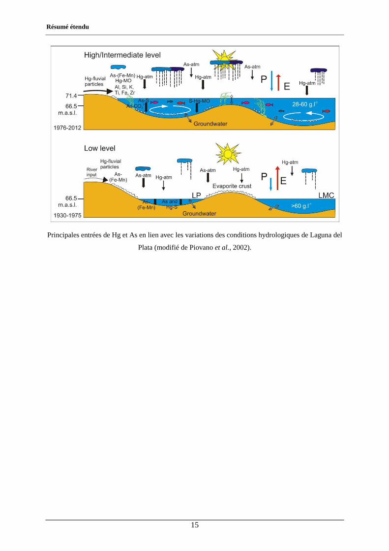
L’ensemble des résultats a permis de réviser le modèle hydro-géochimique proposé par
Piovano et al. (2002) en affinant davantage le fonctionnement de Laguna del Plata et en
incluant les phases porteuses principales de Hg et As identifiées dans la région.
Dans la figure, les précipitations (P) et l'évaporation (E) sont représentées par des flèches dont
la longueur est proportionnelle au volume. Le ruissellement de la rivière, qui s’est intensifié à
partir des années 1970, est indiqué par une flèche pleine. En revanche, la flèche apparait en
pointillés lorsque les débits de la rivière deviennent faibles, conditions hydrologiques qui
prédominent durant la période sèche. L'épaisseur des flèches, associées à différentes phases
du Hg et As étudiées dans la région, est proportionnelle à l’importance de leurs flux
respectifs. Avant les annés 1970, la période sèche domine et s´accompagne de niveaux des
lacs bas. Les entrées de Hg dans le lac provenaient alors principalement de sources naturelles
comme le mercure associé aux particules (notamment aux sulfures) qui ont été transportées
vers le lac depuis la partie supérieure du bassin de la rivière Suquía ou encore le Hg
atmosphérique (dépôt sec). Dans des conditions de hautes eaux (après 1970), ces deux sources
ont augmenté leurs contributions en raison d’une augmentation des précipitations (dépôt
Résumé étendu
14
humide) et de l'érosion des sols dans la partie supérieure du bassin versant mais aussi de
l'augmentation globale du flux de Hg dans l’atmosphère. Les conditions plus humides
entraînent une augmentation de la production primaire du lac et donc une plus grande affinité
du Hg pour la matière organique particulaire qui se trouve dans les sédiments accumulés au
cours de cette période.
En revanche, l'arsenic est principalement associé aux (hydr)oxydes de Mn et Fe dans la phase
aqueuse, ceci étant favorisé par les conditions de pH élevé du lac en basses et hautes eaux. En
outre, dans des conditions plus sèches, l'entrée de l’As dans le lac a été renforcée par les vents
dominants qui ont porté les particules de lœss riches en cet élément. Dans des conditions plus
humides, l'entrée d’As depuis l'atmosphère devient moins important et il est surtout présent
dans le lac associé aux particules provenant de la rivière. En plus d'être associé aux
(hydr)oxydes de Mn et Fe, l’As est associé à la pyrite dans la partie inférieure de la carotte
sédimentaire et à la calcite dans les parties médiane et supérieure. Par ailleurs, l'arsenic
résiduel qui ne peut pas être expliqué par les extractions sélectives peut être fixé sur la pyrite
non réactive.
Les sources de Hg et d'As dans les sédiments de Laguna del Plata sont le plus souvent
attribuées à des sources naturelles. Dans le cas du Hg, une contribution des flux mondiaux
devrait être considérée ainsi que de certaines autres sources anthropiques locales. Ces
dernières sont devenues de plus en plus importantes à partir des années 1970 suite au
développement industriel de la région. L'activité volcanique qui a eu lieu au début des années
1990 aurait pu également augmenter le signal du Hg. En ce qui concerne l'As, l'entrée
principale est clairement associée à la contribution croissante des particules lœssiques pendant
la période sèche qui a régné dans la région avant les années 1970.
Résumé étendu
15
Principales entrées de Hg et As en lien avec les variations des conditions hydrologiques de Laguna del
Plata (modifié de Piovano et al., 2002).

Table of content
17
Table of content ACKNOWLEDGEMENT .................................................................................................... 3
RESUME ....................................................................................................................... 7
ABSTRACT ...................................................................................................................... 9
RESUME ETENDU .......................................................................................................... 11
TABLE OF CONTENT ..................................................................................................... 17
L IST OF FIGURES .......................................................................................................... 19
L IST OF TABLES ............................................................................................................ 23
INTRODUCTION ............................................................................................................ 25
1. REGIONAL CONTEXT OF LAGUNA MAR CHIQUITA AND LAGUNA DEL PLATA .... 29
1.1 Location ................................................................................................................................ 31
1.2 Regional Climate .................................................................................................................. 35
1.2.1 Modern Climate ............................................................................................................... 35
1.2.2 Paleoclimate..................................................................................................................... 37
1.3 Vegetation ............................................................................................................................. 39
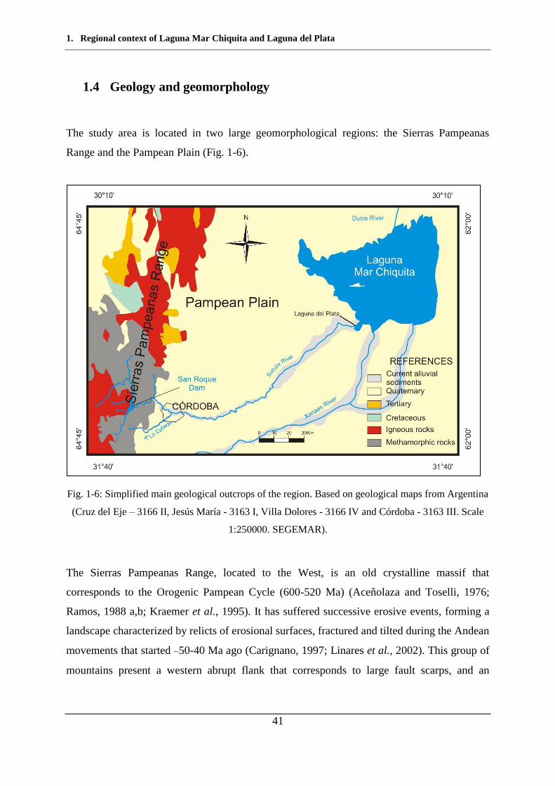
1.4 Geology and geomorphology ............................................................................................... 41
1.5 Sources of modern sediments .............................................................................................. 44
1.6 Water Mass Circulation and Hydrological modelling ...................................................... 45
1.7 Paleolimnology ..................................................................................................................... 52
2. HAZARDOUS ELEMENTS IN THE ENVIRONMENT : MERCURY AND ARSENIC ........ 57
2.1 Mercury ................................................................................................................................ 59
2.1.1 Mercury in the environment ............................................................................................ 59
2.1.2 Global Mercury Cycle ..................................................................................................... 60
2.1.3 Dynamics of Hg ............................................................................................................... 64
2.1.4 Mercury sedimentation .................................................................................................... 66
2.1.5 Mercury in the world and Argentina ............................................................................... 68
2.2 Arsenic .................................................................................................................................. 71
2.2.1 Arsenic in the environment .............................................................................................. 71
2.2.2 Sources of Arsenic ........................................................................................................... 72
2.2.3 Arsenic in natural waters ................................................................................................. 74
2.2.4 Arsenic in the world and in Argentina ............................................................................. 77
3. MATERIALS AND METHODS ..................................................................................... 83
3.1 Sampling campaigns and samples treatment .................................................................... 85
3.1.1 Water and sediment samples ........................................................................................... 86
3.1.2 Sediment core .................................................................................................................. 88
3.2 Analytical Methods .............................................................................................................. 90
3.2.1 Core dating – Radionuclides ............................................................................................ 90
3.2.2 Selective extractions ........................................................................................................ 92
3.2.3 Mineral characterization .................................................................................................. 95
Table of content
18
3.2.4 Chemical characterization ............................................................................................... 98
3.2.5 Summary ........................................................................................................................ 105
3.3 Satellite Image treatment .................................................................................................. 106
3.3.1 Contributions of satellite images ................................................................................... 106
3.3.2 Image treatment with ArcGIS ........................................................................................ 110
4. RESULTS ................................................................................................................. 115
4.1 Geochemical characterization of the basin ...................................................................... 117
4.1.1 Aquatic geochemistry .................................................................................................... 117
4.1.2 Trace metal concentrations ............................................................................................ 122
4.1.3 Aquatic geochemistry of As .......................................................................................... 125
4.1.4 Mineralogy of sediments and lake bottom sediments .................................................... 126
4.1.5 Hg in riverbed and lake bottom sediments .................................................................... 127
4.2 Geochemical and sedimentological characterization of the sedimentary record in Laguna del Plata ........................................................................................................... 129
4.2.1 Textural, physical and chemical properties of the sediments ........................................ 129
4.2.2 Physicochemical properties ........................................................................................... 134
4.2.3 Core dating: age model .................................................................................................. 136
4.2.4 Mineralogical and chemical composition of the LP core sediments ............................. 138
4.2.5 Total Particulate Mercury (HgTP) and solid speciation .................................................. 141
4.2.6 Total Particulate arsenic (AsTP) and solid speciation ..................................................... 145
4.3 Accumulation rates of Hg and As ..................................................................................... 147
4.4 Quantification of the size variation of Laguna Mar Chiquita and Laguna del Plata Lake system ................................................................................................................... 151
4.4.1 Laguna Mar Chiquita ..................................................................................................... 152
4.4.2 Laguna de Plata ............................................................................................................. 153
4.5 Summary ............................................................................................................................. 157
5. DISCUSSION ............................................................................................................ 159
5.1 The hydrogeochemistry of the Suquía River basin ......................................................... 161
5.2 The geochemistry of riverbed sediments in the Suquía basin ........................................ 163
5.3 Chronology and sediment deposition of the sedimentary core ...................................... 164
5.4 The historical record of Hg and As in sediments accumulated in Laguna del Plata during the last ~80 years ............................................................................................... 168
5.4.1 Mercury ......................................................................................................................... 168
5.4.2 Arsenic ........................................................................................................................... 171
6. CONCLUSION .......................................................................................................... 173
6.1 Perspectives ........................................................................................................................ 178
BIBLIOGRAPHY ........................................................................................................... 179
ANNEXES ................................................................................................................... 209
List of figures
19
List of figures
Fig. 1-1 : Study area location. (Modified from Piovano et al., 2006 and Troin et al., 2010) ................................ 33
Fig. 1-2 : Laguna Mar Chiquita size variations in 40 years through aerial pictures and satellite images; a)
Bucher et al., 2006, b) INPE Brazil, c) and d) Troin et al., 2010, e) to l) CONAE,
http://catalogos.conae.gov.ar ....................................................................................................................... 34
Fig. 1-3: Main climatic features that operate in Southern America. ITCZ: Inter Tropical Convergence Zone,
SALLJ: South American Low-Level Jet, SACZ: South Atlantic Convergence Zone and westerly belt
south of 35°S. (Adapted from Garreaud, 2009 and Zular et al., 2013) ........................................................ 36
Fig. 1-4: Climatic fluctuations in the Central Region of Argentina during the last 1000 years (Cioccale,
1999). ........................................................................................................................................................... 38
Fig. 1-5: Scheme profile of the typical landscape and vegetation variation from the borders of Mar Chiquita
depression to Dulce River channel, close to its mouth in the lake. (From Menghi, 2006). ......................... 39
Fig. 1-6: Simplified main geological outcrops of the region. Based on geological maps from Argentina (Cruz
del Eje – 3166 II, Jesús María - 3163 I, Villa Dolores - 3166 IV and Córdoba - 3163 III. Scale
1:250000. SEGEMAR). ............................................................................................................................... 41
Fig. 1-7: Main geomorphological and tectonic features that characterize the region (Modified from Mon and
Gutierrez, 2009 and Kröhling and Iriondo, 1999). ...................................................................................... 43
Fig. 1-8: Depositional regions in the bottom of Laguna Mar Chiquita (modified from Martinez et al., 1994
and Kröhling and Iriondo 1999). ................................................................................................................. 44
Fig. 1-9: Laguna Mar Chiquita bathymetry between levels 61 and 72 m.a.s.l (Pozzi et al., 2005). Red colours
corresponds to the deepest area and blue ones to the shallowest. ................................................................ 47
Fig. 1-10: Schematic diagram of the main components treated in the Lambda 2 model. QRD: Dulce River
input; QR: Dulce River input at the wetlands entry; QB: Wetlands input to the lake; QS+QX: Suquía
and Xanaes Rivers input (Modified from Rodriguez et al., 2005). ............................................................. 48
Fig. 1-11: Water flow directions in Laguna del Plata from COHERENS Model in the a) superficial, b)
middle and c) bottom layers (Modified from Corral et al., 2005). .............................................................. 51
Fig. 1-12: Age 210Pb profile and sedimentation rates for high and low stands, obtained from the slope of the
best-fit linear equation. ASR, average sedimentation rate for the entire dated interval (Piovano et al.,
2002). ........................................................................................................................................................... 53
Fig. 1-13: Model that represents lake level variations and the associated sedimentary record. Arrows indicate
Precipitation (P) and Evaporation (E) balance; their relative lengths indicate the predominance of P or
E. Higher river runoff and groundwater inputs are indicated in solid arrows and lower inputs are
indicated in dotted arrows (from Piovano et al., 2002). .............................................................................. 56
Fig. 2-1: Left: metallic mercury (crfzoraida.blogspot.fr) and right: cinnabar (HgS) from Almadén, Cuidad
Real, Spain (http://wwwblogmylcom.blogspot.fr/) ..................................................................................... 60
List of figures
20
Fig. 2-2: A recent estimate of the fluxes of mercury at the Earth’s surface based on simulations using the
GEOS-Chem global mercury model. The percentage values in brackets are the estimated increases in
concentration and fluxes in the last century due to anthropogenic activities (Mason et al., 2012). ............ 61
Fig. 2-3: Schema showing the heterogeneous chemistry influencing the wet deposition of Hg. (Modified
from Lindqvist et al., 1991) ......................................................................................................................... 65
Fig. 2-4: Cycle of Hg. Reactions, transformations and transfers (hum = humic acid; SR-b = sulfate-reducing
bacteria; FeR = iron-reducing bacteria). Modified from Castelle, 2008. ..................................................... 67
Fig. 2-5: Arsenic minerals. Left image, Arsenopyrite - FeAsS (http://wisconsingeologicalsurvey.org), middle
image, Orpiment - As2S3 (www.volcanol.fr) and right image, Realgar – AsS (http://webmineral.com). .... 71
Fig. 2-6: Arsenic distribution of documented world problems whether they are related to aquifers or mining
(red dots) and geothermal (green dots) sources (Smedley and Kinniburgh, 2002)...................................... 77
Fig. 2-7: Picture of the volcanic glass typically found in the Chaco-Pampean Plain loess (Francisca and
Carro Perez, 2009). ...................................................................................................................................... 80
Fig. 3-1: Sampling points on the Suquía River and its catchment area and lakes Laguna del Plata and Laguna
Mar Chiquita................................................................................................................................................ 85
Fig. 3-2: Water and sediment sampling – a) Collecting samples from the river, b) Collecting samples from
the lakes using a Van Dorn bottle. ............................................................................................................... 87
Fig. 3-3: LP Core – a and b) Extraction of the sediment core using a manual Eijkelkamp core sampler type
Beeker, c) Core photograph, d) X-ray SCOPIX High-resolution image. .................................................... 89
Fig. 3-4: Laser granulometer equipment. Malvern Mastersizer S (Malvern Mastersizer, 1997). ......................... 96
Fig. 3-5: Total and Organic Carbon analysis – a) Treated samples with HCl and b) LECO device ..................... 99
Fig. 3-6: Schematic sampling processing system of DMA equipment (adapted from
http://www.milestonesrl.com). .................................................................................................................. 101
Fig. 3-7: Direct Mercury Analyzer (DMA) 80 MILESTONE – a) Analyzer device, b) Auto-sampler tray, c)
Read-out terminal. ..................................................................................................................................... 102
Fig. 3-8: Flow Injection Atomic Absorption Spectrophotometry, a) Schematic operation diagram of FIAS
300 (modified from Hineman, 2011) b) Measurement equipment at EPOC laboratory. ........................... 104
Fig. 3-9: Electromagnetic spectra and Remote Sensing System adapted from Girard and Girard (2010). ......... 108
Fig. 3-10: Differences in contrast between bands 3 (a) and 5 (b) of a same satellite image from December
25th, 2000. .................................................................................................................................................. 110
Fig. 3-11: Raster of band 5 showing the training fields (a) and (b) shows training fields already classified.
Class “water” corresponds to the polygons in blue and “land” ones those in green. ................................. 111
Fig. 3-12: a) Thematic map produced by Maximum Likelihood classification. Blue represents water and
green represents land that includes the “rest” besides water; b) Final image showing the main polygon
that contains Laguna Mar Chiquita............................................................................................................ 112
List of figures
21
Fig. 3-13: Image a) shows the location of LP and its respective mask in red, b) is the crop of the raster
generated by the mask and c) is the final polygon obtained for LP after the Maximum Likelihood
Classification. ............................................................................................................................................ 113
Fig. 4-1: Piper diagrams showing the chemical evolution of Suquía River waters and both lake waters. .......... 120
Fig. 4-2: Stiff diagrams showing the major chemical composition of water samples in the Suquía River and
in the lakes. Notice that the concentration scale in the X-axis is different for river and lake waters. ....... 120
Fig. 4-3: Arsenic concentrations in river waters with respect to the geographical position in the basin (RCQ2
to RSAcorrespond to headwaters). ............................................................................................................ 125
Fig. 4-4: XRD diffractograms for Suquía riverbed sediments (RS-7 and RS-8) and for Laguna del Plata (LP
11-6) and Laguna Mar Chiquita (TMC 11-1) bottom sediments. Ill: Illite, Ab: Albite, Qtz: Quartz, Mc:
Microcline, Prv: Perovskite, Py: Pyrite, Cal: Calcite, Hl: Halite, Bt: Biotite. ........................................... 126
Fig. 4-5: Distribution of Hg concentrations of the silty fraction in the basin. Concentrations are given in µg
kg-1 and the size of the circle corresponds to the amount of mercury measured at a certain point. ........... 128
Fig. 4-6: Gray and olive green colour scale corresponding to the SCOPIX X-ray image (a) and the
photograph (b). Letters A to E correspond to the Lamination Indexes (LI). ............................................. 131
Fig. 4-7: Grain size distribution for LP core samples. ........................................................................................ 133
Fig. 4-8: Physical parameters corresponding to LP core plotted next to Laguna Mar Chiquita Lake-level
(LMCL) variations, a) sediment core X-ray image, b) sediment core photograph, c) LMCL – Laguna
Mar Chiquita Lake-level, the dashed line corresponds to reconstructed data developed in Piovano et
al., 2002., d) pH values, e) porosity record expressed in percentage, f) Organic Carbon (Corg) content,
g) Inorganic Carbon (Cinorg) content, h) Sulphur (S) content. .................................................................... 135
Fig. 4-9: Core dating. (A) Normalized 210Pbxs against cumulative mass: the dashed line corresponds to the
exponential regression used to determine Mass Accumulation Rate (MAR). (B) Average
Sedimentation Rate (ASR) and (C) 137Cs plotted against calendar ages, based on 210Pb dating. ............... 137
Fig. 4-10: XRD diffractograms LP core sediments. Ms: Muscovite, Bt: Biotite, Kln: Kaolinite, Mnt:
Montmorillonite, Ab: Albite, Qtz: Quartz, Cal: Calcite, Hl: Halite, Py: Pyrite. ........................................ 139
Fig. 4-11: XRF logs from Laguna del Plata. The values are given in counts per second (cps). According to
their behaviour, LP core is separated into 3 main zones: from 120 to 74 cm, 74-16 cm and 16-0 cm. ..... 141
Fig. 4-12: Mercury concentrations. a) Selective extractions corresponding to the concentrations of total
particulate (HgTP), oxidisable ( ) and acid-soluble/reactive (HgHCl) fractions. Relations
between (b) and HgTP and (c) HgHCl and HgTP. ........................................................................... 143
Fig. 4-13: Fe (a) and Mn (b) determinations in the supernatants of HCl and Asc. ............................................. 144
Fig. 4-14: Arsenic profiles along the LP core depth showing a) Total arsenic (Astotal), reducible (Asasc) and
acid-soluble/reactive (AsHCl) fractions. (b) Ratios of Asasc/Astotal and (c) AsHCl/Astotal. ............................. 145
Fig. 4-15: Comparison between a) As-HCl fraction, b) Cinorg along the sedimentary core, c) Laguna Mar
Chiquita Lake-level variations (LMCL) and d) Ca/As molar ratio. .......................................................... 146
Fig. 4-16: Relationship between Fe and As and Mn and As measured in the ascorbate (asc) fraction. .............. 147
List of figures
22
Fig. 4-17: a) LMCLL – Laguna Mar Chiquita Lake-level variations, b) Accumulated mass for Hg for HgTP, and HgHCl fractions, c) Hg fluxes and d) Accumulated mass for Corg. ....................................... 148
Fig. 4-18: a) Accumulated mass for As for Astot, HgHCl and Hgasc fractions, b) As fluxes .................................. 151
Fig. 4-19: Size variation of Laguna Mar Chiquita. The biggest size corresponds to the year 2003 while the
smallest one to 2013 in the period that spans from September 1988 to June 2013. .................................. 153
Fig. 4-20: Size variation of Laguna de Plata The biggest size corresponds to the year 2003 while the smallest
one to 2013 in the period that spans from September 1988 to June 2013. The black dot corresponds to
the emplacement of LP core. ..................................................................................................................... 154
Fig. 4-21: Chronological size variation of Laguna del Plata compared to the variation of the lake-level of
Laguna Mar Chiquita and the precipitation record of the Miramar town. ................................................. 156
Fig. 5-1: Salt storm over Mar Chiquita System on September 15th, 2013 (NASA). ........................................... 166
Fig. 6-1: Main mineralogical inputs related to hydrological variations in Laguna del Plata. Adjusted from
Stupar et al. (2013) .................................................................................................................................... 176
List of tables
23
List of tables
Table 1-1: Necessary Dulce River discharge to keep the different Laguna Mar Chiquita levels and the
estimated salinity in each case (Rodriguez et al., 2005). ............................................................................. 48
Table 2-1: Typical Hg concentrations in rocks, soils and sediments around the world. * Volcanic Influence,
** Mining influenced. ................................................................................................................................. 70
Table 2-2: Typical As concentrations in natural waters, rocks and sediments around the world (Smedley and
Kinniburgh, 2002). * Groundwater influenced, ** Geothermal influenced, *** Mining influenced. ........ 78
Table 3-1: List of sample type, analysis and method used for this work. ........................................................... 105
Table 3-2: Main characteristics for Landsat 5, 7 and 8 bands. * TM Band 6 was acquired at 120-meter
resolution, but products processed before February 25, 2010 are resampled to 60-meter pixels.
Products processed after February 25, 2010 are resampled to 30-meter pixels. ** ETM+ Band 6 is
acquired at 60-meter resolution. Products processed after February 25, 2010 are resampled to 30-meter
pixels. ***Information that corresponds to Landsat 8 (http://landsat.usgs.gov). ...................................... 109
Table 4-1: Physicochemical parameters of river and lake water samples. Cond. – Conductivity, TDS – Total
Dissolved Solids. Concentrations of major ions are expressed in meq L-1. IB: Ionic Balance, DO:
dissolved Oxigen nd: not determined. ....................................................................................................... 119
Table 4-2: Saturation indices calculated for water samples with PHREEQC. .................................................... 122
Table 4-3: Statistical summary for some selected trace elements in the Suquía River basin .............................. 123
Table 4-4: Arsenic concentrations on water samples in the Suquía River basin ................................................. 123
Table 4-5: Correlation matrix. Values 0.5 are in pale gray and those -0.5 in dark gray; TDS: Total
Dissolved Solids; nd: not determined. ....................................................................................................... 124
Table 4-6: Mercury concentrations on riverbed, lake bottom and pluviometric captor sediment samples
expressed in µg kg-1. .................................................................................................................................. 127
Table 4-7: Satellite images information and the calculated size and reduction. Satellite image in black
correspond to the maximum extension. ..................................................................................................... 155

Introduction
25
Introduction
In the central Argentina, the Chaco Pampean Plain is a vast loessic plain that extends from the
Andean Cordillera in the west to the Atlantic Ocean in the east. It covers an area of around
1x10⁶ km2 that represents ~36 % of the Argentinean territory. A series of lakes is found along
a N-S bar located in the eastern border of the plain (30°S to 37°S). The analyses of the
sediments accumulated in these lakes have shown high sensitivity to the climatic changes that
have occurred since the last Little Ice Age (LIA). The most conspicuous example is the Mar
Chiquita system is composed of the Laguna Mar Chiquita, Laguna del Plata and the Río
Dulce wetlands. During highstands, Laguna Mar Chiquita becomes not only the largest saline
lake in South America but also one of the largest in the world. Furthermore, the lake has
varied its size from ~6000 km2 in the wettest periods to the ~2000 km2 that shows nowadays
but it was even smaller with ~1000 km2 in the past (Piovano et al., 2009) when a dry climate
prevailed. In the southernmost margin of the Laguna Mar Chiquita, the Laguna del Plata is a
small lake that forms a bay with it during highstands (Oroná et al., 2010) and stays connected
through a small channel during lowstands. Laguna del Plata receives the runoff waters of the
Suquía River whose headwaters are located in the Sierras Pampeanas Range, in the west.
Most of these tributaries in the upper catchments are stored in the San Roque Dam
(31°22'13.43"S; 64°27'41.40"W, 643 m.a.s.l.). Downflow, the river crosses the city of
Córdoba and the loessic plain of the Chaco Pampean Plain, after travelling around 200 km.
Finally, the Suquía River discharges into the Laguna del Plata. This system is subject to a
growing urban and industrial development since the mid 20th Century that had probably
impacted in the chemistry of the river. Some authors (i.e., Pesce and Wunderlin, 2000;
Wunderlin et al., 2001; Monferrán et al., 2011; Pasquini et al., 2011) observed a decrease in
the water quality from pristine regions in the upper fluvial catchments to the proximity of the
lake. Gaiero et al. (1997) noticed increasing trace metal concentrations in riverbed sediments
downflow, which was attributed to the urban impact. At present there is no comprehensive
data on the long-term change in metal contents of the Suquía river sediment load.
The environmental evolution of a region can be well-recorded in the relatively stable
sedimentary environment (Oldfield and Appleby, 1984). Therefore, the study of the sediments
Introduction
26
accumulated in lakes has a great importance for the analysis of the environmental processes,
based on a detailed and accurate 210Pb chronology (Sanchez-Cabeza et al., 2000).
In the present study, the historical records of two contaminants were analyzed in the
sediments accumulated in the last 80 years in the Laguna del Plata, with the aim of
identifying their variability with the hydrological and climatic conditions predominant in the
last 80 years in the northern Chaco Pampean region. On one hand, a typical atmospheric-
borne element such as Hg was selected due to its already documented sensibility to global
changes. On the other hand, a geogenic contaminant such as arsenic, whose presence has been
largely reported in the Chaco Pampean region is analyzed focusing on its geochemical
behaviour under alternating saline and freshwater conditions.
The hypothesys of the present work are:
- The climate variations in the Mar Chiquita system have influence on its chemical
composition, and particularly on the dynamics of the studied trace elements
- Hg sources are likely associated with the global flow of this element,
- The record of As in the lake sediments likely responds to the variable contributions
from the loessic sediments that cover the Chaco Pampean Plain
- The volcanic eruptions in the Andes Cordillera are a potential source of trace elements
(such as Hg) that accumulate in the sedimentary record of the Mar Chiquita system.
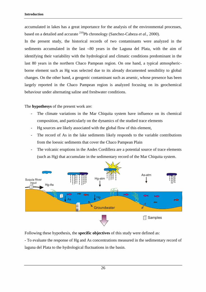
Following these hypothesis, the specific objectives of this study were defined as:
- To evaluate the response of Hg and As concentrations measured in the sedimentary record of
laguna del Plata to the hydrological fluctuations in the basin.
Introduction
27
- To contribute to a better knowledge of the spatial distributions of mercury and arsenic in the
basin,
- To analyze the variability of their concentrations in the sediments accumulated in the past 80
years,
- To identify their sources and dynamics during transport and accumulation,
To achieve these objectives, a large set of geochemical, isotopic, hydrological and
limnogeologial tools were used.
The approach to achieve these objectives is outlined in the six parts of this thesis.
First chapter:
It provides the information to place the study area into its geographical context. It allows as
well to understand the climatic features that triggered the climate changes and the geo-
physicochemical consequences over the Mar Chiquita system.
Second chapter
This chapter contains general information about the occurrence of Hg and As in the
environment. Primary sources, dynamics, chemical associations and previous works in the
world and Argentina are discussed.
Third chapter
In this chapter, all methodological aspects are described. Details of the sampling
methodology, analytical methods for water and sediment analysis, selective extractions,
determination of sediment´s mineralogy, core dating and satellite image interpretation are
included.
Fourth chapter
It presents all the results obtained. For a better understanding the results show firstly the
information obtained in the Suquía River basin and its spatial distribution. Secondly, the
results corresponding to the sedimentary core that give the temporal distribution are
presented.
Introduction
28
Fifth chapter
The results presented in the previous chapter are interpreted and discussed.
Sixth chapter
Finally, a hydro-geochemical model for the Mar Chiquita system including Hg and As
bearing phases is described as well as the perspectives of this work.
1. Regional context of Laguna Mar Chiquita and Laguna del Plata
29
1. Regional context of Laguna Mar
Chiquita and Laguna del Plata
1. Regional context of Laguna Mar Chiquita and Laguna del Plata
30
1. Regional context of Laguna Mar Chiquita and Laguna del Plata
31
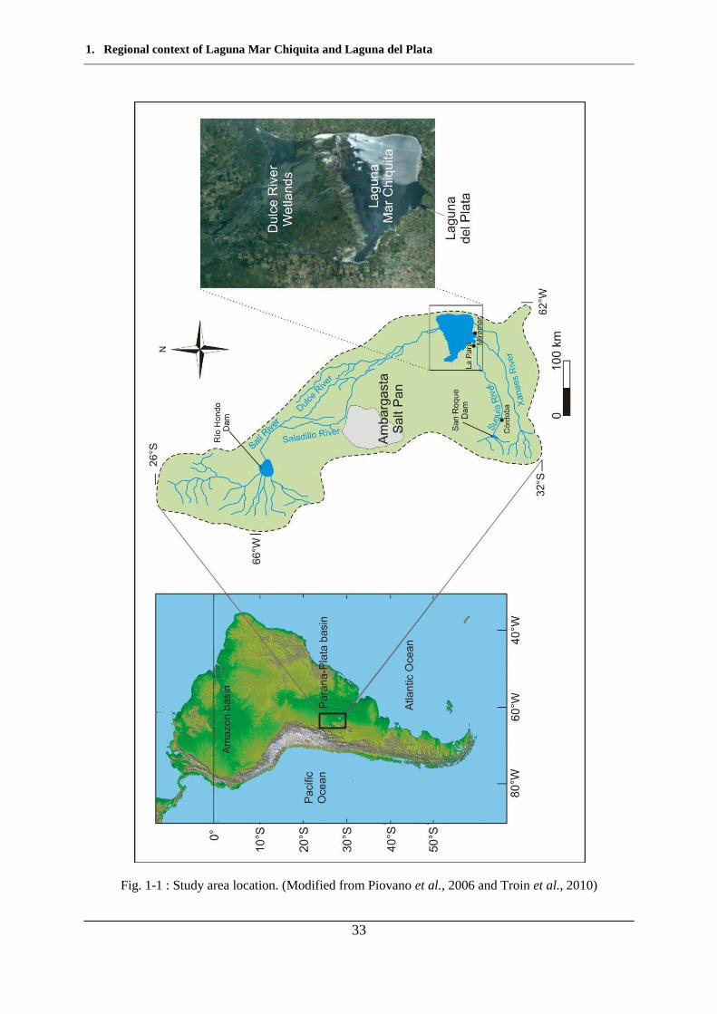
1.1 Location
Laguna Mar Chiquita system (Laguna Mar Chiquita, Laguna del Plata and the Dulce River
wetlands) is located in the provinces of Córdoba and Santiago del Estero occupying a vast
area that goes between 26° to 31° S and 62° to 63°’ W in the geological province of the Chaco
Pampean Plain. The system plays an important biological role due to its rich and abundant
biodiversity as well as anthropological interest to the point that was declared a Ramsar site by
the United Nations (http://ramsar.wetlands.org).
The Laguna Mar Chiquita system catchment covers an area of around 127,000 km2 (Fig. 1-1).
At the present time, there are three rivers that flow into the lake: The Suquía, Xanaes and
Dulce Rivers.
- The Suquía River (200 km) headwaters are located in the Sierras Pampeanas de
Córdoba (between 29°00' - 33°30'S and 64°00' - 65°30'W) where different mining activities
(mainly rock quarries) and land-use have been developed. The San Roque reservoir
(643 m.a.s.l. - 31°22 41 S, 64°28 10 W) located upstream from Córdoba city, collects the
waters from the catchment’s tributaries and is used for flood control and drinking water
reservoir. Downflow, the river crosses from west to east of the city of Córdoba which is the
second biggest of Argentina (1.3 million inhabitants) after Buenos Aires. Automobile
industry, machinery manufacturing, food and paint production are the main economical
activities in the city. In its lower stretch, the Suquía River crosses the loessic depression of the
Chaco Pampean Plain (Zárate, 2003) which is one of the most important agricultural areas of
the country. Finally the river discharges into the Laguna del Plata situated in the South West
margin of the Laguna Mar Chiquita and connects to it during high lake-level periods.
- The Xanaes River (300 km) has its headwaters also in the Sierras Pampeanas
Range and originates in the confluence of the Anizacate and Los Molinos rivers. In the Chaco
Pampean plain, it runs with a W-E direction (Vázquez et al., 1979) parallel to the Suquía
River until reaching Laguna Mar Chiquita.
- The Dulce River (812 km) is the most important of the three rivers owed to its
volume. Its headwaters are located in the limit between the provinces of Salta and Tucumán
(NW region of Argentina). After 100 kilometres the river discharges into the Río Hondo Dam
(27°31'34.76"S; 64°58'37.65"W with an extension of 330 km2 at ~350 m.a.s.l.) and a few
1. Regional context of Laguna Mar Chiquita and Laguna del Plata
32
kilometres downflow the output it divides into two branches. One of them (Saladillo River)
crosses the Ambargasta salt pan raising the salinity of its waters and binds anew to the Dulce
River. Finally, the highly saline river flows into the Laguna Mar Chiquita (Vázquez et al.,
1979) from its northern coast.
The combined average annual discharge of both Suquía and Xanaes Rivers is 725 hm3 while
the discharge of Dulce River ascends to 2996 hm3 (Reati et al., 1997).
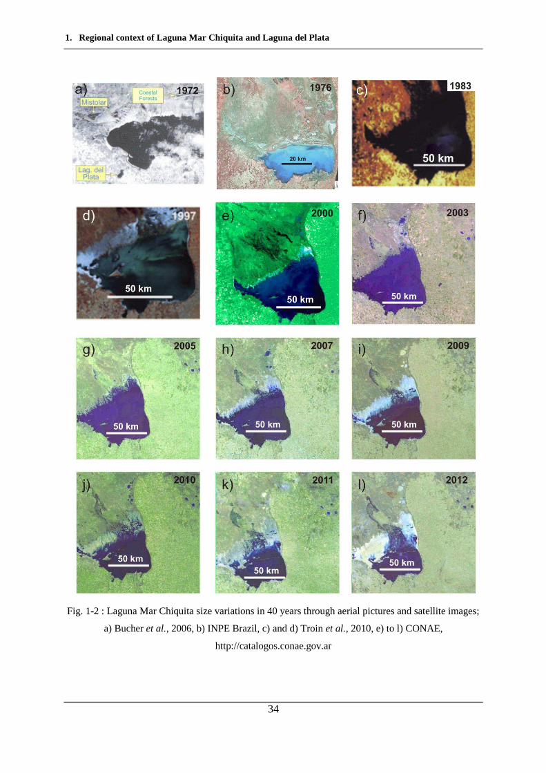
Several authors (e.g., Kröhling and Iriondo, 1999; Piovano et al., 2002; Bucher et al., 2006;
Leroy et al., 2010) have mentioned the dramatic lake levels fluctuations that Mar Chiquita has
suffered all along its history. These hydrological fluctuations are evident not only through the
sedimentary record, but also through the continuous variations of lake area registered in the
last 30 years by satellites images (Fig. 1-2). Laguna Mar Chiquita is the largest saline lake in
South America and one of the biggest in the world (Piovano et al., 2002, 2004a,b). It reached
its maximum level (71.4 m.a.s.l.) in 2003 with an extension of ~6500 km2. At the moment of
this work, Laguna Mar Chiquita shows a reduction in its area of ~50 % reaching an extension
of ~2220 km2 and a lake-level of 68.1 m.a.s.l. Bucher et al. (2006) divided this area in two
sub-regions: the Dulce River wetlands which include a series of small lakes located in the NE
part of the Laguna Mar Chiquita and the present channel of the Dulce River. The landscape is
characterised by a plain covered with scrub vegetation that is intentionally burnt twice a year
to improve the palatability for the cattle. The other region is the one occupied by the actual
Laguna Mar Chiquita.
On the east side, the lake is limited by the San Guillermo high lifted up by the Tostado-Selva
fault (Mon and Gutierrez, 2009). The southern margin is a potentially flooded depression cut
by some remaining sandy elevations formed during the past driest periods. Farming and cattle
are the main economic activities in this area. The eastern flanks of the Sierras Pampeanas
foothills reach the western margin of the Mar Chiquita Lake, where agricultural expansion
produced an elevated deforestation. Finally, the North shore is characterised by the presence
of muddy and salty playas derived from the intense hydrological fluctuations that affect the
region.
1. Regional context of Laguna Mar Chiquita and Laguna del Plata
33
Fig. 1-1 : Study area location. (Modified from Piovano et al., 2006 and Troin et al., 2010)
1. Regional context of Laguna Mar Chiquita and Laguna del Plata
34
Fig. 1-2 : Laguna Mar Chiquita size variations in 40 years through aerial pictures and satellite images;
a) Bucher et al., 2006, b) INPE Brazil, c) and d) Troin et al., 2010, e) to l) CONAE,
http://catalogos.conae.gov.ar
1. Regional context of Laguna Mar Chiquita and Laguna del Plata
35
1.2 Regional Climate
1.2.1 Modern Climate
South American climate is complex and exhibits tropical, subtropical and extratropical
climatic features that extent from 10°N to 53°S (Garreaud et al., 2009). These authors have
well summarized the present-day South American climate where significant differences are
given at both sides of the Andes Cordillera that acts as a meridional topographic barrier
controlling the diversity of precipitation, temperature and wind patterns (Garreaud, 2009).
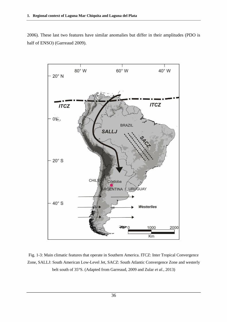
A major characteristic of the seasonal climate variability in South America is the occurrence
of a monsoon-like system (Vera et al., 2006) that extends southward from the tropical
continental region during the austral summer. It connects the Atlantic Inter Tropical
Convergence Zone (ITCZ) with the South Atlantic Convergence Zone (SACZ) by means of a
large-scale atmospheric circulation containing a low-level jet (Fig. 1-3). The South American
Low-Level Jet (SALLJ) starts in the northern part of South America at the foot of the Andes
and, driven by the Chaco Low, provides moisture to South Eastern South America (SESA)
(Nogués-Paegle and Mo 1997; Labraga et al. 2000) and basically determines the hydrological
balance of the region (Berbery and Collini 2000; Saulo et al. 2000; Berbery and Barros 2002).
Summer precipitation maxima and dry winters (in the Southern Hemisphere) characterize a
large area east of the Andes, between 22º S and 40º S, where the only external sources of
water vapour are the tropical latitudes and the south Atlantic Ocean (Doyle and Barros, 2002).
During austral summer, light easterly flow extends down to 21º S and the subtropical westerly
jet weakens and reaches its southernmost position. In contrast, during austral winter the
easterly winds are restricted to the north of 10º S and the subtropical westerly jet becomes
stronger with its core at 30º S (Garreaud, 2009). The westerlies act as a largely symmetric belt
south of 35°S due to the absence of significant land masses at these latitudes (Garreaud et al.
2009). Other important climatic features are the sporadic incursions of polar air outbreaks
(Antarctic Oscillation – AAO) east of the Andes (Marengo and Rogers 2001; Garreaud et al.
2009), the Pacific Decadal Oscillation (PDO) and ENSO (El Niño-Southern Oscillation)
teleconnections controlling precipitation and, hence, the hydrology of major riverine systems
(Aceituno 1988; Depetris et al. 1996; Silvestri 2004; Boulanger et al. 2005; Pasquini et al.,
1. Regional context of Laguna Mar Chiquita and Laguna del Plata
36
2006). These last two features have similar anomalies but differ in their amplitudes (PDO is
half of ENSO) (Garreaud 2009).
Fig. 1-3: Main climatic features that operate in Southern America. ITCZ: Inter Tropical Convergence
Zone, SALLJ: South American Low-Level Jet, SACZ: South Atlantic Convergence Zone and westerly
belt south of 35°S. (Adapted from Garreaud, 2009 and Zular et al., 2013)
1. Regional context of Laguna Mar Chiquita and Laguna del Plata
37
1.2.2 Paleoclimate
Paleoenvironmental evolution of the Late Pleistocene and Holocene (last 13.0 ka) for
Southern South America and east of the Andes was reconstructed by Piovano et al. (2009).
Concerning Laguna Mar Chiquita system, several authors (Piovano et al., 2004a,b, 2009)
consider it as a “sensitive hydroclimatic indicator” in South America mid-latitudes due to its
sharp lake-level fluctuations. The paleoclimate reconstruction was performed taking into
account limnogeological features observed in sedimentary cores retrieved from Laguna Mar
Chiquita, interpretation of satellite images, meteorological records, historical sources and
fieldwork. According to Piovano et al. (2009), the hydroclimatic record indicates positive
hydrological balance and therefore highstand onset at ca. (circa) 13.0 cal ka BP (calibrated
thousand years Before Present). This period was followed by extremely dry conditions that
triggered the precipitation of evaporates and more positive isotope composition of carbonates
and organic matter. After 6.8 cal ka BP there was an increase in the temperature gradient as a
result of an enhanced influence of the Southeast Pacific anticyclone, larger Antarctic sea-ice
extend (Gilli et al., 2005) and the effect of changes in insolation (Markgraf, 1998) that
derived on the strengthening of the Southern Westerlies. The most intense magnitude was
dated around 4.7 cal ka BP, this cold and dry phase of the Middle Holocene is consistent with
a reduced latitudinal convey of moisture from the tropics to the subtropics as a consequence
of a weakened Monsoonal circulation. These conditions extended until the middle of the first
millennia when less extreme lowstands can be inferred by 1.5 cal ka BP. The timing of the
droughts for the first and second millennia is poorly resolved due to the occurrence of several
sedimentary hiatuses indicated by gypsum-halite layers. Several climatic indicators suggest
that warm and humid conditions prevailed from 1400-800 y BP in the Central Region of
Argentina known as “Medieval Warm Period (MWP)” (Kröhling and Iriondo, 1999), that
allowed soil development and expansion of fluvial and lacustrine systems. This heating (Fig.
1-4) is explained as an enhancement of the South Atlantic Anticyclone (Cioccale, 1999). The
“Little Ice Age (LIA)” characterized by cold conditions started around 1300 (Cardich, 1980).
The LIA was not a homogeneous event; it was formed by two cold pulses separated by an
intermediate period of more benign conditions. The first cold pulse extended from the first
decades of the 15th Century until the end of the 16th Century. The intermediate period began at
1. Regional context of Laguna Mar Chiquita and Laguna del Plata
38
the end of the 16th Century and was prolonged until the beginning of the 18th Century
(Cioccale, 1999). From ~1770 sedimentation is more constant and was dated by 210Pb
(Piovano et al., 2002) indicating less extreme conditions with the occurrence of short-lived
humid pulses during the second half of the 19th Century (1850-1870) (Piovano et al., 2009).
Finally, the second cold pulse spanned from the beginning of the 18th Century until the
beginning of the 19th Century being the coldest part of the LIA and where the southern Andes
glaciers reached their maximum extension (Cioccale, 1999).
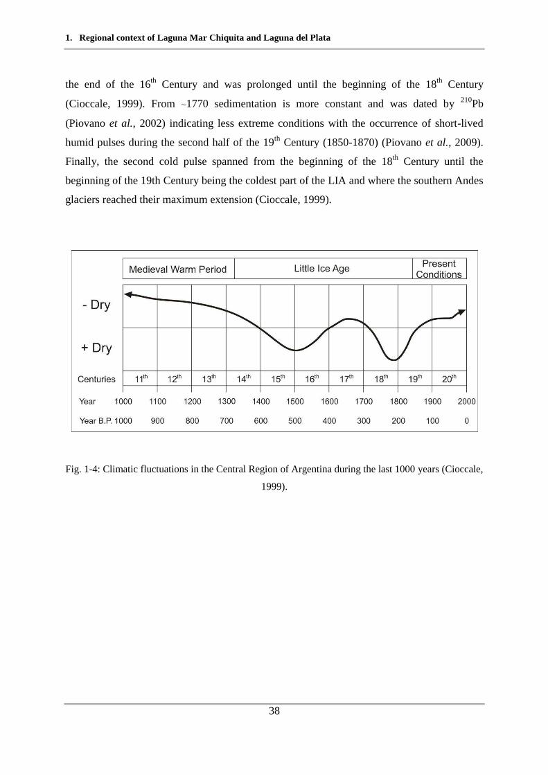
Fig. 1-4: Climatic fluctuations in the Central Region of Argentina during the last 1000 years (Cioccale,
1999).
1. Regional context of Laguna Mar Chiquita and Laguna del Plata
39
1.3 Vegetation
The diversity and spatial distribution of vegetation in the study area are determined by the
interaction between the landscape and the hydrology. The size of vegetation decreases with
increasing water table influence and soil salinity. The correspondence between vegetation and
the hydro-topographic gradient varies as follow: chaco forest (characterized by Aspidosperma
quebracho-blanco, Ziziphus mistol and Prosopis spp.) ➞ transition shrubland ➞ halophytic
scrub ➞flooded savanna (pajonal ➞ reed bed ➞ totoral➞ prairie). This spatial variation is
manifested along the Dulce River (Fig. 1-5) (Menghi et al., 2006).
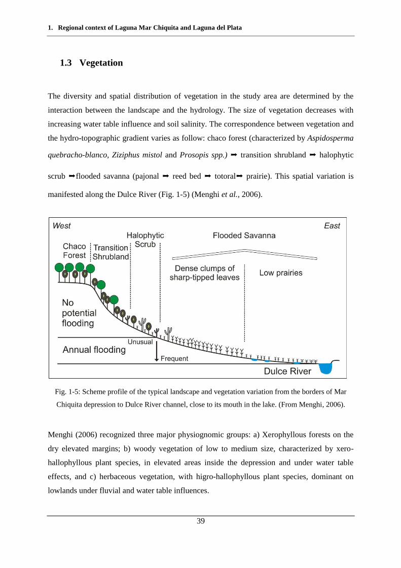
Fig. 1-5: Scheme profile of the typical landscape and vegetation variation from the borders of Mar
Chiquita depression to Dulce River channel, close to its mouth in the lake. (From Menghi, 2006).
Menghi (2006) recognized three major physiognomic groups: a) Xerophyllous forests on the
dry elevated margins; b) woody vegetation of low to medium size, characterized by xero-
hallophyllous plant species, in elevated areas inside the depression and under water table
effects, and c) herbaceous vegetation, with higro-hallophyllous plant species, dominant on
lowlands under fluvial and water table influences.
1. Regional context of Laguna Mar Chiquita and Laguna del Plata
40
Flooding and biomass fires are also system modellers. Periodic Dulce River flooding events
are vital to maintain soil fertility, habitats biodiversity, vegetation quality and productivity
(both livestock and floristic diversity purposes) and animal wildlife associated as well as
sediments deposition and removal, salt wash from the soils and nutrient inputs (Menghi et al.,
2001; Bucher and Bucher, 2006b). The second one (biomass fires) is frequent in flooded
savannas around the world (Whelan, 1995). The wet period that follows the floods favours the
production of grassland biomass and a grand majority dries at the end of the dry season
becoming highly flammable fuel. Under these conditions and even without human influence,
the grassland can easily burn due to solar rays (Bucher and Bucher, 2006b). The effect of the
biomass burning will depend on its intensity but there are some common patterns in the fire-
vegetation interaction. Fire does not allow woody vegetation expansion, favours grass
development and harms shrubberies and trees grow (Bucher and Bucher, 2006a). Biomass
burning liberates components by volatilization predominating greenhouse gasses and other
chemically active components such as carbon monoxide, nitric acid and sulphur oxides. At the
same time, fire mineralizes soil organic matter ions and as a consequence there is a rise in pH,
conductivity, calcium, magnesium, potassium, phosphorous, and ammonium values that could
last even one year after the burning (Schmalzer and Hinkle, 1992). In the burnt areas there is a
nude soil and an ash layer remaining that is easily removed by the water and wind and could
accumulate in Mar Chiquita (Bucher and Bucher, 2006b). Furthermore biomass burning is
increased by human activity even up to twice a year to control the growth of woody species
and promote the development of softer grasses that improve the palatability of the cattle
(Menghi et al., 2001; Bucher and Bucher, 2006b).
1. Regional context of Laguna Mar Chiquita and Laguna del Plata
41
1.4 Geology and geomorphology
The study area is located in two large geomorphological regions: the Sierras Pampeanas
Range and the Pampean Plain (Fig. 1-6).
Fig. 1-6: Simplified main geological outcrops of the region. Based on geological maps from Argentina
(Cruz del Eje – 3166 II, Jesús María - 3163 I, Villa Dolores - 3166 IV and Córdoba - 3163 III. Scale
1:250000. SEGEMAR).
The Sierras Pampeanas Range, located to the West, is an old crystalline massif that
corresponds to the Orogenic Pampean Cycle (600-520 Ma) (Aceñolaza and Toselli, 1976;
Ramos, 1988 a,b; Kraemer et al., 1995). It has suffered successive erosive events, forming a
landscape characterized by relicts of erosional surfaces, fractured and tilted during the Andean
movements that started ~50-40 Ma ago (Carignano, 1997; Linares et al., 2002). This group of
mountains present a western abrupt flank that corresponds to large fault scarps, and an
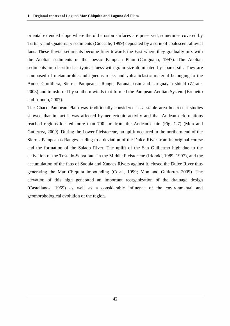
1. Regional context of Laguna Mar Chiquita and Laguna del Plata
42
oriental extended slope where the old erosion surfaces are preserved, sometimes covered by
Tertiary and Quaternary sediments (Cioccale, 1999) deposited by a serie of coalescent alluvial
fans. These fluvial sediments become finer towards the East where they gradually mix with
the Aeolian sediments of the loessic Pampean Plain (Carignano, 1997). The Aeolian
sediments are classified as typical loess with grain size dominated by coarse silt. They are
composed of metamorphic and igneous rocks and volcaniclastic material belonging to the
Andes Cordillera, Sierras Pampeanas Range, Paraná basin and Uruguayan shield (Zárate,
2003) and transferred by southern winds that formed the Pampean Aeolian System (Brunetto
and Iriondo, 2007).
The Chaco Pampean Plain was traditionally considered as a stable area but recent studies
showed that in fact it was affected by neotectonic activity and that Andean deformations
reached regions located more than 700 km from the Andean chain (Fig. 1-7) (Mon and
Gutierrez, 2009). During the Lower Pleistocene, an uplift occurred in the northern end of the
Sierras Pampeanas Ranges leading to a deviation of the Dulce River from its original course
and the formation of the Salado River. The uplift of the San Guillermo high due to the
activation of the Tostado-Selva fault in the Middle Pleistocene (Iriondo, 1989, 1997), and the
accumulation of the fans of Suquía and Xanaes Rivers against it, closed the Dulce River thus
generating the Mar Chiquita impounding (Costa, 1999; Mon and Gutierrez 2009). The
elevation of this high generated an important reorganization of the drainage design
(Castellanos, 1959) as well as a considerable influence of the environmental and
geomorphological evolution of the region.
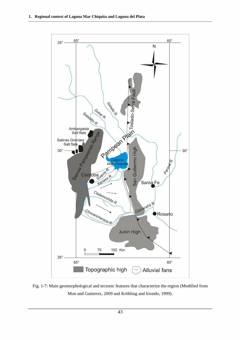
1. Regional context of Laguna Mar Chiquita and Laguna del Plata
43
Fig. 1-7: Main geomorphological and tectonic features that characterize the region (Modified from
Mon and Gutierrez, 2009 and Kröhling and Iriondo, 1999).
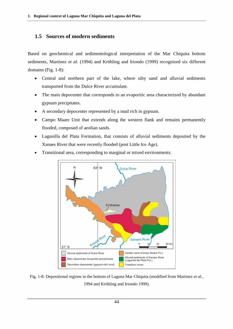
1. Regional context of Laguna Mar Chiquita and Laguna del Plata
44
1.5 Sources of modern sediments
Based on geochemical and sedimentological interpretation of the Mar Chiquita bottom
sediments, Martínez et al. (1994) and Kröhling and Iriondo (1999) recognized six different
domains (Fig. 1-8):
Central and northern part of the lake, where silty sand and alluvial sediments
transported from the Dulce River accumulate.
The main depocenter that corresponds to an evaporitic area characterized by abundant
gypsum precipitates.
A secondary depocenter represented by a mud rich in gypsum.
Campo Maare Unit that extends along the western flank and remains permanently
flooded, composed of aeolian sands.
Lagunilla del Plata Formation, that consists of alluvial sediments deposited by the
Xanaes River that were recently flooded (post Little Ice Age).
Transitional area, corresponding to marginal or mixed environments.
Fig. 1-8: Depositional regions in the bottom of Laguna Mar Chiquita (modified from Martinez et al.,
1994 and Kröhling and Iriondo 1999).
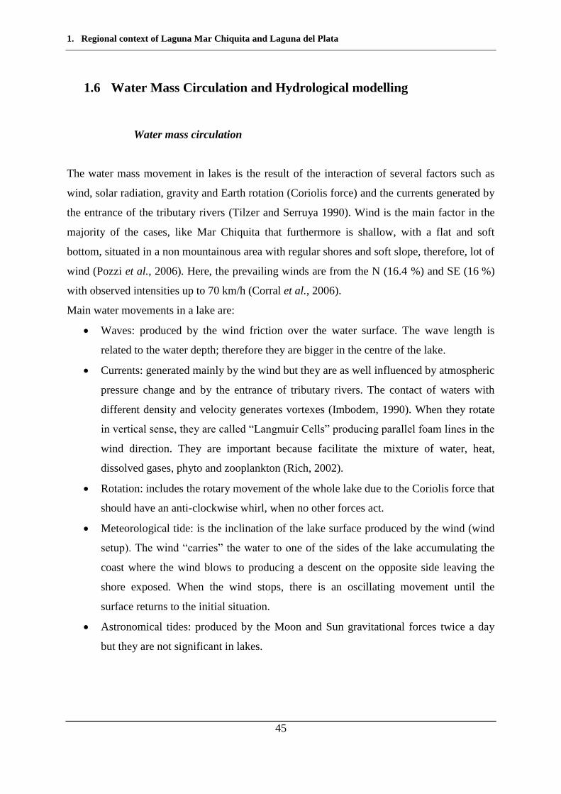
1. Regional context of Laguna Mar Chiquita and Laguna del Plata
45
1.6 Water Mass Circulation and Hydrological modelling
Water mass circulation
The water mass movement in lakes is the result of the interaction of several factors such as
wind, solar radiation, gravity and Earth rotation (Coriolis force) and the currents generated by
the entrance of the tributary rivers (Tilzer and Serruya 1990). Wind is the main factor in the
majority of the cases, like Mar Chiquita that furthermore is shallow, with a flat and soft
bottom, situated in a non mountainous area with regular shores and soft slope, therefore, lot of
wind (Pozzi et al., 2006). Here, the prevailing winds are from the N (16.4 %) and SE (16 %)
with observed intensities up to 70 km/h (Corral et al., 2006).
Main water movements in a lake are:
Waves: produced by the wind friction over the water surface. The wave length is
related to the water depth; therefore they are bigger in the centre of the lake.
Currents: generated mainly by the wind but they are as well influenced by atmospheric
pressure change and by the entrance of tributary rivers. The contact of waters with
different density and velocity generates vortexes (Imbodem, 1990). When they rotate
in vertical sense, they are called “Langmuir Cells” producing parallel foam lines in the
wind direction. They are important because facilitate the mixture of water, heat,
dissolved gases, phyto and zooplankton (Rich, 2002).
Rotation: includes the rotary movement of the whole lake due to the Coriolis force that
should have an anti-clockwise whirl, when no other forces act.
Meteorological tide: is the inclination of the lake surface produced by the wind (wind
setup). The wind “carries” the water to one of the sides of the lake accumulating the
coast where the wind blows to producing a descent on the opposite side leaving the
shore exposed. When the wind stops, there is an oscillating movement until the
surface returns to the initial situation.
Astronomical tides: produced by the Moon and Sun gravitational forces twice a day
but they are not significant in lakes.
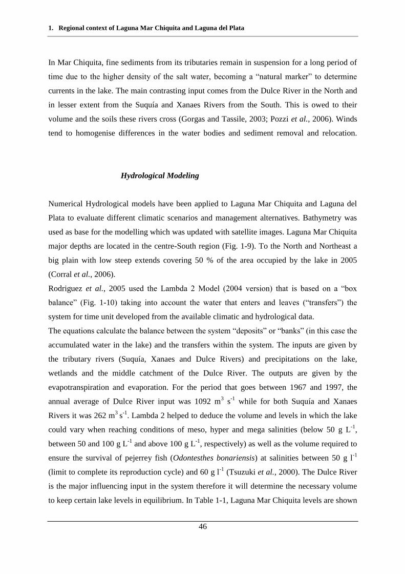
1. Regional context of Laguna Mar Chiquita and Laguna del Plata
46
In Mar Chiquita, fine sediments from its tributaries remain in suspension for a long period of
time due to the higher density of the salt water, becoming a “natural marker” to determine
currents in the lake. The main contrasting input comes from the Dulce River in the North and
in lesser extent from the Suquía and Xanaes Rivers from the South. This is owed to their
volume and the soils these rivers cross (Gorgas and Tassile, 2003; Pozzi et al., 2006). Winds
tend to homogenise differences in the water bodies and sediment removal and relocation.
Hydrological Modeling
Numerical Hydrological models have been applied to Laguna Mar Chiquita and Laguna del
Plata to evaluate different climatic scenarios and management alternatives. Bathymetry was
used as base for the modelling which was updated with satellite images. Laguna Mar Chiquita
major depths are located in the centre-South region (Fig. 1-9). To the North and Northeast a
big plain with low steep extends covering 50 % of the area occupied by the lake in 2005
(Corral et al., 2006).
Rodriguez et al., 2005 used the Lambda 2 Model (2004 version) that is based on a “box
balance” (Fig. 1-10) taking into account the water that enters and leaves (“transfers”) the
system for time unit developed from the available climatic and hydrological data.
The equations calculate the balance between the system “deposits” or “banks” (in this case the
accumulated water in the lake) and the transfers within the system. The inputs are given by
the tributary rivers (Suquía, Xanaes and Dulce Rivers) and precipitations on the lake,
wetlands and the middle catchment of the Dulce River. The outputs are given by the
evapotranspiration and evaporation. For the period that goes between 1967 and 1997, the
annual average of Dulce River input was 1092 m3 s-1 while for both Suquía and Xanaes
Rivers it was 262 m3 s-1. Lambda 2 helped to deduce the volume and levels in which the lake
could vary when reaching conditions of meso, hyper and mega salinities (below 50 g L-1,
between 50 and 100 g L-1 and above 100 g L-1, respectively) as well as the volume required to
ensure the survival of pejerrey fish (Odontesthes bonariensis) at salinities between 50 g l-1
(limit to complete its reproduction cycle) and 60 g l-1 (Tsuzuki et al., 2000). The Dulce River
is the major influencing input in the system therefore it will determine the necessary volume
to keep certain lake levels in equilibrium. In Table 1-1, Laguna Mar Chiquita levels are shown
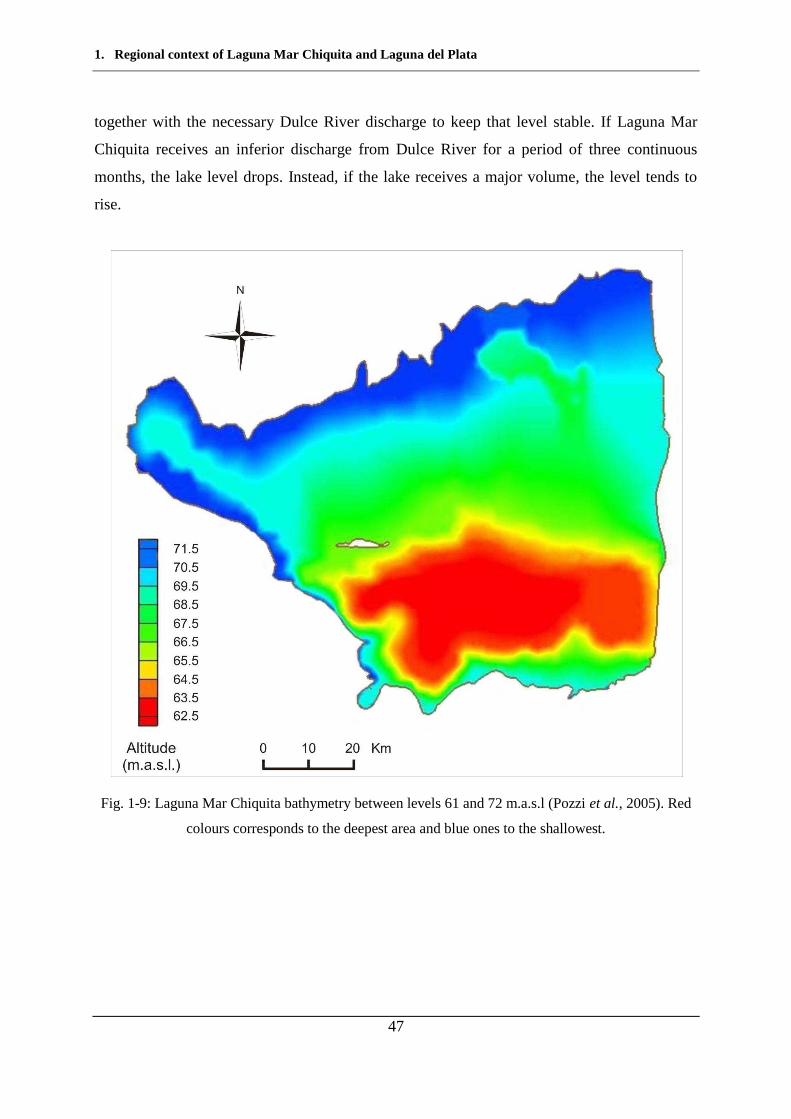
1. Regional context of Laguna Mar Chiquita and Laguna del Plata
47
together with the necessary Dulce River discharge to keep that level stable. If Laguna Mar
Chiquita receives an inferior discharge from Dulce River for a period of three continuous
months, the lake level drops. Instead, if the lake receives a major volume, the level tends to
rise.
Fig. 1-9: Laguna Mar Chiquita bathymetry between levels 61 and 72 m.a.s.l (Pozzi et al., 2005). Red
colours corresponds to the deepest area and blue ones to the shallowest.
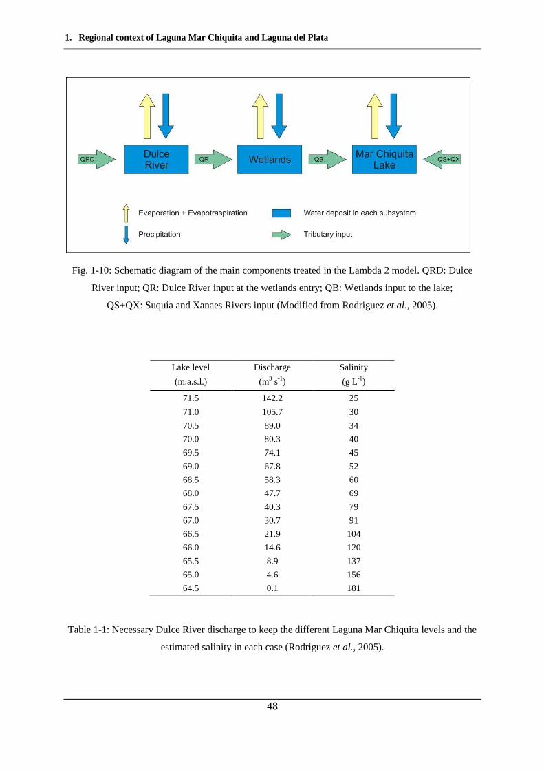
1. Regional context of Laguna Mar Chiquita and Laguna del Plata
48
Fig. 1-10: Schematic diagram of the main components treated in the Lambda 2 model. QRD: Dulce
River input; QR: Dulce River input at the wetlands entry; QB: Wetlands input to the lake;
QS+QX: Suquía and Xanaes Rivers input (Modified from Rodriguez et al., 2005).
Lake level Discharge Salinity
(m.a.s.l.) (m3 s-1) (g L-1)
71.5 142.2 25
71.0 105.7 30
70.5 89.0 34
70.0 80.3 40
69.5 74.1 45
69.0 67.8 52
68.5 58.3 60
68.0 47.7 69
67.5 40.3 79
67.0 30.7 91
66.5 21.9 104
66.0 14.6 120
65.5 8.9 137
65.0 4.6 156
64.5 0.1 181
Table 1-1: Necessary Dulce River discharge to keep the different Laguna Mar Chiquita levels and the
estimated salinity in each case (Rodriguez et al., 2005).
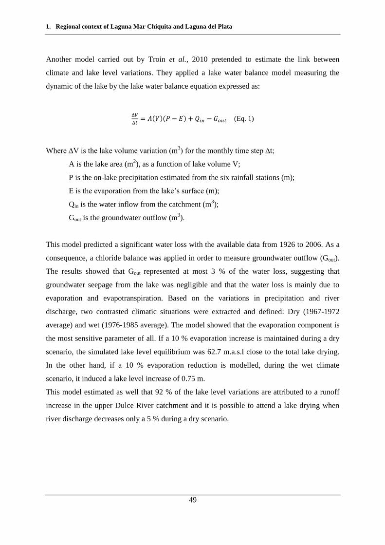
1. Regional context of Laguna Mar Chiquita and Laguna del Plata
49
Another model carried out by Troin et al., 2010 pretended to estimate the link between
climate and lake level variations. They applied a lake water balance model measuring the
dynamic of the lake by the lake water balance equation expressed as:
(Eq. 1)
Where ∆V is the lake volume variation (m3) for the monthly time step ∆t;
A is the lake area (m2), as a function of lake volume V;
P is the on-lake precipitation estimated from the six rainfall stations (m);
E is the evaporation from the lake’s surface (m);
Qin is the water inflow from the catchment (m3);
Gout is the groundwater outflow (m3).
This model predicted a significant water loss with the available data from 1926 to 2006. As a
consequence, a chloride balance was applied in order to measure groundwater outflow (Gout).
The results showed that Gout represented at most 3 % of the water loss, suggesting that
groundwater seepage from the lake was negligible and that the water loss is mainly due to
evaporation and evapotranspiration. Based on the variations in precipitation and river
discharge, two contrasted climatic situations were extracted and defined: Dry (1967-1972
average) and wet (1976-1985 average). The model showed that the evaporation component is
the most sensitive parameter of all. If a 10 % evaporation increase is maintained during a dry
scenario, the simulated lake level equilibrium was 62.7 m.a.s.l close to the total lake drying.
In the other hand, if a 10 % evaporation reduction is modelled, during the wet climate
scenario, it induced a lake level increase of 0.75 m.
This model estimated as well that 92 % of the lake level variations are attributed to a runoff
increase in the upper Dulce River catchment and it is possible to attend a lake drying when
river discharge decreases only a 5 % during a dry scenario.
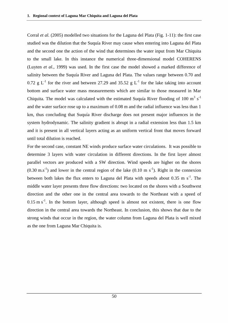
1. Regional context of Laguna Mar Chiquita and Laguna del Plata
50
Corral et al. (2005) modelled two situations for the Laguna del Plata (Fig. 1-11): the first case
studied was the dilution that the Suquía River may cause when entering into Laguna del Plata
and the second one the action of the wind that determines the water input from Mar Chiquita
to the small lake. In this instance the numerical three-dimensional model COHERENS
(Luyten et al., 1999) was used. In the first case the model showed a marked difference of
salinity between the Suquía River and Laguna del Plata. The values range between 0.70 and
0.72 g L-1 for the river and between 27.29 and 35.52 g L-1 for the lake taking into account
bottom and surface water mass measurements which are similar to those measured in Mar
Chiquita. The model was calculated with the estimated Suquía River flooding of 100 m3 s-1
and the water surface rose up to a maximum of 0.08 m and the radial influence was less than 1
km, thus concluding that Suquía River discharge does not present major influences in the
system hydrodynamic. The salinity gradient is abrupt in a radial extension less than 1.5 km
and it is present in all vertical layers acting as an uniform vertical front that moves forward
until total dilution is reached.
For the second case, constant NE winds produce surface water circulations. It was possible to
determine 3 layers with water circulation in different directions. In the first layer almost
parallel vectors are produced with a SW direction. Wind speeds are higher on the shores
(0.30 m.s-1) and lower in the central region of the lake (0.10 m s-1). Right in the connexion
between both lakes the flux enters to Laguna del Plata with speeds about 0.35 m s-1. The
middle water layer presents three flow directions: two located on the shores with a Southwest
direction and the other one in the central area towards to the Northeast with a speed of
0.15 m s-1. In the bottom layer, although speed is almost not existent, there is one flow
direction in the central area towards the Northeast. In conclusion, this shows that due to the
strong winds that occur in the region, the water column from Laguna del Plata is well mixed
as the one from Laguna Mar Chiquita is.
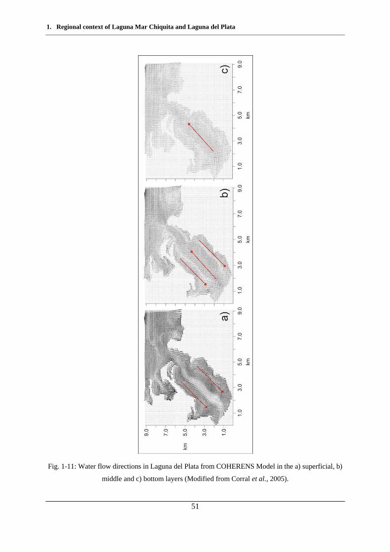
1. Regional context of Laguna Mar Chiquita and Laguna del Plata
51
Fig. 1-11: Water flow directions in Laguna del Plata from COHERENS Model in the a) superficial, b)
middle and c) bottom layers (Modified from Corral et al., 2005).
1. Regional context of Laguna Mar Chiquita and Laguna del Plata
52
1.7 Paleolimnology
Recent studies allowed to reconstruct the environmental fluctuations from the late Pleistocene
(last 14000 year) using the sedimentological record of different short cores taken at Laguna
Mar Chiquita and Laguna del Plata (Piovano et al., 2006). As it was mentioned before, Mar
Chiquita has suffered changes in its size due to the variable water inputs from its main
tributaries which respond to increasing and decreasing average regional precipitation. High or
low lake levels were defined whether they are over or below the altitude of 66.5 m.a.s.l.
(Piovano et al., 2002). High salinity values were measured during the low level periods that
occurred in the 20th Century: 360 g L-1 in 1911 (Frank, 1915), 251 g L-1 in 1951 (Bertoldi de
Pomar, 1953) and 270 g L-1 in 1970 (Martinez, 1991). This intense deficit in the water budget
is attributed to the strongly negative hydrological balance that affected central Argentina
during the first 70 years of the 20th Century (Piovano et al., 2009; Troin et al., 2010). An
onset of higher regional precipitations started early in the 1970s and the Laguna Mar Chiquita
lake level started to rise generating the connection of this lake with Laguna del Plata that
persist nowadays (Piovano et al., 2002; 2004a,b). In 1986 Martinez (1991) measured salinities
of 29 g L-1 and three years later this value rose to 35 g L-1 in coincidence with a 1.3 m water
depth decrease. He also compared the compositional relationships founding that they
reminded the same for the major ions (Na, Cl and SO4-2). Mar Chiquita waters are classified
as of the Na-Cl- SO4-2 type.
Using 210Pb dating, Piovano et al. (2002, 2006) determined sediment ages in two cores taken
from Laguna Mar Chiquita (TMC-5 and TMC-14; Fig. 1-12).The determination of sediment
ages along with the description of the sedimentological characteristics and the analysis of
meteorological data, allowed a reconstruction of the hydrological history of the lake.
Sediments accumulated during the 20th Century correspond to the first 50 cm of the core.
High lake levels were recognized from 1977 to present, while a period of low lake levels
extended from 1968 to 1972. During the high level phase, the sedimentation rate in Laguna
Mar Chiquita varied between 0.77 and 1.12 cm y-1, while during low lake-levels values were
between 0.25 to 0.34 cm y-1. The average sedimentation rate (ASR) was calculated through a
linear regression along the treated section (54 cm) resulting in 0.41 and 0.49 cm y-1. Older
ages below 54 cm were obtained using the mean ASR value and assuming constant rates.
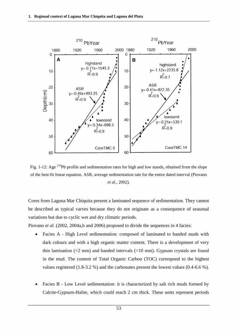
1. Regional context of Laguna Mar Chiquita and Laguna del Plata
53
Fig. 1-12: Age 210Pb profile and sedimentation rates for high and low stands, obtained from the slope
of the best-fit linear equation. ASR, average sedimentation rate for the entire dated interval (Piovano
et al., 2002).
Cores from Laguna Mar Chiquita present a laminated sequence of sedimentation. They cannot
be described as typical varves because they do not originate as a consequence of seasonal
variations but due to cyclic wet and dry climatic periods.
Piovano et al. (2002, 2004a,b and 2006) proposed to divide the sequences in 4 facies:
Facies A - High Level sedimentation: composed of laminated to banded muds with
dark colours and with a high organic matter content. There is a development of very
thin lamination (<2 mm) and banded intervals (<10 mm). Gypsum crystals are found
in the mud. The content of Total Organic Carbon (TOC) correspond to the highest
values registered (1.8-3.2 %) and the carbonates present the lowest values (0.4-6.6 %).
Facies B - Low Level sedimentation: it is characterized by salt rich muds formed by
Calcite-Gypsum-Halite, which could reach 2 cm thick. These units represent periods
1. Regional context of Laguna Mar Chiquita and Laguna del Plata
54
of very low lake levels and high salinities. They contain high carbonate concentrations
(25 %) and low TOC (0.5-1.6 %).
Facies C – Intermediate Level sedimentation: it presents intermediate characteristics
compared to the previous two facies of high and low levels. They are laminated to
banded muds with intermediate contents of TOC and carbonates. It is possible to find
these units between the very salt rich levels and the organic matter rich ones. TOC
ranges between 1.3 and 2.4 % and carbonates between 5.6 and 13.3 %.
Facies D – Short Pulses of Intermediate Level sedimentation: they are organic matter
rich muds with very thin calcite laminas. They present up to 2.1 % of TOC, gypsum
crystals. They were sedimented when the lake level was intermediate and last for a
short period.
Energy, nutrients and evaporitic mineral precipitation fluxes are controlled by the variation in
salinity associated to the lake level changes (Martínez 1991; Reati et al., 1997) resulting in
organic matter rich facies in high levels and evaporitic rich facies during low levels. The
abundant clastic fraction present in the sediments shows that during the positive water
balances, the fluvial input is significant (Piovano et al., 2006).
Some studies concerning the isotopic record in Mar Chiquita were done by Dapeña et al.
(1997), Dapeña and Panarello (2001) and Piovano et al. (2004a, 2006). The shallowness of
Mar Chiquita and the well mixed state of its waters allows to perform an isotopic balance
(Reati et al., 1997; Dapeña and Panarello 2001). Piovano et al. (2004b, 2006), carried out
some analysis concerning carbon, carbonate and oxygen isotope analysis. Analyses of 18Ocarb
and 13Ccarb showed that facies A contains the most negative values (-3.1 ‰ and between -5.3
and -2.1 ‰ respectively). In the other hand, facies B and D show the less negative values
(18Ocarb = 0.8 ‰; 13Ccarb = -1.3 ‰ and 18Ocarb = 1.7 ‰; 13Ccarb = -0.5‰ respectively) while
facies C presents intermediate isotopes values (18Ocarb = -1.0 ‰ and 13Ccarb = -2.5 ‰).
1. Regional context of Laguna Mar Chiquita and Laguna del Plata
55
Therefore, a model representing the lake level fluctuations and the associated sedimentary
record was performed. Sediments reflect their precipitation from waters with different
isotopic compositions which is the consequence of varying P-E (Precipitation – Evaporation)
ratios (Fig. 1-13, Piovano et al., 2002, 2004a,b, 2006):
- Facies like A were characterised by periods where P>E with lower salinities (28-60 g L-1)
and high organic matter level due to a high biological activity are registered for example
between 1997-2005.
- Facies C and D are represented by P=E with intermediate salinities (80 g L-1) indicating an
evolution in the system, progressing water dilution as consequence of fresh water input,
increasing levels of organic matter accumulation and a diminution on the carbonates
precipitation, the period between 1972 and 1977 is an example of this situation.
- Facies like B are given when P<E, characterized by a negative water balance with high
salinities (360 g L-1), low water levels, high carbonates accumulation rate, development of
evaporitic levels (Piovano et al., 2006) and diminution of the biological activity with a
decrease in the organic matter accumulation (Reati et al., 1997). Periods like this were
registered in 1911 (Frank, 1915). The isotopic study helped to confirm that the water losses
are only due to evaporation discarding the groundwater leaking (Dapeña and Panarello, 2001).
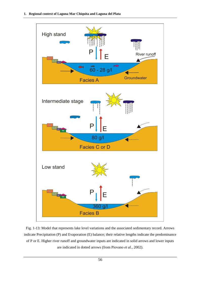
1. Regional context of Laguna Mar Chiquita and Laguna del Plata
56
Fig. 1-13: Model that represents lake level variations and the associated sedimentary record. Arrows
indicate Precipitation (P) and Evaporation (E) balance; their relative lengths indicate the predominance
of P or E. Higher river runoff and groundwater inputs are indicated in solid arrows and lower inputs
are indicated in dotted arrows (from Piovano et al., 2002).
2. Hazardous elements in the environment: Mercury and Arsenic
57
2. Hazardous elements in the
environment: Mercury and Arsenic
2. Hazardous elements in the environment: Mercury and Arsenic
58
2. Hazardous elements in the environment: Mercury and Arsenic
59
Elements that occur in the Earth’s crust in amounts less than 0.1 % (1000 mg kg-1) are known
as “trace metals”. Many elements are present as trace amounts in living matter. Some of these
elements are essential for the growth, development and health of organisms, but the
quantitative difference between essential amounts and biological excess (therefore hazardous)
is very small (Kabata-Pendias, 2010). In this study the distribution and geochemistry of
mercury (Hg) and arsenic (As) is presented for the Suquía River basin and the saline lake of
Laguna del Plata. Hg has been widely studied as a global flux indicator especially in the
Northern Hemisphere (e.g., Fitzgerald and Mason, 1997; Fitzgerald et al., 1998; Fitzgerald
and Lamborg, 2003) but in the Southern Hemisphere and notably Argentina studies are
scarce. In this context, the study of Hg accumulation in the sedimentary record in Laguna del
Plata is a contribution to understand the fluxes of global Hg in a climatic-sensitive region of
southern South America (e.g. Piovano et al., 2004a,b). On the other hand, As has been widely
studied in the Chaco Pampean Region due to the high concentration of this element in
groundwater (that in most of the cases exceeds the recommended guideline value for drinking
water) and its strong association to the loess present in the region (e.g. Smedley and
Kinniburgh, 2002). But studies concerning fresh water and the relationship to saline systems
are rare.
2.1 Mercury
2.1.1 Mercury in the environment
Mercury is a chemical element with the particularity to be the only common metal liquid at
ordinary temperatures, rarely occurs free in nature. The main ore is cinnabar (HgS – Fig. 2-1),
when it is heated in a current air and by condensing the vapour it is possible to obtain the
metal. Mercury is widely used in laboratory work for making thermometers, barometers,
diffusion pumps, and many other instruments, as well as in making pesticides, mercury cells
for caustic soda and chlorine production, dental preparations, antifouling paint, batteries, and
catalysts (Hammond, 2005).
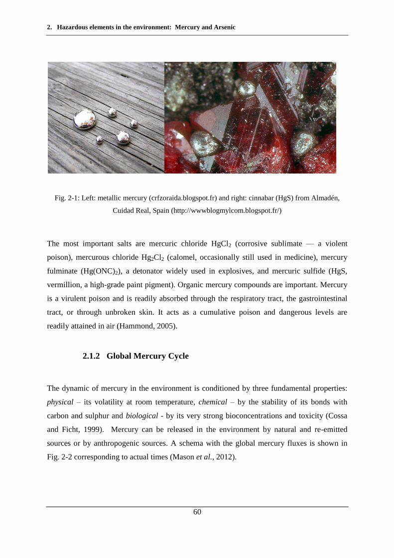
2. Hazardous elements in the environment: Mercury and Arsenic
60
Fig. 2-1: Left: metallic mercury (crfzoraida.blogspot.fr) and right: cinnabar (HgS) from Almadén,
Cuidad Real, Spain (http://wwwblogmylcom.blogspot.fr/)
The most important salts are mercuric chloride HgCl2 (corrosive sublimate — a violent
poison), mercurous chloride Hg2Cl2 (calomel, occasionally still used in medicine), mercury
fulminate (Hg(ONC)2), a detonator widely used in explosives, and mercuric sulfide (HgS,
vermillion, a high-grade paint pigment). Organic mercury compounds are important. Mercury
is a virulent poison and is readily absorbed through the respiratory tract, the gastrointestinal
tract, or through unbroken skin. It acts as a cumulative poison and dangerous levels are
readily attained in air (Hammond, 2005).
2.1.2 Global Mercury Cycle
The dynamic of mercury in the environment is conditioned by three fundamental properties:
physical – its volatility at room temperature, chemical – by the stability of its bonds with
carbon and sulphur and biological - by its very strong bioconcentrations and toxicity (Cossa
and Ficht, 1999). Mercury can be released in the environment by natural and re-emitted
sources or by anthropogenic sources. A schema with the global mercury fluxes is shown in
Fig. 2-2 corresponding to actual times (Mason et al., 2012).
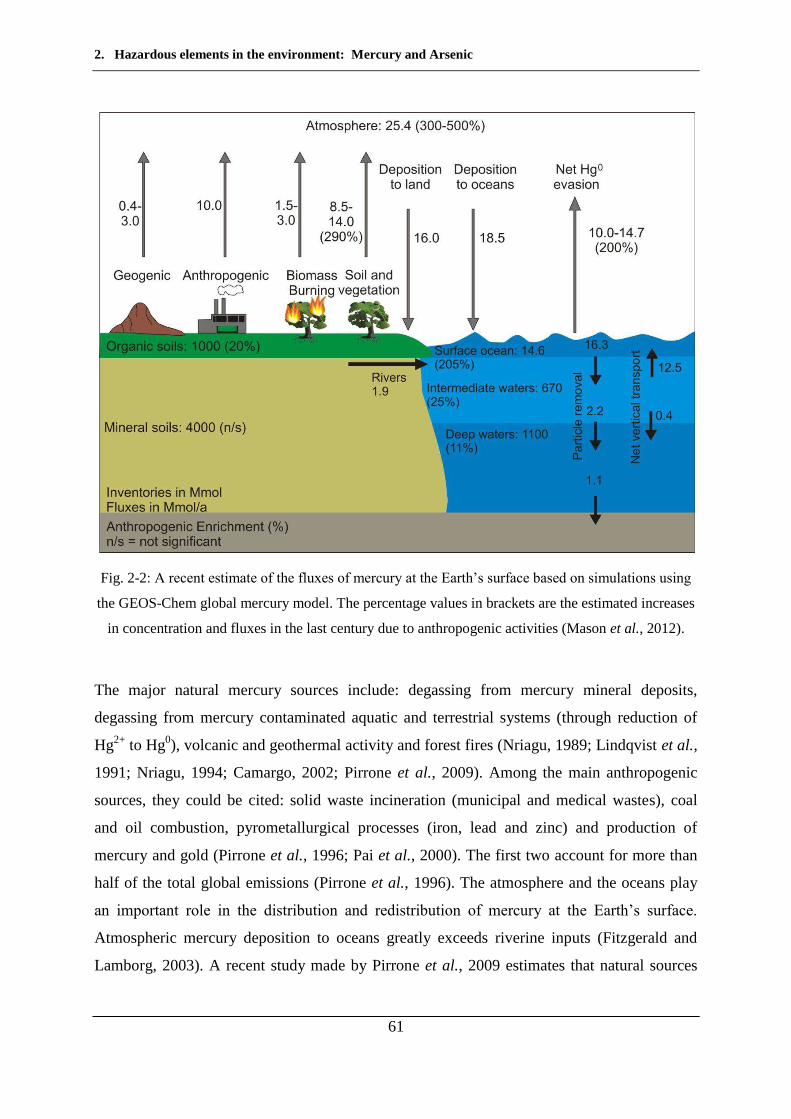
2. Hazardous elements in the environment: Mercury and Arsenic
61
Fig. 2-2: A recent estimate of the fluxes of mercury at the Earth’s surface based on simulations using
the GEOS-Chem global mercury model. The percentage values in brackets are the estimated increases
in concentration and fluxes in the last century due to anthropogenic activities (Mason et al., 2012).
The major natural mercury sources include: degassing from mercury mineral deposits,
degassing from mercury contaminated aquatic and terrestrial systems (through reduction of
Hg2+ to Hg0), volcanic and geothermal activity and forest fires (Nriagu, 1989; Lindqvist et al.,
1991; Nriagu, 1994; Camargo, 2002; Pirrone et al., 2009). Among the main anthropogenic
sources, they could be cited: solid waste incineration (municipal and medical wastes), coal
and oil combustion, pyrometallurgical processes (iron, lead and zinc) and production of
mercury and gold (Pirrone et al., 1996; Pai et al., 2000). The first two account for more than
half of the total global emissions (Pirrone et al., 1996). The atmosphere and the oceans play
an important role in the distribution and redistribution of mercury at the Earth’s surface.
Atmospheric mercury deposition to oceans greatly exceeds riverine inputs (Fitzgerald and
Lamborg, 2003). A recent study made by Pirrone et al., 2009 estimates that natural sources
2. Hazardous elements in the environment: Mercury and Arsenic
62
release about 5.21x10³ tons of mercury per year, part of which represent previously deposited
anthropogenic and natural mercury from the atmosphere to ecosystem-receptors due to
historic releases and part is a new contribution from natural reservoirs. Current anthropogenic
sources, which include a large number of industrial point sources, are estimated to release
about 2.91 x10³ tons of mercury on an annual basis, being the fossil fuel-fired power plants
(1.42x10³ t y-1) the major contributor. Between natural and anthropogenic emissions they
estimate that nearly 8.12x10³ tons of mercury are released annually to the global atmosphere.
It has been estimated by several authors that current atmospheric deposition is 3 (Von Gunten
et al., 1997, Johannessen et al., 2005), 4 (Fitzgerald et al., 1998; Heyvaert et al., 2000;
Bindler, 2003), 10 (Bindler, 2003), 16 (Liu et al., 2012) and even 24 times (Heyvaert et al.,
2000) higher than pre-industrial flux.
2.1.2.1 Mercury speciation
The speciation of Hg regulates toxicity, transport pathways and residence time within the
different compartments of the ecosystem (Lindqvist et al., 1991).
The atmospheric mercury is mainly made up of gaseous Hg (about 95 to 100 %) and the
remainder is associated with particles (Lindqvist et al., 1991). The chemical forms of Hg in
the atmosphere are still under discussion (Lindqvist et al., 1991; Cossa and Ficht, 1999) but
the total predominance of elemental Hg is generally accepted. Besides elemental Hg,
methylmercury (MeHg) is present in air but only in minor quantities ~0 to 5 % (Bloom and
Fitzgerald, 1988) which increase with altitude (Lindqvist et al., 1991).
In natural waters Hg is often fractionated by their different ability to be reduced to elemental
Hg (Lindqvist et al., 1991). Mercury speciation in natural waters has evolved thanks to clean
laboratory protocols (Gill and Fitzgerald, 1985; Fitzgerald, 1989) and analytical studies
(Bloom and Fitzgerald, 1988; Bloom, 1989). Reactive Hg (HgR) consists of Hg species that
are readily reduced by SnC12 under acidic conditions. This fraction is comprised primarily of
labile inorganic and organic complexes of Hg(II), and of labile particulate associations. Total
Hg (HgT) is a measure of the total dissolved and particulate Hg in an unfiltered sample. In dry
and wet precipitation, a large part of the HgR content is associated with particles (Ferrara et
2. Hazardous elements in the environment: Mercury and Arsenic
63
al., 1986; Ahmed et al., 1987; Iverfeldt and Rodhe, 1988) and colloid particles (Brosset and
Lord, 1991) and as in the air MeHg species are also present (Ahmed et al., 1987; Lee, 1987;
Bloom and Watras, 1989). Precipitations falling through a tree canopy can lead in interactions
between Hg and dissolved organic complexes (DOC). The type and amount of compounds
associated to canopy will vary to those found in the wet deposition of an open field. The
canopy may also act as a sink of Hg in rain due to binding in fixed organic matter and thus,
affecting the type and level of Hg species reaching the ground (Lindqvist et al., 1991).
In lake waters, Hg is associated to particles as well with DOC, and the levels of the fractions
may vary with seasonal variation. Most of the MeHg is probably associated to DOC. Little is
known about the type of complexation between MeHg and other Hg compounds with DOC in
water, since DOC is a heterogeneous mixture consisting mainly of fulvic and humic acids
(50 to 80 %), carbohydrates, carboxylic acids, amino acids and hydrocarbons. These are
capable of forming complexes with many metal ions as a result of the ligand groups present
(-COOH, -OH, -NH2 and –RSH) (Lindqvist et al., 1991).
Low but detectable concentrations of dissolved gaseous Hg are usually present in all types of
freshwater systems. It is likely that elemental Hg constitutes most of the dissolved gaseous Hg
in lakes (Bloom and Watras, 1989; Fitzgerald et al., 1990; Lindqvist et al., 1991) and the
evasion of elemental mercury (Hg0) at the water surface is an important natural flux of Hg to
the atmosphere (Vandal et al., 1991).
Concerning sea water, dissolved gaseous Hg concentrations have been found at supersaturated
levels in the equatorial region (Kim and Fitzgerald, 1986). The dissolved gaseous Hg consists
mainly of elemental Hg, but in sub-surface water also to some degree of dimethyl mercury
(DMHg). However, Hg is predominantly ( 80 %) in the reactive form in open ocean waters
(Gill and Fitzgerald, 1987; Cossa and Noel, 1987).
Hg concentrations in the raw humus layer and the regional variation can be assumed to reflect
mainly the atmospheric deposition pattern, integrated over decades or even centuries. Some
Hg in the litter has, however, probably also been taken up by the roots and gaseous Hg may
have been brought to the surface layer by diffusion from below and, by biological activity,
some mineral matter from below may have been mixed into the organic layer. Therefore, to
some extent the Hg concentration of raw humus and the regional distribution pattern will also
be influenced by the Hg content in parent material and bedrock (Lindqvist et al., 1991).
2. Hazardous elements in the environment: Mercury and Arsenic
64
2.1.3 Dynamics of Hg
2.1.3.1 Redox reactions in the atmosphere
Oceans and coastal seas release Hg to the atmosphere especially in the form of elemental Hg
(Hg0) and some traces of DMHg ((CH3)2Hg0) coming from deep waters. MeHg ((CH3)2Hg+),
decomposed from DMHg, constitutes less than 1 % of Hg in the rain (Cossa and Fitch, 1999).
The average residence time could go from hours for some oxidized Hg(II) species to a more
than one year for elemental Hg (Fitzgerald, 1989; Slemr, 1992; Cossa and Fitch, 1999;
Fitzgerald and Lamborg, 2003).
Many divalent Hg compounds exist as undissociated molecules in water solution as well as in
the gaseous phase. Such molecules that may occur in the atmosphere are HgC12, HgBr2,
Hg(OH)2, Hg(SH)2, Hg(CN)2, etc. (Lindqvist et al., 1991).
It is known that elemental Hg reacts with O3 (P’Yankov, 1949) but it does it as well with Cl2
(Hall, 1990) in the gas phase.
Some authors have shown that SO2(g) can reduce HgO at a very slow rate (Zacharewski et al.,
1987). Studies concerning photochemical reduction of dissolved divalent Hg were performed
in laboratory (Iverfeldt, 1984; Munthe and Linqvist, 1990) and on the field (Brosset, 1987).
They showed that Hg(SO3)22- is dissociated thermally while Hg(OH)2 is photodissociated.
This can occur because many Hg species (Fig. 2-3) such as complexes with OH-, HS-, C1- and
organic ligands can absorb radiation in the highly energetic UV range (270-400 nm) of the
solar spectrum (Fujita et al., 1973; Stromberg et al., 1991).
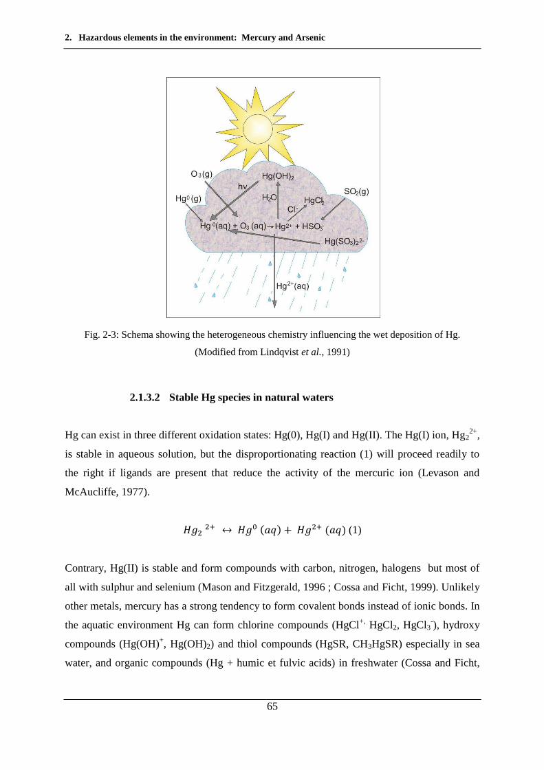
2. Hazardous elements in the environment: Mercury and Arsenic
65
Fig. 2-3: Schema showing the heterogeneous chemistry influencing the wet deposition of Hg.
(Modified from Lindqvist et al., 1991)
2.1.3.2 Stable Hg species in natural waters
Hg can exist in three different oxidation states: Hg(0), Hg(I) and Hg(II). The Hg(I) ion, Hg22+,
is stable in aqueous solution, but the disproportionating reaction (1) will proceed readily to
the right if ligands are present that reduce the activity of the mercuric ion (Levason and
McAucliffe, 1977).
(1)
Contrary, Hg(II) is stable and form compounds with carbon, nitrogen, halogens but most of
all with sulphur and selenium (Mason and Fitzgerald, 1996 ; Cossa and Ficht, 1999). Unlikely
other metals, mercury has a strong tendency to form covalent bonds instead of ionic bonds. In
the aquatic environment Hg can form chlorine compounds (HgCl+, HgCl2, HgCl3-), hydroxy
compounds (Hg(OH)+, Hg(OH)2) and thiol compounds (HgSR, CH3HgSR) especially in sea
water, and organic compounds (Hg + humic et fulvic acids) in freshwater (Cossa and Ficht,
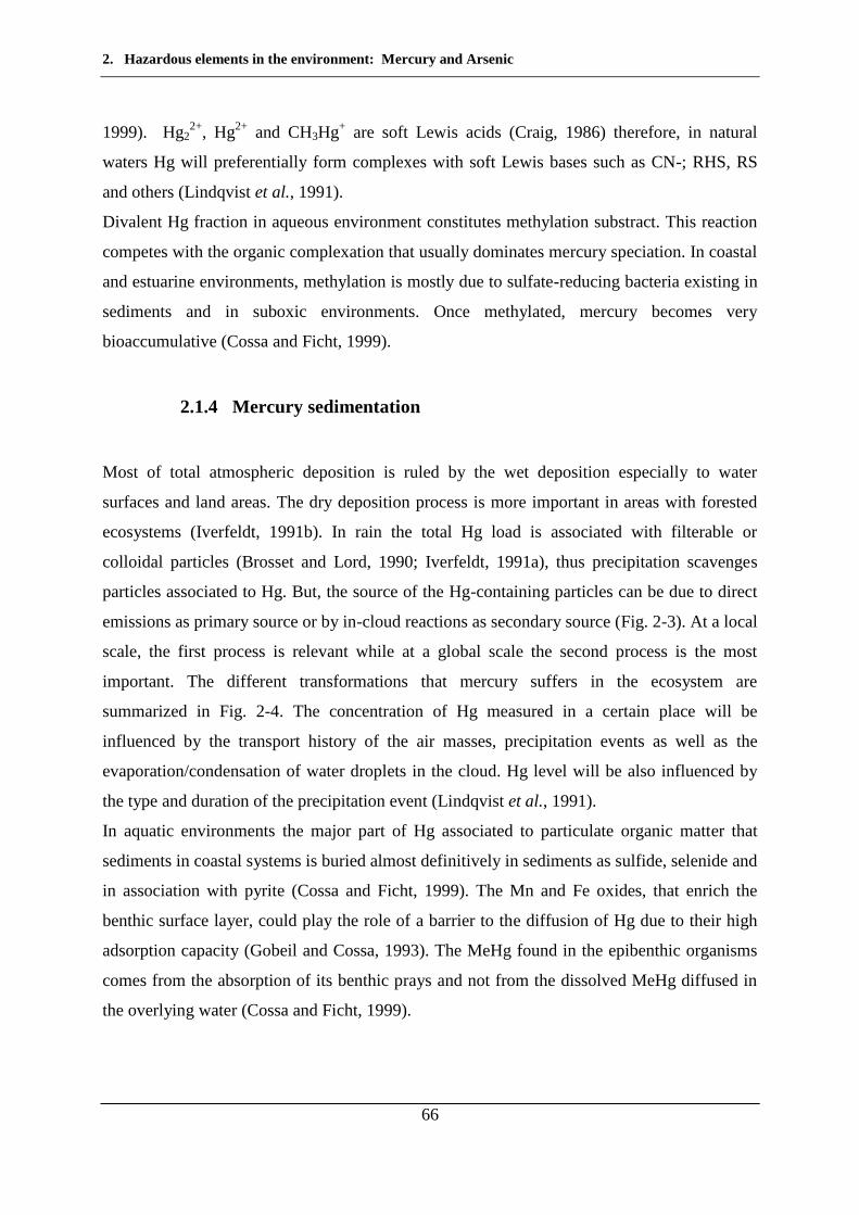
2. Hazardous elements in the environment: Mercury and Arsenic
66
1999). Hg22+, Hg2+ and CH3Hg+ are soft Lewis acids (Craig, 1986) therefore, in natural
waters Hg will preferentially form complexes with soft Lewis bases such as CN-; RHS, RS
and others (Lindqvist et al., 1991).
Divalent Hg fraction in aqueous environment constitutes methylation substract. This reaction
competes with the organic complexation that usually dominates mercury speciation. In coastal
and estuarine environments, methylation is mostly due to sulfate-reducing bacteria existing in
sediments and in suboxic environments. Once methylated, mercury becomes very
bioaccumulative (Cossa and Ficht, 1999).
2.1.4 Mercury sedimentation
Most of total atmospheric deposition is ruled by the wet deposition especially to water
surfaces and land areas. The dry deposition process is more important in areas with forested
ecosystems (Iverfeldt, 1991b). In rain the total Hg load is associated with filterable or
colloidal particles (Brosset and Lord, 1990; Iverfeldt, 1991a), thus precipitation scavenges
particles associated to Hg. But, the source of the Hg-containing particles can be due to direct
emissions as primary source or by in-cloud reactions as secondary source (Fig. 2-3). At a local
scale, the first process is relevant while at a global scale the second process is the most
important. The different transformations that mercury suffers in the ecosystem are
summarized in Fig. 2-4. The concentration of Hg measured in a certain place will be
influenced by the transport history of the air masses, precipitation events as well as the
evaporation/condensation of water droplets in the cloud. Hg level will be also influenced by
the type and duration of the precipitation event (Lindqvist et al., 1991).
In aquatic environments the major part of Hg associated to particulate organic matter that
sediments in coastal systems is buried almost definitively in sediments as sulfide, selenide and
in association with pyrite (Cossa and Ficht, 1999). The Mn and Fe oxides, that enrich the
benthic surface layer, could play the role of a barrier to the diffusion of Hg due to their high
adsorption capacity (Gobeil and Cossa, 1993). The MeHg found in the epibenthic organisms
comes from the absorption of its benthic prays and not from the dissolved MeHg diffused in
the overlying water (Cossa and Ficht, 1999).
2. Hazardous elements in the environment: Mercury and Arsenic
67
Fig. 2-4: Cycle of Hg. Reactions, transformations and transfers (hum = humic acid; SR-b = sulfate-
reducing bacteria; FeR = iron-reducing bacteria). Modified from Castelle, 2008.
2. Hazardous elements in the environment: Mercury and Arsenic
68
2.1.5 Mercury in the world and Argentina
The high mercury concentrations in countries such as Canada, France, Switzerland and China
observed at the beginning of the 19th Century were concomitant with the industrial and
demographic growth. The periods with the highest concentrations usually coincide with some
of the historical times with a marked industrial development such as the “golden age” in 1860,
the Second World War (1939-1945), development of uncontrolled mining activities in France
and some industrial spill accidents as it is the case in Canada late 1960s. These events were
the responsible of liberation and accumulation of large concentrations of this metal in
sediments. From half of the 20th Century to nowadays the aim is to reduce the mercury
concentrations released to the atmosphere applying clean technologies, amelioration on used
and waste waters and the implementation of more severe environmental laws (Von Gunten et
al., 1997; Johannessen et al., 2005; Castelle et al., 2007; Liu et al., 2012).
Estimations made by Pirrone et al. (1996) and Pacyna et al. (2003, 2006) for the years 1990-
1992, 1995 and 2000 respectively, indicate that North America and Europe have reduced its
global anthropogenic emissions to the atmosphere to less than 20 %. On the other hand, Asia
and Africa increased from less than 50 % to about 70 % of global emissions in ten years; this
increase is due to the fast economic development. Around 36 % of the total global emissions
correspond to anthropogenic sources and the major source corresponds to the combustion of
fossil fuels that vary between 15 and 18 % in Europe, North America and Asia (Pirrone et al.,
2009).
In the Southern Hemisphere, mercury concentrations are associated mainly to gold mining. In
countries such as Brazil, Colombia, Bolivia, Peru, French Guyana, among others, high Hg
levels were found in river and lake sediments, soils, fishes and human hairs in towns near the
mining areas. Hg is used for separation of gold particles through amalgamation. During this
process, a good amount of metallic Hg is also lost to rivers and soils through handling under
rough field conditions and to volatilization. After amalgamation, the Au-Hg complex is
burned in retorts but in most areas, this operation is done in open air, releasing Hg vapour to
the atmosphere. Furthermore, Hg rich tailings are left in most mining sites (Diaz, 2000;
Lacerda et al., 2004). In Brazil the gold mining boom was developed from 1979 to 1995 but
even nowadays high mercury levels are detected. This is due to the remobilization of
sediments and changes in land use such as conversion of forests to pasture (Olivero et al.,
2002; Rodrigues Bastos et al., 2006; Huguet et al., 2010). Sediments from de la Plata River in
2. Hazardous elements in the environment: Mercury and Arsenic
69
the Uruguayan coast were analyzed showing high concentrations of Hg and other heavy
metals that are related to municipal effluents, industrial waste, oil refinery among others
(Muñiz et al., 2004).
In lakes Guanaco, LP and Stuart M. located in the austral Patagonia of Chile, mercury
accumulation seem to be fairly constant during the 19th Century and the variations in Hg
concentrations in the sediments of these lakes are driven by changes in local precipitation
rates as well as leaching of Hg organic complexes from the catchment soils (Hermanns and
Biester, 2013).
Argentina in particular, the occurrence of Hg in sediments accumulated in freshwater systems
are scarce (i.e., Amin et al., 1996; Hudson-Edwards et al., 2001; Ronco et al., 2001;
Marcovecchio et al., 2001; Ribeiro Guevara et al., 2002, 2004, 2005, 2009, 2010; Arribére et
al., 2003; De Marco et al., 2006; Botté et al., 2010). Most of these studies are concentrated in
the Patagonia region and in coastal areas of the Buenos Aires province. For example, three
estuarine systems on the shores of Buenos Aires were studied and total Hg concentrations in
sediments and biota were analyzed between 1980 and 2005. The presence of Hg is mainly of
anthropogenic origin due that in the region, ports, towns and several industries exist. The
results indicate that total Hg values decreased significantly (p<0.001) in the last 25 years
attributing this tendency to the improvement in the industry practices of the region (De Marco
et al., 2006). In the Argentina’s Patagonia, the historical record of Hg was analyzed in two
sedimentary cores retrieved from lakes Tonček and Moreno in the Nahuel Huapi National
Park (Ribeiro Guevara et al., 2005, 2010). These authors found that recent Hg concentrations
are around 2.5 times higher than those registered in pre-industrial times. However, high Hg
concentrations were also measured in sediments of pre-industrial times that could be related to
ancient extended fires and volcanic activity. It is well known that volcanoes represent a
potentially important natural source of mercury in the atmosphere (Nriagu and Becker, 2003)
and especially this region that is located in the Southern Volcanic Zone (SVZ) that extends
from 33 to 46°S (Stern, 2004; Kratzmann et al., 2010) and has shown some eruptive activity
in the last two decades (e.g. Matthews et al., 1997). Typical Hg concentrations in rocks, soils
and sediments around the world are listed in Table 2-1.
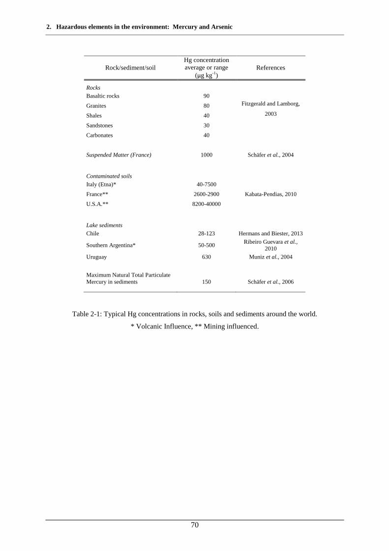
2. Hazardous elements in the environment: Mercury and Arsenic
70
Rock/sediment/soil
Hg concentration average or range
(µg kg-1) References
Rocks
Fitzgerald and Lamborg,
2003
Basaltic rocks 90
Granites 80
Shales 40
Sandstones 30
Carbonates 40
Suspended Matter (France) 1000 Schäfer et al., 2004
Contaminated soils
Italy (Etna)* 40-7500
Kabata-Pendias, 2010 France** 2600-2900
U.S.A.** 8200-40000
Lake sediments
Chile 28-123 Hermans and Biester, 2013
Southern Argentina* 50-500 Ribeiro Guevara et al.,
2010
Uruguay 630 Muniz et al., 2004
Maximum Natural Total Particulate Mercury in sediments
150 Schäfer et al., 2006
Table 2-1: Typical Hg concentrations in rocks, soils and sediments around the world.
* Volcanic Influence, ** Mining influenced.
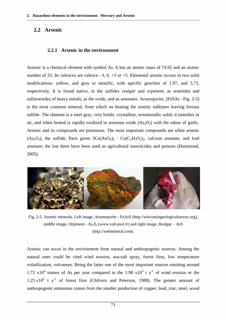
2. Hazardous elements in the environment: Mercury and Arsenic
71
2.2 Arsenic
2.2.1 Arsenic in the environment
Arsenic is a chemical element with symbol As. It has an atomic mass of 74.92 and an atomic
number of 33. Its valences are valence –3, 0, +3 or +5. Elemental arsenic occurs in two solid
modifications: yellow, and gray or metallic, with specific gravities of 1.97, and 5.73,
respectively. It is found native, in the sulfides realgar and orpiment, as arsenides and
sulfarsenides of heavy metals, as the oxide, and as arsenates. Arsenopyrite, (FeSAs –Fig. 2-5)
is the most common mineral, from which on heating the arsenic sublimes leaving ferrous
sulfide. The element is a steel gray, very brittle, crystalline, semimetallic solid; it tarnishes in
air, and when heated is rapidly oxidized to arsenous oxide (As2O3) with the odour of garlic.
Arsenic and its compounds are poisonous. The most important compounds are white arsenic
(As2O3), the sulfide, Paris green 3Cu(AsO2)2 · Cu(C2H3O2)2, calcium arsenate, and lead
arsenate; the last three have been used as agricultural insecticides and poisons (Hammond,
2005).
Fig. 2-5: Arsenic minerals. Left image, Arsenopyrite - FeAsS (http://wisconsingeologicalsurvey.org),
middle image, Orpiment - As2S3 (www.volcanol.fr) and right image, Realgar – AsS
(http://webmineral.com).
Arsenic can occur in the environment from natural and anthropogenic sources. Among the
natural ones could be cited wind erosion, sea-salt spray, forest fires, low temperature
volatilization, volcanoes. Being the latter one of the most important sources emitting around
1.72 x10⁴ tonnes of As per year compared to the 1.98 x10³ t y-1 of wind erosion or the
1.25 x10² t y-1 of forest fires (Chilvers and Peterson, 1988). The greater amount of
anthropogenic emissions comes from the smelter production of copper, lead, zinc, steel, wood
2. Hazardous elements in the environment: Mercury and Arsenic
72
fuel, clearance of land crops, arsenic chemical productions, waste incineration, generating in
total an estimate burden of 2.81 x10⁴ t y-1 of arsenic emissions to the atmosphere. These
authors estimate that 40 % of the atmospheric As emissions correspond to anthropogenic
inputs of which more than 40 % answer to copper smelting. In the other hand, 60 % of the
total atmospheric As emissions derive from natural sources with nearly 60 % of the total
natural flux coming from low temperature volatilization from soils and most of the remainder
from volcanoes.
2.2.2 Sources of Arsenic
2.2.2.1 Minerals
Arsenic is present in more than 200 minerals as major constituent. The range goes from
elemental As, arsenides, sulphides, oxides, arsenates As(V) and arsenites As(III) but the
greatest concentrations occur in mineralised ores associated to Cd, Pb, Ag, Au, Sb, P, W and
Mo. Arsenopyrite (FeAsS) is the most abundant As ore (Smedley and Kinniburgh, 2002),
although arsenian (As-rich) pyrite (Fe(S,As)2) could be more abundant in ore zones
(Nordstrom, 2000). Due to the similar chemistry between As and S, the former can be present
in sulphide minerals such as pyrite, substituting S in the crystal structure. Pyrite is present in
the sediments of rivers, lakes, oceans and many aquifers. It commonly forms in zones of
intense reduction and it is likely some of the soluble As will be incorporated. This mineral is
not stable in aerobic systems and oxidizes to Fe oxides with the release of large amounts of
SO4, acidity and associated trace constituents, including As (Smedley and Kinniburgh, 2002).
Arsenic could be found as well as a part of the mineral structure or as sorbed species in many
oxide minerals and hydrous metal oxides. Adsorption of arsenate to hydrous Fe oxides is
particularly strong and if hydrous Mn and Al oxides are present in quantity could also be
important (Peterson and Carpenter, 1983; Goldberg, 1986; Brannon and Patrick, 1987;
Manning and Goldberg, 1996; Hiemstra and van Riemsdijk, 1996). Arsenic could be as well
sorbed to the edges of clays and on the surface of calcite (Goldberg and Glaubig, 1988).
Anyways, As could be present in many others rock-forming minerals due that can substitute
Si4+, Al3+, Fe3+ and Ti4+ in many mineral structures (Smedley and Kinniburgh, 2002).
2. Hazardous elements in the environment: Mercury and Arsenic
73
2.2.2.2 Rocks, soils and sediments
Rocks
The average concentration of As in igneous rocks is around 1.5 mg kg-1. It could be higher
depending on the silica content but usually it is less than 5 mg.kg-1. Volcanic glasses have an
As content that ranges from 6.83 to 10.4 mg kg-1 and especially ashes are often implicated in
the generation of high-As waters (Nicolli et al., 1989; Smedley et al., 2002; García et al.,
2006; Nicolli et al., 2012). Metamorphic rocks contain around 5 mg kg-1 of As or less but
pelitic rocks can reach concentrations of 18 mg kg-1 (Smedley and Kinniburgh, 2002). On the
other hand, the average As concentration in sedimentary rocks is between 5 and 10 mg kg-1
(Webster, 1999) being sands and sandstones the ones with the lowest concentrations
(4 mg kg-1). Argillaceous deposits have higher As concentrations than sandstones with an
average value of 13 mg kg-1 reflecting larger proportions of sulphide minerals, oxides, organic
matter and clays (Ure and Berrow, 1982). Marine shales tend to have high S concentrations
and high As concentrations have been determined. Coal and bituminous deposits have
variable concentrations but usually high (100-900 mg kg-1) (Riedel and Eikmann, 1986).
Carbonate rocks usually have low concentrations with an average of 3 mg kg-1 reflecting the
low concentrations of the constituent mineral (Smedley and Kinniburgh, 2002).
Soils
Levels of arsenic in soils vary considerably depending on the geographic region and the kind
of parent rock which plays a fundamental role (Mandal and Suzuki, 2002). Baseline
concentrations of As in soils are generally from 5 to 10 mg kg-1 but peats and bogs soils are
considerable higher (average 13 mg kg-1) mainly because of increased prevalence of sulphide
mineral phases under the reduced conditions. Even if the main source of As is geological,
additional input may be derived locally from anthropogenic activities (Smedley and
Kinniburgh, 2002).
Sediments
Arsenic concentrations in unconsolidated sediments are variable and usually the values range
from 3 to 10 mg kg-1 depending on the texture and mineralogy. For example, alluvial sands
and riverbed sediments in Bangladesh vary from 1.0 to 14.7 mg kg-1, lake sediments in United
States from 0.5 to 44.0 mg kg-1, loess silts from Argentina from 5.8 to 18.0 mg kg-1. The
presence of pyrite or Fe oxides could be reflected by the elevated concentrations of As
2. Hazardous elements in the environment: Mercury and Arsenic
74
(Smedley and Kinniburgh, 2002 and references therein). Discrete Fe-rich or clay-rich bands in
sediments may contain higher As concentrations (Smedley et al., 2005).
2.2.3 Arsenic in natural waters
Arsenic can occur in the environment in several oxidation states (-3, 0, +3 and +5) but in
natural waters is mostly found in inorganic form as oxyanions of trivalent arsenite As(III) or
pentavalent arsenate As(V). It mobilizes at pH values 6.5-8.3 typically found in groundwaters
and under both oxidising and reducing conditions (Smedley and Kinniburgh, 2002). Arsenate,
among other oxyanions, tend to become less sorbed as the pH increases (Dzombak and Morel,
1990). Under some conditions at least, these anions can persist in solution at relatively high
concentrations (tens of µg L-1) even at near-neutral pH values. Therefore the oxyanion-
forming element such as Cr, As, U and Se are some of the most common trace contaminants
in groundwaters. Arsenic has the particularity of being mobile over a wide range of redox
conditions (Smedley and Kinniburgh, 2002).
The factors that control As speciation are mainly the redox potential (Eh) and the pH. Under
oxidizing conditions, H2AsO4- is dominant at low pH (less than about pH 6.9), whilst at
higher pH HAsO42- becomes dominant (H3AsO40 and AsO4
3- may be present in extremely
acidic and alkaline conditions respectively). Under reducing conditions at pH less than about
pH 9.2, the uncharged arsenite species H3AsO30 will predominate (Brookins, 1988; Yan et al.,
2000).
Many studies attempted to discriminate the presence of inorganic As species into As(III) and
As(V). In rainwater the source will determine the oxidation states of As. When derived from
smelters, coal burning and volcanic sources As(III)2O3 seems to be dominantly. Although
organic species may be derived by volatilization from soils, arsine (As(-III)H3) may derive
from landfills and reducing soils such as peats, and arsenates may be derived from marine
aerosols. The O2 in the atmosphere will oxidate the reduced forms and reactions with
atmospheric SO2 and O3 could occur (Cullen and Reimer, 1989).
2. Hazardous elements in the environment: Mercury and Arsenic
75
2.2.3.1 Abundance and distribution
Freshwater
Arsenic concentrations in freshwater varies greatly geographically. It depends mainly of the
available amount and the local geochemical environment. The highest and widest
concentration range under natural conditions are found in groundwaters due to the influences
of rock-water interactions and the physical and geochemical conditions of aquifers to be
favourable in the mobilization and accumulation of As. Strongly reducing or oxidising high-
pH conditions (under which desorption of As from, or dissolution of metal oxides is favoured)
are “young sediments” (Smedley and Kinniburgh, 2002). Sedimentary aquifers from the
Quaternary seem to be the most affected by high As concentrations, probably because these
sediments contain newly formed and reactive minerals, in contrast to older aquifers that have
changed and have been flushed large groundwater volumes since deposition (Smedley et al.,
2005).
Atmosphere
Arsenic enters in the atmosphere trough inputs from wind erosion, low-temperature
volatilization from soils, marine aerosols, volcanic emissions and pollution. When these last
two happen, concentrations are higher (Smedley and Kinniburgh, 2002). Although the
speciation is complicated by the fact that most of the arsenic in the atmosphere is in the form
of particulate matter, the As appears to consist of mainly As(III)2O3 dust particles. (Cullen
and Reimer, 1989). As is returned to the Earth’s surface by wet and dry deposition. Its
baselines concentrations in rainfall and snow measured in rural areas are less than 0.03 µg L-1
(Smedley and Kinniburgh, 2002).
River waters
Concentrations of arsenic depend on the composition of the surface recharge, contribution
from the baseflow and bedrock lithology. Because of this, a wide range of values have been
found around the world. The baseline concentrations of As in river waters are from 0.1 to
0.8 µg L-1 but can reach up to 2 µg L-1. Some authors (Cáceres et al., 1992; Lerda and
Prósperi, 1996; Sancha, 1999 among others) have found concentrations over 100 µg L-1 in
rivers with influence of high-As groundwaters in northern Chile and central Argentina to
name a few. Other reason that can throw high values of naturally-occurring arsenic is the
presence of geothermal sources with typical values around 10-70 µg L-1 such is the case in
2. Hazardous elements in the environment: Mercury and Arsenic
76
Sierra Nevada, USA, Waikato in New Zealand or different areas in Iceland (Benson and
Spencer, 1983; McLaren and Kim, 1995; Kaasalainen and Stefánsson, 2012). High arsenic
concentrations may also occur as result of pollution from mine wastes, mill tailings, industrial
or sewage effluents (Smedley and Kinniburgh, 2002).
Lake water
Baseline concentrations for As were found in Canada with values 1 µg L-1 but typically they
present values close to or lower to those found in river waters. Alkaline closed-basin lakes
could present high As concentrations due to an extreme evaporation and/or geothermal inputs
(Azcue et al., 1994; Smedley and Kinniburgh, 2002).
Seawater and estuaries
Average concentrations of arsenic in open seawater show little variation and present values
around 1.5 µg L-1. Instead, estuarine waters have variable concentrations due to the different
river inputs and salinity or redox gradiants. Usually concentrations under natural conditions
are less than 4 µg L-1 (Smedley and Kinniburgh, 2002).
Groundwater
There are numerous authors that have addressed arsenic concentrations in groundwater and
the health risks that a prolonged intake could lead to (e.g.: Smedley et al., 2002; Smedley and
Kinniburgh, 2002; Smedley et al., 2005; Francisca and Carro Perez, 2009; Bundschuh et al.,
2012). Background concentrations of As in most countries are less than 10 µg L-1. However,
in many published work values range from 0.5-5000 µg L-1 all under natural conditions and
under a variety of environments. Recently Raychowdhury et al. (2013) have measured
concentrations up to 7500 µg L-1 in the Chaco-Pampean Plain (Argentina) with a median of
76 µg L-1 As. It has been observed as well that evaporation can play in important role in
increasing As values considerably (Smedley and Kinniburgh, 2002; Nicolli et al., 2012).
Brines
There are not many works done in brines but some published data suggest that As
concentrations may be very high. White et al. (1963) reported concentrations of 5.80 mg L-1
As in Hungary in a Na-Cl-dominated brine and up to 243 mg L-1 in brines of Searles Lake,
USA. In more recent work carried out by Goldstein et al. (2007) in the saline groundwater
beneath Franklin Lake Playa (California, U.S.A.), they found concentrations of As of
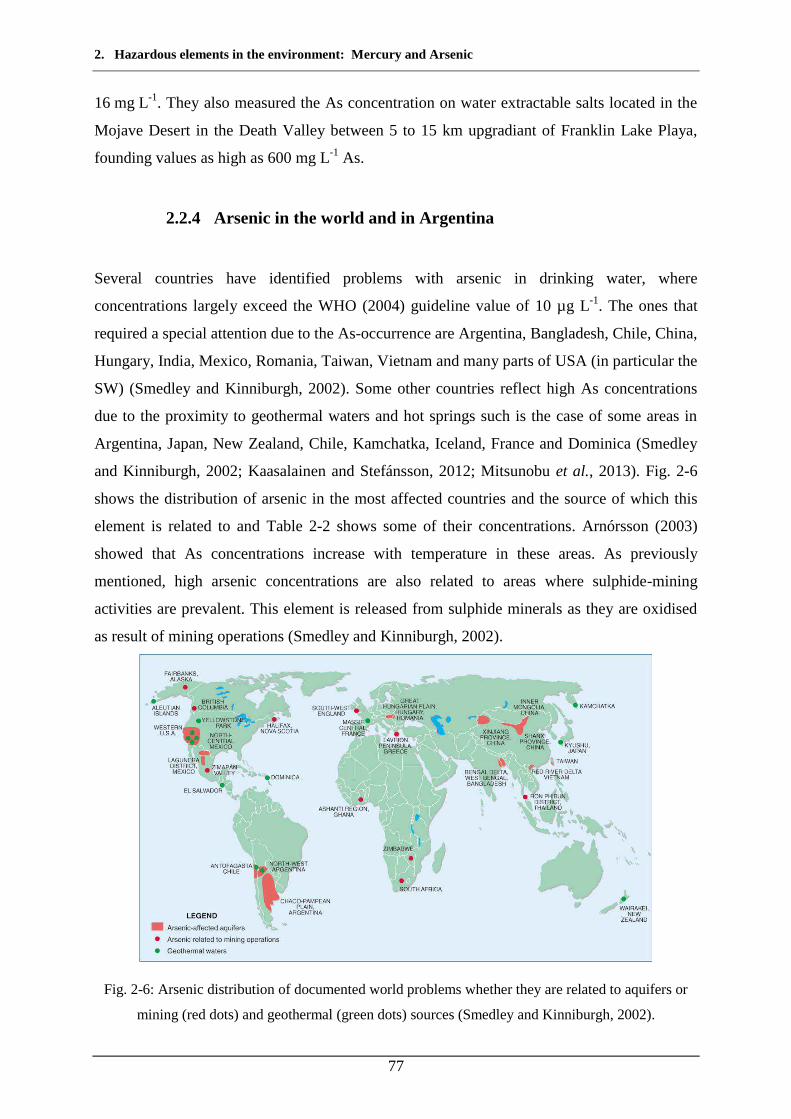
2. Hazardous elements in the environment: Mercury and Arsenic
77
16 mg L-1. They also measured the As concentration on water extractable salts located in the
Mojave Desert in the Death Valley between 5 to 15 km upgradiant of Franklin Lake Playa,
founding values as high as 600 mg L-1 As.
2.2.4 Arsenic in the world and in Argentina
Several countries have identified problems with arsenic in drinking water, where
concentrations largely exceed the WHO (2004) guideline value of 10 µg L-1. The ones that
required a special attention due to the As-occurrence are Argentina, Bangladesh, Chile, China,
Hungary, India, Mexico, Romania, Taiwan, Vietnam and many parts of USA (in particular the
SW) (Smedley and Kinniburgh, 2002). Some other countries reflect high As concentrations
due to the proximity to geothermal waters and hot springs such is the case of some areas in
Argentina, Japan, New Zealand, Chile, Kamchatka, Iceland, France and Dominica (Smedley
and Kinniburgh, 2002; Kaasalainen and Stefánsson, 2012; Mitsunobu et al., 2013). Fig. 2-6
shows the distribution of arsenic in the most affected countries and the source of which this
element is related to and Table 2-2 shows some of their concentrations. Arnórsson (2003)
showed that As concentrations increase with temperature in these areas. As previously
mentioned, high arsenic concentrations are also related to areas where sulphide-mining
activities are prevalent. This element is released from sulphide minerals as they are oxidised
as result of mining operations (Smedley and Kinniburgh, 2002).
Fig. 2-6: Arsenic distribution of documented world problems whether they are related to aquifers or
mining (red dots) and geothermal (green dots) sources (Smedley and Kinniburgh, 2002).
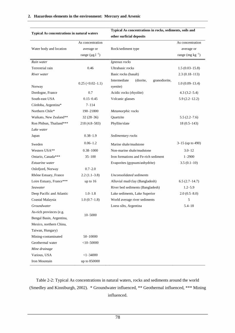
2. Hazardous elements in the environment: Mercury and Arsenic
78
Typical As concentrations in natural waters
Typical As concentrations in rocks, sediments, soils and
other surficial deposits
Water body and location
As concentration
average or
range (µg.l -1)
Rock/sediment type
As concentration
average or
range (mg kg -1)
Rain water
Igneous rocks
Terrestrial rain 0.46
Ultrabasic rocks 1.5 (0.03–15.8)
River water
Basic rocks (basalt) 2.3 (0.18–113)
Norway 0.25 (<0.02–1.1)
Intermediate (diorite, granodiorite,
syenite) 1.0 (0.09–13.4)
Dordogne, France 0.7
Acidic rocks (rhyolite) 4.3 (3.2–5.4)
South-east USA 0.15–0.45
Volcanic glasses 5.9 (2.2–12.2)
Córdoba, Argentina* 7–114
Northern Chile* 190–21800
Metamorphic rocks
Waikato, New Zealand** 32 (28–36)
Quartzite 5.5 (2.2–7.6)
Ron Phibun, Thailand*** 218 (4.8–583)
Phyllite/slate 18 (0.5–143)
Lake water
Japan 0.38–1.9
Sedimentary rocks
Sweden 0.06–1.2
Marine shale/mudstone 3–15 (up to 490)
Western USA** 0.38–1000
Non-marine shale/mudstone 3.0–12
Ontario, Canada*** 35–100
Iron formations and Fe-rich sediment 1–2900
Estuarine water
Evaporites (gypsum/anhydrite) 3.5 (0.1–10)
Oslofjord, Norway 0.7–2.0
Rhône Estuary, France 2.2 (1.1–3.8)
Unconsolidated sediments
Loire Estuary, France*** up to 16
Alluvial mud/clay (Bangladesh) 6.5 (2.7–14.7)
Seawater
River bed sediments (Bangladesh) 1.2–5.9
Deep Pacific and Atlantic 1.0–1.8
Lake sediments, Lake Superior 2.0 (0.5–8.0)
Coastal Malaysia 1.0 (0.7–1.8)
World average river sediments 5
Groundwater
Loess silts, Argentina 5.4–18
As-rich provinces (e.g.
Bengal Basin, Argentina, 10–5000
Mexico, northern China,
Taiwan, Hungary)
Mining-contaminated 50–10000
Geothermal water <10–50000
Mine drainage
Various, USA <1–34000
Iron Mountain up to 850000
Table 2-2: Typical As concentrations in natural waters, rocks and sediments around the world
(Smedley and Kinniburgh, 2002). * Groundwater influenced, ** Geothermal influenced, *** Mining
influenced.
2. Hazardous elements in the environment: Mercury and Arsenic
79
The case in Argentina
In Argentina, numerous studies have been carried out concerning the presence of arsenic in
groundwater and the risk that it could present to human health. The Chaco Pampean Plain that
includes the provinces of Córdoba, La Pampa, Santa Fe, Buenos Aires and Tucumán in
particular, is one of the largest regions in the world (around 1x10⁶ km2) that presents As
issues (Smedley and Kinniburgh, 2002; Nicolli et al., 2012). Such is the case that the
permissible drinking water intake was lowered from 50 to 10 µg L-1 As in 2007 (CAA) to
coincide with that one stipulated by the WHO.
Aquifers in the Chaco Pampean Plain are included in sequences of several hundred meters
composed of clastic sediments that form a system of interconnected multilayer aquifers that
overlie the crystalline basement. Usually this basement presents a faulted system with
ascending and descending blocks of granites, metamorphic rocks and basalts that act as
aquifuge. The hydrogeological system is composed in the base by thick marine pelitic
sediments (green clays from Miocene with very low permeability - aquiclude), hosting very
saline Na-sulfate-chloride type waters. Above this and at a regional scale, lies a very thick
sequence of heterogeneous deposits of aeolian loess and loess-like sediments from the Pampa
Formation (PlioPleistocene) (Nicolli et al., 2012).
During the Pleistocene there was a cold, arid environment that reigned in the Argentina
Cordillera that allowed efficient production of fine silt by periglacial processes (Smedley et
al., 2002). These fine sediments were transported by the dominant winds from the WSW
(Zárate, 2003). Some authors (Raychowdhuy et al., 2013 and references therein) have studied
the composition of the Pampean loess concluding that they present mainly plagioclase and
orthoclase feldspars, volcanic glass shards, quartz, and muscovite and the coarser fraction
contains fragments of metamorphic and acid plutonic rocks mirroring the composition of the
Andean rocks (Gaiero, 2007; Maher et al., 2010). Francisca and Carro Perez (2009) have
shown that especially the sand and silt fractions present a very high content of volcanic glass
(Fig. 2-7). Nevertheless, in the loess of the Chaco-Pampean Plain the silt fraction prevails
over the clay fraction.
In the Holocene the loess deposits have been substantially reworked by aeolian and fluvial
processes. There is also evidence of post-depositional alteration with formation of carbonate
cementation, secondary Mn oxide (as nodules and cement) and soil-forming processes. Thus
evidencing significant climatic variations during the Quaternary in the region (Kröhling and
Iriondo, 1999; Smedley et al., 2002).
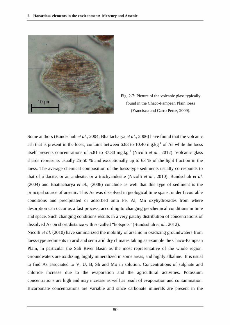
2. Hazardous elements in the environment: Mercury and Arsenic
80
Fig. 2-7: Picture of the volcanic glass typically
found in the Chaco-Pampean Plain loess
(Francisca and Carro Perez, 2009).
Some authors (Bundschuh et al., 2004; Bhattacharya et al., 2006) have found that the volcanic
ash that is present in the loess, contains between 6.83 to 10.40 mg.kg-1 of As while the loess
itself presents concentrations of 5.81 to 37.30 mg.kg-1 (Nicolli et al., 2012). Volcanic glass
shards represents usually 25-50 % and exceptionally up to 63 % of the light fraction in the
loess. The average chemical composition of the loess-type sediments usually corresponds to
that of a dacite, or an andesite, or a trachyandesite (Nicolli et al., 2010). Bundschuh et al.
(2004) and Bhattacharya et al., (2006) conclude as well that this type of sediment is the
principal source of arsenic. This As was dissolved in geological time spans, under favourable
conditions and precipitated or adsorbed onto Fe, Al, Mn oxyhydroxides from where
desorption can occur as a fast process, according to changing geochemical conditions in time
and space. Such changing conditions results in a very patchy distribution of concentrations of
dissolved As on short distance with so called “hotspots” (Bundschuh et al., 2012).
Nicolli et al. (2010) have summarized the mobility of arsenic in oxidizing groundwaters from
loess-type sediments in arid and semi arid dry climates taking as example the Chaco-Pampean
Plain, in particular the Salí River Basin as the most representative of the whole region.
Groundwaters are oxidizing, highly mineralized in some areas, and highly alkaline. It is usual
to find As associated to V, U, B, Sb and Mo in solution. Concentrations of sulphate and
chloride increase due to the evaporation and the agricultural activities. Potassium
concentrations are high and may increase as well as result of evaporation and contamination.
Bicarbonate concentrations are variable and since carbonate minerals are present in the
2. Hazardous elements in the environment: Mercury and Arsenic
81
sediments, carbonate reactions strongly controls the groundwater chemistry. SiO2
concentrations vary in a wide range reflecting the presence of silicate minerals and the highly
soluble amorphous volcanic glass. High pH groundwaters respond to the reaction of silicate
minerals. In the Córdoba area, high grade of special variability in groundwater chemistry and
minor/trace element concentrations over short distances, indicate groundwater flow with poor
mixing (Nicolli et al., 1989). High pH values favour the dissolution of volcanic glass and
leaching of volcanic-origin material in loess-type aquifer sediments. As is likely adsorbed
under circum-neutral pH conditions on Fe/Mn (hydr)oxides, which are hosted as cement or as
coatings on lithic fragments in the loess sediments. Mobilization by desorption is produced
under high pH conditions when As, V, U, F and B anions or oxyanions are released. Those
groundwaters are mostly of the bicarbonate type and their chemical characteristics are highly
controlled by carbonate equilibria
The mineralogical composition of loess is represented by K-mica, clay minerals (kaolinite,
Ca-montmorillonite, illite and chlorite) and frequent Fe- and Al oxides and oxi-hydroxides
(hematite, goethite, Fe(OH)3(a), gibbsite) forming thing coatings over silicate grains.

3. Materials and methods
83
3. Materials and methods

3. Materials and methods
84
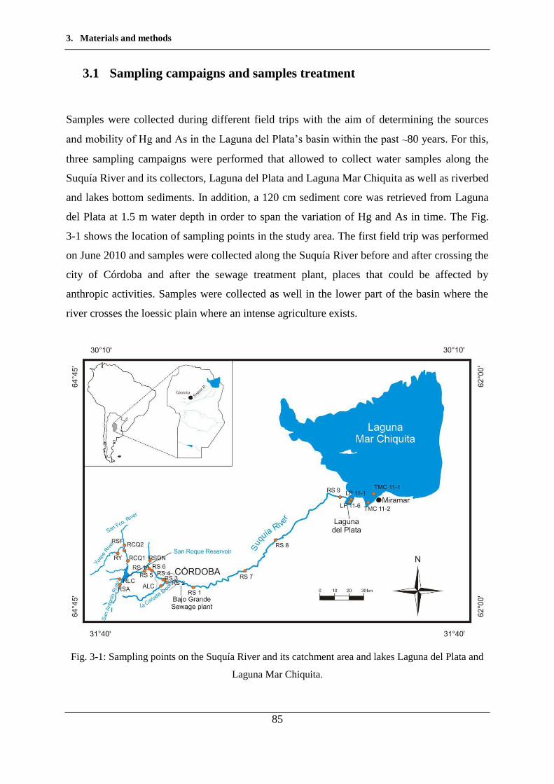
3. Materials and methods
85
3.1 Sampling campaigns and samples treatment
Samples were collected during different field trips with the aim of determining the sources
and mobility of Hg and As in the Laguna del Plata’s basin within the past ~80 years. For this,
three sampling campaigns were performed that allowed to collect water samples along the
Suquía River and its collectors, Laguna del Plata and Laguna Mar Chiquita as well as riverbed
and lakes bottom sediments. In addition, a 120 cm sediment core was retrieved from Laguna
del Plata at 1.5 m water depth in order to span the variation of Hg and As in time. The Fig.
3-1 shows the location of sampling points in the study area. The first field trip was performed
on June 2010 and samples were collected along the Suquía River before and after crossing the
city of Córdoba and after the sewage treatment plant, places that could be affected by
anthropic activities. Samples were collected as well in the lower part of the basin where the
river crosses the loessic plain where an intense agriculture exists.
Fig. 3-1: Sampling points on the Suquía River and its catchment area and lakes Laguna del Plata and
Laguna Mar Chiquita.
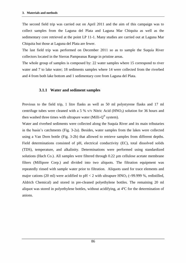
3. Materials and methods
86
The second field trip was carried out on April 2011 and the aim of this campaign was to
collect samples from the Laguna del Plata and Laguna Mar Chiquita as well as the
sedimentary core retrieved at the point LP 11-1. Many studies are carried out at Laguna Mar
Chiquita but those at Laguna del Plata are fewer.
The last field trip was performed on December 2011 so as to sample the Suquía River
collectors located in the Sierras Pampeanas Range in pristine areas.
The whole group of samples is composed by: 22 water samples where 15 correspond to river
water and 7 to lake water; 18 sediments samples where 14 were collected from the riverbed
and 4 from both lake bottom and 1 sedimentary core from Laguna del Plata.
3.1.1 Water and sediment samples
Previous to the field trip, 1 litre flasks as well as 50 ml polystyrene flasks and 17 ml
centrifuge tubes were cleaned with a 5 % v/v Nitric Acid (HNO3) solution for 36 hours and
then washed three times with ultrapure water (Milli-Q® system).
Water and riverbed sediments were collected along the Suquía River and its main tributaries
in the basin’s catchments (Fig. 3-2a). Besides, water samples from the lakes were collected
using a Van Dorn bottle (Fig. 3-2b) that allowed to retrieve samples from different depths.
Field determinations consisted of pH, electrical conductivity (EC), total dissolved solids
(TDS), temperature, and alkalinity. Determinations were performed using standardized
solutions (Hach Co.). All samples were filtered through 0.22 µm cellulose acetate membrane
filters (Millipore Corp.) and divided into two aliquots. The filtration equipment was
repeatedly rinsed with sample water prior to filtration. Aliquots used for trace elements and
major cations (20 ml) were acidified to pH < 2 with ultrapure HNO3 (99.999 %, redistilled,
Aldrich Chemical) and stored in pre-cleaned polyethylene bottles. The remaining 20 ml
aliquot was stored in polyethylene bottles, without acidifying, at 4ºC for the determination of
anions.
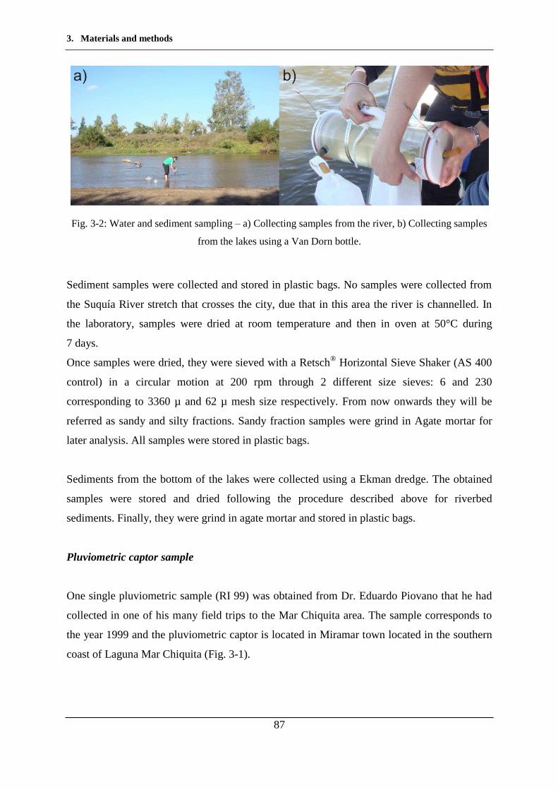
3. Materials and methods
87
Fig. 3-2: Water and sediment sampling – a) Collecting samples from the river, b) Collecting samples
from the lakes using a Van Dorn bottle.
Sediment samples were collected and stored in plastic bags. No samples were collected from
the Suquía River stretch that crosses the city, due that in this area the river is channelled. In
the laboratory, samples were dried at room temperature and then in oven at 50°C during
7 days.
Once samples were dried, they were sieved with a Retsch® Horizontal Sieve Shaker (AS 400
control) in a circular motion at 200 rpm through 2 different size sieves: 6 and 230
corresponding to 3360 µ and 62 µ mesh size respectively. From now onwards they will be
referred as sandy and silty fractions. Sandy fraction samples were grind in Agate mortar for
later analysis. All samples were stored in plastic bags.
Sediments from the bottom of the lakes were collected using a Ekman dredge. The obtained
samples were stored and dried following the procedure described above for riverbed
sediments. Finally, they were grind in agate mortar and stored in plastic bags.
Pluviometric captor sample
One single pluviometric sample (RI 99) was obtained from Dr. Eduardo Piovano that he had
collected in one of his many field trips to the Mar Chiquita area. The sample corresponds to
the year 1999 and the pluviometric captor is located in Miramar town located in the southern
coast of Laguna Mar Chiquita (Fig. 3-1).

3. Materials and methods
88
3.1.2 Sediment core
One sediment core was retrieved from Laguna del Plata (LP 11-1, Lat. 30°54'48.4''S;
Long. 62°51'16.4''W), using a Eijkelkamp core sampler type Beeker (Fig. 3-3a,b) , and a PVC
tube of 65 mm diameter and 120 cm long. After extraction the core was stored at 4°C. Right
after the opening the core was sliced longitudinally in two. One of the parts was photographed
and a high-resolution 256 grey-level image was acquired with the X-ray imaging system
SCOPIX; the other half of the core was sampled every 5 mm (Fig. 3-3c,d).
An average of 7.6 g of sample were placed in previously weighted acrylic boxes (1.8 cm3) and
dried in the oven at 50°C until constant weight was obtained. All samples were grind in agate
mortar and stored in plastic flasks for its later analysis.
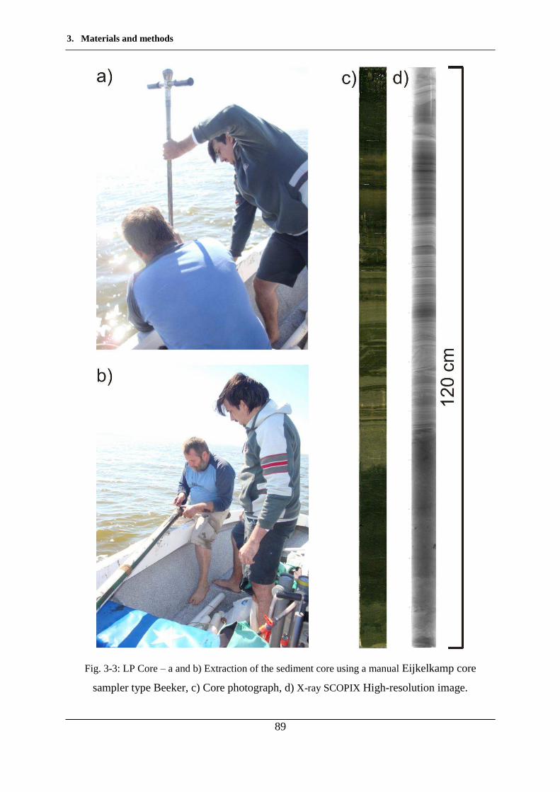
3. Materials and methods
89
Fig. 3-3: LP Core – a and b) Extraction of the sediment core using a manual Eijkelkamp core
sampler type Beeker, c) Core photograph, d) X-ray SCOPIX High-resolution image.
3. Materials and methods
90
3.2 Analytical Methods
3.2.1 Core dating – Radionuclides
Dating technique using 210Pb was first employed in 1973 by Koide et al. (1973) and widely
spread since for marine and lacustrine sediments. The 210Pb (T1/2 = 22.3 years) is a naturally
occurring radionuclide delivered continuously to the landscape by atmospheric fallout (Saari
et al., 2010) and becomes rapidly and strongly bound to particulate matter. This
atmospherically derived 210Pb scavenged by particles, is referred to 210Pb in excess (210Pbxs) of
that supported within particles by the decay of its parent isotope, 226Ra. Another radionuclide,
the 232Th, occurs naturally and usually is associated to the detrital fraction (van der Klooster et
al., 2011), therefore a change in its activity could indicate different lithological sources or
proportions. On the other hand, 137Cs (T1/2 = 30 years) is an artificial radionuclide resulting
from the atmospheric fallout of the nuclear weapon tests during 1953-1963 and the Chernobyl
reactor fire in 1986 (United Nations Scientific Committee on the Effects of Atomic Radiation,
2000; Appleby, 2001). As 210Pb is present in all environments (Ivanovich and Harmon, 1992),
it has been used as an environmental radiotracer of many processes, such as ocean
biogeochemistry, atmospheric deposition and contamination, sedimentary processes and
sediment radiochronology (Sánchez-Cabeza and Ruiz-Fernández, 2012 and references
therein) in recent sediments of a century or so where there is not an equilibrium between 210Pb
and 226Ra (Koide et al., 1973; Sánchez-Cabeza and Ruiz-Fernández, 2012). In systems that
have remained closed for sufficient time ( 150 years), supported 210Pb is in equilibrium with
its parent radionuclide 226Ra (T1/2 = 1600 years) (Sánchez-Cabeza and Ruiz-Fernández, 2012).
As most of the superficial sediment is under mixing due to physical or biological processes,
many authors (Robbins and Edgington, 1975; Carroll et al., 1999; Appleby, 2001; Smith,
2001, Oguri et al., 2012) suggest that it is important to validate 210Pb dates using an
independent time marker as 137Cs that can provide an unambiguous time-stratigraphic
horizon. For this purpose 210Pb, 232Th, 226Ra and 137Cs activities were measured using a low
background, high efficiency, well-shaped detector (CANBERRA) (Schmidt et al, 2009).
The detector was calibrated using certified reference materials (IAEA-RGU-1; IAEA-
RGTh; SOIL-6). Activities were expressed in mBq g-1 and errors are based on 1 SD counting
3. Materials and methods
91
statistics. Excess 210Pb (210Pbxs) was calculated by subtracting the activity supported by its
parent isotope, 226Ra, from the total 210Pb activity in the sediment.
Several models exist in order to obtain an age model, section/layer age as a function of the
depth, accumulation rates or estimate sediment mixing rates. Sánchez-Cabeza and Ruiz-
Fernández (2012) have summarized the existing models in:
Constant Activity model (CA – Former Constant Initial Concentration CIC). The hypothesis is
based that the 210Pbxs concentration when the section i is formed is constant with a value
denoted as C0:
Ci (t = 0) = k ≡ C0 (Eq. 2)
Where k = .
With fi is the main flux to sediment surface;
r is the mass accumulation rate (MAR).
Constant Sedimentation model (CS). It is based on the hypothesis that the mass accumulation
rate r is constant (both for sections and layers). It can be only used if the values of fluxes to
the sediments surface fi are known during a period of about 100 years. With the radioactive
decay and mi as the dry mass of the section, the equation could be written as: (Eq. 3)
Constant Flux model (CF). Widely known as Constant Rate of Supply model (CRS) has its
fundamental hypothesis in that the 210Pbxs flux to the sediment surface is constant (fi = f(i) = k).
Where f(i) is the flux to the sediment surface when layer (i) is formed.
Constant Flux Constant Sedimentation model (CFCS). This model incorporates
simultaneously the CF model hypothesis of constant flux to the sediment surface (fi = f(i) = f)
and the CS model of constant mass accumulation rate (r i = r (i) = r):
(Eq. 4)
3. Materials and methods
92
When the CFCS hypotheses are met, a purely exponential decrease of Ci with the depth
should be observed. Finally, the equation can be solved through a linear regression between
the logarithm of 210Pbxs concentration (ln Ci) and the mass depth mi:
(Eq. 5)
3.2.2 Selective extractions
It is widely known that the toxicity and mobility of pollutants depend strongly on their
specific chemical forms and on their binding states (Gleyzes at al., 2002). Therefore, the
identification of the main binding sites and phase associations of trace elements in soils helps
to understand the geochemical processes in order to evaluate the remobilization potential and
risks induced (Sutherland et al., 2000)
Selective extractions are commonly used in order to determine trace elements distribution in
different solid phases (soils and sediments) based on the rational use of a series of more or
less selective reagents chosen to solubilise successively the different mineralogical fractions
thought to be the responsible for retaining the larger part of the trace metals. The objective is
to simulate various possible natural and anthropogenic modifications of environmental
conditions (Gleyzes et al., 2002 and references therein).
A very well defined protocol was done by Tessier et al. (1979) where the same sample is
treated with the different reagents and the amount of the extracted metal is measured on the
extractant reagent. Another method is the parallel extraction schemes (e.g. Audry et al. 2005)
which is the one applied in this study. It consists of assessing the Hg distribution by 3 parallel
or single chemical extractions, i.e using each reagent on a different sample aliquot (Farrah and
Pickering, 1993; Alborés et al., 2000). Using this second technique, some limitations are
avoided such as (i) metal transfer from one phase to the another (Bemond, 1992), (ii) multiple
risks of sample contamination from successive reagents used (Quevauviller, 1998), (iii)
possible changes in elemental speciation during the successive extraction steps and (iv)
changes or losses of elemental species during the residue washing step (Rosenberg and
Ariese, 2001). Besides, this method shows no risk for sample losses and an error occurred
during one extraction does not compromise the entire schema (Tack et al., 1996).
3. Materials and methods
93
Before the extraction, all solutions were prepared with analytical reagent grade chemicals and
purified water (Milli-Q® system). Labware in contact with the samples was acid clean (soaked
in 10 % HCl during 3 days, rinsed 3 times with Milli-Q® water and dried under a laminar flow
hood). Once that the extraction was done, the solid residue was washed three times with
Milli-Q ® water, tubes were centrifugated for 15 minutes at 3000 rpm to collect the residual
sediment that afterwards they was dried on stove at 50°C, grind in Agate mortar weighted
and analyzed.
3.2.2.1 Ascorbate extraction
This reducing single extraction removes trace elements associated with Mn oxides and the
most reactive Fe oxide fraction (i.e. amorphous oxides; Kostka and Luther III, 1994; Audry et
al., 2006), using a 0.11 M ascorbate reagent (5:5:2 sodium
citrate/sodium-bicarbonate/ascorbic-acid mixture; J.T. Baker, Baker analyzed/J.T. Baker,
Baker analyzed/Acrôs Organics). For this extraction, 12.5 ml of ascorbate solution and 200
mg of dry sediment were added into a 50 ml previously HCl cleaned Teflon® centrifuge tubes
and were placed for 24 h in a rotary shaker at 12 rpm.
3.2.2.2 H2O2 extraction
The oxidizing single extraction using hydrogen peroxide (H2O2) typically attacks organic
matter but sulphides are also partially oxidized during this step (Tessier et al., 1979). This
work utilises a modified Tessier protocol (Ma and Uren, 1995, Audry et al., 2006), previously
applied for Hg solid speciation (Castelle et al. 2007).
For this, 8 ml of 30 % H2O2 (J.T. Baker, Baker analyzed), buffered to pH 5 with NaOH (J.T.
Baker, Baker analyzed), were added to 250 mg of dry sediment in 50 ml Teflon® centrifuge
tubes (Nalgene, Oak-Ridge). The tubes were then placed in an oven at 85°C for 5 h with
manual agitation every 10 min and 3 ml of 30 % H2O2 and 5 ml of 5 M ammonium acetate
(complexing agent, J.T. Baker, Baker analyzed) were added after 3 h. Then, the tubes were
shaken for 30 min (Sahuquillo et al., 2003; Castelle et al. 2007).
3. Materials and methods
94
3.2.2.3 HCl extraction
The so-called reactive (HCl 1N acid-soluble) fraction comprises metals associated with
amorphous and crystalline Mn and Fe oxides, carbonates, hydrous Al silicates (Huerta-Diaz
and Morse 1990, 1992) and acid volatile sulphides (AVS) not including the oxidation
products of Fe monosulphides (goethite and hematite; Raiswell et al., 1994). The acid-soluble
fraction was also empirically designated to extract most of the potentially bioavailable trace
metals (Bryan and Langston, 1992; Langston et al., 1999). For this, 200 mg of dry sediment
and 12.5 ml of HCl 1N were placed in previously HCl cleaned Teflon® centrifuge tubes and
then placed in a rotary shaker for 24 h at 12 rpm (Castelle et al., 2007). Once the extraction
was finished, the pH of the supernatant was measured.
3.2.2.4 Total attack
In this attack, the crystalline matrix of the suspended matter is digested with acid leaving
metals in the solution for analysis. This procedure was carried out in three stages and in this
occasion the material was previously cleaned with HNO3 10 % during three days, washed
three times with Milli-Q water and dried in hood under laminar flux.
Stage 1: Attack
Grounded samples were weighted and 30 mg were placed on attack tubes. To this, 750 µl of
suprapur® HNO3, 1.5 ml of suprapur® HCl and 2.5 ml of suprapur® HF were added. The
tubes were covered with watch glasses and placed in a hot plate at 110°C for 2 h.
Stage 2: Evaporation
After samples cooled, the watch glass was removed and rinsed with Milli-Q water. The tubes
were replaced on the hot plate at 110°C for 6 h to evaporate the water and the acids.
Stage 3: Recovery
In this step, 250 µl of suprapur® HNO3 and 5 ml of Milli-Q water were added to the
evaporation residue. The tubes were closed and replaced on the hot plate at 65°C for 30 mn to
3. Materials and methods
95
accelerate the dissolution. Once the solution cooled, 3.5 ml of supernatant and 6.4 ml of
Milli-Q water were placed on a 10 ml tubes and stored for later analysis.
From these attacks two kind of samples were obtained: the solid residue (reducible fraction -
Hgasc, oxidisable fraction - and acid-soluble/reactive fraction - HgHCl) and the
supernatants fractions (ascorbate, HCl and total). All of them were stored and kept for further
analyses.
3.2.3 Mineral characterization
3.2.3.1 Granulometry
Sample sizes determinations were performed with a laser granulometer Malvern Mastersizer S
(Fig. 3-4) in the EPOC laboratory (Université de Bordeaux 1).
The particles to be measured were diluted in a beaker of 0.6 to 1 litre and then put into
circulation in traversed cell crossed by parallel laser beam. Particles illuminated by the laser
deviate the light from its main axis. The amount of deflected light and the extent of the
deflection of the angle allow to measure the particle size. Thus, larger particles sizes deviate
significant amounts of light on low angles while small particles deviate tiny amounts of light
but on wider angles. Intensities received at different angles by the detector are digitized and
analyzed by calculation using the Mie theory (Mie, 1908). This mathematical theory,
interpreting the light scattered by a particle, is modelled for solid spheres. That is to say that
the particles are treated as equivalent spheres. The calculation result is shown as a distribution
curve of particles (http://lecob.obs-banyuls.fr). Laser micro-granulometry gives a distribution
of particle volume. The analytical range varies approximately between 0.05µm - 900µm.
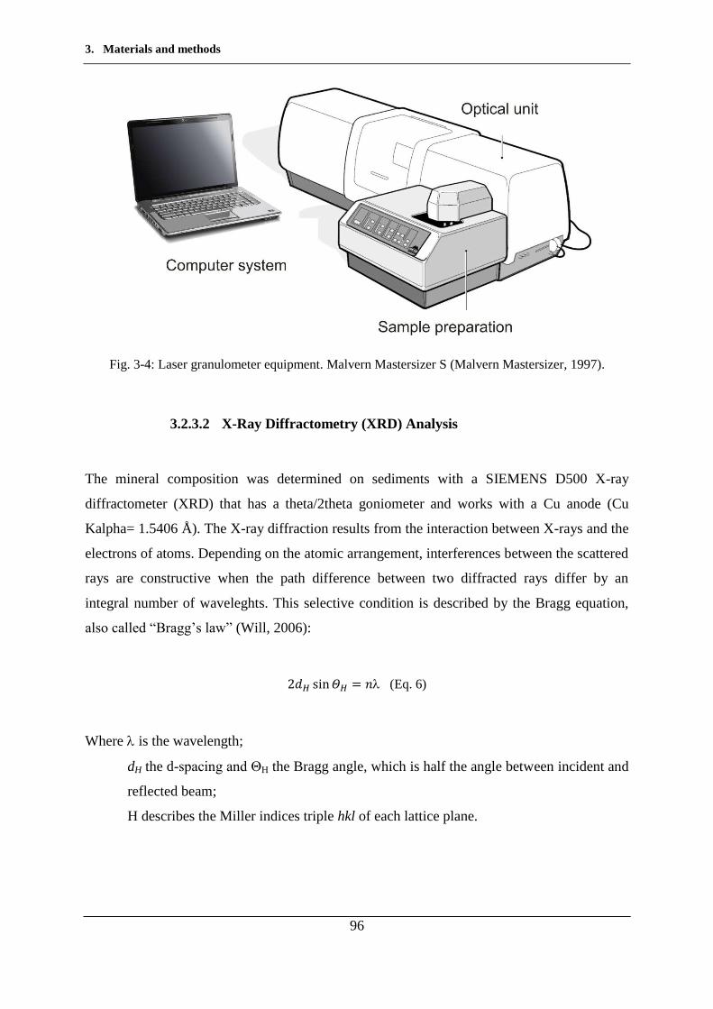
3. Materials and methods
96
Fig. 3-4: Laser granulometer equipment. Malvern Mastersizer S (Malvern Mastersizer, 1997).
3.2.3.2 X-Ray Diffractometry (XRD) Analysis
The mineral composition was determined on sediments with a SIEMENS D500 X-ray
diffractometer (XRD) that has a theta/2theta goniometer and works with a Cu anode (Cu
Kalpha= 1.5406 Å). The X-ray diffraction results from the interaction between X-rays and the
electrons of atoms. Depending on the atomic arrangement, interferences between the scattered
rays are constructive when the path difference between two diffracted rays differ by an
integral number of waveleghts. This selective condition is described by the Bragg equation,
also called “Bragg’s law” (Will, 2006):
(Eq. 6)
Where is the wavelength;
dH the d-spacing and ΘH the Bragg angle, which is half the angle between incident and
reflected beam;
H describes the Miller indices triple hkl of each lattice plane.
3. Materials and methods
97
This method provides information such as types and nature of crystalline phases present or
structural make-up of phases. It consists in irradiating a material with a parallel beam of
monochromatic X-rays. The atomic lattice of the sample acts as a three dimensional
diffraction grating causing the X-ray beam to be diffracted to specific angles. The diffraction
pattern, that includes position (angles) and intensities of the diffracted beam, provides
information about the sample. In case of pure phase, the diffractogram obtained is always the
same and can be described by Miller indices (Warren, 1969; Klug and Alexander, 1974). The
diffraction spectrum consists of a plot that reflects intensities in the y axis and the 2Θ detector
angle in the x axis.
Samples were previously dried and were not orientated. The analysis was performed between
4 and 90° of 2Θ with a scan step of 0.02° and a step duration of 2 seconds.
3.2.3.3 X-Ray Fluorescence (XRF) analysis
Some major and minor elements (Al, Si, K, Ti, Fe, Zr, Mn, Sr, S, Cl and Ca) were measured
on one of the halves of the core through X-ray fluorescence (XRF) with an Avaatech XRF
Core – Scanner with a 1mm resolution. The equipment uses a 58 kV X-ray voltage and an
X-ray current of 10 mA. This is a well-established analytical technique for estimating the
composition of rocks and sediments (Ramsey et al., 1995; Jenkins, 1999; De Vries and
Vrebos, 2002).
The principle of XRF analysis is based on excitation of electrons by incident X-radiation.
Ejection of electrons from inner atomic shells creates vacancies which are filled by electrons
falling back from the outer shells, whereby surplus energy is emitted as a pulse of secondary
X-radiation. Emitted fluorescence energy and wavelength spectra are characteristic for atoms
of specific elements, which permit estimation of their relative abundances (Jansen et al.,
1998; Wien et al., 2005; Ge et al., 2005; Weltje and Tjallingii, 2008). This is an increasingly
accepted method as an effective way of obtaining high-resolution elemental records because
of its non-destructive and nearly continuous measurements (Croudace et al., 2006; Jansen et
al., 1998; Rothwell and Rack, 2006; Thomson et al., 2006). Environmental changes,
diagenetic processes and pollutant inputs can be deduced by elemental variations determined
by XRF core scanning, as well as it can assist in sediment correlation and process studies
(Rothwell and Rack, 2006). The measurements obtained by XRF reflect the composition of a
3. Materials and methods
98
thin (sub-mm) layer on top of the sediment surface where the intensities of the different
elements are expressed as counts per second (cps). The counts should be proportional to the
concentration of the element in the sediment but the signal might be attenuated or enhanced
by the presence and concentrations of other elements (Löwemark et al., 2011; Liang et al.,
2012). Fluctuations along the core do not necessarily mean that there has been an increase or
decrease in the flux of a certain element. Usually these variations are given by the deposition
rate of the diluting agent, which in lakes it is often the organic matter. This effect is handled
by using a conservative element for normalizing. The use of Al for this purpose allows to
address the relative variations in the lithogenic component of the sediment (Löwemark et al.,
2011). Water content, surface roughness and grain size variations are other sedimentary
factors that have an influence over XRF measurements (Böning et al., 2007, Tjallingii et al,
2007; Weltje and Tjallingi, 2008).
3.2.4 Chemical characterization
3.2.4.1 Measurements of pH
The pH values were measured in 1:10 suspensions prepared with samples collected every 5
mm along the LP core using a multi-parameter analyzer (pH meter Consort C561, previously
calibrated).
3.2.4.2 Total and Organic Carbon and sulphur
Total and Organic Carbon (Corg) and sulphur were determined on sediments of the LP core
using a carbon/sulphur LECO CS 125 analyzer (Fig. 3-5a). For the Corg analysis, samples
were previously acidified in crucibles (Fig. 3-5b) with 2N HCl to destroy carbonates, and then
dried at 60°C for 24 hours to remove inorganic C and most of the remaining acid and water
(Etcheber et al., 1999).
During measurement, an almost complete oxidation of compounds occurs by combustion at
850°C in an induction furnace under an oxygen flow. The oxygen stream carries the oxidized
compounds (SO2 and CO) into a first infrared cell where SO2 is detected. The SO2 and CO
compounds are oxidized again through a catalyst (Cu/Pt). The SO3 formed from SO2 is
captured by a cellulose trap while the CO2 formed from CO is carried to a second infrared
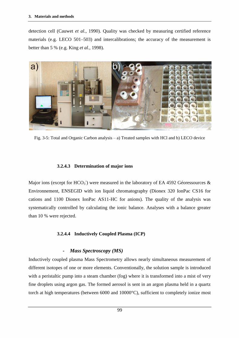
3. Materials and methods
99
detection cell (Cauwet et al., 1990). Quality was checked by measuring certified reference
materials (e.g. LECO 501–503) and intercalibrations; the accuracy of the measurement is
better than 5 % (e.g. King et al., 1998).
Fig. 3-5: Total and Organic Carbon analysis – a) Treated samples with HCl and b) LECO device
3.2.4.3 Determination of major ions
Major ions (except for HCO3-) were measured in the laboratory of EA 4592 Géoressources &
Environnement, ENSEGID with ion liquid chromatography (Dionex 320 IonPac CS16 for
cations and 1100 Dionex IonPac AS11-HC for anions). The quality of the analysis was
systematically controlled by calculating the ionic balance. Analyses with a balance greater
than 10 % were rejected.
3.2.4.4 Inductively Coupled Plasma (ICP)
- Mass Spectroscopy (MS)
Inductively coupled plasma Mass Spectrometry allows nearly simultaneous measurement of
different isotopes of one or more elements. Conventionally, the solution sample is introduced
with a peristaltic pump into a steam chamber (fog) where it is transformed into a mist of very
fine droplets using argon gas. The formed aerosol is sent in an argon plasma held in a quartz
torch at high temperatures (between 6000 and 10000°C), sufficient to completely ionize most
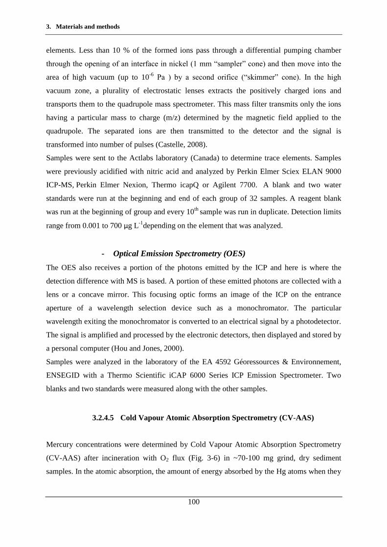
3. Materials and methods
100
elements. Less than 10 % of the formed ions pass through a differential pumping chamber
through the opening of an interface in nickel (1 mm “sampler” cone) and then move into the
area of high vacuum (up to 10-6 Pa ) by a second orifice (“skimmer” cone). In the high
vacuum zone, a plurality of electrostatic lenses extracts the positively charged ions and
transports them to the quadrupole mass spectrometer. This mass filter transmits only the ions
having a particular mass to charge (m/z) determined by the magnetic field applied to the
quadrupole. The separated ions are then transmitted to the detector and the signal is
transformed into number of pulses (Castelle, 2008).
Samples were sent to the Actlabs laboratory (Canada) to determine trace elements. Samples
were previously acidified with nitric acid and analyzed by Perkin Elmer Sciex ELAN 9000
ICP-MS, Perkin Elmer Nexion, Thermo icapQ or Agilent 7700. A blank and two water
standards were run at the beginning and end of each group of 32 samples. A reagent blank
was run at the beginning of group and every 10th sample was run in duplicate. Detection limits
range from 0.001 to 700 µg L-1depending on the element that was analyzed.
- Optical Emission Spectrometry (OES)
The OES also receives a portion of the photons emitted by the ICP and here is where the
detection difference with MS is based. A portion of these emitted photons are collected with a
lens or a concave mirror. This focusing optic forms an image of the ICP on the entrance
aperture of a wavelength selection device such as a monochromator. The particular
wavelength exiting the monochromator is converted to an electrical signal by a photodetector.
The signal is amplified and processed by the electronic detectors, then displayed and stored by
a personal computer (Hou and Jones, 2000).
Samples were analyzed in the laboratory of the EA 4592 Géoressources & Environnement,
ENSEGID with a Thermo Scientific iCAP 6000 Series ICP Emission Spectrometer. Two
blanks and two standards were measured along with the other samples.
3.2.4.5 Cold Vapour Atomic Absorption Spectrometry (CV-AAS)
Mercury concentrations were determined by Cold Vapour Atomic Absorption Spectrometry
(CV-AAS) after incineration with O2 flux (Fig. 3-6) in ~70-100 mg grind, dry sediment
samples. In the atomic absorption, the amount of energy absorbed by the Hg atoms when they
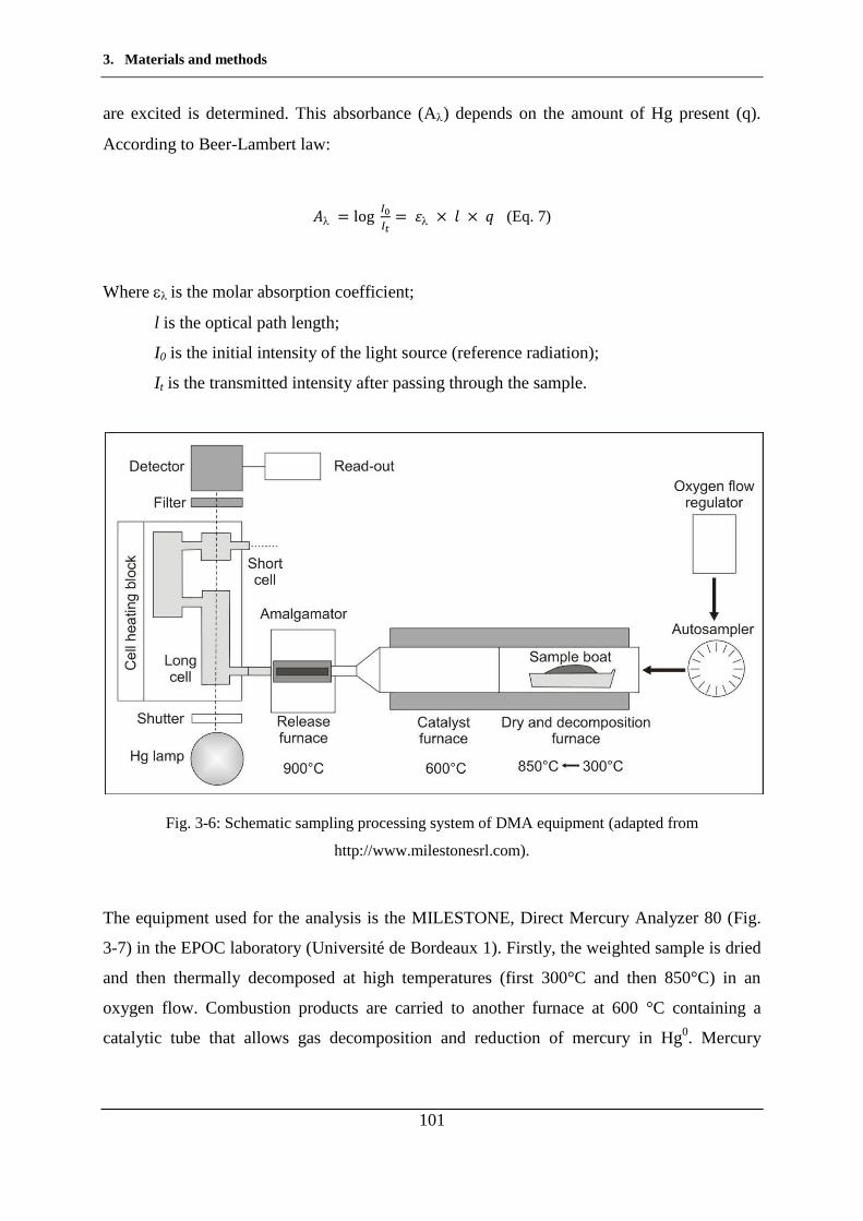
3. Materials and methods
101
are excited is determined. This absorbance (A ) depends on the amount of Hg present (q).
According to Beer-Lambert law:
(Eq. 7)
Where is the molar absorption coefficient;
l is the optical path length;
I0 is the initial intensity of the light source (reference radiation);
It is the transmitted intensity after passing through the sample.
Fig. 3-6: Schematic sampling processing system of DMA equipment (adapted from
http://www.milestonesrl.com).
The equipment used for the analysis is the MILESTONE, Direct Mercury Analyzer 80 (Fig.
3-7) in the EPOC laboratory (Université de Bordeaux 1). Firstly, the weighted sample is dried
and then thermally decomposed at high temperatures (first 300°C and then 850°C) in an
oxygen flow. Combustion products are carried to another furnace at 600 °C containing a
catalytic tube that allows gas decomposition and reduction of mercury in Hg0. Mercury
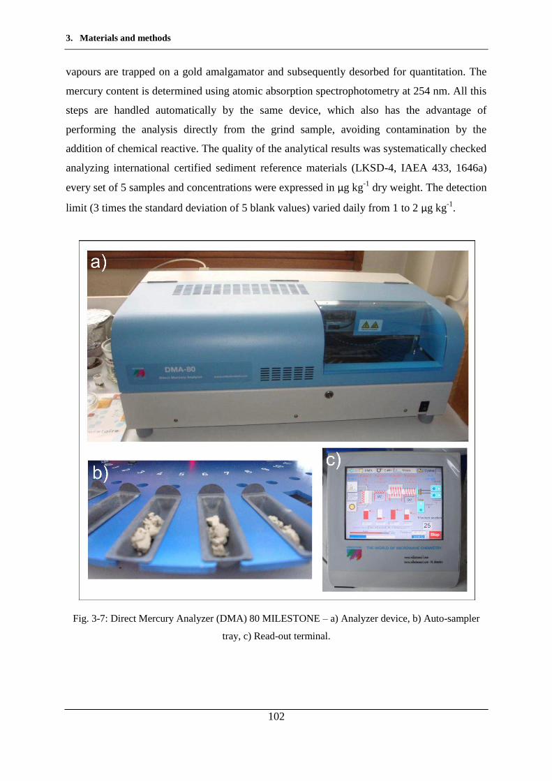
3. Materials and methods
102
vapours are trapped on a gold amalgamator and subsequently desorbed for quantitation. The
mercury content is determined using atomic absorption spectrophotometry at 254 nm. All this
steps are handled automatically by the same device, which also has the advantage of
performing the analysis directly from the grind sample, avoiding contamination by the
addition of chemical reactive. The quality of the analytical results was systematically checked
analyzing international certified sediment reference materials (LKSD-4, IAEA 433, 1646a)
every set of 5 samples and concentrations were expressed in µg kg-1 dry weight. The detection
limit (3 times the standard deviation of 5 blank values) varied daily from 1 to 2 µg kg-1.
Fig. 3-7: Direct Mercury Analyzer (DMA) 80 MILESTONE – a) Analyzer device, b) Auto-sampler
tray, c) Read-out terminal.
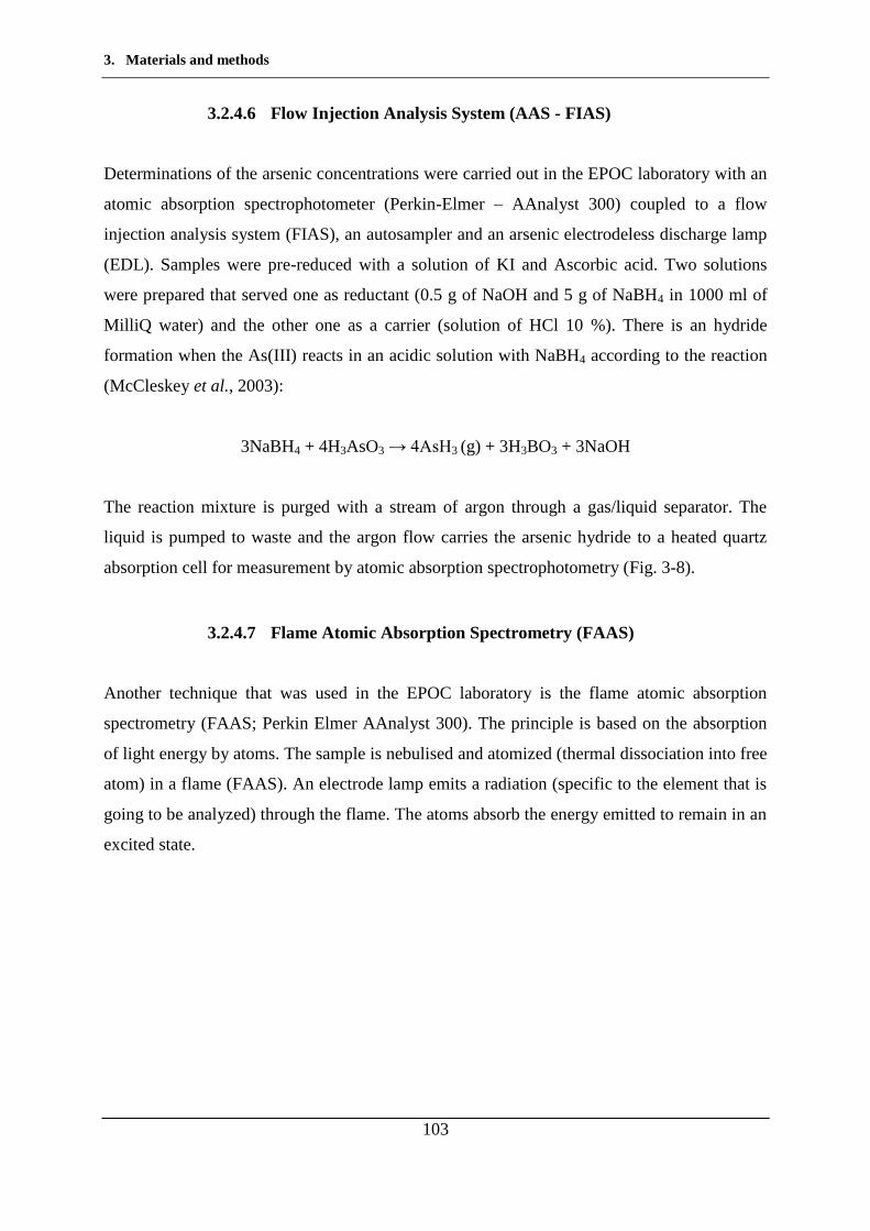
3. Materials and methods
103
3.2.4.6 Flow Injection Analysis System (AAS - FIAS)
Determinations of the arsenic concentrations were carried out in the EPOC laboratory with an
atomic absorption spectrophotometer (Perkin-Elmer – AAnalyst 300) coupled to a flow
injection analysis system (FIAS), an autosampler and an arsenic electrodeless discharge lamp
(EDL). Samples were pre-reduced with a solution of KI and Ascorbic acid. Two solutions
were prepared that served one as reductant (0.5 g of NaOH and 5 g of NaBH4 in 1000 ml of
MilliQ water) and the other one as a carrier (solution of HCl 10 %). There is an hydride
formation when the As(III) reacts in an acidic solution with NaBH4 according to the reaction
(McCleskey et al., 2003):
3NaBH4 + 4H3AsO3 → 4AsH3 (g) + 3H3BO3 + 3NaOH
The reaction mixture is purged with a stream of argon through a gas/liquid separator. The
liquid is pumped to waste and the argon flow carries the arsenic hydride to a heated quartz
absorption cell for measurement by atomic absorption spectrophotometry (Fig. 3-8).
3.2.4.7 Flame Atomic Absorption Spectrometry (FAAS)
Another technique that was used in the EPOC laboratory is the flame atomic absorption
spectrometry (FAAS; Perkin Elmer AAnalyst 300). The principle is based on the absorption
of light energy by atoms. The sample is nebulised and atomized (thermal dissociation into free
atom) in a flame (FAAS). An electrode lamp emits a radiation (specific to the element that is
going to be analyzed) through the flame. The atoms absorb the energy emitted to remain in an
excited state.
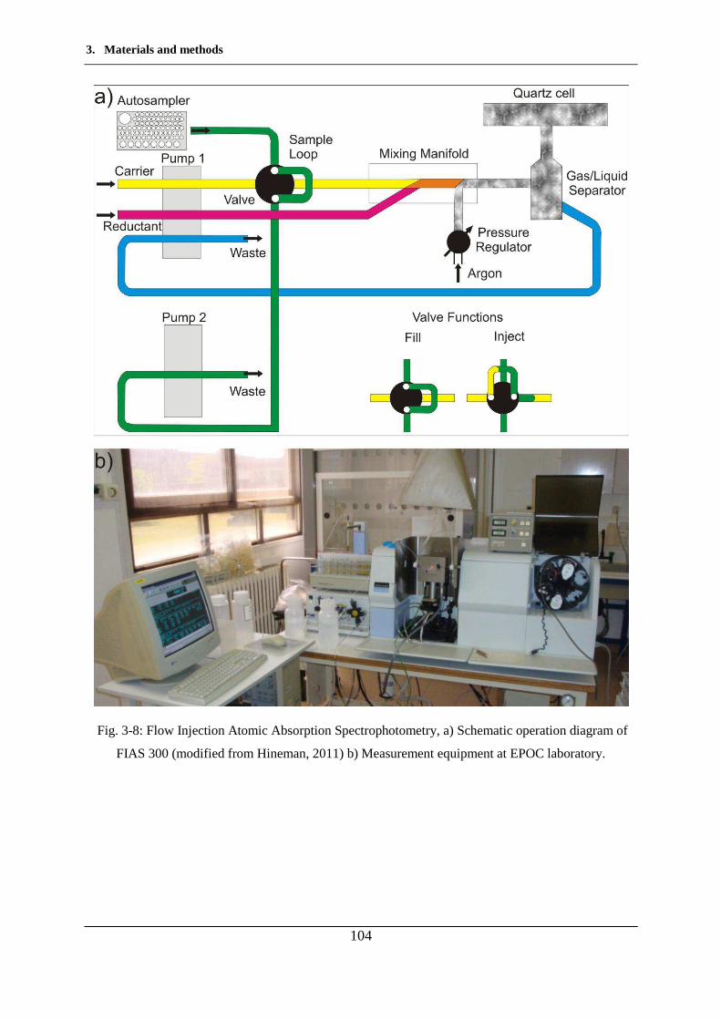
3. Materials and methods
104
Fig. 3-8: Flow Injection Atomic Absorption Spectrophotometry, a) Schematic operation diagram of
FIAS 300 (modified from Hineman, 2011) b) Measurement equipment at EPOC laboratory.
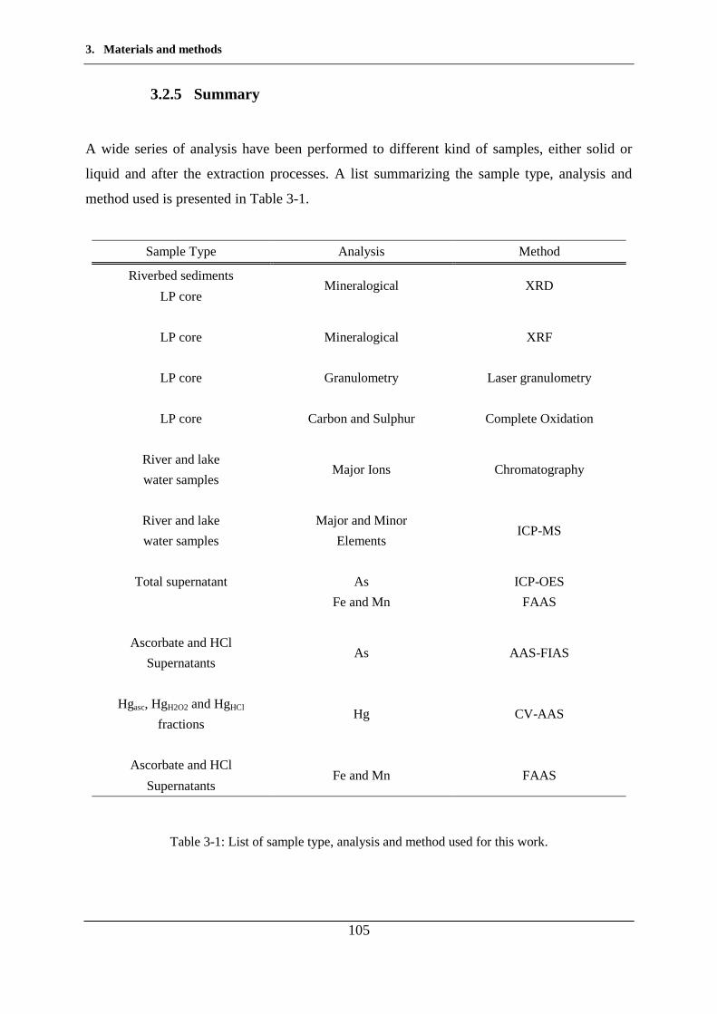
3. Materials and methods
105
3.2.5 Summary
A wide series of analysis have been performed to different kind of samples, either solid or
liquid and after the extraction processes. A list summarizing the sample type, analysis and
method used is presented in Table 3-1.
Sample Type Analysis Method
Riverbed sediments Mineralogical XRD
LP core
LP core Mineralogical XRF
LP core Granulometry Laser granulometry
LP core Carbon and Sulphur Complete Oxidation
River and lake
Major Ions Chromatography water samples
River and lake Major and Minor
ICP-MS water samples Elements
Total supernatant As ICP-OES
Fe and Mn FAAS
Ascorbate and HCl
As AAS-FIAS Supernatants
Hgasc, HgH2O2 and HgHCl
Hg CV-AAS fractions
Ascorbate and HCl
Fe and Mn FAAS Supernatants
Table 3-1: List of sample type, analysis and method used for this work.

3. Materials and methods
106
3.3 Satellite Image treatment
3.3.1 Contributions of satellite images
It is well known that the entire Mar Chiquita system suffers changes in its size due to the
climate changes that originates in South America, as Piovano et al. (2002, 2004a) described
this area as a “sensitive climate indicator”. Beyond that, records that quantify the surface
occupation of this system are scarce. In order to study this change in size satellite images from
Landsat 5 TM (Thematic Mapper), Landsat 7 ETM+ (Enhanced Thematic Mapper Plus) and
the recently launched Landsat 8 LDCM (Landsat Data Continuity Mission - February 11,
2013) images were analyzed with the software ArcGIS version 10.1 (©ESRI 1999-2013).
ArcGIS is a comprehensive system that allows people to collect, organize, manage, analyze,
communicate, and distribute geographic information (http://resources.arcgis.com).
Remote sensing uses the properties of emission and/or reflexion of radiation. These rays are
electromagnetic waves, carrying energy, which propagate without attenuation in the void but
are more or less absorbed in different environments. Solar radiation is the external energy
input to the Earth. A body whose temperature is greater than 0K emits electromagnetic
radiation. It plays the role of source transforming part of the thermal energy into radiant
energy. The fraction of absorbed radiation serves for changing the internal energy of the body
which will result in an emission in another wavelength. There are several Remote Sensing
Systems that register these emissions depending on the wavelength (Fig. 3-9), Girard and
Girard (2010).
The Landsat Program is a serie of Earth-observing satellite missions jointly managed by
NASA and the U.S. Geological Survey (http://landsat.gsfc.nasa.gov/) that started in 1972.
Landsat 5 images are taken with a Thematic Mapper (TM) sensor. These images have data
files that consist of seven spectral bands with a resolution of 30 meters. The Landsat 7 images
were acquired with an Enhanced Thematic Mapper Plus (ETM+) sensor. These images
consist of eight spectral bands with a spatial resolution of 30 meters for bands 1 to 7. The
panchromatic band 8 has a resolution of 15 meters. Landsat 8 is the latest satellite sent and the
one that covers wider spectra. Table 3-2 shows the characteristics for each band and for the
three satellites (5, 7 and 8). All satellites have a 16-day repeat cycle, the approximate scene
3. Materials and methods
107
size is 170 km north-south by 183 km east-west. The map projection is given in the geodetic
system WGS 84 and UTM (Universal Transverse Mercator) projection.
Landsat uses as well the Worldwide Reference System (WRS) where each scene is designated
by a path and a row. Sequential path numbers are from east to west to 233 nominal satellite
orbital tracks, starting with number 001 for the first track which crosses the equator at
64.60 degrees west longitude. Row refers to the latitudinal centre line of a frame of imagery.
As the satellite moves along its path, the observatory instruments are continuously scanning
the terrain below with a 5 per cent overlapping. The combination of a Path number and a Row
number uniquely identifies a nominal scene centre. The study area is covered by the Path 228
and 229 and the Row 081. Images corresponding to the Path 229 that include the westernmost
part of Laguna Mar Chiquita have line gaps hence only images on the path 228 were
analyzed. Images were downloaded with free access from http://landsatlook.usgs.gov/,
spanning a period from 1986 to 2013. Previous satellite images are not available in free
access. Among all the satellite images available, only those who were georeferenced and had
a maximum of cloud cover of 20 % were chosen, making a total of 14 satellite images to
analyze.
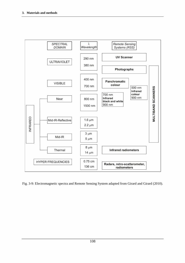
3. Materials and methods
108
Fig. 3-9: Electromagnetic spectra and Remote Sensing System adapted from Girard and Girard (2010).
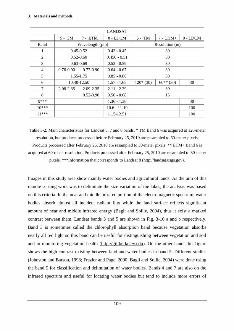
3. Materials and methods
109
LANDSAT
5 - TM 7 - ETM+ 8 - LDCM 5 - TM 7 - ETM+ 8 - LDCM Band Wavelength (µm) Resolution (m)
1 0.45-0.52 0.43 - 0.45 30 2 0.52-0.60 0.450 - 0.51 30 3 0.63-0.69 0.53 - 0.59 30 4 0.76-0.90 0.77-0.90 0.64 - 0.67 30 5 1.55-1.75 0.85 - 0.88 30 6 10.40-12.50 1.57 - 1.65 120* (30) 60** (30) 30 7 2.08-2.35 2.09-2.35 2.11 - 2.29 30 8
0.52-0.90 0.50 - 0.68 15
9***
1.36 - 1.38
30 10***
10.6 - 11.19
100
11***
11.5-12.51
100
Table 3-2: Main characteristics for Landsat 5, 7 and 8 bands. * TM Band 6 was acquired at 120-meter
resolution, but products processed before February 25, 2010 are resampled to 60-meter pixels.
Products processed after February 25, 2010 are resampled to 30-meter pixels. ** ETM+ Band 6 is
acquired at 60-meter resolution. Products processed after February 25, 2010 are resampled to 30-meter
pixels. ***Information that corresponds to Landsat 8 (http://landsat.usgs.gov).
Images in this study area show mainly water bodies and agricultural lands. As the aim of this
remote sensing work was to delimitate the size variation of the lakes, the analysis was based
on this criteria. In the near and middle infrared portion of the electromagnetic spectrum, water
bodies absorb almost all incident radiant flux while the land surface reflects significant
amount of near and middle infrared energy (Bagli and Soille, 2004), thus it exist a marked
contrast between them. Landsat bands 3 and 5 are shown in Fig. 3-10 a and b respectively.
Band 3 is sometimes called the chlorophyll absorption band because vegetation absorbs
nearly all red light so this band can be useful for distinguishing between vegetation and soil
and in monitoring vegetation health (http://gif.berkeley.edu). On the other hand, this figure
shows the high contrast existing between land and water bodies in band 5. Different studies
(Johnston and Barson, 1993; Frazier and Page, 2000; Bagli and Soille, 2004) were done using
the band 5 for classification and delimitation of water bodies. Bands 4 and 7 are also on the
infrared spectrum and useful for locating water bodies but tend to include more errors of
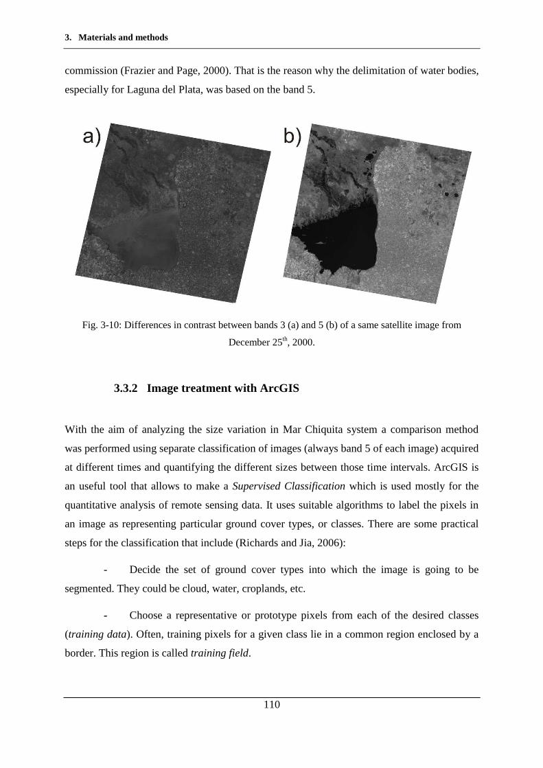
3. Materials and methods
110
commission (Frazier and Page, 2000). That is the reason why the delimitation of water bodies,
especially for Laguna del Plata, was based on the band 5.
Fig. 3-10: Differences in contrast between bands 3 (a) and 5 (b) of a same satellite image from
December 25th, 2000.
3.3.2 Image treatment with ArcGIS
With the aim of analyzing the size variation in Mar Chiquita system a comparison method
was performed using separate classification of images (always band 5 of each image) acquired
at different times and quantifying the different sizes between those time intervals. ArcGIS is
an useful tool that allows to make a Supervised Classification which is used mostly for the
quantitative analysis of remote sensing data. It uses suitable algorithms to label the pixels in
an image as representing particular ground cover types, or classes. There are some practical
steps for the classification that include (Richards and Jia, 2006):
- Decide the set of ground cover types into which the image is going to be
segmented. They could be cloud, water, croplands, etc.
- Choose a representative or prototype pixels from each of the desired classes
(training data). Often, training pixels for a given class lie in a common region enclosed by a
border. This region is called training field.
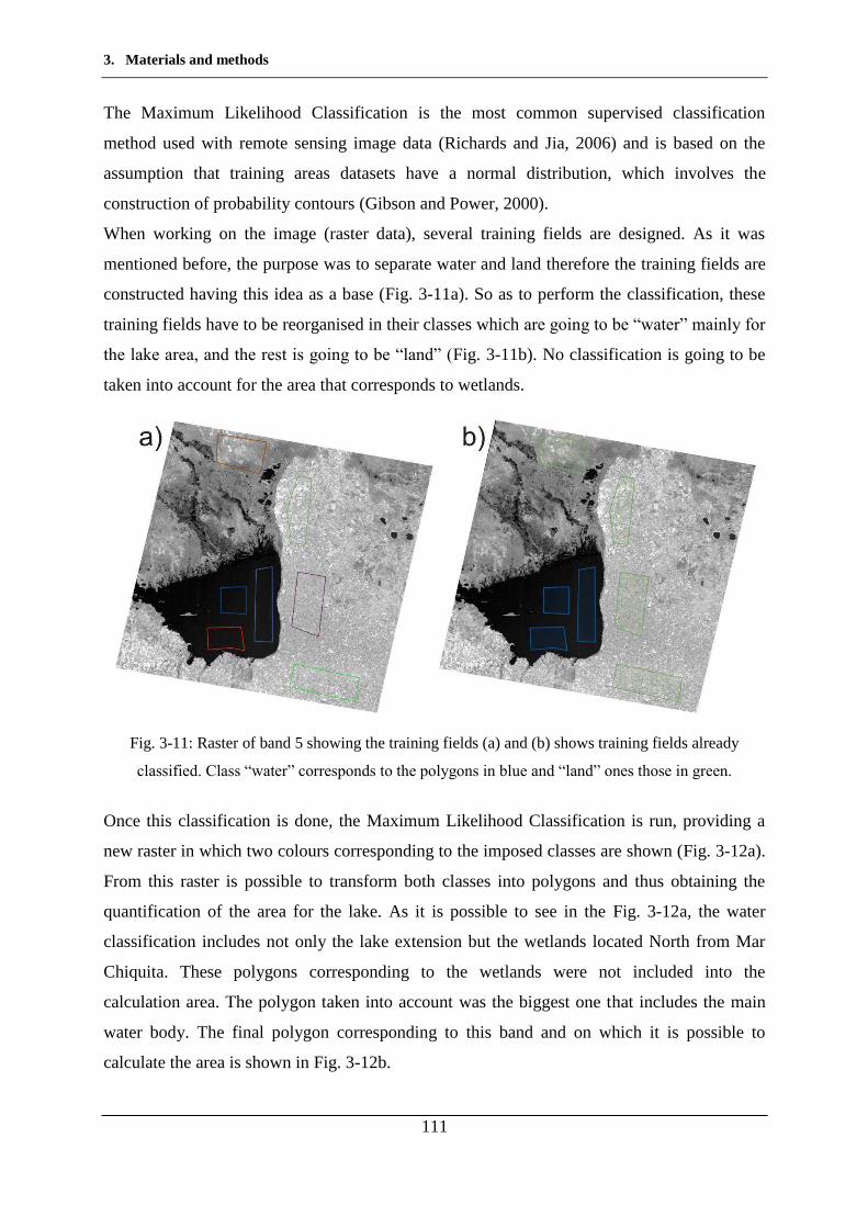
3. Materials and methods
111
The Maximum Likelihood Classification is the most common supervised classification
method used with remote sensing image data (Richards and Jia, 2006) and is based on the
assumption that training areas datasets have a normal distribution, which involves the
construction of probability contours (Gibson and Power, 2000).
When working on the image (raster data), several training fields are designed. As it was
mentioned before, the purpose was to separate water and land therefore the training fields are
constructed having this idea as a base (Fig. 3-11a). So as to perform the classification, these
training fields have to be reorganised in their classes which are going to be “water” mainly for
the lake area, and the rest is going to be “land” (Fig. 3-11b). No classification is going to be
taken into account for the area that corresponds to wetlands.
Fig. 3-11: Raster of band 5 showing the training fields (a) and (b) shows training fields already
classified. Class “water” corresponds to the polygons in blue and “land” ones those in green.
Once this classification is done, the Maximum Likelihood Classification is run, providing a
new raster in which two colours corresponding to the imposed classes are shown (Fig. 3-12a).
From this raster is possible to transform both classes into polygons and thus obtaining the
quantification of the area for the lake. As it is possible to see in the Fig. 3-12a, the water
classification includes not only the lake extension but the wetlands located North from Mar
Chiquita. These polygons corresponding to the wetlands were not included into the
calculation area. The polygon taken into account was the biggest one that includes the main
water body. The final polygon corresponding to this band and on which it is possible to
calculate the area is shown in Fig. 3-12b.
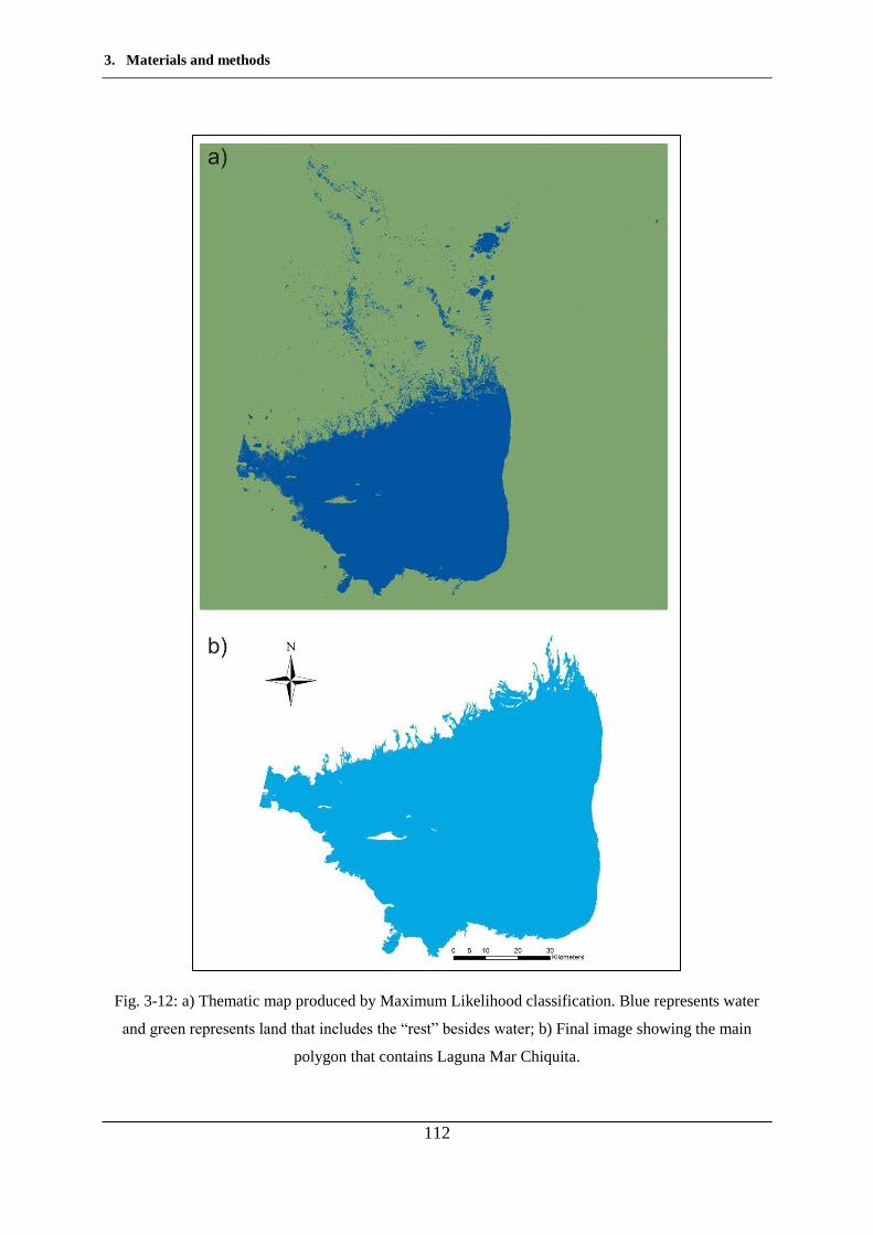
3. Materials and methods
112
Fig. 3-12: a) Thematic map produced by Maximum Likelihood classification. Blue represents water
and green represents land that includes the “rest” besides water; b) Final image showing the main
polygon that contains Laguna Mar Chiquita.
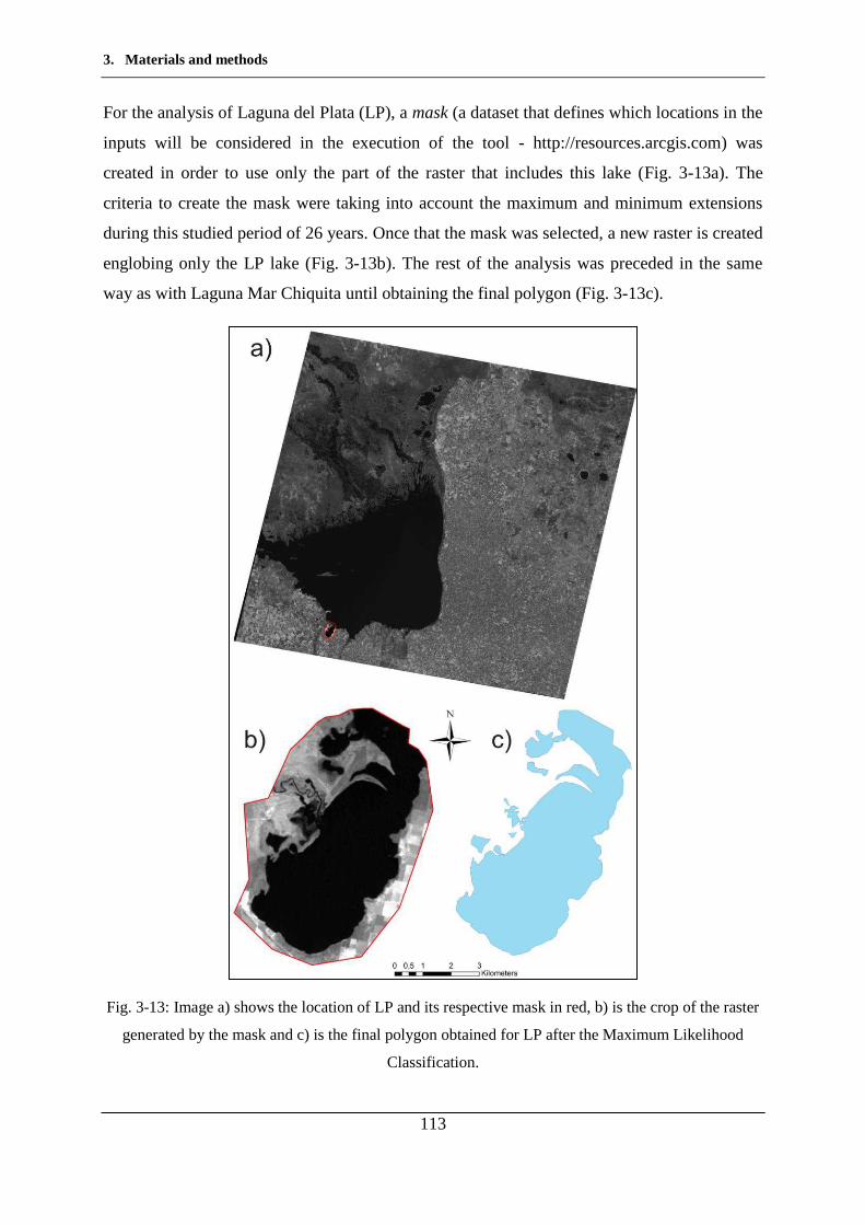
3. Materials and methods
113
For the analysis of Laguna del Plata (LP), a mask (a dataset that defines which locations in the
inputs will be considered in the execution of the tool - http://resources.arcgis.com) was
created in order to use only the part of the raster that includes this lake (Fig. 3-13a). The
criteria to create the mask were taking into account the maximum and minimum extensions
during this studied period of 26 years. Once that the mask was selected, a new raster is created
englobing only the LP lake (Fig. 3-13b). The rest of the analysis was preceded in the same
way as with Laguna Mar Chiquita until obtaining the final polygon (Fig. 3-13c).
Fig. 3-13: Image a) shows the location of LP and its respective mask in red, b) is the crop of the raster
generated by the mask and c) is the final polygon obtained for LP after the Maximum Likelihood
Classification.

4. Results
115
4. Results

4. Results
116
4. Results
117
4.1 Geochemical characterization of the basin
The sources of major dissolved ions (Ca2+, Mg2+, Na+, K+, Cl-, SO42-; HCO3
-) are multiple
such as rainfall inputs, weathering, dissolution of evaporitic minerals or leached during
rainstorms (Garrels and Mackenzie, 1971; Drever, 1988; Stallard, 1995a,b). The deposition
places or sinks are also multiple like lakes or river beds during their drying stage (Gibbs,
1970; Meybeck, 2003) and there is a growing evidence of active recycling of most of major
elements which suggests that each element may have manifold natural sources and sinks
(Likens et al., 1977; Meybeck, 2003). Among the factors that control major ions are climate,
water runoff (that increases weathering), higher lake residence times, tectonic (especially in
recent mountain ranges, rift and/or volcanic regions) (Meybeck, 2003) and lithology, being
this one an essential factor in determining river chemistry (Garrels and Mackenzie, 1971;
Drever, 1988). Human activities in particular mining, chemical industries, urbanization and
agriculture (through the use of fertilizers) have also altered the river chemistry (Meybeck et
al., 1989; Flintrop et al., 1996). Comparisons of regular surveys done from the 1960s with
those of hundred years ago reveal a worldwide increase in Na+, Cl- and SO42- concentrations
due to the anthropogenic impact, whereas Ca2+, Mg2+ and HCO3- concentrations are more
stable (Meybeck et al., 1989; Kimstach et al., 1998). It is widely known that SO42- is a
parameter highly sensitive to anthropic influence.
4.1.1 Aquatic geochemistry
With the aim to evaluate if physicochemical changes occur in the Suquía River basin and the
lakes major ions as well as conductivity, total dissolved solids (TDS), temperature, pH and
dissolved oxygen (DO) were measured. These parameters for the river and lake water samples
are presented in
Table 4-1. A clear geochemical gradient is observed from the catchments to the mouth of the
river. River waters at the basin catchments are diluted and slightly saline near the river mouth
(43 to 1340 µS cm-1). In the lake, waters are highly saline, showing conductivity values that
range from 78100 to 126300 µS cm-1. This trend is also noticeably for the pH values: neutral
pH values predominate in the catchments and they become increasing alkaline downflow,

4. Results
118
ranging from 7.20 to 8.47. Lake waters are markedly alkaline, with pH values ranging from
8.27 to 9.25 (
Table 4-1and Fig. 3-1).
A chemical gradient was also observed in lake water samples for those located near the
surface and in depth. Surface samples were collected at ~20 cm from the surface and those in
depth were collected at ~4 m for samples corresponding to Laguna Mar Chiquita and at
~1.4 m for samples gathered in Laguna del Plata (they are marked with S or D after the
sample name –
Table 4-1). Deeper waters present higher values in conductivity and Total Dissolved Solids
(TDS) for both lakes. In LP, deeper waters present lower pH values and cooler temperatures
that in surface. Dissolved Oxygen also shows lower concentrations in deeper waters near to
the bottom of the lake. Furthermore, major ions present higher concentrations in depth than in
surface except for NH4+.
Following the Piper classification (Fig. 4-1), waters in the basin’s catchments are of the
Ca2+-HCO3- type and they evolve downflow to Na+-Cl--SO4
2- type. Major ion compositions
for 14 samples were also represented on Stiff diagrams (Fig. 4-2) in order to depict the
geographical distribution of these different water types. Before entering to the city of
Córdoba, river waters are of the calcium-bicarbonate-type (RS5 and RS6). Once in the urban
area they change their composition from calcium-sulphate into sodium-sulphate type (RS4,
ALC, RS3, RS2 and RS1) and in the lower part of the basin, waters are clearly of the sodium-
sulphate type with an increment of Na+ and Cl– in samples RS7 and RS8. Concerning lake
waters they are saline to brine waters of a clearly marked sodium-chlorided type.
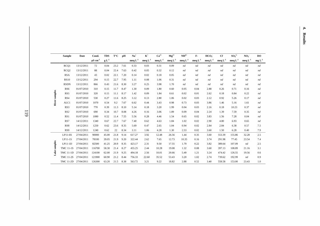
4. Results
119
Sample Date Cond. TDS T°C pH Na+ K + Ca2+ Mg2+ NH4+ F- HCO3- Cl- SO4
2- NO3- DO
µS cm-1 g L-1 meq L-1 meq L-1 meq L-1 meq L-1 meq L-1 meq L-1 meq L-1 meq L-1 meq L-1 meq L-1 mg L-1
Riv
er s
ampl
es
RCQ1 13/12/2011 72 0.04 23.2 7.61 0.33 0.03 0.31 0.09 nd nd nd nd nd nd nd
RCQ2 13/12/2011 88 0.04 22.4 7.63 0.42 0.05 0.32 0.12 nd nd nd nd nd nd nd
RSA 13/12/2011 43 0.02 22.1 7.20 0.14 0.02 0.18 0.05 nd nd nd nd nd nd nd
RS10 13/12/2011 294 0.15 22.7 7.95 1.11 0.08 1.06 0.31 nd nd nd nd nd nd nd
RSDN 13/12/2011 866 0.43 21.6 8.30 3.27 0.25 3.98 1.70 nd nd nd nd nd nd nd
RS6 01/07/2010 310 0.15 11.7 8.47 1.30 0.09 1.80 0.60 0.05 0.04 2.88 0.26 0.71 0.16 nd
RS5 01/07/2010 320 0.15 11.1 8.17 1.42 0.09 1.84 0.61 0.02 0.01 2.62 0.18 0.84 0.22 nd
RS4 01/07/2010 530 0.27 11.6 8.25 3.12 0.13 2.80 1.06 0.02 0.03 2.12 0.92 5.26 0.17 nd
ALC1 01/07/2010 1070 0.54 9.2 7.67 6.62 0.44 3.43 0.98 0.73 0.03 3.86 1.46 5.16 1.61 nd
RS3 01/07/2010 770 0.39 11.3 8.10 5.14 0.18 3.20 1.99 0.04 0.03 2.16 0.18 10.23 0.37 nd
RS2 01/07/2010 690 0.34 10.7 8.08 4.26 0.16 3.06 1.89 0.09 0.04 2.24 1.39 7.59 0.35 nd
RS1 01/07/2010 1080 0.52 11.4 7.55 5.56 0.28 4.46 1.54 0.65 0.02 3.83 1.56 7.28 0.04 nd
RS7 14/12/2011 1340 0.67 22.7 7.67 7.40 0.62 4.63 1.84 1.02 0.02 2.90 4.80 6.93 0.65 nd
RS8 14/12/2011 1250 0.62 23.6 8.35 5.69 0.47 2.65 1.04 0.94 0.02 2.84 2.84 6.38 0.57 7.5
RS9 14/12/2011 1240 0.62 22 8.34 3.11 1.06 4.28 1.30 2.53 0.02 3.60 1.50 6.28 0.40 7.9
Lake
sam
ples
LP11-6S 27/04/2011 90000 45.00 21.8 9.14 617.27 3.92 12.48 26.56 1.44 0.35 3.60 553.39 155.86 32.28 2.5
LP11-1S 27/04/2011 78100 39.05 21.9 9.20 322.44 2.62 7.65 12.73 10.35 0.16 3.74 291.98 77.45 23.54 7.4
LP11-1D 27/04/2011 82500 41.25 20.9 8.35 423.17 2.31 9.50 17.55 1.79 0.22 3.82 389.64 107.09 nd 2.5
TMC 11-1S 27/04/2011 116700 58.30 21.4 8.27 455.25 2.44 10.28 19.08 1.32 0.08 3.60 397.13 108.89 21.16 3.1
TMC 11-1D 27/04/2011 124100 62.00 21.9 9.25 494.18 2.56 10.01 20.66 5.49 1.21 3.24 474.42 126.55 19.56 0.6
TMC 11-2S 27/04/2011 121900 60.90 21.2 8.44 756.33 22.60 35.52 53.43 3.20 1.02 2.74 739.62 192.99 nd 0.9
TMC 11-2D 27/04/2011 126300 63.20 21.5 8.38 563.72 3.21 9.22 18.82 2.88 0.52 3.40 558.58 153.00 23.43 1.0
4. Results
120
Table 4-1: Physicochemical parameters of river and lake water samples. Cond. –
Conductivity, TDS – Total Dissolved Solids. Concentrations of major ions are expressed in
meq L-1. IB: Ionic Balance, DO: dissolved Oxigen nd: not determined.
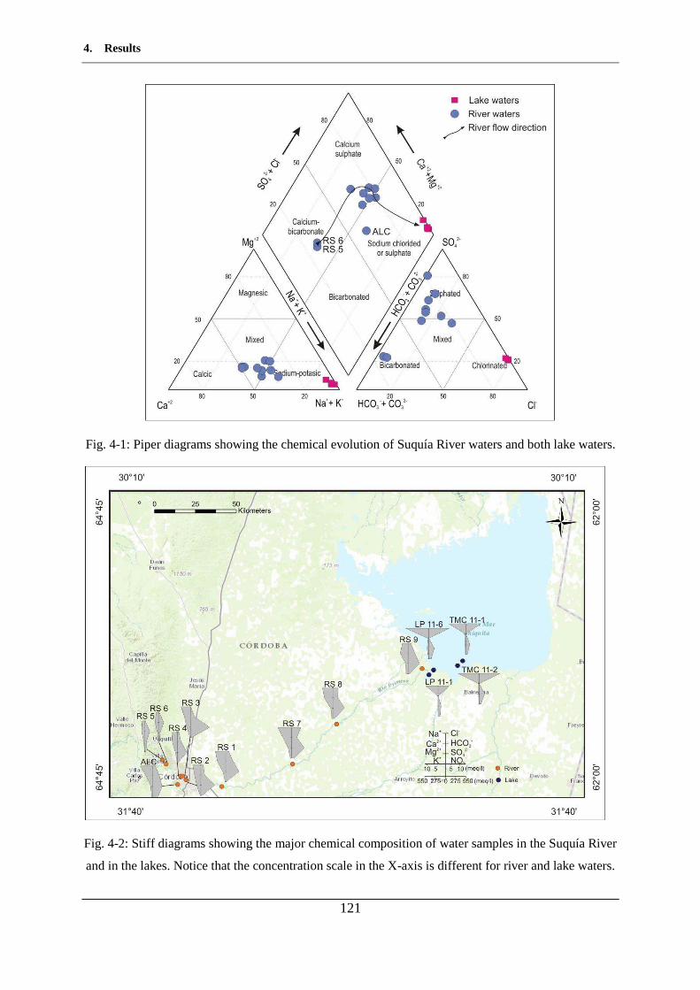
4. Results
121
Fig. 4-1: Piper diagrams showing the chemical evolution of Suquía River waters and both lake waters.
Fig. 4-2: Stiff diagrams showing the major chemical composition of water samples in the Suquía River
and in the lakes. Notice that the concentration scale in the X-axis is different for river and lake waters.

4. Results
122
Saturation indexes were calculated to state the saturation of water samples with respect to
minerals using the geochemical software PHREEQC (Parkhurst and Appelo, 1999) the
following the equation (Eq. 8): (Eq. 8)
Where: SI is the saturation index;
IAP is the Ion Activity Product;
K is the solubility product.
When SI = 0, there is equilibrium between the mineral and the solution, SI 0 reflects
subsaturation and SI 0 supersaturation (Appelo and Postma, 2005). The values obtained for
the Suquía River, Laguna Mar Chiquita and Laguna del Plata (Table 4-2) show that halite and
anhydrite are always subsaturated. Gypsum and fluorite with values clearly 0 are always
subsaturated in river waters but lake waters present mild supersaturation with respect to
gypsum and a stronger supersaturation with respect to fluorite. Dolomite and aragonite are
almost always supersaturated with the exception, in both cases, in samples ALC and RS1. On
the other hand, calcite with values 0 is supersaturated in all samples. The general tendency
shows that the SI values become increasingly positive from the upper part of the basin to the
lake area.
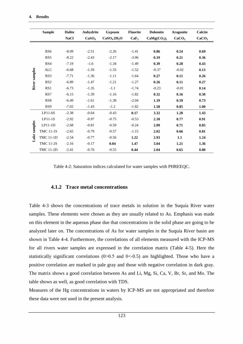
4. Results
123
Sample Halite Anhydrite Gypsum Fluorite Dolomite Aragonite Calcite
NaCl CaSO4 CaSO4˙2H2O CaF2 CaMg(CO3)2 CaCO3 CaCO3
Riv
er s
ampl
es
RS6 -8.09 -2.51 -2.26 -1.41 0.86 0.54 0.69
RS5 -8.22 -2.43 -2.17 -3.06 0.19 0.21 0.36
RS4 -7.19 -1.6 -1.34 -1.49 0.39 0.28 0.43
ALC -6.68 -1.59 -1.33 -1.52 -0.37 -0.02 0.13
RS3 -7.71 -1.36 -1.11 -1.64 0.27 0.11 0.26
RS2 -6.89 -1.47 -1.21 -1.27 0.26 0.11 0.27
RS1 -6.73 -1.35 -1.1 -1.74 -0.23 -0.01 0.14
RS7 -6.15 -1.39 -1.16 -1.82 0.32 0.16 0.30
RS8 -6.49 -1.61 -1.38 -2.04 1.19 0.59 0.73
RS9 -7.02 -1.43 -1.2 -1.82 1.58 0.85 1.00
Lake
sam
ples
LP11-6S -2.38 -0.64 -0.43 0.17 3.32 1.28 1.43
LP11-1S -2.92 -0.97 -0.75 -0.53 2.18 0.77 0.91
LP11-1D -2.68 -0.81 -0.59 -0.24 2.09 0.71 0.85
TMC 11-1S -2.65 -0.79 -0.57 -1.15 2.02 0.66 0.81
TMC 11-1D -2.54 -0.77 -0.56 1.22 2.93 1.1 1.24
TMC 11-2S -2.16 -0.17 0.04 1.47 3.04 1.21 1.36
TMC 11-2D -2.41 -0.76 -0.55 0.44 2.04 0.65 0.80
Table 4-2: Saturation indices calculated for water samples with PHREEQC.
4.1.2 Trace metal concentrations
Table 4-3 shows the concentrations of trace metals in solution in the Suquía River water
samples. These elements were chosen as they are usually related to As. Emphasis was made
on this element in the aqueous phase due that concentrations in the solid phase are going to be
analyzed later on. The concentrations of As for water samples in the Suquía River basin are
shown in Table 4-4. Furthermore, the correlations of all elements measured with the ICP-MS
for all rivers water samples are expressed in the correlation matrix (Table 4-5). Here the
statistically significant correlations (0 0.5 and 0<-0.5) are highlighted. Those who have a
positive correlation are marked in pale gray and those with negative correlation in dark gray.
The matrix shows a good correlation between As and Li , Mg, Si, Ca, V, Br, Sr, and Mo. The
table shows as well, as good correlation with TDS.
Measures of the Hg concentrations in waters by ICP-MS are not appropriated and therefore
these data were not used in the present analysis.
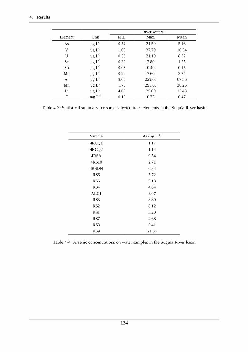
4. Results
124
River waters Element Unit Min. Max. Mean
As µg L-1 0.54 21.50 5.16
V µg L-1 1.00 37.70 10.54
U µg L-1 0.53 21.10 8.02
Se µg L-1 0.30 2.80 1.25
Sb µg L-1 0.03 0.49 0.15
Mo µg L-1 0.20 7.60 2.74
Al µg L-1 8.00 229.00 67.56
Mn µg L-1 1.70 295.00 38.26
Li µg L-1 4.00 25.00 13.48
F mg L-1 0.10 0.75 0.47
Table 4-3: Statistical summary for some selected trace elements in the Suquía River basin
Sample As (µg L-1)
4RCQ1 1.17
4RCQ2 1.14
4RSA 0.54
4RS10 2.71
4RSDN 6.34
RS6 5.72
RS5 3.13
RS4 4.84
ALC1 9.07
RS3 8.80
RS2 8.12
RS1 3.20
RS7 4.68
RS8 6.41
RS9 21.50
Table 4-4: Arsenic concentrations on water samples in the Suquía River basin
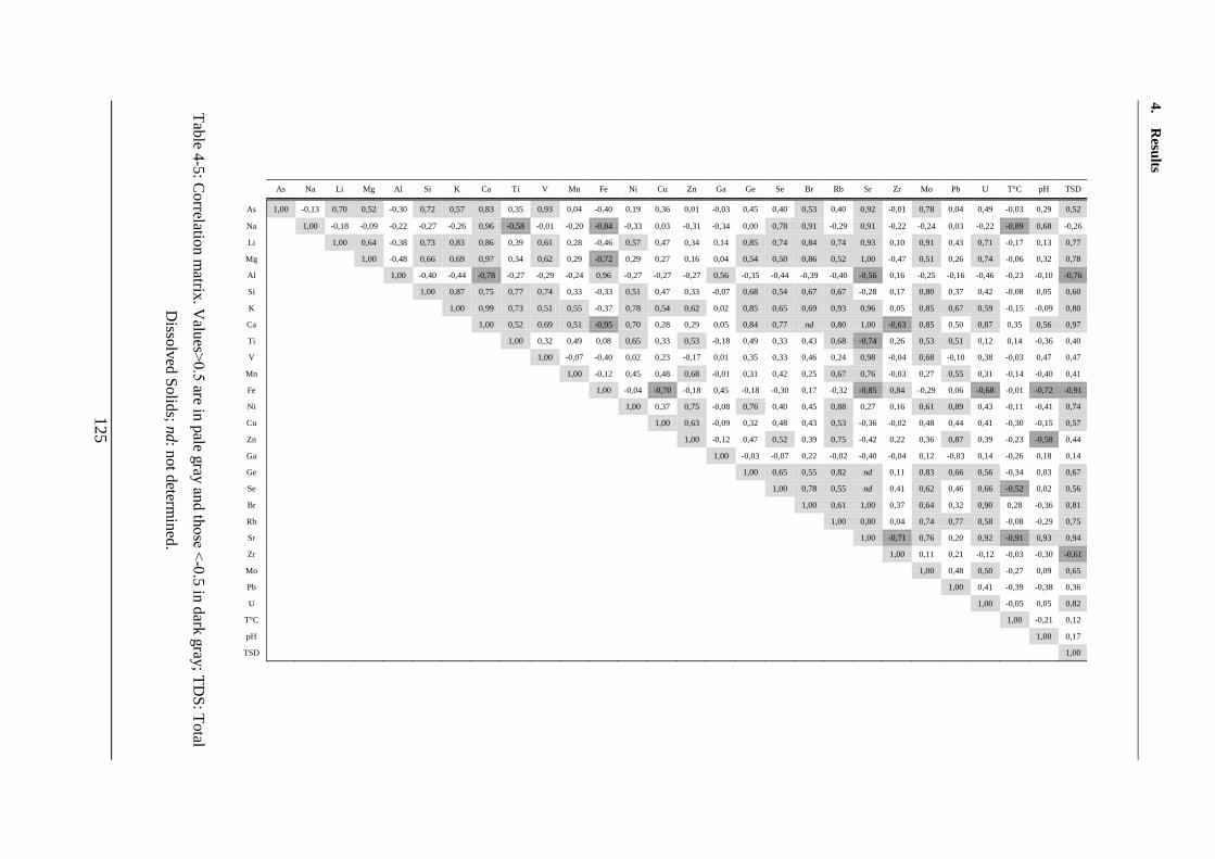
4. Results
125
Table 4-5: C
orrelation matrix. V
alues0.5 are in pale gray and those -0.5 in dark gray; T
DS
: Total
Dissolved S
olids; nd: not determined
.
As Na Li Mg Al Si K Ca Ti V Mn Fe Ni Cu Zn Ga Ge Se Br Rb Sr Zr Mo Pb U T°C pH TSD
As 1,00 -0,13 0,70 0,52 -0,30 0,72 0,57 0,83 0,35 0,93 0,04 -0,40 0,19 0,36 0,01 -0,03 0,45 0,40 0,53 0,40 0,92 -0,01 0,78 0,04 0,49 -0,03 0,29 0,52
Na
1,00 -0,18 -0,09 -0,22 -0,27 -0,26 0,96 -0,58 -0,01 -0,20 -0,84 -0,33 0,03 -0,31 -0,34 0,00 0,78 0,91 -0,29 0,91 -0,22 -0,24 0,03 -0,22 -0,89 0,68 -0,26
Li
1,00 0,64 -0,38 0,73 0,83 0,86 0,39 0,61 0,28 -0,46 0,57 0,47 0,34 0,14 0,85 0,74 0,84 0,74 0,93 0,10 0,91 0,43 0,71 -0,17 0,13 0,77
Mg
1,00 -0,48 0,66 0,69 0,97 0,34 0,62 0,29 -0,72 0,29 0,27 0,16 0,04 0,54 0,50 0,86 0,52 1,00 -0,47 0,51 0,26 0,74 -0,06 0,32 0,78
Al
1,00 -0,40 -0,44 -0,78 -0,27 -0,29 -0,24 0,96 -0,27 -0,27 -0,27 0,56 -0,35 -0,44 -0,39 -0,40 -0,56 0,16 -0,25 -0,16 -0,46 -0,23 -0,10 -0,76
Si
1,00 0,87 0,75 0,77 0,74 0,33 -0,33 0,51 0,47 0,33 -0,07 0,68 0,54 0,67 0,67 -0,28 0,17 0,80 0,37 0,42 -0,08 0,05 0,60
K
1,00 0,99 0,73 0,51 0,55 -0,37 0,78 0,54 0,62 0,02 0,85 0,65 0,69 0,93 0,96 0,05 0,85 0,67 0,59 -0,15 -0,09 0,80
Ca
1,00 0,52 0,69 0,51 -0,95 0,70 0,28 0,29 0,05 0,84 0,77 nd 0,80 1,00 -0,63 0,85 0,50 0,87 0,35 0,56 0,97
Ti
1,00 0,32 0,49 0,08 0,65 0,33 0,53 -0,18 0,49 0,33 0,43 0,68 -0,74 0,26 0,53 0,51 0,12 0,14 -0,36 0,40
V
1,00 -0,07 -0,40 0,02 0,23 -0,17 0,01 0,35 0,33 0,46 0,24 0,98 -0,04 0,68 -0,10 0,38 -0,03 0,47 0,47
Mn
1,00 -0,12 0,45 0,48 0,68 -0,01 0,31 0,42 0,25 0,67 0,76 -0,03 0,27 0,55 0,31 -0,14 -0,40 0,41
Fe
1,00 -0,04 -0,70 -0,18 0,45 -0,18 -0,30 0,17 -0,32 -0,85 0,84 -0,29 0,06 -0,68 -0,01 -0,72 -0,91
Ni
1,00 0,37 0,75 -0,08 0,76 0,40 0,45 0,88 0,27 0,16 0,61 0,89 0,43 -0,11 -0,41 0,74
Cu
1,00 0,63 -0,09 0,32 0,48 0,43 0,53 -0,36 -0,02 0,48 0,44 0,41 -0,30 -0,15 0,57
Zn
1,00 -0,12 0,47 0,52 0,39 0,75 -0,42 0,22 0,36 0,87 0,39 -0,23 -0,58 0,44
Ga
1,00 -0,03 -0,07 0,22 -0,02 -0,40 -0,04 0,12 -0,03 0,14 -0,26 0,18 0,14
Ge
1,00 0,65 0,55 0,82 nd 0,11 0,83 0,66 0,56 -0,34 0,03 0,67
Se
1,00 0,78 0,55 nd 0,41 0,62 0,46 0,66 -0,52 0,02 0,56
Br
1,00 0,61 1,00 0,37 0,64 0,32 0,90 0,28 -0,36 0,81
Rb
1,00 0,80 0,04 0,74 0,77 0,58 -0,08 -0,29 0,75
Sr
1,00 -0,71 0,76 0,20 0,92 -0,91 0,93 0,94
Zr
1,00 0,11 0,21 -0,12 -0,03 -0,30 -0,61
Mo
1,00 0,48 0,50 -0,27 0,09 0,65
Pb
1,00 0,41 -0,39 -0,38 0,36
U
1,00 -0,05 0,05 0,82
T°C
1,00 -0,21 0,12
pH
1,00 0,17
TSD 1,00
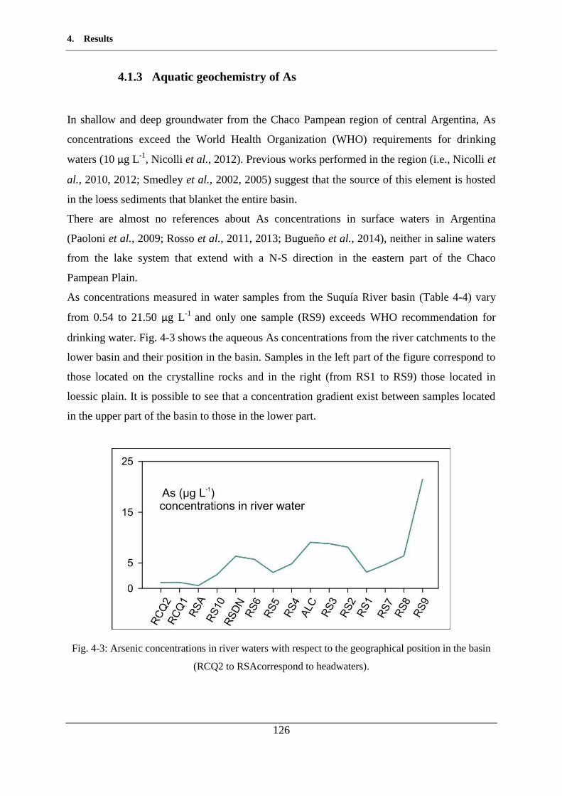
4. Results
126
4.1.3 Aquatic geochemistry of As
In shallow and deep groundwater from the Chaco Pampean region of central Argentina, As
concentrations exceed the World Health Organization (WHO) requirements for drinking
waters (10 µg L-1, Nicolli et al., 2012). Previous works performed in the region (i.e., Nicolli et
al., 2010, 2012; Smedley et al., 2002, 2005) suggest that the source of this element is hosted
in the loess sediments that blanket the entire basin.
There are almost no references about As concentrations in surface waters in Argentina
(Paoloni et al., 2009; Rosso et al., 2011, 2013; Bugueño et al., 2014), neither in saline waters
from the lake system that extend with a N-S direction in the eastern part of the Chaco
Pampean Plain.
As concentrations measured in water samples from the Suquía River basin (Table 4-4) vary
from 0.54 to 21.50 µg L-1 and only one sample (RS9) exceeds WHO recommendation for
drinking water. Fig. 4-3 shows the aqueous As concentrations from the river catchments to the
lower basin and their position in the basin. Samples in the left part of the figure correspond to
those located on the crystalline rocks and in the right (from RS1 to RS9) those located in
loessic plain. It is possible to see that a concentration gradient exist between samples located
in the upper part of the basin to those in the lower part.
Fig. 4-3: Arsenic concentrations in river waters with respect to the geographical position in the basin
(RCQ2 to RSAcorrespond to headwaters).
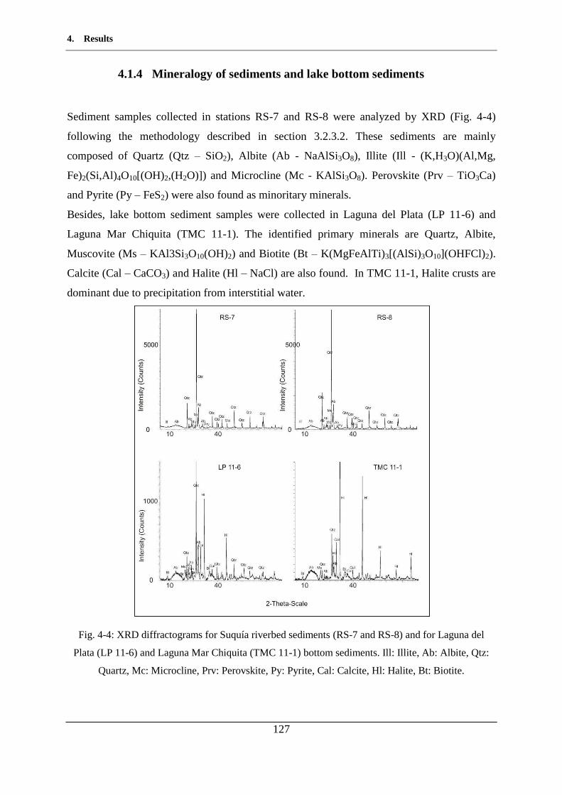
4. Results
127
4.1.4 Mineralogy of sediments and lake bottom sediments
Sediment samples collected in stations RS-7 and RS-8 were analyzed by XRD (Fig. 4-4)
following the methodology described in section 3.2.3.2. These sediments are mainly
composed of Quartz (Qtz – SiO2), Albite (Ab - NaAlSi3O8), Illite (Ill - (K,H 3O)(Al,Mg,
Fe)2(Si,Al)4O10[(OH)2,(H2O)]) and Microcline (Mc - KAlSi3O8). Perovskite (Prv – TiO3Ca)
and Pyrite (Py – FeS2) were also found as minoritary minerals.
Besides, lake bottom sediment samples were collected in Laguna del Plata (LP 11-6) and
Laguna Mar Chiquita (TMC 11-1). The identified primary minerals are Quartz, Albite,
Muscovite (Ms – KAl3Si3O10(OH)2) and Biotite (Bt – K(MgFeAlTi)3[(AlSi) 3O10](OHFCl)2).
Calcite (Cal – CaCO3) and Halite (Hl – NaCl) are also found. In TMC 11-1, Halite crusts are
dominant due to precipitation from interstitial water.
Fig. 4-4: XRD diffractograms for Suquía riverbed sediments (RS-7 and RS-8) and for Laguna del
Plata (LP 11-6) and Laguna Mar Chiquita (TMC 11-1) bottom sediments. Ill: Illite, Ab: Albite, Qtz:
Quartz, Mc: Microcline, Prv: Perovskite, Py: Pyrite, Cal: Calcite, Hl: Halite, Bt: Biotite.
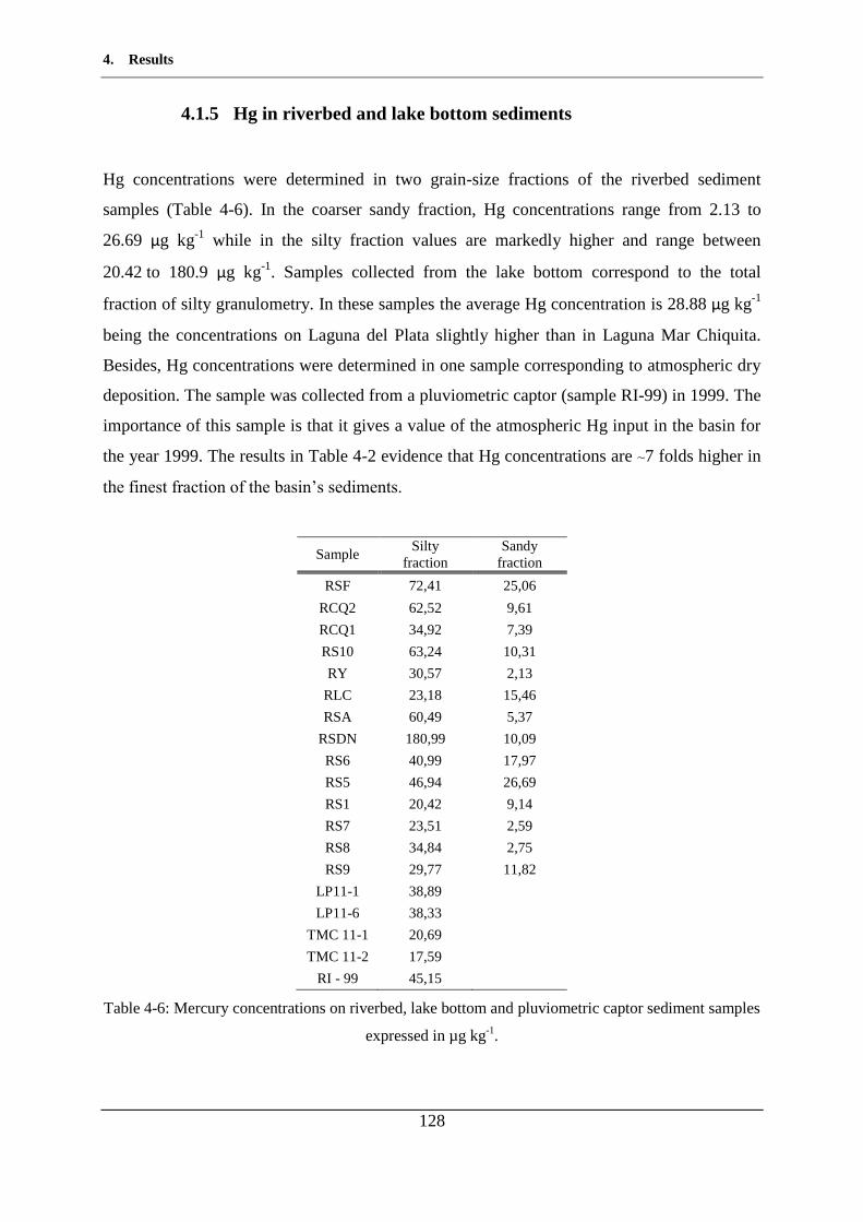
4. Results
128
4.1.5 Hg in riverbed and lake bottom sediments
Hg concentrations were determined in two grain-size fractions of the riverbed sediment
samples (Table 4-6). In the coarser sandy fraction, Hg concentrations range from 2.13 to
26.69 µg kg-1 while in the silty fraction values are markedly higher and range between
20.42 to 180.9 µg kg-1. Samples collected from the lake bottom correspond to the total
fraction of silty granulometry. In these samples the average Hg concentration is 28.88 µg kg-1
being the concentrations on Laguna del Plata slightly higher than in Laguna Mar Chiquita.
Besides, Hg concentrations were determined in one sample corresponding to atmospheric dry
deposition. The sample was collected from a pluviometric captor (sample RI-99) in 1999. The
importance of this sample is that it gives a value of the atmospheric Hg input in the basin for
the year 1999. The results in Table 4-2 evidence that Hg concentrations are ~7 folds higher in
the finest fraction of the basin’s sediments.
Sample Silty
fraction Sandy
fraction
RSF 72,41 25,06
RCQ2 62,52 9,61
RCQ1 34,92 7,39
RS10 63,24 10,31
RY 30,57 2,13
RLC 23,18 15,46
RSA 60,49 5,37
RSDN 180,99 10,09
RS6 40,99 17,97
RS5 46,94 26,69
RS1 20,42 9,14
RS7 23,51 2,59
RS8 34,84 2,75
RS9 29,77 11,82
LP11-1 38,89
LP11-6 38,33
TMC 11-1 20,69
TMC 11-2 17,59
RI - 99 45,15
Table 4-6: Mercury concentrations on riverbed, lake bottom and pluviometric captor sediment samples
expressed in µg kg-1.
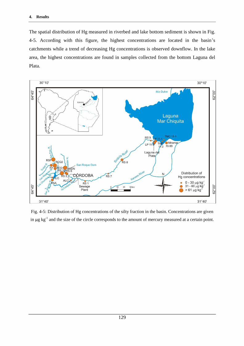
4. Results
129
The spatial distribution of Hg measured in riverbed and lake bottom sediment is shown in Fig.
4-5. According with this figure, the highest concentrations are located in the basin’s
catchments while a trend of decreasing Hg concentrations is observed downflow. In the lake
area, the highest concentrations are found in samples collected from the bottom Laguna del
Plata.
Fig. 4-5: Distribution of Hg concentrations of the silty fraction in the basin. Concentrations are given
in µg kg-1 and the size of the circle corresponds to the amount of mercury measured at a certain point.
4. Results
130
4.2 Geochemical and sedimentological characterization of the
sedimentary record in Laguna del Plata
A geo-physicochemical analysis of sediments of the LP core was carried out for the 120 cm
sedimentary core. Emphasis was made on Hg and As to understand the carrying phases that
these elements are associated to and their behaviour in the basin. These carrying phases were
analyzed through selective extractions following the methodology described in section 3.2.2.
In the obtained leachates, concentrations of Hg, As, Fe and Mn, were determined.
4.2.1 Textural, physical and chemical properties of the sediments
4.2.1.1 LP core sedimentation – Lamination Indexes
The description performed to the LP core was based on the Lamination Indexes (LI) proposed
by Piovano et al. (2002). These indexes are:
- Continuous laminae: when the layer is up to 2 mm thick are designated by “1”;
- Diffuse or discontinuous laminae: 2-4 mm thick by “2”;
- Thin banded: 4-10 mm thick by “3” ;
- Thick banded: >10 mm thick by “4”;
- Massive: when there is an absence of lamination.
LP core is characterised by an alternance of dark and light lamination which corresponds to
greyscale in the SCOPIX X-ray image and olive green scale colour in the photograph (Fig.
4-6a and b). Using these criteria 5 sedimentary units were recognised (Fig. 4-6).
The first one (A) is a massive sequence that extends from the bottom of the core up to 75 cm
with a net contact. From the base of the core to the top, this sequence shows different colours
on the photograph: light green colour in the deepest part, followed by a dark green olive
colour that overlies and a very light green colour on the top of it. In the X-Ray image the
colour varies from light gray in the bottom to darker gray in the upper part.
From 75 to 69 cm, it is possible to observe a group of LI2 (B) that is present as an alternance
of numerous dark to light colours layers with net contacts between them.
4. Results
131
Overlying this small sequence and up to 53 cm there is a group of sedimentary layers (C) that
correspond to LI4 that mix with LI2 in the base of the sequence, they show a predominance of
a light colour. The intercalations of the LI2 layers are net while the LI4 are quite diffuse or
gradual.
From here up to 16 cm a very regular sequence of LI1 and LI2 laminations (D) is present
intercalated with a LI3 lamination located between 27-39 cm the contacts between the thinner
layers are more net that those corresponding to the thicker ones.
The last 16 cm of the upper part of the core show a LI4 sequence (E) with dark olive green
colour in the picture and medium to light grey colour in the X-ray image. In the SCOPIX
image, the last 8 cm show a deformation of the sedimentary layers that could also be seen
between 58 and 60 cm, this is due to the opening of the core where the sediments moved at
the moment of separating both halves.
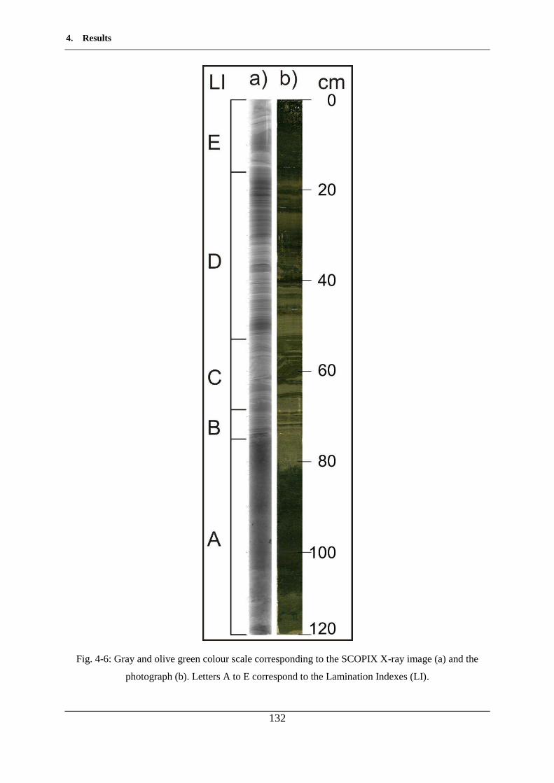
4. Results
132
Fig. 4-6: Gray and olive green colour scale corresponding to the SCOPIX X-ray image (a) and the
photograph (b). Letters A to E correspond to the Lamination Indexes (LI).
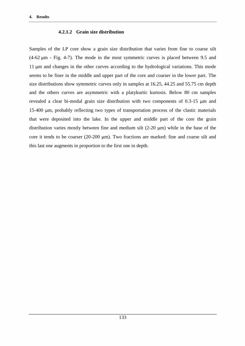
4. Results
133
4.2.1.2 Grain size distribution
Samples of the LP core show a grain size distribution that varies from fine to coarse silt
(4-62 µm - Fig. 4-7). The mode in the most symmetric curves is placed between 9.5 and
11 µm and changes in the other curves according to the hydrological variations. This mode
seems to be finer in the middle and upper part of the core and coarser in the lower part. The
size distributions show symmetric curves only in samples at 16.25, 44.25 and 55.75 cm depth
and the others curves are asymmetric with a platykurtic kurtosis. Below 80 cm samples
revealed a clear bi-modal grain size distribution with two components of 0.3-15 µm and
15-400 µm, probably reflecting two types of transportation process of the clastic materials
that were deposited into the lake. In the upper and middle part of the core the grain
distribution varies mostly between fine and medium silt (2-20 µm) while in the base of the
core it tends to be coarser (20-200 µm). Two fractions are marked: fine and coarse silt and
this last one augments in proportion to the first one in depth.
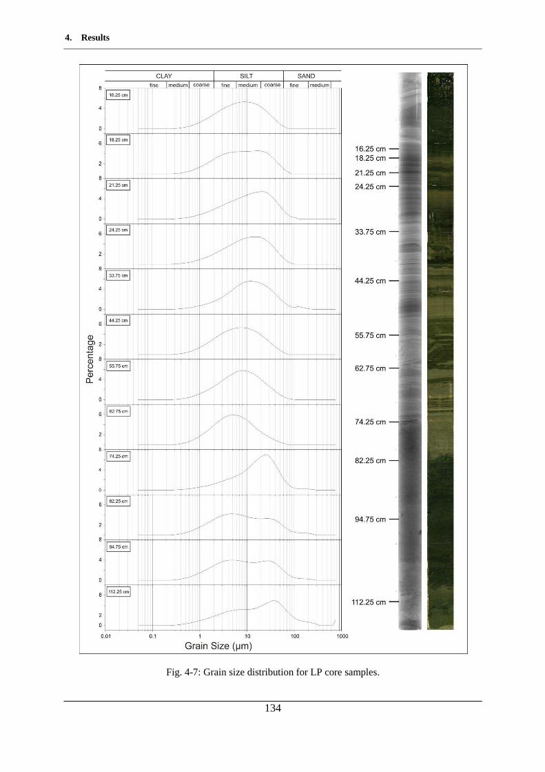
4. Results
134
Fig. 4-7: Grain size distribution for LP core samples.

4. Results
135
4.2.2 Physicochemical properties
Values of pH showe two different tendencies (Fig. 4-8d): from the bottom of the core up to
65.75 cm, the average is 9.20 while from this level up to the top measures show lower values
with an average of 8.51. The lower part corresponds to the period where the lake had low
lake-levels (Fig. 4-8c), high salinity and therefore higher pH. The opposite occurs in the upper
part of the core: when the lake-level started to rise, a marked diminution on the pH is
registered.
Porosity values ranged from 40.0 to 74.5 % (Fig. 4-8e). The lower values occurred near the
bottom of the LP core and the higher near the top. These allowed to divide the core into three
zones that are delimited in gray dashed lines in Fig. 4-8. In the first zone, that extends from
the bottom of the core to 74 cm, the porosity presented average values of 48.4 ± 2.9 %, in the
second one (from 74 to 16 cm) porosity raised up to 56.2 ± 6.1 % remaining nearly constant
and finally the upper zone that comprises the first 16 cm is represented by an abrupt
augmentation of water percentage (from 59.9 to 74.5 %). When regarding the core
sedimentation, it is possible to observe a relation with the lamination sections (Fig. 4-6) and
the porosity values, where section A corresponds to the lower porosity, B, C and D to the
intermediate porosity and E with the highest one.
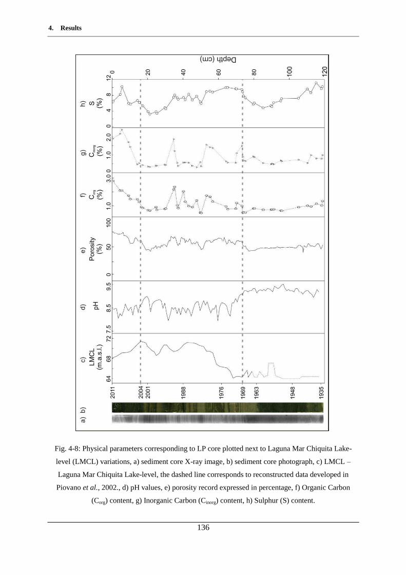
4. Results
136
Fig. 4-8: Physical parameters corresponding to LP core plotted next to Laguna Mar Chiquita Lake-
level (LMCL) variations, a) sediment core X-ray image, b) sediment core photograph, c) LMCL –
Laguna Mar Chiquita Lake-level, the dashed line corresponds to reconstructed data developed in
Piovano et al., 2002., d) pH values, e) porosity record expressed in percentage, f) Organic Carbon
(Corg) content, g) Inorganic Carbon (Cinorg) content, h) Sulphur (S) content.
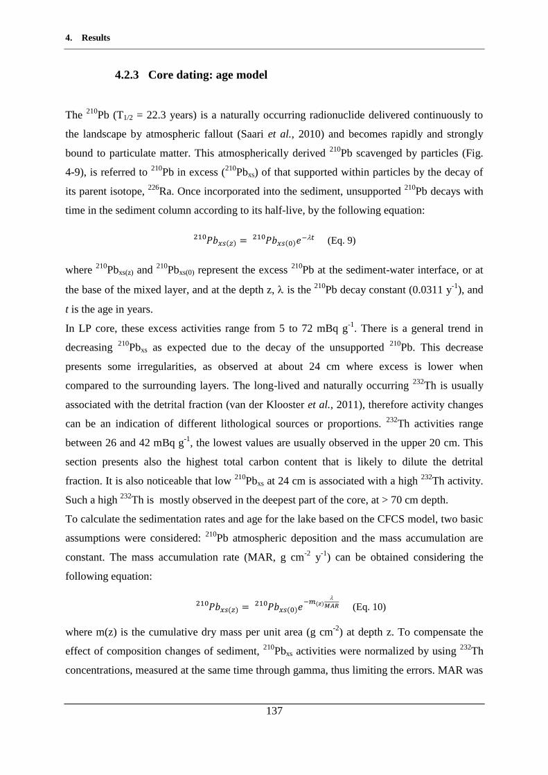
4. Results
137
4.2.3 Core dating: age model
The 210Pb (T1/2 = 22.3 years) is a naturally occurring radionuclide delivered continuously to
the landscape by atmospheric fallout (Saari et al., 2010) and becomes rapidly and strongly
bound to particulate matter. This atmospherically derived 210Pb scavenged by particles (Fig.
4-9), is referred to 210Pb in excess (210Pbxs) of that supported within particles by the decay of
its parent isotope, 226Ra. Once incorporated into the sediment, unsupported 210Pb decays with
time in the sediment column according to its half-live, by the following equation: (Eq. 9)
where 210Pbxs(z) and 210Pbxs(0) represent the excess 210Pb at the sediment-water interface, or at
the base of the mixed layer, and at the depth z, is the 210Pb decay constant (0.0311 y-1), and
t is the age in years.
In LP core, these excess activities range from 5 to 72 mBq g-1. There is a general trend in
decreasing 210Pbxs as expected due to the decay of the unsupported 210Pb. This decrease
presents some irregularities, as observed at about 24 cm where excess is lower when
compared to the surrounding layers. The long-lived and naturally occurring 232Th is usually
associated with the detrital fraction (van der Klooster et al., 2011), therefore activity changes
can be an indication of different lithological sources or proportions. 232Th activities range
between 26 and 42 mBq g-1, the lowest values are usually observed in the upper 20 cm. This
section presents also the highest total carbon content that is likely to dilute the detrital
fraction. It is also noticeable that low 210Pbxs at 24 cm is associated with a high 232Th activity.
Such a high 232Th is mostly observed in the deepest part of the core, at > 70 cm depth.
To calculate the sedimentation rates and age for the lake based on the CFCS model, two basic
assumptions were considered: 210Pb atmospheric deposition and the mass accumulation are
constant. The mass accumulation rate (MAR, g cm-2 y-1) can be obtained considering the
following equation:
(Eq. 10)
where m(z) is the cumulative dry mass per unit area (g cm-2) at depth z. To compensate the
effect of composition changes of sediment, 210Pbxs activities were normalized by using 232Th
concentrations, measured at the same time through gamma, thus limiting the errors. MAR was
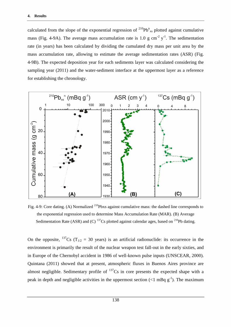
4. Results
138
calculated from the slope of the exponential regression of 210Pbnxs plotted against cumulative
mass (Fig. 4-9A). The average mass accumulation rate is 1.0 g cm-2 y-1. The sedimentation
rate (in years) has been calculated by dividing the cumulated dry mass per unit area by the
mass accumulation rate, allowing to estimate the average sedimentation rates (ASR) (Fig.
4-9B). The expected deposition year for each sediments layer was calculated considering the
sampling year (2011) and the water-sediment interface at the uppermost layer as a reference
for establishing the chronology.
Fig. 4-9: Core dating. (A) Normalized 210Pbxs against cumulative mass: the dashed line corresponds to
the exponential regression used to determine Mass Accumulation Rate (MAR). (B) Average
Sedimentation Rate (ASR) and (C) 137Cs plotted against calendar ages, based on 210Pb dating.
On the opposite, 137Cs (T1/2 = 30 years) is an artificial radionuclide: its occurrence in the
environment is primarily the result of the nuclear weapon test fall-out in the early sixties, and
in Europe of the Chernobyl accident in 1986 of well-known pulse inputs (UNSCEAR, 2000).
Quintana (2011) showed that at present, atmospheric fluxes in Buenos Aires province are
almost negligible. Sedimentary profile of 137Cs in core presents the expected shape with a
peak in depth and negligible activities in the uppermost section (<1 mBq g-1). The maximum
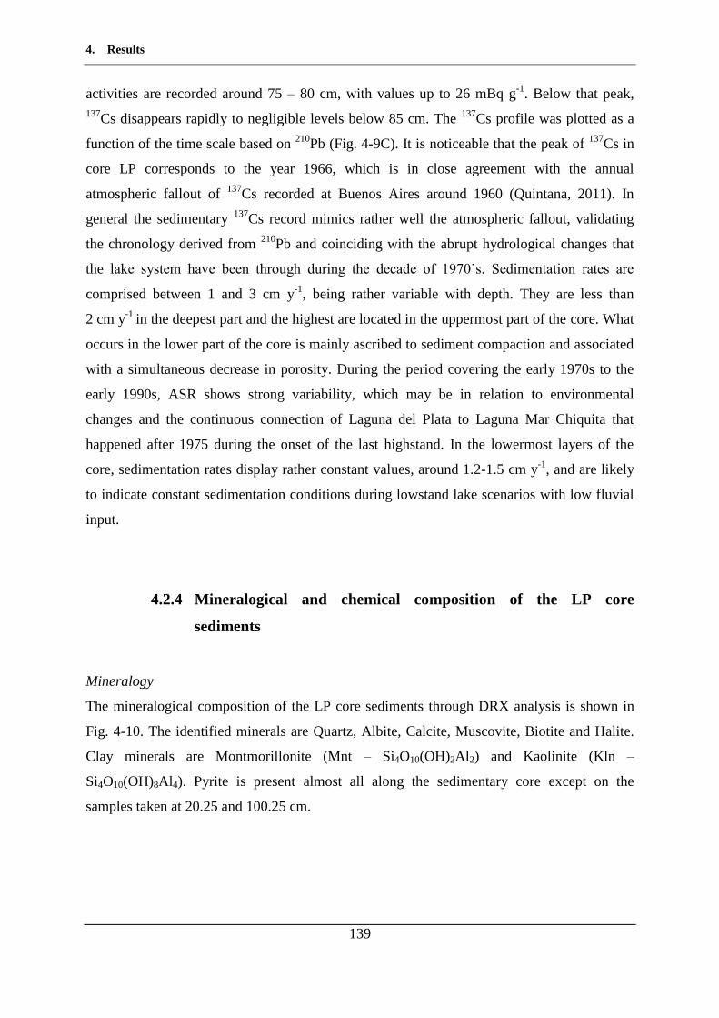
4. Results
139
activities are recorded around 75 – 80 cm, with values up to 26 mBq g-1. Below that peak, 137Cs disappears rapidly to negligible levels below 85 cm. The 137Cs profile was plotted as a
function of the time scale based on 210Pb (Fig. 4-9C). It is noticeable that the peak of 137Cs in
core LP corresponds to the year 1966, which is in close agreement with the annual
atmospheric fallout of 137Cs recorded at Buenos Aires around 1960 (Quintana, 2011). In
general the sedimentary 137Cs record mimics rather well the atmospheric fallout, validating
the chronology derived from 210Pb and coinciding with the abrupt hydrological changes that
the lake system have been through during the decade of 1970’s. Sedimentation rates are
comprised between 1 and 3 cm y-1, being rather variable with depth. They are less than
2 cm y-1 in the deepest part and the highest are located in the uppermost part of the core. What
occurs in the lower part of the core is mainly ascribed to sediment compaction and associated
with a simultaneous decrease in porosity. During the period covering the early 1970s to the
early 1990s, ASR shows strong variability, which may be in relation to environmental
changes and the continuous connection of Laguna del Plata to Laguna Mar Chiquita that
happened after 1975 during the onset of the last highstand. In the lowermost layers of the
core, sedimentation rates display rather constant values, around 1.2-1.5 cm y-1, and are likely
to indicate constant sedimentation conditions during lowstand lake scenarios with low fluvial
input.
4.2.4 Mineralogical and chemical composition of the LP core
sediments
Mineralogy
The mineralogical composition of the LP core sediments through DRX analysis is shown in
Fig. 4-10. The identified minerals are Quartz, Albite, Calcite, Muscovite, Biotite and Halite.
Clay minerals are Montmorillonite (Mnt – Si4O10(OH)2Al 2) and Kaolinite (Kln –
Si4O10(OH)8Al4). Pyrite is present almost all along the sedimentary core except on the
samples taken at 20.25 and 100.25 cm.
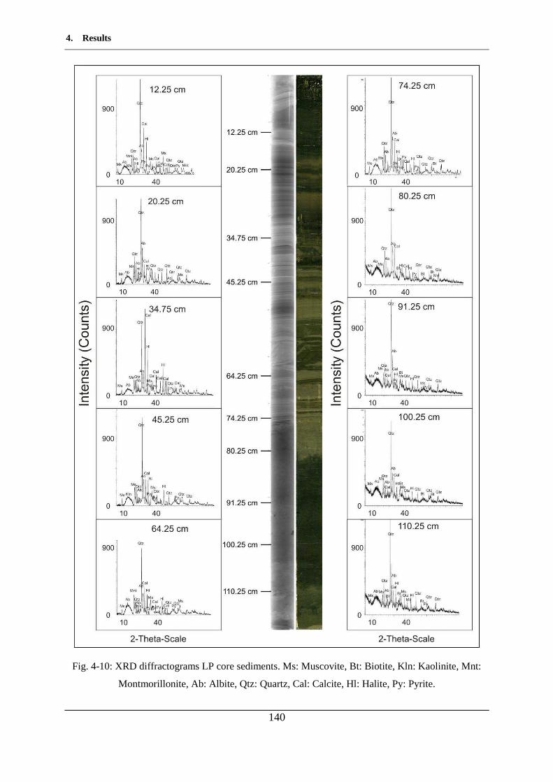
4. Results
140
Fig. 4-10: XRD diffractograms LP core sediments. Ms: Muscovite, Bt: Biotite, Kln: Kaolinite, Mnt:
Montmorillonite, Ab: Albite, Qtz: Quartz, Cal: Calcite, Hl: Halite, Py: Pyrite.
4. Results
141
Chemical composition
Organic carbon (Corg) values ranged between 0.49 and 2.79 % and those of inorganic carbon
(Cinorg) vary from 0.29 to 2.39 %. Regarding Corg (Fig. 4-8f), values remained almost constant
from 120 to 74 cm (0.83 % ± 0.22), while they show big fluctuations (between 0.49 to
2.36 %) from 74 up to 30 cm depth that are synchronous with porosity variations. The
uppermost centimetres present the highest values reaching a maximum of 2.79 % in the top of
the core. Cinorg variations are similar to those corresponding to Corg. From 120 to 74 cm its
average is 0.69 ± 0.17 %, from 74 to 16 cm it is 0.72 ± 0.46 % and in the last 16 cm the
average value is 1.51 ± 0.76 % (Fig. 4-8g). Cinorg represents the contents of carbonates in the
sediments, which range from 2.42 to 19.91 % along the LP core. Carbonate values in Laguna
Mar Chiquita span a wider range of concentrations, varying between 0.4 and 25.0 %.
Sulphur (S) concentrations along the sedimentary core oscillate between 3.2 and 11.2 %. The
profile shown in Fig. 4-8h evidences three zones in where the maximum S values are
registered: underneath 100 cm, between 74 and 35 cm and above 16 cm. These concentrations
are assigned to the presence of disseminated sulphides and sulphates along the core. S seems
to well correlate with Cinorg in the lower part of the core and in the uppermost part, while in
the middle part (from 74 to 16 cm) it better correlates with Corg. Gypsum is a very common
mineral found in sediment cores of the neighbouring Laguna Mar Chiquita (Piovano et al.,
2002; Bucher and Bucher, 2006a) especially when the lake presents low lake-levels, but it has
not been detected by XRD analysis performed in the LP core.
The contents of some other elements were determined through the core by XRF, depicting
mainly three domains (Fig. 4-11). The lower part of the core from the base up to 74 cm is
characterised by a signal that remains almost constant except for Zr, S, Sr and Ca that rises in
the last centimetres. The second domain shows a high fluctuation visible in all the measured
elements that extends in the central part of the core up to 16 cm. From here up to the top Al,
Si, K, Ti, Mn, Fe and Zr show a diminution in the signal while for Sr, S, Cl and Ca the
opposite occurs.
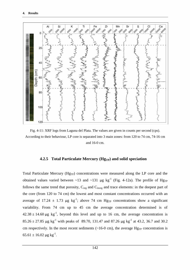
4. Results
142
Fig. 4-11: XRF logs from Laguna del Plata. The values are given in counts per second (cps).
According to their behaviour, LP core is separated into 3 main zones: from 120 to 74 cm, 74-16 cm
and 16-0 cm.
4.2.5 Total Particulate Mercury (Hg TP) and solid speciation
Total Particulate Mercury (HgTP) concentrations were measured along the LP core and the
obtained values varied between ~13 and ~131 µg kg-1 (Fig. 4-12a). The profile of HgTP
follows the same trend that porosity, Corg and Cinorg and trace elements: in the deepest part of
the core (from 120 to 74 cm) the lowest and most constant concentrations occurred with an
average of 17.24 ± 1.73 µg kg-1; above 74 cm HgTP concentrations show a significant
variability. From 74 cm up to 45 cm the average concentration determined is of
42.38 ± 14.60 µg kg-1, beyond this level and up to 16 cm, the average concentration is
85.26 ± 27.85 µg kg-1 with peaks of 89.70, 131.47 and 87.26 µg kg-1 at 43.2, 36.7 and 30.2
cm respectively. In the most recent sediments (~16-0 cm), the average HgTP concentration is
65.61 ± 16.02 µg kg-1.
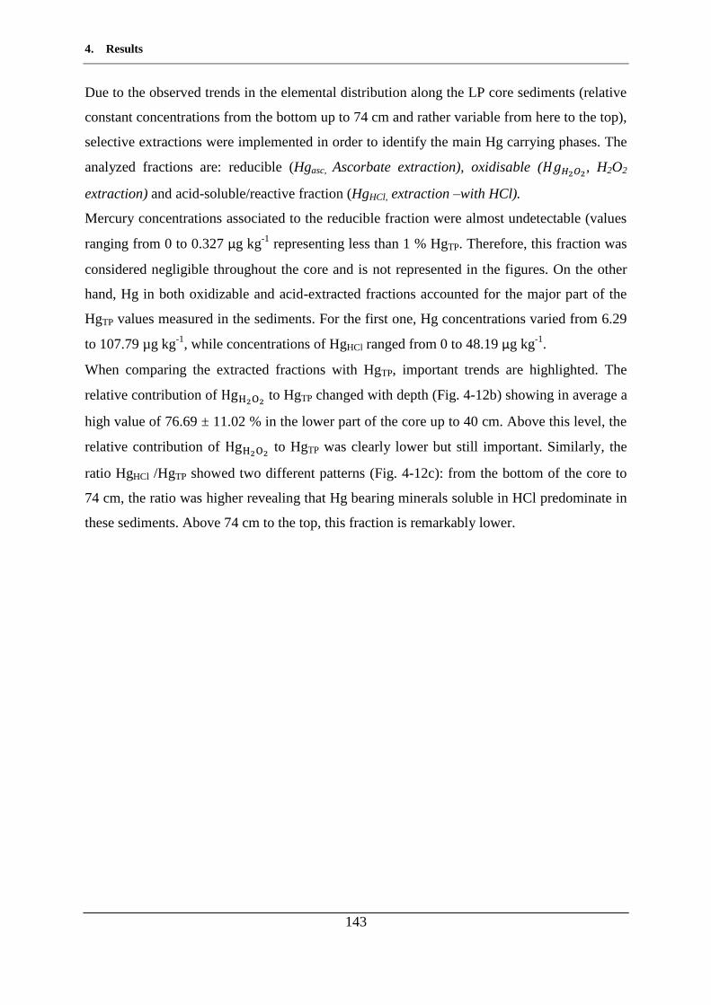
4. Results
143
Due to the observed trends in the elemental distribution along the LP core sediments (relative
constant concentrations from the bottom up to 74 cm and rather variable from here to the top),
selective extractions were implemented in order to identify the main Hg carrying phases. The
analyzed fractions are: reducible (Hgasc, Ascorbate extraction), oxidisable ( , H2O2
extraction) and acid-soluble/reactive fraction (HgHCl, extraction –with HCl).
Mercury concentrations associated to the reducible fraction were almost undetectable (values
ranging from 0 to 0.327 µg kg-1 representing less than 1 % HgTP. Therefore, this fraction was
considered negligible throughout the core and is not represented in the figures. On the other
hand, Hg in both oxidizable and acid-extracted fractions accounted for the major part of the
HgTP values measured in the sediments. For the first one, Hg concentrations varied from 6.29
to 107.79 µg kg-1, while concentrations of HgHCl ranged from 0 to 48.19 µg kg-1.
When comparing the extracted fractions with HgTP, important trends are highlighted. The
relative contribution of to HgTP changed with depth (Fig. 4-12b) showing in average a
high value of 76.69 ± 11.02 % in the lower part of the core up to 40 cm. Above this level, the
relative contribution of to HgTP was clearly lower but still important. Similarly, the
ratio HgHCl /HgTP showed two different patterns (Fig. 4-12c): from the bottom of the core to
74 cm, the ratio was higher revealing that Hg bearing minerals soluble in HCl predominate in
these sediments. Above 74 cm to the top, this fraction is remarkably lower.
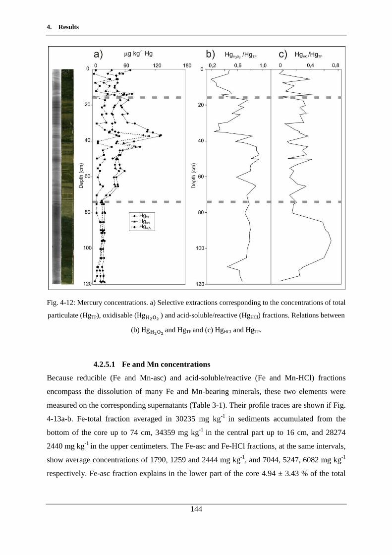
4. Results
144
Fig. 4-12: Mercury concentrations. a) Selective extractions corresponding to the concentrations of total
particulate (HgTP), oxidisable ( ) and acid-soluble/reactive (HgHCl) fractions. Relations between
(b) and HgTP and (c) HgHCl and HgTP.
4.2.5.1 Fe and Mn concentrations
Because reducible (Fe and Mn-asc) and acid-soluble/reactive (Fe and Mn-HCl) fractions
encompass the dissolution of many Fe and Mn-bearing minerals, these two elements were
measured on the corresponding supernatants (Table 3-1). Their profile traces are shown if Fig.
4-13a-b. Fe-total fraction averaged in 30235 mg kg-1 in sediments accumulated from the
bottom of the core up to 74 cm, 34359 mg kg-1 in the central part up to 16 cm, and 28274
2440 mg kg-1 in the upper centimeters. The Fe-asc and Fe-HCl fractions, at the same intervals,
show average concentrations of 1790, 1259 and 2444 mg kg-1, and 7044, 5247, 6082 mg kg-1
respectively. Fe-asc fraction explains in the lower part of the core 4.94 ± 3.43 % of the total
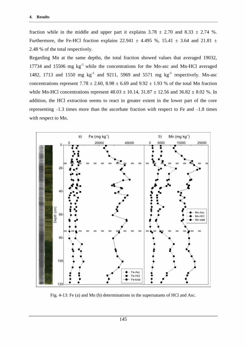
4. Results
145
fraction while in the middle and upper part it explains 3.78 ± 2.70 and 8.33 ± 2.74 %.
Furthermore, the Fe-HCl fraction explains 22.941 ± 4.495 %, 15.41 ± 3.64 and 21.81 ±
2.48 % of the total respectively.
Regarding Mn at the same depths, the total fraction showed values that averaged 19032,
17734 and 15506 mg kg-1 while the concentrations for the Mn-asc and Mn-HCl averaged
1482, 1713 and 1550 mg kg-1 and 9211, 5969 and 5571 mg kg-1 respectively. Mn-asc
concentrations represent 7.78 ± 2.60, 8.98 ± 6.69 and 9.92 ± 1.93 % of the total Mn fraction
while Mn-HCl concentrations represent 48.03 ± 10.14, 31.87 ± 12.56 and 36.82 ± 8.02 %. In
addition, the HCl extraction seems to react in greater extent in the lower part of the core
representing ~1.3 times more than the ascorbate fraction with respect to Fe and ~1.8 times
with respect to Mn.
Fig. 4-13: Fe (a) and Mn (b) determinations in the supernatants of HCl and Asc.
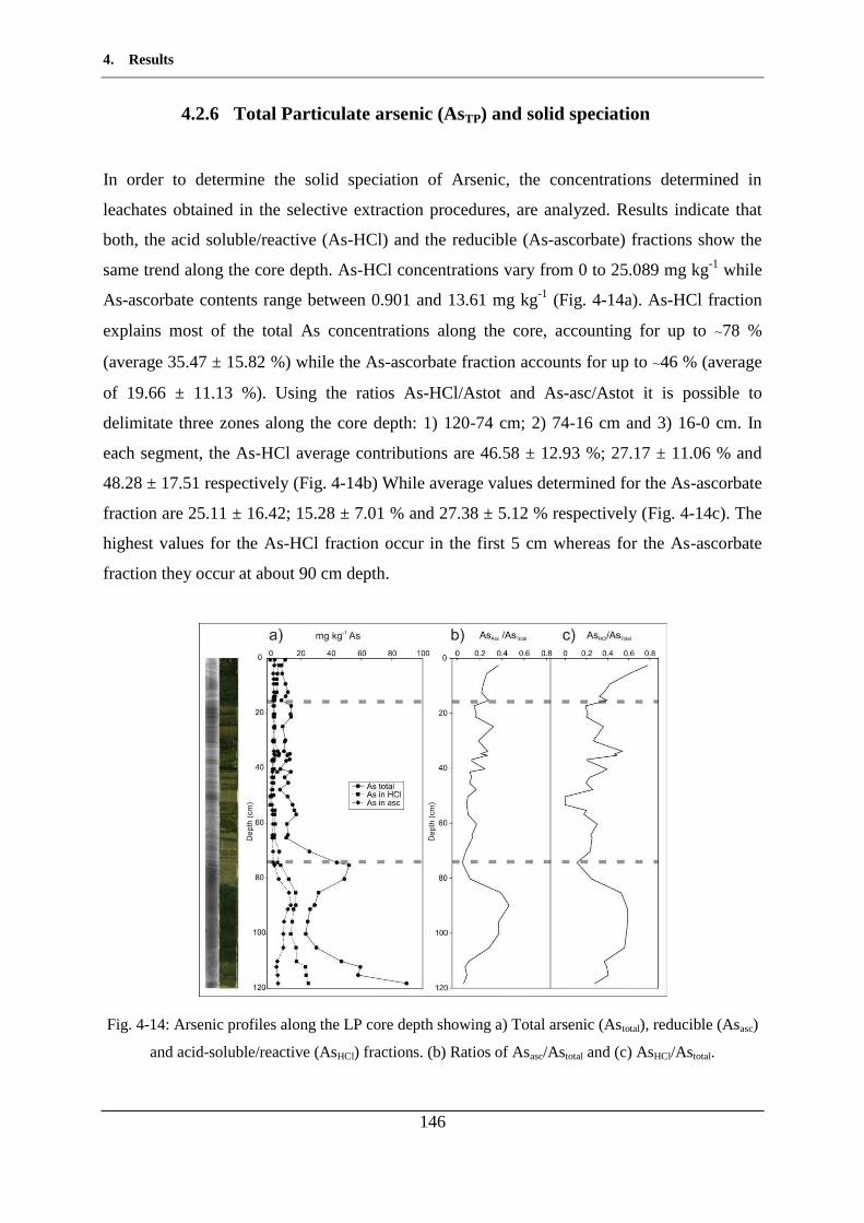
4. Results
146
4.2.6 Total Particulate arsenic (AsTP) and solid speciation
In order to determine the solid speciation of Arsenic, the concentrations determined in
leachates obtained in the selective extraction procedures, are analyzed. Results indicate that
both, the acid soluble/reactive (As-HCl) and the reducible (As-ascorbate) fractions show the
same trend along the core depth. As-HCl concentrations vary from 0 to 25.089 mg kg-1 while
As-ascorbate contents range between 0.901 and 13.61 mg kg-1 (Fig. 4-14a). As-HCl fraction
explains most of the total As concentrations along the core, accounting for up to ~78 %
(average 35.47 ± 15.82 %) while the As-ascorbate fraction accounts for up to ~46 % (average
of 19.66 ± 11.13 %). Using the ratios As-HCl/Astot and As-asc/Astot it is possible to
delimitate three zones along the core depth: 1) 120-74 cm; 2) 74-16 cm and 3) 16-0 cm. In
each segment, the As-HCl average contributions are 46.58 ± 12.93 %; 27.17 ± 11.06 % and
48.28 ± 17.51 respectively (Fig. 4-14b) While average values determined for the As-ascorbate
fraction are 25.11 ± 16.42; 15.28 ± 7.01 % and 27.38 ± 5.12 % respectively (Fig. 4-14c). The
highest values for the As-HCl fraction occur in the first 5 cm whereas for the As-ascorbate
fraction they occur at about 90 cm depth.
Fig. 4-14: Arsenic profiles along the LP core depth showing a) Total arsenic (Astotal), reducible (Asasc)
and acid-soluble/reactive (AsHCl) fractions. (b) Ratios of Asasc/Astotal and (c) AsHCl/Astotal.
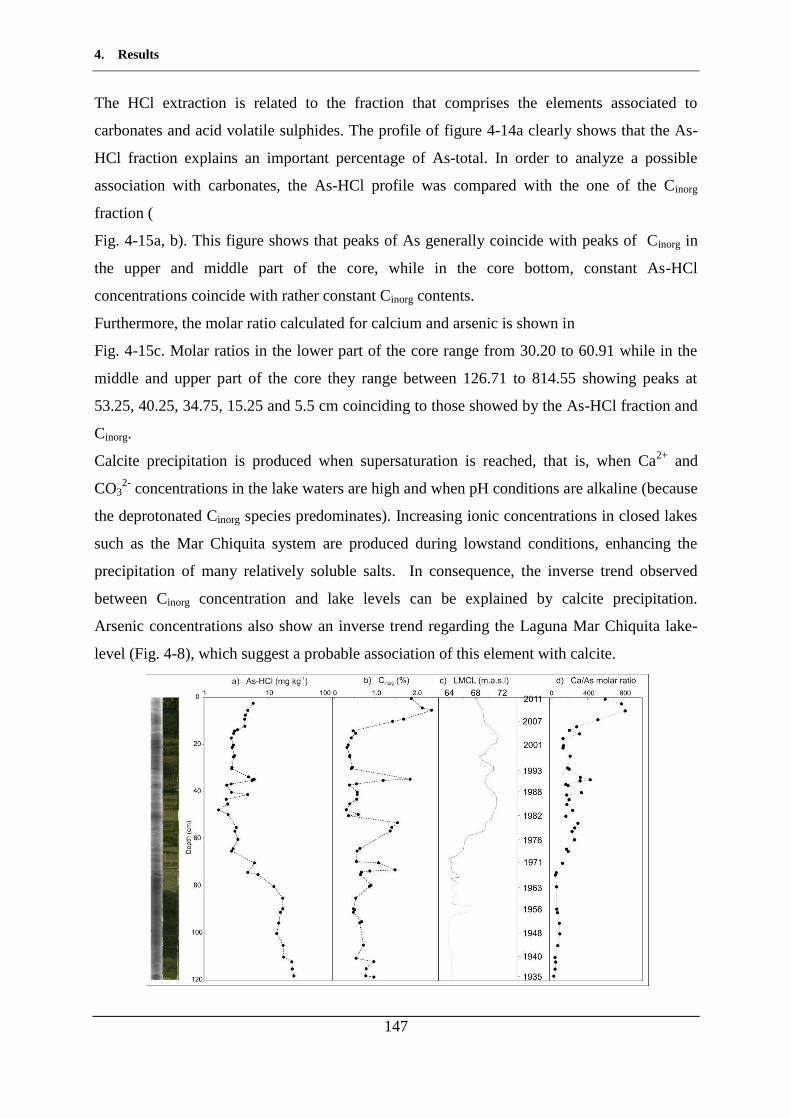
4. Results
147
The HCl extraction is related to the fraction that comprises the elements associated to
carbonates and acid volatile sulphides. The profile of figure 4-14a clearly shows that the As-
HCl fraction explains an important percentage of As-total. In order to analyze a possible
association with carbonates, the As-HCl profile was compared with the one of the Cinorg
fraction (
Fig. 4-15a, b). This figure shows that peaks of As generally coincide with peaks of Cinorg in
the upper and middle part of the core, while in the core bottom, constant As-HCl
concentrations coincide with rather constant Cinorg contents.
Furthermore, the molar ratio calculated for calcium and arsenic is shown in
Fig. 4-15c. Molar ratios in the lower part of the core range from 30.20 to 60.91 while in the
middle and upper part of the core they range between 126.71 to 814.55 showing peaks at
53.25, 40.25, 34.75, 15.25 and 5.5 cm coinciding to those showed by the As-HCl fraction and
Cinorg.
Calcite precipitation is produced when supersaturation is reached, that is, when Ca2+ and
CO32- concentrations in the lake waters are high and when pH conditions are alkaline (because
the deprotonated Cinorg species predominates). Increasing ionic concentrations in closed lakes
such as the Mar Chiquita system are produced during lowstand conditions, enhancing the
precipitation of many relatively soluble salts. In consequence, the inverse trend observed
between Cinorg concentration and lake levels can be explained by calcite precipitation.
Arsenic concentrations also show an inverse trend regarding the Laguna Mar Chiquita lake-
level (Fig. 4-8), which suggest a probable association of this element with calcite.
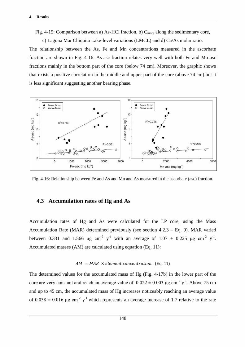
4. Results
148
Fig. 4-15: Comparison between a) As-HCl fraction, b) Cinorg along the sedimentary core,
c) Laguna Mar Chiquita Lake-level variations (LMCL) and d) Ca/As molar ratio.
The relationship between the As, Fe and Mn concentrations measured in the ascorbate
fraction are shown in Fig. 4-16. As-asc fraction relates very well with both Fe and Mn-asc
fractions mainly in the bottom part of the core (below 74 cm). Moreover, the graphic shows
that exists a positive correlation in the middle and upper part of the core (above 74 cm) but it
is less significant suggesting another bearing phase.
Fig. 4-16: Relationship between Fe and As and Mn and As measured in the ascorbate (asc) fraction.
4.3 Accumulation rates of Hg and As
Accumulation rates of Hg and As were calculated for the LP core, using the Mass
Accumulation Rate (MAR) determined previously (see section 4.2.3 – Eq. 9). MAR varied
between 0.331 and 1.566 μg cm-2 y-1 with an average of 1.07 ± 0.225 μg cm-2 y-1.
Accumulated masses (AM) are calculated using equation (Eq. 11):
(Eq. 11)
The determined values for the accumulated mass of Hg (Fig. 4-17b) in the lower part of the
core are very constant and reach an average value of 0.022 ˃ 0.003 μg cm-2 y-1. Above 75 cm
and up to 45 cm, the accumulated mass of Hg increases noticeably reaching an average value
of 0.038 ˃ 0.016 μg cm-2 y-1 which represents an average increase of 1.7 relative to the rate
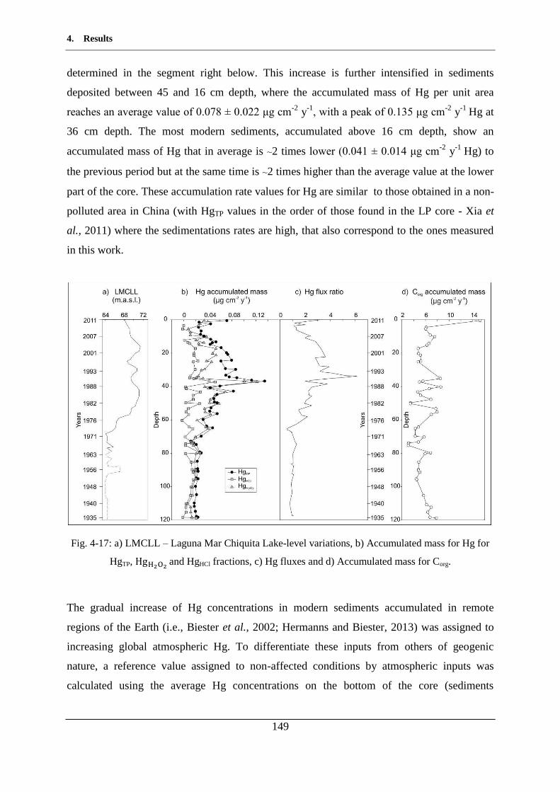
4. Results
149
determined in the segment right below. This increase is further intensified in sediments
deposited between 45 and 16 cm depth, where the accumulated mass of Hg per unit area
reaches an average value of 0.078 ˃ 0.022 μg cm-2 y-1, with a peak of 0.135 μg cm-2 y-1 Hg at
36 cm depth. The most modern sediments, accumulated above 16 cm depth, show an
accumulated mass of Hg that in average is ~2 times lower (0.041 ˃ 0.014 μg cm-2 y-1 Hg) to
the previous period but at the same time is ~2 times higher than the average value at the lower
part of the core. These accumulation rate values for Hg are similar to those obtained in a non-
polluted area in China (with HgTP values in the order of those found in the LP core - Xia et
al., 2011) where the sedimentations rates are high, that also correspond to the ones measured
in this work.
Fig. 4-17: a) LMCLL – Laguna Mar Chiquita Lake-level variations, b) Accumulated mass for Hg for
HgTP, and HgHCl fractions, c) Hg fluxes and d) Accumulated mass for Corg.
The gradual increase of Hg concentrations in modern sediments accumulated in remote
regions of the Earth (i.e., Biester et al., 2002; Hermanns and Biester, 2013) was assigned to
increasing global atmospheric Hg. To differentiate these inputs from others of geogenic
nature, a reference value assigned to non-affected conditions by atmospheric inputs was
calculated using the average Hg concentrations on the bottom of the core (sediments
4. Results
150
accumulated before 1970). This assumption is based on the constancy of the values registered
in this part of the core and the similitude of these values with those measured in sediments of
the Suquía River basin (Table 4-6), suggesting that these sediments could have been the main
source of Hg to the lake in the years prior to 1970. Fig. 4-17c shows the obtained profile of
the ratio between the accumulated mass of Hg and the corresponding background value. It is
possible to see a gradual increase in the accumulation rate of Hg from early 1970s, reaching
values ~3.5 times higher in sediments accumulated in the year 2011 with respect to those
registered in the sediments accumulated before 1970. Despite this marked increase, the
maximum accumulation values of Hg occurred between 1990 and 1995, when peaks between
~ 4 and ~ 7 times higher than the background values were registered.
When calculating the accumulated mass per unit area of the two extracted fractions of Hg, it
appears that much of the increase in the flux of Hg in sediments accumulated between 75 and
16 cm depth is explained mainly by the contribution of Hg associated with oxidizable fraction
(organic matter + sulphide). This fraction explains almost 100 % of the accumulated mass
until approximately the year 1990. In the most recent sediments there is an Hg excess that
cannot be explained by neither of both fractions (Fig. 4-17b).
Following the same procedure, the accumulated mass of organic carbon (Corg) was calculated
along the core. The obtained profile (Fig. 4-17d) shows a distribution more or less constant
from the bottom of the core until the 16 cm (average accumulated mass
5.55 ± 1.52 μg cm-2 y-1 C). Above this level, the accumulated mass of C starts to gradually
increase reaching an average value of 7.79 ˃ 3.57 μg cm-2 y-1 C. This distribution prompts that
the organic matter contribution was more or less constant between 1935 and 2003 and that the
beginning of the humid period from in the beginning of the 1970s only affected the variability
in the organic matter input to the lake, without significantly altering its average accumulated
mass. Consequently, increasing Hg associated to the oxidizable phase in the sediments
accumulated between 75 and 16 cm depth may be assigned not only to the organic matter but
also to the presence of other oxidizable phases in the sediment, probably pyrite since this
mineral has been identified through the analysis of X-ray diffraction (Fig. 4-10).
Beyond the predominance of the oxidizable fraction along the entire sedimentary core, the
bioavailable fraction also plays an important role in solid speciation of Hg, especially below
74 cm depth (Fig. 4-17b). This fraction represents the Hg that is adsorbed on the surface of Fe
and Mn oxides or other minerals, including pyrite.
4. Results
151
The distribution of the Fe and Mn concentrations measured in the ascorbate extraction
revealed a strong presence of oxides below 80 cm and above 40 cm (Fig. 4-13). Hg extracted
in this same fraction is negligible, suggesting that most of the Hg present at these levels is not
associated to Fe and Mn-oxide coatings. Accordingly most of the Hg extracted with HCl
would be associated to pyrite (total S oscillates between 5 to 10 % in these levels, Fig. 4-8).
As accumulation rates (Fig. 4-18a) were calculated using Eq. 10. In average, rates in the
bottom of the core up to 74 cm were 53.54 ± 24.77 μg cm-2 y-1 As while in the top core, the
calculated average value was 11.03 ± 4.42 μg cm-2 y-1 As. The accumulation rates determined
for the As–HCl and As-asc fractions show a clear predominance of the former. In the deeper
part of the core, average values for As-HCl fraction were 19.22 ˃ 6.99 μg cm-2 y-1 As against
8.88 ˃ 4.89 μg cm-2 y-1 corresponding to the accumulation rates of the As-asc fraction. In the
upper part of the core, the As-HCl fraction average an accumulation rate of
2.88 ± 1.28 μg cm-2 y-1 while the As-asc fraction, 1.91 ± 0.685 μg cm-2 y-1.
As previously indicated for Hg, As fluxes were calculated for sediments accumulated in the
LP core. Fig. 4-14a shows that the most constant values of As were measured in sediments
accumulated in the range of depth between 74 cm and the top of the core. The average
accumulated mass of AsTP for this section was 11.03 ± 4.42 μg cm-2 y-1. This value was used
as a reference of background conditions. As seen in the profile that shows the As
accumulation rates in depth (Fig. 4-18b), under dry conditions, the deposition of As-bearing
sediments was ~5 times higher than under humid conditions that prevailed from the beginning
of the 1970s. Besides, a marked peak is observed at 75 cm depth. After this period, As flux
show a decreasing pattern. The two analyzed As fractions follow a similar trend, but they
cannot explain the total As accumulation rate in the lower part of the core As-HCl counts in
average for 41.29 % and As-asc counts for 22.36 % of the total As. All along the lower
segment of the core, the As acid-soluble fraction (As-HCl) predominates over the reducible
fraction (As-asc), indicating that As is preferentially released from the sediments due to the
dissolution of some acid-soluble As-bearing mineral. Some As is also considered to be
adsorbed onto Fe and Mn hydr(oxides) in these sediments. In agreement, the Fe and Mn
profiles for the reducible fraction (Fig. 4-13) correlates with that of the As. The adsorption of
arsenate ions onto Fe (oxy)hydroxides occurs under neutral to acidic conditions; desorption,
hence, is favoured at alkaline pH (Hiemstra and Van Riemsdijk, 2000).
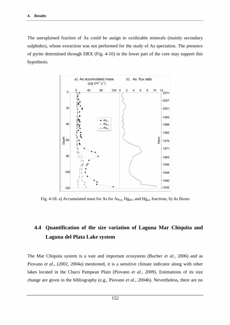
4. Results
152
The unexplained fraction of As could be assign to oxidizable minerals (mainly secondary
sulphides), whose extraction was not performed for the study of As speciation. The presence
of pyrite determined through DRX (Fig. 4-10) in the lower part of the core may support this
hypothesis.
Fig. 4-18: a) Accumulated mass for As for Astot, HgHCl and Hgasc fractions, b) As fluxes
4.4 Quantification of the size variation of Laguna Mar Chiquita and
Laguna del Plata Lake system
The Mar Chiquita system is a vast and important ecosystem (Bucher et al., 2006) and as
Piovano et al., (2002, 2004a) mentioned, it is a sensitive climate indicator along with other
lakes located in the Chaco Pampean Plain (Piovano et al., 2009). Estimations of its size
change are given in the bibliography (e.g., Piovano et al., 2004b). Nevertheless, there are no
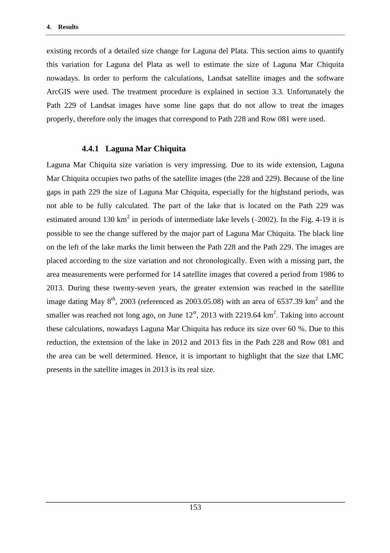
4. Results
153
existing records of a detailed size change for Laguna del Plata. This section aims to quantify
this variation for Laguna del Plata as well to estimate the size of Laguna Mar Chiquita
nowadays. In order to perform the calculations, Landsat satellite images and the software
ArcGIS were used. The treatment procedure is explained in section 3.3. Unfortunately the
Path 229 of Landsat images have some line gaps that do not allow to treat the images
properly, therefore only the images that correspond to Path 228 and Row 081 were used.
4.4.1 Laguna Mar Chiquita
Laguna Mar Chiquita size variation is very impressing. Due to its wide extension, Laguna
Mar Chiquita occupies two paths of the satellite images (the 228 and 229). Because of the line
gaps in path 229 the size of Laguna Mar Chiquita, especially for the highstand periods, was
not able to be fully calculated. The part of the lake that is located on the Path 229 was
estimated around 130 km2 in periods of intermediate lake levels (~2002). In the Fig. 4-19 it is
possible to see the change suffered by the major part of Laguna Mar Chiquita. The black line
on the left of the lake marks the limit between the Path 228 and the Path 229. The images are
placed according to the size variation and not chronologically. Even with a missing part, the
area measurements were performed for 14 satellite images that covered a period from 1986 to
2013. During these twenty-seven years, the greater extension was reached in the satellite
image dating May 8th, 2003 (referenced as 2003.05.08) with an area of 6537.39 km2 and the
smaller was reached not long ago, on June 12st, 2013 with 2219.64 km2. Taking into account
these calculations, nowadays Laguna Mar Chiquita has reduce its size over 60 %. Due to this
reduction, the extension of the lake in 2012 and 2013 fits in the Path 228 and Row 081 and
the area can be well determined. Hence, it is important to highlight that the size that LMC
presents in the satellite images in 2013 is its real size.
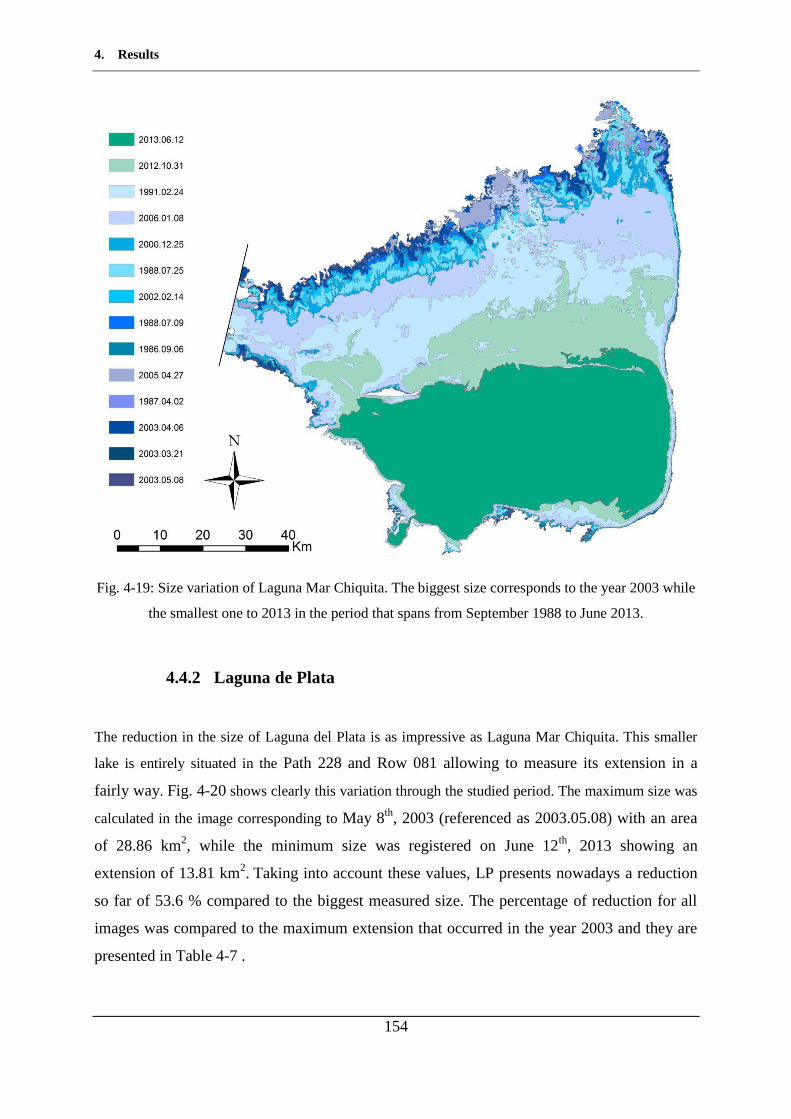
4. Results
154
Fig. 4-19: Size variation of Laguna Mar Chiquita. The biggest size corresponds to the year 2003 while
the smallest one to 2013 in the period that spans from September 1988 to June 2013.
4.4.2 Laguna de Plata
The reduction in the size of Laguna del Plata is as impressive as Laguna Mar Chiquita. This smaller
lake is entirely situated in the Path 228 and Row 081 allowing to measure its extension in a
fairly way. Fig. 4-20 shows clearly this variation through the studied period. The maximum size was
calculated in the image corresponding to May 8th, 2003 (referenced as 2003.05.08) with an area
of 28.86 km2, while the minimum size was registered on June 12th, 2013 showing an
extension of 13.81 km2. Taking into account these values, LP presents nowadays a reduction
so far of 53.6 % compared to the biggest measured size. The percentage of reduction for all
images was compared to the maximum extension that occurred in the year 2003 and they are
presented in Table 4-7 .
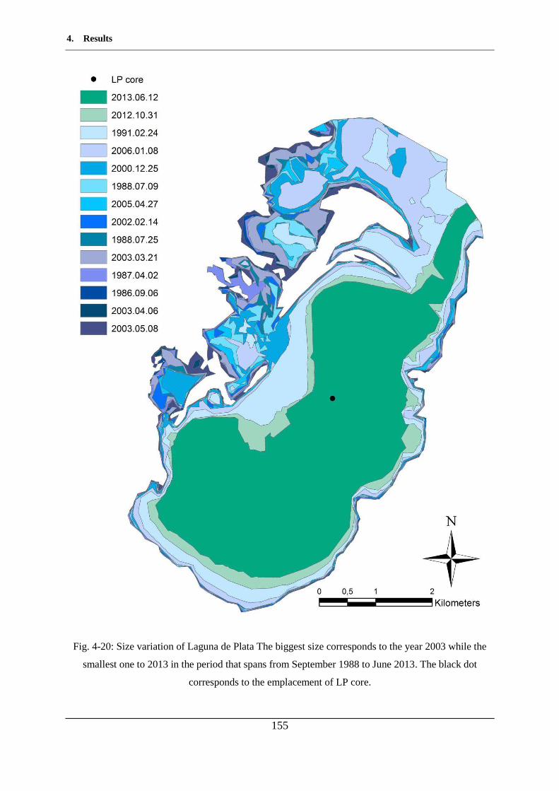
4. Results
155
Fig. 4-20: Size variation of Laguna de Plata The biggest size corresponds to the year 2003 while the
smallest one to 2013 in the period that spans from September 1988 to June 2013. The black dot
corresponds to the emplacement of LP core.
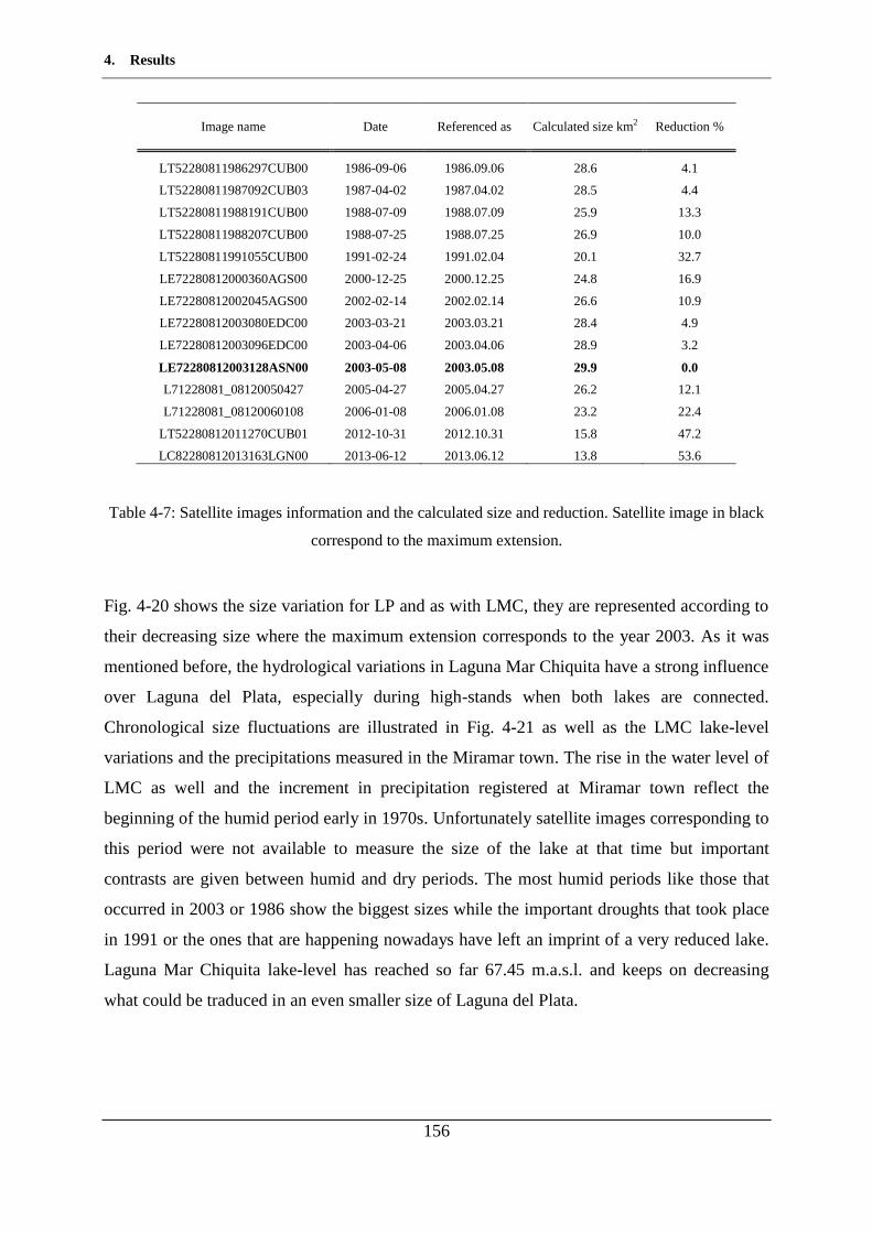
4. Results
156
Image name Date Referenced as Calculated size km2 Reduction %
LT52280811986297CUB00 1986-09-06 1986.09.06 28.6 4.1
LT52280811987092CUB03 1987-04-02 1987.04.02 28.5 4.4
LT52280811988191CUB00 1988-07-09 1988.07.09 25.9 13.3
LT52280811988207CUB00 1988-07-25 1988.07.25 26.9 10.0
LT52280811991055CUB00 1991-02-24 1991.02.04 20.1 32.7
LE72280812000360AGS00 2000-12-25 2000.12.25 24.8 16.9
LE72280812002045AGS00 2002-02-14 2002.02.14 26.6 10.9
LE72280812003080EDC00 2003-03-21 2003.03.21 28.4 4.9
LE72280812003096EDC00 2003-04-06 2003.04.06 28.9 3.2
LE72280812003128ASN00 2003-05-08 2003.05.08 29.9 0.0
L71228081_08120050427 2005-04-27 2005.04.27 26.2 12.1
L71228081_08120060108 2006-01-08 2006.01.08 23.2 22.4
LT52280812011270CUB01 2012-10-31 2012.10.31 15.8 47.2
LC82280812013163LGN00 2013-06-12 2013.06.12 13.8 53.6
Table 4-7: Satellite images information and the calculated size and reduction. Satellite image in black
correspond to the maximum extension.
Fig. 4-20 shows the size variation for LP and as with LMC, they are represented according to
their decreasing size where the maximum extension corresponds to the year 2003. As it was
mentioned before, the hydrological variations in Laguna Mar Chiquita have a strong influence
over Laguna del Plata, especially during high-stands when both lakes are connected.
Chronological size fluctuations are illustrated in Fig. 4-21 as well as the LMC lake-level
variations and the precipitations measured in the Miramar town. The rise in the water level of
LMC as well and the increment in precipitation registered at Miramar town reflect the
beginning of the humid period early in 1970s. Unfortunately satellite images corresponding to
this period were not available to measure the size of the lake at that time but important
contrasts are given between humid and dry periods. The most humid periods like those that
occurred in 2003 or 1986 show the biggest sizes while the important droughts that took place
in 1991 or the ones that are happening nowadays have left an imprint of a very reduced lake.
Laguna Mar Chiquita lake-level has reached so far 67.45 m.a.s.l. and keeps on decreasing
what could be traduced in an even smaller size of Laguna del Plata.
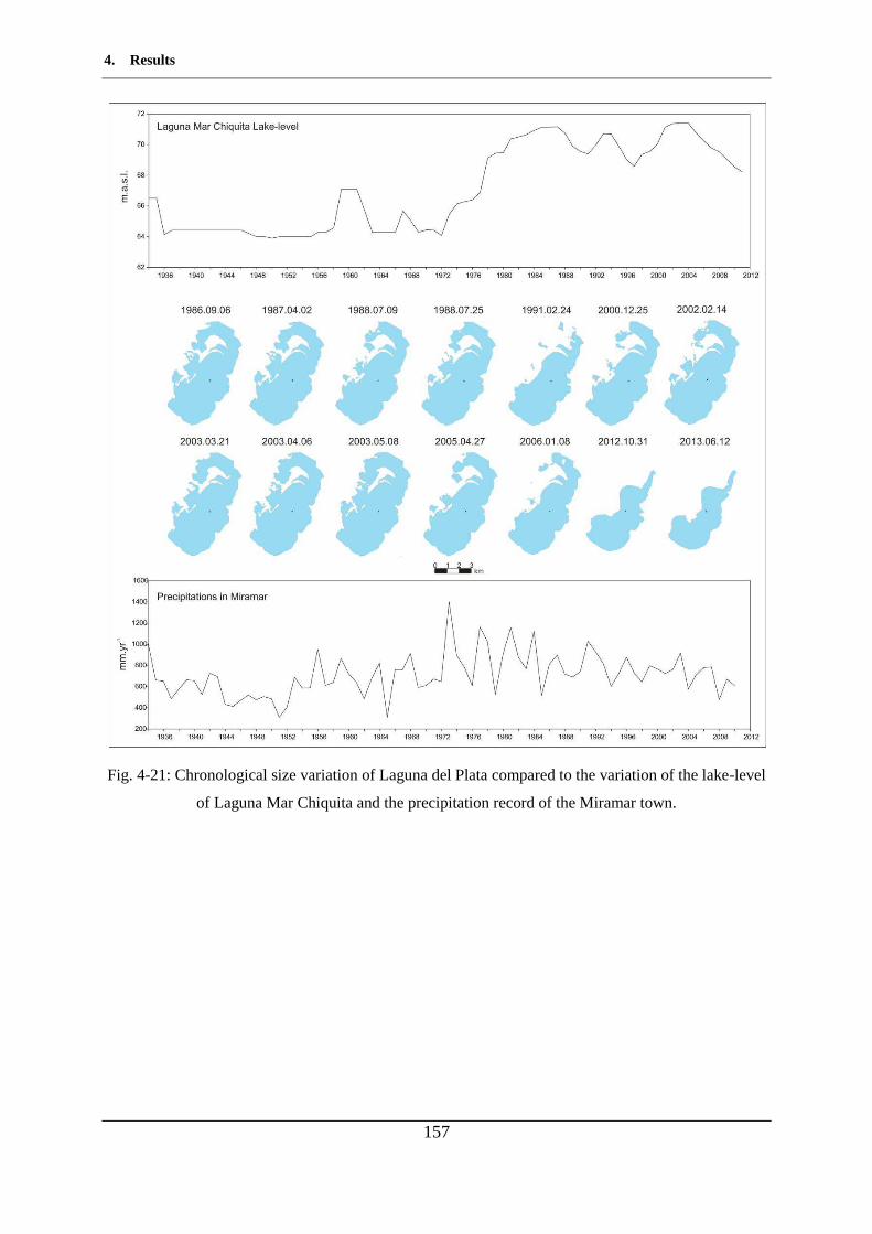
4. Results
157
Fig. 4-21: Chronological size variation of Laguna del Plata compared to the variation of the lake-level
of Laguna Mar Chiquita and the precipitation record of the Miramar town.
4. Results
158
4.5 Summary
Finally, the main results could be synthesized as follow:
Geochemical characterization of the Suquía River basin:
- The Suquía River waters show a physicochemical gradient from the headwaters to
downwaters until arriving to the Mar Chiquita system. Waters change from calcium-
sulphate to sodium-chlorided type.
- Saturation indexes for halite, anhydrite, gypsum, fluorite, dolomite, aragonite and
calcite become increasingly positive from headwaters to the lake.
- Soluble As concentrations have a good correlation with Li, Mg, Si, Ca, V, Br, Sr,
and Mo.
- As concentrations in river water show an increasing gradient from the upper basin
(crystalline rocks) to the lower basin (loessic sediments).
- Total particulate Hg concentrations measured in riverbed sediments collected from
tributaries and from the Suquía River higher at the basin’s catchments. Besides, HgTP
concentrations are ~7 times higher in the finer fraction (<63 µm) of the riverbed
sediments.
- Riverbed sediments are composed of quartz, albite, illite, microcline, perovskite and
pyrite, while in lake bottom sediments, evaporite salts such as halite and calcite are
identified along with quartz, albite, muscovite, and biotite.
Geochemical and sedimentological characterization of the sedimentary core
- Core dating allows to have a chronology for the last ~80 years.
- Mainly 3 zones in the core (corresponding to the years 1953 to 1969, 1969 to 2004
and 2004 to 2011 at the depth of 120 to 75, 75 to 16 and 16 to 0 cm respectively), are
identified based on marked variations of porosity, pH, Corg, Cinorg, sulphur as well as of
major and trace element concentrations.
- Minerals identified along the core are quartz, albite, calcite, muscovite, biotite and
halite as well as the clay minerals: montmorillonite and kaolinite. Pyrite is also present
as an accesory mineral.
4. Results
159
- Significant differences from 1970s until present are traduced in abrupt changes in the
grain-size distribution and elemental concentrations, particularly in total particulate
Hg and As as well as in their corresponding solid species.
- Hg associated with the oxidizable fraction (OM and sulphides) mostly explain the
HgTP concentration measured along the core, especially in the sediments accumulated
after 1970. Before this date, the acid-soluble Hg fraction is as important as the
oxidizable one. The concentration of Hg associated with the reducible fraction (Hg-
ascorbate) is neglible all along the core.
- There is an important Hg peak at 35 cm depth that cannot be explained by the
fractions analyzed through selective extractions, suggesting than another Hg-bearing
phase is present.
- As associated with the acid soluble fraction (As-HCl) is as important as the As
associated with the reducible fraction (As-ascorbate). However, none of them may
completely explain the concentrations of total particulate As along the core.
- There is an important As peak at 75 cm depth that coincides with a rise in Cinorg
and S concentrations.
- Increasing Hg accumulation rates are determined from 1970. Conversely, the As
accumulation rates show a decreasing trend in the same period.
- Laguna del Plata has reduced its size in over 50 % in the last 10 years.


5. Discussion
161
5. Discussion
5. Discussion
162
5. Discussion
163
The Laguna Mar Chiquita system has been widely studied as a whole but not many studies
have been performed in the small lake of Laguna del Plata. The sedimentary record of this
highly size-changing small lake helps to understand the hydrodynamics of its affluent (the
Suquía River), as well as the environmental and geochemical evolution of the basin with time.
Furthermore, the elemental proxies obtained in this hyper-saline lake serve as a comparative
means for lakes with similar characteristics.
5.1 The hydrogeochemistry of the Suquía River basin
The Suquía River plays an important role of carrying sediments and solutes from the
headwaters until it reaches the Laguna del Plata. Donwnflow, its chemical and
physicochemical composition changes due to the impact of the city of Córdoba, industries
located nearby and also due to the intensive agriculture activities. However, both lithology
and hydrology seem to be the most important factors controlling the geochemical evolution of
the river. Chemical alteration described in the river waters and sediments are linked with the
organic nature of the urban effluents that produce a marked consumption of dissolved oxygen
that originates anaerobic conditions inmediatly downflow the city of Córdoba (i.e., Pesce and
Wunderlin, 2000; Wunderlin et al., 2001; Monferrán et al., 2011; Merlo et al., 2011).
Besides the mentioned anthropogenic influence, a natural gradient represented by increasing
conductivity, TDS and pH values is observed downflow. Values of pH are close to neutral in
the headwaters while downflow it becomes more alkaline until reaching values of 9.5 in lake
waters. The mentioned trend is more likely attributed to the lithology that also controls the
major chemical composition of waters in the basin. At the basin’s catchment, where igneous
and metamorphic rocks prevail, waters are of the calcium-bicarbonate-type and change to the
sulphate type in the middle stretch of the river after crossing the city of Córdoba where
lithology is dominated by loessic deposits. Near to the lake area, waters show their maximum
concentrations in TDS and the highest conductivities in the basin changing from fresh water
to saline water (30-50 g L-1) in the Laguna Mar Chiquita and into brines ( 50 g L-1). The
interaction with lithology also controls the saturation of the water in the basin with respect to
different minerals. Piovano et al., (2009) indicate that drier conditions predominate in the
region from 2003. The Mar Chiquita systems reduced its size considerably and these changes
can be seen in figures Fig. 4-19 and Fig. 4-20. Laguna del Plata has reduced its size at least
50 % in the last 10 years. These changes are in agreement with the precipitation record (Fig.

5. Discussion
164
4-21) measured in Miramar town that shows a humid trend early 1970s and a reduction in
precipitations early 2000s. The changes in water input carried a consequent increase in
salinity and precipitation of salts. This climatic trend gives high probability to reach
supersaturation conditions to allow precipitation of minerals like dolomite, aragonite and
calcite (Table 4-2) as it found in river water samples and that increase in these minerals while
closer to the lake. Dissolution of salts such as halite could occur in the basin and even if
saturation for this mineral is not reached, values tend to be less negative downflow.
The physicochemical gradient that was observed in lake waters with depth can be explained
by the existence of a microbial mat that covers the bottom of the lake. This mat corresponds
to the contact zone between the water and the bottom of the lake (Bucher and Abril, 2006). In
salt lakes, this zone favours the development of a rich community of bacteria, algae and
microscopic animals (Jonkers et al., 2003) and it is where an important amount of primary
productivity occurs (Hammer, 1986). Even if the water column in both lakes is well
oxygenated as cause of the dominant winds, the diminution of dissolved oxygen (
Table 4-1) between water in the surface and in the bottom of the lake proves its existence.
Soluble trace metals were also determined in waters of the basin. Focus was made on As and
some other elements usually associated with it in groundwaters in contact with loessic
sediments accumulated in the Chaco Pampean Plain (see section 2.2.4). In waters of the
Suquía River basin, As concentrations are below the WHO drinking water guideline (10 µg L-
1) in most of the sampling points located in the catchments. Nevertheless, As concentrations
reach values that exceed over 2 times the drinking water guideline (22.4 µg L-1) in the lower
part of the basin (RS9). Especially in the middle and lower part of the basin, higher As
concentrations are assigned to a longer water-rock interaction but also to the presence of
loessic sediments. As concentrations measured in surface waters are markedly lower than
those measured in groundwaters (i.e. Nicolli et al., 2012 and references therein) due to the
shorter time of contact between water and sediments. The source of As in surface waters is
likely associated with the loessic sediments, as suggested by the high correlation values that
exist between As and some other trace elements such as Li, V and Mo (Table 4-5). The good
correlation between As and this elements has also been reported in groundwaters of the Chaco
Pampean Plain, and this behaviour was atributted to the dissolution of volcanic glass grains
spread in the loess matrix (Nicolli et al., 2010, 2012).
5. Discussion
165
5.2 The geochemistry of riverbed sediments in the Suquía basin
Sediments play an important role as sinks of trace metals and therefore they constitute
excellent archives of past contamination (Castelle et al., 2007). Besides, they may act as
secondary sources, releasing them again into solution under suitable environmental conditions
(Schäfer et al., 2010). The concentration of trace metals in sediments is also linked to the
particle size; generally it increases with decreasing particle size (Brook and Moore, 1988).
Mineralogical composition of riverbed sediments (Fig. 4-4) reveals the presence of quartz,
albite, illite, microcline, and accessory minerals such as perovskite and pyrite. All these
minerals are former components of the crystalline rocks of the Sierras Pampeanas Range
located in the western margin of the study area, thus reflecting the weathered materials that
are transported downstream. Minerals identified in the lake bottom sediments are mostly the
same but some secondary minerals such as calcite and halite are also identified. These
minerals formed by precipitation from the supersaturated lake waters (Table 4-2)
Both, silty and sandy fractions show that the higher Hg concentrations are located in the upper
part of the basin where values are over 61 µg kg-1 while in the middle stretch of the Suquía
River and lower part of the basin, Hg concentrations remain low ( 61 µg kg-1). Even if higher
Hg concentrations are located in the upper part of the basin, values are among those
considered within the limits of natural total particulate Hg in sediments (150 µg kg-1, Schäfer
et al., 2006). The upper part of the basin is located in the Sierras Pampeanas Range where
exists the presence of sulphur mineralization (Mutti et al., 2005) and could be the source of
this Hg. Besides, part of the sediment carried by the river and that contains Hg, could be
deposited in the San Roque Dam and stop the transport downflow. Furthermore, the industries
and city input in the middle stretch and lower part of the Suquía River seems to be negligible
due to that Hg concentrations are more or less constant before and after crossing the city of
Córdoba until the river mouth in Laguna de Plata.
The geochemistry of sediments is marked by the imprint of the dominant rocks in the area. Hg
concentrations are below the limit of natural values. Nevertheless, higher concentrations occur
in the mountainous area associated to sulphur mineralization but punctual anthropogenic
source was not detected.
5. Discussion
166
5.3 Chronology and sediment deposition of the sedimentary core
The sedimentary core taken in Laguna del Plata (LP) where the Suquía River mouths allows
to understand more about the sedimentation processes that took place in this lake.
The Mar Chiquita system has suffered dramatic hydrological changes. Piovano et al. (2009)
calculated that Laguna Mar Chiquita (LMC) had ~1000 km2 prior to the 1970s and that it
increased its size up to ~6000 km2 in the wettest periods (like in 2003). Nowadays, Laguna
Mar Chiquita covers an extension of ~2000 km2. Concerning Laguna del Plata,
reconstructions of the size of the lake have not been previously calculated. However, the
climatic changes that affected the region have transformed the physiognomy of this lake
reducing its size in more than 50 % (from 29.9 to 13.8 km2) in the last 10 years (section
4.4.2). These changes are also registered in the sediments, thus the chronology was
determined along the sedimentary core for better identify the events. The core dating
estimates a sedimentary succession of ~80 years. Furthermore, it evidences an average
sedimentation rate of 1 cm y-1 but in general two different sedimentation rates are noticed.
One with values around 1.2-1.5 cm y-1 that occur before the year 1975 (up to 65 cm depth)
and the other one with values up to 3 cm y-1 determined in the upper part of the core. The
latter is in agreement with the negative hydrological conditions that prevailed in the region
since 2003. Before 1975 Laguna Mar Chiquita and Laguna del Plata did not have a
hydrological connexion. However, Laguna del Plata continued receiving the sedimentary
input from the Suquía River. Regarding the water balance, main contributions to the lake were
from the Suquía River and groundwater discharges (Troin et al., 2010). In contrast and due to
its larger extension, Laguna Mar Chiquita sedimentation rates are much lower and vary
between 0.25-0.34 cm y-1 during lowstands and between 0.77-1.12 cm y-1 during highstands
(Piovano et al., 2002; 2006). These differences in sedimentations could be due to the position
of the sedimentary core taken at LP11-1 sampling station. This location faces the entrance of
the river to the lake and the contribution of sediment could be important.
In the early 1970s the climatic conditions started to change, and the dry period was replaced
by a humid period (Troin et al., 2010) that lead to an augmentation in the Mar Chiquita lake-
level. Near the year 1975 alternating re-connections and disconnections between both lakes
alternated may have occurred which are evidenced in the sedimentary record by the alternance
of light and dark laminations at the depth of 70 cm (Fig. 4-6). Since 1976 there was a total
reconnection between LP and LMC that persist until nowadays. However, since 2003 the
5. Discussion
167
water budget started to decrease (Piovano et al,.2004, 2009) leaving a small channel that
connects both lakes and that gets increasingly narrow (Fig. 4-20).
When comparing the grain-size distribution in sediments accumulated in Laguna del Plata
with the historical LMC lake-level variation (Fig. 4-8c) it is possible to deduce that
predominating fine silt correspond to periods where the lake-level was stable for a short
period of time. Medium to coarse silt fractions are related to periods were the lake-level
started to rise, either if it was after a long or a short dry period. This clearly represents an
enhanced transport of larger particles from the basin due to the higher water energy and
higher runoff. Different water input budgets are traduced as well in the porosity values (Fig.
4-8e). The lower part of the core is represented by almost constant porosity values but from
the beginning of the wet period they increase. Higher water budget generated an increase in
primary production that it is traduced in higher Corg inputs that may additionally control the
porosity values. Corg values registered in the lower part of the core are almost constant
(0.83 % ± 0.22) and in addition they are concomitant to the scarce precipitations and the
high water salinity. These values are markedly lower than those previously reported for some
Patagonian lakes. In Northern Patagonia, Corg oscillated between 6 and 8 % (i.e. Ribeiro
Guevara et al., 2010) while in the South, values varied between 12 and 15 % (Hermanns and
Biester, 2013). Corg values are important indicators of Hg input from soil erosion in the upper
watershed of lakes due to the high affinity of this element for organic matter (Driscoll et al.,
1995; Rydberg et al., 2010; Teisserenc et al., 2010).
The bottom part of the core represents the period that spans the years between 1935 and 1975.
According to Cioccale (1999) present climate conditions in Argentina started around the
middle 19th Century after the end of the Little Ice Age which was characterized by cold and
arid episodes alternated with short humid events. In this arid period great amount of loess
(from 45 to 145 g m-2 y-1) were transported from the Andes to the Chaco Pampean Plain
(Zárate, 2003; Maher et al., 2010) and could have influenced the input of larger particles into
the lake. Furthermore, Martínez et al. (1994) and Kröhling and Iriondo (1999) identified that
the west part of the Mar Chiquita system is composed by aeolian sands (Fig. 1-8).
Recent studies performed by Gaiero et al. (2013) show that sediments with origin in the Puna-
Altiplano region (north of Argentina) can be transported for long distances thanks to the
dominant air masses movements in South America. Two dusts events were monitored in 2009
and 2010 and even if their plumes were reduced ~50 % along its trajectories, their signals
were registered 24 h after the beginning of the event in places located ~1300 km SE from the
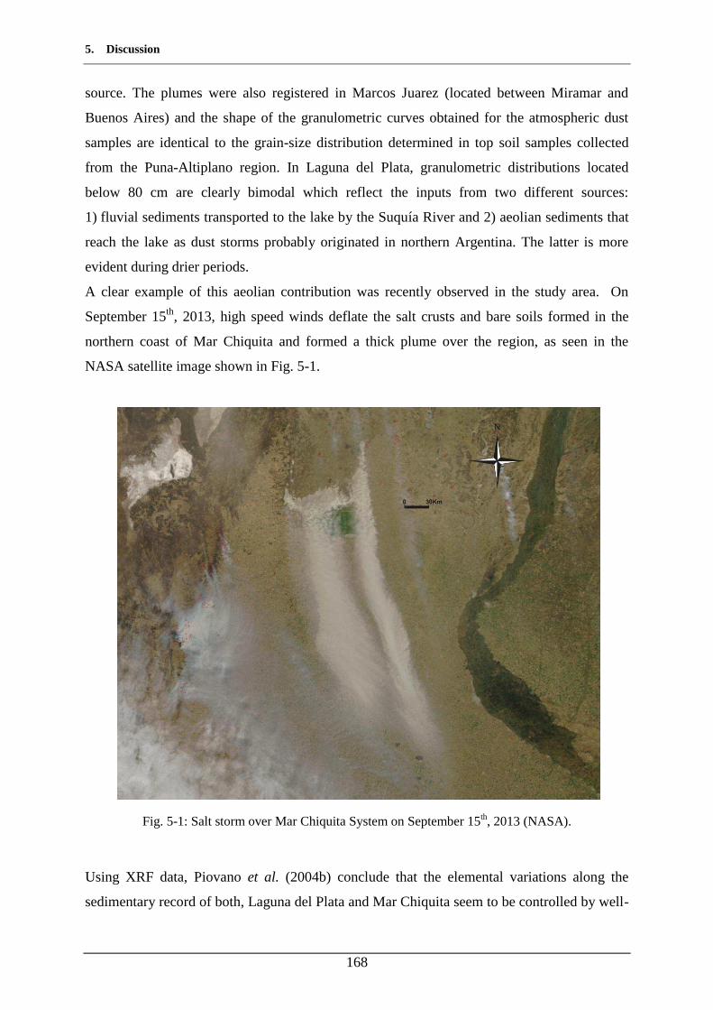
5. Discussion
168
source. The plumes were also registered in Marcos Juarez (located between Miramar and
Buenos Aires) and the shape of the granulometric curves obtained for the atmospheric dust
samples are identical to the grain-size distribution determined in top soil samples collected
from the Puna-Altiplano region. In Laguna del Plata, granulometric distributions located
below 80 cm are clearly bimodal which reflect the inputs from two different sources:
1) fluvial sediments transported to the lake by the Suquía River and 2) aeolian sediments that
reach the lake as dust storms probably originated in northern Argentina. The latter is more
evident during drier periods.
A clear example of this aeolian contribution was recently observed in the study area. On
September 15th, 2013, high speed winds deflate the salt crusts and bare soils formed in the
northern coast of Mar Chiquita and formed a thick plume over the region, as seen in the
NASA satellite image shown in Fig. 5-1.
Fig. 5-1: Salt storm over Mar Chiquita System on September 15th, 2013 (NASA).
Using XRF data, Piovano et al. (2004b) conclude that the elemental variations along the
sedimentary record of both, Laguna del Plata and Mar Chiquita seem to be controlled by well-
5. Discussion
169
known hydrological fluctuations that affected the region during the 20th Century. Sediments
accumulated in the bottom part of the LP core up to 74 cm represent the sedimentation before
1970s when LP was completely isolated from LMC and the inputs were mainly from the
Suquía River. In agreement with these data, XRF signals measured in the core retrieved for
this study (Fig. 4-11) reflect this single contribution to the sedimentary record. The
augmentation of the regional precipitations that allowed the LMC lake-level to rise driving the
re-connection of both lakes around 1976, generated a change in the sedimentation pattern
overall the Laguna Mar Chiquita system (Piovano et al., 2002; 2004a). Rising lake-level
likely triggered the strong variations in Al, Si, K, Ti, Fe, and Zr concentrations measured in
the LP core between 74 to 16 cm depth, reflecting a higher contribution from detrital input
due to soil or fluvial-bank erosion in the basin’s catchments. Several authors (Rothwell and
Rack, 2006; Böning et al., 2007; Moreno et al., 2007; Löwemark et al., 2011) coincide that
variations of terrigenous elements such as Al, Si, K, Fe, and Ti are likely the consequence of
inputs of allocthonous materials. The evaporitic signal can be inferred from Cl and Ca signals,
which show constant profiles in the lower part of the core. An increment in the water budget
could have contributed to the dissolution of salt crusts that are usually formed on top of the
muddy sediments in drier periods next to the lake rising the signal of these elements, such is
the case around 70 cm depth. The profiles of both elements in the upper part on the core (last
16 cm) show an augmentation of the signal toward the top. At the same time, these last 16 cm
correspond to the period that spans from 2003-2004 to date. LMC lake-levels started to
continuously decrease from 71.80 to 67.45 m.a.s.l. (Troin et al., 2010) and rising the salinity
from 27.0 g L-1 (Bucher and Bucher, 2006b) to 67.3 g L-1 (Biglia et al., 2013) that could
suggest a concentration of these elements in the sediments in LP.
Finally, the analysis of the sedimentary core showed to have a relation between sedimentation
rates, grain-size distribution and chemical variations with changes of hydrological conditions
through ~80 years:
- Until early 1970s dry and arid conditions prevailed and LP and LMC were
hydrologically disconnected,
- From ~1976 to 2003-2004 wet conditions predominated and a lake-level followed
with the consequent reconnection of both lakes,
- From 2003 until now, a new dry period started with the decrease in both lake-levels.
LP and LMC are still connected through a narrow channel.
5. Discussion
170
5.4 The historical record of Hg and As in sediments accumulated in
Laguna del Plata during the last ~80 years
In connection with the hydrological variations previously identified and lithological context
of the study area, changes in concentrations of Hg and As in the core are analyzed, as well as
their souces and carrying phases.
5.4.1 Mercury
Using the sedimentological features, mineralogical composition, dating and selective
extraction procedures, it was possible to reconstruct the historical record of Hg in the Suquía
River basin and analyze the results on the context of the hydrological change.
Sediments accumulated in the lake before the 1970s show rather constant and very low HgTP
concentrations (Fig. 4-12). During this period of high aridity and low lake levels, particles
transported by the Suquía River exclusively settled in the Laguna del Plata due to the absence
of hydraulic links between the latter and Laguna Mar Chiquita. The values of Hg registered in
the lower part of the core are low compared with those measured in the upper part. However,
they are similar to the concentrations measured in the riverbed sediment samples collected
along the Suquía River watershed and also in a sample of atmospheric dry deposition
collected in a pluviometric captor located near the lake.
According with selective extraction results, the main Hg carrying phases in sediments
accumulated before 1970, are probably secondary sulphides, especially in the 105-85 cm
depth range (Fig. 4-12). This is consistent with X-Ray Difractometry data that shows the
presence of pyrite in the base of the core (Fig. 4-10), indicating that the precipitation of
authigenic sulphides occurred under dominant anoxic conditions, likely produced by bacterial
activity at the water-sediment interface. Similar conditions were found in different lakes
around the world, for example Green Lake in United States (Suits and Wilkin, 1998), Baptiste
Lake, Canada (Manning et al., 1999), Qinghai Lake, China (Sugimori et al., 2007) or Lake
Kinneret, Israel (Nowaczyk, 2011).
Bucher and Bucher (2006b) studied the bottom lake muddy sediments from Laguna Mar
Chiquita and they attributed the typical black colour of the sediments to the presence of
bacteria that live in the microbial mat of the bottom of the lake. These bacteria include not
only the bacteria (Cyanobacteria) sensu strict but the other two fundamental domains:
5. Discussion
171
Archaea (single-celled microorganisms) and Eukaryote (cells containing a nucleus) (Bucher
and Abril, 2006).
Hg can be bound to sulphides -mostly pyrite-, by adsorption (e.g., Bostick and Fendorf, 2003;
Doyle et al., 2004; Borah and Senapati, 2006; Ozverdi and Erdem, 2006) in a wide pH range
(Behra et al., 2001) forming Hg-Cl and Hg-OH complexes (Behra et al., 2001; Bower et al.,
2008) and this process is favoured by the high water salinity and alkalinity (Bower et al.,
2008). Elevated salinity (380 g L-1; Piovano et al., 2004a) and alkaline chloride–sulphate
sodium type waters (Martínez 1991) represent the geochemical conditions predominating
during lake lowstands. Mercury associated with the residual fraction not extracted by the
single extraction approach, attributed to the non-reactive crystalline matrix, was very low
(close to zero) in the sediments accumulated before the 1970s, indicating that nearly all Hg
deposited during that period was potentially bioavailable.
In sediments accumulated after the 1970s, the HgTP concentrations (Fig. 4-12) are clearly
higher than downcore (almost ~4 times in average). This coincides with the beginning of an
increasingly humid period in the region, and a concomitant rise in the lake system levels.
During this period increased erosion and riverborne particle transport in the Suquía River
watershed also occurred. The values in this section of the core are within the range measured
in lakes of the Argentinean Patagonia and in other remote regions of the world that are not
directly affected by human activity (e.g. Ribeiro Guevara et al., 2010; Yang et al., 2010;
Conaway et al., 2012; Hermanns and Biester, 2013).
In the 74-40 cm depth range, Hg is predominantly associated with sedimentary organic
matter. Within this depth range, the Corg values are highly variable, but higher in average than
the values measured in the bottom of the core. This trend reflects increasing Hg
concentrations related to increased lake primary productivity but also to increased soil erosion
and transport rates of riverborne particles in the Suquía River (Piovano et al., 2009). The
latter is also manifested through the presence of a major proportion of Hg associated with Mn
and Fe oxy-hydroxides. Amorphous or poorly crystalline oxides are known as sinks for metal
contaminants owing to their large surface area and/or microporous structure (Axe and Trivedi,
2002). For example, ferruginous nodules, formed during the lateritic weathering process, used
to contain elevated Hg contents (Roulet and Lucotte, 1995; Roulet et al., 1998; De Oliveira et
al., 2001; Brabo et al., 2003). The adsorption of Hg onto Fe oxides has been widely reported,
and it is preferentially produced under alkaline conditions (e.g., Schuster, 1991; Tiffreau et
al., 1995).

5. Discussion
172
Hydrochemical conditions in the lake during highstands corresponded to alkaline chloride–
sulphate sodium type waters, supersaturated in calcite and occasionally in gypsum (Martínez
et al., 1994) as it was found in Laguna Mar Chiquita (Piovano et al., 2004b). Martínez (1991)
and Piovano et al. (2002) conclude that calcite disseminated in sediments accumulated in the
Laguna del Mar Chiquita is authigenic and formed by precipitation from calcite
supersaturated lake waters, conditions that predominate even during the most dilute stages of
the lake. In the case of Laguna del Plata, gypsum was not found in the sediment. This is
probably due to the diluting effect that Suquía River exerts on LP waters that prevents
arriving to the necessary concentrations to form gypsum. Durigneux (1978) indicated the
presence of sodium sulphates in LMC but the specific salts were not specified. However, due
to the recent retraction of the lake water, muddy sediments from the bottom of the lake are
exposed. The analysis of these sediments showed the presence of sodium sulphate minerals
that appear as efflorescences Biglia et al. (2013). These minerals are Thenardite (NaSO4) and
Mirabilite (NaSO4·10H2O), that, although frequent in saline lakes were unknown in LP until
now.
Mercury profile show maximum HgTP at ~38 cm, i.e. in the depth range roughly attributed to
records of the years 1990-1995. The residual Hg fraction shows maximum levels (>50% of
HgTP) at ~35 cm depth, suggesting an episode with major transport and deposition of non-
reactive Hg-bearing phases during the 1990s just after the episode responsible of the HgTP
maximum. Accordingly, the maximum HgTP levels together with minimum HgH202/HgTP and
relatively low HgHCl/HgTP suggest dominance of Hg-bearing phases not accessible to the used
selective extractions. Among the different Hg sources described in natural systems, volcanic
emissions are a major issue (i.e., Fitzgerald and Lamborg, 2003, Selin, 2009). Due to the
proximity to the Andean volcanic system and its well known influence on the study area (e.g.
Gaiero et al., 2007; Osores et al., 2011) volcanic eruptions could account for this observation.
In fact, the eruption record of the past 100 years indicates that the observed peak could reflect
Hg inputs from the eruption of the Chilean Hudson and Láscar volcanoes located in Chile.
The first one is situated at 45°54’S - 72°58’W and erupted in two phases in August 1991,
producing 4.3 km3 of pyroclastic material during one of the major eruptions of the 20th
Century (Wilson et al., 2011). The second one is located at 23°22’S – 67°44’W and started its
activity in 1984 culminating with a major explosive eruption in April 1993. This last eruption
generated a column between 5 and 25 km above the volcano (Matthews et al., 1997). In both
cases, the respective ash plumes were documented to have reached the Laguna del Plata
region thus the Hg associated to volcano-clastic particles could have settled as wet or dry
5. Discussion
173
deposition in the Suquía River watershed. This could explain the peak of HgTP observed in the
core (between 37.2 and 30.2 cm) and its preferential association with non-reactive particles in
the sediments accumulated in the years following the eruption.
5.4.2 Arsenic
In what concerns to As, it shows an opposite behaviour with respect to Hg. The higher
concentrations are located in the lower part of the core that corresponds to dry climate periods
and higher pH values. As it was previously mentioned, the sediments of the lower part of the
core have two provenances fluvial and aeolian. In this dry period most of the As contributions
could be attributed to the input of the Chaco Pampean Plain loess that was transported to
Laguna del Plata by winds from nearby regions. The average As-tot concentration measured
in the core is 20.953 ± 18.006 mg kg-1, which is consistent with the As concentrations
reported in loessic sediments of the Chacopampean Plain (Nicolli et al., 2012 and references
therein), This value results more than 4 times higher than the As concentrations reported in
some other lakes of the world (i.e., Cook et al., 1995; Smedley and Kinniburgh, 2002 and
references therein)
It is possible as well that a small part of the As deposited in the salt crusts around the lake was
blown away and re deposited on the lake or re entered in solution. In the other hand, lower As
concentrations occur in the middle and upper part of the core when the hydrological
conditions started to change. Part of the As retained in the salt crusts formed around the lake
could be wash-out during the first precipitation events and also at increasing lake-levels.
The results of the As-asc and As-HCl extractions (Fig. 4-14) explain up to ~46 and ~78 %
respectively of the As-tot. This suggests that As seems to be adsorbed onto reactive Fe and
Mn hydr(oxides) all along the sedimentary core. Nevertheless, the relationships found
between As, Fe and Mn extracted from the ascorbate fraction (Fig. 4-16), show that As
correlates better in the lower part of the core. Moreover, there is a difference between As-asc
and HCl fractions in the lower part of the core where As-asc explains in average 5.83 ±
16.42 % and As-HCl 59.04 ± 12.93 % of the As-tot. It is possible to think that due to the
presence of pyrite and the high sulphur concentrations (Fig. 4-8) at this depth, part of the As
is associated to sulphides. Several authors have reported the association between As and
5. Discussion
174
pyrite (Bostick and Fendorf, 2003; Doyle et al., 2004; Rickard and Morse, 2005; Özverdi and
Erdem, 2006; Charlet et al., 2011), wich is enhanced under anoxic conditions that usually
prevail in the mat located at the bottom lakes (Couture et al., 2013). The presence of sulphur
reducing bacteria also play an important role in controlling the soluble trace metal
concentrations, as they promote the precipitation of secondary sulphides Rittle et al, (1995),
Oremland et al., (2000), Kirk et al., (2004).
With the increase of water budget in the humid period, fluctuations in Corg and Cinorg contents
are noticed (Fig. 4-8f-g) around 74 cm. Moreover, a decrease of the Fe and Mn acid soluble
and reducible fractions (Fig. 4-13) is registered. It has been demonstrated (e.g: Cheng et al.,
1999; Fernández-Martínez et al., 2006; Román-Ross et al., 2006) that As may co-precipitate
along with calcite and gypsum. Furthermore, some authors (Moon et al., 2004; Di Benedetto
et al., 2006) showed that when Ca/As molar ratio is 1 favours the association of As with
calcite or kaolinite minerals. When regarding the chemistry and mineralogy of the water and
sediments of the lake, gypsum is not found and, at least in Laguna del Plata, water is
subsaturated in this mineral (Table 4-2). Nevertheless, water is always superaturated (Table
4-2) in calcite and this mineral is frequent in the sediments (Fig. 4-10). Clay minerals such as
illite or kaolinite were also found in sediments of the basin and in the lake. Some authors
indicate that calcite-coated clays, such as illite, may adsorb arsenate ions under alkaline
conditions (Bugueño et al., 2014).
The As acid-soluble fraction show a peak that is coincident with another peak of Cinorg (
Fig. 4-15a), strongly suggesting that part of the As may be immobilized by co-precipitation
with calcite.
Although the As-HCl fraction can explain over 75 % of the total As (Fig. 4-14) there is part of
residual As (i.e., crystalline lattice) that could not be explained neither to As-HCl nor As-asc.
Rickard and Morse (2005) showed that pyrite partially dissolves when treated with HCl.
Thus, it could exist part of As adsorbed onto the un-dissolved pyrite fraction that is not
released in the extraction.

6. Conclusion
175
6. Conclusion

6. Conclusion
177
This work has led to the study of behavior and the origin of mercury and arsenic, two trace
elements present in the Mar Chiquita system. Based on the results previously discussed, an
hydro-geochemical model concerning the functioning of Mar Chiquita system can be
proposed (
Fig. 6-1). This is a modification of the original model proposed by Piovano et al. (2004a,b)
and was adjusted in Stupar et al. (2013) that aims to include the main Hg and As bearing
phases identified previously in the area and.
Precipitation (P) and evaporation (E) are represented with arrows, whose relative lengths are
proportional to their volume. The higher river runoff, which occurred after the 1970s, is
indicated by a solid arrow, whereas dotted arrow indicate comparatively low inputs that
prevailed in the dry period. The thickness of the arrows associated with different Hg and As-
bearing phases recognized in the studied area is proportional to their respective importance.
During the dry conditions and low lake-levels that predominated in the study area before the
1970s, inputs of Hg to the lake corresponded mainly to contributions from natural sources
such as Hg-bearing particles (particularly sulphides) that were transported to the lake from the
Suquía River upper basin and atmospheric Hg (dry deposition). Under high stand conditions
(after 1970s), these two sources increased their contributions due to increasing precipitation
(wet deposition) and higher soil erosion in the catchments, but also to increasing global Hg
flux. The more humid conditions lead to increased lake primary productivity and hence, a
higher affinity of Hg for organic matter particle is found in sediments accumulated during this
period.
Arsenic instead is mainly associated to Mn and Fe (hydr)oxides in the aquatic phase favoured
by the high pH conditions of the lake during low and high stands. Furthermore, under more
arid conditions, the As input to the lake was enhanced by the prevailing winds that carried As-
rich loess particles. Under more humid conditions the As input from the atmosphere is less
important and it is mostly introduced into the lake associated with riverborne particles.
Besides being bounded to Mn and Fe, As is associated to pyrite in the lower part of the core
and to calcite in the middle and upper parts. The residual As that could not be explained by
the selective extractions may be attached onto non reactive pyrite.
The sources of Hg and As in the Laguna del Plata sediments are mostly assigned to natural
sources. In the case of Hg a contribution from global inputs should be considered, as well as
from some other local anthropogenic sources, that became increasingly important after the
1970s when an incipient industrial development started in the region. The volcanic activity
occurred early 1990s could have increased the signal of Hg. Regarding As, the main input is
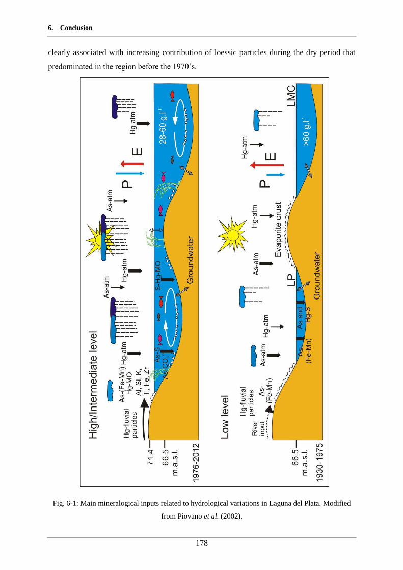
6. Conclusion
178
clearly associated with increasing contribution of loessic particles during the dry period that
predominated in the region before the 1970’s.
Fig. 6-1: Main mineralogical inputs related to hydrological variations in Laguna del Plata. Modified
from Piovano et al. (2002).
6. Conclusion
179
This study allowed to have a global understanding of the sources and dynamic of Hg and As
in Laguna del Plata. As well as the important role that climate and hydrological balance exert
controlling the behaviour of these two elements. This study also enabled to identify the main
Hg and As bearing phases through the utilization of selective extractions, finding that
sulphurs and pyrite in special, is a key mineral that acts as a trap. With these results, this work
clearly contributes to better interpret the functioning of this small salt lake.
The work carried out in this thesis has allowed to submit two articles in indexed journals that
are added as annexes:
Annexe A: 1st article: Stupar, Y.V., Schäfer, J., García, M.G., Schmidt, S., Piovano, E.,
Blanc, G., Huneau, F., and Le Coutumer, P. Historical mercury trends
recorded in sediments from the Laguna del Plata, Córdoba, Argentina.
Journal: Chemie der Erde / Geochemistry. Status: accepted for
publication, http://dx.doi.org/10.1016/j.chemer.2013.11.002.
Annexe B: 2nd article: Stupar, Y.V., García, M.G., Schäfer, J., Schmidt, S., Piovano, E.,
Blanc, G., Huneau, F., and Le Coutumer, P. Identificación de fases
portadoras y flujos de mercurio en el registro sedimentario de la
Laguna del Plata, región central de Argentina. Journal: Revista
Mexicana de Ciencias Geológicas. Status: accepted for publication.
6. Conclusion
180
6.1 Perspectives
In terms of the perspectives of this work, the modalities of operation of this hydro-
geochemical model could be improved by answering the following questions:
- What is the role of organic matter in the speciation of As and Hg?
- What is the contribution of As from atmospheric dust and the loessic formations?
- What are the mechanisms that determine the speciation of As in highly saline
environments?
- What is the role of pH and ionic strength in the aqueous and solid phases of these two
elements?
However, this work constitutes a first approach in the study of the origin of these trace metals
in the Laguna del Plata and the associated Suquía River system. The question regarding their
evolution is still a matter of study. Nevertheless, understand the (bio)geochemical processes
involved in the reactivity, fate and toxicity of Hg and As could lead to answer it.

Bibliography
181
Bibliography
Bibliography
182
Bibliography
183
A
Aceituno, P., 1988. On the functioning of the Southern Oscillation in the South American sector. Part
I: surface climate. Monthly Weather Review. 116, 505–524.
Aceñolaza, F.G. and Toselli, A., 1976. Consideraciones estratigráficas y tectónicas sobre el Paleozoico
inferior del Noroeste Argentino. 2° Congreso Latinoamericano de Geología, Actas 2: 755-763,
Caracas.
Ahmed, R., May, K. and Stoeppler, M., 1987. Ultratrace analysis of mercury and methylmercury
(MM) in rainwater using cold vapour atomic absorption spectroscopy. Fresenius Z. Analytical
Chemistry. 326, 510-516.
Alborés, A.F., Cid, B.P., Gómez, E.F. and López, E.F., 2000. Comparison between sequential
extraction procedures and single extractions for metal partitioning in sewage sludge samples.
Analyst. 125, 1353-1357.
Amin, O., Ferrer, L. and Marcovecchio, J., 1996. Heavy metal concentrations in litteral sediments
from the Beagle Channel, Tierra del Fuego, Argentina. Environmental Monitoring and
Assessment 41 (3), 219-231.
Arnórsson, S., 2003. Arsenic in surface- and up to 90°C ground waters in a basalt area, N-Iceland:
Processes controlling its mobility. Applied Geochemistry. 18 (9), 1297-1312.
Appelo, C.A.J. and Postma, D., 2005. Geochemistry, Groundwater and Pollution, Second Edition.
Taylor & Francis. The Netherlands. pp.649.
Appleby, P.G., 2001. Chronostratigraphic techniques in recent sediments. W. M. Last & J. P. Smol
(eds.).Tracking Environmental Change Using Lake Sediments. Volume 1: Basin Analysis,
Coring, and Chronological Techniques. Kluwer Academic Publishers, Dordrecht, The
Netherlands.
Arribére, M.A., Ribeiro Guevara, S., Sánchez, R.S., Gil, M.I., Román Ross, G., Daurade, L.E., Fajon,
V., Horvat, M., Alcalde, R. and Kestelman, A.J., 2003. Heavy metals in the vicinity of a chlor-
alkali factory in the upper Negro River ecosystem, Northern Patagonia, Argentina. Science of
the Total Environment. 301 (1-3), 187-203.
Audry, S., Blanc, G. and Schäfer, J., 2005. The impact of sulphide oxidation on dissolved metal (Cd,
Zn, Cu, Cr, Co, Ni, U) inputs into the Lot-Garonne fluvial system (France). Applied
Geochemistry 20 (5), 919-931.
Audry, S., Blanc, G., Schäfer, J., 2006. Solid state partitioning of trace metals in suspended particulate
matter from a river system affected by smelting waste drainage. Science of the Total
Environment. 363, 216–236.
Azcue, J.M., Murdoch, A., Rosa, F. and Hall, G.E.M., 1994. Effects of abandoned gold mine tailings
on the arsenic concentrations in water and sediments of Jack of Clubs Lake, BC. Environmental
Technology. 15, 669–678.
Bibliography
184
Axe, L. and Trivedi, P., 2002. Intraparticle Surface Diffusion of Metal Contaminants and their
Attenuation in Microporous Amorphous Al, Fe, and Mn Oxides. Journal of Colloid and
Interface Science. 247 (2), 259-265.
B
Bagli, S. and Soille, P., 2004. Automatic delineation of shoreline and lake boundaries from Landsat
satellite images. Proceedings of initial ECO-IMAGINE GI and GIS for Integrated Coastal
Management, Seville 13th–15th May 2004.
Behra, P., Bonnissel-Gissinger, P., Alnot, M., Revel, R. and Ehrhardt, J.J., 2001. XPS and XAS study
of the sorption of Hg(II) onto pyrite. Langmuir 17, 3970-3979.
Benson, L.V. and Spencer, R.J., 1983. A Hydrochemical Reconnaissance Study of the Walker River
Basin, California and Nevada. USGS Open File Repport, 83–740. United States Geological
Survey, Denver.
Berbery, E.H. and Collini, A., 2000. Springtime precipitation and water vapour flux over southeastern
South America. Monthly Weather Review. 128, 1328-1346.
Berbery, E.H. and Barros, V., 2002. The hydrologic cycle of the La Plata basin in South America.
Journal of Hydrometeorology. 3, 630-645.
Bermond, A.P., 1992. Thermodynamics applied to the study of the limits of sequential extraction
procedures used for the speciation of trace elements in sediments and soils. Environmental
Technology. 13 (12), 1175-1179.
Bertoldi de Pomar, H., 1953. El origen de la Laguna Mar Chiquita. Doctoral Tesis. Unpublished.
Universidad Nacional de Córdoba.
Bhattacharya, P., Claesson, M., Bundschuh, J., Sracek, O., Fagerberg, J., Jacks, G., Martin, R.A.,
Storniolo, A.R. and Thir, J.M., 2006. Distribution and mobility of arsenic in the Río Dulce
alluvial aquifers in Santiago del Estero Province, Argentina. Science of the Total Environment.
358, 97-120.
Biester, H., Kilian, R., Franzen, C., Woda, C., Mangini, A. and Schöler, H.F., 2002. Elevated mercury
accumulation in a peat bog of the Magellanic Moorlands, Chile (53°S) - an anthropogenic signal
from the Southern Hemisphere. Earth and Planetary Science Letters. 201 - 609-620.
Biglia, H.O., Colombo, F., Piovano, E. and Córdoba, F., 2013. Thénardita y Mirabilita en precipitados
químicos litorales de la Laguna Mar Chiquita, Córdoba (Argentina). XI Congreso de
mineralogía y metalogenia. 16-19 de Octubre, 2013. San Juan, Argenitna (en prensa).
Bindler, R., 2003. Estimating the natural background atmospheric deposition rate of mercury utilizing
ombrotrophic bogs in southern Sweden. Environmental Science and Technology. 37, 40-46.
Bibliography
185
Bloom, N.S., 1989. Determination of picogram levels of methylmercury by aqueous phase ethylation,
followed by cryogenic gas chromatography with atomic fluorescence detection. Canadian
Journal of Fisheries and Aquatic Sciences. 46, 1131-1140.
Bloom, N.S. and Fitzgerald W.F., 1988. Determination of volative mercury species at the picogram
level by low-temperature gas chromatography with cold-vapor atomic fluorescence detection. -
Analytica Chimica Acta. 208, 151-161.
Bloom, N.S. and Watras, C.J., 1989. Seasonal and vertical variability in the mercury speciation of an
acidified Wisconsin lake. In: Heavy Metals in the Environment, 349-352, Vernet D.P. (Ed.)
CEP Consultants, Edinburgh, UK.
Böning, P., Bard, E. and Rose, J., 2007. Toward direct, micron-scale XRF elemental maps and
quantitative profiles of wet marine sediments. Geochemistry, Geophysics, Geosystems. 8 (5),
doi:10.1029/2006GC001480.
Borah, D. and Senapati, K., 2006. Adsorption of Cd(II) from aqueous solution onto pyrite. Fuel. 85,
1929-1934.
Bostick, B.C. and Fendorf, S., 2003. Arsenite sorption on troilite (FeS) and pyrite (FeS2). Geochimica
et Cosmochimica Acta. 67, 909-921.
Botté, S.E., Freije, R.H. and Marcovecchio, J.E., 2010. Distribution of Several Heavy Metals in Tidal
Flats Sediments within Bahía Blanca Estuary (Argentina). Water Air Soil Pollution. 210, 371–
388. DOI 10.1007/s11270-009-0260-0.
Boulanger, J-P., Leloup, J., Penalba, O., Rusticucci, M., Lafon, F. and Vargas, W., 2005. Observed
precipitation in the Paraná-Plata hydrological basin: long-term trends, extreme conditions and
ENSO teleconnections. Climate Dynamics. 24, 393-413.
Bower, J., Savage K.S., Weinman B., Barnett M.O., Hamilton W.P. and Harper W.F., 2008.
Immobilization of mercury by pyrite (FeS2). Environmental Pollution. 156, 504-514.
Brannon, J.M. and Patrick, W.H., 1987. Fixation, transformation, and mobilization of arsenic in
sediments. Environmental Sciences and Technology. 21, 450–459.
Brabo, E.S., Angélica, R.S., Silva, A.P., Faial, K.R.F., Mascarenhas, A.F.S. and Santos,
E.C.O., 2003. Assessment of mercury levels in soils, waters, bottomsediments and
fishes of acre state in Brazilian Amazon.Water Air and Soil Pollution. 147(1), 61–77.
Brook, E.J. and Moore, J.N., 1988. Particle-size and chemical control of As, Cd, Cu, Fe, Mn, Ni, Pb,
and Zn in bed sediment from the Clark Fork River, Montana (U.S.A.). Science of The Total
Environment. 76 (2-3), 247-266.
Brookins, D.G., 1988. Eh-pH Diagrams for Geochemistry. Springer-Verlag, Berlin.
Brosset, C., 1987. The behavior of mercury in the physical environment. Water, Air and Soil
Pollution. 34, 145-166.
Bibliography
186
Brosset, C. and Lord, E., 1991. Hg in precipitation and ambient air. Water, Air, and Soil Pollution. 56,
493-506.
Brunetto, E. and Iriondo, M.H., 2007. Neotectónica en la Pampa Norte (Argentina). Revista de la
Sociedad Geológica de España, 20 (1-2), 17-29.
Bryan, G.W. and Langston, W.J., 1992. Bioavailability, accumulation and effects of heavy metals in
sediments with special reference to United Kingdom estuaries: a review. Environmental
Pollution. 76 (2), 89– 131.
Bucher, E.H., Gavier Pizarro, G. and Curto, E.D., 2006. Cap. 1. Síntesis geográfica. En: Bañados del
Río Dulce y Mar Chiquita (Córdoba, Argentina) (ed. Bucher E.H), pp. 15-27. Academia
Nacional de Ciencias (Córdoba, Argentina).
Bucher, E.H. and Bucher, A.E., 2006a. Cap. 5. Limnología física y química. En: Bañados del Río
Dulce y Mar Chiquita (Córdoba, Argentina) (ed. Bucher E.H), pp. 79-101. Academia Nacional
de Ciencias (Córdoba, Argentina).
Bucher, E.H. and Abril, A.B., 2006. Cap. 7. Limnología biológica. En: Bañados del Río Dulce y Mar
Chiquita (Córdoba, Argentina) (ed. Bucher E.H), pp. 117-137. Academia Nacional de Ciencias
(Córdoba, Argentina).
Bucher, E.H. and Bucher, A.E., 2006b. Cap. 8. Síntesis funcional. En: Bañados del Río Dulce y Mar
Chiquita (Córdoba, Argentina) (ed. Bucher E.H), pp. 139-159. Academia Nacional de Ciencias
(Córdoba, Argentina).
Bugueño, M.P., Acevedo, S.E., Bonilla, C.A., Pizarro, G.E., Pasten, P.A., 2014. Differential arsenic
binding in the sediments of two sites in Chile's lower Loa River basin. Science of the Total
Environment. 466-467, 387-396.
Bundschuh, J., Litter, M.I., Parvez, F., Román-Ross, G., Nicolli, H.B., Jean, J.-S., Liu, C.-W., López,
D., Armienta, M.A., Guilherme, L.R.G., Cuevas, A.G., Cornejo, L., Cumbal, L. and Toujaguez,
R., 2012. One century of arsenic exposure in Latin America: A review of history and occurrence
from 14 countries. Science of the Total Environment. 429, 2-35.
Bundschuh, J., Farias, B., Martin, R., Storniolo, A., Bhattacharya, P., Cortes, J, Bonorino, G., Albouy,
R., 2004. Groundwater arsenic in the Chaco-Pampean Plain, Argentina: case study from Robles
county, Santiago del Estero Province. Applied Geochemistry. 19 (2), 231-243.
C
CAA - Código Alimentario Argentino, 2012. Bebidas hídricas, agua y agua gasificada. Capítulo XII.
Ley 18284. Actualizado, Octubre, 2012.
Camargo, J.A., 2002. Contribution of Spanish American silver mines (1570-1820) to the present high
mercury concentrations in the global environment: a review. Chemosphere. 48, 51-57.
Bibliography
187
Cardich, A., 1980. El fenómeno de las fluctuaciones de los límites superiores del cultivo en los Andes:
Su importancia. Relaciones de la Sociedad Argentina de Antropología. XIV, 1 (N.S.), 7-31.
Carignano, C., 1997. Caracterización y Evolución, durante el Cuaternario Superior, de los ambientes
geomorfológicos en el noroeste de la provincia de Córdoba. Tesis Doctoral. Unpublished.
Carroll, J., Williamson, M., Lerche, I., Karabanov, E. and Williams, D.E., 1999. Geochronology of
Lake Baikal from 210Pb and 137Cs radioisotopes. Applied Radiation and Isotopes. 50, 1105-1119.
Cáceres, L., Gruttner, V.E. and Contreras, R., 1992. Water recycling in arid regions: Chilean case.
Ambio. 21 (2), 138–144.
Castellanos, A., 1959. Posibles desplazamientos morfológicos en el pasado de las redes
potamográficas en la llanura cordobesa. Separata del Boletín de Estudios Geográficos, Córdoba
19, 29–63.
Castelle, S., Schäfer, J., Blanc, G., Audry, S., Etcheber, H. and Lissalde, J-P., 2007. 50-year record
and solid state speciation of mercury in natural and contaminated reservoir sediment. Applied
Geochemistry. 22, 1359–1370.
Castelle, S., 2008. Spéciation et réactivité du mercure dans le système fluvio‐estuarien girondin.
Doctoral Thesis. Université de Bordeaux 1.
Cauwet, G., Gadel, F., De Souza Sierra, M.M., Donard, O. and Ewald, M., 1990. Contribution of the
Rhône River to org. C inputs to the Northwestern Mediterranean Sea. Continental Shelf
Research. 10, 1025-1037.
Charlet, L., Morin, G., Rose, J., Wang, Y., Auffan, M., Burnol, A. and Fernandez-Martinez, A., 2011.
Réactivité aux interfaces nano(particule)-solution, processus redox et transport de l'arsenic dans
l'environnement | [Reactivity at (nano)particle-water interfaces, redox processes, and arsenic
transport in the environment]. Comptes Rendus - Geoscience. 343 (2-3), 123-139.
Cheng, L., Fenter, P., Sturchio, N.C., Zhong, Z., and Bedzyk, M.J., 1999. X-ray standing wave study
of arsenite incorporation at the calcite surface. Geochimica et Cosmochimica Acta. 63, 3153–
3157.
Chilvers, D.C. and Peterson, P.J., 1988. Clobal Cycling of Arsenic, chapter 17. In Lead, Mercury,
Cadmium and Arsenic in the Environment. Edited by T.C. Hutchinson and K.M. Meema. John
Wiley and Sons Ltd. 605 Third Ave., New York, NY 10158. 279-301.
Cioccale, M.A., 1999. Climatic fluctuations in the Central Region of Argentina in the last 1000 years.
Quaternary International. 62, 35-47.
Conaway, C.H., Swarzenski, P.W., Cohen, A.S., 2012. Recent paleorecords document rising mercury
contamination in Lake Tanganyika. Applied Geochemistry. 27 (1), 352–359.
Cook, S.J., Levson, V.M., Giles, T.R. and Jackaman, W., 1995. A comparison of regional lake
sediment and till geochemistry surveys—a case-study from the Fawnie Creek area, Central
British Columbia. Exploration and Mining Geology. 4, 93–110.
Bibliography
188
Corral, M., Pozzi C., Plencovich, G., Hillman, G., Pagot, M., Rodríguez, A., Oroná, C., 2006.
Modelación hidrodinámica de experimento con trazadores en la laguna del Plara, Córdoba,
Argentina. Asociación Argentina de Mecánica Computacional http://www.amcaonline.org.ar.
Cossa, D. and Noel, J., 1987. Concentrations of mercury in near shore surface waters on the Bay of
Biscay and in the Gironde Estuary. Marine Chemistry. 20 (4), 389-396.
Cossa, D. and Ficht, A., 1999. La dynamique du mercure. Programme scientifique Seine-Aval,
Editions Ifremer, ISBN 2-84433-028-2, 23 pp.
Costa, C., 1999. Tectónica cuaternaria en las Sierras Pampeanas. Geología Argentina. Anales 29.
Subsecretaría de Minería de la Nación. Servicio Geológico Minero Argentino. Instituto de
Geología y Recursos Minerales. Buenos Aires.
Couture, R.-M., Wallschläger, D., Rose, J. and Van Cappellen, P., 2013. Arsenic binding to organic
and inorganic sulfur species during microbial sulfate reduction: A sediment flow-through
reactor experiment. Environmental Chemistry. 10 (4), 285-294.
Craig P.J., 1986. In: Comprehensive organometallic chemistry, 979, Wilkinson G., Stone F.G.A. and
Abel E.W. (Eds.), Pergamon Press, New York.
Croudace, I.W., Rindby, A. and Rothwell, R.G., 2006. ITRAX: description and evaluation of a new
multi-function X-ray core scanner. In: Rothwell, R.G. (Ed.), New Techniques in Sediment Core
Analysis. Special Publication, vol. 267. Geological Society, London, pp. 51–63.
Cullen, W.R. and Reimer, K.J., 1989. Arsenic speciation in the environment. Chemical Reviews. 89
(4), 713–764.
D
Dapeña, C; Panarello, H. and Nicolli, H., 1997. South American Symposium on Isotope Geology -
Brazil, June 1997.
Dapeña, C. and Panarello, H., 2001. Isotopic study of the "Laguna Mar Chiquita", Córdoba, Argentina
and its hydrogeological and Paleoclimatical implications. Use of isotope techniques in lake
dynamics investigations, IAEA, Vienna, 2001, IAEA-TECDOC-1206.
De Marco, S.G., Botté, S.E. and Marcovecchio, J.E., 2006. Mercury distribution in abiotic and
biological compartments within several estuarine systems from Argentina: 1980–2005 period.
Chemosphere. 65, 213–223.
De Oliveira, S.M.B., Melfi, A.J., Fostier, A.H., Forti, M.C., Favaro,D.I.T. and Boulet, R.,
2001. Soils as an important sink for mercury inthe Amazon. Water, Air, and Soil
Pollution. 26, 321-337.
Depetris, P.J., Kempe, S., Latif, M. and Mook, W.G., 1996. ENSO controlled flooding in the Paraná
River (1904-1991). Naturwissenschaften. 83, 127–129.
Bibliography
189
De Vries, J.L. and Vrebos, B.A.R., 2002. Quantification of infinitely thick specimens by XRF
analysis, In: van Grieken, R.E., Markovicz, A.A. (Eds.), Handbook of X-Ray Spectrometry,
Second Edition. Marcel Dekker, New York, pp. 341–405.
Diaz, E., 2000. Mercury pollution at gold mining sites in the Amazon environment. Principles of
Environmental Toxicology. University of Idaho. pp. 24.
Di Benedetto, F., Costagliola, P., Benvenutti, M., Lattanzi, P., Romanelli, M. and Tanelli., G., 2006.
Arsenic incorporation in natural calcite lattice: evidence from electron spin echo spectroscopy.
Earth Planetary Science Letters. 246, 458-465.
Doyle, M. and Barros, V.R., 2002. Mid summer low-level circulation and precipitation in subtropical
South America and related sea surface temperature anomalies in the South Atlantic. Journal of
Climate. 15, 3394-3410.
Doyle, C.S., Kendelewicz, T., Bostick, B.C. and Brown, G.E., 2004. Soft X-ray spectroscopic studies
of the reaction of fractured pyrite surfaces with Cr(Vl)-containing aqueous solutions.
Geochimica et Cosmochimica Acta. 68, 4287-4299.
Drever, J.I., 1988. The Geochemistry of Natural Waters, 2nd edn. Prentice Hall, Englewood Cliff, NJ,
437 pp.
Driscoll, C.T., Blette, V., Yan, C., Schofield, C.L., Munson, R. and Holsapple, J., 1995. The role of
dissolved organic carbon in the chemistry and bioavailability of mercury in remote Adirondack
lakes. Water Air and Soil Pollutution. 80, 499–508.
Durigneux, J., 1978. Composición química de las Aguas y Barros de la Laguna Mar Chiquita en la
Provincia de Córdoba. Miscelánea, Academia Nacional de Ciencias (Córdoba, Argentina). 59,
3-12.
Dzombak, D.A., Morel, F.M.M., 1990. Surface Complexation Modelling- Hydrous Ferric Oxide. John
Wiley, New York.
E
Etcheber, H., Relexans, J-C., Beliard, M., Weber, O., Buscail, R. and Heussner, S., 1999. Distribution
and quality of sedimentary organic matter on the Aquitanian margin (Bay of Biscay). Deep-Sea
Research II . 46, 2249-2288.
F
Farrah, H. and Pickering W.F., 1993. Factors influencing the potential mobility and bioavailability of
metals in dried lake sediments. Chemical Speciation and Bioavailability. 5 (3), 81-96.
Bibliography
190
Fernández-Martínez, A., Román-Ross, G., Cuello, G.J., Turrillas, X., Charlet, L., Johnson, M.R. and
Bardelli, F., 2006. Arsenic uptake by gypsum and calcite: Modelling and probing by neutron
and X-ray scattering. Physica B: Condensed Matter 385-386, 935-937.
Ferrara, R., Maseri, B. and Petrosino, A., 1986. Mercury levels in the Atlantic and Mediterranean
waters in the Strait of the Tyrrhenian Sea. - In: Rapp. Proces-Verb. Reunions, XXX Congr.
(Mallorca), Abstract C-17, 35, Monaco, CIESM.
Fitzgerald, W.F., 1989. Atmospheric and Oceanic Cycling of Mercury. In Chemical Oceanography
Vol. 10, Riley, J.P. and Chester, R. (Eds.), Academic Press, London pp. 151-186.
Fitzgerald, W.F., Mason, R.P. and Vandal, G.M., 1990. Atmospheric cycling and air-water exchange
of mercury over mid-continental lacustrine regions. Water, Air and Soil Pollution. 56 (1), 745-
767.
Fitzgerald, W.F. and Mason, R.P., 1997. Biogeochemical cycling of mercury in the marine
environment. In: Sigel, H., Sigel, A. (Eds.), Metal Ions in Biological Systems, Mercury and its
Effects on Environment and Biological Systems, vol. 34. Marcel Dekker Inc., New York, pp. 3–
110.
Fitzgerald, W.F., Engstrom, D.R., Mason, R.P. and Nater, E.A., 1998. The case for atmospheric
mercury contamination in remote areas. Environmental Science and Technology. 32, 1-7.
Fitzgerald, W.F. and Lamborg C.H., 2003. Geochemistry of Mercury in the Environment. In: In:
Holland, H.D. and Turekian, K.K. (Eds), Treatise on Geochemistry, ed. BS Lollar, pp. 107-148.
New York: Elsevier.
Flintrop, C., Hohlmann, B., Jasper, T., Korte, C., Podlaha, O.G., Sheele, S., and Veizer, J.,1996.
Anatomy of pollution: rivers of North Rhine-Westphalia, Germany. American Journal of
Science. 296, 58–98.
Francisca, F.M. and Carro Perez, M.E., 2009. Assesment of natural arsenic in groundwater in Córdoba
Province, Argentina. Environmental Geochemical Health. 31, 673-682.
Frank, H., 1915. Contribución al conocimiento de las Salinas Grandes y la Mar Chiquita de la
Provincia de Córdoba. Revista del Centro de Estudiantes de Ingienería, 3:91-107.
Fujita, S., Horii, H. and Taniguchi, S., 1973. Pulse radiolysis of mercuric ion in aqueous solutions. The
Journal of Physical Chemistry. 77 (24), 2868-2871.
G
Gaiero D.M., Roman Ross, G., Depetris, P.J. and Kempe, S. 1997. Spatial and temporal variability of
total non-residual heavy metals content in stream sediments from the Suquía river system,
Córdooba, Argentina. Water, Air and Soil pollution. 93, 303-319.
Gaiero, D.M., 2007. Dust provenance in Antarctic ice during glacial periods: From where in southern
South America? Geophysical Research Letters. 34, L17707.
Bibliography
191
Gaiero D.M., Brunet, F., Probst, J-L. and Depetris, P.J., 2007. A uniform isotopic and chemical
signature of dust exported from Patagonia: Rock sources and occurrence in southern
environments. Chemical Geology. 238 (1-2), 107-120.
Gaiero, D.M., Simonella, L., Gassó, S. Gili, S., Stein, A.F., Sosa, P., Becchio, R., Arce, J. and Marelli,
H., 2013. Ground/satellite observations and atmospheric modeling of dust storms originating in
the high Puna-Altiplano deserts (South America): Implications for the interpretation of paleo-
climatic archives. Journal of Geophysical Research: Atmospheres. 118, 1-15.
doi:10.1002/jgrd.50036.
García, M.G., Moreno, C., Galindo, M.C., Hidalgo, M.V., Fernández, D.S. and Šráček, O., 2006.
Intermediate to high levels of arsenic and fluoride in deep geothermal aquifers from the
northwestern Chacopampean plain, Argentina. In Natural Arsenic in Groundwaters of Latin
America. Mexico City, Mexico: UNAM, 2006. s. 32.
Garreaud, R.D., Vuille, M., Compagnucci, R. and Marengo, J., 2009. Present-day Souh American
Climate (LOTRED South America). Palaeogeography, Palaeoclimatology, Palaeoecology. 281,
180–195.
Garreaud, R.D., 2009. The Andes climate and weather. Advances in Geosciences. 22, 3–11.
Garrels, R.M. and Mackenzie, F.T., 1971. The Evolution of Sedimentary Rocks. W. W. Norton, New
York.
Ge, L.Q., Lai, W.C. and Lin, Y.C., 2005. Influence of and correction for moisture in rocks, soils and
sediments on in situ XRF analysis. X-Ray Spectrometry. 34, 28–34.
Gibbs, R.J., 1970. Mechanism controlling world water chemistry. Science. 170, 1088–1090.
Gibson, P.J. and Power, C.H., 2000. Introductory Remote Sensing: Digital image processing and
Applications. Routledge, pp. 249.
Gill, G.A. and Fitzgerald, W. F., 1985. Mercury sampling of open ocean waters at the picomolar level.
Deep Sea Research. 32, 287-297.
Gill, G.A. and Fitzgerald, W.F., 1987. Picomolar mercury measurements in seawater and other
materials using stannous chloride reduction and two-stage gold amalgamation with gas phase
detection. - Marine Chemistry. 20, 227-243.
Gilli A., Anselmetti F.S. and Ariztegui D., 2005. Seismic stratigraphy, buried beach ridges and
contourite drifts: The Late Quaternary history of the closed Lago Cardiel basin, Argentina
(49°S). Sedimentology. 51, 1–23.
Girard, M-C. and Girard C-M., 2010. Traitement des données de télédétection - 2ème édition -
Environnement et ressources naturelles. Série : Environnement et Sécurité. Editeur: Dunod, 553
pp.
Gleyzes, C., Tellier, S. and Astruc, M., 2002. Fractionation studies of trace elements in contaminated
soils and sediments, a review of sequential extraction procedures. Trends in Analytical
Chemistry. 21 (6-7), 451–467.
Bibliography
192
Gobeil, C. and Cossa, D., 1993. Mercury in sediments and sediment pore waters in the Laurentian
trough. Canadian Journal of Fisheries and Aquatic Sciences. 50, 1794-1800.
Goldberg, S., 1986. Chemical modeling of arsenate adsorption on aluminum and iron oxide minerals.
Soil Science Society of America Journal. 50, 1154–1157.
Goldberg, S. and Glaubig, R.A., 1988. Anion sorption on a calcareous, montmorillonitic soil—arsenic.
Soil Science Society of America Journal. 52, 1297–1300.
Goldstein, H.L., Breit, G.N, Yount, J.C. and Reynolds, R.L., 2007. Trace metal accumulation in brines
and salts of Franklin Lake Playa and the ash meadows area of Nevada and California. GSA
(Geological Society of America) Denver Annual Meeting. 28–31 October 2007.
González Bonorino, F., 1966. Soil clay mineralogy of the Pampa plains, Argentina. Journal of
Sedimentary Petrology. 36 (4), 1026–1035.
Gorgas, J.A. and Tassile, J.L., 2003. Recursos Naturales de la Provincia de Córdoba. Los suelos. Nivel
de reconocimiento. Escala 1:5000000. Agencia Córdoba D.A.C. y T.S.E.M. Dirección
Ambiente e Instituto de Tecnología Agropecuaria INTA - Manfredi. Córdoba.
Goyenechea, M., 1917. Sobre la nueva enfermedad descubierta en Bell-Ville. Revista Médica de
Rosario. (7), 485.
H
Hall, B., Lindqvist, O. and Ljungström, E., 1990. Mercury chemistry in simulated flue gases related to
waste incineration conditions. Environmental Science and Technology. 24 (1), 108-111.
Hammer, U.T., 1986. Saline Lakes Ecosystems of the World. Dr. W. Junk Publishers, Boston. 619 pp.
Hammond, C.R., 2005. The elements in Lide, D. R., ed. CRC Handbook of Chemistry and Physics
(86th ed.). Boca Raton (FL): CRC Press.
Hermanns, Y.M. and Biester, H., 2013. Anthropogenic mercury signals in lake sediments from
southernmost Patagonia, Chile. Science of the Total Environment. 445-446, 126-135.
Heyvaert, A.C., Reuter, J.E., Slotton, D.G. and Goldman, C.R., 2000. Paleolimnological
reconstruction of historical atmospheric lead and mercury deposition at Lake Tahoe, California-
Nevada. Environmental Science and Technology. 34, 3588-3597.
Hiemstra, T. and van Riemsdijk, W.H., 1999. Surface structural ion adsorption modeling of
competitive binding of oxyanions by metal hydroxides. Journal of Colloid and Interface
Science. 210, 182–193.
Hiemstra, T. and Van Riemsdijk, W.H., 2000. Fluoride Adsorption on Goethite in Relation to
Different Types of Surface Sites.Journal of Colloid and Interface Science. 225 (1), 94-104.
Hineman, A., 2011. Determination of As, Se and Hg in Waters by Hydride Generation/Cold Vapor
Atomic Absorption Spectroscopy. Application Note, Atomic Absorption. PerkinElmer, Inc.
Ontario, Canada.

Bibliography
193
Hou, X. and Jones, B.T., 2000. Inductively Coupled Plasma - Optical Emission Spectometry. In
Encyclopedia of Analytical Chemistry. R.A. Meyers (Ed.). pp. 9468-9485. John Wiley and Sons
Ltd., Chichester.
Hudson-Edwards, K.A., Macklin, M.G., Miller, J.R. and Lechler, P.J., 2001. Sources, distribution and
storage of heavy metals in the Río Pilcomayo, Bolivia. Journal of Geochemical Exploration. 72
(3), 229-250.
Huerta-Diaz, M.A. and Morse, J.W., 1990. A quantitative method for determination of trace metal
concentrations in sedimentary pyrite. Marine Chemistry. 29, 119–44.
Huerta-Diaz, M.A. and, Morse, J.W., 1992. Pyritization of trace metals in anoxic marine sediments.
Geochimica et Cosmochimica Acta. 56 (7), 2681–702.
Huguet, L., Castelle, S., Schäfer, J., Blanc, G., Maury-Brachet, R., Reynouard, C. and Jorand, F.,
2010. Mercury methylation rates of biofilm and plankton microorganisms from a hydroelectric
reservoir in French Guiana. Science of the Total Environment. 408, 1338–1348.
I
Imbellone, P.A., Giménez, J.E., Mormeneo, M.L. and Cuberes, M.G., 2012. Suelos loéssicos
influenciados por depósitos de conchilla Pleistocenos de la Formación Pascua, noreste de la
provincia de Buenos Aires, Argentina | [Loessial soils influenced by Pleistocene shell deposits
of the Pascua Formation, northeastern Buenos Aires province, Argentina]. Latin American
Journal of Sedimentology and Basin Analysis. 19 (2), 67-88.
Imbodem, D.M., 1990. Mixing and Transport in lakes. In: Large Lakes: Ecological Structure amd
Function (eds. Tilzer, M.M. and Serruya, C.) pp. 150-222. Springer Verlag, Berlin.
Iriondo, M.H.,1989. Major fractures of the Chaco-Pampa plain. In: Mörner, N. (Ed.), Bullettin of the
INQUA, Neotectonics Comission, NA, pp. 12–42.
Iriondo, M.H., 1997. Models of deposition of loess and loessoids in the Upper Quaternary of South
America. Journal of South American Earth Sciences. 10, 71–79.
Ivanovich M. and Harmon H.S., 1992. Uranium Series Disequilibrium: Applications to Environmental
Problems. Clarendon Press, Oxford, pp. 571.
Iverfeldt, Å., 1984. Structural, thermodynamic and kinetic studies of mercury compounds; applications
within the environmental cycle. - Ph.D. thesis, Dept of Inorganic Chem., CTH, S-412 96,
GSteborg, Sweden.
Iverfeldt, Å., 1991a. Mercury in canopy throughfall water and its relation to atmospheric dry
deposition. Water, Air and Soil Pollution. 56 (1), 553-564.
Iverfeldt, Å., 1991b. Occurrence and turnover of atmospheric mercury over the Nordic countries.
Water, Air and Soil Pollution. 56 (1), 251-265.

Bibliography
194
Iverfeldt, Å. and Rodhe, H., 1988. Atmospheric Transport and Deposition of Mercury in the Nordic
Countries. Report for the Nordic Council of Ministers, L87/285, 1-22, Swedish Environmental
Research Institute, Box 47086, 402 58 Grteborg, Sweden.
J
Jansen, J.H.F., Van der Gaast, S.J., Koster, B. and Vaars, A.J., 1998. CORTEX, a shipboard XRF
scanner for element analyses in split sediment cores. Marine Geology. 151 (1-4), 143–153.
Jenkins, R., 1999. X-Ray Fluorescence Spectroscopy, Second Edition. Wiley & Sons, New York. 207
pp.
Johannessen S.C., Macdonald, R.W. and Eek, K.M., 2005. Historical trends in mercury sedimentation
and mixing in the strait of Georgia, Canada. Environmental Science and Technology. 39, 4361-
4368.
Jonkers, H.M., Ludwig, R., Wit, R., Pringault, O., Muyzer, G., Niemann, H., Finke, N. and Beer, D.,
2003. Structural and functional analysis of a microbial mat ecosystem from a unique permanent
hypersaline inland lake: 'La Salada de Chiprana' (NE Spain). FEMS Microbiology Ecology. 44,
175-189
K
Kaasalainen, H. and Stefánsson, A., 2012. The chemistry of trace elements in surface geothermal
waters and steam, Iceland. Chemical Geology. 330–331, 60–85.
Kabata-Pendias, A., 2010. Trace Elements in Soils and Plants, Fourth Edition. CRC Press 2010. 548
pp.
Kim, J. P. and Fitzgerald, W. F., 1986. Sea-air partitioning of mercury in the equatorial Pacific Ocean.
Science. 231, 1131-1133.
Kimstach, V., Meybeck, M., and Baroudy, E., (eds.) 1998. A Water Quality Assessment of the Former
Soviet Union. E and FN Spon, London.
King, P., Kennedy, H., Newton, P.P., Jickells, T.D., Brand, T., Calvert, S., Cauwet, G., Etcheber, H.,
Head, B., Khripounoff, A., Manighetti, B. and Miquel, J.C., 1998. Analysis of total and organic
carbon and total nitrogen in settling oceanic particles and a marine sediment: an interlaboratory
comparison. Marine Chemistry. 60, 203–216.
Kirk, M.F., Holm, T.R., Par, J., Jin, Q., Sandford, R.A., Fouke, B.W. and Bethke, C.M., 2004.
Bacterial sulfate reduction limits natural arsenic contamination in groundwater. Geology. 32
(11), 953-956.
Klug, H.P. and Alexander, L.E., 1974. X-ray diffraction procedures: for polycrystalline and
amorphous materials. X-Ray Diffraction Procedures: For Polycrystalline and Amorphous

Bibliography
195
Materials, 2nd Edition, by Harold P. Klug, Leroy E. Alexander, pp. 992. ISBN 0-471-49369-4.
Wiley-VCH, May 1974., vol. 1.
Koide, M., Bruland, K.W. and Goldberg, E.D., 1973. Th-228/Th-232 and Pb-210 geochronologies in
marine and lake sediments. Geochimica et Cosmochimica Acta. 37, 1171-1187.
Kostka, J.E. and Luther III, G.W., 1994. Partitioning and speciation of solid phase iron in saltmarsh
sediments. Geochimica et Cosmochimica Acta. 58 (7), 1701–1710.
Kraemer, P.E., Escayola, M.P. and Martino, R.D., 1995. Hipótesis sobre la evolución tectónica
neoproterozoica de las Sierras Pampeanas de Córdoba (30°40'-32°40'), Argentina. Revista de la
Asociación Geológica Argentina, 50 (1-4), 47-59, Buenos Aires.
Kratzmann, D.J., Carey, S.N., Fero, J., Scasso, R.A. and Naranjo, J.A., 2010. Simulations of tephra
dispersal from the 1991 explosive eruptions of Hudson volcano, Chile. Journal of Volcanology
and Geothermal Research. 190, 337–352.
Kröhling, D. and Iriondo, M., 1999. Upper Quaternary Palaeoclimates of the Mar Chiquita area, North
Pampa, Argentina. Quaternary International. 57/58, 149-163.
L
Labraga, J.C., Frumento, O. and López, M., 2000. The atmospheric water vapor cycle in South
America and the tropospheric circulation. Journal of Climate. 13,1899-1915.
Lacerda, L.D., De Souza, M. and Ribeiro, M.G., 2004. The effects of land use change on mercury
distribution in soils of Alta Floresta, Southern Amazon. Environmental Pollution. 129, 247-255.
Langston, W.J., Burt, G.R. and, Pope, N.D., 1999. Bioavailability of metals in sediments of the
Dogger Bank (central North Sea): a mesocosm study. Estuarine, Coastal and Shelf Science. 48
(5), 519– 540.
Lee, Y.H., 1987. Determination of methyl- and ethyl-mercury in natural waters at sub-nanogram per
litre levels using SCF-adsorbent procedure. International Journal of Environmental Analytical
Chemistry. 29, 263-267.
Lerda, D.E. and Prosperi, C.H., 1996. Water mutagenicity and toxicology in Rio Tercero, Cordoba,
Argentina. Water Research. 30, 819–824.
Leroy, S.A.G., Warny S., Lahijani, H., Piovano, E.L., Fanetti, D., Berger, A.R., 2010. The Role of
Geosciences in the Mitigation of Natural Disasters: Five Case Studies. Geophysical Hazards.
International Year of Planet Earth, 115-147 pp.
Levason, W. and McAucliffe, C.A., 1977. The coordination chemistry of mercury. In: The chemistry
of mercury, 49-138, McMillan of Canada.
Liang, L., Sun, Y., Yao, Z., Liu, Z. and Wu, F., 2012. Evaluation of high-resolution elemental
analyses of Chinese loess deposits measured by X-ray fluorescence core scanner. Catena. 92,
75–82.
Bibliography
196
Likens, G.E., Bormann, F.H., Pierce, R.S., Eaton, J.S. and Johnson, N.M., 1977. Biogeochemistry of a
Forested Ecosystem. Springer, Berlin. 146 pp.
Linares, E., Haller, M.J. and Ostera, H.A., 2002. Los ciclos magmáticos de la República Argentina:
Revisión sobre la base de las edades radimétricas al año 2000. Actas del XV Congrso Geológico
Argentino, El Calafate.
Lindqvist, O., Johansson, K., Aastrup, M., Adersson, A., Bringmark, L., Hovsenius, G., Hankanson,
L., Iverfeldt, A., Meili, M., Timm, B., 1991. Mercury in the Swedish environment: recent
research on causes, consequences and corrective methods. Water, Air, and Soil Pollution. 55, 1-
261.
Liu, X., Xu, L., Chen, Q., Sun, L., Wang, Y., Yan, H., Liu, Y., Luo, Y. and Huang, J., 2012. Historical
change of mercury pollution in remote Yongle archipelago, South China Sea. Chemosphere. 87,
549–556.
Löwemark, L., Chen, H.F., Yang, T.N., Kylander, M., Yu, E.F., Hsu, Y.W., Lee, T.Q., Song, S.R. and
Jarvis, S., 2011. Normalizing XRF-scanner data: A cautionary note on the interpretation of
high-resolution records from organic-rich lakes. Journal Of Asian Earth Sciences. 40, 1250–
1256.
Luyten, P.J., Jones, J.E., Proctor, R., Tabor, A., Tett, P. and Wild-Allen, K., 1999. COHERENS - A
coupled Hydrodynamical-Ecological Model for Regional and Shelf Seas. User Documentation.
MUMM (Management Unit of the Mathematicals Models of the Noth Sea). Bruxells.
M
Ma, Y. and Uren, N.C., 1995. Application of a new fractionation scheme for heavy metals in soils.
Communications in Soil Science and Plant Analysis. 26 (19-20), 3291-3303.
Maher, B.A., Prospero, J.M., Mackie, D., Gaiero, D., Hesse, P.P. and Balkanski, Y., 2010. Global
connections between aeolian dust, climate and ocean biogeochemistry at the present day and at
the last glacial maximum. Earth-Science Reviews. 99 (1-2), 61-97.
Malvern Mastersizer, 1997. Mastersizer S and X. Getting started. Manual 0101, Issue 1.3
Mandal, B.K. and Suzuki, K.T., 2002. Arsenic round the world: a review. Talanta. 58, 201-235.
Manning, B.A., Goldberg, S., 1996. Modeling competitive adsorption of arsenate with phosphate and
molybdate on oxide minerals. Soil Science Society of America Journal. 60, 121–131.
Manning, P.G., Prepas, E.E. and Serediak, M.S., 1999. Pyrite and vivianite intervals in the bottom
sediments of eutrophic Baptiste Lake, Alberta, Canada. The Canadian Mineralogist. 37, 593-
601.
Marcovecchio, J.E., Andrade, S., Ferrer, L.D., Asteasuain, R.O., De Marco, S.G., Gavio, M.A.,
Scarlato, N., Freije, R.H. and Pucci, A.E., 2001. Mercury distribution in estuarine environments
Bibliography
197
from Argentina: The detoxification and recovery of salt marshes after 15 years. Wetlands
Ecology and Management. 9 (4), 317-322.
Marengo, J.A. and Rogers, J.C., 2001. Polar air outbreaks in the Americas: assessments and impacts
during modern and past climates. In: Interhemispheric Climate Linkages. V. Markgraf, Ed.,
Adademic Press, San Diego, 17-51.
Markgraf, V., 1998. Past climate of South America. In: Hobbs JE, Lindesay JA, Bridgman HA (eds)
Climate of the southern continents: Present, past and future. John Wiley & Sons Ltd, Hoboken,
NJ.
Martínez, D.E., 1991. Caracterización geoquímica de las aguas de la Laguna Mar Chiquita, Provincia
de Córdoba. Universidad Nacional de Córdoba –Facultad de Ciencias Exactas Físicas y
Naturales – Doctoral Thesis, 284 pp.
Martínez, D.E., Gómez Peral, M.A. and Maggi, J., 1994. Caracterización geoquímica y
sedimentológica de los fangos de la laguna Mar Chiquita, Provincia de Córdoba: aplicación del
análisis multivariante. Revista de la Asociación Geológica Argentina. 49 (1-2), 25-38.
Mason, R.P., Fitzgerald, W.F., 1996. Sources, sinks and biogeochemical cycling of mercury in the
ocean. In: Baeyens, W., et al. (Eds.), Global and Regional Mercury Cycles: Sources, Fluxes and
Mass Balances. Kluwer Academic, Netherlands, pp. 249-272.
Mason, R.P., Choi, A.L., Fitzgerald, W.F., Hammerschmidt, C.R., Lamborg, C.H., Soerensen, A.L.,
Sunderland, E.M., 2012. Mercury biogeochemical cycling in the ocean and policy implications.
Environmental Research. 119, 101-117.
Matthews, S.J., Gardeweg, M.C. and Sparks, R.S.J., 1997. The 1984 to 1996 cyclic activity of Lascar
Volcano, northern Chile: cycles of dome growth, dome subsidence, degassing and explosive
eruptions. Bulletin of Volcanology. 59 (1), 72–82.
McCleskey, R.B., Nordstrom, D.K. and Ball, J.W., 2003. Metal Interferences and their Removal Prior
to the Determination of As(T) and As(III) in Acid Mine Waters by Hydride Generation Atomic
Absorption Spectrometry. USGS, Water Resources Investigations Report 03-4117.
McLaren, S.J. and Kim, N.D., 1995. Evidence for a seasonal fluctuation of arsenic in New Zealand’s
longest river and the effect of treatment on concentrations in drinking water. Environmental
Pollution. 90, 67–73.
Menghi, M., Del Sueldo, R. and Carelli, H., 2001. Relación entre la diversidad y biomasa en
comunidades herbáceas del valle de inundación del Río Dulce (Argentina Central). Importancia
para su manejo. Pastos. XXXI (2), 217-232.
Menghi, M., 2006. Vegetación. En: Bañados del Río Dulce y Mar Chiquita (Córdoba, Argentina) (ed.
Bucher), pp. 15-27. Academia Nacional de Ciencias (Córdoba, Argentina).
Merlo, C., Abril, A., Amé, M.V., Argüello, G.A., Carreras, H.A., Chiappero, M.S., Hued, A.C.,
Wannaz, E., Galanti, L.N., Monferrán, M.V., González, C.M. and Solís. V.M., 2011. Integral
Bibliography
198
assessment of pollution in the Suquía River (Córdoba, Argentina) as a contribution to lotic
ecosystem restoration programs. Science of the Total Environment. 409, 5034–5045.
Meybeck, M., Chapman, D., and Helmer, R. (eds.), 1989. Global Fresh Water Quality: A First
Assessment. Basil Blackwell, Oxford, 307pp.
Meybeck, M., 2003. Global Occurrence of Major Elements in Rivers. In: Holland, H.D and Turekian,
K.K. (eds) - Treatise on Geochemistry. Elsevier-Pergamon, Oxford. Vol. 5, pp. 207-223.
Mie, G., 1908. Beiträge zur Optik trüber Medien, speziell kolloidaler Metallösungen. (Contributions to
the optic of turbid media, particularly of colloidal metal solutions). Leipzig. Annalen der
Physik. 25 (3), 377–445.
Mitsunobu, S., Hamanura, N., Kataoka, T. and Shiraishi, F., 2013. Arsenic attenuation in geothermal
streamwater coupled with biogenic arsenic(III) oxidation. Applied Geochemistry. 35, 154-160.
Mon, R. and Gutiérrez, A., 2009. The Mar Chiquita Lake: An indicator of intraplate deformation in the
central plain of Argentina. Geomorphology. 111, 111–122.
Monferrán, M.V., Galanti, L.N., Bonansea, R.I., Amé, M.V. and Wunderlin, D.A., 2011. Integrated
survey of water pollution in the Suquía River basin (Córdoba, Argentina). Journal of
Environmental Monitoring. 13, 398–409.
Moon, D.H., Dematas, D. and Menounou, N., 2004. Arsenic immobilization by calcium-arsenic
precipitates in lime treated soils. Science of the Total Environment. 330, 171-185.
Moreno, A., Giralt, S., Valero-Garcés, B., Sáez, A., Bao, R., Prego, R., Pueyo, J.J., González-
Sampériz, P. and Taberner, C., 2007. A 14 kyr record of the tropical Andes: The Lago Chungara
sequence, 18 S, northern Chilean Altiplano. Quaternary International. 161,4–21.
Munthe, J. and Lindqvist, O., 1990. The aqueous atmospheric chemistry of mercury. Proceedings,
Nordic Symposium on Atmospheric Chemistry. December 6-8, 1989. Stockholm - Helsinki.
Muñiz, P., Danulat, E., Yannicelli, B., García-Alonso, J., Medina, G. and Bícego, M.C., 2004.
Assesment of contamination by heavy metals and petroleum hydrocarbons in sediments of
Montevideo Harbour (Uruguay). Environmental International. 29, 1019-1028.
Mutti D., Tourn, S., Caccaglio, O., Herrmann, C., Geuna, S., Di Marco, A., and Gonzalez Chiozza, S.,
2005. Evolución metalogenética de las Sierras Pampeanas de Córdoba y sur de Santiago del
Estero: Ciclos famatiniano, gondwánico y ándico. Revista de la Asociación Geol Argentina. 60
(3), 467–485.
N
Nicolli, H.B., Suriano, J.M., Gómez Peral, M.A., Ferpozzi, L.H. and Baleani, O.A., 1989.
Groundwater contamination with arsenic and other trace elements in an area of the Pampa,
Province of Córdoba, Argentina. Environmental Geology and Water Sciences. 14 (1), 3-16.
Bibliography
199
Nicolli, H.B., Bundschuh, J., García, J.W., Falcón, C.M. and Jean J-S., 2010. Sources and controls for
the mobility of arsenic in oxidizing groundwaters from loess-type sediments in arid/semi-arid
dry climates—evidence from the Chaco–Pampean plain (Argentina). Water Research. 44 (19),
5589–604.
Nicolli, H.B., Bundschuh, J., Blanco, M.C., Tujchneider, O.C., Panarello, H.O., Dapeña, C. and
Rusansky, J.E., 2012. Arsenic and associated trace-elements in groundwater from the Chaco-
Pampean plain, Argentina: Results from 100 years of research. Science of the Total
Environment. 429, 36–56.
Nogues-Paegle, J. and Mo, K.C.,1997. Alternating wet and dry conditions over South America during
summer. Monthly Weather Review. 125, 279–291.
Nordstrom, D.K., 2000. An overview of arsenic mass poisoning in Bangladesh and West Bengal,
India. In: Young, C. (Ed.), Minor Elements 2000: Processing and Environmental Aspects of As,
Sb, Se, Te, and Bi. Society for Mining, Metallurgy and Exploration, pp. 21–30.
Nowaczyk, N.R., 2011. Dissolution of titanomagnetite and sulphidization in sediments from Lake
Kinneret, Israel. Geophysical Journal International. 187 (1), 34-44.
Nriagu J.O., 1989. A global assessment of natural sources of atmospheric trace metals. Nature. 338,
47–49.
Nriagu, J.O., 1994. Mechanistic steps in the photoreduction of mercury in natural waters. The Science
of the Total Environment. 154, 1-8.
Nriagu, J. and Becker, C., 2003. Volcanic emissions of mercury to the atmosphere: global and regional
inventories. The Science of the Total Environment 304, 3–12.
O
Oguri, K., Harada, N. and Tadai, O., 2012. Excess 210Pb and 137Cs concentrations, mass accumulation
rates and sedimentary processes on the Bearing Sea continental shelf. Deep-Sea Research II. 61-
64, 193-204.
Oldfield, F. and Appleby, P.G., 1984, Empirical testing of 210Pb-dating models for lake sediments, in
Lake Sediments and Environmental History (ed. Haworth, E.Y., and Lund, J.W.G.), pp. 93-124,
University of Minnesota, Minneapolis.
Olivero, J., Johnson, B. and Arguello, E., 2002. Human exposure to mercury in San Jorge river basin,
Colombia (South America). The Science of the Total Environment. 289, 41-47.
Oremland, R.S., Dowdle, P.R., Hoeft, S., Sharp, J.O., Schaeffer, J.K., Miller, L.G., Switzer Blum, J.,
Smith, R.L., Bloom, N.S. and Wallschlaeger, D., 2000. Bacterial dissimilatory reduction of
arsenate and sulfate in meromictic Mono Lake, California. Geochimica et Cosmochimica Acta.
64 (18), 3073–3084.
Bibliography
200
Oroná, C., Carranza, P.M, Rodríguez, M.I., Larrosa, N., Pozzi, C. and Rodríguez, A., 2010.
Evaluación Limnológica de la Laguna del Plata-Mar Chiquita, Córdoba. Ciencia. 5 (20), 63-73.
Osores M.S., Pujol, G., Collini, E. and Folch, A., 2011. Análisis de la dispersión y depósito de ceniza
volcánica mediante el modelo fall3d para la erupción del volcán Hudson en 1991. Trabajo para
el Servicio de Hidrografía Naval y el Servicio Meteorológico Nacional.
Özverdi, A. and Erdem, M., 2006. Cu2+, Cd2+ and Pb2+ adsorption from aqueous solutions by pyrite
and synthetic iron sulphide. Journal of Hazardous Materials. 137, 626-632.
P
Pacyna, J.M., Pacyna, E.G., Steenhuisen, F. and Wilson, S., 2003 . Mapping 1995 global
anthropogenic emissions of mercury. Atmospheric Environment. 37 (S1), S109 – S117.
Pacyna, E.G., Pacyna, J.M., Steenhuise, F. and Wilson, S., 2006. Global anthropogenic mercury
emission inventory for 2000. Atmospheric Environment. 40, 4048 – 4063.
Parkhurst, D. and Appelo, C., 1999. User's guide to PHREEQC (version 2). A computer program for
speciation, batch-reaction, one-dimensional transport, and inverse geochemical calculations :
U.S. Geological Survey Water-Resources Investigations Report 99-4259, 312 p.
Pai, P., Niemi, D., Powers, B., 2000. A North Amercian inventory of anthropogenic mercury
emissions. Fuel Processing Technology. 65-66, 101-115.
Paoloni, J.D., Sequeira, M.E., Espósito, M.E., Fiorentino, C.E., and Blanco, M.C., 2009. Arsenic in
water resources of the Southern Pampa Plains, Argentina. Journal of Environmental and Public
Health.
Pasquini, A.I., Lecomte, K.L., Piovano, E.L. and Depetris, P.J., 2006. Recent rainfall and runoff
variability in central Argentina. Quaternary Internacional. 158, 127-139.
Pasquini A.I., Formica, S.M. and Sacchi, G.A., 2011. Hydrochemistry and nutrients dynamic in the
Suquía River urban catchment’s, Córdoba, Argentina. Environmental Earth Science. DOI
10.1007/s12665-011-0978-z.
Pesce, S.F. and Wunderlin D.A., 2000. Use of water quality indices to verify the impact of Córdoba
City, Argentina, on Suquía River. Water Research. 34 (11), 2915-2926.
Peterson, M.L. and Carpenter, R., 1983. Biogeochemical processes affecting total arsenic and arsenic
species distributions in an intermittently anoxic Fjord. Marine Chemistry. 12, 295–321.
Piovano, E.L., Ariztegui, D. and Damatto, Moreira, S., 2002. Recent environmental changes in Laguna
Mar Chiquita (central Argentina): a sedimentary model for a highly variable saline lake.
Sedimentology. 49, 1371–1384.
Piovano, E.L., Ariztegui, D., Bernasconi, S.M. and McKenzie, J.A., 2004a. Stable isotopic record of
hydrological changes in subtropical Laguna Mar Chiquita (Argentina) over the last 230 years.
The Holocene. 14 (4), 525–535.
Bibliography
201
Piovano, E.L., Larizzatti, F.E., Fávaro, D.I., Oliveira, S.M.B., Damatto, S.R., Mazzilli, B.P. and
Ariztegui, D., 2004b. Geochemical response of a closed-lake basin to 20th century recurring
droughts/wet intervals in the subtropical Pampean Plains of South America. Journal of
Limnology. 63 (1), 21-32.
Piovano, E.L, Zanor, G.A., and Ariztegui, D., 2006. Historia geológica y registro climático. En:
Bañados del río Dulce y laguna Mar Chiquita (Córdoba, Argentina) (ed. Bucher, E.H.), pp.
37-55. Academia Nacional de Ciencias (Córdoba, Argentina).
Piovano, E.L., Ariztegui, D., Córdoba, F., Cioccale and M, Sylvestre, F., 2009. Hydrological
Variability in South America Below the Tropic of Capricorn (Pampas and Patagonia,
Argentina) During the Last 13.0 Ka, in Vimeux, F., Sylvestre, F., Khodri, M. (eds.), Past
Climate Variability in South America and Surrounding Regions, From the Last Glacial
Maximum to the Holocene, Volume 14: Springer, 323-351.
Pirrone, N., Keeler, G.J., Nriagu, J.O., 1996. Regional differences in worldwide emissions of mercury
to the atmosphere. Atmospheric Environment. 30, 2981-2987.
Pirrone, N., Cinnirella, S., Feng, X., Finkelman, R.B., Friedli, H.R., Leaner, J., Mason, R., Mukherjee,
A.B., Stracher, G., Streets, D.G. and Telmer, K., 2009. Global Mercury Emissions to the
Atmosphere from Natural and Anthropogenic Sources. In: Mercury Fate and Transport in the
Global Atmosphere. Emissions, Measurements and Models. 2009, pp 1-47. Editors: Robert
Mason, Nicola Pirrone. ISBN: 978-0-387-93957-5 (Print) 978-0-387-93958-2 (Online).
Springer
Pozzi, C.; Plencovich, G.; Hillman, G.; Rodriguez, A.; Caamaño Nelli, G.; Michelutti, P.; Salio, P.;
Pagot, M., 2005. Monitoreo hidroambiental de la Laguna Mar Chqiuita, Córdoba. Aplicación al
diseño de las defensas costeras de Miramar. XX Congreso Nacional del Agua 2005 y III
Simposio de Recursos Hídricos del Cono Sur. Mendoza, Argentina. Mayo 2005.
Pozzi, C.E., Plencovich, G.E., Corral, M., Pagot, M.R., Hillman, G.D., Rodríguez, A., Curto, E.D. and
Bucher, E.H., 2006. Circulación de las aguas superficiales en la Laguna Mar Chiquita. En:
Bañados del Río Dulce y Mar Chiquita (Córdoba, Argentina) (ed. Bucher E.H), pp. 103-115.
Academia Nacional de Ciencias (Córdoba, Argentina).
P'Yankov, V.A., 1949. Kinetics of the reaction between mercury vapor and ozone. Zhurnal
Organicheskoi Khimii. (Russian Journal of Organic Chemistry). 6, 224-229.
Q
Quevauviller, P., 1998. Method performance studies for speciation analysis. Cambridge, UK7 Royal
Society of Chemistry.
Quintana, E., 2011. Environmental impact of the nuclear tests in Argentina. Comprehensive nuclear-
test-ban treaty, science and technology, 8-10 June, 2011. Vienna, Austria.
Bibliography
202
R
Raiswell, R., Canfield, D.E., and Berner, R.A., 1994. A comparison of iron extraction methods for the
determination of degree of pyritization and the recognition of iron-limited pyrite formation.
Chemical Geology. 111(1-4), 101–10.
Ramos, V.A., 1988a. Tectonics of the Late Proterozoic-Early Paleozoic: a collisional history of
southern South America. Episodes. 11 (3), 168-174, Ottawa.
Ramos, V.A., 1988b. The tectonics of the Central Andes: 30° to 33° S latitude. En: Clark, S. and
Burchfiel, D. (Eds.): Processes in Continental Lithospheric Deformation. Geological Society of
America, Special Paper 218: 31-54, Boulder.
Ramsey, M.H., Potts, P.J., Webb, P.C., Watkins, P., Watson, J.S. and Coles, B.J., 1995. An objective
assessment of analytical method precision: comparison of ICP-AES and XRF for the analysis of
silicate rocks. Chemical Geology. 124, 1–19.
Raychowdhury, N., Mukherjee, A., Bhattacharya, P., Johannesson, K., Bundschuh, J., Bejarano
Sifuentes, G., Nordberg, E., Martin, R.A. and Storniolo, A.R., 2013. Provenance and fate of
arsenic and other solutes in the Chaco-Pampean Plain of the Andean foreland, Argentina: From
perspectives of hydrogeochemical modeling and regional tectonic setting. Journal of Hydrology.
In press. DOI: http://dx.doi.org/10.1016/j.jhydrol.2013.07.003.
Reati, G.J., Florín, M., Fernández, G.J. and Montes, C., 1997. The Laguna Mar Chiquita (Córdoba,
Argentina): a little known, secularly fluctuating, saline lake. International Journal of Salt Lake
Research. 5, 187-219.
Ribeiro Guevara, S., Massaferro, J., Villarosa, G., Arribére, M. and Rizzo, A., 2002. Heavy metal
contamination in sediments of lake Nahuel Huapi, Nahuel Huapi National Park, Northern
Patagonia, Argentina. Water, Air, and Soil Pollution 137 (1-4), 21-44.
Ribeiro Guevara, S., Bubach, D. and Arribére, M., 2004. Mercury in Lichens of Nahuel Huapi
National Park, Patagonia, Argentina, Journal of Radioanalytical and Nuclear Chemistry. 261,
679–687.
Ribeiro Guevara, S., Rizzo, A., Sánchez, R. and Arribére, M., 2005. Heavy metal inputs in Northern
Patagonia lakes from short sediment core analysis. Journal of Radioanalytical and Nuclear
Chemistry. 265 (3), 481–493.
Ribeiro Guevara, S., Catán, S.P. and Marvin-Di Pasquale, M., 2009. Benthic methylmercury
production in lacustrine ecosystems of Nahuel Huapi National Park, Patagonia, Argentina.
Chemosphere 77 (4), 471-477.
Ribeiro Guevara, S., Meili, M., Rizzo, A., Daga, R. and Arribére, M., 2010. Sediment records of
highly variable mercury inputs to mountain lakes in Patagonia during the past millennium.
Atmospheric Chemistry and Physics. 10, 3443–3453.

Bibliography
203
Rich, J, 2002. Great Salt Lake South Arm circulation: current, velocity and influencing factors. En:
Great Salt Lake. An overview of change (Ed. Wallace Gwynn J.), pp. 171-183. Utah Geological
Survey, Salt Lake City, U.S.A.
Richards, J.A. and Jia, X., 2006. Remote Sensing Digital Image Analysis: An introduction. 4th edition.
Springer, 439 pp.
Rickard, D. and Morse, J.W., 2005. Acid volatile sulfide (AVS). Marine Chemistry. 97, 141–197
Riedel, F.N., Eikmann, T., 1986. Natural occurrence of arsenic and its compounds in soils and rocks.
Wissenschaft und Umwelt. 3–4, 108–117.
Rittle, K.A., Drever, J.I., Colberg, P.J.S., 1995. Precipitation of arsenic during bacterial sulfate
reduction. Geomicrobiology Journal. 13, 1–11.
Robbins, J.A., Edgington, D.N., 1975. Determination of recent sedimentation rates in Lake Michigan.
Geochimica et Cosmichimica Acta. 39, 285-304.
Rodrigues Bastos, W., Oliveira Gomes, J.P., Cavalcante Oliveira, R., Almeida, R., Nascimento, E.L.,
Bernardi, J.V.E., Drude de Lacerda, L., da Silveira, E.G. and Pfeiffer, W.C., 2006. Mercury in
the environment and riverside population in the Madeira River Basin, Amazon, Brazil. Science
of the Total Environment. 368, 344– 351.
Rodriguez, A., Pozzi, C., Plencovich, G., Hillman, G., Pagot, M. and Caamaño Nelli, G., 2005.
Caracterización hidrodinámica preliminar de la Laguna Mar Chiquita, Córdoba, Argentina.
Congreso Nacional del Agua, Mendoza, Argentina.
Román-Ross, G., Cuello, G.J., Turrillas, X., Fernández-Martínez, A. and Charlet, L., 2006. Arsenite
sorption and co-precipitation with calcite. Chemical Geology. 233 (3-4), 328-336.
Ronco, A., Camilión, C. and Manassero, M., 2001. Geochemistry of heavy metals in bottom sediments
from streams of the western coast of the Rio de la Plata Estuary, Argentina. Environmental
Geochemistry and Health. 23 (2), 89-103.
Rosenberg, E. and Ariese, F., 2001. Quality control in speciation analysis. In: Ebdon L, Pitts L,
Cornelis R, Crews H, Donard OFX, Quevauviller Ph, editors. Trace Element Speciation for
Environment, Food and Health. Cambridge, UK, Chap 7, The Royal Society of Chemistry;
2001. p. 17– 50.
Rosso, J.J., Troncoso, J.J. and Fernández Cirelli, A., 2011. Geographic Distribution of Arsenic and
Trace Metals in Lotic Ecosystems of the Pampa Plain, Argentina. Bulletin of Environmental
Contamination and Toxicology. 86, 129–132.
Rosso, J.J., Schenone, N.F., Pérez Carrera, A. and Fernández Cirelli, A., 2013. Concentration of
arsenic in water, sediments and fish species from naturally contaminated rivers. Environmental
Geochemistry and Health. 35 (2), 201-214.
Rothwell, R.G. and Rack, F.R., 2006. New techniques in sediment core analysis: an introduction. In:
Rothwell, R.G. (Ed.), New techniques in sediment core analysis. Special Publications.
Geological Society, London, pp. 1–29.
Bibliography
204
Roulet, M. and Lucotte, M., 1995. Geochemistry of mercury in pristine and flooded ferralitic soils of a
tropical rain forrest in French Guiana, South America. Water, Air and Soil Pollution. 80, 1069-
1088.
Roulet, M., Lucotte, M., Saint Aubin, A., Tran, S., Rhéault, I., Farella, N., Jesus Da Silva, E.,
Dezaencourt, J., Sousa Passos, C.-J., Santos Soares, G., Guimaraes, J.-R.D., Mergler, D. and
Amorin, M., 1998. The geochemistry of mercury in central Amazonian soils developed on the
Alter-do-Chao formation of the lower Tapajos River Valley, Para state, Brasil. Science of the
Total Environment. 223, 1-24.
Rydberg, J., Klaminder, J., Rosén, P. and Bindler, R., 2010. Climate driven release of carbon and
mercury from permafrost mires increases mercury loading to sub-arctic lakes. Science of the
Total Environment. 408, 4778–83.
S
Saari, H-K., Schmidt, S., Castaing, P., Blanc, G., Sautour, B., Masson, O. and Kirk Cochran, J., 2010.
The particulate 7Be/210Pbxs and 234Th/210Pbxs activity ratios as tracers for tidal-to-seasonal
particle dynamics in the Gironde estuary (France): Implications for the budget of particle-
associated contaminants. Science of the Total Environment. 408, 4784–4794.
Sahuquillo, A., Rauret, G., Bianchi, M., Rehnert, A. and Muntau, H., 2003. Mercury determination in
solid phases from application of the modified BCR-sequential extraction procedure: a valuable tool
for assessing its mobility in sediments. Analytical and Bioanalytical Chemistry. 375 (4), 578–583.
Sancha, A.M., 1999. Full-scale application of coagulation processes for arsenic removal in Chile: a
successful case study. In: Chappell, W.R., Abernathy, C.O., Calderon, R.L. (Eds.), Arsenic
Exposure and Health Effects. Elsevier, Amsterdam, pp. 373–378.
Sanchez-Cabeza, J.A., Ani-Ragolta, I. and Masqué, P., 2000. Some considerations of the 210Pb
constant rate of supply (CRS) dating model. Limnology and Oceanography. 45 (4), 990-995.
Sanchez-Cabeza, J.A. and Ruiz-Fernández, A.C., 2012. 210Pb sediment radiochronology: An integrated
formulation and classification of dating models. Geochimica et Cosmochimica Acta. 82, 183–
200.
Saulo, A.C., Nicolini, M. and Chou, S.C., 2000. Model characterization of the South American low-
level flow during the 1997–98 spring–summer season. Climate Dynamics. 16, 867–881.
Schäfer, J., Blanc, G., Audry, S., Coynel, A. and Lissalde, J.P., 2004. Mercury fluxes and sedimentary
record in the Lot-Garonne River system (France). Abstract N° 634, 7th International Conference,
Mercury as a Global Pollutant, June 27-July 2, 2004, Ljubljana, Slovenia.
Schäfer, J., Blanc, G., Audry, S., Cossa, D. and Bossy, C., 2006. Mercury in the Lot-Garonne River
system (France): sources, fluxes and anthropogenic component. Applied Geochemistry. 21,
515–527.
Bibliography
205
Schäfer J., Castelle S., Blanc G., Dabrin A., Masson M., Lanceleur, L. and Bossy C., 2010. Mercury
distribution and methylation potential in sediments of a highly turbid macrotidal estuary
(Gironde, France). Estuarine, Coastal and Shelf Science. 90, 80-90.
Schmalzer, P-.A. and Ross Hinkle, C., 1992. Soil dynamics following fire in juncus and spartina
marshes. Wetlands. 12 (1), 8-21.
Schmidt, S., Howa, H., Mouret, A., Lombard, F., Anschutz, P. and Labeyrie, L., 2009. Particle fluxes
and recent sediment accumulation on the Aquitanian margin of Bay of Biscay. Continental
Shelf Research. 29, 1044-1052.
Schuster, E., 1991. The behavior of mercury in the soil withspecial emphasis on complexation
and adsorptionprocesses-a review of the literature. Water, Air and Soil Pollution. 56,
667-680.
Selin, N., 2009. Global Biogeochemical Cycling of Mercury: A Review. Annual Review of
Environment and Resources. 34, 43–63.
Silvestri, G., 2004. El Niño signal variability in the precipitation over southeastern South America
during the austral summer. Geophysical Research Letters. 31, L18206.
Slemr, F. and Langer, E., 1992. Increase in global atmospheric concentrations of mercury inferred
from measurements over the Atlantic-Ocean. Nature. 355 (6359), 434-437.
Smedley, P.L and Kinniburgh, D.G., 2002. A review of the source, behaviour and distribution of
arsenic in natural waters. Applied Geochemistry. 17, 517-568.
Smedley, P.L., Nicolli, H.B., Macdonald, D.M.J., Barros, A.J. and Tullio, J.O., 2002.
Hydrogeochemistry of arsenic and other inorganic constituents in groundwaters from La Pampa,
Argentina. Applied Geochemistry. 17, 259–284.
Smedley, P.L., Kinniburgh, D.G, Macdonald, D.M.J., Nicolli, H.B., Barros, A.J., Tullio, J.O.,
Pearce, J.M. and Alonso, M.S., 2005. Arsenic associations in sediments from the loess aquifer
of La Pampa, Argentina. Applied Geochemistry. 20, 989–1016.
Smith, J.N., 2001. Why should we believe 210Pb sediment geochronologies? Journal of Environmental
Radioactivity. 55, 121–123.
Stallard, R.F., 1995a. Relating chemical and physical erosion. In Chemical Weathering Rates of
Silicate Minerals, Reviews in Mineralogy (eds. A. F. White and S. L. Brantley). Mineralogical
Society of America, Washington, DC, pp. 543–562.
Stallard, R.F., 1995b. Tectonic, environmental and human aspects of weathering and erosion: a global
review using a steady-state perspective. Annual Review of Earth and Planetary Sciences. 23,
11–39.
Stern, C., 2004. Active Andean volcanism: its geologic and tectonic setting, Revista Geológica de
Chile. 31, 161–206.
Bibliography
206
Stupar, Y.V., Schäfer, J., García, M.G., Schmidt, S., Piovano, E., Blanc, G., Huneau, F. and Le
Coustumer, P., (2013). Historical mercury trends recorded in sediments from the Laguna del
Plata, Córdoba, Argentina. Chemie Erde - Geochemistry,
http://dx.doi.org/10.1016/j.chemer.2013.11.002
Stromberg, D., Stromberg, A. and Wahlgren, U., 1991. Relative quantum calculations on some
mercury sulfide molecules. Water, Air and Soil Pollution. 56, 681-695.
Sugimori, K., Matsuo, M., Kuno, A., Wang, Q., Chen, G.J., Horie, M., 2007. Sulfate - Reducing
bacterial activity and pyrite formation in sediments from Qinghai Lake in China. Water-Rock
Interaction - Proceedings of the 12th International Symposium on Water-Rock Interaction, 12
(2), 1283-1286. Kunming; China; 31 July through 4 August 2007.
Suits, N.S. and Wilkin, R.T., 1998. Pyrite formation in the water column and sediments of a
meromictic lake. Geology. 26, 1099-1102.
Sutherland, R.A., Tack, F.M.G., Tolosa, C.A. and Verloo, M.G., 2000. Operationally Defined Metal
Fractions in Road Deposited Sediment, Honolulu, Hawaii. Journal of Environmental Quality
2000. 29 (5), 1431-1439.
T
Tack, F.M.G., Vossius, H.A.H., and Verloo, M.G., 1996. A Comparison between Sediment Fractions,
Obtained from Sequential Extraction and Estimated from Single Extractions. International
Journal of Environmental Analytical Chemistry. 63 (1), 61-66.
Teisserenc, R., Lucotte, M., Houel, S., 2010. Terrestrial organic matter biomarkers as tracers of Hg
sources in lake sediments. Biogeochemistry. 103, 235–244.
Tessier, A., Campbell, P.G.C. and Bisson, M., 1979. Sequential extraction procedure for the speciation
of particulate trace metals. Analytical Chemistry. 51 (7), 844–51.
Thomson, J., Croudace, I.W. and Rothwell, R.G., 2006. A geochemical application of the ITRAX
scanner to a sediment core containing eastern Mediterranean sapropel units. In: Rothwell, R.G.
(Ed.), New Techniques in Sediment Core Analysis. Special Publication, vol. 267. Geological
Society, London, pp. 65–77.
Tiffreau, C., Lützenkirchen, J. and Behra, P., 1995. Modelling the adsorption of mercury (II) on
(hydr)oxides. Journal of Colloid and Interface Science. 172, 82-93.
Tilzer, M.M. and Serruya, C., 1990. Lakes, ecological structure and function. Springer Verlag, Berlin.
Tjallingii, R., Röhl, U., Kölling, M. and Bickert, T., 2007. Influence of the water content on X-ray
fluorescence core-scanning measurements in soft marine sediments. Geochemistry, Geophysics,
Geosystems. 8 (2). Doi:10.1029/2006GC001393.
Bibliography
207
Troin, M., Vallet-Coulomb, C., Sylvestre, F. and Piovano, E., 2010. Hydrological modelling of a
closed lake (Laguna Mar Chiquita, Argentina) in the context of 20th century climatic changes.
Journal of Hydrology. 393, 233–244.
Tsuzuki, M.Y., Aikawa, H., Strussman, C.A. and Takashima, F., 2000. Comparative survival and
growth of embryos, larves and juveniles of pejerrey (Odontesthes bonariensis and O. Hatcheri)
at different salinities. Jurnal of Applied Ichthyology. 16, 126-130.
U
United Nations Scientific Committee on the Effects of Atomic Radiation, 2000, Sources and effects of
ionizing radiation: UNSCEAR 2000. Report to the General Assembly, with Scientific Annexes,
United Nations, New York, 1, 654 pp.
Ure, A., Berrow, M., 1982. The elemental constituents of soils. Chapter 3. In: Bowen, H.J.M. (Ed.),
Environmental Chemistry. Royal Society of Chemistry, London, pp. 94–203.
V
Vandal, G.M., Mason, R.P. and Fitzgerald, W.F., 1991. Cycling of volatile mercury in template lakes.
Water, Air and Soil Pollution. 56 (1), 791-803.
Van der Klooster, E., van Egmond, F.M. and Sonneveld, M.P.W., 2011. Maping soil clay contents in
Dutch marine districts using gamma-ray spectrometry. European Journal of Soil Science. 62,
743-753.
Vázquez,, J., Miatello, M. and Roqué, M., 1979. Geografía física de la Provincia de Córdoba. Editorial
Boldt. República Argentina. 464 pp.
Vera, C., Higgins, W., Amador, J., Ambrizzi, T., Garreaud, R., Gochis, D., Gutzler, D., Lettenmaier,
D., Marengo, J., Mechoso, C.R., Nogues-Paegle, J., Silva Diaz, P.L. and Zhang, C., 2006.
Towards a unified view of the American Monsoon System. Journal of Climate19, 4977–5000.
Von Guten H.R., Strum, M and Moser, R.N., 1997. 200-Year record of metals in Lake sediments and
natural backgrounds concentration. Environmental Science and Technology. 31, 2193-2197.
W
Warren, B.E., 1969. X-ray Diffraction. Courier Dover Publications, 381 pp.
Webster, J.G., 1999. Arsenic. In: Marshall, C.P., Fairbridge, R.W. (Eds.), Encyclopaedia of
Geochemistry. Chapman Hall, London, pp. 21–22.
Whelan, R.J., 1995. The ecology of fire. Cambridge Studies in Ecology. 360 pp.
Bibliography
208
White, D.E., Hem, J.D. and Waring, G.A., 1963. Data of Geochemistry, 6th ed. M. Fleischer, (Ed).
Chapter F. Chemical Composition of Sub-Surface Waters. US Geol. Surv. Prof. Pap. 440-F.
WHO (World Health Organization), 2004. Guidelines for Drinking-water Quality. Third Edition,
Volume 1, Recommendations. Geneva. pp. 540.
Wien, K., Wissmann, D., Kölling, M. and Schulz, H.D., 2005. Fast application of X-ray fluorescence
spectrometry aboard ship: how good is the new portable Spectro Xepos analyzer? Geo-Marine
Letters. 25, 248–264.
Will, G., 2006. Powder diffraction: the Rietveld Method and the two-stage Method. Springer. 224 pp.
Wilson, T.M., Cole, J.W., Stewart, C., Croning, S.J. and Johnston, D.M., 2011. Ash storms. Impacts of
wind-remobilised volcanic ash on rural communities and agriculture following the 1991 Hudson
eruption, southern Patagonia, Chile. Bulletin of Vulcanology. 73, 223–239.
Weltje, G.J. and Tjallingii, R., 2008. Calibration of XRF core scanners for quantitative geochemical
logging of sediment cores: Theory and application. Earth and Planetary Science Letters. 274,
423–438.
Wunderlin D.A., Díaz, M.P., Amé, M.V., Pesce, S.F., Hued, A.C. and Bistoni, M.A.,. 2001. Pattern
recognition techniques for the evaluation of spatial and temporal variations in water quality. A
case study: Suquía River Basin (Córboba-Argentina). Water Resources. 12, 2881-2894.
X
Xia, P., Meng, X., Yin, P., Cao, Z., Wang, X., 2011. Eighty-year sedimentary record of heavy metal
inputs in the intertidal sediments from the Nanliu River estuary, Beibu Gulf of South China Sea.
Environmental Pollution. 159 (1), 92-99.
Y
Yan, X.-P., Kerrich, R. and Hendry, M.J., 2000. Distribution of arsenic(III), arsenic(V) and total
inorganic arsenic in porewaters from a thick till and clay-rich aquitard sequence, Saskatchewan,
Canada. Geochimica et Cosmochimica Acta. 64, 2637–2648.
Yang, H., Engstrom, D.R., Rose, N.L., 2010. Recent changes in atmospheric mercury deposition
recorded in the sediments of remote equatorial lakes in the Rwenzori Mountains, Uganda.
Environmental Science and Technology. 44 (17), 6570–6575.
Bibliography
209
Z
Zacharewski, T. R., Chesniak, E. A. and Schroeder, W. H., 1987. FTIR investigations of the
heterogeneous reaction of HgO(s) with SO2(g) at ambient temperature. Atmospheric
environment. 21, 2327-2332.
Zárate, M., 2003. Loess of Southern America. Quaternary Science Reviews. 22, 1987–2006.
Zular, A., Sawakuchi, A.O., Guedes, C.C.F., Mendes, V.R., Nascimiento Jr., D.R., Giannini, P.C.F.,
Aguilar, V.A.P. and DeWitt, R., 2013. Late Holocene intensification of colds fronts in southern
Brazil as indicated by dune development and provenance in the Sao Francisco do Sul coastal
barrier. Marine Geology. 335, 64–77.

Annexes
211
Annexes
Annexe A : 1st article - Historical mercury trends recorded in sediments from the Laguna del Plata,
Córdoba, Argentina ................................................................................................................................. 211
Annexe B : 2nd article – Identificación de fases portadoras y flujos de mercurio en el registro
sedimentario de la Laguna del Plata, región central de Argentina ..................................................... 233

Annexes
213
Annexe A : 1st
article - Historical mercury trends recorded in sediments from
the Laguna del Plata, Córdoba, Argentina
Annexes
214
Annexes
215
Historical mercury trends recorded in sediments from the Laguna
del Plata, Córdoba, Argentina
Chemie Erde - Geochemistry, http://dx.doi.org/10.1016/j.chemer.2013.11.002
Yohana Vanesa Stupar 1, 2, Jörg Schäfer3, 4, María Gabriela García2, Sabine Schmidt3, 4,
Eduardo Piovano2, Gérard Blanc3,4, Frédéric Huneau5,6, Philippe Le Coustumer1
1Université de Bordeaux, EA 4592 Géoressources & Environnement, ENSEGID, 1 allée F. Daguin, F-33607
Pessac, France 2Centro de Investigaciones en Ciencias de la Tierra (CICTERRA), CONICET/Universidad Nacional de Córdoba,
Av. Vélez Sarsfield 1611, X5016CGA, Córdoba, Argentina. 3Université de Bordeaux, EPOC, UMR5805, F-33400 Talence, France 4CNRS, EPOC, UMR5805, F-33400 Talence, France 5Université de Corse Pascal Paoli, Laboratoire d'Hydrogéologie, Campus Grimaldi, BP 52, F-20250 Corte,
France 6CNRS, UMR 6134 SPE, BP 52, F-20250 Corte, France
ABSTRACT
The main carrying phases of mercury (Hg) were analyzed in a 120 cm sediment core taken at the Laguna del Plata (LP), a small lake connected to the main water body of Laguna Mar Chiquita (LMC) during highstands. LMC is considered to be one of the largest saline lakes in the world representing a sensitive climatic indicator due to its frequent lake level variations at millennial and interdecadal scale like the last ones that started early in the 1970s and after 2004. Total Particulate Hg (HgTP) concentrations vary between ~13 and ~131 µg kg-1 indicating a system with low pollution. Selective extractions with ascorbate, HCl and H2O2 were performed in the sediments and they revealed that Hg is associated mainly to reactive sulfides in the base of the core, while in the middle and upper part the organic matter seems to be the main Hg-bearing phase. The highest and most important peak was found in sediments accumulated between 1991 and 1995. More than a punctual source of pollution, this peak is likely related to two eruptive events occurred in the Andean Cordillera in this period: the eruption of Hudson volcano in southern Patagonia that occurred in 1991 and the one of the Lascar volcano in northern Chile that occurred in 1993. In both cases, the respective ash plumes were documented to have reached the Laguna del Plata region. Key words: Mercury speciation - Selective extractions –hydroclimatic variability – Laguna del Plata – Laguna Mar Chiquita – evaporates – Córdoba – Argentina – metal records in sediments.
Annexes
216
1 - Introduction
Mercury (Hg) is mobilized naturally through geological and volcanic activities (Fitzgerald and Lamborg 2003) but due to human activities such as coal burning, industry and mining, the cycle of mercury has been altered increasing long-term particle transport in the atmosphere and making deposition three to five times larger than preindustrial deposition in the northern hemisphere (Selin, 2009). This element can be transported in the atmosphere in three forms: as elemental gaseous mercury Hg(0), divalent mercury Hg(II) in small water droplets or particulate mercury Hg(P). Because divalent and particulate Hg are more soluble in water than elemental Hg, they are the Hg predominant forms deposited in the ecosystem through wet and dry deposition (Fitzgerald and Lamborg, 2003; Selin, 2009). Particulate Hg may account for more than 90% of total Hg in freshwater systems, estuaries or coastal zones (Fitzerald and Mason, 1997; Balcom et al., 2004; Schäfer et al., 2006) and sediments can represent efficient Hg traps and archives of past contamination (Gagnon et al., 1997, Castelle et al., 2007). In countries such as Canada, France, Switzerland and China, the highest Hg concentrations are observed at the beginning of the XIX century due to the demographic and industrial growth such as "the golden age" (1860), or the Second World War (1935-1945) among others. These events were responsible for the release and accumulation of this metal in sediments, and even with the implementation of clean technologies and more strict environmental laws, concentrations are 2 to 3 folds higher than preindustrial times (i.e., Von Gunten et al., 1997; Johannessen et al., 2005; Castelle et al., 2007). In South America, most of the high Hg concentrations are linked to gold mining in countries such as Colombia, Bolivia and Peru where high Hg levels were found in river and lake sediments, soils, fishes and human hairs in (Olivero et al., 2002; Rodrigues Bastos et al., 2006). Hg is used for separation of gold particles through amalgamation. During this process, a good amount of metallic Hg is also lost to rivers and soils through handling under rough field conditions and to volatilization. After amalgamation, the Au-Hg complex is burned in retorts but in most areas, this operation is done in open air, releasing Hg vapour to the atmosphere. Furthermore, Hg rich tailings are left in most mining sites (Diaz, 2000; Lacerda et al., 2004). In the southernmost part of the continent, where pristine conditions are still
conserved, Hg concentrations measured in sediments accumulated in lakes during the last century were attributed to volcanic events, soil erosion and the influence of global Hg fluxes (Ribeiro Guevara et al., 2010; Hermanns and Biester, 2013). In Argentina in particular, the occurrence of Hg in sediments accumulated in freshwater systems are scarce (i.e., Amin et al., 1996; Hudson-Edwards et al., 2001; Ronco et al., 2001; Marcovecchio et al., 2001; Ribeiro Guevara et al., 2002, 2005, 2009, 2010; Arribére et al., 2003; De Marco et al., 2006; Botté et al., 2010). Most of these studies are concentrated in the Patagonia region and in coastal areas of the Buenos Aires province. For example, De Marco et al. (2006) analized total Hg concentrations in sediments and biota in three estuarine systems on the shores of Buenos Aires between the years 1980 and 2005. The results indicate that total Hg values decreased significantly (p<0.001) in the last 25 years attributing this trend to the improvement in the industry practices. In the Argentina Patagonia, where the population density is low, Ribeiro Guevara et al., (2010) concluded that the high Hg concentrations measured in lake sediments of pre-industrial time are due to extended fire records and volcanic activity. Even though aquatic ecosystems are globally exposed to Hg by atmospheric inputs of increasing concern, few studies have been focusing on the sources, fate and history of freshwater systems of the southern hemisphere (Downs et al., 1998; Lamborg et al., 2002; Biester et al., 2007). In this context, the study of Hg accumulation in the sedimentary record in Laguna del Plata (30°55'S, 62°51'W) is a contribution to understand the fluxes of global Hg in a climatic-sensitive region of southern South America (e.g. Piovano et al., 2004a; Piovano et al., 2004b). Laguna del Plata (30°55'S, 62°51'W) is situated in the SW margin of the Laguna Mar Chiquita system, composed by the Laguna del Plata, linked to the main water body, the Laguna Mar Chiquita itself and the Dulce River wetlands. The area has a rich biodiversity as well paleontological and archeological interest to the point that the lake has been declared as a Ramsar site by the United Nations (Bucher et al., 2006). Laguna del Plata is fed by the Suquía River (200 km length and average discharge of 10 m3 s-1) that reaches the lake from its southern margin. The river headwaters are located in the Sierras Pampeanas de Córdoba (between 29°00' - 33°30'S and 64°00' - 65°30'W) where different mining activities (mainly rock quarries) and land-use have been developed. The San Roque reservoir (643
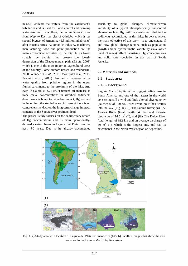
Annexes
217
m.a.s.l.) collects the waters from the catchment’s tributaries and is used for flood control and drinking water reservoir. Downflow, the Suquía River crosses from West to East the city of Córdoba which is the second biggest of Argentina (1.3 million inhabitants) after Buenos Aires. Automobile industry, machinery manufacturing, food and paint production are the main economical activities in the city. In its lower stretch, the Suquía river crosses the loessic depression of the Chacopampean plain (Zárate, 2003) which is one of the most important agricultural areas of the country. Some authors (Pesce and Wunderlin, 2000; Wunderlin et al., 2001; Monferrán et al, 2011, Pasquini et al., 2011) observed a decrease in the water quality from pristine regions in the upper fluvial catchments to the proximity of the lake. And even if Gaiero et al. (1997) noticed an increase in trace metal concentrations in riverbed sediments downflow attributed to the urban impact, Hg was not included into the studied ones. At present there is no comprehensive data on the long-term change in metal contents of the Suquía river sediment load. The present study focuses on the sedimentary record of Hg concentrations and its main operationally-defined carrier phases in Laguna del Plata over the past ~80 years. Due to its already documented
sensibility to global changes, climatic-driven variability of a typical atmospherically transported element such as Hg, will be clearly recorded in the sediments accumulated in this lake. In consequence, the main objective of this work is to understand if and how global change factors, such as population growth and/or hydroclimatic variability (lake-water level changes) affect lacustrine Hg concentrations and solid state speciation in this part of South America.
2 - Materials and methods
2.1 – Study area
2.1.1 – Background
Laguna Mar Chiquita is the biggest saline lake in South America and one of the largest in the world conserving still a wild and little altered physiognomy (Bucher et al., 2006). Three rivers pour their waters into the lake (Fig. 1a): (i) The Suquía River; (ii) The Xanaes River (total length 340 km and average discharge of 14.5 m3 s-1); and (iii) The Dulce River (total length of 812 km and an average discharge of 80 m3 s-1), which is the biggest one, and has its catchments in the North-West region of Argentina.
Fig. 1. a) Study area with location of Laguna del Plata sediment core (LP), b) Satellite images that show the size
variation in the Laguna Mar Chiquita system.
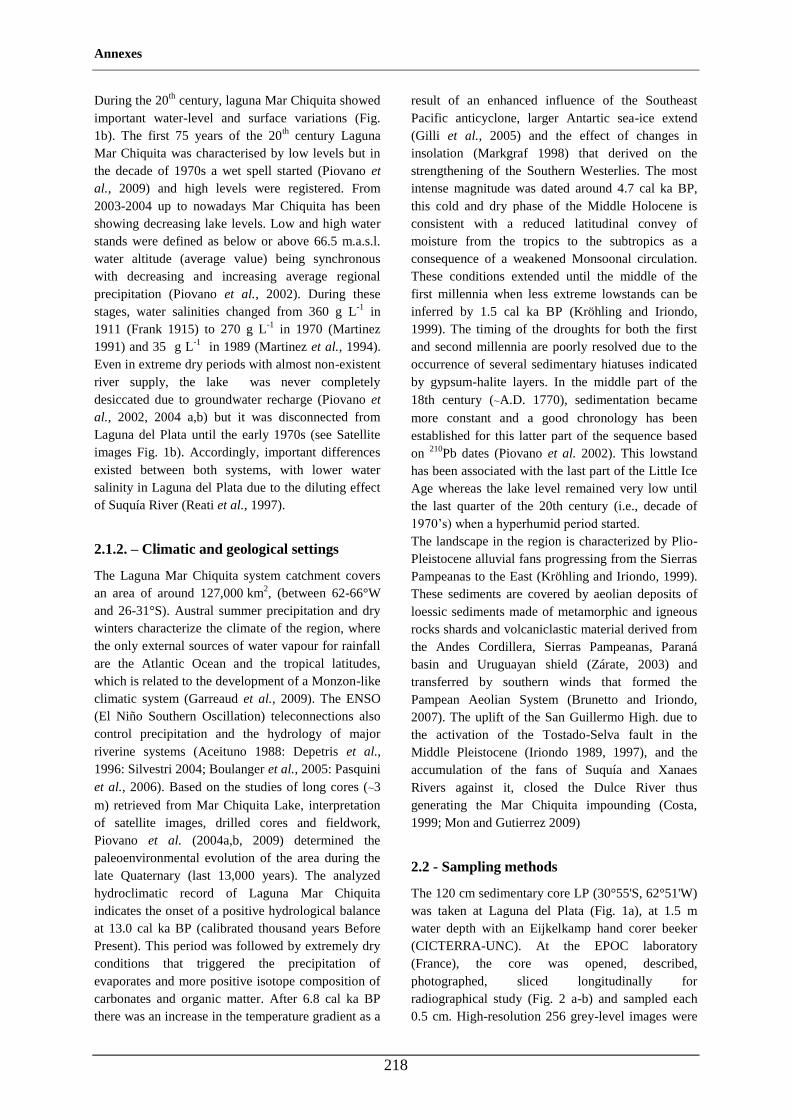
Annexes
218
During the 20th century, laguna Mar Chiquita showed important water-level and surface variations (Fig. 1b). The first 75 years of the 20th century Laguna Mar Chiquita was characterised by low levels but in the decade of 1970s a wet spell started (Piovano et al., 2009) and high levels were registered. From 2003-2004 up to nowadays Mar Chiquita has been showing decreasing lake levels. Low and high water stands were defined as below or above 66.5 m.a.s.l. water altitude (average value) being synchronous with decreasing and increasing average regional precipitation (Piovano et al., 2002). During these stages, water salinities changed from 360 g L-1 in 1911 (Frank 1915) to 270 g L-1 in 1970 (Martinez 1991) and 35 g L-1 in 1989 (Martinez et al., 1994). Even in extreme dry periods with almost non-existent river supply, the lake was never completely desiccated due to groundwater recharge (Piovano et al., 2002, 2004 a,b) but it was disconnected from Laguna del Plata until the early 1970s (see Satellite images Fig. 1b). Accordingly, important differences existed between both systems, with lower water salinity in Laguna del Plata due to the diluting effect of Suquía River (Reati et al., 1997).
2.1.2. – Climatic and geological settings
The Laguna Mar Chiquita system catchment covers an area of around 127,000 km2, (between 62-66°W and 26-31°S). Austral summer precipitation and dry winters characterize the climate of the region, where the only external sources of water vapour for rainfall are the Atlantic Ocean and the tropical latitudes, which is related to the development of a Monzon-like climatic system (Garreaud et al., 2009). The ENSO (El Niño Southern Oscillation) teleconnections also control precipitation and the hydrology of major riverine systems (Aceituno 1988: Depetris et al., 1996: Silvestri 2004; Boulanger et al., 2005: Pasquini et al., 2006). Based on the studies of long cores (~3 m) retrieved from Mar Chiquita Lake, interpretation of satellite images, drilled cores and fieldwork, Piovano et al. (2004a,b, 2009) determined the paleoenvironmental evolution of the area during the late Quaternary (last 13,000 years). The analyzed hydroclimatic record of Laguna Mar Chiquita indicates the onset of a positive hydrological balance at 13.0 cal ka BP (calibrated thousand years Before Present). This period was followed by extremely dry conditions that triggered the precipitation of evaporates and more positive isotope composition of carbonates and organic matter. After 6.8 cal ka BP there was an increase in the temperature gradient as a
result of an enhanced influence of the Southeast Pacific anticyclone, larger Antartic sea-ice extend (Gilli et al., 2005) and the effect of changes in insolation (Markgraf 1998) that derived on the strengthening of the Southern Westerlies. The most intense magnitude was dated around 4.7 cal ka BP, this cold and dry phase of the Middle Holocene is consistent with a reduced latitudinal convey of moisture from the tropics to the subtropics as a consequence of a weakened Monsoonal circulation. These conditions extended until the middle of the first millennia when less extreme lowstands can be inferred by 1.5 cal ka BP (Kröhling and Iriondo, 1999). The timing of the droughts for both the first and second millennia are poorly resolved due to the occurrence of several sedimentary hiatuses indicated by gypsum-halite layers. In the middle part of the 18th century (~A.D. 1770), sedimentation became more constant and a good chronology has been established for this latter part of the sequence based on 210Pb dates (Piovano et al. 2002). This lowstand has been associated with the last part of the Little Ice Age whereas the lake level remained very low until the last quarter of the 20th century (i.e., decade of 1970’s) when a hyperhumid period started. The landscape in the region is characterized by Plio-Pleistocene alluvial fans progressing from the Sierras Pampeanas to the East (Kröhling and Iriondo, 1999). These sediments are covered by aeolian deposits of loessic sediments made of metamorphic and igneous rocks shards and volcaniclastic material derived from the Andes Cordillera, Sierras Pampeanas, Paraná basin and Uruguayan shield (Zárate, 2003) and transferred by southern winds that formed the Pampean Aeolian System (Brunetto and Iriondo, 2007). The uplift of the San Guillermo High. due to the activation of the Tostado-Selva fault in the Middle Pleistocene (Iriondo 1989, 1997), and the accumulation of the fans of Suquía and Xanaes Rivers against it, closed the Dulce River thus generating the Mar Chiquita impounding (Costa, 1999; Mon and Gutierrez 2009)
2.2 - Sampling methods
The 120 cm sedimentary core LP (30°55'S, 62°51'W) was taken at Laguna del Plata (Fig. 1a), at 1.5 m water depth with an Eijkelkamp hand corer beeker (CICTERRA-UNC). At the EPOC laboratory (France), the core was opened, described, photographed, sliced longitudinally for radiographical study (Fig. 2 a-b) and sampled each 0.5 cm. High-resolution 256 grey-level images were
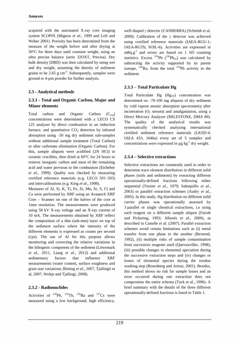
Annexes
219
acquired with the automated X-ray core imaging system SCOPIX (Migeon et al., 1999 and Lofi and Weber 2001). Porosity has been determined from the measure of the weight before and after drying at 50°C for three days until constant weight, using an ultra precise balance (serie 32OXT, Precisa). Dry bulk density (DBD) was then calculated by using wet and dry weight, assuming the density of sediment grains to be 2.65 g cm-3. Subsequently, samples were ground to 4-µm powder for further analysis.
2.3 - Analytical methods
2.3.1 - Total and Organic Carbon, Major and Minor elements
Total carbon and Organic Carbon (Corg) concentrations were determined with a LECO CS 125 analyzer by direct combustion in an induction furnace, and quantitative CO2 detection by infrared absorption using ~50 mg dry sediment sub-samples without additional sample treatment (Total Carbon) or after carbonate elimination (Organic Carbon). For this, sample aliquots were acidified (2N HCl) in ceramic crucibles, then dried at 60°C for 24 hours to remove inorganic carbon and most of the remaining acid and water previous to the combustion (Etcheber et al., 1999). Quality was checked by measuring certified reference materials (e.g. LECO 501–503) and intercalibrations (e.g. King et al., 1998). Measures of Al, Si, K, Ti, Fe, Zr, Mn, Sr, S, Cl and Ca were performed by XRF using an Avaatech XRF Core – Scanner on one of the halves of the core at 1mm resolution. The measurements were produced using 58 kV X-ray voltage and an X-ray current of 10 mA. The measurements obtained by XRF reflect the composition of a thin (sub-mm) layer on top of the sediment surface where the intensity of the different elements is expressed as counts per second (cps). The use of Al for this purpose allows monitoring and correcting the relative variations in the lithogenic component of the sediment (Löwemark et al., 2011, Liang et al., 2012) and additional sedimentary factors that influence XRF measurements (water content, surface roughness and grain size variations; Böning et al., 2007, Tjallingii et al, 2007; Weltje and Tjallingi, 2008).
2.3.2 - Radionuclides
Activities of 210Pb, 232Th, 226Ra and 137Cs were measured using a low background, high efficiency,
well-shaped detector (CANBERRA) (Schmidt et al,
2009). Calibration of the detector was achieved using certified reference materials (IAEA-RGU-1; IAEA-RGTh; SOIL-6). Activities are expressed in mBq.g-1 and errors are based on 1 SD counting statistics. Excess 210Pb (210Pbxs) was calculated by subtracting the activity supported by its parent isotope, 226Ra, from the total 210Pb activity in the sediment.
2.3.3 – Total Particulate Hg
Total Particulate Hg (HgTP) concentration was determined on ~70-100 mg aliquots of dry sediment by cold vapour atomic absorption spectrometry after incineration (O2 stream) and amalgamation, using a Direct Mercury Analyzer (MILESTONE, DMA 80). The quality of the analytical results was systematically checked analyzing international certified sediment reference materials (LKSD-4, IAEA 433, 1646a) every set of 5 samples and concentrations were expressed in µg kg-1 dry weight.
2.3.4 – Selective extractions
Selective extractions are commonly used in order to determine trace element distribution in different solid phases (soils and sediments) by extracting different operationally-defined fractions following either sequential (Tessier et al., 1979; Sahuquillo et al., 2003) or parallel extraction schemes (Audry et al., 2005). In this study, Hg distribution on different solid carrier phases was operationally assessed by 3 parallel or single chemical extractions, i.e using each reagent on a different sample aliquot (Farrah and Pickering, 1993; Alborés et al., 2000), as described in Castelle et al. (2007). Parallel extraction schemes avoid certain limitations such as (i) metal transfer from one phase to the another (Bemond, 1992), (ii) multiple risks of sample contamination from successive reagents used (Quevauviller, 1998), (iii) possible changes in elemental speciation during the successive extraction steps and (iv) changes or losses of elemental species during the residue washing step (Rosenberg and Ariese, 2001). Besides, this method shows no risk for sample losses and an error occurred during one extraction does not compromise the entire schema (Tack et al., 1996). A brief summary with the details of the three different operationally-defined fractions is listed in Table 1.
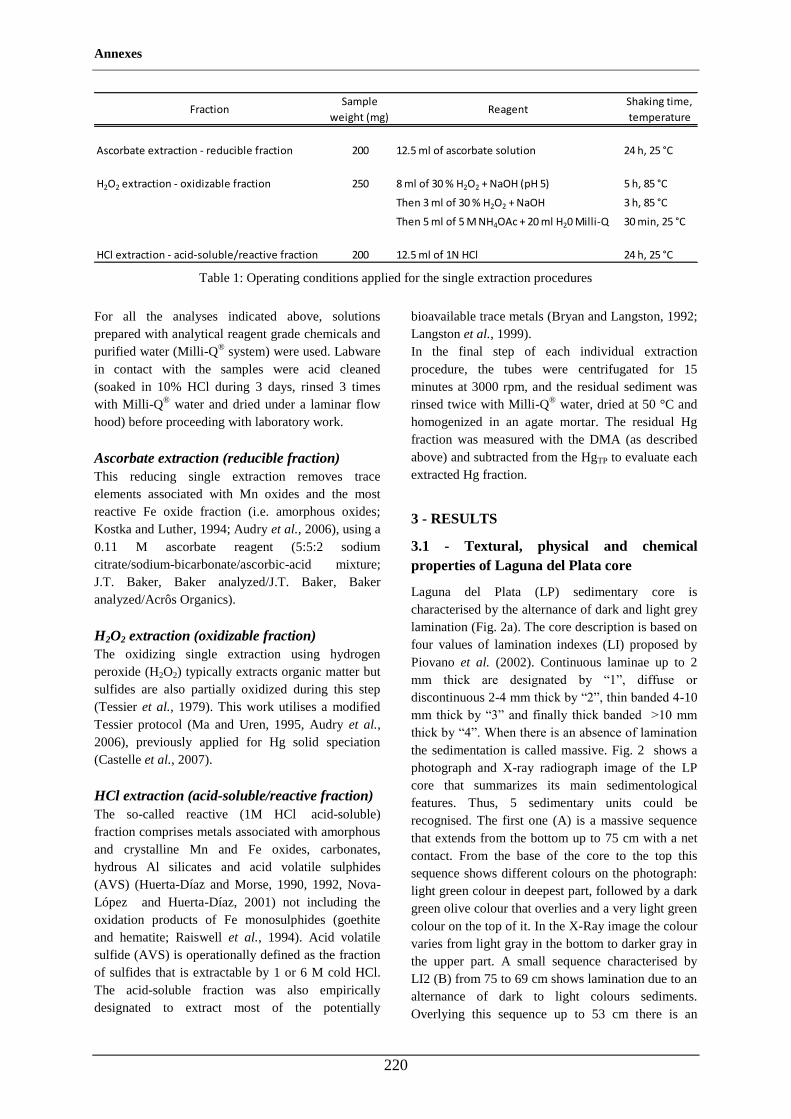
Annexes
220
Table 1: Operating conditions applied for the single extraction procedures
For all the analyses indicated above, solutions prepared with analytical reagent grade chemicals and purified water (Milli-Q® system) were used. Labware in contact with the samples were acid cleaned (soaked in 10% HCl during 3 days, rinsed 3 times with Milli-Q ® water and dried under a laminar flow hood) before proceeding with laboratory work.
Ascorbate extraction (reducible fraction) This reducing single extraction removes trace elements associated with Mn oxides and the most reactive Fe oxide fraction (i.e. amorphous oxides; Kostka and Luther, 1994; Audry et al., 2006), using a 0.11 M ascorbate reagent (5:5:2 sodium citrate/sodium-bicarbonate/ascorbic-acid mixture; J.T. Baker, Baker analyzed/J.T. Baker, Baker analyzed/Acrôs Organics).
H2O2 extraction (oxidizable fraction) The oxidizing single extraction using hydrogen peroxide (H2O2) typically extracts organic matter but sulfides are also partially oxidized during this step (Tessier et al., 1979). This work utilises a modified Tessier protocol (Ma and Uren, 1995, Audry et al., 2006), previously applied for Hg solid speciation (Castelle et al., 2007).
HCl extraction (acid-soluble/reactive fraction) The so-called reactive (1M HCl acid-soluble) fraction comprises metals associated with amorphous and crystalline Mn and Fe oxides, carbonates, hydrous Al silicates and acid volatile sulphides (AVS) (Huerta-Díaz and Morse, 1990, 1992, Nova-López and Huerta-Díaz, 2001) not including the oxidation products of Fe monosulphides (goethite and hematite; Raiswell et al., 1994). Acid volatile sulfide (AVS) is operationally defined as the fraction of sulfides that is extractable by 1 or 6 M cold HCl. The acid-soluble fraction was also empirically designated to extract most of the potentially
bioavailable trace metals (Bryan and Langston, 1992; Langston et al., 1999). In the final step of each individual extraction procedure, the tubes were centrifugated for 15 minutes at 3000 rpm, and the residual sediment was rinsed twice with Milli-Q® water, dried at 50 °C and homogenized in an agate mortar. The residual Hg fraction was measured with the DMA (as described above) and subtracted from the HgTP to evaluate each extracted Hg fraction.
3 - RESULTS
3.1 - Textural, physical and chemical properties of Laguna del Plata core
Laguna del Plata (LP) sedimentary core is characterised by the alternance of dark and light grey lamination (Fig. 2a). The core description is based on four values of lamination indexes (LI) proposed by Piovano et al. (2002). Continuous laminae up to 2 mm thick are designated by “1”, diffuse or discontinuous 2-4 mm thick by “2”, thin banded 4-10 mm thick by “3” and finally thick banded >10 mm thick by “4”. When there is an absence of lamination the sedimentation is called massive. Fig. 2 shows a photograph and X-ray radiograph image of the LP core that summarizes its main sedimentological features. Thus, 5 sedimentary units could be recognised. The first one (A) is a massive sequence that extends from the bottom up to 75 cm with a net contact. From the base of the core to the top this sequence shows different colours on the photograph: light green colour in deepest part, followed by a dark green olive colour that overlies and a very light green colour on the top of it. In the X-Ray image the colour varies from light gray in the bottom to darker gray in the upper part. A small sequence characterised by LI2 (B) from 75 to 69 cm shows lamination due to an alternance of dark to light colours sediments. Overlying this sequence up to 53 cm there is an
FractionSample
weight (mg)Reagent
Shaking time,
temperature
Ascorbate extraction - reducible fraction 200 12.5 ml of ascorbate solution 24 h, 25 °C
H2O2 extraction - oxidizable fraction 250 8 ml of 30 % H2O2 + NaOH (pH 5) 5 h, 85 °C
Then 3 ml of 30 % H2O2 + NaOH 3 h, 85 °C
Then 5 ml of 5 M NH4OAc + 20 ml H20 Milli-Q 30 min, 25 °C
HCl extraction - acid-soluble/reactive fraction 200 12.5 ml of 1N HCl 24 h, 25 °C
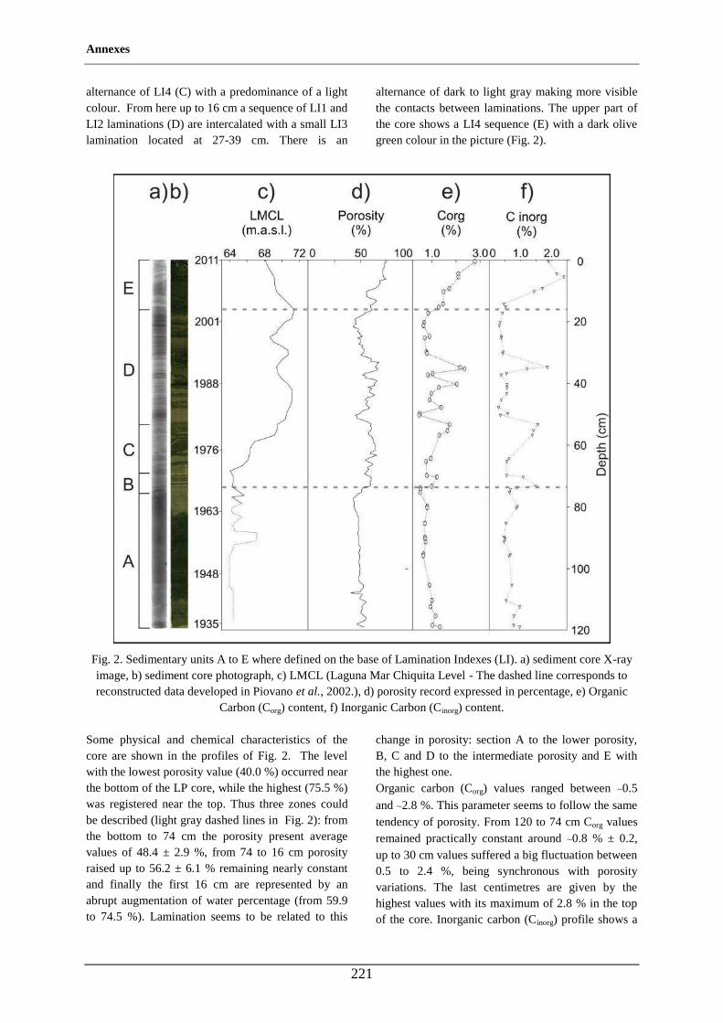
Annexes
221
alternance of LI4 (C) with a predominance of a light colour. From here up to 16 cm a sequence of LI1 and LI2 laminations (D) are intercalated with a small LI3 lamination located at 27-39 cm. There is an
alternance of dark to light gray making more visible the contacts between laminations. The upper part of the core shows a LI4 sequence (E) with a dark olive green colour in the picture (Fig. 2).
Fig. 2. Sedimentary units A to E where defined on the base of Lamination Indexes (LI). a) sediment core X-ray image, b) sediment core photograph, c) LMCL (Laguna Mar Chiquita Level - The dashed line corresponds to reconstructed data developed in Piovano et al., 2002.), d) porosity record expressed in percentage, e) Organic
Carbon (Corg) content, f) Inorganic Carbon (Cinorg) content. Some physical and chemical characteristics of the core are shown in the profiles of Fig. 2. The level with the lowest porosity value (40.0 %) occurred near the bottom of the LP core, while the highest (75.5 %) was registered near the top. Thus three zones could be described (light gray dashed lines in Fig. 2): from the bottom to 74 cm the porosity present average values of 48.4 ± 2.9 %, from 74 to 16 cm porosity raised up to 56.2 ± 6.1 % remaining nearly constant and finally the first 16 cm are represented by an abrupt augmentation of water percentage (from 59.9 to 74.5 %). Lamination seems to be related to this
change in porosity: section A to the lower porosity, B, C and D to the intermediate porosity and E with the highest one. Organic carbon (Corg) values ranged between ~0.5
and ~2.8 %. This parameter seems to follow the same tendency of porosity. From 120 to 74 cm Corg values remained practically constant around ~0.8 % ± 0.2, up to 30 cm values suffered a big fluctuation between 0.5 to 2.4 %, being synchronous with porosity variations. The last centimetres are given by the highest values with its maximum of 2.8 % in the top of the core. Inorganic carbon (Cinorg) profile shows a
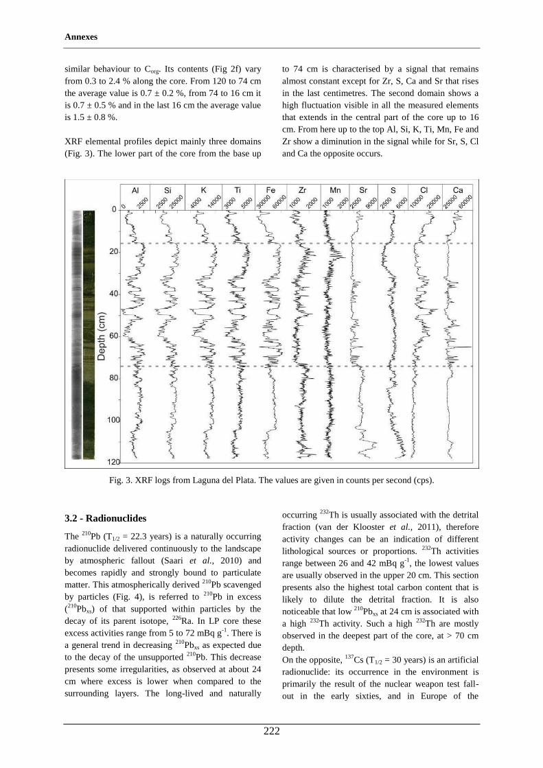
Annexes
222
similar behaviour to Corg. Its contents (Fig 2f) vary from 0.3 to 2.4 % along the core. From 120 to 74 cm the average value is 0.7 ± 0.2 %, from 74 to 16 cm it is 0.7 ± 0.5 % and in the last 16 cm the average value is 1.5 ± 0.8 %. XRF elemental profiles depict mainly three domains (Fig. 3). The lower part of the core from the base up
to 74 cm is characterised by a signal that remains almost constant except for Zr, S, Ca and Sr that rises in the last centimetres. The second domain shows a high fluctuation visible in all the measured elements that extends in the central part of the core up to 16 cm. From here up to the top Al, Si, K, Ti, Mn, Fe and Zr show a diminution in the signal while for Sr, S, Cl and Ca the opposite occurs.
Fig. 3. XRF logs from Laguna del Plata. The values are given in counts per second (cps).
3.2 - Radionuclides
The 210Pb (T1/2 = 22.3 years) is a naturally occurring radionuclide delivered continuously to the landscape by atmospheric fallout (Saari et al., 2010) and becomes rapidly and strongly bound to particulate matter. This atmospherically derived 210Pb scavenged by particles (Fig. 4), is referred to 210Pb in excess (210Pbxs) of that supported within particles by the decay of its parent isotope, 226Ra. In LP core these excess activities range from 5 to 72 mBq g-1. There is a general trend in decreasing 210Pbxs as expected due to the decay of the unsupported 210Pb. This decrease presents some irregularities, as observed at about 24 cm where excess is lower when compared to the surrounding layers. The long-lived and naturally
occurring 232Th is usually associated with the detrital fraction (van der Klooster et al., 2011), therefore activity changes can be an indication of different lithological sources or proportions. 232Th activities range between 26 and 42 mBq g-1, the lowest values are usually observed in the upper 20 cm. This section presents also the highest total carbon content that is likely to dilute the detrital fraction. It is also noticeable that low 210Pbxs at 24 cm is associated with a high 232Th activity. Such a high 232Th are mostly observed in the deepest part of the core, at > 70 cm depth. On the opposite, 137Cs (T1/2 = 30 years) is an artificial radionuclide: its occurrence in the environment is primarily the result of the nuclear weapon test fall-out in the early sixties, and in Europe of the
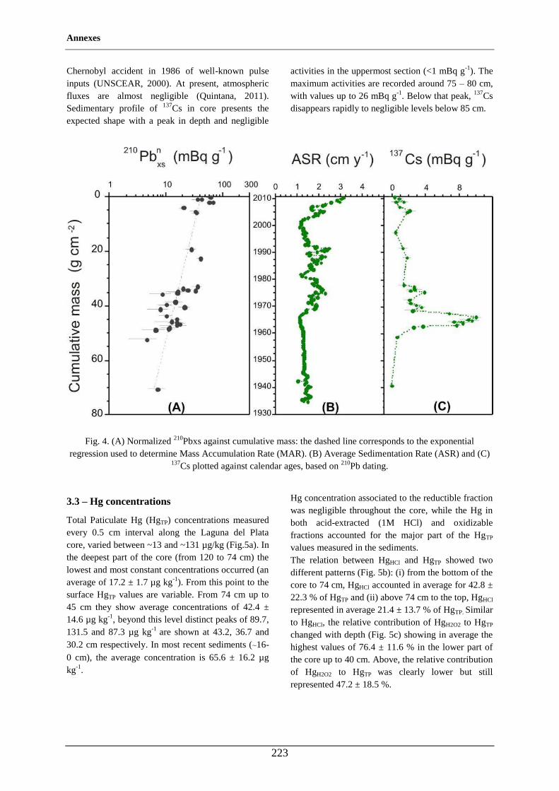
Annexes
223
Chernobyl accident in 1986 of well-known pulse inputs (UNSCEAR, 2000). At present, atmospheric fluxes are almost negligible (Quintana, 2011). Sedimentary profile of 137Cs in core presents the expected shape with a peak in depth and negligible
activities in the uppermost section (<1 mBq g-1). The maximum activities are recorded around 75 – 80 cm, with values up to 26 mBq g-1. Below that peak, 137Cs disappears rapidly to negligible levels below 85 cm.
Fig. 4. (A) Normalized 210Pbxs against cumulative mass: the dashed line corresponds to the exponential
regression used to determine Mass Accumulation Rate (MAR). (B) Average Sedimentation Rate (ASR) and (C) 137Cs plotted against calendar ages, based on 210Pb dating.
3.3 – Hg concentrations
Total Paticulate Hg (HgTP) concentrations measured every 0.5 cm interval along the Laguna del Plata core, varied between ~13 and ~131 µg/kg (Fig.5a). In the deepest part of the core (from 120 to 74 cm) the lowest and most constant concentrations occurred (an average of 17.2 ± 1.7 µg kg-1). From this point to the surface HgTP values are variable. From 74 cm up to 45 cm they show average concentrations of 42.4 ± 14.6 µg kg-1, beyond this level distinct peaks of 89.7, 131.5 and 87.3 µg kg-1 are shown at 43.2, 36.7 and 30.2 cm respectively. In most recent sediments (~16-0 cm), the average concentration is 65.6 ± 16.2 µg kg-1.
Hg concentration associated to the reductible fraction was negligible throughout the core, while the Hg in both acid-extracted (1M HCl) and oxidizable fractions accounted for the major part of the HgTP values measured in the sediments. The relation between HgHCl and HgTP showed two different patterns (Fig. 5b): (i) from the bottom of the core to 74 cm, HgHCl accounted in average for 42.8 ± 22.3 % of HgTP and (ii) above 74 cm to the top, HgHCl represented in average 21.4 ± 13.7 % of HgTP. Similar to HgHCl, the relative contribution of HgH2O2 to HgTP
changed with depth (Fig. 5c) showing in average the highest values of 76.4 ± 11.6 % in the lower part of the core up to 40 cm. Above, the relative contribution of HgH2O2 to HgTP was clearly lower but still represented 47.2 ± 18.5 %.
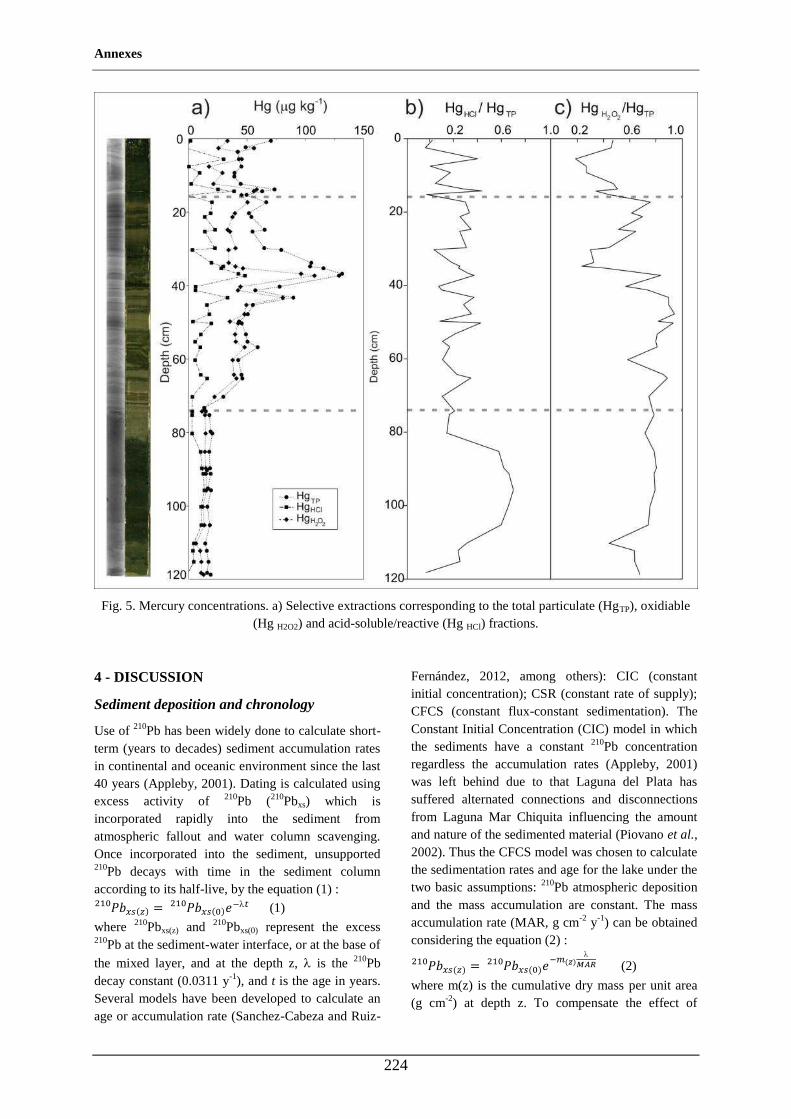
Annexes
224
Fig. 5. Mercury concentrations. a) Selective extractions corresponding to the total particulate (HgTP), oxidiable
(Hg H2O2) and acid-soluble/reactive (Hg HCl) fractions.
4 - DISCUSSION
Sediment deposition and chronology
Use of 210Pb has been widely done to calculate short-term (years to decades) sediment accumulation rates in continental and oceanic environment since the last 40 years (Appleby, 2001). Dating is calculated using excess activity of 210Pb (210Pbxs) which is incorporated rapidly into the sediment from atmospheric fallout and water column scavenging. Once incorporated into the sediment, unsupported 210Pb decays with time in the sediment column according to its half-live, by the equation (1) : (1)
where 210Pbxs(z) and 210Pbxs(0) represent the excess 210Pb at the sediment-water interface, or at the base of
the mixed layer, and at the depth z, is the 210Pb decay constant (0.0311 y-1), and t is the age in years. Several models have been developed to calculate an age or accumulation rate (Sanchez-Cabeza and Ruiz-
Fernández, 2012, among others): CIC (constant initial concentration); CSR (constant rate of supply); CFCS (constant flux-constant sedimentation). The Constant Initial Concentration (CIC) model in which the sediments have a constant 210Pb concentration regardless the accumulation rates (Appleby, 2001) was left behind due to that Laguna del Plata has suffered alternated connections and disconnections from Laguna Mar Chiquita influencing the amount and nature of the sedimented material (Piovano et al., 2002). Thus the CFCS model was chosen to calculate the sedimentation rates and age for the lake under the two basic assumptions: 210Pb atmospheric deposition and the mass accumulation are constant. The mass accumulation rate (MAR, g cm-2 y-1) can be obtained considering the equation (2) : (2)
where m(z) is the cumulative dry mass per unit area (g cm-2) at depth z. To compensate the effect of
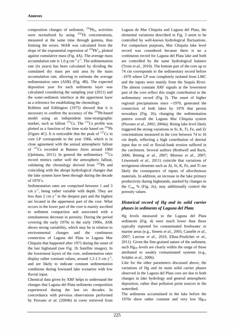
Annexes
225
composition changes of sediment, 210Pbxs activities were normalized by using 232Th concentrations, measured at the same time through gamma, thus limiting the errors. MAR was calculated from the slope of the exponential regression of 210Pbn
xs plotted against cumulative mass (Fig. 4A). The average mass accumulation rate is 1.0 g cm-2 y-1. The sedimentation rate (in years) has been calculated by dividing the cumulated dry mass per unit area by the mass accumulation rate, allowing to estimate the average sedimentation rates (ASR) (Fig. 4B). The expected deposition year for each sediments layer was calculated considering the sampling year (2011) and the water-sediment interface at the uppermost layer as a reference for establishing the chronology. Robbins and Eddington (1975) showed that it is necessary to confirm the accuracy of the 210Pb-based model using an independent time-stratigraphic marker, such as fallout 137Cs. The 137Cs profile was plotted as a function of the time scale based on 210Pb (Figure 4C). It is noticeable that the peak of 137Cs in core LP corresponds to the year 1966, which is in close agreement with the annual atmospheric fallout of 137Cs recorded at Buenos Aires around 1960 (Quintana, 2011). In general the sedimentary 137Cs record mimics rather well the atmospheric fallout, validating the chronology derived from 210Pb and coinciding with the abrupt hydrological changes that the lake system have been through during the decade of 1970’s. Sedimentation rates are comprised between 1 and 3 cm y-1, being rather variable with depth. They are less than 2 cm y-1 in the deepest part and the highest are located in the uppermost part of the core. What occurs in the lower part of the core is mainly ascribed to sediment compaction and associated with a simultaneous decrease in porosity. During the period covering the early 1970s to the early 1990s, ASR shows strong variability, which may be in relation to environmental changes and the continuous connection of Laguna del Plata to Laguna Mar Chiquita that happened after 1975 during the onset of the last highstand (see Fig. 1b Satellite images). In the lowermost layers of the core, sedimentation rates display rather constant values, around 1.2-1.5 cm y-1, and are likely to indicate constant sedimentation conditions during lowstand lake scenarios with low fluvial input. Chemical data given by XRF helps to understand the changes that Laguna del Plata sediments composition experienced during the last six decades. In concordance with previous observations performed by Piovano et al. (2004b) in cores retrieved from
Laguna de Mar Chiquita and Laguna del Plata, the elemental variations described in Fig. 3 seem to be controlled by well-known hydrological fluctuations. For comparison purposes, Mar Chiquita lake level record was considered because there is no a continuous record for Laguna del Plata lake and both are controlled by the same hydrological balance (Troin et al., 2010). The bottom part of the core up to 74 cm corresponds to the sedimentary record before ~1970 where LP was completely isolated from LMC and the inputs were mainly from the Suquía River. The almost constant XRF signals at the lowermost part of the core reflect this single contribution to the sedimentary record (Fig 3). The onset of higher
regional precipitations since 1970, generated the connection of both lakes by 1976 that persist nowadays (Fig. 1b), changing the sedimentation pattern overall the Laguna Mar Chiquita system (Piovano et al., 2002; 2004a). Rising lake level likely triggered the strong variations in Si, K, Ti, Fe, and Zr concentations measured in the core between 74 to 16 cm depth, reflecting a high contribution of detrital input due to soil or fluvial-bank erosion suffered in the catchment. Several authors (Rothwell and Rack, 2006; Böning et al., 2007; Moreno et al., 2007; Löwemark et al., 2011) coincide that variations of terrigenous elements such as Al, Si, K, Fe, and Ti are likely the consequence of inputs of allocthonous materials. In addition, an increase in the lake primary productivity during highstands, marked by changes in the Corg % (Fig. 2e), may additionally control the porosity values.
Historical record of Hg and its solid carrier phases in sediments of Laguna del Plata
Hg levels measured in the Laguna del Plata sediments (Fig. 4) were much lower than those typically reported for contaminated freshwater or marine areas (e.g., Streets et al., 2005; Castelle et al., 2007; Larrose et al., 2010, Elbaz-Poulichet et al., 2011). Given the fine-grained nature of the sediment, such HgTP levels are clearly within the range of those attributed to weakly contaminated systems (e.g., Schäfer et al., 2006). Like for the other parameters discussed above, the variations of Hg and its main solid carrier phases observed in the Laguna del Plata core are due to both changes in lake hydrology and general atmospheric deposition, rather than pollution point sources in the watershed. The sediments accumulated in the lake before the 1970s show rather constant and very low HgTP
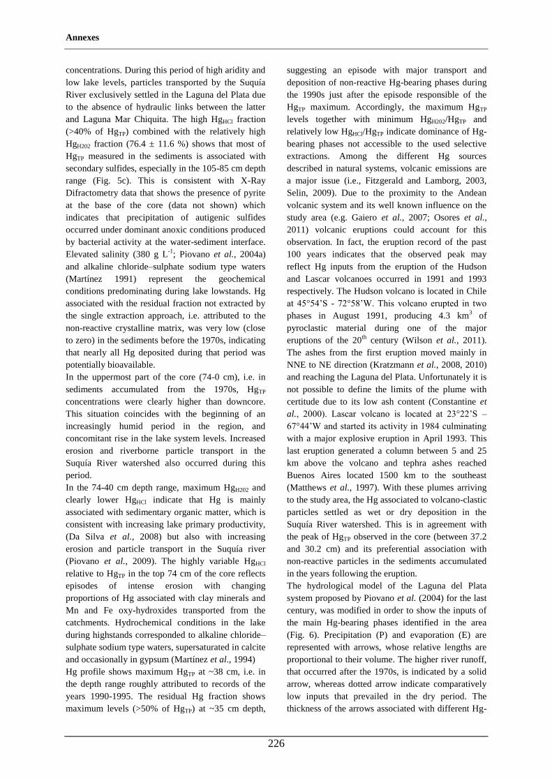
Annexes
226
concentrations. During this period of high aridity and low lake levels, particles transported by the Suquía River exclusively settled in the Laguna del Plata due to the absence of hydraulic links between the latter and Laguna Mar Chiquita. The high HgHCl fraction (>40% of HgTP) combined with the relatively high HgH202 fraction (76.4 ± 11.6 %) shows that most of HgTP measured in the sediments is associated with secondary sulfides, especially in the 105-85 cm depth range (Fig. 5c). This is consistent with X-Ray Difractometry data that shows the presence of pyrite at the base of the core (data not shown) which indicates that precipitation of autigenic sulfides occurred under dominant anoxic conditions produced by bacterial activity at the water-sediment interface. Elevated salinity (380 g L-1; Piovano et al., 2004a) and alkaline chloride–sulphate sodium type waters (Martínez 1991) represent the geochemical conditions predominating during lake lowstands. Hg associated with the residual fraction not extracted by the single extraction approach, i.e. attributed to the non-reactive crystalline matrix, was very low (close to zero) in the sediments before the 1970s, indicating that nearly all Hg deposited during that period was potentially bioavailable. In the uppermost part of the core (74-0 cm), i.e. in sediments accumulated from the 1970s, HgTP concentrations were clearly higher than downcore. This situation coincides with the beginning of an increasingly humid period in the region, and concomitant rise in the lake system levels. Increased erosion and riverborne particle transport in the Suquía River watershed also occurred during this period. In the 74-40 cm depth range, maximum HgH202 and clearly lower HgHCl indicate that Hg is mainly associated with sedimentary organic matter, which is consistent with increasing lake primary productivity, (Da Silva et al., 2008) but also with increasing erosion and particle transport in the Suquía river (Piovano et al., 2009). The highly variable HgHCl relative to HgTP in the top 74 cm of the core reflects episodes of intense erosion with changing proportions of Hg associated with clay minerals and Mn and Fe oxy-hydroxides transported from the catchments. Hydrochemical conditions in the lake during highstands corresponded to alkaline chloride–sulphate sodium type waters, supersaturated in calcite and occasionally in gypsum (Martínez et al., 1994) Hg profile shows maximum HgTP at ~38 cm, i.e. in the depth range roughly attributed to records of the years 1990-1995. The residual Hg fraction shows maximum levels (>50% of HgTP) at ~35 cm depth,
suggesting an episode with major transport and deposition of non-reactive Hg-bearing phases during the 1990s just after the episode responsible of the HgTP maximum. Accordingly, the maximum HgTP levels together with minimum HgH202/HgTP and relatively low HgHCl/HgTP indicate dominance of Hg-bearing phases not accessible to the used selective extractions. Among the different Hg sources described in natural systems, volcanic emissions are a major issue (i.e., Fitzgerald and Lamborg, 2003, Selin, 2009). Due to the proximity to the Andean volcanic system and its well known influence on the study area (e.g. Gaiero et al., 2007; Osores et al., 2011) volcanic eruptions could account for this observation. In fact, the eruption record of the past 100 years indicates that the observed peak may reflect Hg inputs from the eruption of the Hudson and Lascar volcanoes occurred in 1991 and 1993 respectively. The Hudson volcano is located in Chile at 45°54’S - 72°58’W. This volcano erupted in two phases in August 1991, producing 4.3 km3 of pyroclastic material during one of the major eruptions of the 20th century (Wilson et al., 2011). The ashes from the first eruption moved mainly in NNE to NE direction (Kratzmann et al., 2008, 2010) and reaching the Laguna del Plata. Unfortunately it is not possible to define the limits of the plume with certitude due to its low ash content (Constantine et al., 2000). Lascar volcano is located at 23°22’S – 67°44’W and started its activity in 1984 culminating with a major explosive eruption in April 1993. This last eruption generated a column between 5 and 25 km above the volcano and tephra ashes reached Buenos Aires located 1500 km to the southeast (Matthews et al., 1997). With these plumes arriving to the study area, the Hg associated to volcano-clastic particles settled as wet or dry deposition in the Suquía River watershed. This is in agreement with the peak of HgTP observed in the core (between 37.2 and 30.2 cm) and its preferential association with non-reactive particles in the sediments accumulated in the years following the eruption. The hydrological model of the Laguna del Plata system proposed by Piovano et al. (2004) for the last century, was modified in order to show the inputs of the main Hg-bearing phases identified in the area (Fig. 6). Precipitation (P) and evaporation (E) are represented with arrows, whose relative lengths are proportional to their volume. The higher river runoff, that occurred after the 1970s, is indicated by a solid arrow, whereas dotted arrow indicate comparatively low inputs that prevailed in the dry period. The thickness of the arrows associated with different Hg-
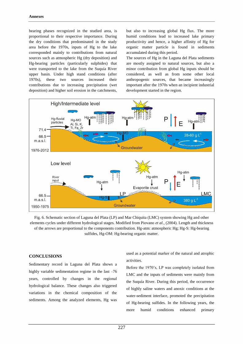
Annexes
227
bearing phases recognized in the studied area, is proportional to their respective importance. During the dry conditions that predominated in the study area before the 1970s, inputs of Hg to the lake corresponded mainly to contributions from natural sources such as atmospheric Hg (dry deposition) and Hg-bearing particles (particularly sulphides) that were transported to the lake from the Suquía River upper basin. Under high stand conditions (after 1970s), these two sources increased their contributions due to increasing precipitation (wet deposition) and higher soil erosion in the catchments,
but also to increasing global Hg flux. The more humid conditions lead to increased lake primary productivity and hence, a higher affinity of Hg for organic matter particle is found in sediments accumulated during this period. The sources of Hg in the Laguna del Plata sediments are mostly assigned to natural sources, but also a minor contribution from global Hg inputs should be considered, as well as from some other local anthropogenic sources, that became increasingly important after the 1970s when an incipient industrial development started in the region.
Fig. 6. Schematic section of Laguna del Plata (LP) and Mar Chiquita (LMC) system showing Hg and other elements cycles under different hydrological stages. Modified from Piovano et al., (2004). Length and thickness
of the arrows are proportional to the components contribution. Hg-atm: atmospheric Hg; Hg-S: Hg-bearing sulfides, Hg-OM: Hg-bearing organic matter.
CONCLUSIONS
Sedimentary record in Laguna del Plata shows a
highly variable sedimentation regime in the last ~76
years, controlled by changes in the regional
hydrological balance. These changes also triggered
variations in the chemical composition of the
sediments. Among the analyzed elements, Hg was
used as a potential marker of the natural and atrophic
activities.
Before the 1970’s, LP was completely isolated from
LMC and the inputs of sediments were mainly from
the Suquía River. During this period, the occurrence
of highly saline waters and anoxic conditions at the
water-sediment interface, promoted the precipitation
of Hg-bearing sulfides. In the following years, the
more humid conditions enhanced primary
Annexes
228
productivity in the lake, driving increased organic
matter contents in the sediment record. Hg
accumulated during this period, was preferentially
associated with the organic fraction of the sediments.
The upper centimetres of the core show increasing
Hg concentrations that are considered to be closely
related to the industrial development of the region
but also to the increasing influence of global Hg
fluxes.
The highest HgTP values are found at ~35 cm depth
(corresponding to the years 1990-1995) where the
HgH202/HgTP and HgHCl/HgTP relations are also
relatively low. This suggests a contribution from a
Hg-bearing source that is not affected by the applied
extraction methods. More than a punctual source of
pollution, this peak is likely related to two eruptive
events occurred in the Andean Cordillera in this
period: the eruption of Hudson volcano in southern
Patagonia that occurred in 1991 and the one of the
Lascar volcano in northern Chile that occurred in
1993. In both cases, the respective ash plumes were
documented to have reached the Laguna del Plata
region.
ACKNOWLEDGMENTS
This work is in the frame of a doctoral thesis
financed by ERASMUS MUNDUS External
Cooperation Window, lot 18 –BAPE – Bolivia,
Argentina, Peru and Europe. Field trips were
financed with funds from PIP 112-200801-00808
(CONICET-Argentina). The authors want to thank
equally to the reviewers and their constructive
remarks.
REFERENCES
Aceituno, P., 1988. On the functioning of the Southern
Oscillation in the South American sector. Part I: surface
climate. Monthly Weather Review. 116, 505–524.
Alborés, A.F., Cid, B.P., Gómez, E.F. and López, E.F.,
2000. Comparison between sequential extraction
procedures and single extractions for metal partitioning
in sewage sludge samples. Analyst. 125, 1353-1357.
Amin, O., Ferrer, L. and Marcovecchio, J., 1996. Heavy
metal concentrations in litteral sediments from the Beagle
Channel, Tierra del Fuego, Argentina. Environmental
Monitoring and Assessment 41 (3), 219-231.
Appleby, P.G., 2001. Chronostratigraphic techniques in
recent sediments. W. M. Last & J. P. Smol
(eds.).Tracking Environmental Change Using Lake
Sediments. Volume 1: Basin Analysis, Coring, and
Chronological Techniques. Kluwer Academic Publishers,
Dordrecht, The Netherlands.
Arribére, M.A., Ribeiro Guevara, S., Sánchez, R.S., Gil,
M.I., Román Ross, G., Daurade, L.E., Fajon, V., Horvat,
M., Alcalde, R. and Kestelman, A.J., 2003. Heavy metals
in the vicinity of a chlor-alkali factory in the upper Negro
River ecosystem, Northern Patagonia, Argentina. Science
of the Total Environment. 301 (1-3), 187-203.
Audry, S., Blanc, G. and Schäfer, J., 2005. The impact of
sulphide oxidation on dissolved metal (Cd, Zn, Cu, Cr,
Co, Ni, U) inputs into the Lot-Garonne fluvial system
(France). Applied Geochemistry 20 (5), 919-931.
Audry, S., Blanc, G., Schäfer, J., 2006. Solid state
partitioning of trace metals in suspended particulate
matter from a river system affected by smelting waste
drainage. Science of the Total Environment. 363, 216–
236.
Balcom, P., Fitzgerald, W., Hammerschmidt, C., Lamborg,
C, and Graham, L., 2004. Mercury sources and speciation
in the waters of New York/New Jersey Harbor Estuary.
Mater. Geoenviron. 51, 795–798. Environmental
Technology 13 (12), 1175-1179.
Bermond, A.P., 1992. Thermodynamics applied to the
study of the limits of sequential extraction procedures
used for the speciation of trace elements in sediments and
soils. Environmental Technology. 13 (12), 1175-1179.
Biester, H., Bindler, R., Martinez-Cortizas, A. and
Engstrom, D.R., 2007. Modeling the past atmospheric
deposition of mercury using natural archives.
Environmental Science and Technology. 41, 4851–4860.
Böning, P., Bard, E. and Rose, J., 2007. Toward direct,
micron-scale XRF elemental maps and quantitative
profiles of wet marine sediments. Geochemistry,
Geophysics, Geosystems. 8 (5),
doi:10.1029/2006GC001480.
Botté, S.E., Freije, R.H. and Marcovecchio, J.E., 2010.
Distribution of Several Heavy Metals in Tidal Flats
Annexes
229
Sediments within Bahía Blanca Estuary (Argentina).
Water Air Soil Pollution. 210, 371–388. DOI
10.1007/s11270-009-0260-0.
Boulanger, J-P., Leloup, J., Penalba, O., Rusticucci, M.,
Lafon, F. and Vargas, W., 2005. Observed precipitation
in the Paraná-Plata hydrological basin: long-term trends,
extreme conditions and ENSO teleconnections. Climate
Dynamics. 24, 393-413.
Brunetto, E. and Iriondo, M.H., 2007. Neotectónica en la
Pampa Norte (Argentina). Revista de la Sociedad
Geológica de España, 20 (1-2), 17-29.
Bryan, G.W. and Langston, W.J., 1992. Bioavailability,
accumulation and effects of heavy metals in sediments
with special reference to United Kingdom estuaries: a
review. Environmental Pollution. 76 (2), 89– 131.
Bucher, E.H., Gavier Pizarro, G. and Curto, E.D., 2006.
Cap. 1. Síntesis geográfica. En: Bañados del Río Dulce y
Mar Chiquita (Córdoba, Argentina) (ed. Bucher E.H), pp.
15-27. Academia Nacional de Ciencias (Córdoba,
Argentina).
Constantine, E.K., Bluth, G.J.S. and Rose, W.I., 2000.
TOMS and AVHRR Observations of Drifting Volcanic
Clouds From the August 1991 Eruptions of Cerro
Hudson. Mouginis-Mark, P., Crisp, J.A., Fink, J.H.
(Eds.), Remote Sensing of Active Volcanism.
Geophysical Monograph, Washington, DC, pp. 45–64.
Costa, C., 1999. Tectónica cuaternaria en las Sierras
Pampeanas. Geología Argentina. Anales 29.
Subsecretaría de Minería de la Nación. Servicio
Geológico Minero Argentino. Instituto de Geología y
Recursos Minerales. Buenos Aires.
Da Silva, L.S.V., Piovano, E.L., Azevedo, D.d.A., Aquino
Neto, F.R.d., 2008. Quantitative evaluation of
sedimentary organic matter from Laguna Mar Chiquita,
Argentina. Organic Geochemistry. 39 (4), 450-464.
De Marco, S.G., Botté, S.E. and Marcovecchio, J.E., 2006.
Mercury distribution in abiotic and biological
compartments within several estuarine systems from
Argentina: 1980–2005 period. Chemosphere. 65, 213–
223.
Depetris, P.J., Kempe, S., Latif, M. and Mook, W.G., 1996.
ENSO controlled flooding in the Paraná River (1904-
1991). Naturwissenschaften. 83, 127–129.
Diaz, E., 2000. Mercury pollution at gold mining sites in
the Amazon environment. Principles of Environmental
Toxicology. University of Idaho. pp. 24.
Downs, S. G., Macleod, C. L., and Lester, J. N., 1998.
Mercury in precipitation and its relation to
bioaccumulation in fish: a literature review. Water Air
and Soil Pollution. 108, 149–187.
Etcheber, H., Relexans, J-C., Beliard, M., Weber, O.,
Buscail, R. and Heussner, S., 1999. Distribution and
quality of sedimentary organic matter on the Aquitanian
margin (Bay of Biscay). Deep-Sea Research II. 46, 2249-
2288.
Elbaz-Poulichet, F., Dezileau, L., Freydier, R., Cossa, D.
and Sabatier, P., 2011. A 3500-year record of Hg and Pb
contamination in a mediterranean sedimentary archive
(The Pierre Blanche Lagoon, France). Environmental
Science and Technology. 45 (20), 8642-8647.
Farrah, H. and Pickering W.F., 1993. Factors influencing
the potential mobility and bioavailability of metals in
dried lake sediments. Chemical Speciation and
Bioavailability. 5 (3), 81-96.
Fitzgerald, W.F. and Mason, R.P., 1997. Biogeochemical
cycling of mercury in the marine environment. In: Sigel,
H., Sigel, A. (Eds.), Metal Ions in Biological Systems,
Mercury and its Effects on Environment and Biological
Systems, vol. 34. Marcel Dekker Inc., New York, pp. 3–
110.
Fitzgerald, W.F. and Lamborg C.H., 2003. Geochemistry
of Mercury in the Environment. In: In: Holland, H.D. and
Turekian, K.K. (Eds), Treatise on Geochemistry, ed. BS
Lollar, pp. 107-148. New York: Elsevier.
Frank, H., 1915. Contribución al conocimiento de las
Salinas Grandes y la Mar Chiquita de la Provincia de
Córdoba. Revista del Centro de Estudiantes de
Ingienería, 3:91-107.
Gagnon, C., Pelletier, É. and Mucchi, A., 1997. Behaviour
of anthropogenic mercury in coastal marine sediment.
Marine Chemistry. 59, 159-176.
Gaiero D.M., Roman Ross, G., Depetris, P.J. and Kempe,
S. 1997. Spatial and temporal variability of total non-
residual heavy metals content in stream sediments from
the Suquía river system, Córdooba, Argentina. Water, Air
and Soil pollution. 93, 303-319.
Gaiero D.M., Brunet, F., Probst, J-L. and Depetris, P.J.,
2007. A uniform isotopic and chemical signature of dust
Annexes
230
exported from Patagonia: Rock sources and occurrence in
southern environments. Chemical Geology. 238 (1-2),
107-120.
Garreaud, R.D., Vuille, M., Compagnucci, R. and
Marengo, J., 2009. Present-day Souh American Climate
(LOTRED South America). Palaeogeography,
Palaeoclimatology, Palaeoecology. 281, 180–195.
Gilli A., Anselmetti F.S. and Ariztegui D., 2005. Seismic
stratigraphy, buried beach ridges and contourite drifts:
The Late Quaternary history of the closed Lago Cardiel
basin, Argentina (49°S). Sedimentology. 51, 1–23.
Hermanns, Y.M. and Biester, H., 2013. Anthropogenic
mercury signals in lake sediments from southernmost
Patagonia, Chile. Science of the Total Environment. 445-
446, 126-135.
Hudson-Edwards, K.A., Macklin, M.G., Miller, J.R. and
Lechler, P.J., 2001. Sources, distribution and storage of
heavy metals in the Río Pilcomayo, Bolivia. Journal of
Geochemical Exploration. 72 (3), 229-250.
Huerta-Diaz, M.A. and Morse, J.W., 1990. A quantitative
method for determination of trace metal concentrations in
sedimentary pyrite. Marine Chemistry. 29, 119–44.
Huerta-Diaz, M.A. and, Morse, J.W., 1992. Pyritization of
trace metals in anoxic marine sediments. Geochimica et
Cosmochimica Acta. 56 (7), 2681–702.
Iriondo, M.H.,1989. Major fractures of the Chaco-Pampa
plain. In: Mörner, N. (Ed.), Bullettin of the INQUA,
Neotectonics Comission, NA, pp. 12–42.
Iriondo, M.H., 1997. Models of deposition of loess and
loessoids in the Upper Quaternary of South America.
Journal of South American Earth Sciences. 10, 71–79.
Johannessen S.C., Macdonald, R.W. and Eek, K.M., 2005.
Historical trends in mercury sedimentation and mixing in
the strait of Georgia, Canada. Environmental Science and
Technology. 39, 4361-4368.
King, P., Kennedy, H., Newton, P.P., Jickells, T.D., Brand,
T., Calvert, S., Cauwet, G., Etcheber, H., Head, B.,
Khripounoff, A., Manighetti, B. and Miquel, J.C., 1998.
Analysis of total and organic carbon and total nitrogen in
settling oceanic particles and a marine sediment: an
interlaboratory comparison. Marine Chemistry. 60, 203–
216.
Kostka, J.E. and Luther III, G.W., 1994. Partitioning and
speciation of solid phase iron in saltmarsh sediments.
Geochimica et Cosmochimica Acta. 58 (7), 1701–1710.
Kratzmann, D.J., Carey, S. and Naranjo J., 2008.
Compositional variations and magma mixing in the 1991
eruptions of Hudson Volcano, Chile. Bulletin of
Volcanology. 71 (4), 419-439.
Kratzmann, D.J., Carey, S.N., Fero, J., Scasso, R.A. and
Naranjo, J.A., 2010. Simulations of tephra dispersal from
the 1991 explosive eruptions of Hudson volcano, Chile.
Journal of Volcanology and Geothermal Research. 190,
337–352.
Kröhling, D. and Iriondo, M., 1999. Upper Quaternary
Palaeoclimates of the Mar Chiquita area, North Pampa,
Argentina. Quaternary International. 57/58, 149-163.
Lacerda, L.D., De Souza, M. and Ribeiro, M.G., 2004. The
effects of land use change on mercury distribution in
soils of Alta Floresta, Southern Amazon. Environmental
Pollution. 129, 247-255.
Lamborg, C.H., Fitzgerald, W.F., Damman, A.W.H.,
Benoit, J.M., Balcom, P.H. and Engstrom, D.R., 2002.
Modern and historic atmospheric mercury fluxes in both
hemispheres: Global and regional mercury cycling
implications. Global Chemical Cycles. 16 (4), 1104.
Langston, W.J., Burt, G.R. and, Pope, N.D., 1999.
Bioavailability of metals in sediments of the Dogger
Bank (central North Sea): a mesocosm study. Estuarine,
Coastal and Shelf Science. 48 (5), 519– 40.
Larrose, A., Coynel, A., Schäfer, J., Blanc, G., Massé, L.
and Maneux, E., 2010. Assessing the current state of the
Gironde Estuary by mapping priority contaminant
distribution and risk potential in surface sediment.
Applied Geochemistry. 25, 1912–1923.
Liang, L., Sun, Y., Yao, Z., Liu, Z. and Wu, F., 2012.
Evaluation of high-resolution elemental analyses of
Chinese loess deposits measured by X-ray fluorescence
core scanner. Catena. 92, 75–82.
Lofi, J. and Weber, O., 2001. SCOPIX - digital processing
of X-ray images for the enhancement of sedimentary
structures in undisturbed core slabs. Geo Marine Letters.
20, 182-186.
Löwemark, L., Chen, H.F., Yang, T.N., Kylander, M., Yu,
E.F., Hsu, Y.W., Lee, T.Q., Song, S.R. and Jarvis, S.,
2011. Normalizing XRF-scanner data: A cautionary note
on the interpretation of high-resolution records from
organic-rich lakes. Journal Of Asian Earth Sciences. 40,
1250–1256.
Annexes
231
Ma, Y. and Uren, N.C., 1995. Application of a new
fractionation scheme for heavy metals in soils.
Communications in Soil Science and Plant Analysis. 26
(19-20), 3291-3303.
Marcovecchio, J.E., Andrade, S., Ferrer, L.D., Asteasuain,
R.O., De Marco, S.G., Gavio, M.A., Scarlato, N., Freije,
R.H. and Pucci, A.E., 2001. Mercury distribution in
estuarine environments from Argentina: The
detoxification and recovery of salt marshes after 15
years. Wetlands Ecology and Management. 9 (4), 317-
322.
Markgraf, V., 1998. Past climate of South America. In:
Hobbs JE, Lindesay JA, Bridgman HA (eds) Climate of
the southern continents: Present, past and future. John
Wiley & Sons Ltd, Hoboken, NJ.
Martínez, D.E., 1991. Caracterización geoquímica de las
aguas de la Laguna Mar Chiquita, Provincia de Córdoba.
Universidad Nacional de Córdoba –Facultad de Ciencias
Exactas Físicas y Naturales – Doctoral Thesis, 284 pp.
Martínez, D.E., Gómez Peral, M.A. and Maggi, J., 1994.
Caracterización geoquímica y sedimentológica de los
fangos de la laguna Mar Chiquita, Provincia de Córdoba:
aplicación del análisis multivariante. Revista de la
Asociación Geológica Argentina. 49 (1-2), 25-38.
Matthews, S.J., Gardeweg, M.C. and Sparks, R.S.J., 1997.
The 1984 to 1996 cyclic activity of Lascar Volcano,
northern Chile: cycles of dome growth, dome subsidence,
degassing and explosive eruptions. Bulletin of
Volcanology. 59 (1), 72–82.
Migeon, S., Weber, O., Faugeres, J-C. and Saint-Paul, J.,
1999. SCOPIX: A new imaging system for core analysis.
Geo-Marine Letters. 18, 251-255.
Mon, R. and Gutiérrez, A., 2009. The Mar Chiquita Lake:
An indicator of intraplate deformation in the central plain
of Argentina. Geomorphology. 111, 111–122.
Monferrán, M.V., Galanti, L.N., Bonansea, R.I., Amé,
M.V. and Wunderlin, D.A., 2011. Integrated survey of
water pollution in the Suquía River basin (Córdoba,
Argentina). Journal of Environmental Monitoring. 13,
398–409.
Moreno, A., Giralt, S., Valero-Garcés, B., Sáez, A., Bao,
R., Prego, R., Pueyo, J.J., González-Sampériz, P. and
Taberner, C., 2007. A 14 kyr record of the tropical
Andes: The Lago Chungara sequence, 18 S, northern
Chilean Altiplano. Quaternary International. 161,4–21.
Nova-López, C. and Huerta-Díaz, M.A., 2001. Degree of
trace metal pyritization in sediments from the Pacific
coast of Baja California, Mexico. Ciencias Marinas, 27
(2), 289-309.
Nriagu J.O., 1989. A global assessment of natural sources
of atmospheric trace metals. Nature. 338, 47–49.
Olivero, J., Johnson, B. and Arguello, E., 2002. Human
exposure to mercury in San Jorge river basin, Colombia
(South America). The Science of the Total Environment.
289, 41-47.
Osores M.S., Pujol, G., Collini, E. and Folch, A., 2011.
Análisis de la dispersión y depósito de ceniza volcánica
mediante el modelo fall3d para la erupción del volcán
Hudson en 1991. Trabajo para el Servicio de Hidrografía
Naval y el Servicio Meteorológico Nacional.
Pasquini, A.I., Lecomte, K.L., Piovano, E.L. and Depetris,
P.J., 2006. Recent rainfall and runoff variability in
central Argentina. Quaternary Internacional. 158, 127-
139.
Pasquini A.I., Formica, S.M. and Sacchi, G.A., 2011.
Hydrochemistry and nutrients dynamic in the Suquía
River urban catchment’s, Córdoba, Argentina.
Environmental Earth Science. DOI 10.1007/s12665-011-
0978-z.
Pesce, S.F. and Wunderlin D.A., 2000. Use of water
quality indices to verify the impact of Córdoba City,
Argentina, on Suquía River. Water Research. 34 (11),
2915-2926.
Piovano, E.L., Ariztegui, D. and Damatto, Moreira, S.,
2002. Recent environmental changes in Laguna Mar
Chiquita (central Argentina): a sedimentary model for a
highly variable saline lake. Sedimentology. 49, 1371–
1384.
Piovano, E.L., Ariztegui, D., Bernasconi, S.M. and
McKenzie, J.A., 2004a. Stable isotopic record of
hydrological changes in subtropical Laguna Mar Chiquita
(Argentina) over the last 230 years. The Holocene. 14
(4), 525–535.
Piovano, E.L., Larizzatti, F.E., Fávaro, D.I., Oliveira,
S.M.B., Damatto, S.R., Mazzilli, B.P. and Ariztegui,
D., 2004b. Geochemical response of a closed-lake
basin to 20th century recurring droughts/wet
intervals in the subtropical Pampean Plains of
South America. Journal of Limnology. 63(1), 21-32.
Annexes
232
Piovano, E.L., Ariztegui, D., Córdoba, F., Cioccale and M,
Sylvestre, F., 2009. Hydrological Variability in South
America Below the Tropic of Capricorn (Pampas and
Patagonia, Argentina) During the Last 13.0 Ka, in
Vimeux, F., Sylvestre, F., Khodri, M. (eds.), Past
Climate Variability in South America and Surrounding
Regions, From the Last Glacial Maximum to the
Holocene, Volume 14: Springer, 323-351.
Quevauviller, P., 1998. Method performance studies for
speciation analysis. Cambridge, UK7 Royal Society of
Chemistry.
Quintana, E., 2011. Environmental impact of the nuclear
tests in Argentina. Comprehensive nuclear-test-ban
treaty, science and technology, 8-10 June, 2011. Vienna,
Austria.
Raiswel, R., Canfield, D.E., and Berner, R.A., 1994. A
comparison of iron extraction methods for the
determination of degree of pyritization and the
recognition of iron-limited pyrite formation. Chemical
Geology. 111(1-4), 101–10.
Reati, G.J., Florín, M., Fernández, G.J. and Montes, C.,
1997. The Laguna Mar Chiquita (Córdoba, Argentina): a
little known, seculary fluctuating, saline lake.
International Journal of Salt Lake Research. 5, 187-219.
Ribeiro Guevara, S., Massaferro, J., Villarosa, G., Arribére,
M. and Rizzo, A., 2002. Heavy metal contamination in
sediments of lake Nahuel Huapi, Nahuel Huapi National
Park, Northern Patagonia, Argentina. Water, Air, and
Soil Pollution 137 (1-4), 21-44.
Ribeiro Guevara, S., Rizzo, A., Sánchez, R. and Arribére,
M., 2005. Heavy metal inputs in Northern Patagonia
lakes from short sediment core analysis. Journal of
Radioanalytical and Nuclear Chemistry. 265 (3), 481–
493.
Ribeiro Guevara, S., Catán, S.P. and Marvin-Di Pasquale,
M., 2009. Benthic methylmercury production in
lacustrine ecosystems of Nahuel Huapi National Park,
Patagonia, Argentina. Chemosphere 77. (4), 471-477.
Ribeiro Guevara, S., Meili, M., Rizzo, A., Daga, R. and
Arribére, M., 2010. Sediment records of highly variable
mercury inputs to mountain lakes in Patagonia during the
past millennium. Atmospheric Chemistry and Physics.
10, 3443–3453.
Robbins, J.A., Edgington, D.N., 1975. Determination of
recent sedimentation rates in Lake Michigan. Geochimica
et Cosmichimica Acta. 39, 285-304.
Rodrigues Bastos, W., Oliveira Gomes, J.P., Cavalcante
Oliveira, R., Almeida, R., Nascimento, E.L., Bernardi,
J.V.E., Drude de Lacerda, L., da Silveira, E.G. and
Pfeiffer, W.C., 2006. Mercury in the environment and
riverside population in the Madeira River Basin,
Amazon, Brazil. Science of the Total Environment. 368,
344– 351.
Ronco, A., Camilión, C. and Manassero, M., 2001.
Geochemistry of heavy metals in bottom sediments from
streams of the western coast of the Rio de la Plata
Estuary, Argentina. Environmental Geochemistry and
Health. 23 (2), 89-103.
Rosenberg, E. and Ariese, F., 2001. Quality control in
speciation analysis. In: Ebdon L, Pitts L, Cornelis R,
Crews H, Donard OFX, Quevauviller Ph, editors. Trace
Element Speciation for Environment, Food and Health.
Cambridge, UK, Chap 7, The Royal Society of
Chemistry; 2001. p. 17– 50.
Rothwell, R.G. and Rack, F.R., 2006. New techniques in
sediment core analysis: an introduction. In: Rothwell,
R.G. (Ed.), New techniques in sediment core analysis.
Special Publications. Geological Society, London, pp. 1–
29.
Saari, H-K., Schmidt, S., Castaing, P., Blanc, G., Sautour,
B., Masson, O. and Kirk Cochran, J., 2010. The
particulate 7Be/210Pbxs and 234Th/210Pbxs activity
ratios as tracers for tidal-to-seasonal particle dynamics in
the Gironde estuary (France): Implications for the budget
of particle-associated contaminants. Science of the Total
Environment. 408, 4784–4794.
Sahuquillo, A., Rauret, G., Bianchi, M., Rehnert, A. and
Muntau, H., 2003. Mercury determination in solid phases
from application of the modified BCR-sequential
extraction procedure: a valuable tool for assessing its
mobility in sediments. Analytical and Bioanalytical
Chemistry. 375 (4), 578–583.
Sanchez-Cabeza, J.A. and Ruiz-Fernández, A.C., 2012. 210Pb sediment radiochronology: An integrated
formulation and classification of dating models.
Geochimica et Cosmochimica Acta. 82, 183–200.
Schäfer, J., Blanc, G., Audry, S., Cossa, D. and Bossy, C.,
2006. Mercury in the Lot-Garonne River system
Annexes
233
(France): sources, fluxes and anthropogenic component.
Applied Geochemistry. 21, 515–527.
Schmidt, S., Howa, H., Mouret, A., Lombard, F., Anschutz,
P. and Labeyrie, L., 2009. Particle fluxes and recent
sediment accumulation on the Aquitanian margin of Bay
of Biscay. Continental Shelf Research. 29, 1044-1052.
Selin, N., 2009. Global Biogeochemical Cycling of
Mercury: A Review. Annual Review of Environment and
Resources. 34, 43–63.
Silvestri, G., 2004. El Niño signal variability in the
precipitation over southeastern South America during the
austral summer. Geophysical Research Letters. 31,
L18206.
Streets, D.G., Hao, J., Wu, Y., Jiang, J., Chan, M., Tian, H.
and Feng, X., 2005. Anthropogenic mercury emissions in
China. Atmospheric Environment. 39, 7789–7806.
Tack, F.M.G., Vossius, H.A.H., and Verloo, M.G., 1996. A
Comparison between Sediment Fractions, Obtained from
Sequential Extraction and Estimated from Single
Extractions. International Journal of Environmental
Analytical Chemistry. 63 (1), 61-66.
Tessier, A., Campbell, P.G.C. and Bisson, M., 1979.
Sequential extraction procedure for the speciation of
particulate trace metals. Analytical Chemistry. 51 (7),
844–51.
Tjallingii, R., Röhl, U., Kölling, M. and Bickert, T., 2007.
Influence of the water content on X-ray fluorescence
core-scanning measurements in soft marine sediments.
Geochemistry, Geophysics, Geosystems. 8 (2).
Doi:10.1029/2006GC001393.
Troin, M., Vallet-Coulomb, C., Sylvestre, F. and Piovano,
E., 2010. Hydrological modelling of a closed lake
(Laguna Mar Chiquita, Argentina) in the context of 20th
century climatic changes. Journal of Hydrology. 393,
233–244.
UNSCEAR, 2000. Sources and effects of ionizing
radiation. UNSCEAR 2000 report to the General
Assembly, with scientific annexes. Sources. New York,
United Nations; 2000:1. 654 pp.
Van der Klooster, E., van Egmond, F.M. and Sonneveld,
M.P.W., 2011. Maping soil clay contents in Dutch
marine districts using gamma-ray spectrometry.
European Journal of Soil Science. 62, 743-753.
Weltje, G.J. and Tjallingii, R., 2008. Calibration of XRF
core scanners for quantitative geochemical logging of
sediment cores: Theory and application. Earth and
Planetary Science Letters. 274, 423–438.
Wunderlin D.A., Díaz, M.P., Amé, M.V., Pesce, S.F.,
Hued, A.C. and Bistoni, M.A.,. 2001. Pattern recognition
techniques for the evaluation of spatial and temporal
variations in water quality. A case study: Suquía River
Basin (Córboba-Argentina). Water Resources. 12, 2881-
2894.
Zárate, M., 2003. Loess of Southern America. Quaternary Science Reviews. 22 1987–2006.

Annexes
235
Annexe B : 2nd
article – Identificación de fases portadoras y flujos de mercurio
en el registro sedimentario de la Laguna del Plata, región central de Argentina
Annexes
236
Annexes
237
Identificación de fases portadoras y flujos de mercurio en el
registro sedimentario de la Laguna del Plata, región central de la
Argentina
Revista Mexicana de Ciencias Geológicas
Y.V. Stupar 1, M.G. García2, J. Schäfer3, 4, S. Schmidt3, 4, E. Piovano2, G. Blanc3, 4, F.
Huneau5, 6, Ph. Le Coustumer1
1Université de Bordeaux, EA 4592 Géoressources & Environnement, ENSEGID, 1 allée F. Daguin, F-33607 Pessac, France. [email protected]. 2Centro de Investigaciones en Ciencias de la Tierra (CICTERRA), CONICET y FCEFyN Universidad Nacional de Córdoba, Av. Vélez Sarsfield 1611, X5016CGA, Córdoba, Argentina. [email protected] 3Université de Bordeaux, EPOC, UMR5805, F-33400 Talence, France 4CNRS, EPOC, UMR5805, F-33400 Talence, France 5Université de Corse Pascal Paoli, Laboratoire d'Hydrogéologie, Campus Grimaldi, BP 52, F-20250 Corte, France 6CNRS, UMR 6134 SPE, BP 52, F-20250 Corte, France RESUMEN
En este trabajo se analiza la variación en las concentraciones de Hg, las fases portadoras del mismo y los flujos de este elemento producidos en la laguna del Plata, en la región central de Argentina, en los últimos ~80 años. Para ello se realizaron análisis químicos, mineralógicos, sedimentológicos y dataciones radiométricas en un núcleo de sedimento de 120 cm de profundidad extraído de la laguna del Plata y de sedimentos de lecho tomados a lo largo de toda la cuenca del río Suquía que desemboca en la mencionada laguna. La determinación de mercurio total particulado (HgT) se realizó mediante espectrometría de absorción con vapor frío (vapor de O2) previa incineración y amalgamación, utilizando un analizador directo de mercurio. Los resultados obtenidos sugieren que las variaciones en los niveles de Hg responden principalmente a cambios hidrológicos registrados en el sistema en los últimos ~80 años. En el período seco que afectó la región antes de 1968, la principal fuente de Hg fueron los sedimentos transportados desde las cabeceras de la cuenca del río Suquía; esto generó concentraciones de Hg más o menos constantes en la base del núcleo de sedimento, que son además similares a las medidas en los sedimentos del resto de la cuenca. En estos sedimentos, el Hg se encuentra principalmente adsorbido a la pirita y en menor medida asociado con la materia orgánica particulada. El aumento en las precipitaciones de la región a partir de 1968 y hasta 2003 coincide con un aumento en las concentraciones de HgT, probablemente asociado con un mayor arrastre de sedimentos desde las cabeceras de la cuenca y un mayor aporte de Hg atmosférico desde las precipitaciones. En ese período la mayor parte del Hg determinado pareciera ser de tipo geogénico y habría llegado a la laguna adsorbido sobre pirita y óxidos de Fe y Mn presentes en los sedimentos de lecho. Una vez en la laguna se habría producido una posterior removilización y transporte a partir de diversos procesos biogeoquímicos, que determinaron su preferente asociación con la materia orgánica en los sedimentos acumulados en ese período. El pico de concentración de Hg registrado en sedimentos acumulados entre 1990 y 1995 se atribuye al aporte desde las cenizas volcánicas que alcanzaron la región luego de la erupción del volcán Láscar en 1993. Finalmente, en los sedimentos más modernos (acumulados desde 2003) el incremento continuo de las concentraciones de Hg se atribuye a las mencionadas fuentes geogénicas y al aumento de los flujos globales de Hg atmosférico.
Palabras claves: Hg geogénico – cenizas volcánicas – cambio climático – extracciones selectivas.
Annexes
238
Identification of Hg-bearing phases and fluxes in the sedimentary record of laguna del Plata, central Argentina
Abstract:
In this work the variations in the concentrations of Hg, its carrying phases and fluxes in the last ~80 years are analyzed for the sedimentary record of the Laguna del Plata. Chemical, mineralogical and sedimentological analysis were performed as well as the radiometric dating of a 120 cm sediment core extracted from Laguna del Plata and sediments collected from the riverbed along the Suquía River basin that discharges into the mentioned lake. Total mercury (HgT) was determined through cold vapour (O2 flux) Atomic Absorption Spectrometry previous incineration and amalgamation, using a direct mercury analyzer. The results suggest that variations in Hg levels respond mainly to hydrological changes registered in the system in the last ~80 years. During the dry period that affected the region before 1968, the main Hg sources were the sediments transported from the upper Suquía River watershed. Constant Hg concentrations measured in the base of the sedimentary core, are similar to those measured in the sediments of the basin, which support the hypothesis of a contribution from terrigenous Hg. The main Hg-bearing phase determined in these sediments is pyrite and in lesser extent, particulate organic matter. The rise in the regional precipitation from 1972 to 2003 coincide with an augmentation in HgT concentrations, probably associated to a higher wash down from the upper part of the basin and a higher atmospheric Hg input from precipitation. In that period, Hg probable reached the lake adsorbed into pyrite and Fe and Mn-(hydr)oxides present in the riverbed sediments. Once in the lake a subsequent remobilization and transport from various biogeochemical processes would have occurred, which explains its association with organic matter in sediments accumulated in that period. The peak of Hg concentrations registered in the sediments accumulated between 1990 and 1995 is attributed to the contribution from volcanic ash that reached the region after the eruption of the Lascar volcano in 1993. Finally, in the most recent sediments (accumulated from 2003) the steady increase in Hg concentrations is attributed to the mentioned geogenic sources, but also to the increase of global atmospheric Hg fluxes. Key words: geogenic Hg - volcanic ash – climate change – Selective extractions. INTRODUCCIÓN
Desde su incorporación a la superficie terrestre a partir de erupciones volcánicas, el Hg geogénico es removilizado a través del transporte atmosférico y el intercambio en la interfase aire-agua (Fitzgerald y Lamborg, 2003). Dado que la formación de especies solubles en agua es limitada, el Hg suele quedar atrapado en los sedimentos. El mercurio particulado puede explicar más del 90 % del mercurio total en sistemas de agua dulce, estuarios o zonas costeras (Fitzgerald y Mason, 1997; Balcom et al., 2004; Schäfer et al., 2006) donde aparece asociado a las partículas en suspensión. Es por ello que los sedimentos en esos sistemas acuáticos constituyen trampas efectivas de mercurio, convirtiéndose a lo largo
del tiempo en registros óptimos de antiguas acumulaciones (Gagnon et al., 1997; Castelle et al., 2007). Asimismo se ha determinado que en la mayoría de los casos, el Hg queda retenido en los sedimentos asociado con fases más o menos reactivas que permiten su posterior removilización y transporte a partir de varios procesos biogeoquímicos, como puede ser la degradación de la materia orgánica y la oxidación de sulfuros o reducción de sulfatos (Tseng et al., 2001; Laurier et al., 2003; Audry et al., 2005; Gutiérrez-Ruiz et al., 2007). Además, la formación de metilmercurio a partir de procesos microbiológicos que suele ocurrir en los ciclos de sedimentación y resuspensión (Tseng et al., 2001), incrementa la biodisponibilidad del Hg, contribuyendo a su acumulación en la fauna presente en los cuerpos
Annexes
239
de agua afectados (por ejemplo, Durrieu et al., 2005).
Si bien los procesos de combustión de carbón son considerados como las mayores fuentes de Hg en el medio ambiente (Environmental Protection Agency, 1997) junto con un gran número de actividades industriales y mineras, existe una importante proporción dentro del balance global de Hg que es aportada a través de erupciones volcánicas (Fitzgerald y Lamborg, 2003). Las fuentes de origen antrópico son las principales responsables de las acumulaciones observadas en sedimentos del Hemisferio Norte que resultan entre tres a cinco veces mayores que en tiempos preindustriales (Selin, 2009).
En Sudamérica se han informado altas concentraciones de Hg en suelos y en sedimentos fluviales y lacustres de regiones cercanas a explotaciones mineras de oro, particularmente en Brasil (Olivero et al., 2002; Rodrigues Bastos et al., 2006), Venezuela, Bolivia y Perú (i.e., Cooke et al., 2009; Cooke et al., 2011; Santos-Francés et al., 2011). En el extremo más austral del continente sudamericano, existen sólo unos pocos estudios que determinan las concentraciones de Hg en sedimentos. Alguno de ellos atribuyen la presencia de Hg en sedimentos fluviales y costeros a un origen antrópico (por ejemplo, Muñiz et al., 2004; De Marco et al., 2006), mientras que en regiones más prístinas de la Patagonia, la presencia de Hg en el registro sedimentario de lagos cordilleranos se atribuye al aporte desde erupciones volcánicas, erosión de suelos y grandes incendios. Además, a partir
del año 1900 AD se observa un incremento gradual de las concentraciones que se ha atribuido al aumento global de los flujos de Hg atmosférico (Ribeiro Guevara et al., 2010; Hermanns y Biester, 2013) Aun cuando los ecosistemas acuáticos están globalmente expuestos al Hg a través de contribuciones atmosféricas crecientes, existen pocos estudios que se centren en la identificación de fuentes, la determinación de flujos y el análisis del registro histórico de este elemento en cuerpos de agua prístinos del hemisferio sur (Downs et al., 1998; Lamborg et al., 2002; Biester et al., 2007; Ribeiro Guevara et al., 2010; Hermanns y Biester, 2013). Este trabajo es una contribución en este sentido dado que se analiza la distribución espacial y
temporal (últimos ~80 años) de las concentraciones de Hg en sedimentos de la cuenca del río Suquía (Región central de Argentina), desde sus cabeceras hasta su desembocadura en la laguna del Plata. A través de análisis mineralógicos y ensayos de extracción secuencial, se definen también las posibles fuentes de aporte de este elemento. Esta cuenca resulta particularmente interesante debido a que está sujeta a un desarrollo industrial y urbano creciente desde mediados del siglo XX y es además altamente sensible a los cambios climáticos registrados en el Sur de Sudamérica.
MATERIALES Y METODOS
Área de estudio
El río Suquía es uno de los mayores cursos de agua superficial en la provincia de Córdoba, Argentina. Sus nacientes se encuentran en las Sierras Pampeanas de Córdoba, donde existen mineralizaciones metalíferas variadas (i.e., Mutti et al., 2005), y desemboca en la Laguna del Plata, pequeño cuerpo de agua asociado a la laguna de Mar Chiquita en su margen suroeste (Figura 1). En su recorrido, el río atraviesa de oeste a este la Ciudad de Córdoba, la segunda ciudad más poblada de Argentina con 1.3 millones de habitantes, y que cuenta con numerosas industrias de tipo automotriz, manufacturera, alimenticia, de pinturas, entre otras (ministerio de economía y finanzas públicas, http://www.mecon.gov.ar). El río cruza también la depresión loéssica de la Llanura Chacopampeana caracterizada por ser una de las zonas agrícolas más importante del país.
El área de Mar Chiquita está compuesta por la Laguna del Plata, la Laguna Mar Chiquita y los bañados del río Dulce y ha sido declarada sitio Ramsar por las Naciones Unidas (Bucher et al., 2006; http://ramsar.wetlands.org) debido a que hospeda muchas especies amenazadas y algunas emblemáticas, así como también una abundante y diversa fauna de aves playeras. Las reconstrucciones paleoclimáticas de la zona se realizaron a partir de estudios llevados a cabo en la Laguna de Mar Chiquita, principal reservorio de agua del sistema (Piovano et al., 2009). En los primeros 75 años del siglo XX, Mar Chiquita estuvo caracterizada por períodos de niveles bajos, intercalados con estadíos altos, el último de los
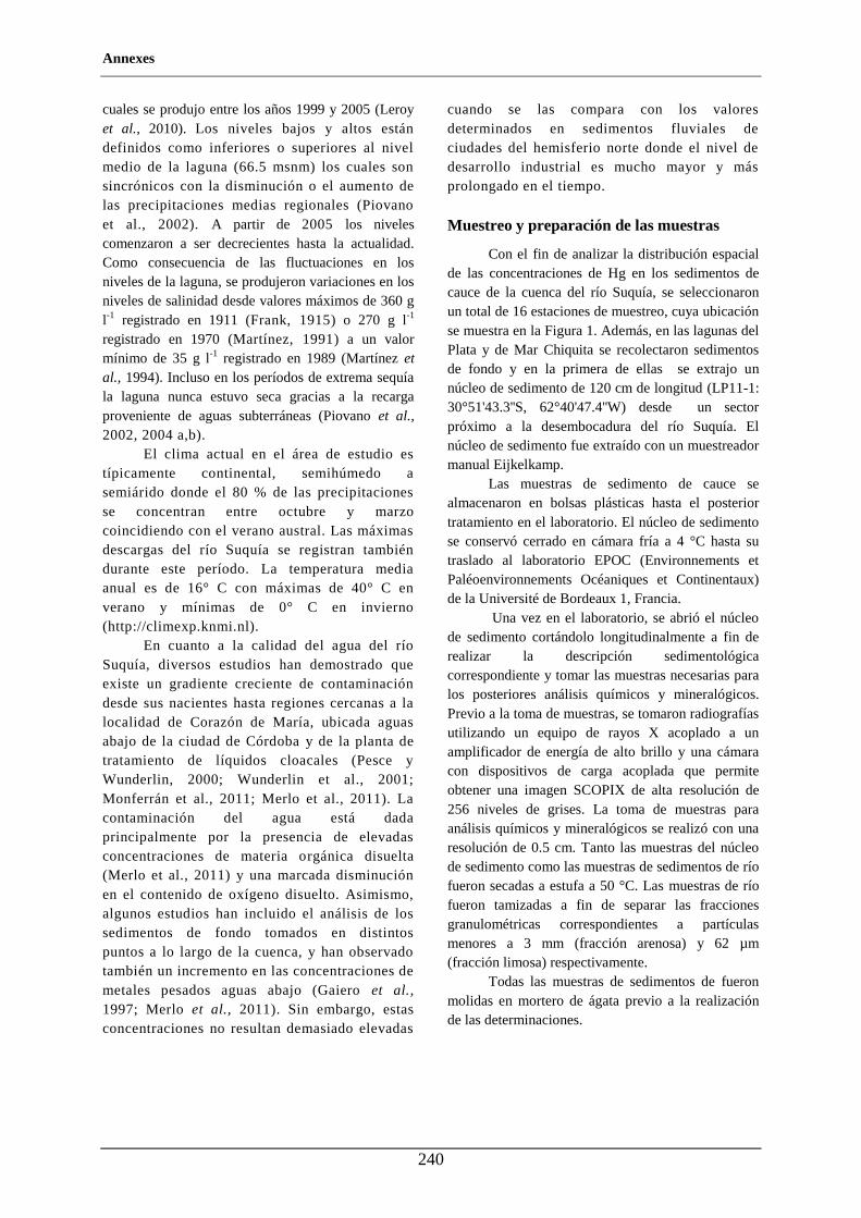
Annexes
240
cuales se produjo entre los años 1999 y 2005 (Leroy et al., 2010). Los niveles bajos y altos están definidos como inferiores o superiores al nivel medio de la laguna (66.5 msnm) los cuales son sincrónicos con la disminución o el aumento de las precipitaciones medias regionales (Piovano et al., 2002). A partir de 2005 los niveles comenzaron a ser decrecientes hasta la actualidad. Como consecuencia de las fluctuaciones en los niveles de la laguna, se produjeron variaciones en los niveles de salinidad desde valores máximos de 360 g l-1 registrado en 1911 (Frank, 1915) o 270 g l-1 registrado en 1970 (Martínez, 1991) a un valor mínimo de 35 g l-1 registrado en 1989 (Martínez et al., 1994). Incluso en los períodos de extrema sequía la laguna nunca estuvo seca gracias a la recarga proveniente de aguas subterráneas (Piovano et al., 2002, 2004 a,b).
El clima actual en el área de estudio es típicamente continental, semihúmedo a semiárido donde el 80 % de las precipitaciones se concentran entre octubre y marzo coincidiendo con el verano austral. Las máximas descargas del río Suquía se registran también durante este período. La temperatura media anual es de 16° C con máximas de 40° C en verano y mínimas de 0° C en invierno (http://climexp.knmi.nl).
En cuanto a la calidad del agua del río Suquía, diversos estudios han demostrado que existe un gradiente creciente de contaminación desde sus nacientes hasta regiones cercanas a la localidad de Corazón de María, ubicada aguas abajo de la ciudad de Córdoba y de la planta de tratamiento de líquidos cloacales (Pesce y Wunderlin, 2000; Wunderlin et al., 2001; Monferrán et al., 2011; Merlo et al., 2011). La contaminación del agua está dada principalmente por la presencia de elevadas concentraciones de materia orgánica disuelta (Merlo et al., 2011) y una marcada disminución en el contenido de oxígeno disuelto. Asimismo, algunos estudios han incluido el análisis de los sedimentos de fondo tomados en distintos puntos a lo largo de la cuenca, y han observado también un incremento en las concentraciones de metales pesados aguas abajo (Gaiero et al., 1997; Merlo et al., 2011). Sin embargo, estas concentraciones no resultan demasiado elevadas
cuando se las compara con los valores determinados en sedimentos fluviales de ciudades del hemisferio norte donde el nivel de desarrollo industrial es mucho mayor y más prolongado en el tiempo.
Muestreo y preparación de las muestras
Con el fin de analizar la distribución espacial de las concentraciones de Hg en los sedimentos de cauce de la cuenca del río Suquía, se seleccionaron un total de 16 estaciones de muestreo, cuya ubicación se muestra en la Figura 1. Además, en las lagunas del Plata y de Mar Chiquita se recolectaron sedimentos de fondo y en la primera de ellas se extrajo un núcleo de sedimento de 120 cm de longitud (LP11-1: 30°51'43.3''S, 62°40'47.4''W) desde un sector próximo a la desembocadura del río Suquía. El núcleo de sedimento fue extraído con un muestreador manual Eijkelkamp.
Las muestras de sedimento de cauce se almacenaron en bolsas plásticas hasta el posterior tratamiento en el laboratorio. El núcleo de sedimento se conservó cerrado en cámara fría a 4 °C hasta su traslado al laboratorio EPOC (Environnements et Paléoenvironnements Océaniques et Continentaux) de la Université de Bordeaux 1, Francia.
Una vez en el laboratorio, se abrió el núcleo de sedimento cortándolo longitudinalmente a fin de realizar la descripción sedimentológica correspondiente y tomar las muestras necesarias para los posteriores análisis químicos y mineralógicos. Previo a la toma de muestras, se tomaron radiografías utilizando un equipo de rayos X acoplado a un amplificador de energía de alto brillo y una cámara con dispositivos de carga acoplada que permite obtener una imagen SCOPIX de alta resolución de 256 niveles de grises. La toma de muestras para análisis químicos y mineralógicos se realizó con una resolución de 0.5 cm. Tanto las muestras del núcleo de sedimento como las muestras de sedimentos de río fueron secadas a estufa a 50 °C. Las muestras de río fueron tamizadas a fin de separar las fracciones granulométricas correspondientes a partículas menores a 3 mm (fracción arenosa) y 62 µm (fracción limosa) respectivamente.
Todas las muestras de sedimentos de fueron molidas en mortero de ágata previo a la realización de las determinaciones.
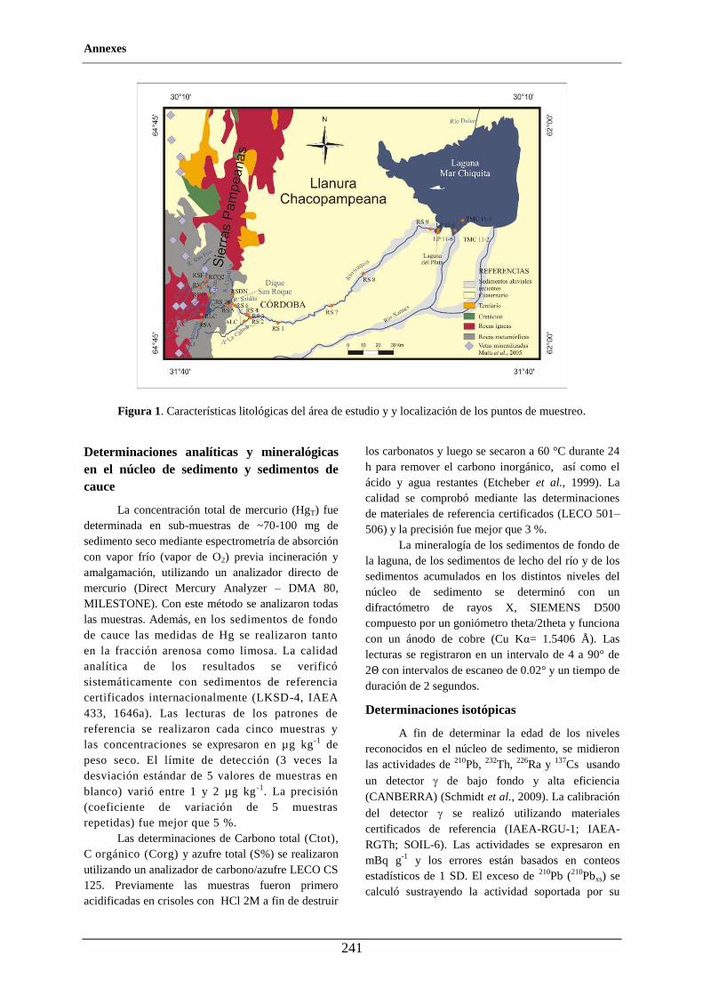
Annexes
241
Figura 1. Características litológicas del área de estudio y y localización de los puntos de muestreo.
Determinaciones analíticas y mineralógicas en el núcleo de sedimento y sedimentos de cauce
La concentración total de mercurio (HgT) fue determinada en sub-muestras de ~70-100 mg de sedimento seco mediante espectrometría de absorción con vapor frío (vapor de O2) previa incineración y amalgamación, utilizando un analizador directo de mercurio (Direct Mercury Analyzer – DMA 80, MILESTONE). Con este método se analizaron todas las muestras. Además, en los sedimentos de fondo de cauce las medidas de Hg se realizaron tanto en la fracción arenosa como limosa. La calidad analítica de los resultados se verificó sistemáticamente con sedimentos de referencia certificados internacionalmente (LKSD-4, IAEA 433, 1646a). Las lecturas de los patrones de referencia se realizaron cada cinco muestras y las concentraciones se expresaron en µg kg-1 de peso seco. El límite de detección (3 veces la desviación estándar de 5 valores de muestras en blanco) varió entre 1 y 2 µg kg-1. La precisión (coeficiente de variación de 5 muestras repetidas) fue mejor que 5 %.
Las determinaciones de Carbono total (Ctot), C orgánico (Corg) y azufre total (S%) se realizaron utilizando un analizador de carbono/azufre LECO CS 125. Previamente las muestras fueron primero acidificadas en crisoles con HCl 2M a fin de destruir
los carbonatos y luego se secaron a 60 °C durante 24 h para remover el carbono inorgánico, así como el ácido y agua restantes (Etcheber et al., 1999). La calidad se comprobó mediante las determinaciones de materiales de referencia certificados (LECO 501–506) y la precisión fue mejor que 3 %.
La mineralogía de los sedimentos de fondo de la laguna, de los sedimentos de lecho del río y de los sedimentos acumulados en los distintos niveles del núcleo de sedimento se determinó con un difractómetro de rayos X, SIEMENS D500 compuesto por un goniómetro theta/2theta y funciona con un ánodo de cobre (Cu Kα= 1.5406 Å). Las lecturas se registraron en un intervalo de 4 a 90° de 2Θ con intervalos de escaneo de 0.02° y un tiempo de duración de 2 segundos.
Determinaciones isotópicas
A fin de determinar la edad de los niveles reconocidos en el núcleo de sedimento, se midieron las actividades de 210Pb, 232Th, 226Ra y 137Cs usando
un detector de bajo fondo y alta eficiencia (CANBERRA) (Schmidt et al., 2009). La calibración
del detector se realizó utilizando materiales certificados de referencia (IAEA-RGU-1; IAEA-RGTh; SOIL-6). Las actividades se expresaron en mBq g-1 y los errores están basados en conteos estadísticos de 1 SD. El exceso de 210Pb (210Pbxs) se calculó sustrayendo la actividad soportada por su
Annexes
242
isótopo padre, 226Ra, de la actividad total del 210Pb en el sedimento. Los errores en 210Pbxs fueron calculados por propagación de los errores en el par correspondiente (210Pb y 226Ra).
Extracciones selectivas
Las extracciones selectivas se utilizan para determinar la asociación de elementos traza con diferentes fases mineralógicas u orgánicas presentes en suelos y sedimentos (e.g. Tessier et al., 1979, Audry et al., 2005). A fin de determinar las fases portadoras de Hg en el núcleo de sedimento estudiado, se realizaron extracciones selectivas de tres pasos, tal como se describe en Castelle et al. (2007). Los esquemas de extracciones paralelas similares al utilizado en este trabajo, evitan limitaciones tales como (i) la transferencia de metales de una fase a la otra (Bermond, 1992), (ii) múltiples riesgos de contaminación de muestras por los sucesivos reactivos usados (Quevauviller, 1998), (iii) posibles cambios en la especiación elemental durante las sucesivas extracciones y (iv) cambios o pérdidas de especies elementales durante el lavado del residuo (Rosenberg y Ariese, 2001). Además este método no muestra riesgos en la pérdida de muestras por lo que un error producido durante una de las extracciones no compromete a la secuencia entera (Tack et al., 1996).
Todas las soluciones utilizadas en los ensayos y determinaciones analíticas se prepararon a partir de reactivos de Grado Analítico y agua Milli-Q®. Todo el material de laboratorio en contacto con las muestras fue lavado previamente con HCl 10 % durante 3 días, enjuagado con agua Milli-Q® y secado bajo campana con flujo laminar.
En el extracto obtenido se realizaron determinaciones de las concentraciones de Hg siguiendo la metodología descrita anteriormente, así como de Fe y Mn que se midieron mediante espectrometría de absorción atómica por llama (Perkin Elmer AAnalyst 300). Los límites de detección (3 veces la desviación típica del blanco) fueron de 0.5 y 0.3 μg L-1 para Fe y Mn y la precisión fue mejor que 2 y 3%, respectivamente. El proceso de extracción selectiva comprendió las siguientes etapas:
Extracción con ascorbato (Hg asociado a la fracción reducible)
Este procedimiento permite extraer los elementos traza asociados con óxidos de Mn y la fracción más reactiva de los óxidos de Fe (i.e. óxidos amorfos; Kostka y Luther III, 1994; Audry et al.,
2006). La metodología consiste en suspender 200 mg de sedimento seco en 12.5 ml de solución 0.11M de ascorbato (5:5:2 citrato de sodio/bicarbonato de sodio/mezcla de ácido ascórbico; J.T. Baker). Se agita durante 24 h y luego se separa el residuo sólido mediante centrifugación durante 15 minutos a 9000 rpm. El residuo se enjuaga con agua Milli-Q®, se seca a 50° C y se muele en mortero de ágata hasta alcanzar fracciones de ~4µm. La fracción correspondiente al Hg reducible corresponde a la diferencia entre la concentración de Hg total (HgT) y el Hg determinado en el residuo.
Extracción con H2O2 (Hg asociado a la fracción oxidable)
El lavado de los sedimentos con H2O2 permite extraer los metales asociados con la materia orgánica y sulfuros minerales (Tessier et al., 1979). El método modificado por Ma y Uren (1995) y Audry et al. (2006), consiste en suspender 250 mg de sedimento seco en 8 ml de una solución de H2O2 al 30 % cuyo pH se fija en 5 mediante el agregado de NaOH. La suspensión resultante se calienta a 85° C durante 5 h. Al cabo de 3 h se agregan 3 ml de H2O2 30 % y 5 ml de acetato de amonio 5M mientras continúa calentándose. Después de 5 h, la suspensión se agita nuevamente durante 30 minutos y se centrifuga durante 15 minutos a 9000 rpm. El residuo sólido se lava con agua Milli-Q®, se seca y se muele en mortero de ágata. La fracción de Hg asociada a la materia orgánica y sulfuros se calcula restando a la concentración de HgT, la concentración de Hg determinada en el residuo resultante de esta extracción (Sahuquillo et al., 2003; Castelle et al., 2007).
Extracción con HCl (Hg asociado a la fracción soluble en ácido)
La fracción soluble en ácido fue diseñada empíricamente para extraer la mayor parte de los metales traza potencialmente biodisponibles (Bryan y Langston, 1992; Langston et al., 1999). Comprende metales adsorbidos o intercambiados, y aquellos que se encuentran co-precipitados en sales solubles y asociados a sulfuros volátiles ácidos (Huerta-Diaz y Morse 1990, 1992; Nova-López y Huerta-Díaz, 2001). La fracción correspondiente a los sulfuros volátiles ácidos se define operacionalmente como la fracción de sulfuros extraída mediante lavados con HCl 1M a temperatura ambiente. Esta fracción no incluye los óxidos de Fe cristalinos resultantes de la oxidación de monosulfuros (Raiswell et al., 1994).
Annexes
243
Para esta extracción se suspenden 200 mg de sedimento seco en 12.5 ml de HCl 1M y se agita durante 24 h. El residuo sólido se separa por centrifugación, se lava con agua Milli-Q®, se seca a 50° C y se muele en mortero de ágata. La concentración de Hg asociada a la fracción soluble se calcula como la diferencia entre la concentración de HgT y la concentración de Hg determinada en el residuo resultante de esta extracción (HgHCl; Castelle et al., 2007).
RESULTADOS
Descripción sedimentológica y geoquímica del núcleo de sedimento de la Laguna del Plata
La Figura 2 a y b muestra la fotografía y la imagen de RX obtenidas para el núcleo de sedimento de la Laguna del Plata (LP11-1) donde se observa una alternancia de laminaciones en tonos grises claros y oscuros que han permitido distinguir 5 unidades sedimentarias. La primera (A) se extiende desde el fondo del núcleo de sedimento (120 cm) hasta los 75 cm y se trata de una secuencia masiva (sin laminaciones) que está separada de la inmediata superior mediante un contacto neto. Entre los 75 y 69 cm se observa una pequeña secuencia (B) que muestra una laminación producida por la alternancia de sedimentos oscuros y claros. Por encima de esta secuencia y hasta los 53 cm se distingue una nueva secuencia (C) caracterizada por la alternancia de capas de sedimento predominantemente claras. Entre los 53 y 16 cm de profundidad, se distingue una nueva secuencia (D) formada por la alternancia de laminaciones oscuras y claras, pero con contactos más netos que en los casos anteriores. Finalmente, en los 16 cm superiores se observa la secuencia superior (E) caracterizada por la acumulación de sedimentos de color verde oliva oscuro.
Las características sediment-ológicas del núcleo de sedimento fueron además contrastadas con algunas de las propiedades físicas y químicas determinadas en él (Figura 2 c-e). De acuerdo con lo observado en estas figuras, los mayores valores de porosidad (75 %) se determinaron cerca de la superficie del núcleo de sedimento mientras que los más bajos (~40 %) fueron registrados en la porción inferior (Figura 2 c). La laminación descrita anteriormente pareciera estar relacionada con
estos cambios de porosidad: la sección A muestra los menores valores, las secciones B, C y D valores intermedios, mientras que la secuencia E muestra los valores más altos (Figura 2 c).
La variación del contenido de Corg a lo largo del núcleo de sedimento se muestra en la Figura 2d. Las concentraciones varían entre ~0.5 y ~2.8 %, encontrándose los máximos valores en los primeros 15 cm y entre los 40 y 60 cm de profundidad. En el resto del núcleo de sedimento, los valores permanecen más o menos constantes entre 0.6 y ~0.9 %. Probablemente como consecuencia de las escasas precipitaciones y la elevada salinidad del agua, los niveles de Corg medidos en el núcleo de sedimento de la Laguna del Plata son marcadamente inferiores a los medidos en lagos de la Patagonia andina, donde se han reportado valores de entre 6 y 8 % Corg en lagos del Norte (i.e. Ribeiro Guevara et al., 2010) y entre 12 y 15 % de Corg en lagos más australes (Hermanns y Biester, 2013). Los valores de Corg son importantes indicadores de aportes de Hg a partir de la erosión de suelos en las cabeceras de los lagos debido a la fuerte afinidad de este elemento por la materia orgánica (Driscoll et al., 1995; Rydberg et al., 2010; Teisserenc et al., 2010).
Las concentraciones de S a lo largo del
núcleo de sedimento oscilan entre 3 y 11 %. El perfil de concentraciones (Figura 2 e) muestra tres zonas donde se registran los máximos valores: por debajo de los 100 cm de profundidad, entre los 75 y 35 cm y por encima de los 16 cm de profundidad. Estas concentraciones corresponderían principalmente a sulfuros diseminados en los sedimentos dado que no se ha determinado la presencia de yeso a lo largo del núcleo de sedimento.
Las concentraciones de Fe y Mn fueron medidas en los sobrenadantes de la extracción con ascorbato (Fe y Mn-asc). Desde la parte más profunda del núcleo de sedimento (120 cm) hasta los 74 cm el valor promedio de Fe es de 1670 mg kg-1, en la parte central hasta los 16 cm es de 1270 mg kg-1 y en la parte más superficial es de 2240 mg kg-1. En los mismos intervalos, las concentraciones de Mn promedian 1410, 1790 y 1510 mg kg-1respectivamente.
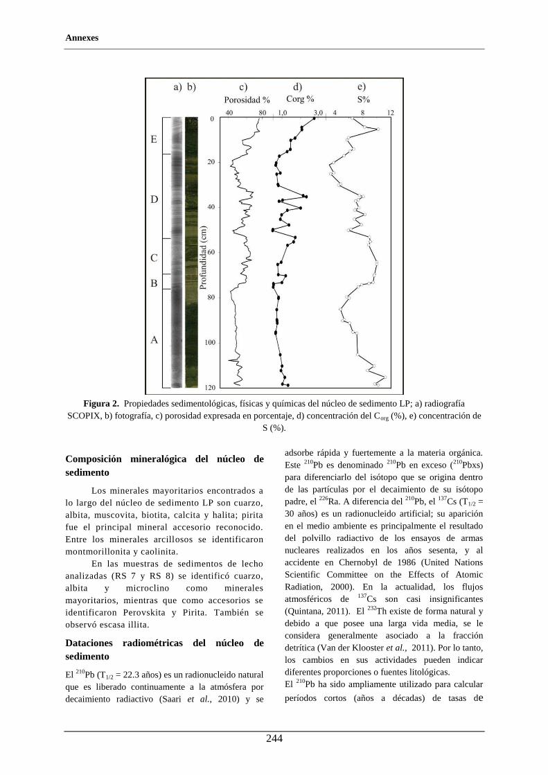
Annexes
244
Figura 2. Propiedades sedimentológicas, físicas y químicas del núcleo de sedimento LP; a) radiografía
SCOPIX, b) fotografía, c) porosidad expresada en porcentaje, d) concentración del Corg (%), e) concentración de S (%).
Composición mineralógica del núcleo de sedimento
Los minerales mayoritarios encontrados a lo largo del núcleo de sedimento LP son cuarzo, albita, muscovita, biotita, calcita y halita; pirita fue el principal mineral accesorio reconocido. Entre los minerales arcillosos se identificaron montmorillonita y caolinita.
En las muestras de sedimentos de lecho analizadas (RS 7 y RS 8) se identificó cuarzo, albita y microclino como minerales mayoritarios, mientras que como accesorios se identificaron Perovskita y Pirita. También se observó escasa illita.
Dataciones radiométricas del núcleo de sedimento
El 210Pb (T1/2 = 22.3 años) es un radionucleido natural que es liberado continuamente a la atmósfera por decaimiento radiactivo (Saari et al., 2010) y se
adsorbe rápida y fuertemente a la materia orgánica. Este 210Pb es denominado 210Pb en exceso (210Pbxs) para diferenciarlo del isótopo que se origina dentro de las partículas por el decaimiento de su isótopo padre, el 226Ra. A diferencia del 210Pb, el 137Cs (T1/2 = 30 años) es un radionucleido artificial; su aparición en el medio ambiente es principalmente el resultado del polvillo radiactivo de los ensayos de armas nucleares realizados en los años sesenta, y al accidente en Chernobyl de 1986 (United Nations Scientific Committee on the Effects of Atomic Radiation, 2000). En la actualidad, los flujos atmosféricos de 137Cs son casi insignificantes (Quintana, 2011). El 232Th existe de forma natural y debido a que posee una larga vida media, se le considera generalmente asociado a la fracción detrítica (Van der Klooster et al., 2011). Por lo tanto, los cambios en sus actividades pueden indicar diferentes proporciones o fuentes litológicas. El 210Pb ha sido ampliamente utilizado para calcular
períodos cortos (años a décadas) de tasas de
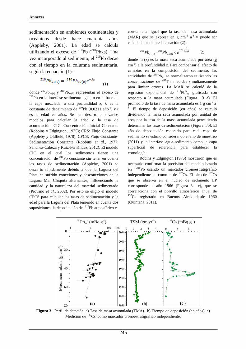
Annexes
245
sedimentación en ambientes continentales y oceánicos desde hace cuarenta años (Appleby, 2001). La edad se calcula utilizando el exceso de 210Pb (210Pbxs). Una vez incorporado al sedimento, el 210Pb decae con el tiempo en la columna sedimentaria, según la ecuación (1):
(1)
donde 210Pbxs(z) y 210Pbxs(0) representan el exceso de 210Pb en la interfase sedimento-agua, o en la base de
la capa mezclada, a una profundidad z, es la constante de decaimiento de 210Pb (0.0311 año-1) y t es la edad en años. Se han desarrollado varios modelos para calcular la edad o la tasa de acumulación: CIC: Concentración Inicial Constante (Robbins y Edgington, 1975); CRS: Flujo Constante (Appleby y Oldfield, 1978); CFCS: Flujo Constante-Sedimentación Constante (Robbins et al., 1977; Sanchez-Cabeza y Ruiz-Fernández, 2012). El modelo CIC en el cual los sedimentos tienen una concentración de 210Pb constante sin tener en cuenta las tasas de sedimentación (Appleby, 2001) se descartó rápidamente debido a que la Laguna del Plata ha sufrido conexiones y desconexiones de la Laguna Mar Chiquita alternantes, influenciando la cantidad y la naturaleza del material sedimentado (Piovano et al., 2002). Por esto se eligió el modelo CFCS para calcular las tasas de sedimentación y la edad para la Laguna del Plata teniendo en cuenta dos suposiciones: la depositación de 210Pb atmosférico es
constante al igual que la tasa de masa acumulada (MAR) que se expresa en g cm-2 a-1 y puede ser calculada mediante la ecuación (2) :
MARm
xszxs
z
ePbPb )0(
210)(
210 (2)
donde m (z) es la masa seca acumulada por área (g cm-2) a la profundidad z. Para compensar el efecto de cambios en la composición del sedimento, las actividades de 210Pbxs se normalizaron utilizando las concentraciones de 232Th, medidas simultáneamente para limitar errores. La MAR se calculó de la regresión exponencial de 210Pbn
xs graficada con respecto a la masa acumulada (Figura 3 a). El promedio de la tasa de masa acumulada es 1 g cm-2 a-
1. El tiempo de deposición (en años) se calculó dividiendo la masa seca acumulada por unidad de área por la tasa de la masa acumulada permitiendo determinar las tasas de sedimentación (Figura 3b). El año de depositación esperado para cada capa de sedimento se estimó considerando el año de muestreo (2011) y la interfase agua-sedimento como la capa superficial de referencia para establecer la cronología.
Robins y Edgington (1975) mostraron que es necesario confirmar la precisión del modelo basado en 210Pb usando un marcador cronoestratigráfico independiente tal como el de 137Cs. El pico de 137Cs que se observa en el núcleo de sedimento LP corresponde al año 1966 (Figura 3 c), que se correlaciona con el polvillo atmosférico anual de 137Cs registrado en Buenos Aires desde 1960 (Quintana, 2011).
Figura 3. Perfil de datación. a) Tasa de masa acumulada (TMA). b) Tiempo de deposición (en años). c)
Medición de 137Cs como marcador cronoestratigráfico independiente.
Annexes
246
Concentraciones de Hg total e identificación de fases portadoras en el núcleo de sedimento
HgT y tasas de acumulación
Las concentraciones de HgT medidas en intervalos de 0.5 cm a lo largo del núcleo de sedimento de la Laguna del Plata, varían entre ~13 y
~131 µg kg-1 (Figura 4 a). Las concentraciones más bajas y constantes se midieron desde la base del núcleo de sedimento y hasta los 75 cm de profundidad alcanzando un valor promedio de ~17.4 ± 1.6 µg kg-1. Por encima de los 75 cm, las concentraciones de HgT son muy variables. Por ejemplo, entre los 75 y 45 cm de profundidad, la concentración promedio determinada es de 39.8 ± 15.6 µg kg-1. Por encima de los 45 cm y hasta los 16 cm, se encuentran las concentraciones promedio de HgT más elevadas de 79.9 ± 27.5 µg kg-1 con picos de 89.7, 131.5 y 87.3 µg kg-1 observados a los 43.2, 36.7 y 30.2 cm respectivamente. En los primeros 16 cm de profundidad, la concentración promedio de HgT es menor, alcanzando un valor de 54.7 ± 16.1 µg kg-1. Estos valores se encuentran dentro del intervalo informado en lagos de la Patagonia y de otras regiones remotas de mundo que no están directamente afectadas por la actividad del hombre (Ribeiro Guevara et al., 2010; Hermanns y Biester, 2013; Conaway et al., 2012; Yang et al., 2010). Por ejemplo en la Patagonia argentina las concentraciones de Hg varían entre 50 y 200 µg kg-1 (Ribeiro Guevara et al., 2010) mientras que en la Patagonia chilena lo hacen entre 28 y 73 µg kg-1 (Hermanns y Biester, 2013) y en el lago Tanganyika (África) entre 20 y 90 µg kg-1 (Conaway et al., 2012). Concentraciones de Hg mayores se midieron en regiones más industrializadas o afectadas por actividades mineras. Por ejemplo, Castelle et al. (2007) informan concentraciones entre 490 y 5460 µg kg-1 en una zona minera francesa, mientras que Xia et al. (2001) informan una concentración promedio de Hg de 90 µg kg-1 en una reserva natural de humedales en el sur de China afectada por la contaminación derivada de la quema de combustibles fósiles. De acuerdo con las dataciones radiométricas los sedimentos acumulados en el segmento comprendido entre los 16 y los 75 cm se depositaron entre los años 1968 y 2003, período que además coincide con un máximo hidrológico (Figura 4 b) determinado para el sistema de lagunas del Plata/Mar Chiquita (Piovano et al., 2002, 2004 a,b). Los sedimentos más modernos presentan también concentraciones elevadas, aunque en promedio
inferiores a las registradas en el período 1968-2003, con una tendencia creciente hacia la parte más alta del núcleo de sedimento. La masa acumulada de sedimento por unidad de área se calculó en base a los datos de la densidad efectiva cada 0.5 cm de profundidad. Con este valor se calculó la masa acumulada de Hg por cm2 a lo largo del registro sedimentario de la laguna (Figura 4 c). Los valores determinados en la parte más baja del núcleo de sedimento (de 120 a 75 cm) son muy constantes y alcanzan un valor promedio de
0.02 ± 0.003 g cm-2 a-1. Por encima de los 75 cm y hasta los 45 cm, la masa acumulada de Hg se incrementa notablemente alcanzando un valor
promedio de 0.038 ± 0.016 g cm-2 a-1, lo cual supone un incremento promedio de 1.7 veces, en relación con la tasa determinada en el segmento inmediatamente inferior. Este aumento se intensifica aún más en los sedimentos depositados entre los 45 y 16 cm de profundidad, donde la masa acumulada de
Hg alcanza un valor promedio de 0.078 ± 0.022 g
cm-2 a-1, con un pico de 0.135 g cm-2 a-1 Hg a los 35 cm de profundidad. Los sedimentos más modernos, acumulados por encima de los 16 cm de profundidad, muestran una masa acumulada de Hg que en
promedio es 2 veces inferior (0.041 ± 0.014 g cm-2
a-1 Hg) que el período anterior pero al mismo tiempo
resulta 2 veces superior al valor promedio medido en la base del núcleo de sedimento. El aumento gradual de los flujos de Hg hacia la parte superior de los núcleos de sedimento extraídos en lagos de regiones remotas de la Tierra ha sido asignado al aumento del Hg atmóférico global. Para diferenciar estos aportes, se tomó como valor de referencia de condiciones no afectadas por los aportes atmosféricos a las concentraciones promedio de Hg medidas en la base del núcleo de sedimento (sedimentos acumulados antes de 1968). Este supuesto se basa en la constancia de los valores registrados en ese tramo del registro sedimentario y en la similitud de los mismos con las concentraciones de Hg medidas en los sedimentos de la cuenca del río Suquía (Tabla 1), lo cual sugiere que estos sedimentos podrían haber sido la principal fuente de aporte de Hg a la laguna en los años previos a 1968. La Figura 4 d muestra la variación de la relación entre los valores de la masa acumulada de Hg a lo largo del núcleo de sedimento y el correspondiente valor de fondo. En ella se observa el incremento gradual en la tasa de acumulación de Hg a partir del año 1968, alcanzado
valores que son 3.5 veces superiores en los sedimentos acumulados en el año 2011, en relación
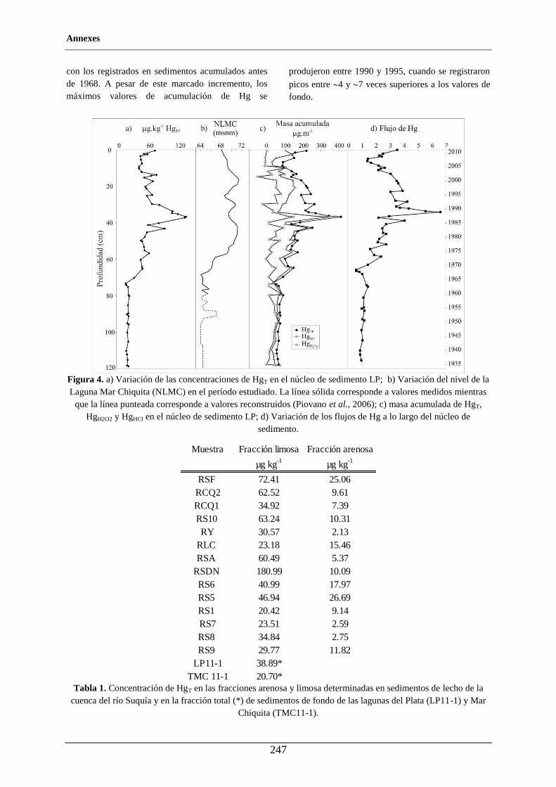
Annexes
247
con los registrados en sedimentos acumulados antes de 1968. A pesar de este marcado incremento, los máximos valores de acumulación de Hg se
produjeron entre 1990 y 1995, cuando se registraron
picos entre 4 y 7 veces superiores a los valores de fondo.
Figura 4. a) Variación de las concentraciones de HgT en el núcleo de sedimento LP; b) Variación del nivel de la Laguna Mar Chiquita (NLMC) en el período estudiado. La línea sólida corresponde a valores medidos mientras
que la línea punteada corresponde a valores reconstruidos (Piovano et al., 2006); c) masa acumulada de HgT, HgH2O2 y HgHCl en el núcleo de sedimento LP; d) Variación de los flujos de Hg a lo largo del núcleo de
sedimento.
Tabla 1. Concentración de HgT en las fracciones arenosa y limosa determinadas en sedimentos de lecho de la
cuenca del río Suquía y en la fracción total (*) de sedimentos de fondo de las lagunas del Plata (LP11-1) y Mar Chiquita (TMC11-1).
Muestra Fracción limosa Fracción arenosa
µg kg-1 µg kg-1
RSF 72.41 25.06RCQ2 62.52 9.61RCQ1 34.92 7.39RS10 63.24 10.31RY 30.57 2.13
RLC 23.18 15.46RSA 60.49 5.37
RSDN 180.99 10.09RS6 40.99 17.97RS5 46.94 26.69RS1 20.42 9.14RS7 23.51 2.59RS8 34.84 2.75RS9 29.77 11.82
LP11-1 38.89*TMC 11-1 20.70*
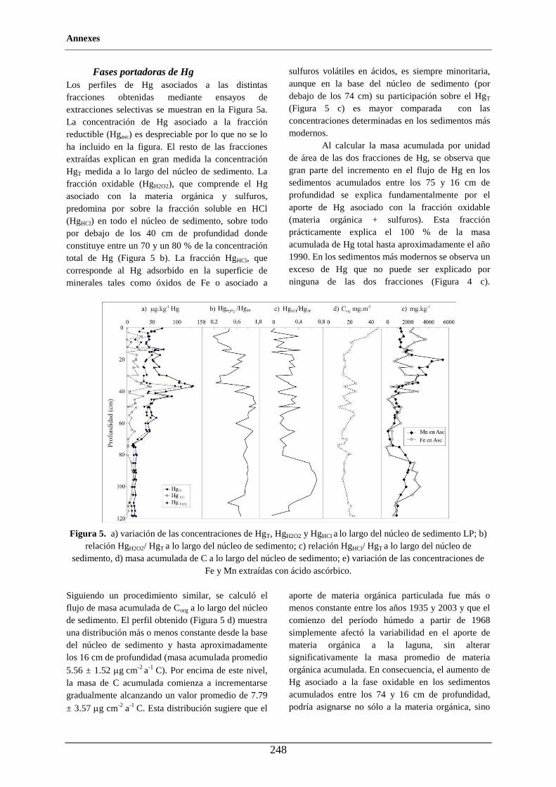
Annexes
248
Fases portadoras de Hg Los perfiles de Hg asociados a las distintas fracciones obtenidas mediante ensayos de extracciones selectivas se muestran en la Figura 5a. La concentración de Hg asociado a la fracción reductible (Hgasc) es despreciable por lo que no se lo ha incluido en la figura. El resto de las fracciones extraídas explican en gran medida la concentración HgT medida a lo largo del núcleo de sedimento. La fracción oxidable (HgH2O2), que comprende el Hg asociado con la materia orgánica y sulfuros, predomina por sobre la fracción soluble en HCl (HgHCl) en todo el núcleo de sedimento, sobre todo por debajo de los 40 cm de profundidad donde constituye entre un 70 y un 80 % de la concentración total de Hg (Figura 5 b). La fracción HgHCl, que corresponde al Hg adsorbido en la superficie de minerales tales como óxidos de Fe o asociado a
sulfuros volátiles en ácidos, es siempre minoritaria, aunque en la base del núcleo de sedimento (por debajo de los 74 cm) su participación sobre el HgT (Figura 5 c) es mayor comparada con las concentraciones determinadas en los sedimentos más modernos. Al calcular la masa acumulada por unidad de área de las dos fracciones de Hg, se observa que gran parte del incremento en el flujo de Hg en los sedimentos acumulados entre los 75 y 16 cm de profundidad se explica fundamentalmente por el aporte de Hg asociado con la fracción oxidable (materia orgánica + sulfuros). Esta fracción prácticamente explica el 100 % de la masa acumulada de Hg total hasta aproximadamente el año 1990. En los sedimentos más modernos se observa un exceso de Hg que no puede ser explicado por ninguna de las dos fracciones (Figura 4 c).
Figura 5. a) variación de las concentraciones de HgT, HgH2O2 y HgHCl a lo largo del núcleo de sedimento LP; b)
relación HgH2O2/ HgT a lo largo del núcleo de sedimento; c) relación HgHCl/ HgT a lo largo del núcleo de sedimento, d) masa acumulada de C a lo largo del núcleo de sedimento; e) variación de las concentraciones de
Fe y Mn extraídas con ácido ascórbico. Siguiendo un procedimiento similar, se calculó el flujo de masa acumulada de Corg a lo largo del núcleo de sedimento. El perfil obtenido (Figura 5 d) muestra una distribución más o menos constante desde la base del núcleo de sedimento y hasta aproximadamente los 16 cm de profundidad (masa acumulada promedio
5.56 ± 1.52 g cm-2 a-1 C). Por encima de este nivel, la masa de C acumulada comienza a incrementarse gradualmente alcanzando un valor promedio de 7.79
± 3.57 g cm-2 a-1 C. Esta distribución sugiere que el
aporte de materia orgánica particulada fue más o menos constante entre los años 1935 y 2003 y que el comienzo del período húmedo a partir de 1968 simplemente afectó la variabilidad en el aporte de materia orgánica a la laguna, sin alterar significativamente la masa promedio de materia orgánica acumulada. En consecuencia, el aumento de Hg asociado a la fase oxidable en los sedimentos acumulados entre los 74 y 16 cm de profundidad, podría asignarse no sólo a la materia orgánica, sino
Annexes
249
también a la presencia de otras fases oxidables en el sedimento, muy probablemente pirita dado que este mineral ha sido identificado mediante los análisis de difracción de rayos X. La distribución de las concentraciones de Fe y Mn medidas en los extractos realizados con ácido ascórbico indica una fuerte presencia de los correspondientes óxidos por debajo de los 80 cm de profundidad y por encima de los 40 cm en el núcleo de sedimento estudiado (Figura 5 e). Dado que las concentraciones de Hg determinadas en esos mismos extractos son despreciables, es posible inferir que el Hg presente en los sedimentos acumulados en esos niveles no estaría asociado con patinas de óxidos de Fe y Mn. DISCUSIÓN
Los perfiles de concentración del HgT y de las fracciones de Hg asociado con fases oxidables y con fases biodisponibles indican que a partir del año 1968 se inicia un período de gradual aumento de las concentraciones en relación con lo observado en los sedimentos acumulados previamente y que perdura hasta la actualidad. Este comportamiento coincide con un importante incremento en el nivel de la laguna de Mar Chiquita (Figura 4b) que comenzó a partir del año 1968 y que culminó en el año 2003 cuando se inició un período de bajante. Además del fuerte incremento en las concentraciones de Hg, se observó un aumento en la variabilidad de las mismas, que podría estar relacionado con las fluctuaciones de nivel registradas durante ese período. Debido a que no existen registros de nivel en la laguna del Plata, los valores que aquí se utilizan corresponden a los medidos en la laguna de Mar Chiquita, la cual se mantuvo conectada con la laguna del Plata durante todo el período húmedo. Los sedimentos acumulados en la laguna antes de 1968 presentan concentraciones bajas de Hg y relativamente constantes. La reconstrucción paleoclimática de la región indica que en este período predominaron condiciones de mayor aridez que dieron lugar a una fuerte contracción de la superficie de la laguna. En consecuencia, durante ese período la principal fuente de aporte de sedimentos a la laguna habría correspondido a los sedimentos transportados por el río Suquía desde las cabeceras de la cuenca y al aporte desde las precipitaciones, fundamentalmente en forma de polvo atmosférico. Considerando que la naturaleza de los sedimentos de lecho se ha mantenido invariable con el tiempo (sobre todo de aquellos que se encuentran en las
cabeceras de la cuenca donde no hay una fuerte intervención del hombre) sería válido pensar que las concentraciones de Hg medidas en sedimentos actuales de lecho representan el aporte de este elemento a la laguna a lo largo del tiempo. Las concentraciones más altas de Hg medidas en los sedimentos tomados en las cabeceras de la cuenca (Tabla 1) sugiere que la fuente de este elemento estaría relacionada con la presencia de sedimentos volcaniclásticos predominantes en el sector NO así como también de sulfuros diseminados o en vetas (Mutti et al., 2005). Además, el aporte proveniente de actividades industriales desarrolladas en el tramo medio de la cuenca pareciera ser despreciable dado que los niveles de Hg se mantienen más o menos constantes desde la ciudad de Córdoba hasta la desembocadura del río en la Laguna del Plata. Durante el período seco únicamente los sedimentos más finos pudieron alcanzar la laguna, lo cual refuerza la hipótesis del aporte desde los sedimentos de la cuenca, debido a que el Hg se concentra fundamentalmente en la fracción más fina de los mismos (Tabla 1). La especiación sólida del Hg en el segmento más profundo del núcleo de sedimento indica que este elemento se encuentra principalmente asociado con la fracción oxidable de los sedimentos. En esta parte del núcleo de sedimento además, la concentración de Corg es la menor (Figura 2e) y la de S total es la mayor (Figura 2) lo cual sugiere fuertemente que el Hg acumulado en la laguna del Plata antes de 1968 se encuentra asociado a sulfuros de metal probablemente aportados desde la fracción más fina de los sedimentos provenientes de las cabeceras de la cuenca. El HgS(s) es relativamente insoluble y menos volátil que otras formas de Hg (Barnett y Turner, 2001), lo cual lo convierte en una fase estable en los sedimentos. Sin embargo, la presencia de este mineral no ha sido descrita en la región, por lo que se estima que se encuentra asociado preferentemente con la pirita. Este último, además de ser un mineral muy común en los ambientes sedimentarios y de haber sido identificado tanto en los sedimentos acumulados en la laguna como en los sedimentos de lecho del río Suquía, es capaz de adsorber muchos elementos potencialmente tóxicos como Hg, Pb, Cu, Cd, Cr y As (por ejemplo, Bostick et al., 2003; Doyle et al., 2004; Borah y Senapati, 2006; Ozverdi y Erdem, 2006). El Hg se adsorbe en la superficie de la pirita en un amplio intervalo de pH (Behra et al., 2001) formando principalmente complejos de Hg-Cl y Hg-OH (por ejemplo, Behra et al., 2001; Bower et al., 2008). En la laguna del Plata, la formación de
Annexes
250
estos complejos estaría favorecida además por la elevada salinidad y el pH alcalino del agua (~42 g L-1
y pH ~9.2). En los sedimentos acumulados después de 1968 las concentraciones de HgT aumentan en relación con los niveles más antiguos. Esta situación coincide con el inicio de un período más húmedo en la región que se tradujo en un aumento en los niveles de las lagunas estudiadas. Al igual que en la parte más baja del núcleo de sedimento, el Hg se encuentra principalmente asociado con la fracción oxidable, pero en este tramo en particular, la concentración de Corg es ligeramente mayor, lo cual sugiere que el Hg estaría principalmente asociado con la materia orgánica y en menor medida se encontraría adsorbido tanto en sulfuros (en períodos de mayor humedad y de condiciones reductoras predominantes), como en arcillas y pátinas de (hidr)óxidos de Fe y Mn (en períodos más secos y oxidantes). En el perfil de HgT (Figura 4a) se observa un pico
(131 g kg-1) asociado a sedimentos acumulados aproximadamente entre los años 1990-1995. Este pico coincide además con un con un pico en las concentraciones de HgH2O2 (Figura 5 b) y elevado porcentaje de Corg (Figura 5 d) lo cual sugiere que la laguna estuvo afectada por algún factor o evento que dio lugar a una acumulación de Hg superior a la registrada en períodos anteriores y posteriores y que además promovió la actividad biológica en la laguna. Entre las diferentes fuentes de Hg descritas en sistemas naturales, se menciona el aporte desde emisiones volcánicas (i.e., Fitzgerald y Lamborg, 2003, Selin, 2009). Debido a la proximidad del sistema volcánico andino y a su conocida influencia sobre el área de estudio (i.e., Gaiero et al., 2007; Osores et al., 2011), es posible pensar que los niveles más importantes registrados en el núcleo de sedimento puedan ser consecuencia de aportes desde erupciones volcánicas producidas en los últimos ~80 años. Además, es conocido el efecto de fertilización que tienen los elementos asociados con las cenizas, tales como P, Fe y otros elementos traza, sobre los ecosistemas acuáticos (Hamme et al., 2010; Lin et al., 2011). En ambientes marinos, por ejemplo, se ha demostrado que luego de una erupción volcánica se produce un incremento en la concentración de clorofila, la cual es tomada como un proxy de biomasa planctónica (Hamme et al., 2010; Lin et al., 2011). En consecuencia, un potencial aporte de Hg desde tefras provenientes de una erupción volcánica podría haber generado, no sólo un aporte extraordinario de Hg a la laguna del Plata, sino
también podría haber dado lugar a un proceso de fertilización que se ve reflejado en el registro sedimentario como un aumento en el contenido de Corg. El registro de erupciones volcánicas más próximas al área de estudio, indica que la más cercana al momento en que se registró el pico fue la erupción del volcán Láscar (5592 m; 23.22ºS, 67.44ºW), ubicado en el Norte de Chile sobre el límite con Argentina. Desde 1984 hasta 1993, la actividad del volcán Láscar fue intensa y estuvo caracterizada por ciclos de crecimiento y subsidencia de domos dacíticos de lava, desgasificación del magma representada por una actividad fumarólica intensa y eventos eruptivos vulcanianos a plinianos. La erupción del 19 y 20 de Abril de 1993 fue la más intensa del registro histórico del volcán Láscar y durante la misma se formó un extenso penacho de dirección E-SE que alcanzó la costa atlántica sudamericana (Matthews et al., 1997) y muy probablemente la laguna del Plata. Por encima del mencionado pico de Hg, la masa acumulada de HgT por unidad de área comienza a disminuir gradualmente, y conserva esta tendencia
hasta los 7 cm de profundidad, cuando comienza a aumentar nuevamente. Es interesante notar que la masa acumulada de HgT no puede ser completamente explicada por las fracciones oxidable y biodisponibles en ese tramo del núcleo de sedimento, lo cual permite suponer un aporte que podría estar asociado al Hg atmosférico.
CONCLUSIONES
Los niveles de Hg medidos en sedimentos actuales y pasados acumulados en la cuenca del río Suquía (en promedio: 47±30 µg kg-1) son bajos en relación con niveles medidos en otras regiones del mundo altamente industrializadas o afectadas por actividades mineras, pero están dentro del intervalo de valores determinados en lagos ubicados en regiones remotas de la Patagonia andina. Las importantes variaciones en los niveles de Hg observadas en el núcleo de sedimento extraído de la laguna del Plata parecieran responder a los cambios hidrológicos registrados en el sistema en los últimos ~80 años, más que a eventos de contaminación puntuales. Durante el período seco que afectó la región de la laguna antes de 1968, la principal fuente de aporte de sedimentos a la laguna habría correspondido a los sedimentos transportados por el río Suquía desde las cabeceras de la cuenca y al aporte desde las precipitaciones, fundamentalmente en forma de
Annexes
251
polvo atmosférico. La inexistencia de otras fuentes de Hg que afecten la región, así como también de mecanismos que alteren la especiación y distribución del Hg entre las fases sólida y acuosa, explica la constancia en las concentraciones de Hg registradas en la base del núcleo de sedimento y también son similares a las medidas en los sedimentos de la cuenca del río Suquía. En este tramo, el Hg se encuentra principalmente asociado con la fracción oxidable de los sedimentos, atribuible en mayor medida a la pirita (sobre la que el Hg se encontraría adsorbido) y en menor medida a la presencia de materia orgánica particulada. En los sedimentos acumulados después de 1968 el aumento en las concentraciones de HgT coincide con el inicio de un período más húmedo en la región, al menos hasta el año 2003. En ese período el Hg geogénico habría llegado a la laguna adsorbido en pirita y en menor medida asociado a óxidos de Fe y Mn presentes en los sedimentos de lecho. Una vez en la laguna se habría producido una posterior removilización y transporte partir de procesos biogeoquímicos. El pico de concentración de Hg registrado en sedimentos acumulados entre 1990 y 1995 se atribuye al aporte desde las cenizas volcánicas que alcanzaron la región luego de la erupción del volcán Lascar en 1993. Estas cenizas no sólo aportaron Hg a los sedimentos sino que además desencadenaron un aumento en la actividad biológica de la laguna que se tradujo en la presencia de mayores concentraciones de Corg en los sedimentos de ese período y una mayor asociación del Hg con esa fase. El continuo crecimiento de las concentraciones de Hg en los sedimentos más modernos (acumulados desde 2003), asociado con un ciclo de bajas precipitaciones en la región, se atribuye a la influencia del Hg antropogénico, incorporado desde la atmósfera y cuyo efecto ha sido descrito en otras regiones del extremo sur de América del Sur menos afectadas por la actividad del hombre. Agradecimientos. Los autores desean agradecer la asistencia del Consejo Nacional de Investigaciones Científicas y Técnicas (CONICET), de la Universidad Nacional de Córdoba y de la Université de Bordeaux 1. Este trabajo fue parcialmente financiado con fondos otorgados por SECYT-UNC y PIP-CONICET. Yohana V. Stupar agradece una beca Erasmus Mundus otorgada por la Unión Europea. Asimismo, los autores agradecen las sugerencias de Anne M. Hansen y otros dos revisores anónimos que
contribuyeron a mejorar significativamente el presente trabajo. REFERENCIAS
Appleby, P.G., Oldfield, F., 1978, The calculation of lead-210 dates assuming a constant rate of supply of unsupported 210Pb to the sediment: Catena, 5 (1), 1-8.
Appleby, P.G., 2001, Chronostratigraphic techniques in recent sediments, in Last, W.M. and Smol, J.P. (eds.), Tracking Environmental Change Using Lake Sediments, Volume 1: Basin Analysis, Coring and Chronological Techniques: Dordrecht, The Netherlands Kluwer Academic Publishers, 171-203.
Audry, S., Blanc, G., Schäfer, J., 2006, Solid state partitioning of trace metals in suspended particulate matter from a river system affected by smelting waste drainage: Science of the Total Environment, 363, 216-236.
Audry, S., Blanc, G., Schäfer. J., 2005, The impact of sulphide oxidation on dissolved metal (Cd, Zn, Cu, Cr, Co, Ni, U) inputs into the Lot-Garonne fluvial system (France): Applied Geochemistry 20 (5), 919-931.
Balcom, P., Fitzgerald W., Hammerschmidt, C., Lamborg, C., Graham, L., 2004, Mercury sources and speciation in the waters of New York/New Jersey Harbor Estuary: Materials and Geoenvironment, 51, 795-798.
Barnett, M.O., Turner, R.R., 2001, Bioaccessibility of mercury in soils: Soil and Sediment Contamination, 10, 301-316.
Behra, P., Bonnissel-Gissinger, P., Alnot, M., Revel, R., Ehrhardt, J.J., 2001, XPS and XAS study of the sorption of Hg(II) onto pyrite: Langmuir, 17, 3970-3979,
Bermond, A.P., 1992, Thermodynamics applied to the study of the limits of sequential extraction procedures used for the speciation of trace elements in sediments and soils: Environmental Technology, 13 (12), 1175-1179. Biester, H., Bindler, R., Martínez-Cortizas, A., Engstrom, D., 2007, Modeling the past atmospheric deposition of mercury using natural archives: Environmental Science and Technology, 41 (14), 4851-4860.
Borah, D., Senapati, K., 2006. Adsorption of Cd(II) from aqueous solution onto pyrite: Fuel, 85, 1929-1934.
Bostick, B.C., Fendorf, S., 2003, Arsenite sorption on troilite (FeS) and pyrite (FeS2): Geochimica et Cosmochimica Acta, 67, 909-921.
Bower, J., Savage, K.S., Weinman, B., Barnett, M.O., Hamilton, W.P., Harper, W.F., 2008, Immobilization of mercury by pyrite (FeS2): Environmental Pollution, 156, 504-514.
Bryan, G.W., Llangston, W.J., 1992, Bioavailability, accumulation and effects of heavy metals in sediments with special reference to United Kingdom estuaries: a review: Environmental Pollution, 76(2), 89-131.
Bucher, E.H., Gavier Pizarro, G., Curto, E.D., 2006, Cap. 1. Síntesis geográfica, en Bucher E.H. (ed.), Bañados del Río Dulce y Mar Chiquita (Córdoba, Argentina), Academia Nacional de Ciencias, Córdoba, Argentina, 15-27.
Annexes
252
Castelle, S., Schäfer, J., Blanc, G., Audry, S., Etcheber, H., Lissalde, J-P., 2007, 50-year record and solid state speciation of mercury in natural and contaminated reservoir sediment: Applied Geochemistry, 22, 1359-1370.
Cauwet, G., Gadel, F., De Souza Sierra, M.M., Donard, O., Ewald, M., 1990, Contribution of the Rhône River to org. C inputs to the Northwestern Mediterranean Sea: Continental Shelf Research, 10, 1025-1037.
Conaway, C.H., Swarzenski, P.W., Cohen, A.S., 2012, Recent paleorecords document rising mercury contamination in Lake Tanganyika: Applied Geochemistry, 27(1), 352-359.
Cooke, C.A., Wolfe, A.P., Hobbs, W.O., 2009, Lake-sediment geochemistry reveals 1400 years of evolving extractive metallurgy at Cerro de Pasco, Peruvian Andes: Geology, 37(11), 1019-1022.
Cooke, C.A., Balcom, P.H., Kerfoot, C., Abbott, M.B., Wolfe, A.P., 2011, Pre-colombian mercury pollution associated with the smelting of argentiferous ores in the bolivian andes: Ambio, 40, 18-25.
De Marco, S.G., Botté S.E., Marcovecchio J.E., 2006, Mercury distribution in abiotic and biological compartments within several systems from Argentina: 1980-2005 period: Chemosphere, 65, 213-223.
Downs, S.G., Macleod, C.L., Lester, J.N., 1998, Mercury in precipitation and its relation to bioaccumulation in fish: a literature review: Water, Air, and Soil Pollution, 108, 149-187.
Doyle, C.S., Kendelewicz, T., Bostick, B.C., Brown, G.E., 2004, Soft X-ray spectroscopic studies of the reaction of fractured pyrite surfaces with Cr(Vl)-containing aqueous solutions: Geochimica et Cosmochimica Acta, 68, 4287-4299.
Driscoll, C.T., Blette, V., Yan, C., Schofield, C.L., Munson, R., Holsapple, J., 1995, The role of dissolved organic carbon in the chemistry and bioavailability of mercury in remote Adirondacklakes: Water, Air and Soil Pollution, 80,499-508.
Durrieu, G., Maury-Brachet, R., Girardin, M., Rochard, E., Boudou, A., 2005, Contamination by heavy metals (Cd, Zn, Cu, and Hg) of eight fish species in the Gironde estuary (France): Estuaries 28, 581-591.
Environmental Protection Agency, 1997, Mercury Study Report to Congress, Volume I: Executive summary, EPA-452/R-97-2003, Office of Air Planning and Standards and Office of Research and Development, U.S. Environmental Protection Agency, Washington, DC, <http://www.epa.gov/ttn/caaa/t3/reports/volume1.pdf>, consulta: 10 de mayo de 2013.
Etcheber, H., Relexans, J-C., Beliard, M., Weber, O., Buscail, R., Heussner, S., 1999, Distribution and quality of sedimentary organic matter on the Aquitanian margin (Bay of Biscay): Deep-Sea Research II, 46, 2249-2288.
Fitzgerald, W.F., Lamborg, C.H., 2003, Geochemistry of Mercury in the Environment. In: Lollar, B.S. (ed.), Treatise on Geochemistry: New York, Elsevier, 107-148.
Fitzgerald, W.F., Mason, R.P., 1997, Biogeochemical cycling of mercury in the marine environment. In: Sigel, H., Sigel, A. (Eds.), Metal Ions in Biological Systems, Mercury and its Effects on Environment and Biological Systems: New York, Marcel Dekker Inc., 34, 3-110.
Frank, H., 1915, Contribución al conocimiento de las Salinas Grandes y la Mar Chiquita de la Provincia de Córdoba: Revista del Centro de Estudiantes de Ingienería, 3, 91-107.
Gagnon, C., Pelletier, É., Mucchi, A., 1997, Behaviour of anthropogenic mercury in coastal marine sediment: Marine Chemistry, 59, 159-176.
Gaiero, D.M., Brunet, F., Probst, J-L., Depetris, P.J., 2007, A uniform isotopic and chemical signature of dust exported from Patagonia: Rock sources and occurrence in southern environments: Chemical Geology, 238 (1-2), 107-120.
Gaiero, D.M., Roman Ross G., Depetris, P.J., Kempe, S., 1997, Spatial and temporal variability of total non-residual heavy metals content in stream sediments from the Suquía river system, Córdoba, Argentina: Water, air and soil pollution. 93, 303-319.
Gutiérrez-Ruiz, M., Romero, F.M, González-Hernández, G., 2007, Suelos y sedimentos afectados por la dispersión de jales inactivos de sulfuros metálicos en la zona minera de Santa Bárbara, Chihuahua, México: Revista Mexicana de Ciencias Geológicas, 24 (2), 170-184.
Hamme, R.C., Webley, P.W., Crawford, W.R., Whitney, F.A., DeGrandpre, M.D., Emerson, S.R., Eriksen, C.C., Giesbrecht, K.E., Gower, J.F.R., Kavanaugh, M.T., Peña, M.A., Sabine, C.L., Batten, S.D., Coogan, L.A., Grundle, D.S., Lockwood, D., 2010, Volcanic ash fuels anomalous plankton bloom in subarctic northeast Pacific: Geophysical Research Letters, 37 (19).
Hermanns, Y.M., Biester, H., 2013, Anthropogenic mercury signals in lake sediments from southernmost Patagonia, Chile: Science of the Total Environment, 445-446, 126-135.
Huerta-Diaz, M.A., Morse, J.W., 1990, A quantitative method for determination of trace metal concentrations in sedimentary pyrite: Marine Chemistry, 29, 119-144.
Huerta-Diaz, M.A., Morse, J.W., 1992, Pyritization of trace metals in anoxic marine sediments: Geochimica et Cosmochimica Acta, 56(7), 2681-702.
Kostka, J.E., Luther III, G.W., 1994, Partitioning and speciation of solid phase iron in saltmarsh sediments: Geochimica et Cosmochimica Acta, 58(7), 1701-1710.
Lamborg, C.H., Fitzgerald, W.F., Damman, A.W.H., Benoit, J.M., Balcom, P.H., Engstrom, D.R., 2002, Modern and historic atmospheric mercury fluxes in both hemispheres: Global and regional mercury cycling implications: Global Biogeochemical Cycles, 16 (4), 51-1–51-11.
Langston, W.J., Burt, G.R., Pope, N.D., 1999, Bioavailability of metals in sediments of the Dogger Bank (central North Sea): A mesocosm study: Estuarine, Coastal and Shelf Science, 48(5), 519- 540.
Annexes
253
Laurier, F.J.G., Cossa, D., Gonzalez, J.L., Breviere, E., Sarazin, G., 2003, Mercury transformations and exchanges in a high turbidity estuary: The role of organic matter and amorphous oxyhydroxides: Geochimica et Cosmochimica Acta, 67, 3329-3345.
Leroy, S.A.G., Warny S., Lahijani, H., Piovano, E.L., Fanetti, D., Berger, A.R., 2010, The role of geosciences in the mitigation of natural disasters: Five case studies: Geophysical Hazards, International Year of Planet Earth, 115-147.
Lin, I.-I., Hu, C., Li, Y.-H., Ho, T.-Y., Fischer, T.P., Wong, G.T.F., Wu, J., Huang, C.-W., Chu, D.A., Ko, D.S., Chen, J.-P., 2011, Fertilization potential of volcanic dust in the low-nutrient lowchlorophyll western North Pacific subtropical gyre: Satellite evidence and laboratory study: Global Biogeochemical Cycles, 25.
Ma, Y., Uren, N.C., 1995, Application of a new fractionation scheme for heavy metals in soils: Communications in Soil Science and Plant Analysis, 26(19-20), 3291-3303.
Martínez, D.E, Gómez Peral, M.A., Maggi, J., 1994, Caracterización geoquímica y sedimentológica de los fangos de la laguna Mar Chiquita, Provincia de Córdoba: aplicación del análisis multivariante: Revista de la Asociación Geológica Argentina, 49(1-2), 25-38.
Martínez, D.E., 1991, Caracterización geoquímica de las aguas de la Laguna Mar Chiquita, Provincia de Córdoba: Facultad de Ciencias Exactas Físicas y Naturales, Universidad Nacional de Córdoba, Tesis Doctoral, 284 pp.
Matthews, S.J., Gardeweg, M.C., Sparks, R.S.J., 1997, The 1984 to 1996 cyclic activity of Lascar Volcano, northern Chile: cycles of dome growth, dome subsidence, degassing and explosive eruptions: Bulletin of Volcanology, 59(1), 72-82.
Merlo, C., Abril, A., Amé, M.V., Argüello, G.A., Carreras, H.A., Chiappero, M.S., Hued, A.C., Wannaz, E., Galanti, L.N., Monferrán, M.V., González, C.M., Solís, V.M., 2011, Integral assessment of pollution in the Suquía River (Córdoba, Argentina) as a contribution to lotic ecosystem restoration programs: Science of the Total Environment, 409, 5034-5045.
Monferrán, M.V., Galanti, L.N., Bonansea, R.I., Amé, M.V., Wunderlin, D.A., 2011, Integrated survey of water pollution in the Suquía River basin (Córdoba, Argentina): Journal of Environmental Monitoring, 13, 398-409.
Muñiz, P., Danulat, E., Yannicelli, B., García-Alonso, J., Medina, G., Bícego, M.C., 2004, Assesment of contamination by heavy metals and petroleum hydrocarbons in sediments of Montevideo Harbour (Uruguay): Environmental International, 29, 1019-1028.
Mutti, D., Tourn, S., Caccaglio, O., Herrmann, C., Geuna, S., Di Marco, A, Gonzalez Chiozza, S., 2005, Evolución metalogenética de las Sierras Pampeanas de Córdoba y sur de Santiago del Estero: Ciclos famatiniano, gondwánico y ándico: Revista de la Asociación Geológica Argentina 60(3), 467-485.
Nova-López, C., Huerta-Díaz, M.A., 2001, Degree of trace metal pyritization in sediments from the Pacific coast of Baja California, Mexico: Ciencias Marinas, 27(2), 289-309.
Olivero, J., Johnson, B., Arguello, E., 2002, Human exposure to mercury in San Jorge river basin, Colombia (South America): The Science of the Total Environment, 289, 41-47.
Osores, M.S., Pujol, G., Collini, E., Folch, A., 2011, Análisis de la dispersión y depósito de ceniza volcánica mediante el modelo FALL3D para la erupción del volcán Hudson en 1991: Argentina, Servicio de Hidrografía Naval y Servicio Meteorológico Nacional, informe técnico, 14 pp.
Ozverdi, A., Erdem, M., 2006, Cu2+, Cd2+ and Pb2+ adsorption from aqueous solutions by pyrite and synthetic iron sulphide: Journal of Hazardous Materials, 137, 626-632.
Pesce, S.F., Wunderlin D.A., 2000, Use of water quality indices to verify the impact of Córdoba City, Argentina, on Suquía River: Water Research, 34(11), 2915-2926.
Piovano, E.L., Ariztegui, D., Damatto Moreira, S., 2002, Recent environmental changes in Laguna Mar Chiquita (central Argentina): A sedimentary model for a highly variable saline lake: Sedimentology, 49, 1371–1384.
Piovano, E.L., Ariztegui D., Bernasconi, S.M., McKenzie, J.A., 2004 a, Stable isotopic record of hydrological changes in subtropical Laguna Mar Chiquita (Argentina) over the last 230 years: The Holocene, 14(4), 525-535.
Piovano, E.L., Larizzatti, F.E., Fávaro, D.I., Oliveira, S.M.B., Damatto, S.R., Mazzilli, B.P., Ariztegui, D., 2004 b, Geochemical response of a closed-lake basin to 20th century recurring droughts/wet intervals in the subtropical Pampean Plains of South America: Journal of Limnology, 63(1), 21-32.
Piovano, E., Villalba, R., Leroy, S., 2006, Holocene environmental catastrophes in South America: from lowlands to the Andes: Quaternary International, 158, 1-3.
Piovano, E.L., Ariztegui, D., Córdoba, F., Cioccale and M, Sylvestre, F., 2009, Hydrological Variability in South America Below the Tropic of Capricorn (Pampas and Patagonia, Argentina) During the Last 13.0 Ka, in Vimeux, F., Sylvestre, F., Khodri, M. (eds.), Past Climate Variability in South America and Surrounding Regions, From the Last Glacial Maximum to the Holocene, volume 14: Springer, 323-351.
Quevauviller, P., 1998, Method performance studies for speciation analysis: Royal Society of Chemistry, Cambridge, UK, 71-75.
Quintana, E., 2011, Environmental impact of the nuclear tests in Argentina (poster) in Comprehensive nuclear-test-ban treaty, science and technology, Vienna, Austria, 8-10 June.
Raiswell, R., Canfield, D.E., Berner, R.A., 1994, A comparison of iron extraction methods for the determination of degree of pyritization and the
Annexes
254
recognition of iron-limited pyrite formation: Chemical Geology, 111(1-4), 101–10.
Ribeiro Guevara, S., Meili, M., Rizzo, A., Daga, R., Arribére, M., 2010, Sediment records of highly variable mercury inputs to mountain lakes in Patagonia during the past millennium: Atmospheric Chemistry and Physics, 10, 3443-53.
Robbins, J.A., Edgington, D.N., 1975, Determination of recent sedimentation rates in Lake Michigan: Geochimica et Cosmichimica Acta, 39, 285-304.
Robbins, J.A.; Krezoski, J.R., Mozley, S.C., 1977, Radioactivity in sediments of the Great Lakes, Post-depositional redistribution by deposit-feeding organisms: Earth and Planetary Science Letters, 36, 325-333.
Rodrigues Bastos, W., Oliveira Gomes, J.P., Calvacante Oliveira, R., Almeida, R., Nascimento, E.L., Bernardi, J.V.E., Drude de Lacerda, L., da Silveira, E.G., Pfeiffer, W.C., 2006, Mercury in the environment and riverside population in the Madeira River Basin, Amazon, Brazil: Science of the Total Environment, 368, 344-351.
Rosenberg, E., Ariese, F., 2001, Quality control in speciation analysis, in Ebdon L, Pitts L, Cornelis R, Crews H, Donard OFX, Quevauviller Ph, (eds.), Trace Element Speciation for Environment, Food and Health: The Royal Society of Chemistry, Cambridge, UK, 17-50.
Rydberg, J., Klaminder, J., Rosén, P., Bindler, R., 2010, Climate driven release of carbon and mercury from permafrost mires increases mercury loading to sub-arctic lakes: Science of the Total Environment, 408, 4778-83.
Saari, H-K., Schmidt, S., Castaing, P., Blanc, G., Sautour, B., Masson, O., Kirk Cochran, J., 2010, The particulate 7Be/210Pbxs and 234Th/210Pbxs activity ratios as tracers for tidal-to-seasonal particle dynamics in the Gironde estuary (France): Implications for the budget of particle-associated contaminants: Science of the Total Environment, 408, 4784-4794.
Sahuquillo, A., Rauret, G., Bianchi, M., Rehnert, A., Muntau, H., 2003, Mercury determination in solid phases from application of the modified BCR-sequential extraction procedure: a valuable tool for assessing its mobility in sediments: Analytical and Bioanalytical Chemistry, 375(4), 578-583.
Sanchez-Cabeza, J.A., Ruiz-Fernández, A.C., 2012, 210Pb sediment radiochronology: An integrated formulation and classification of dating models: Geochimica et Cosmochimica Acta, 82, 183-200.
Santos-Francés, F., García-Sánchez, A., Alonso-Rojo, P., Contreras, F., Adams, M., 2011, Distribution and mobility of mercury in soils of a gold mining region, Cuyuni river basin, Venezuela: Journal of Environmental Management 92, 1268-1276.
Schäfer, J., Blanc, G., Audry, S., Cossa, D., Bossy, C., 2006, Mercury in the Lot-Garonne River system
(France): sources, fluxes and anthropogenic component: Applied Geochemistry, 21, 515-527.
Schmidt, S., Howa, H., Mouret, A., Lombard, F., Anschutz, P., Labeyrie, L., 2009, Particle fluxes and recent sediment accumulation on the Aquitanian margin of Bay of Biscay: Continental Shelf Research, 29, 1044-1052.
Selin, N., 2009, Global Biogeochemical Cycling of Mercury: A Review: Annual Review of Environment and Resources, 34, 43-63.
Tack, F.M.G., Vossius, H.A.H., Verloo, M.G., 1996, A comparison between sediment fractions, obtained from sequential extraction and estimated from single extractions: International Journal of Environmental Analytical Chemistry, 63(1), 61-66.
Teisserenc, R., Lucotte, M., Houel, S., 2010, Terrestrial organic matter biomarkers as tracers of Hg sources in lake sediments: Biogeochemistry, 103, 235-244.
Tessier, A., Campbell, P.G.C., Bisson, M., 1979, Sequential extraction procedure for the speciation of particulate trace metals: Analytical Chemistry, 51(7), 844-51.
Tseng, C.M., Amouroux, D., Abril, G., Tessier, E., Etcheber, H., Donard, O.F.X., 2001, Speciation of mercury in a fluid mud profile of a highly turbid macrotidal estuary (Gironde, France): Environmental Science and Technology, 35, 2627-2633.
United Nations Scientific Committee on the Effects of Atomic Radiation, 2000, Sources and effects of ionizing radiation: UNSCEAR 2000 Report to the General Assembly, with Scientific Annexes, United Nations, New York, 1, 654 pp.
Van der Klooster, E., van Egmond, F.M., Sonneveld, M.P.W., 2011, Maping soil clay contents in dutch marine districts using gamma-ray spectrometry: European Journal of Soil Science, 62, 743-753.
Wunderlin, D.A., Díaz, M.P., Amé, M.V., Pesce, S.F., Hued, A.C., Bistoni, M.A., 2001, Pattern recognition techniques for the evaluation of spatial and temporal variations in water quality. A case study: Suquía River Basin (Córboba-Argentina): Water Resources, 12, 2881-2894.
Xia, P., Meng, X., Yin, P., Cao, Z., Wang, X., 2011, Eighty-year sedimentary record of heavy metal inputs in the intertidal sediments from the Nanliu River estuary, Beibu Gulf of South China Sea: Environmental Pollution, 159, 92-99.
Yang, H., Engstrom, D.R., Rose, N.L., 2010, Recent changes in atmospheric mercury deposition recorded in the sediments of remote equatorial lakes in the Rwenzori Mountains, Uganda: Environmental Science and Technology, 44(17), 6570-6575.