DRAFT

Management of Mercury Pollution in Sediments: Research, Observations, and

Lessons Learned

Contract No. GS-10F-0275K Task Order No. 0001

Submitted to

United States Environmental Protection Agency National Risk Management Research Laboratory

26 West Martin Luther King Drive Cincinnati, Ohio 45268

Paul M. Randall

Task Order Project Officer

Prepared by

505 King Avenue Columbus, Ohio 43201

January 27, 2006

ii

This report is a work prepared for the United States Government by Battelle. In no event shall either the United States Government or Battelle have any responsibility or liability for any consequences of any use, misuse, inability to use, or reliance on the information contained herein, nor does either warrant or otherwise represent in any way the accuracy, adequacy, efficacy, or applicability of the contents hereof.

iii

CONTENTS

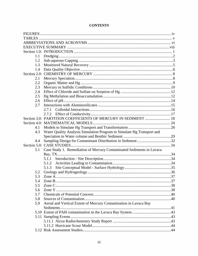
FIGURES....................................................................................................................................... iv TABLES ......................................................................................................................................... v ABBREVIATIONS AND ACRONYMS...................................................................................... vi EXECUTIVE SUMMARY ......................................................................................................... viii Section 1.0: INTRODUCTION ..................................................................................................... 1

1.1 Dredging .....................................................................................................................2 1.2 Sub-aqueous Capping .................................................................................................3 1.3 Monitored Natural Recovery ......................................................................................5 1.4 Data Quality Objective ...............................................................................................6

Section 2.0: CHEMISTRY OF MERCURY ................................................................................. 8 2.1 Mercury Speciation.....................................................................................................8 2.2 Organic Matter and Hg ...............................................................................................9 2.3 Mercury in Sulfidic Conditions ................................................................................10 2.4 Effect of Chloride and Sulfate on Sorption of Hg ....................................................12 2.5 Hg Methylation and Bioaccumulation ......................................................................12 2.6 Effect of pH...............................................................................................................14 2.7 Interactions with Aluminosilicates ...........................................................................15

2.7.1 Colloidal Interactions....................................................................................16 2.7.2 Effect of Conductivity...................................................................................17

Section 3.0: PARTITION COEFFICIENTS OF MERCURY IN SEDIMENT .......................... 18 Section 4.0: MATHEMATICAL MODELS................................................................................ 24

4.1 Models to Simulate Hg Transport and Transformation ............................................26 4.3 Water Quality Analysis Simulation Program to Simulate Hg Transport and

Speciation in Water column and Benthic Sediment .................................................29 4.4 Sampling Design for Contaminant Distribution in Sediment ...................................32

Section 5.0: CASE STUDIES...................................................................................................... 34 5.1 Case Study 1. Remediation of Mercury Contaminated Sediments in Lavaca

Bay, TX.....................................................................................................................34 5.1.1 Introduction - Site Description......................................................................34 5.1.2 Activities Leading to Contamination ............................................................34 5.1.3 Site Conceptual Model - Surface Hydrology................................................35

5.2 Geology and Hydrogeology......................................................................................36 5.3 Zone A ......................................................................................................................37 5.4 Zone B.......................................................................................................................37 5.5 Zone C.......................................................................................................................38 5.6 Zone Y ......................................................................................................................38 5.7 Chemicals of Potential Concern................................................................................40 5.8 Sources of Contamination.........................................................................................40 5.9 Aerial and Vertical Extent of Mercury Contamination in Lavaca Bay

Sediments..................................................................................................................41 5.10 Extent of PAH contamination in the Lavaca Bay System ........................................43 5.11 Sampling Events .......................................................................................................43

5.11.1 Alcoa Radiochemistry Study Report ............................................................43 5.11.2 Hurricane Scour Model.................................................................................44

5.12 Risk Assessment Studies...........................................................................................44

iv

5.12.1 Mercury Speciation is Sediments..................................................................46 5.13 Risk Characterization................................................................................................46 5.14 Ecological Risk Assessment .....................................................................................47 5.15 Remedial Action Objectives .....................................................................................48

5.15.1 Lavaca Bay....................................................................................................48 5.15.2 Chlor Alkali Process Area ............................................................................50 5.15.3 Witco.............................................................................................................50

5.16 Selected Remedies for the treatment of Lavaca Bay sediments ...............................50 5.16.1 Installation of a DNAPL Collection or Containment System at the

Witco Area ....................................................................................................50 5.16-2 Dredging of the Witco Channel ....................................................................50 5.16.3 Remediation of the Witco Marsh by Dredging.............................................51 5.16.4 Enhanced Natural Recovery North of Dredge Island ...................................51 5.16.5 Natural Recovery of Sediments ....................................................................51 5.16.6 Monitoring ....................................................................................................51 5.16.7 Removal of Building R-300 and Capping the Area......................................51 5.16.8 Capping of the Witco Soil.............................................................................52 5.16.9 Institutional Controls to Manage Exposure to Finfish/Shellfish...................52 5.16.10 Institutional Controls to Manage Exposure to Soil...................................52

5.17 Lessons Learned........................................................................................................53 5.18 Case Study 2. Sediment Stability Model to Empirically Determine Mercury

Budget in Onondaga Lake, New York......................................................................54 5.18.1 Methods for Estimating the Internal Fluxes of Internal Loads of HgT ........56

5.19 Summary ...................................................................................................................58 5.20 Case Study 3. Remediation and Monitoring of Mercury Contaminated

Sediments in Lake Turingen, Sweden ......................................................................59 5.21 Background Information...........................................................................................59 5.22 Remedial Technologies.............................................................................................61 5.23 Conventional Dredging and Capping........................................................................61 5.24 Capping with Artificial Sediment .............................................................................62 5.25 Construction Quality Control (CQC) and Environmental Monitoring (EM) ...........63 5.26 Results.......................................................................................................................64

Section 6.0: REFERENCES ........................................................................................................ 68

FIGURES

Figure 2-1. Aqueous Speciation Diagram of Hg(II) as Function of pH ........................................ 8 Figure 2-2. Sulfur Cycle in Freshwater Sediments...................................................................... 11 Figure 3-1. Sorption and Aging Processes Metals in Sediment................................................... 18 Figure 3-2. Idealized Mercury Concentration Profile in a Cap and Sediment and Flux Relationships................................................................................................................................. 23 Figure 4-1. Mathematical Model Framework and Relationship Between Various Models ........ 24 Figure 5-1. Site Location Map..................................................................................................... 35 Figure 5-2. Potentiometric Surface (Zone B) and Bay Hydrodynamics Map ............................. 36 Figure 5-3. Geological Sub-Units: I, II, III, IV, V, VI, and VII .................................................. 39

v

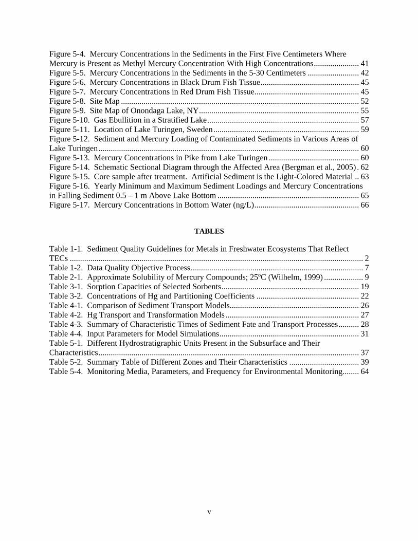
Figure 5-4. Mercury Concentrations in the Sediments in the First Five Centimeters Where Mercury is Present as Methyl Mercury Concentration With High Concentrations...................... 41 Figure 5-5. Mercury Concentrations in the Sediments in the 5-30 Centimeters ......................... 42 Figure 5-6. Mercury Concentrations in Black Drum Fish Tissue................................................ 45 Figure 5-7. Mercury Concentrations in Red Drum Fish Tissue................................................... 45 Figure 5-8. Site Map .................................................................................................................... 52 Figure 5-9. Site Map of Onondaga Lake, NY.............................................................................. 55 Figure 5-10. Gas Ebullition in a Stratified Lake.......................................................................... 57 Figure 5-11. Location of Lake Turingen, Sweden....................................................................... 59 Figure 5-12. Sediment and Mercury Loading of Contaminated Sediments in Various Areas of Lake Turingen............................................................................................................................... 60 Figure 5-13. Mercury Concentrations in Pike from Lake Turingen ............................................ 60 Figure 5-14. Schematic Sectional Diagram through the Affected Area (Bergman et al., 2005) . 62 Figure 5-15. Core sample after treatment. Artificial Sediment is the Light-Colored Material .. 63 Figure 5-16. Yearly Minimum and Maximum Sediment Loadings and Mercury Concentrations in Falling Sediment 0.5 – 1 m Above Lake Bottom ..................................................................... 65 Figure 5-17. Mercury Concentrations in Bottom Water (ng/L)................................................... 66

TABLES

Table 1-1. Sediment Quality Guidelines for Metals in Freshwater Ecosystems That Reflect TECs ............................................................................................................................................... 2 Table 1-2. Data Quality Objective Process.................................................................................... 7 Table 2-1. Approximate Solubility of Mercury Compounds; 25ºC (Wilhelm, 1999) ................... 9 Table 3-1. Sorption Capacities of Selected Sorbents................................................................... 19 Table 3-2. Concentrations of Hg and Partitioning Coefficients .................................................. 22 Table 4-1. Comparison of Sediment Transport Models............................................................... 26 Table 4-2. Hg Transport and Transformation Models ................................................................. 27 Table 4-3. Summary of Characteristic Times of Sediment Fate and Transport Processes.......... 28 Table 4-4. Input Parameters for Model Simulations.................................................................... 31 Table 5-1. Different Hydrostratigraphic Units Present in the Subsurface and Their Characteristics............................................................................................................................... 37 Table 5-2. Summary Table of Different Zones and Their Characteristics .................................. 39 Table 5-4. Monitoring Media, Parameters, and Frequency for Environmental Monitoring........ 64

vi

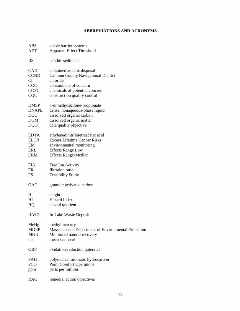
ABBREVIATIONS AND ACRONYMS

ABS active barrier systems AET Apparent Effect Threshold BS benthic sediment CAD contained aquatic disposal CCND Calhoun County Navigational District Cl chloride COC contaminate of concern COPC chemicals of potential concern CQC construction quality control DMSP 3-dimethylsulfone-propionate DNAPL dense, nonaqueous-phase liquid DOC dissolved organic carbon DOM dissolved organic matter DQO data quality objective EDTA ethylenedinitrilotetraacetic acid ELCR Excess Lifetime Cancer Risks EM environmental monitoring ERL Effects Range Low ERM Effects Range-Median FIA Free Ion Activity FR filtration ratio FS Feasibility Study GAC granular activated carbon H height HI Hazard Index HQ hazard quotient ILWD In-Lake Waste Deposit MeHg methylmercury MDEP Massachusetts Department of Environmental Protection MNR Monitored natural recovery msl mean sea level ORP oxidation-reduction potential PAH polynuclear aromatic hydrocarbon PCO Point Comfort Operations ppm parts per million RAO remedial action objectives

vii

RfD reference dose RI Remedial Investigation ROD record of decision RUSS Remote Underwater Sampling Station SHE Standard Hydrogen Electrode SSAS suspended solids and sediments TECs threshold effect concentrations TDS total dissolved solids TOC total organic carbon TSS total suspended solids UFI Upstate Freshwater Institute U.S. EPA United States Environment w/w wet weight WASP Water Quality Analysis Simulation Program

viii

EXECUTIVE SUMMARY Mercury is persistent in the environment. Though effort has been made in recent years to decrease mercury emissions into the environment, historically emitted mercury, adsorbed mainly by sediment, is still a dangerous threat to aquatic organisms, animals and even humans. Even if source control of contaminated wastewater is achievable, it may still take a very long time, perhaps centuries, for mercury-contaminated aquatic systems to reach relatively safe mercury levels in both water and surface sediment naturally (Chattopadhyay, 2005). It may take even longer to reduce mercury levels in deep sediment. Contaminated sediment results from Hg contamination persisting in the environment due to previous releases or due to ongoing contributions from sources that are difficult to identify. Due to human activities or natural processes, e.g., hydrodynamic flows, bioturbation, molecular diffusion, and chemical transformation, the buried mercury can be remobilized into the overlying water. Proper environmental management procedures, source control, contaminated sediment remediation, or their combination, are the usual options for cleaning up Hg-contaminated sites. The present report discusses the most common methods used for remediating contaminated sediment, the chemistry of mercury and its effect on the sorption of mercury on the sediment. The report also discusses some of the available mathematical models available to predict the fate and transport of mercury in the environment. Finally, the report presents several case studies. The first case study discusses the remediation efforts made at Lavaca Bay, Texas, where past activities have led to contamination of sediment. The second case is on the management of mercury present in Onandoga Lake in Syracuse, New York, and the third case study is on remediation and monitoring of mercury contaminated sediments in Lake Turingen, Sweden.

1

Section 1.0: INTRODUCTION Mercury can accumulate in the sediment from point and non-point sources, depending on a number of physical, chemical, biological, geological and anthropogenic environmental processes (Benoit et al., 1999; Braga et al., 2000; Hylander et al., 2000). It is believed that the associated mercury contamination in aquatic systems can be decreased by imposing effective management and monitoring strategies of contaminated sediment. Environmental project managers face several challenges in the management of contaminated sediment sites, primarily due to the large volumes of sediment that are typically involved. The complexities and high costs associated with characterization and cleanup are magnified by evolving regulatory requirements and the difficulties inherent in tracking the contaminants in the aquatic environments. Presently, four basic options for remediation of contaminated sediments exist for the environmental project managers, and they are:

(1) Containment in-place, (2) Treatment in-place, (3) Removal and containment, and (4) Removal and treatment.

Existing technologies for remediating mercury-contaminated sites focus primarily on highly polluted areas, and are not suitable for remediating vast, diffusely polluted sediment areas where pollutants occur at relatively low concentrations. Common mercury-contaminated sediment remediation strategies include dredging, capping and natural attenuation. Since each remedial action can result in a change in the physical, chemical and biological conditions of the sediment, it is expected that the speciation and transport properties of mercury might change as the result of implementing a remedial action. However, the effectiveness of such remediation practices have not been adequately assessed and long-term reliability has not been proven (Degetto et al., 1997). Though under the Clean Water Act, United States Environmental Protection Agency (U.S. EPA) has set recommended water quality criteria to protect human health and aquatic life, no target level is yet set for sediments. Long and Morgan (1991) evaluated a wide variety of marine sediment toxicity studies that were conducted in laboratory and field for the effects of sediment concentrations on benthic organisms. They established Effects Range-Low (ERL) and Effects Range-Medium (ERM) concentrations for each constituent evaluated. The ERL indicates the lower 10 percentile toxicity value in the database, and the ERM is the median toxicity value. They reported the ERL for total mercury as 0.15 milligram per kilogram (mg/kg) as dry weight (dry wt), and the ERM for total mercury as 1.3 kilogram per kilogram (kg/kg). Similar criteria for freshwater sediment are also proposed by Canada: a threshold effect level of 0.174 mg/kg (dry wt.) and a probable effect level of 0.486 mg/kg (Smith et al., 1996). Another example where screening criteria has been set is the adoption of consensus-based threshold effect concentrations (TECs) for the 28 chemicals, including mercury, by Massachusetts Department of Environmental Protection (MacDonald et al., 2000) for use in screening freshwater sediment for determining risk to benthic organisms. The TECs are intended to identify contaminant concentrations below which harmful effects on sediment-dwelling organisms are not expected. These concentrations may not necessarily be protective of higher level organisms exposed to bioaccumulating chemicals. This consensus-based TEC values were chosen as they incorporate a large data set, provide an estimate of central tendency that is not unduly affected by extreme values, and incorporate sediment quality guidelines that represent a number of approaches for developing sediment benchmarks (MDEP, 2002). A list of these consensus-based TECs is provided in Table 1-1.

2

Table 1-1. Sediment Quality Guidelines for Metals in Freshwater Ecosystems That Reflect TECs (MDEP, 2002)

Substance Consensus-Based TEC Metals (mg/kg) Arsenic 9.79 Cadmium 0.99 Chromium 43.4 Copper 31.6 Lead 35.8 Mercury 0.18 Nickel 22.7 Zinc 121

Brief descriptions of the common sediment remediation technologies are given below. Project managers should evaluate and compare the effectiveness of in-situ (capping and monitored natural recovery) and ex-situ (dredging) technologies under the conditions present at the site. The remediation selection criteria are dependent on site-specific conditions that constitute acceptable level of effectiveness and performance. 1.1 Dredging Dredging is the most common process used to remove the contaminated benthic sediments (Barbosa and Soares de Almeida, 2001). Dredging appears to be an effective remedy for systems heavily contaminated with mercury. One of the best example of dredging was Japan’s Minamata Bay, where mercury concentrations as high as 600 mg/kg was detected in settled sediment (Hosokawa, 1993). Dredging began in 1977 and ended in 1990. Based upon the report by Hosakawa (1993), monitoring data showed that at most sampling points, mercury concentrations were found to be below 5 mg/kg after dredging. Samples collected during and after dredging showed that mercury concentrations in water and fish were all below the safety requirement. Additionally, careful implementation of dredging did not have any significant adverse effect on the environment from sediment resuspension. Despite the results seen at Minamata Bay, dredging activities may cause adverse environmental threats if they are not well planned and implemented (Nichols et al., 1990; Schultz et al., 1995; Van Den Berg et al., 2001). Dredging-induced sediment re-suspension is a major environmental concern. Given no significant disturbance, buried mercury and other metals are generally sorbed by sediment, and can generally be regarded as safely separated from the overlying water. Activities such as dredging, shipping, and natural occurrences, such as storms and tides, can remobilize mercury that was sorbed by sediment (Van Den Berg et al., 2001). Bloom and Loasorsa (1999) conducted a laboratory experiment mimicking ocean dredging. They reported that about 5% of MeHg and less than 1% of total mercury can be released from contaminated sediment as a result of dredging. It is also noteworthy that sediment pore water, which usually contains high concentrations of mercury, can readily release mercury into the overlying water (Gilmour et al., 1992). After comparing different dredging techniques, Wang et al. (2004) suggested that a combination of mechanical and hydraulic dredging produces the least sediment re-suspension (Hauge et al., 1998). Mathematical models were developed to estimate dredging costs, efficiency, and environmental effects (Hayes et al., 2000; Blazquez et al., 2001). During dredging, oxygen in overlying water can enter buried anoxic sediment and possibly oxidize and release contaminants (Vale et al., 1998). Under undisturbed conditions, the formation of MeHg is restricted primarily to the uppermost 10 cm of

3

benthic sediment. Concentrations of MeHg are usually insignificant in the lower sediment (Gilmour et al., 1992; Bloom et al., 1999). However, it has been observed that after dredging, some buried sediment is mixed with surface sediment, or water, which can produce an environment with high sulfate and organic matter concentrations that favor the production of MeHg (Bloom and Loasorsa, 1999). Studies conducted in England showed that water discharged from dredging sites had higher concentrations of organic matter that favors the production of MeHg (Newell et al., 1999). One must note that dredging of the contaminated sediment is only a temporary solution to the problem (Barbosa and Soares de Almeida, 2001). The treatment of dredged sediment is usually very costly. Therefore, confinement (disposal followed by capping) and direct disposal are more common alternatives (Wang et al., 2004). The two most widely used disposal sites are land and sea water (Barbosa and Soares de Almeida, 2001). It is important to be aware of the fact that the disposal of dredged sediments poses a potential threat to the surrounding environment. Increased turbidity is usually observed at the dredge disposal sites (Nichols et al., 1990). The leakage of mercury into groundwater systems from disposal sites is another concern. In Georgia, the lower Savannah River showed elevated concentrations of some metals (including mercury) in living organisms close to an upland dredge disposal site (Winger et al., 2000). Contaminated dredged sediment confinement is widely used to prevent potential adverse environmental effects from dredge disposal. Adjusting pH to an optimal level is a common method to immobilize heavy metals. It is noteworthy that adding materials containing iron is also quite effective in immobilizing some heavy metals, such as cadmium and zinc, in dredged sediment. All contaminated dredged sediment should be properly treated before disposal. The very high cost of dredging is another limitation. It has been reported that the cost of active contaminated sediment remediation, including environmental dredging, could be as high as $1409/m3 (Cushing, 1999). As a summary, dredging can be very effective in cleaning up heavily mercury-contaminated sediment. However, it has disadvantages and concerns that need to be carefully addressed first, such as sediment re-suspension, oxidation change, disposal method, and cost.

1.2 Sub-aqueous Capping

Capping refers to the process of placement of a subaqueous covering or proper isolating materials to cover and separate the contaminated sediments from the water column. Cap can reduce risk of contamination by:

(1) physical isolation of the contaminated sediment from the aquatic environment, (2) stabilization/erosion protection of contaminated sediment, and (3) chemical isolation/reduction of the movement of dissolved and colloidally transported

contaminants into the water. In situ capping is on site placement of proper covering material over contaminated sediment in aquatic systems. Laboratory research suggests that in situ capping can be effective in reducing the impact of mercury contamination in aquatic systems. In ex situ capping, contaminated sediment is dredged and relocated to another site, where one or multiple isolating layers are placed over the sediment (Palermo, 1998; Liu et al., 2001). Ex situ capping is a combination of dredging and capping. Important distinctions should be made between in-situ capping and dredged material capping or ex-situ capping, which involves removal of sediments and placement at a subaqueous site, followed by placement of a cap. Dredged material capping is a disposal alternative which has been used for sediments dredged from navigation projects, and may also be suitable for disposal of sediments and treatment residues from remediation projects. There are two forms of dredged material capping: (a) level bottom capping, where a mound of dredged material is capped, and (b) contained aquatic disposal (CAD) in which dredged material is placed in a depression or other areas that provide lateral confinement prior to

4

placement of the cap. A considerable body of literature exists on the subject of sub-aqueous capping (Palermo et al., 1998; Truitt et al 1989; Sturgis and Gunnison 1988; Zeman et al., 1992). The cap may be constructed of clean sediments, sand, gravel, or may involve a more complex design with geotextiles, liners and multiple layers. A variation on cap could involve the removal of contaminated sediments to some depth, followed by capping the remaining sediments in-place. This is suitable where capping alone is not feasible because of hydraulic or navigation restrictions on the waterway depth. Experimental tests show that the capping material, composed of a mixture of sand and finer particles (silty sands as per ASTM classification), can adsorb mercury and other heavy metals (Moo-Young et al., 2001). Moo-Young et al. (2001) showed that capping materials can adsorb 99.9% of the mercury from sediment, which contained mercury between 200 and 500 microgram per liter (µg/L). This test showed that a capping layer can be a good barrier between mercury-contaminated sediment and the overlying water. In situ capping field studies were conducted in Hamilton Harbour, Canada, which has high concentrations of zinc, copper, mercury, and other metals. A cap, approximately 35 cm thick and composed mostly of sand, was placed in the system to contain polluted sediment (Azcue et al., 1998). After one year of in situ capping, a field study investigated the effectiveness of the cap. In general, mercury concentrations were found to be low (less than 5 microgram per kilogram [µg/kg]) in the capping layer, while the concentration of mercury in the original sediment ranged between 0.43 and 0.96 gram per kilogram (g/kg) (Azcue et al., 1998). This result suggests that a capping layer can contain mercury in the original sediment. In aquatic systems, mercury is in various forms, and some forms may have a stronger tendency to attach to sediment than others. For example, inorganic mercury is more likely to attach to sediment than organic mercury. Activity of inorganic mercury deep within the sediment is generally low. The major advantages of in situ capping are low cost, extensive suitability to a wide range of contaminants, and low adverse environmental effects (Azcue et al., 1998; Palermo, 1998). As in situ capping is not a treatment process, long-term environmental effects, including possible remobilization of contaminated sediment, need to be carefully considered by regular monitoring of the capped system. However, there is a possibility that buried mercury may pass through the capping layer and enter into the overlying water due to various reasons (hydrodynamic flows, consolidation, transformation, diffusion, etc.). Hydrodynamic currents caused by human activities or natural processes, such as shipping, tide, and groundwater flow, may scour the capping layer and release mercury into the water. For example, laboratory experiments suggest that sub-aqueous groundwater flow reduces the efficiency of capping significantly (Liu et al., 2001). The movement of benthic organisms may also facilitate the remobilization of buried mercury. Sediment consolidation, due to gravity, can move mercury from buried sediment into the capping layer. This sediment consolidation may be a more important factor in the transfer of mercury from buried sediment into the capping layer than molecular diffusion of mercury (Moo-Young et al., 2001). Though a pilot test conducted in a Canadian harbor suggested no significant sediment re-suspension due to capping (Hamblin et al., 2000), there is always the possibility of re-suspension of originally settled sediment due to the placement of the capping layer. Such re-suspension can be the cause for transforming some of the inorganic mercury into organic mercury (MeHg) through biological processes. MeHg can escape into the overlying water more easily than inorganic mercury. Site characterization is the preliminary and crucial step to decide whether a contaminated aquatic system is suitable for capping. In general, aquatic environments with low hydrodynamic flows, such as lakes and bays, are good candidates for capping (Thoma et al., 1993). The type of capping material can be used depends on the hydrodynamic, geotechnical conditions, and target contaminants. Sand and other fine materials are good for quiescent environments (Palermo, 1998). For erosive systems,

5

coarser materials should be considered (Palermo, 1998). Jacobs and Forstner (1999) proposed the idea of using active barrier systems (ABS) with in situ capping. Zeolite is a good candidate for applying in situ capping with ABS (Jacobs and Forstner, 1999). ABS usually is a reactive geochemical barrier layer that can actively block the contaminant release from the sediment entering into the overlying water, without the hydraulic contact between the sediment and the overlying water being disturbed (Jacobs and Forstner, 1999). In situ capping with ABS adsorbs target constituents from the sediment and prevents the release of target contaminants into the overlying water more effectively than in situ capping alone. 1.3 Monitored Natural Recovery Monitored natural recovery (MNR) is a remedial technology for contaminated sediments that typically uses ongoing, naturally occurring processes to contain, destroy, or reduce the bioavailability or toxicity of contaminants in sediment (Khan and Husain, 2002). These processes may include physical, biological, and chemical mechanisms that act together to reduce risk posed by contaminants. The key factors that dictate the selection of MNR as a remedial technology are the concentrations of constituents of concern and whether they pose an unacceptable risk, any ongoing degradation/transformation, or dispersion of contaminant, and the establishment of a cleanup level that MNR is expected to meet within a particular time frame. The sites, which are ecologically sensitive in nature and where mercury is strongly bound to the sediments, are reasonable candidates for using MNR as the remedial technology. This would involve monitoring for mercury movement in the aqueous phase. Detailed spectroscopic study of the nature of the mercury in solid phases and the environmental conditions conducive to their dissolution is necessary to define the necessary safeguards to impose on the site for successfully implementing MNR. As it is generally considered that the solid phases that hold mercury are themselves sensitive to the state of oxidation-reduction (Fe-oxide or sulfide phases), institutional controls would have to be imposed to safeguard the site from extreme fluxes of oxidation-reduction potential. This may involve protecting the site from extremely oxidizing conditions, which may result from water being directed away from or drained from the site. Such conditions may promote the dissolution of sulfide precipitates and the degradation of organic matter. Conversely, institutional controls may involve protecting the site from extremely reducing conditions, which may result from sustained flooding conditions that may cause Fe(III)-oxide phases to dissolve. The two primary advantages of MNR are its relatively low implementation cost and its non-invasive nature that does not need construction/infrastructure. Though costs associated with characterization and/or modeling to evaluate natural recovery can be extensive, the primary cost associated with implementing MNR is monitoring. The other advantages of MNR over active remedial methods include no sediment resuspension, and no change in benthic conditions (Garbaciak et al., 1998). The key limitations of MNR may be the potential risk of re-exposure or dispersion of buried Hg if the sediment bed is disturbed by strong natural or man-made forces and uncertainties in predicting various situations, like, future sedimentation rates in dynamic environments, rate of contaminant flux through stable sediment, or rate of natural recovery. Contaminated systems in natural attenuation should be regularly monitored to ensure environmental safety. Experiments and field studies demonstrate possible natural attenuation of mercury contamination by reduction, demethylation, and volatilization. Two important ways to naturally reduce Hg(II) in surface waters are photoreduction and microbial reduction. In low mercury concentrations (low picomolar range), photoreduction is more effective than microbial reduction (Amyot et al., 1997). Morel et al.(1998) reported that at high mercury concentrations (over 50 picomole), microbial reduction is more effective and in deep anoxic environments, certain bacteria in the presence of humic substances reduces Hg(II). Microbial demethylation of MeHg was observed in contaminated sediment (Oremland et al., 1995; Marvin-Dipasquale and Oremland, 1998). Sulfate-reducing bacteria and methanogenic bacteria are probable agents in microbial demethylation (Oremland et al., 1995). Total Hg concentration and organic

6

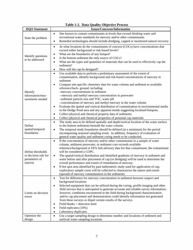
substance content are important factors in microbial demethylation (Marvin-Dipasquale et al., 2000). A demethylation rate ranged from 0.02 to 0.5 ng/g (dry sediment) per day in a field study (Marvin-Dipasquale and Oremland, 1998). Photodegradation of MeHg can also happen in surface waters (Sellers et al., 1996). Photodegradation of MeHg seems to be a first-order reaction with respect to MeHg concentration and sunlight intensity (Sellers et al., 1996). In aquatic systems, Hg0 volatilization plays an important role in the natural attenuation of mercury contamination (Amyot et al., 1997). Hg0 is probably the end-product of some reduction processes of MeHg and Hg(II) (Sellers et al., 1996). Due to its high volatility, Hg0 produced by the reduction of MeHg and Hg(II) rapidly evaporates into the atmosphere. This evaporation is a major natural attenuation of mercury in some aquatic systems. Garbaciak et al. (1998) reported field experiments performed in the Whatcom Waterway at Bellingham, Washington, using natural attenuation of mercury-contaminated aquatic systems. In the 1960s, the mercury concentration in the surface sediment was about 4.5 mg/kg. After source control and natural attenuation, mercury concentration in the surface sediment was reduced to about 0.5 mg/kg. Garbaciak et al. (1998) also defined enhanced natural attenuation as natural decontamination, accelerated by human influences. Garbaciak et al. (1998) reported the result of enhanced natural attenuation of Hg-contaminated Eagle Harbor site, Washington. A thin clean sediment cap (6 cm) was placed on the contaminated sediment to enhance the burial and separation effects, because the natural sedimentation process was too slow. These authors reported that compared to thick capping, this enhanced natural attenuation method of thin capping did not change the benthic environment significantly. However, due to the strong persistence of mercury in the environment, it may take a long time for heavily contaminated aquatic systems to fully recover through natural attenuation. 1.4 Data Quality Objective Data quality objectives (DQOs) are statements that specify the quantity and quality of the data required to support project decisions. The process as defined by the U.S. EPA (U.S. EPA, 2000) was used to plan the approach for collecting the necessary data to meet the objectives of a study. The seven-step process is summarized in Table 1-2. The quality control procedures as well as the associated field sampling procedures for a project need to be focused on achieving these DQOs in a timely, cost-effective, and safe manner. Deviations from the DQOs may require defining the cause or causes for noncompliance and will initiate the process of determining whether additional sampling and analyses will be necessary to attain project goals.

7

Table 1-2. Data Quality Objective Process DQO Statement Issues/Concerns/Information

State the problem • Site known to contain contaminants at levels that exceed drinking water and

recreational water standards for mercury and/or other contaminants • Remedial technologies should include dredging, capped or monitored natural recovery

Identify questions to be addressed

• At what locations do the contaminants of concern (COCs) have concentrations that exceed either background or risk-based levels?

• What are the boundaries of any hotspot? • Is the bottom sediment the only source of COCs? • What are the types and quantities of materials that can be used to effectively cap the

sediment? • How will the cap be designed?

Identify information/mea-surements needed

• Use available data to perform a preliminary assessment of the extent of contamination, identify background and risk-based concentrations of mercury in sediment

• Compare site-specific chemistry data for water column and sediment to available reference/back- ground, including: –mercury concentrations in sediment –-mercury and methyl mercury concentration in porewater –sediment particle size and TOC, water pH –concentrations of mercury and methyl mercury in the water column

• Evaluate the spatial and vertical distribution of contamination in environmental media in the Dodge Pond area and any apparent trends suggesting localized hotspots.

• Collect physical and chemical property data of sediments • Collect physical and chemical properties of potential cap materials

Define spatial/temporal boundaries

• The study area to be defined spatially and depth/vertical location of the water surface to the bottom sediments beneath the water column.

• The temporal study boundaries should be defined (at a minimum) for the period encompassing seasonal sampling event. In addition, frequency of evaluation of general water quality and sediment coring needs to be conducted.

Define thresholds or decision rule for parameters of interest

• If the concentration of mercury and/or other contaminants in a sample of water column, sediment porewater, or sediment core exceeds available reference/background or EPA fish advisory data for that contaminant, the contaminant will be considered a COPC.

• The spatial/vertical distribution and identified gradients of mercury in sediment and water before and after placement of cap (or dredging) will be used to determine the overall performance and extent of remediation of mercury.

• If hot spot area identified by past bathymetric study used for application of cap, exploratory sample cores will be collected to characterize the nature and extent (spread) of mercury contamination in the sediments.

Limits on decision errors

• Test for difference for mercury concentration in sediment between suspect and background locations

• Selected equipment that can be utilized during the coring, profile imaging and other field surveys that is anticipated to generate accurate and reliable survey information; however, conditions encountered in the field during background characterization and/or cap placement and demonstration could identify information not generated from these surveys or dispel certain results of the surveys.

• Field blanks < detection limit • Field replicates (10%) • Laboratory duplicates

Optimize the design

• Use a target sampling design to determine number and locations of sediment and surficial water sampling locations

8

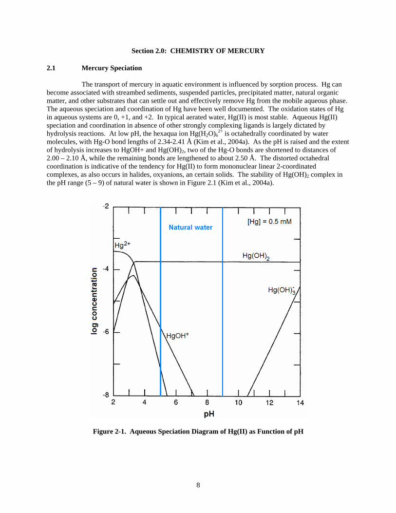
Section 2.0: CHEMISTRY OF MERCURY 2.1 Mercury Speciation The transport of mercury in aquatic environment is influenced by sorption process. Hg can become associated with streambed sediments, suspended particles, precipitated matter, natural organic matter, and other substrates that can settle out and effectively remove Hg from the mobile aqueous phase. The aqueous speciation and coordination of Hg have been well documented. The oxidation states of Hg in aqueous systems are 0, +1, and +2. In typical aerated water, Hg(II) is most stable. Aqueous Hg(II) speciation and coordination in absence of other strongly complexing ligands is largely dictated by hydrolysis reactions. At low pH, the hexaqua ion Hg(H2O)6

2+ is octahedrally coordinated by water molecules, with Hg-O bond lengths of 2.34-2.41 Å (Kim et al., 2004a). As the pH is raised and the extent of hydrolysis increases to HgOH+ and Hg(OH)2, two of the Hg-O bonds are shortened to distances of 2.00 – 2.10 Å, while the remaining bonds are lengthened to about 2.50 Å. The distorted octahedral coordination is indicative of the tendency for Hg(II) to form mononuclear linear 2-coordinated complexes, as also occurs in halides, oxyanions, an certain solids. The stability of Hg(OH)2 complex in the pH range (5 – 9) of natural water is shown in Figure 2.1 (Kim et al., 2004a).

Figure 2-1. Aqueous Speciation Diagram of Hg(II) as Function of pH

9

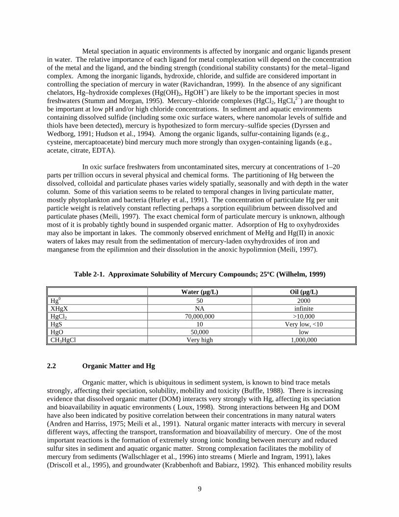
Metal speciation in aquatic environments is affected by inorganic and organic ligands present in water. The relative importance of each ligand for metal complexation will depend on the concentration of the metal and the ligand, and the binding strength (conditional stability constants) for the metal–ligand complex. Among the inorganic ligands, hydroxide, chloride, and sulfide are considered important in controlling the speciation of mercury in water (Ravichandran, 1999). In the absence of any significant chelators, Hg–hydroxide complexes (Hg(OH)2, HgOH+) are likely to be the important species in most freshwaters (Stumm and Morgan, 1995). Mercury–chloride complexes (HgCl2, HgCl4

2−) are thought to be important at low pH and/or high chloride concentrations. In sediment and aquatic environments containing dissolved sulfide (including some oxic surface waters, where nanomolar levels of sulfide and thiols have been detected), mercury is hypothesized to form mercury–sulfide species (Dyrssen and Wedborg, 1991; Hudson et al., 1994). Among the organic ligands, sulfur-containing ligands (e.g., cysteine, mercaptoacetate) bind mercury much more strongly than oxygen-containing ligands (e.g., acetate, citrate, EDTA). In oxic surface freshwaters from uncontaminated sites, mercury at concentrations of 1–20 parts per trillion occurs in several physical and chemical forms. The partitioning of Hg between the dissolved, colloidal and particulate phases varies widely spatially, seasonally and with depth in the water column. Some of this variation seems to be related to temporal changes in living particulate matter, mostly phytoplankton and bacteria (Hurley et al., 1991). The concentration of particulate Hg per unit particle weight is relatively constant reflecting perhaps a sorption equilibrium between dissolved and particulate phases (Meili, 1997). The exact chemical form of particulate mercury is unknown, although most of it is probably tightly bound in suspended organic matter. Adsorption of Hg to oxyhydroxides may also be important in lakes. The commonly observed enrichment of MeHg and Hg(II) in anoxic waters of lakes may result from the sedimentation of mercury-laden oxyhydroxides of iron and manganese from the epilimnion and their dissolution in the anoxic hypolimnion (Meili, 1997).

Table 2-1. Approximate Solubility of Mercury Compounds; 25ºC (Wilhelm, 1999)

Water (µg/L) Oil (µg/L) Hg0 50 2000 XHgX NA infinite HgCl2 70,000,000 >10,000 HgS 10 Very low, <10 HgO 50,000 low CH3HgCl Very high 1,000,000

2.2 Organic Matter and Hg Organic matter, which is ubiquitous in sediment system, is known to bind trace metals strongly, affecting their speciation, solubility, mobility and toxicity (Buffle, 1988). There is increasing evidence that dissolved organic matter (DOM) interacts very strongly with Hg, affecting its speciation and bioavailability in aquatic environments ( Loux, 1998). Strong interactions between Hg and DOM have also been indicated by positive correlation between their concentrations in many natural waters (Andren and Harriss, 1975; Meili et al., 1991). Natural organic matter interacts with mercury in several different ways, affecting the transport, transformation and bioavailability of mercury. One of the most important reactions is the formation of extremely strong ionic bonding between mercury and reduced sulfur sites in sediment and aquatic organic matter. Strong complexation facilitates the mobility of mercury from sediments (Wallschlager et al., 1996) into streams ( Mierle and Ingram, 1991), lakes (Driscoll et al., 1995), and groundwater (Krabbenhoft and Babiarz, 1992). This enhanced mobility results

10

in increased water column concentrations of mercury in otherwise pristine lakes and streams. Complexation also affects the partitioning of mercury to suspended solids in the water column and the sequestration of mercury to sediments. DOM is also known to promote (Weber, 1993) or inhibit ( Miskimmin, 1992) the formation of toxic and bioaccumulative methylmercury species. Complexation with DOM limits Hg(II) availability to methylating bacteria and CH3Hg+ availability for bioaccumulation (Barkay et al., 1997). Humic and fulvic acid fractions of DOM are also capable of reducing ionic mercury to the volatile elemental mercury (Alberts et al., 1974), increasing the reflux of mercury from water and soil to the atmosphere. More importantly, DOM enhances the formation of Hg0 from Hg(II) in photochemical reactions (Ravichandran, 2004), which could reduce the availability of mercury for methylation and bioaccumulation. 2.3 Mercury in Sulfidic Conditions Based on the preference of a cation for complexation with ligands, mercury is classified as a B-type metal cation, characterized by a “soft sphere” of highly polarizable electrons in its outer shell. Soft metals like mercury show a pronounced preference for ligands of sulfur, the less electronegative halides, and nitrogen over ligands containing oxygen (Stumm and Morgan, 1995). From an ecological consideration, Halbach (1995) concluded that the bioaccumulation of mercury in fish and its toxicity in humans is attributed to the high affinity of mercury for sulfur-containing proteins such as metallothionein and glutathione. Strong interactions between mercury and organic matter found in sediment and aquatic environments are attributed to the binding of mercury with sulfur-containing functional groups in organic matter. Sulfur is a minor constituent in DOM, ranging from about 0.5% to 2.0% by weight. Sulfur in DOM occurs as reduced (e.g., sulfide, thiol) or as oxidized species (e.g., sulfonate, sulfate), with oxidation states ranging from −2 to +6. The stability constant for Hg2+ complexation with an oxidized sulfur ligand, SO4

2−, is 101.3, whereas, the stability constant for Hg2+ complexation with a reduced sulfur ligand, S2−, is 1052.4. The reduced sulfur sites are expected to be important for mercury binding. Generally, hydrophobic acid fractions of DOM (which includes the humic and fulvic acid fractions) had significantly higher reduced sulfur content than the low molecular weight hydrophilic acid fractions. Even if we assume that only a small fraction (about 2% as suggested by Amirbahman et al., 2002) of the reduced sulfur is available for binding with mercury in natural systems, the strong binding sites in organic matter far exceed the amount of mercury available in natural aquatic systems. Because binding of mercury to DOM under natural conditions is controlled by a small fraction of DOM molecules containing reactive thiol functional groups (Haitzer et al., 2002), a positive correlation may not always exist between Hg and dissolved organic carbon (DOC) concentration (Hurley et al., 1998). When mercury and DOC concentrations are poorly correlated in aquatic environments, it neither implies that organic matter is not important for Hg binding or transport, nor that organic matter interacts weakly with mercury. In general, positive correlation between Hg and DOC concentrations could be expected in cases where Hg is released and co-transported with the organic matter (Wallschlager et al., 1996). On the other hand, in systems where water column mercury is primarily derived from direct atmospheric sources, correlation between Hg and DOC may or may not be present. In both cases, significant differences can be expected in the reactivity of DOM with mercury depending on the structural and chemical characteristics of DOM (Babiarz et al., 2001) and the presence of other competing ions in water. Hasterberg et al. (2001) concluded that as S/Hg ratio increased, multiple sulfur ligands were coordinated with mercury. Ravichandran (2004) reported that the organic matter and mercaptoacetic acid (HS–CH2–COOH), a thiol-containing compound caused a dramatic increase in mercury release (up to 35 M total dissolved Hg) from cinnabar (HgS), a relatively insoluble solid (Ksp=10-36.8). DOM also inhibited

11

the precipitation of metacinnabar (black HgS), a very insoluble solid (Ksp=10-36.4), at an initial Hg concentration 5 × 10-8 M (Ravichandran, 2004). In contrast to sulfur-containing ligands, oxygen-containing ligands such as acetic acid and ethylenedinitrilotetraacetic acid (EDTA) dissolved very little or no mercury from cinnabar. Mercury speciation models calculated as a function of sulfide concentrations and pH suggest that HgSaq

0, Hg(S2H)-, Hg(SH)20, and HgSs are likely to be the most important species (Hurley et al.,

1994). Sulfur cycling (see Figure 2-2) in aquatic sediments involves both reductive and oxidative processes (Jørgensen, 1990) and they often play significant role in forming metal complexes.

Figure 2-2. Sulfur Cycle in Freshwater Sediments (modified after Holmer and Storkholm, 2001)

The stability constants for Hg–organic sulfur (HgRS+) complex are much lower than that for inorganic sulfide. The stability constants for these complexes are (Benoit et al., 1999; Dyrssen and Wedborg, 1991) indicated below.

Hg2+ + HS- ↔ HgSaq0 + H+ K=1026.5

Hg2+ + 2HS- ↔ Hg(S2H)- + H+ K=1032.0 Hg2+ + 2HS- ↔ Hg(SH)2

0 K=1037.5 Hg2+ + RS- ↔ HgRS+ K=1022.1

However, the Hg–DOM binding constants in natural environments are reported to be much higher. The binding constants for HgRS+ complex was determined at 1025.8 – 1027.2 by Drexel et al. (2002), 1028.5 by Haitzer et al. (2002), and 1031.6–1032.2 by Skyllberg et al. (2000). These values are higher than Hg complexation with inorganic sulfides. Differences between the above values may be attributed to

12

the Hg/DOM ratio in these studies, wherein mercury may be bound by a single RSH group, by bidentate aromatic and aliphatic thiols and phenols or carboxyls ( Xia et al., 1999; Hasterberg et al., 2001; Drexel et al., 2002). These high stability constants indicate that organic matter can easily out compete sulfide for the complexation of mercury in anoxic environments. 2.4 Effect of Chloride and Sulfate on Sorption of Hg The sorption of Hg onto particles can be significantly affected by the presence of complexing ligands, like chloride and sulfate that are present in freshwater or seawater. These ligands affect the sorption of Hg due to several possible processes including (a) formation of stable non-sorbing metal-ligand aqueous complexes; (b) formation of metal-ligand ternary surface complexed, which at high metal and ligand concentrations can lead to surface precipitation; (c) competitive ligand sorption to particle surfaces, effectively blocking the more reactive sorption sites at the surface; and (d) reduction of positive charge at particle surfaces, and thus lowering the electrostatic repulsion of cations by surfaces (considering ligands are anions and pH levels are below pHpzc of the mineral particles). Kim et al (2003) reported that presence of chloride and sulfate resulted reduction in sorption of Hg(II) on goethite (α-FeOOH), γ-alumina (γ-Al2O3), and bayerite (β-Al[OH]3), which are useful surrogates for the natural sediments. Over the chloride concentration range 10-5 to 10-2 M, the lowering in Hg sorption on α-FeOOH, γ-Al2O3, and β-Al(OH)3 were from 0.42 to 0.07 µmol/m2, 0.06 to 0.006 µmol/m2, and 0.55 to 0.39 µmol/m2, respectively. This reduction in Hg(II) sorption is primarily due to the formation of stable, non-sorbing aqueous HgCl2 complexes in solution, limiting the amount of free Hg(II) available to sorb. A higher chloride concentration (Cl- ≥ 10-3 M) and pH 6, the large proportion of unsorbed aqueous Hg(II) facilitated reduction of Hg(II) to Hg(I) and the formation of Hg2Cl2 (s) (calomel) or Hg2Cl2 (aq) species. Sulfate, in contrast, enhanced Hg(II) sorption over the sulfate concentration range 10-5 to 0.9 M, increasing Hg surface coverage on α-FeOOH, γ-Al2O3, and β-Al(OH)3 from 0.39 to 0.45 µmol/m2, 0.11 to 0.38 µmol/m2, and 0.36 to 3.33 µmol/m2, respectively. This effect might be due to the sorption or accumulation of sulfate ions at the substrate interface, effectively reducing the positive surface charge that electrostatically inhibits Hg(II) sorption. 2.5 Hg Methylation and Bioaccumulation In most freshwaters, the predominant form of mercury is ionic mercury in the divalent state (Hg[II]), whereas in most fish species >95% of mercury is in the form of monomethylmercury (CH3Hg). Thus, conversion of ionic mercury to methylmercury is an important link in the bioaccumulation of mercury in fish and ultimately its toxicity to humans and wildlife. Methylmercury production in sediment and aquatic systems is not a simple function of total mercury concentration in the system. Methylmercury formation is influenced by a number of environmental factors including temperature, pH, redox potential, activity and structure of bacterial community, and the presence of inorganic and organic complexing agents. Dissolved Hg is distributed among several chemical forms: elemental mercury (Hgaq

0), which is volatile but relatively non-reactive, a number of mercuric species (Hg[II]), and organic mercury, mainly methyl (MeHg), dimethyl (Me2Hg), and some ethyl (EtHg) mercury. In general, and particularly in stratified systems, concentrations of Hg0 are higher near the air-water interface whereas levels of total Hg and MeHg are higher near the sediments. Mercury methylation is mainly a microbially mediated process, with abiotic methylation likely to be important in organic-rich lakes (Ullrich et al., 2001). Bacteria assimilate mercury through passive diffusion of neutrally charged species ( Barkay et al., 1997) as well as by active uptake of both charged and uncharged mercury (Kelly et al., 2003). Wetland sediments commonly have a lower oxidation-reduction potential (ORP), or Eh, thereby promoting the reduction of Hg(II) to Hg(I) or Hg0.

13

Oxidation-reduction potentials influence Hg speciation through its affect on sulfur chemistry. Decreases in oxidation-reduction potential promote microbially mediated sulfur-reduction, which in turn promotes Hg methylation. Furthermore, the accumulation of reduced sulfur, primarily as dissolved sulfide, will precipitate inorganic Hg as a highly insoluble HgS mineral, cinnabar (red coloration) or meta-cinnabar (black and slightly more soluble). Increases in of dissolved sulfide concentrations result in decreases in Hg methylation rates because inorganic Hg is removed as a sparingly soluble solid (Gilmour et al. 1992). Finally, wetlands typically have very high concentrations of organic matter due to the slow rate of organic matter oxidative degradation occurring in this environment. The organic matter may either act as a sorbent or may provide high concentrations of dissolved ligands that form very strong complexes to Hg(II) (Cleam and Gamble 1974; Wallschlager et al. 1998). In microbial methylation, complexation with DOC generally limits the amount of inorganic mercury available for uptake by methylating bacteria (Kelly et al., 2003) because DOC molecules are generally too large to cross the cell membranes of the bacteria. DOM-mediated reduction of Hg(II) to the volatile Hg0 species would also reduce the bioavailability of mercury for methylation and subsequent biological uptake. The effect of DOC on mercury bioavailability may also be affected by the pH of the water column. At low pH, DOC is less negatively charged, and therefore less likely to complex mercury, making it more available to the methylating bacteria (Miskimmin et al., 1992; Barkay et al., 1997). In sulfate-limited environments where microbes may be utilizing organic matter as energy source, DOC may have a stimulating effect on microbial growth and thus enhance methylation rates in the water column and sediments (Watras et al., 1995). It may be hypothesized that where organic matter is largely labile and readily biodegradable, it may promote methylation by stimulating microbial growth, and when the organic matter is relatively recalcitrant and consists of high molecular weight humic and fulvic acids, then it may contribute to abiotic methylation. According to Stumm and Morgan (1995), the divalent mercury in surface waters, Hg(II), is not present as the free ion Hg2+ but should be complexed in variable amounts to hydroxide (Hg(OH)+, Hg(OH)2, Hg(OH)3

-), and to chloride (HgCl+, HgClOH, HgCl2, HgCl3-, HgCl4

2-) ions depending on the pH and the chloride concentration. Even in oxic surface waters, some or much of Hg(II) might be bound to sulfides. In addition, an unknown fraction of Hg(II) is likely bound to humic acids, the assemblage of poorly defined organic compounds that constitute 50–90% of the DOC in natural waters. According to Meili (1997), nearly 95% of inorganic oxidized mercury in lakes is bound to dissolved organic matter. Through its binding to DOC, Hg can be mobilized from the drainage basin and transported to lakes (Morel et al., 1998). The reactions of ionic mercury are relatively fast, and it is thought that the various species of Hg(II), including those in the particulate phase, are at equilibrium with each other. In the organometallic species of mercury, the carbon-to-metal bonds are stable in water because they are partly covalent and the hydrolysis reaction, which is thermodynamically favorable (and makes the organometallic species of most others metals unstable), is kinetically hindered. As a result, the dimethyl mercury species, Me2Hg (CH3HgCH3), is non-reactive. The monomethyl species, MeHg, is usually present as chloro- and hydroxocomplexes (CH3HgCl andCH3HgOH) in oxic water. Once methylmercury is formed, DOC facilitates its solubility, and thus increasing water column concentration) and transport through complexation (Miskimmin, 1991). At the same time, complexation with DOC also tends to limit its uptake in biota (Driscoll et al., 1995). Apart from DOC, concentration and bioaccumulation of MeHg in fish is also affected by pH, temperature, redox potential, concentrations of aluminum and calcium, fish age and food source, and other factors (Watras et al., 1995). Temperature and season influence the availability and accumulation of mercury in addition to the factors already discussed. Changes in temperature can affect mercury concentrations in organisms either directly by affecting metabolic rate and thereby exposure, or indirectly by influencing the methylation of mercury and therefore enhancing availability. Rates of methyl- or inorganic mercury uptake increase with increasing aqueous concentrations and/or increasing temperature in the water for some species such as, phytoplankton, gastropods, fish (Rodgers and Beamish, 1981; Tessier et al., 1994). A rise in temperature

14

(and a corresponding rise in respiratory volume) can increase the rate of uptake via the gills (U.S. EPA, 1985). The abiotic methylation increases with increase in temperature. An increase of the reaction temperature from 5ºC to 40ºC doubled the methyl mercury yields, as did the doubling of the spike concentration of the Hg2+ (Rogers, 1977). Biological productivity of methylating microbes is affected by seasonal changes in temperature, nutrient supply, oxygen supply, and hydrodynamics (changes in suspended sediment concentrations and flow rates). MeHg concentrations varied seasonally by an order of magnitude at most sites studied (Parks et al., 1989). Methylation may tend to increase during the summer months when biological productivity and temperature are high and decrease during winter months when biological productivity and temperature are low (Callister and Winfrey 1986; Kelly et al., 1995). Although the potential MeHg production is greatest during the summer, actual production may not peak during this time (Kelly et al., 1995). In Onondaga Lake, New York, the mercury species in the water column varied temporally (Battelle 1987; Bloom and Effler, 1990). Total mercury concentrations may also vary seasonally due to physical factors such as winter storms resuspending mercury-contaminated sediments (Gill and Bruland, 1990). Various abiotic reactions that could be responsible for abiotic mercury methylation are indicated below.

(1) Transalkylation reaction by other methylated metals like lead and arsenic. (2) Methylation by released methylcobalamine from bacteria. (3) Methylation by separate compounds due to cellular components like S-

adenosylmethionine, 3-dimethylsulfone-propionate (DMSP), methyl iodide, homocysteine, dimethylsulfide.

(4) Methylation by humic and fulvic acids and degradation products.

2.6 Effect of pH Neutral or low pH conditions favor the production of monomethylmercury over dimethylmercury (Beijer and Jernelov, 1979) and alkaline pH favors the formation of dimethylmercury (NOAA, 1996). The pH range for inorganic mercury methylation was reported to be between pH 5.5 and pH 2 (Falter, 1999). Kelly et al. (2003) studied the effect of increasing hydrogen ion (H+) concentration on the uptake of mercury (Hg[II]) by an aquatic bacterium. Even small changes in pH (7.3-6.3) resulted in large increases in Hg(II) uptake, in defined media. The increased rate of bioaccumulation was directly proportional to the concentration of H+. Lowering the pH of Hg solutions mixed together with natural dissolved organic carbon, or with whole lake water, also increased bacterial uptake of Hg(II). Using both defined inorganic solutions and lake water, uptake of Hg(II) was faster at lower pH, and the increased rate of uptake was not related to changes in neutral Hg species such as HgCl2 or Hg(OH)2. Rather, uptake of both charged and uncharged Hg(II) species appeared to increase as H+ increased, indicating a facilitated bacterial Hg(II) uptake process that responds to pH. Hg(II) uptake rate by bacteria (for example, Vibrio anguillarum) under aerobic or anaerobic conditions is controlled by the collective concentration of a number of available Hg(II) species, both charged and uncharged, which indicates that a cell-mediated process is important in determining how much Hg(II) enters the cell. In addition to the bacterial Hg(II) uptake process, an increase in bioavailable mercury concentration at reduced pH conditions is due to the desorption of Hg(II) from DOC or particles, which is expected because H+ can displace Hg(II) by protonating sulfhydryl moieties that bind Hg (II) to DOC (Benoit et al., 1999) or by replacing Hg(II) on negatively charged surfaces such as clays (aluminosilicates).

15

Generation of MeHg in Anoxic Sediment and Water Systems, and Transportation by

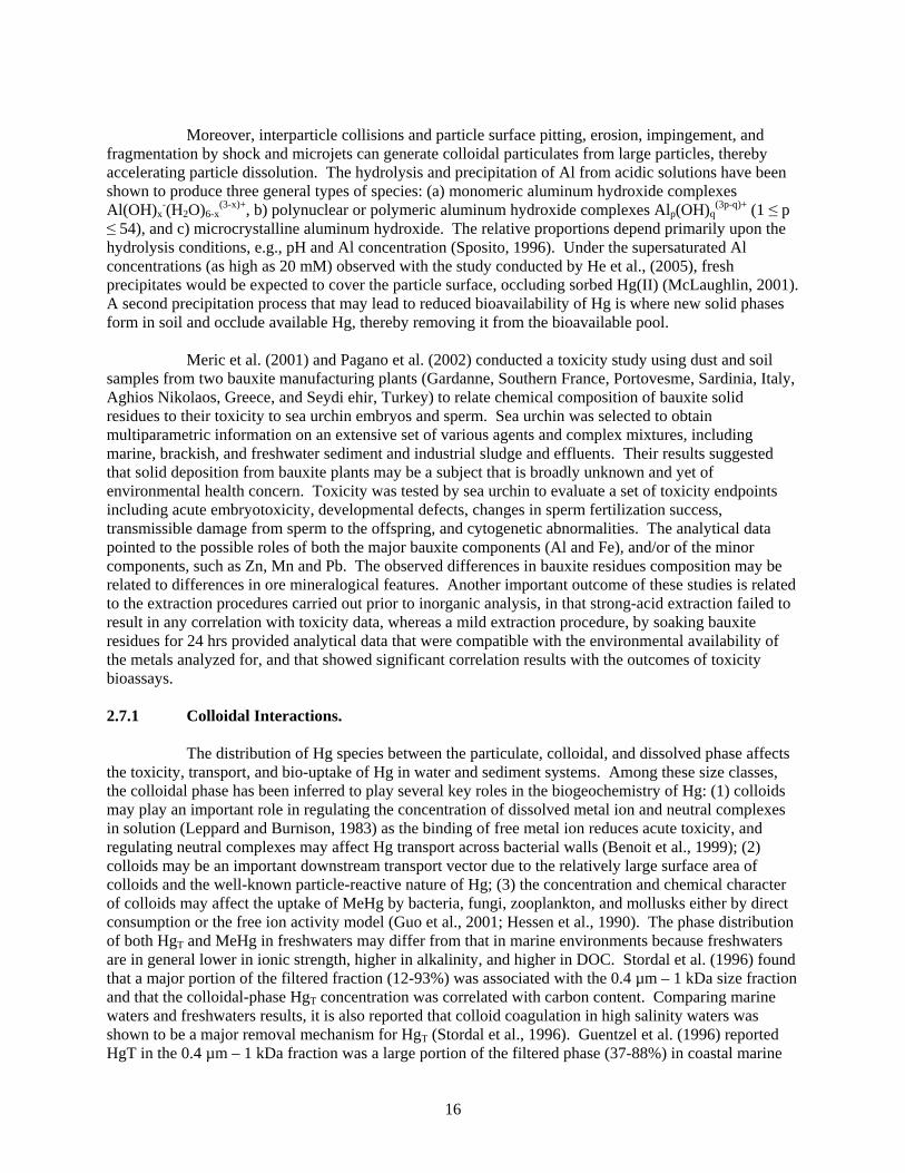
Diffusion and Advection (modified from Morel et al., 1998) 2.7 Interactions with Aluminosilicates Numerous studies have been conducted to examine Hg(II) sorption and release (desorption) from natural and synthetic particles, including clays (Sarkar et al., 2000), soils (Yin et al., 1997), sulfides (Ehrhardt et al., 2000), and (hydr)oxides (Sarkar et al., 2000). Complexation and adsorption of the precursor, Hg(II), by ligands and sediments may inhibit the production of methylmercury (Stein et al., 1996). The treatment and removal of Hg from sediments are necessary for control of methylation and bioaccumulation. As discrete particles and/or as coatings on other mineral surfaces in natural systems, especially in well-weathered soil and sediments with low natural organic matter, crystalline and amorphous alumina play significant roles (Sposito, 1996; Kasprzyk-Hordern 2004). Because of their chemical properties and physical structure, aluminum(hydr)-oxides are efficient sinks for many contaminants including cations of Pb, Zn, Cd, Sr, and Hg (Coston et al., 1995; Sarkar et al., 2000). In addition to Hg speciation, surface characteristics of aluminosilicates (surface area, porosity, pore size distribution, and PZC) can have a significant impact on the fate of these contaminants (Kasprzyk-Hordern, 2004). However, desorption of heavy metals from sediments and aluminosilicates can be much slower and/or nonreversible (Yin et al., 1997; Gao et al., 2003), which may lead to significant challenge due to longer time needed for the cleanup (He et al., 2005). Moreover, an oxidative environment via cavitation bubbles can be generated by use of sonic waves or biogenic gas cause mobilization of in-place sediment contaminants by gas ebullition.

16

Moreover, interparticle collisions and particle surface pitting, erosion, impingement, and fragmentation by shock and microjets can generate colloidal particulates from large particles, thereby accelerating particle dissolution. The hydrolysis and precipitation of Al from acidic solutions have been shown to produce three general types of species: (a) monomeric aluminum hydroxide complexes Al(OH)x

-(H2O)6-x(3-x)+, b) polynuclear or polymeric aluminum hydroxide complexes Alp(OH)q

(3p-q)+ (1 ≤ p ≤ 54), and c) microcrystalline aluminum hydroxide. The relative proportions depend primarily upon the hydrolysis conditions, e.g., pH and Al concentration (Sposito, 1996). Under the supersaturated Al concentrations (as high as 20 mM) observed with the study conducted by He et al., (2005), fresh precipitates would be expected to cover the particle surface, occluding sorbed Hg(II) (McLaughlin, 2001). A second precipitation process that may lead to reduced bioavailability of Hg is where new solid phases form in soil and occlude available Hg, thereby removing it from the bioavailable pool. Meric et al. (2001) and Pagano et al. (2002) conducted a toxicity study using dust and soil samples from two bauxite manufacturing plants (Gardanne, Southern France, Portovesme, Sardinia, Italy, Aghios Nikolaos, Greece, and Seydi ehir, Turkey) to relate chemical composition of bauxite solid residues to their toxicity to sea urchin embryos and sperm. Sea urchin was selected to obtain multiparametric information on an extensive set of various agents and complex mixtures, including marine, brackish, and freshwater sediment and industrial sludge and effluents. Their results suggested that solid deposition from bauxite plants may be a subject that is broadly unknown and yet of environmental health concern. Toxicity was tested by sea urchin to evaluate a set of toxicity endpoints including acute embryotoxicity, developmental defects, changes in sperm fertilization success, transmissible damage from sperm to the offspring, and cytogenetic abnormalities. The analytical data pointed to the possible roles of both the major bauxite components (Al and Fe), and/or of the minor components, such as Zn, Mn and Pb. The observed differences in bauxite residues composition may be related to differences in ore mineralogical features. Another important outcome of these studies is related to the extraction procedures carried out prior to inorganic analysis, in that strong-acid extraction failed to result in any correlation with toxicity data, whereas a mild extraction procedure, by soaking bauxite residues for 24 hrs provided analytical data that were compatible with the environmental availability of the metals analyzed for, and that showed significant correlation results with the outcomes of toxicity bioassays. 2.7.1 Colloidal Interactions. The distribution of Hg species between the particulate, colloidal, and dissolved phase affects the toxicity, transport, and bio-uptake of Hg in water and sediment systems. Among these size classes, the colloidal phase has been inferred to play several key roles in the biogeochemistry of Hg: (1) colloids may play an important role in regulating the concentration of dissolved metal ion and neutral complexes in solution (Leppard and Burnison, 1983) as the binding of free metal ion reduces acute toxicity, and regulating neutral complexes may affect Hg transport across bacterial walls (Benoit et al., 1999); (2) colloids may be an important downstream transport vector due to the relatively large surface area of colloids and the well-known particle-reactive nature of Hg; (3) the concentration and chemical character of colloids may affect the uptake of MeHg by bacteria, fungi, zooplankton, and mollusks either by direct consumption or the free ion activity model (Guo et al., 2001; Hessen et al., 1990). The phase distribution of both HgT and MeHg in freshwaters may differ from that in marine environments because freshwaters are in general lower in ionic strength, higher in alkalinity, and higher in DOC. Stordal et al. (1996) found that a major portion of the filtered fraction (12-93%) was associated with the 0.4 µm – 1 kDa size fraction and that the colloidal-phase HgT concentration was correlated with carbon content. Comparing marine waters and freshwaters results, it is also reported that colloid coagulation in high salinity waters was shown to be a major removal mechanism for HgT (Stordal et al., 1996). Guentzel et al. (1996) reported HgT in the 0.4 µm – 1 kDa fraction was a large portion of the filtered phase (37-88%) in coastal marine

17

water in the Ochlockonee River Estuary, Florida. They presented evidence that thiol functional groups associated with organic carbon were important in the partitioning of HgT in the colloidal phase. Their study also reported the first colloidal-phase MeHg concentrations in marine environments. Babiarz et al. (2001) studied partitioning of HgT and MeHg in 15 freshwater systems located in the upper Midwest (Minnesota, Michigan, and Wisconsin) and the Southern United States (Georgia and Florida). Though they reported that correlation between HgT and organic carbon in the colloidal phases was not statistically significant (r2 ≤ 0.14; p ≥ 0.07), MeHg in the colloidal phase and dissolved phase were correlated with the concentration of organic carbon as:

MeHgC = 0.15 × OCC + 0.0018 (r2 = 0.54, p < 0.01) MeHgD = 0.006 × OCD + 0.0458 (r2 = 0.23, p = 0.02) where, MeHg concentrations in colloidal phase and dissolved organic carbon phase are indicated as MeHgC and MeHgD, respectively).

2.7.2 Effect of Conductivity. A negative correlation between the rate of methylmercury formation and conductivity (salinity) in estuarine sediments has been reported (NOAA, 1996). The rate of MeHg formation is lower in more saline environment because the bicarbonate component of seawater slows methylation of Hg [II] under both aerobic and anaerobic conditions (Compeau and Bartha 1983). The release of reactive Hg [II] and Hg0 is slowed when chloride ions bind to mercury, thereby inhibiting methylmercury formation (Craig and Moreton 1985). Salinity also affects methylation due to the high pore-water sulfide concentrations as a result of rapid sulfate reduction in saline water compared to sulfate-limited freshwater environments (Gilmour et al. 1992). Gilmour and Henry (1991) reported that the percentage of total mercury that is methylmercury is higher in freshwater sediments (up to 37%) and water (up to 25% in aerobic water and 58% in anoxic bottom water) than in estuarine and marine water (<5%) and associated sediments (<5%). Dissolved reactive mercury (inorganic species) forms the majority of the total mercury in open oceans (Bloom and Crecilius 1983; Gill and Fitzgerald 1987). The study conducted by Babiarz et al. (2001) did not show strong trends in Hg concentration (ng g-1) with suspended particulate matter, conductivity, organic carbon in the <0.4 µm fraction, pH, or percent organic character, but MeHg concentration (ng g-1) was correlated with conductivity (µS cm-1) of the riverine water as:

[MeHg] = 14.6 + 0.0.295 – [conductivity] (r2 = 0.21, p = 0.03).

18

Section 3.0: PARTITION COEFFICIENTS OF MERCURY IN SEDIMENT Partitioning most likely plays a dominant role in the distribution of mercury species between the particulate, colloidal and dissolved phase controlling the toxicity, transport and bio-uptake of Hg (Stumm and Morgan, 1995). Inorganic Hg that is transported from soils and sediments to lakes is predominantly bound to dissolved or suspended organic matter (Mierle and Ingram, 1991; Hintelmann and Harris, 2004).

Figure 3-1. Sorption and Aging Processes Metals in Sediment A list of potential sorbents of mercury is summarized in Table 3.1.

19

Table 3-1. Sorption Capacities of Selected Sorbents

Sorbent Sorption Capacity Reference

Montmorillonite 296 – 346 mmol/kg

Cruz-Guzmán et al. (2003)

Humic acid 2700 – 2815 mmol/kg

Cruz-Guzmán et al. (2003)

Ferrihydrite 501 – 577 mmol/kg

Cruz-Guzmán et al. (2003)

Goethite (α-FeOOH) 0.39-0.42 µmol/m2

Kim et al. (2004a)

gamma-alumina (γ-Al2O3) 0.04-0.13 µmol/m2

Kim et al. (2004a)

Bayerite (β-Al(OH)3) 0.39-0.44 µmol/m2

Kim et al. (2004a)

Sorbent from Coriandrum sativum (coriander or Chinese parsley)

24-55 mg/g (Hg2+);

7-17 mg/g ( CH3Hg+)

Karunasagar et al. (2005)

Natural zeolites (clinoptilolite) 1.21 meq/g Chojnacki et al. (2004)

Activated carbon (clothe) 65 mg/g Babel and Kurniawan (2003)

Furfural-based carbon adsorbents

132-174 mg/g Budinova et al. (2003)

Yellow tuff (soft porous rock usually formed by compaction and cementation of volcanic ash or dust)

0.18 mg/g at 3000 µg/L

Natale et al. (2005)

Pozzolana (a type of slag that may be either natural—i.e., volcanic—or artificial, from a blast furnace)

0.8 mg/g at 1000 µg/L

Natale et al. (2005)

The sorption capacity of mercury on different natural adsorbents (illite, kaolinite, silica, and calcite) has been extensively studied under different experimental conditions (Gagnon and Fisher, 1997; De Diego et al., 2001). Other work has focused on determining partitioning constants of Hg(II) between water and sediments using natural particles (Stordal et al., 1996; Turner et al., 2001) or directly from field studies (Leermakers et al., 1995). Addition of Fe(II) ions in the presence of phlogopite (yellow to dark brown mica, general chemical formula KMg3[Si3Al]O10[F,OH]2) particles can enhance the reduction of Hg(II) (Charlet et al., 2002). The distribution coefficients kd obtained from sediment samples (log kd ranges from 4.5 to 6) greatly differ from one substrate to another, most likely due to the nature and abundance of respective binding sites. Nevertheless, the magnitude of log kd exemplifies the strong affinity of Hg(II) and MeHg to sediment and suspended particles. The kd values for Hg2+ and MeHg are comparable, but usually slightly lower for MeHg. Generally, the presence of organic matter enhances the sorption of Hg(II) to mineral surfaces (Gagnon and Fisher, 1997; Turner et al., 2001). Some studies investigated the partitioning between water and living biota, such as freshwater alga (Miles et al., 2001), bacteria (Hintelmann et al., 1993), periphyton (Cleckner et al., 1999) and phytoplankton (Watras et al.,

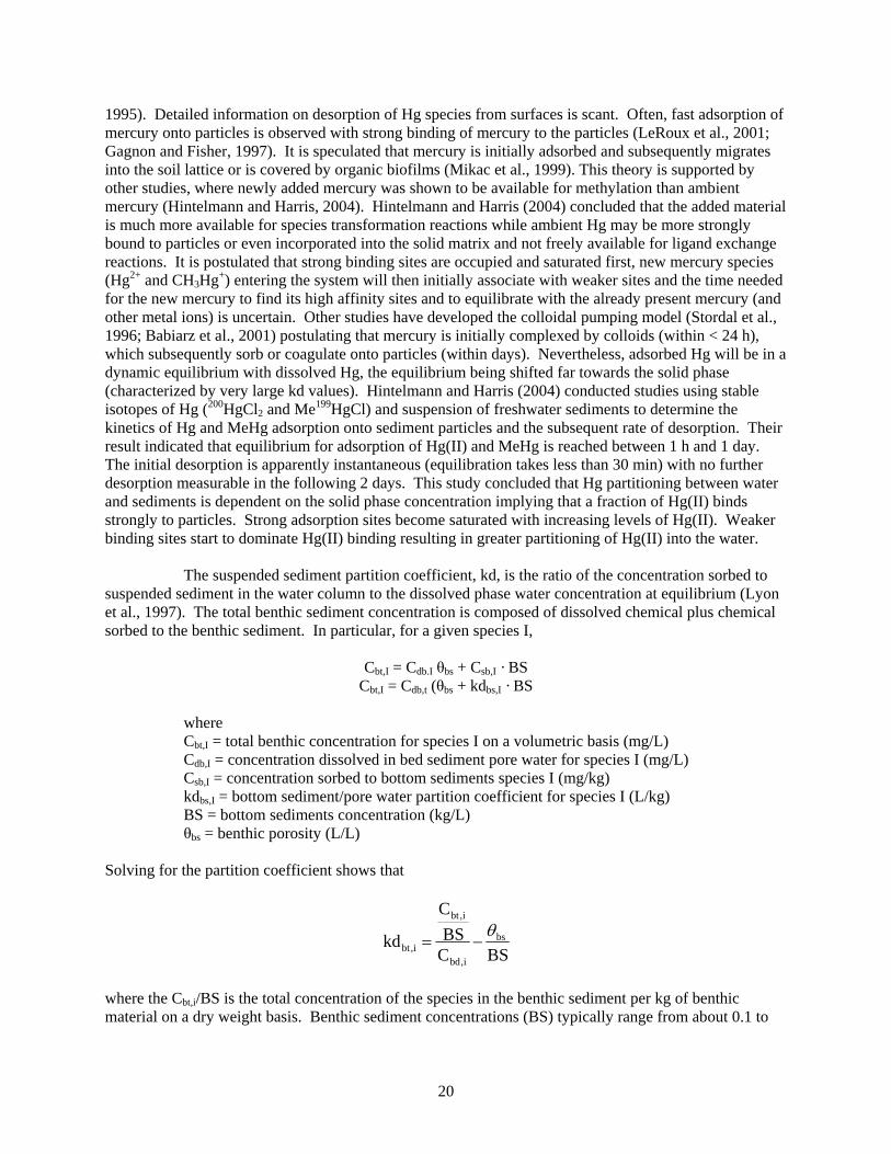
20

1995). Detailed information on desorption of Hg species from surfaces is scant. Often, fast adsorption of mercury onto particles is observed with strong binding of mercury to the particles (LeRoux et al., 2001; Gagnon and Fisher, 1997). It is speculated that mercury is initially adsorbed and subsequently migrates into the soil lattice or is covered by organic biofilms (Mikac et al., 1999). This theory is supported by other studies, where newly added mercury was shown to be available for methylation than ambient mercury (Hintelmann and Harris, 2004). Hintelmann and Harris (2004) concluded that the added material is much more available for species transformation reactions while ambient Hg may be more strongly bound to particles or even incorporated into the solid matrix and not freely available for ligand exchange reactions. It is postulated that strong binding sites are occupied and saturated first, new mercury species (Hg2+ and CH3Hg+) entering the system will then initially associate with weaker sites and the time needed for the new mercury to find its high affinity sites and to equilibrate with the already present mercury (and other metal ions) is uncertain. Other studies have developed the colloidal pumping model (Stordal et al., 1996; Babiarz et al., 2001) postulating that mercury is initially complexed by colloids (within < 24 h), which subsequently sorb or coagulate onto particles (within days). Nevertheless, adsorbed Hg will be in a dynamic equilibrium with dissolved Hg, the equilibrium being shifted far towards the solid phase (characterized by very large kd values). Hintelmann and Harris (2004) conducted studies using stable isotopes of Hg (200HgCl2 and Me199HgCl) and suspension of freshwater sediments to determine the kinetics of Hg and MeHg adsorption onto sediment particles and the subsequent rate of desorption. Their result indicated that equilibrium for adsorption of Hg(II) and MeHg is reached between 1 h and 1 day. The initial desorption is apparently instantaneous (equilibration takes less than 30 min) with no further desorption measurable in the following 2 days. This study concluded that Hg partitioning between water and sediments is dependent on the solid phase concentration implying that a fraction of Hg(II) binds strongly to particles. Strong adsorption sites become saturated with increasing levels of Hg(II). Weaker binding sites start to dominate Hg(II) binding resulting in greater partitioning of Hg(II) into the water. The suspended sediment partition coefficient, kd, is the ratio of the concentration sorbed to suspended sediment in the water column to the dissolved phase water concentration at equilibrium (Lyon et al., 1997). The total benthic sediment concentration is composed of dissolved chemical plus chemical sorbed to the benthic sediment. In particular, for a given species I,

Cbt,I = Cdb.I θbs + Csb,I · BS Cbt,I = Cdb,t (θbs + kdbs,I · BS

where Cbt,I = total benthic concentration for species I on a volumetric basis (mg/L) Cdb,I = concentration dissolved in bed sediment pore water for species I (mg/L) Csb,I = concentration sorbed to bottom sediments species I (mg/kg) kdbs,I = bottom sediment/pore water partition coefficient for species I (L/kg) BS = bottom sediments concentration (kg/L) θbs = benthic porosity (L/L)

Solving for the partition coefficient shows that

BSCBSC

kd bs

i,bd

i,bt

i,btθ

−=

where the Cbt,i/BS is the total concentration of the species in the benthic sediment per kg of benthic material on a dry weight basis. Benthic sediment concentrations (BS) typically range from about 0.1 to

21

1.5 kg/L, and benthic porosity typically ranges between 0.4 and 0.99. Thus, the term θbs/BS is at most about 10 L/kg, and can be ignored if the other term defining the partition coefficient is large. A positive control, consisting of the species I (say, Hg2+-spiked) solution without any sediment, and a negative control, consisting of surface water and sediment but without added Hg2+, should be carried out through the testing. Results from the positive control expected to indicate whether sorption to the labware [glass reported not to sorb measurable amount of Hg2+ (Kaplan et al., 2002)], Hg precipitation, or Hg volatilization occurring or not. Results from the negative control expected to indicate whether any amount of Hg could be introduced into the system from the uncontaminated sediment and surface water. Finally, the degree to which Hg could be filtered from the spiked solutions (the positive controls) should be determined. It can be quantified as a filtration ratio (FR):

⎟⎟⎠

⎞⎜⎜⎝

⎛=

unfiltered

filtered

HgHgFR

where Hgfiltered and Hgunfiltered are the Hg concentrations in the spiked solution after and before, respectively, passing through a filter. The filtration ratio can be included to provide another index as to whether precipitation of the added Hg2+ occurred during the equilibration period. If the filtration ratio of the spiked solution is near unity, it indicates that little of the Hg2+ in the spike solution is filterable. As the Hg bioavailability and propensity to sorb to sediments is largely controlled by Hg-speciation and its oxidation state, the ORP, pH, and temperature need to be measured in the field following the procedure of Patrick et al. (1996) or equivalent. Briefly, sediment samples can be collected by scraping away the litter layer from the ground and scooping 20-cm3 of the surface mineral layer into a disposable plastic cup. Approximately 20-cm3 of distilled-deionized water needs to be added to the sediment. The suspensions should be stirred and allowed to equilibrate for 30-min. Eh, pH, and temperature need to be measured in the sediment slurry. Appropriate calibration of the electrodes should be conducted prior to the measurement. ORP results should be converted to Standard Hydrogen Electrode (SHE), taking into consideration field temperature at the time of the Eh measurement. In the literature, there are limited measured data under realistic conditions available. For divalent mercury (Hg[II]), Moore and Ramamodomy (1984) reported kd as a range of 1380-188,000 L/kg, Glass et al. (1990) reported a value of 118,000 L/kg, and Robinson and Shuman (1989) reported a range of 86,800-113,000 L/kg. For methylmercury, Bloom et al. (1989) indicated that regardless of pH, for over three orders of magnitude, the log kd for seston (suspended matter) was in the range of 5.5 to 6.0, which corresponds to a range from 316,000 to 1,000,000 L/kg. Babiarz et al. (2001) results show that log kd for HgT ranged from 3.9 to 6.4 with a median of 5.0 and for MeHg ranged from 3.7 to 6.3, again with a median of 5.0. Lyon et al. (1997) calculated the benthic sediment partition coefficients for Hg(II) and MeHg based on the data available in the literature (see Table 3-2). It should be noted that partitioning coefficients for mercury species are dependent on considerable site-specific variability, and hence judgment should always be utilized as appropriate. The loads of MeHg from surface runoff/erosion are a significant contribution to the MeHg stored in water bodies. MeHg concentrations in fish in Swedish lakes were explained in terms of the fluxes MeHg into the water bodies from the measured direct deposition rates and runoff/erosion loads from the watershed. However, for some lakes with minimal Hg input from the watershed suggested that bioavailable MeHg was created within the lake itself. Lyon et al. (1997) concluded that for lakes with appreciable input from the watershed, MeHg in the water body could be due a combination of in-lake net methylation and input from deposition and/or runoff/erosion. Many processes influence the fate of contaminants in bottom sediments. Contaminants can be transported into the overlying water column by advective and diffusive mechanisms. Mixing and

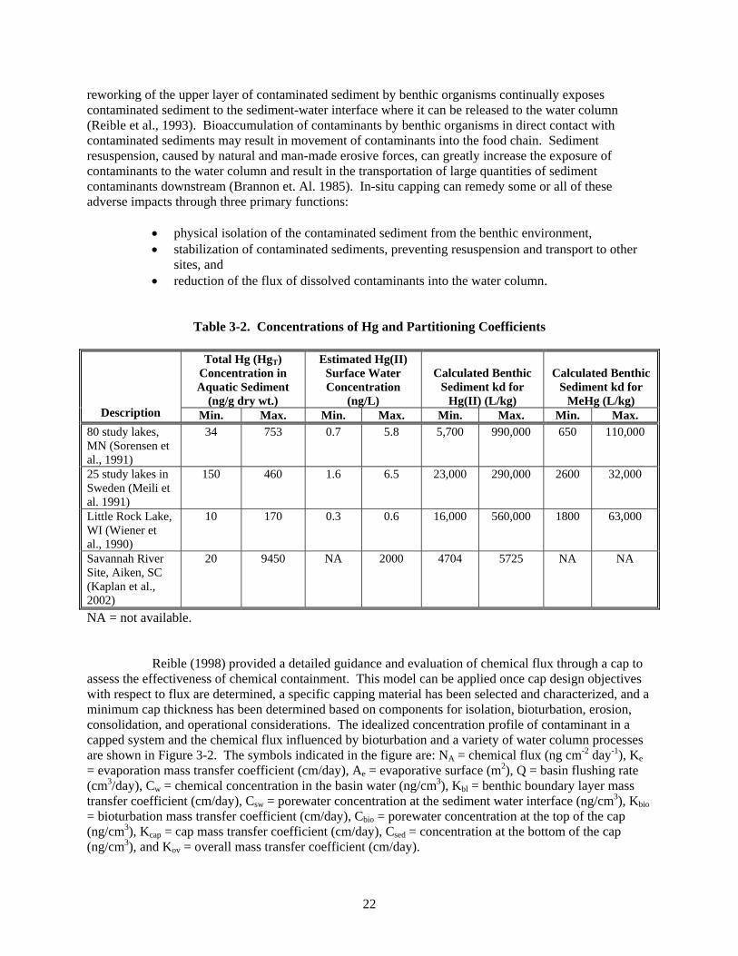
22

reworking of the upper layer of contaminated sediment by benthic organisms continually exposes contaminated sediment to the sediment-water interface where it can be released to the water column (Reible et al., 1993). Bioaccumulation of contaminants by benthic organisms in direct contact with contaminated sediments may result in movement of contaminants into the food chain. Sediment resuspension, caused by natural and man-made erosive forces, can greatly increase the exposure of contaminants to the water column and result in the transportation of large quantities of sediment contaminants downstream (Brannon et. Al. 1985). In-situ capping can remedy some or all of these adverse impacts through three primary functions:

• physical isolation of the contaminated sediment from the benthic environment, • stabilization of contaminated sediments, preventing resuspension and transport to other

sites, and • reduction of the flux of dissolved contaminants into the water column.

Table 3-2. Concentrations of Hg and Partitioning Coefficients

Total Hg (HgT) Concentration in Aquatic Sediment

(ng/g dry wt.)

Estimated Hg(II) Surface Water Concentration

(ng/L)

Calculated Benthic Sediment kd for

Hg(II) (L/kg)

Calculated Benthic Sediment kd for

MeHg (L/kg) Description Min. Max. Min. Max. Min. Max. Min. Max.

80 study lakes, MN (Sorensen et al., 1991)

34 753 0.7 5.8 5,700 990,000 650 110,000

25 study lakes in Sweden (Meili et al. 1991)

150 460 1.6 6.5 23,000 290,000 2600 32,000

Little Rock Lake, WI (Wiener et al., 1990)

10 170 0.3 0.6 16,000 560,000 1800 63,000

Savannah River Site, Aiken, SC (Kaplan et al., 2002)

20 9450 NA 2000 4704 5725 NA NA

NA = not available. Reible (1998) provided a detailed guidance and evaluation of chemical flux through a cap to assess the effectiveness of chemical containment. This model can be applied once cap design objectives with respect to flux are determined, a specific capping material has been selected and characterized, and a minimum cap thickness has been determined based on components for isolation, bioturbation, erosion, consolidation, and operational considerations. The idealized concentration profile of contaminant in a capped system and the chemical flux influenced by bioturbation and a variety of water column processes are shown in Figure 3-2. The symbols indicated in the figure are: NA = chemical flux (ng cm-2 day-1), Ke = evaporation mass transfer coefficient (cm/day), Ae = evaporative surface (m2), Q = basin flushing rate (cm3/day), Cw = chemical concentration in the basin water (ng/cm3), Kbl = benthic boundary layer mass transfer coefficient (cm/day), Csw = porewater concentration at the sediment water interface (ng/cm3), Kbio = bioturbation mass transfer coefficient (cm/day), Cbio = porewater concentration at the top of the cap (ng/cm3), Kcap = cap mass transfer coefficient (cm/day), Csed = concentration at the bottom of the cap (ng/cm3), and Kov = overall mass transfer coefficient (cm/day).

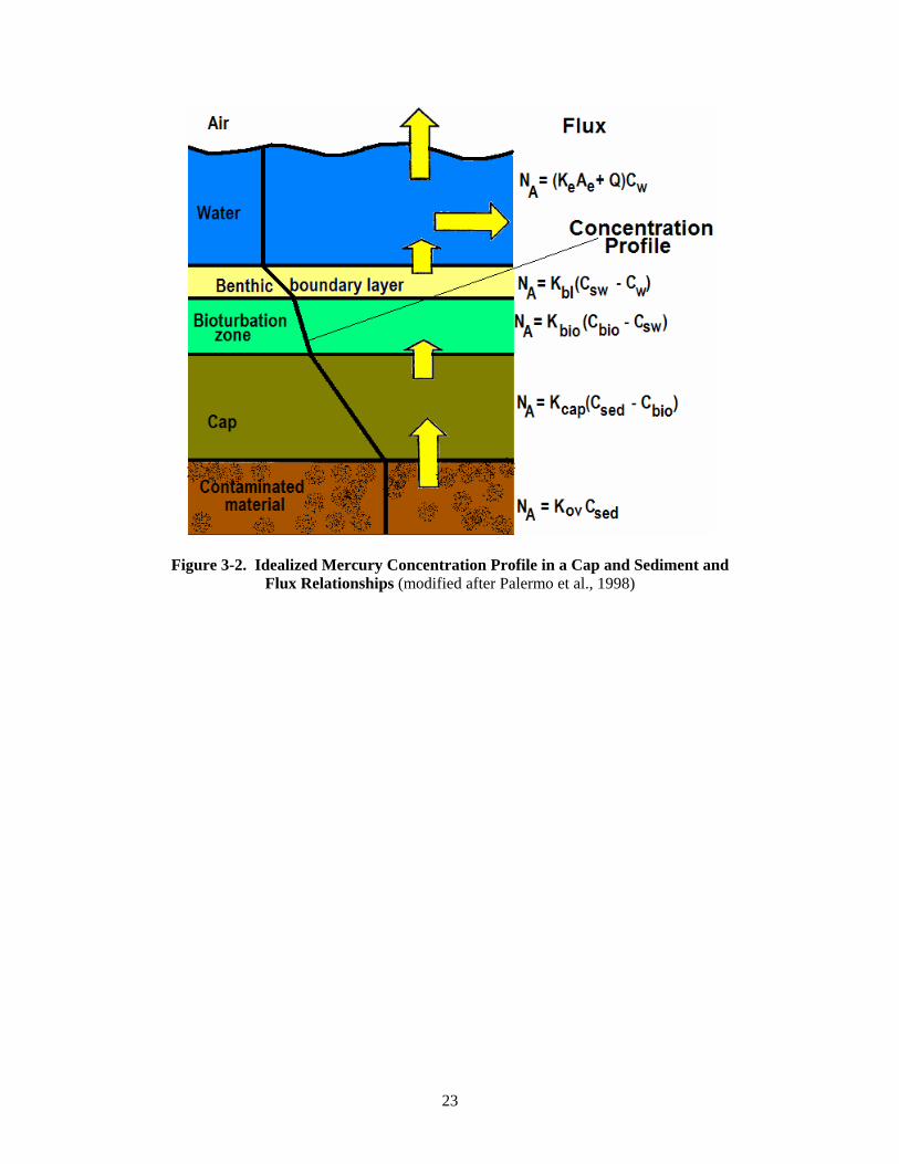
23

Figure 3-2. Idealized Mercury Concentration Profile in a Cap and Sediment and Flux Relationships (modified after Palermo et al., 1998)

24

Section 4.0: MATHEMATICAL MODELS Mathematical models can help us understand the important processes and interactions that affect the water quality. These models can be used in making decisions regarding pollution control strategies by evaluating their effectiveness on water quality improvement and performing cost-benefit analysis. Models are extensively used by water resources planner, water quality managers, remedial project managers, environmental engineers and scientists to evaluate effectiveness of various control strategies. The success in utilization of models in various environmental applications has resulted in wide acceptance of models as an objective evaluation tool and as a result they are often given higher credibility than what they actually deserve. Models are only approximate representations of the complex natural processes and due to time and budget constraints involve many assumptions made by the model developer who defines the relationship between various processes, and the model programmer who carries the model into computer platforms. Certain simplification considered for one application might not be valid for other application due to the uniqueness of a problem and counter-intuitive results may be produced (AWWA, 2001). Modeling also involves a profusion of uncertainty. Macintosh et al. (1994) defined two types of uncertainty: (a) knowledge uncertainty, which is associated with measurement errors and inability of the model to accurately represent the physical, chemical, and biological processes; and (b) stochastic uncertainty, which arises from the random nature of natural systems like rainfall, natural heterogeneity of sediment. Any modeling application comprises both types of uncertainties implying that modeling cannot be deemed as representing the absolute truth (Kalin and Hantush, 2003). Based on functionality, suspended solids and sediments (SSAS), and nutrients water quality models can be broadly categorized into three groups: (a) loading models, which simulate field scale hydrologic processes and determine the generation and transport of SSAS and nutrients from source in the upper lands to the receiving water; (b) receiving water models, which includes hydrodynamic models (hydraulics of water quality models for transport, deposition, circulation, and stratification processes), and water quality models to simulate the movement of SSAS in the water column and determine the fate and transport of contaminants, nutrients; and (c) eutrophication/ecological models, which relate to biomass production, sediment flux, growth in the water body to contaminant and/or nutrient loading, and photosynthesis. The relationship between these models is shown in Figure 4-1.

Figure 4-1. Mathematical Model Framework and Relationship Between Various Models

SEDIMENT TRANSPORT MODEL

Sediment Resuspension and Deposition Fluxes

CONTAMINANT FATE MODEL

Water Column and Sediment Concentrations

Current Velocity

Current Velocity, Bottom Shear Stress,

Stage Height

BANK EROSION MODEL

Sediment and Contaminant Loads

EUTROPHICATION/ ECOLOGICAL MODEL

River/Streams, Lakes/Reservoirs,

Estuaries/Bays

RECEIVING WATER MODEL

LOADING MODEL

Generation and Transport of SSAS

HYDRODYNAMIC MODEL

25

Utilities of mathematical model are:

• Constrain, synthesize, and interpret data, • Quantify effects of different transport processes, • Make quantitative predictions, • Develop insights about processes that affect sediment stability.

The limitations of the mathematical models are:

• Data collection to support model development and calibration, • Level of uncertainty in results may be unacceptable to stakeholders and decision-makers.

Uncertainty bounds on predictions are the key issues regarding model reliability and utility at a particular site. However, sediment stability studies conducted at a variety of sites demonstrate that useful models can be developed provided that sufficient site-specific data are available, and an experienced modeling team conducts the study (Ziegler, 2005). Seven principles need to be considered in developing and using numerical models at sediment sites (EPA, 2005).

(1) Develop and refine a conceptual site model that identifies the key areas of uncertainty where modeling information may be needed.

(2) Consider site complexity before deciding if a mathematical model is necessary.

(3) Determine what model output data are needed to facilitate decision-making.

(4) Consider modeling results in conjunction with empirical data to inform site decision-making.

(5) Conduct a complete modeling study. If an intermediate or advanced level model is used in decision-making, the following components should be included in every modeling effort: • Model verification. Evaluating the model theory, consistency of the computer code

with model theory, and evaluation of the code for integrity in the calculations. • Model calibration. Using site-specific information from a historical period of time to

adjust model parameters in the governing equations to obtain an optimal agreement between a measured data set and model calculations for the simulated state variables.

• Model validation. Demonstrating that the calibrated model accurately reproduces known conditions over a different period of time with the physical parameters and forcing functions changed to reflect the conditions during the new simulation period.

• Sensitivity analysis. This process consists of varying each of the input parameters by a fixed percent (while holding the other parameters constant) to determine how the predictions vary. The resulting variations in the state variables are a measure of the sensitivity of the model predictions to the parameter whose value was varied.

• Uncertainty analysis. This process consists of propagating the relative error in each parameter (that was varied during the sensitivity analysis) to determine the resulting error in the model predictions.

(6) Understand and explain model uncertainty

26

(7) Learn from modeling efforts and be prepared to refine a model based upon post-remedy evaluation.

Description, advantages and disadvantages of five sediment transport models are indicated in Table 4-1 (Jones and Roberts, 2005).

Table 4-1. Comparison of Sediment Transport Models

Sediment Transport

Model Description Advantages Disadvantages SED2D Cohesive and non-

cohesive sediment transport model.

Integrated with hydrodynamics package in a user friendly environment.

Only provides for a single grain size per simulation. Generally not applicable for contaminant transport applications.

EFDC Cohesive and non-cohesive sediment transport model.

Integrated with 3-D hydrodynamics. It includes multiple size classes, bed load transport, and bed armoring.

Based on dated cohesive sediment dynamics. Difficult to incorporate site specific sediment stability measurements without modification.

SEDZL Cohesive and non-cohesive sediment transport model.

Integrated with 2D hydrodynamics model. Based on site specific sediment data (Shaker). This model has been applied at a number of contaminated sediment sites.

Limited to 2D hydrodynamics. Based on surficial sediment stability measurements.

ECOM-SED Cohesive and non-cohesive sediment transport model.

Utilizes SEDZL model coupled to 3D hydrodynamics model.

Based on surficial sediment stability measurements. Hydroqual, Inc. proprietary model. However, no fee for use.

SEDZL-J Cohesive and non-cohesive sediment transport model.

Integrated with SEDZL 2D hydrodynamics model. Based on site specific sediment stability data with depth into sediments (Sedflume).

Currently limited to 2D hydrodynamics. This model has not been widely applied.

4.1 Models to Simulate Hg Transport and Transformation Simulation of mercury transport and transformation in aquatic systems is complex, involving hydrodynamic and sediment processes and mercury transport and transformation processes. Considerable site-specific data are needed to calibrate and validate mercury transport and transformation models. Because of limitations in analysis accuracy, mercury data reported before the 1980s should be reviewed with caution (Braga et al., 2000). Based on the type of aquatic systems, Wang et al. (2004) conducted literature review on mercury transport and transformation models. They categorized the models in three types of systems: (1) river, (2) lake, and (3) coastal. Table 4-2 lists some existing Hg transport and transformation models.

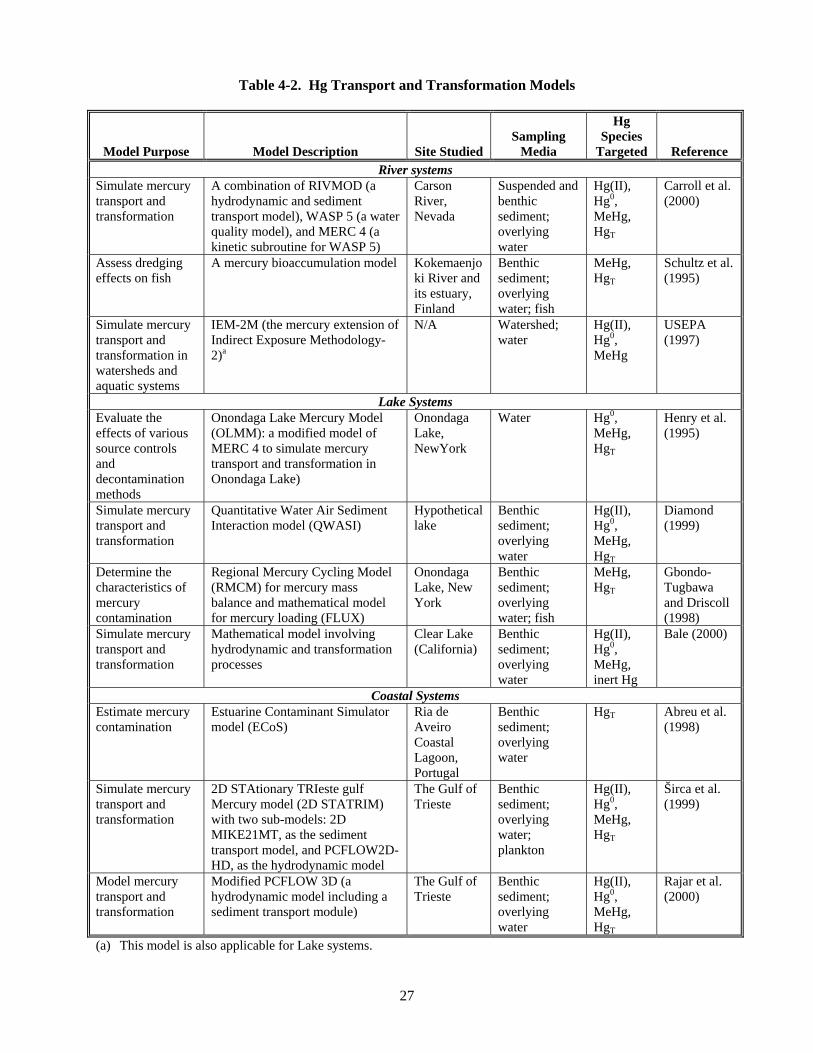
27

Table 4-2. Hg Transport and Transformation Models

Model Purpose Model Description Site Studied Sampling

Media

Hg Species

Targeted Reference River systems

Simulate mercury transport and transformation

A combination of RIVMOD (a hydrodynamic and sediment transport model), WASP 5 (a water quality model), and MERC 4 (a kinetic subroutine for WASP 5)

Carson River, Nevada

Suspended and benthic sediment; overlying water

Hg(II), Hg0, MeHg, HgT

Carroll et al. (2000)

Assess dredging effects on fish

A mercury bioaccumulation model Kokemaenjoki River and its estuary, Finland

Benthic sediment; overlying water; fish

MeHg, HgT

Schultz et al. (1995)

Simulate mercury transport and transformation in watersheds and aquatic systems

IEM-2M (the mercury extension of Indirect Exposure Methodology-2)a

N/A Watershed; water

Hg(II), Hg0, MeHg

USEPA (1997)

Lake Systems Evaluate the effects of various source controls and decontamination methods

Onondaga Lake Mercury Model (OLMM): a modified model of MERC 4 to simulate mercury transport and transformation in Onondaga Lake)

Onondaga Lake, NewYork

Water Hg0, MeHg, HgT

Henry et al. (1995)

Simulate mercury transport and transformation

Quantitative Water Air Sediment Interaction model (QWASI)

Hypothetical lake

Benthic sediment; overlying water

Hg(II), Hg0, MeHg, HgT

Diamond (1999)

Determine the characteristics of mercury contamination

Regional Mercury Cycling Model (RMCM) for mercury mass balance and mathematical model for mercury loading (FLUX)

Onondaga Lake, New York

Benthic sediment; overlying water; fish

MeHg, HgT

Gbondo-Tugbawa and Driscoll (1998)

Simulate mercury transport and transformation

Mathematical model involving hydrodynamic and transformation processes

Clear Lake (California)

Benthic sediment; overlying water

Hg(II), Hg0, MeHg, inert Hg

Bale (2000)

Coastal Systems Estimate mercury contamination

Estuarine Contaminant Simulator model (ECoS)

Ria de Aveiro Coastal Lagoon, Portugal

Benthic sediment; overlying water

HgT

Abreu et al. (1998)

Simulate mercury transport and transformation

2D STAtionary TRIeste gulf Mercury model (2D STATRIM) with two sub-models: 2D MIKE21MT, as the sediment transport model, and PCFLOW2D-HD, as the hydrodynamic model

The Gulf of Trieste

Benthic sediment; overlying water; plankton

Hg(II), Hg0, MeHg, HgT

Širca et al. (1999)

Model mercury transport and transformation

Modified PCFLOW 3D (a hydrodynamic model including a sediment transport module)

The Gulf of Trieste

Benthic sediment; overlying water

Hg(II), Hg0, MeHg, HgT

Rajar et al. (2000)

(a) This model is also applicable for Lake systems.

28

Limited numbers of mercury transport and transformation models are available in the literature. Only a few models link the modeling tool with contamination remediation and predict the remedial results in benthic sediment and overlying water. While many of the fate and transport processes vary significantly in importance from site to site, Sediment Management Work Group (1999) recognized that it is possible to rank the potential importance of each mechanism using characteristic times. Characteristic times are order of magnitude estimates of time required to remove contaminate of concern (COCs) from an initially uniformly contaminated layer of height (H) by each of the various transport mechanisms. In most cases, the characteristic times represent times required to achieve 37% of the initial sediment bed concentration or 63% percent recovery. In the case of advective processes, the characteristic times represent complete removal times. Table 4-3 summarizes the relationships comparing the characteristic recovery times of contaminated sediment by each of the processes. Processes that exhibit a shorter characteristic time are likely to be the most important transport processes.

Table 4-3. Summary of Characteristic Times of Sediment Fate and Transport Processes

Process Characteristic Time

Relationship Typical Range of Key

Parameter Values Illustrative Value of Characteristic Time1

Diffusion

eff

f2

2 DRH4

πτ =

Rf > 1,000 (hydrophobic organics); Deff ~ 10-6 cm2/s

1,280 years

Advection

ντ fHR=

Groundwater velocity, v, widely variable

100 years

Sediment erosion

UH

ero =τ Bed erosion rate, U, widely variable

10 years

Bioturbation

bio

2

2 DH4

πτ =

0.3 cm2/yr<Dbio<30 cm2/yr

13 years

Reaction

rxnfate k

1=τ

Reaction rate, krxn, widely variable

100 years

(1) It was assumed a 10 cm thick surficial layer contaminated with a hydrophobic organic with an effective retardation factor of 1,000. A groundwater velocity of 1 m/yr, a bed erosion rate of 1 cm/yr, an effective bioturbation diffusion coefficient of 3 cm2/yr and a reaction rate of 0.01 yr-1 were assumed.

The U.S. EPA is currently exploring the Free Ion Activity (FIA) paradigm for potential use as a more accurate predictor of ionic toxicant bioavailability in natural water. An implicit requirement of the FIA model is a fundamental understanding of the aqueous speciation behavior of those ionic species of interest. For example, both MeHg can exist as a suite of species in natural waters: CH3Hg+, CH3HgOH, CH3HgCl, CH3HgS-,and CH3HgSR (R is functional group of natural organic carbon and does not exist as a unique compound). Geochemical speciation models require both an innate database of reaction constants that enable one to model complex competitive geochemical speciation simulations and user input containing the total analytical concentrations of the reacting species of interest. Given the complexity of the various, simultaneous (and competing) equilibrium reactions governing the speciation of ionic species in aquatic systems, U.S. EPA has addressed a limitation found in earlier versions of

29

MINTEQA2 by extending the existing reaction constant database and enhancing capability for modeling the aqueous speciation behavior of MeHg in environmental aquatic systems (Loux, 2005). The speciation of mercury is an important consideration in any representation of mercury fate and transport. Depending upon its speciation, mercury may be either available or unavailable for biogeochemical reactions. Based upon a series of chemical procedures, four predominant species of mercury within an aquatic system has been identified into which the aquatic mercury pool may reasonably be subdivided for modeling (Meili, 1991; Hudson et al., 1994). These identifiable components of the aquatic mercury pool include:

•• Reactive mercury (Hg[II]) •• Monomethylmercury (MeHg) •• Elemental mercury (Hg0) •• Non-reactive mercury that is also biochemically unavailable (InertHg)

Bale (2000) described rates of transformation among the four fundamental mercury species to calculate the partitioning of mercury species between the dissolved and particulate-bound phases. The various physical and biochemical rate processes included for the mercury cycle were:

•• Atmospheric deposition •• Diffusive exchange with the atmosphere •• Biogeochemical transformation of mercury species •• Biouptake by aquatic species in the food chain •• Adsorption and desorption of mercury to particulates •• Diffusive exchange between the water column and sediment bed •• Deposition and resuspension of suspended sediment and bound mercury •• Burial of contaminated sediments

The model of mercury fate and transport developed by Bale (2000) was designed for incorporation into an advection-diffusion equation, and may be applied to aquatic systems with complex morphology and hydrodynamics. He demonstrated that this model, calibrated at three sites and validated at four sites within Clear Lake, CA, can reasonably simulate total Hg and MeHg as functions of sediment HgT. The model demonstrated that methylation of biochemically available HgT can be the principal source of MeHg in the lake. With only a small fraction of HgT available, the model was able to account for all MeHg in the lake at methylation rates that correspond well to those observed in other studies. The dominant cycling mechanism for Hg in the lake appears to be diffusion-dispersion upward from the sediment bed and a corresponding depositional load of nearly equal magnitude. The model indicated that the lake is experiencing a steady decline in Hg burden due in great part to burial of surficial sediments. Still, natural remediation of Clear Lake through burial is a slow process and may be expected to remove less than 2% of Clear Lake’s Hg burden each year. At such a remediation rate, Bale (2004) estimated that mercury concentrations in the lake would meet current water-quality criteria in a little over 200 years. 4.3 Water Quality Analysis Simulation Program to Simulate Hg Transport and

Speciation in Water column and Benthic Sediment Kim et al. (2004b) conducted a simulation of the fate of Hg in aquatic systems by modifying Water Quality Analysis Simulation Program (WASP) as part of a remedial investigation of Onondaga Lake, NY. Remediation strategies included were: dredging, capping and natural attenuation. Their model predictions for the water column generally agreed with the measured values reported in the literature for

30

Onondaga Lake. The authors estimated the remobilization of sediment based on cutterhead suction dredging process with a rate of 15 000 m3 of sediment per hour and sediments from the sediment–water interface up to 20 cm deep were removed during 20 working days with an estimated removed sediment volume of 2.4 × 106 /m3. The input parameters used for model simulations are shown in Table 4-4.

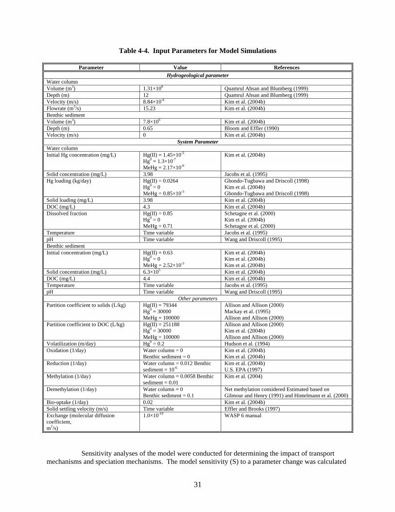
31

Table 4-4. Input Parameters for Model Simulations

Parameter Value References Hydrogeological parameter

Water column Volume (m3) 1.31×108 Quamrul Ahsan and Blumberg (1999) Depth (m) 12 Quamrul Ahsan and Blumberg (1999) Velocity (m/s) 8.84×10-4 Kim et al. (2004b) Flowrate (m3/s) 15.23 Kim et al. (2004b) Benthic sediment Volume (m3) 7.8×106 Kim et al. (2004b) Depth (m) 0.65 Bloom and Effler (1990) Velocity (m/s) 0 Kim et al. (2004b)

System Parameter Water column Initial Hg concentration (mg/L) Hg(II) = 1.45×10-5

Hg0 = 1.3×10-7 MeHg = 2.17×10-6

Kim et al. (2004b)

Solid concentration (mg/L) 3.98 Jacobs et al. (1995) Hg loading (kg/day) Hg(II) = 0.0264

Hg0 = 0 MeHg = 0.85×10-3

Gbondo-Tugbawa and Driscoll (1998) Kim et al. (2004b) Gbondo-Tugbawa and Driscoll (1998)

Solid loading (mg/L) 3.98 Kim et al. (2004b) DOC (mg/L) 4.3 Kim et al. (2004b) Dissolved fraction Hg(II) = 0.85

Hg0 = 0 MeHg = 0.71

Schetagne et al. (2000) Kim et al. (2004b) Schetagne et al. (2000)

Temperature Time variable Jacobs et al. (1995) pH Time variable Wang and Driscoll (1995) Benthic sediment Initial concentration (mg/L) Hg(II) = 0.63

Hg0 = 0 MeHg = 2.52×10-3

Kim et al. (2004b) Kim et al. (2004b) Kim et al. (2004b)

Solid concentration (mg/L) 6.3×105 Kim et al. (2004b) DOC (mg/L) 4.4 Kim et al. (2004b) Temperature Time variable Jacobs et al. (1995) pH Time variable Wang and Driscoll (1995)

Other parameters Partition coefficient to solids (L/kg)

Hg(II) = 79344 Hg0 = 30000 MeHg = 100000

Allison and Allison (2000) Mackay et al. (1995) Allison and Allison (2000)

Partition coefficient to DOC (L/kg) Hg(II) = 251188 Hg0 = 30000 MeHg = 100000

Allison and Allison (2000) Kim et al. (2004b) Allison and Allison (2000)

Volatilization (m/day) Hg0 = 0.2 Hudson et al. (1994) Oxidation (1/day) Water column = 0

Benthic sediment = 0 Kim et al. (2004b) Kim et al. (2004b)

Reduction (1/day) Water column = 0.012 Benthic sediment = 10-6

Kim et al. (2004b) U.S. EPA (1997)

Methylation (1/day) Water column = 0.0058 Benthic sediment = 0.01

Kim et al. (2004)

Demethylation (1/day) Water column = 0 Benthic sediment = 0.1

Net methylation considered Estimated based on Gilmour and Henry (1991) and Hintelmann et al. (2000)

Bio-uptake (1/day) 0.02 Kim et al. (2004b) Solid settling velocity (m/s) Time variable Effler and Brooks (1997) Exchange (molecular diffusion coefficient, m2/s)

1.0×10-10 WASP 6 manual

Sensitivity analyses of the model were conducted for determining the impact of transport mechanisms and speciation mechanisms. The model sensitivity (S) to a parameter change was calculated

32

as the relative change in the Hg concentration divided by the relative change in parameter value (U.S. EPA, 1997)

100

PPP

CCC

(%)S

B

B

B

B

×−

−

=

where CB is the calculated value of model output in the base simulation, C is the calculated value of model output after a change in parameter, PB is the model parameter value in the base simulation and P is the model parameter value in the sensitivity simulation. Kim et al. (2004b) analyzed their model based on following parameters:

• Biouptake, • Demethylation, • Methylation, • Reduction, • Volatilization, • Sorption, • Advection, • Settling • Diffusion

The simulation results concluded that advection, sorption and settling were important mechanisms of Hg transport in the water column. In the benthic sediment, settling of Hg from the water column was the most important input source of Hg. Both in the water column and the benthic sediment, reduction, methylation and demethylation were important mechanisms of Hg speciation. While authors assumed that Hg loading is steady, they reported that natural attenuation had no effect on the remediation of Hg-contaminated aquatic systems as compared with dredging and capping actions. Authors concluded that dredging and capping can be alternatives to remediation for Hg-contaminated aquatic systems. It was also recognized that this simulation might have uncertainties in the prediction of Hg cycling considering the complexity of Hg speciation and transport. 4.4 Sampling Design for Contaminant Distribution in Sediment A sampling design methodology for monitoring contaminant distribution in lake sediments was reported by Ben-Jemaa et al. (1995) using two optimization approaches: a minimization of the variance of estimation approach and a sampling cost minimization approach, allowing an economically efficient sampling design and a decision-making tool given the multi-objective nature of the problem. The concept of sampling network design is, however, widely used in the domain of groundwater monitoring and two main approaches have been identified - the hydrogeological approach and the statistical approach. Unlike the latter, the former is fully based on qualitative and quantitative hydrogeological information. The statistical approach has employed variance minimization and/or optimization methods. As the estimates of pollutant concentrations are very important inputs for hydrological models, a plausible sampling network provides accurate parameter estimates with a low variance of error estimation. The total monitoring cost is also an important factor in the sampling network design. To

33

increase monitoring efficiency, a network design yielding a low monitoring cost is preferred. However, there exists a trade off between the monitoring cost reduction and estimation variance minimization. Ben-Jemma et al. (1995) developed two optimization models: (a) to minimize the variance of estimation subject to a given budget constraint, and (b) to minimize the total monitoring cost and assessing the significance any decrease in the variance of estimation by additional monitoring expenditures. The methodology was applied to Clear Lake, California, to design a network for sampling mercury concentrations in lake sediments. The network design took advantage of the cross correlation between the mercury concentrations and sediment grain size index. A sensitivity analysis was carried out to assess the sensitivity of the solution to the optimization model inputs.

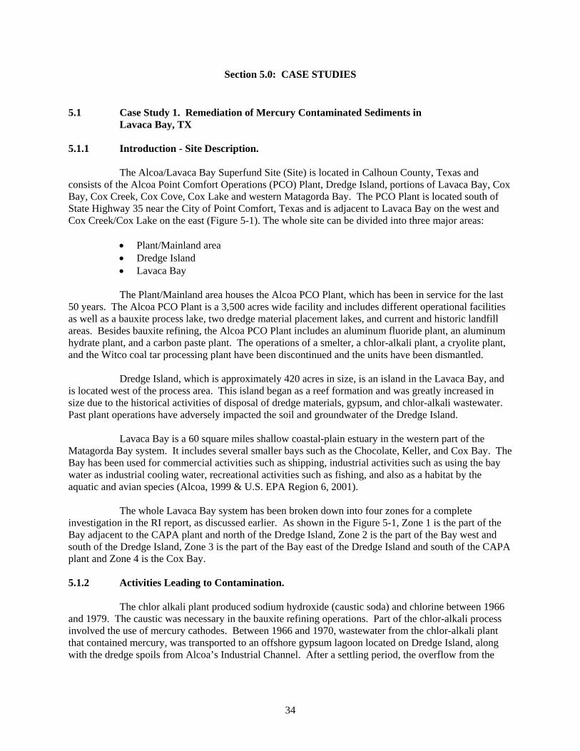
34

Section 5.0: CASE STUDIES 5.1 Case Study 1. Remediation of Mercury Contaminated Sediments in

Lavaca Bay, TX 5.1.1 Introduction - Site Description. The Alcoa/Lavaca Bay Superfund Site (Site) is located in Calhoun County, Texas and consists of the Alcoa Point Comfort Operations (PCO) Plant, Dredge Island, portions of Lavaca Bay, Cox Bay, Cox Creek, Cox Cove, Cox Lake and western Matagorda Bay. The PCO Plant is located south of State Highway 35 near the City of Point Comfort, Texas and is adjacent to Lavaca Bay on the west and Cox Creek/Cox Lake on the east (Figure 5-1). The whole site can be divided into three major areas:

• Plant/Mainland area • Dredge Island • Lavaca Bay

The Plant/Mainland area houses the Alcoa PCO Plant, which has been in service for the last 50 years. The Alcoa PCO Plant is a 3,500 acres wide facility and includes different operational facilities as well as a bauxite process lake, two dredge material placement lakes, and current and historic landfill areas. Besides bauxite refining, the Alcoa PCO Plant includes an aluminum fluoride plant, an aluminum hydrate plant, and a carbon paste plant. The operations of a smelter, a chlor-alkali plant, a cryolite plant, and the Witco coal tar processing plant have been discontinued and the units have been dismantled. Dredge Island, which is approximately 420 acres in size, is an island in the Lavaca Bay, and is located west of the process area. This island began as a reef formation and was greatly increased in size due to the historical activities of disposal of dredge materials, gypsum, and chlor-alkali wastewater. Past plant operations have adversely impacted the soil and groundwater of the Dredge Island. Lavaca Bay is a 60 square miles shallow coastal-plain estuary in the western part of the Matagorda Bay system. It includes several smaller bays such as the Chocolate, Keller, and Cox Bay. The Bay has been used for commercial activities such as shipping, industrial activities such as using the bay water as industrial cooling water, recreational activities such as fishing, and also as a habitat by the aquatic and avian species (Alcoa, 1999 & U.S. EPA Region 6, 2001). The whole Lavaca Bay system has been broken down into four zones for a complete investigation in the RI report, as discussed earlier. As shown in the Figure 5-1, Zone 1 is the part of the Bay adjacent to the CAPA plant and north of the Dredge Island, Zone 2 is the part of the Bay west and south of the Dredge Island, Zone 3 is the part of the Bay east of the Dredge Island and south of the CAPA plant and Zone 4 is the Cox Bay. 5.1.2 Activities Leading to Contamination. The chlor alkali plant produced sodium hydroxide (caustic soda) and chlorine between 1966 and 1979. The caustic was necessary in the bauxite refining operations. Part of the chlor-alkali process involved the use of mercury cathodes. Between 1966 and 1970, wastewater from the chlor-alkali plant that contained mercury, was transported to an offshore gypsum lagoon located on Dredge Island, along with the dredge spoils from Alcoa’s Industrial Channel. After a settling period, the overflow from the

35

gypsum lagoon was discharged to Lavaca Bay from two outfalls on Dredge Island between July 1965 to 1981 (U.S. EPA Region 6, 2001).

Figure 5-1. Site Location Map

5.1.3 Site Conceptual Model - Surface Hydrology. The Bay System at the site is a low-energy tidal system that is connected to the Gulf of Mexico through two small inlets. Saline water is brought into the bay by the industrial channel which brings in the water from the Gulf of Mexico. This water is mixed with the fresh water that is discharged from the rivers into the bay system. The saline water causes the vertical stratification of the water and also affects the circulation of the water near the Dredge Island. The long-term average current direction in the vicinity of the Dredge Island is counter-clockwise, as shown in Figure 5-2. Thus, if anything enters in the system near the CAPA, it follows the mean flow pattern and it moves northwards to the north of Dredge Island.

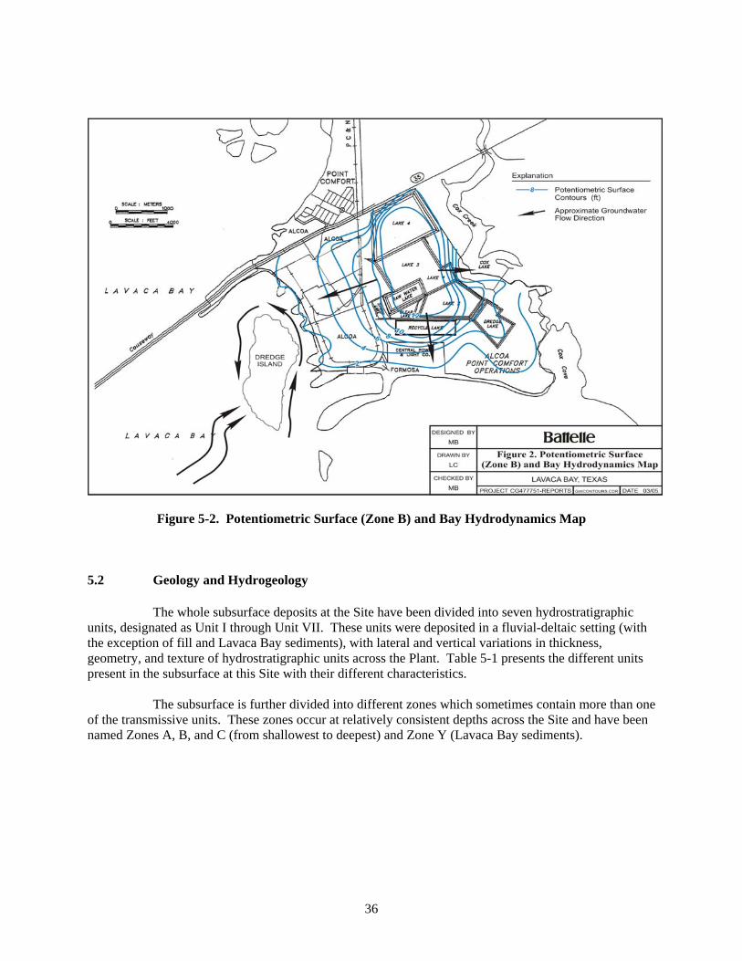
36

Figure 5-2. Potentiometric Surface (Zone B) and Bay Hydrodynamics Map

5.2 Geology and Hydrogeology The whole subsurface deposits at the Site have been divided into seven hydrostratigraphic units, designated as Unit I through Unit VII. These units were deposited in a fluvial-deltaic setting (with the exception of fill and Lavaca Bay sediments), with lateral and vertical variations in thickness, geometry, and texture of hydrostratigraphic units across the Plant. Table 5-1 presents the different units present in the subsurface at this Site with their different characteristics. The subsurface is further divided into different zones which sometimes contain more than one of the transmissive units. These zones occur at relatively consistent depths across the Site and have been named Zones A, B, and C (from shallowest to deepest) and Zone Y (Lavaca Bay sediments).

37

Table 5-1. Different Hydrostratigraphic Units Present in the Subsurface

and Their Characteristics

Unit Characteristics I (a) Hard Layers of gypsum and gypsum fragments with clay, silt, and sand I (b) Soft Clay with silt, sand, and shells

I (c) Excavated channel material consisting of Beaumont Formation Clay, silty clay, silt, and sand with minor Lavaca Bay sediments

II Beaumont Formation Clay, reddish brown to greenish gray in color and hard to medium toughness

III (a) Sand, silty sand, and sandy silt; sand is medium to fine grained III (b) Sandy silt, silty sand and silt; massive; minor clayey layers

IV Interbedded sand, silt, and clay rich layer; transitional unit between the sand rich and clay rich units

V(a)

Light gray, generally fining upward sequence ranging from fine-to medium-grained slightly silty sand near the base of the unit to a very silty to clayey, very fine-grained to fine-grained sand in the upper section; loose, massive to faintly laminated, well-sorted

V(b) Massive, hard, very silty to sandy clay to very clayey, sandy silt possessing a very light fray color and low plasticity

VI Well sorted, loose, very fine grained to fine-grained sand, thinly interbedded with clay and silty clay

VII Dark colored, soft, clayey silt and silty clay with shell fragments common 5.3 Zone A Zone A is mainly formed with Unit IV sediments of interbedded sand, silt, and clay with some Unit III sediments occurring as sub-linear, branching sand-rich bodies, the texture and geometry of which are more permeable than the Unit IV sediments and are representative of fluvial-deltaic and channel deposits. This zone was mostly encountered in the soil borings done in the Plant/Mainland area at an approximate elevation of up to 5 ft above mean sea level (msl). This Unit is overlain and underlain by the Beaumont Clay (Unit II). Zone A is said to have been removed completely from this area due to the construction of the Bauxite Residue lakes and the storm water lake. Groundwater in this zone is confined and discharges into the Bay system (mainly Lavaca and Cox). This zone has a steeper horizontal hydraulic gradient near the Bauxite Residue lakes and it decreases with the distances away from the lake. Vertical gradient in this zone is downward. Recharge comes through these lakes with some participation from the direct precipitation and leakage from the water lines. Groundwater has a high value of total dissolved solids (TDS) near the bay shoreline (>10,000 mg/L) and a lower TDS near the lakes. This high salinity has rendered the water non-potable in this area. 5.4 Zone B Zone B is separated from Zone A by Unit II sediments. This zone includes Unit V(a) and Unit V(b) sediments with pockets of Unit IV sediments, and consists of massive sequences of silty sand and well-graded sand. Zone B is mostly found in the Plant/Mainland area and is located at an elevation of -20 to -30 ft msl. Zone B is the principal stratigraphic unit that conveys groundwater flow from the

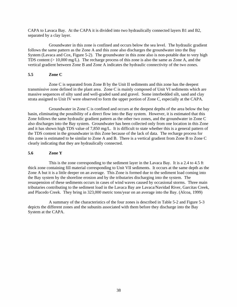
38

CAPA to Lavaca Bay. At the CAPA it is divided into two hydraulically connected layers B1 and B2, separated by a clay layer. Groundwater in this zone is confined and occurs below the sea level. The hydraulic gradient follows the same pattern as the Zone A and this zone also discharges the groundwater into the Bay System (Lavaca and Cox, Figure 5-2). The groundwater in this zone also is non-potable due to very high TDS content (> 10,000 mg/L). The recharge process of this zone is also the same as Zone A, and the vertical gradient between Zone B and Zone A indicates the hydraulic connectivity of the two zones. 5.5 Zone C Zone C is separated from Zone B by the Unit II sediments and this zone has the deepest transmissive zone defined in the plant area. Zone C is mainly composed of Unit VI sediments which are massive sequences of silty sand and well-graded sand and gravel. Some interbedded silt, sand and clay strata assigned to Unit IV were observed to form the upper portion of Zone C, especially at the CAPA. Groundwater in Zone C is confined and occurs at the deepest depths of the area below the bay basin, eliminating the possibility of a direct flow into the Bay system. However, it is estimated that this Zone follows the same hydraulic gradient pattern as the other two zones, and the groundwater in Zone C also discharges into the Bay system. Groundwater has been collected only from one location in this Zone and it has shown high TDS value of 7,850 mg/L. It is difficult to state whether this is a general pattern of the TDS content in the groundwater in this Zone because of the lack of data. The recharge process for this zone is estimated to be similar to Zone A and B. There is a vertical gradient from Zone B to Zone C clearly indicating that they are hydraulically connected. 5.6 Zone Y This is the zone corresponding to the sediment layer in the Lavaca Bay. It is a 2.4 to 4.5 ft thick zone containing fill material corresponding to Unit VII sediments. It occurs at the same depth as the Zone A but it is a little deeper on an average. This Zone is formed due to the sediment load coming into the Bay system by the shoreline erosion and by the tributaries discharging into the system. The resuspension of these sediments occurs in cases of wind waves caused by occasional storms. Three main tributaries contributing to the sediment load in the Lavaca Bay are Lavaca/Navidad River, Garcitas Creek, and Placedo Creek. They bring in 323,000 metric tons/year on an average into the Bay. (Alcoa, 1999) A summary of the characteristics of the four zones is described in Table 5-2 and Figure 5-3 depicts the different zones and the subunits associated with them before they discharge into the Bay System at the CAPA.

39

Table 5-2. Summary Table of Different Zones and Their Characteristics

Zone Units found Thickness Location

Groundwater Characteristics and

Direction Recharge Zone

A IV and III underlain by unit II sediments

maximum-15.8-ft average thickness- 4-ft

5 to 0 ft msl confined; discharges into the Lavaca and Cox Bay

Precipitation, surface impoundments and leaking water lines

B

Separated from Zone A by Unit II sediments, includes Units V(a) and V(b) sediments

1-ft to greater than 20-ft

-20 to -30 ft msl

confined; discharges into the Lavaca and Cox Bay

Precipitation, surface impoundments and leaking water lines

C

Separated from Zone B by Unit II sediments, includes Unit IV sediments

Not Known deepest transmissive zone

confined; no data available for exact location of discharge but assumed to follow the direction of zone B

Precipitation, surface impoundments and leaking water lines

Y Lavaca Bay sediments; Unit VII

2.4-ft to 4.5-ft thick

Same interval as Zone A but a little deeper

NA NA

Msl: mean sea level NA: Not Applicable

Figure 5-3. Geological Sub-Units: I, II, III, IV, V, VI, and VII

40

5.7 Chemicals of Potential Concern The chemicals of potential concern (COPCs) identified for this site are mercury and polynuclear aromatic hydrocarbons (PAHs). Though it is difficult to estimate the concentrations of the COPCs in sediments, it is generally considered to be high. This is the reason that the data is compared to Effects Range Low (ERL) and Effects Range-Median (ERM) to determine whether it is above or below the level it should be present in the nature. Apparent Effect Threshold (AET) values for benthic organisms are also reported. AET is the highest “no-effect” concentration for a contaminant on a particular organism. The ERL and ERM concentrations are the lower (10 percentile) and median (50 percentile) of the concentrations associated with toxic effects (NOAA, 1996). The ERL and ERM values together define the concentration ranges that were (1) rarely, (2) occasionally, and (3) frequently associated with adverse effects (Alcoa, 1999). The ERL for mercury is 0.15 mg/Kg of sediments or 0.15 ppm and ERM is 0.71 ppm (NOAA, 1996) and the AET is 2.1 ppm (Baumgarten, 2001). For PAHs, the ERL and ERM in sediments are 4.022 ppm and 44.792 ppm respectively (Alcoa, 1999). 5.8 Sources of Contamination Based on the subsurface investigations conducted till date, the Remedial Investigation (RI) report prepared by Alcoa indicates that the highest surface sediment concentrations of mercury occurred along the CAPA shoreline. The concentrations of mercury in the sediments in this area ranged from 10 to 50 ppm with some individual samples exceeding 100 ppm of mercury. In general, concentrations of the COPCs peaked immediately below the sediment surface. Concentrations reverted back to the pre-CAPA concentrations with increase in depth. The peak was attributed to the wastewater discharge from the CAPA operations in the 1960s and early 1970s. The scenario changed for the sediments near the shoreline of CAPA where the elevated concentrations remained for a longer interval (20 to 100 cm) after the at-depth peak concentration of mercury was reached. This indicated that apart from the wastewater discharge from CAPA in the 1960s and 1970s, there was also another source of ongoing contamination. Upland groundwater investigations determined that the elevated concentrations of dissolved mercury in the groundwater in that area were attributable to the discharge from the Zone B water bearing sand into the Bay system adjacent to the CAPA. Alcoa, based on the characterization studies, estimated in the RI report that the mercury loading of the area due to this groundwater discharge ranged from 0.5 pounds to 90 pounds per year. An additional source responsible for elevated surface concentrations of mercury in these areas is surface water runoff from the Dredge Island. Alcoa, through a combined monitoring and modeling approach, in the RI report has estimated that 8 to 13 pounds of mercury per year are introduced into the Bay as a result of runoff from the northern areas of Dredge Island. Another potential source contributing to the elevated surface mercury concentrations is the resuspension of contaminated sediments due to ships and barge traffic. This is a potential concern for areas off-site of the CAPA, where high surface sediment concentrations exist and also for the Witco channel. These areas have elevated levels of mercury either because of the on-going sources of mercury or because of the historical CAPA wastewater discharge. Witco area is also the source for another COPC (PAH) for the Bay system (Alcoa, 1999 & U.S. EPA Region 6, 2001).

41

5.9 Aerial and Vertical Extent of Mercury Contamination in Lavaca Bay Sediments Figure 5-4 and 5-5 exhibit the aerial as well as vertical extent of mercury concentrations in the sediments.

Figure 5-4. Mercury Concentrations in the Sediments in the First Five Centimeters Where Mercury is Present as Methyl Mercury Concentration With High Concentrations. The small land

portion in the Bay System is the Dredge Island. It can be easily observed from the figure that the concentrations are the highest near the CAPA shoreline. (Baumgarten, 2001)

42

Figure 5-5. Mercury Concentrations in the Sediments in the 5-30 Centimeters. The small land portion in the Bay System is the Dredge Island. It can be easily observed from the figure

that the concentrations are the highest near the CAPA shoreline and the north of Dredge Island. (Baumgarten, 2001)

Sediments adjacent to the CAPA (major source of mercury contamination in the Lavaca Bay system) or in the Zone 1 exhibit elevated concentration of mercury (average surface concentration being 1.7 ppm). In particular, the highest concentrations are observed near the CAPA shoreline (average concentration being 13.6 ppm as shown in Figure 5-4 and 5-5) and the north of the Dredge Island. As stated earlier, the direction of water flowing in this area is counter-clockwise resulting in the transport of the contamination emanating from the CAPA towards the north and the north-west of the Dredge Island; consequently elevating the mercury levels in the sediments in this area. The surface water run-off from the Dredge Island also contributes to the elevated levels of mercury in this area. The extent of mercury contamination decreases as the distance from the CAPA area increases. Mercury levels in the Zone 2, south and west of the Dredge Island were in the range of 0.37 ppm and 4.6 ppm. The elevated levels in the region are associated with a historic dike failure on the Dredge Island. Zone 3 and 4 show relatively lower range of mercury levels in the range of 0 to 0.5 ppm. Vertical extent of mercury in the whole Bay system varies greatly with depth. Sedimentation in the area has greatly influenced the vertical extent of mercury concentration. This is also the reason for the concentration to be high at a certain depth at different location in the Bay area. Sedimentation, erosion and re-suspension have led to a depth profile of mercury in the sediments. Investigators have observed that a certain depth of the sediment has the highest concentrations, and the concentration of mercury decreases steadily after that. Such stratification is due to physical processes, such as sedimentation.

43

The sediments in the Zone 1 have a peak concentration above 100 ppm at varying depths but there are no discernible points at which the level of mercury concentration goes down. The average concentration thus for the area near the CAPA shoreline is 44.6 ppm, which is higher than the AET (shown in Figure 5-4 and 5-5). In the north of Dredge Island, the mercury levels have been found to be much lower near the Alcoa facility averaging around 2.7 ppm but higher than AET ( as shown in Figure 5-4 and 5-5) with the mercury concentration going down between the depths of 30 and 70 cm. Mercury concentrations in Zone 2 have been found to be below 0.7 ppm but in the area west of Dredge Island the concentrations went up again and were between 13 and 14 ppm for two locations in this area, as seen in the Figure 5, where there are some areas with higher mercury concentrations in the southwest of Dredge Island. The concentrations of mercury decreased again in these locations at depths between 15 and 50 cm. The concentrations were further lower in the Zone 3, averaging around 0.33 ppm. There was a rise in the mercury levels in sediments in Zone 4 with the levels being in the range of 0.57 to 6.1 ppm in the area south of Calhoun County Navigational District (CCND) with various depths at which they went down again. In the middle of Cox Bay the range of mercury levels in the sediments was around 0.5 to 3.24 ppm with the levels gradually going down at depths between 50 and 70 cm. (Alcoa, 1999). 5.10 Extent of PAH contamination in the Lavaca Bay System PAH contamination has been observed to be high in the Zone 1, similar to mercury contamination, with the highest concentration encountered being 581.38 ppm. The difference between the two COPCs is that no other zone than Zone 1 has been found to contain any PAH contamination. Thus, this chemical is localized only to Zone 1 near the CAPA shoreline and is not a problem in the north of Dredge Island. 5.11 Sampling Events Alcoa conducted various extensive sampling events in the Lavaca Bay area which included pore-water sampling (Mason et. al., 1998), Bay water column sampling, Bay sediment sampling, groundwater sampling in the plant/mainland area, soil sampling in the same area, and even air sampling to detect if mercury present in the area was volatilizing. Results of these sampling helped in determining the extent and location of mercury contamination in the area. Some of the sampling and modeling events which stand out were the sediment radiochemistry data for finding the sedimentation rate in the Bay system and the Hurricane Scour Model. These studies were important as they helped in determining the remedial strategies for this area. 5.11.1 Alcoa Radiochemistry Study Report. Surface Radiochemistry data entailed an isotopic study to determine the age of all sediment cores. It was accomplished by analyzing the profiles of the atmospherically delivered nuclides 137Cs, and, in some cases 239, 249 Pu (bomb fallout peak in 1963), and 210Pb (half-life of 22 years, steady delivery). The study determined that sediment accumulation rates were the highest in Cox Bay, in sediments from the shoreline of the CAPA, and north of Dredge Island, and generally decreases away from these sites Mixing of sediments due to bio-perturbation, benthic organisms or sediment resuspension was also analyzed. The study showed that the mixing was localized in the shallow regions of the sediments (<10 cm) by all the above mechanisms and even due to the burrowing organisms, leaving the sediments below them undisturbed. It was observed that the mixing was generally restricted to the 2 to 5 cm of the sediment layer with greater depths of 10 cm occurring in summer, with them being higher south of the Lavaca Bay and in Keller Bay. (Alcoa, 1998).

44

5.11.2 Hurricane Scour Model. The Hurricane Scour Model developed by HydroQual used Hurricane Carla as the design storm event. The model predicted that the surficial mercury concentrations in the Bay would not increase in the case of a hurricane. On the contrary, it showed that in several locations the mercury concentration would subside due to redeposition of less contaminated solids. The average net erosion depth was found to be less than 5 cm in about 70 percent of the Bay; and only 2 percent of the Bay was found to have scour depths greater than 10 cm. These areas which were vulnerable to erosions were the ones where water depth, current velocity and substrate type were such that significant erosion could occur (Hydroqual, 1998). 5.12 Risk Assessment Studies The Mercury Reconnaissance Study Report as part of the RI report delves into the details of bioavailability of mercury in the estuarine ecosystem. In conformity to the previous research, the report finds that methyl mercury, which is the most bioavailable form of mercury, is predominantly present in the first 5 cm of the sediments. The methyl mercury, generally produced by the sulfate reducing bacteria, is taken up by the benthic invertebrates as a carbon source from where it moves up to the upper echelons of the food chain. The investigation of mercury present in the red drum and black drum fish demonstrated that they feed on the Crustacea and other small fish which dominate the marsh areas and pick up mercury from the sediments, thus making sediments as the primary source of mercury contamination in the Bay area. Avian species, which fed on fishes, snails, amphipods etc. found in the Bay area, had elevated levels of mercury in their tissue (Alcoa, 1996). No direct relation was found between the methyl mercury present in the area and the mercury levels in the zooplankton, but the study demonstrated that areas with high methyl mercury in sediments were the areas where mercury was finding its way in the food chain due to methyl mercury being picked up by the benthic organisms like the invertebrates, amphipods etc. The concentrations of total and methyl mercury in sediments, pore water, and the biota were higher near the Alcoa plant than the other areas. Figures 5-6 and 5-7 depict this with data drawn from tissue of red drum and black drum fishes, clearly indicating that the area in close proximity to the facility was the source of most of the mercury that is finding its way into the Lavaca Bay system. The total mercury levels in the overlying water were also higher near the Alcoa plant facility.

45

Figure 5-6. Mercury Concentrations in Black Drum Fish Tissue. Mercury concentrations were the highest near the CAPA shoreline in zone 1 (Baumgarten, 2001)

Figure 5-7. Mercury Concentrations in Red Drum Fish Tissue. Mercury concentrations were the highest near the CAPA shoreline in zone 1 (Baumgarten, 2001)

The reconnaissance report also demonstrated that the mercury present in the water columns which bears the whole biosystem of the area is also supplied by the sediments. It was found that the particulate methyl mercury concentrations in the system were directly correlated to the presence of methyl

46

mercury in the sediments. The enrichment in the particulate fraction of mercury was attributed to the resuspension effects of wind driven events, which preferred the fine grained sediments. It has been reported in the RI report that the levels of mercury in the biota of the Bay system is going down with time clearly indicating that the control of mercury pollution in the area has been helping the Bay area towards a better future (Alcoa, 1996). 5.12.1 Mercury Speciation is Sediments. Mercury exists as three oxidation states: elemental mercury, Hg0; mercurous ion, Hg2

2+; and mercuric ion, Hg2+. In natural systems, the Hg2+ species generally predominates. It has been observed that in oxidizing conditions in freshwater, inorganic mercury is predominately present as Hg(OH) 2 and HgOHCl, and in the reducing conditions the sulfur based mercury species such as HgS are primarily present but in the marine systems mercury complexes with the chloride (Cl-) present to form soluble HgCl4

2-. Mercury also complexes with the humic and organic matter present in the aquatic systems but this phenomenon is subdued in the marine waters because of the presence of abundant Cl- ions. Thus, in Lavaca Bay, mercury predominately exists in Hg0, Hg(OH) 2 and HgOHCl formed in the oxidizing conditions, and as HgS in the reducing environment, but apart from these mercury is also found to exist as organomercury species, monomethyl mercury (CH3Hg+) and dimethyl mercury ([CH3]2Hg). The transformation of mercury between the elemental form, the ionic form and the organomercury is controlled by biotic and abiotic processes in aerobic and anaerobic environments. Methyl mercury is generally a product of methylation of inorganic mercury carried out by the sulfate reducing bacteria in the aquatic environments rather than abiotic processes (Bloom, et. al., 1999).

Research has shown that in a stratified estuarine environment such as Lavaca Bay, monomethyl mercury concentrations are highest at the oxic/anoxic interface of the sediment system or in the first 5 cm of the sediment layer (Bloom, et. al., 1999). This finding seems to apply to Lavaca Bay. The production of organomercury is a problem as this is the predominant bioavailable form of mercury which eventually is taken up by the flora and the fauna of the aquatic ecosystems. and bioaccumulates at every step of a common food chain of the system thus making mercury available to the upper echelons of food chains, possibly making humans as an end receptor to mercury contamination. In the Lavaca Bay area it was also observed that the monomethyl mercury concentrations were high in the marshes. These marshes are highly productive environments with detrital carbon (plant litter) which drive the microbial process which promotes methylation of the bioavailable mercury. The higher mercury levels in these areas indicated that these were the areas where mercury was being transferred into the food chains as most of the higher tropic level organisms feed on the lower trophic level organisms found in these areas. The lower organisms on the lower levels of the food chain pick up their mercury from the sediments of these areas (Alcoa, 1996). 5.13 Risk Characterization Risk characterization was based on the combination of the exposure assessment and toxicity assessment of the sediments using tools like Excess Lifetime Cancer Risks (ELCR) and Hazard Index (HI). ELCR are determined for each exposure pathway by multiplying a daily intake level with the chemical specific cancer potency factor, developed by U.S. EPA to reflect a conservative “upper-bound” of the risk posed by potentially carcinogenic compounds. The acceptable risk range of ELCR for a site related exposure by U.S. EPA is 10-4 to 10-6. Current U.S. EPA practices considers carcinogenic risks to be additive when assessing exposure to a mixture of hazardous substances. In assessing the potential for adverse effects other than cancer, a hazard quotient (HQ) is calculated by dividing the daily intake level by the reference dose (RfD), developed by U.S. EPA representing a level to which an individual may be exposed that is not expected to result in any deleterious effect. A HQ less than or equal to 1 (<1)

47

indicates that a receptor's dose of a single contaminant is less than the RfD, and that toxic noncarcinogenic effects from that chemical are unlikely. The HI is generated by adding the HQs for all chemical(s) of concern that affect the same target organ (e.g., liver) within or across those media to which the same individual may reasonably be exposed. A HI < 1 indicates that toxic noncarcinogenic effects are unlikely.

The risk characterization carried out in the Plaint/Mainland area and the Dredge Island indicated that the associated ELCR and HI were both below the levels of concern in these areas with the exposure pathways being incidental ingestion and also dermal contact, except in areas near the R-300 building at CAPA, where HI was greater than 1 based on Industrial exposure scenarios by incidental ingestion. Risk characterization for the Bay area was more exhaustive due to direct fish consumption which increases the chances of bioaccumulation/biomagnification of methyl mercury. For the site, HI and ELCR were calculated using a RfD dose of 0.1 µg/kg per day, a toxicity value determined by EPA. HI were all calculated based on the average fish consumption rate of 24 grams/day and the reasonable maximum exposure (RME) of 45 grams/day. The current U.S. EPA RfD suggests that the women who consume fish from Lavaca Bay at the RME fish consumption rate could put their unborn child at risk for potential neurodevelopmental effects. This was not true for average fish consumption rates which had HI<1 with an exception that the fish was being caught from the closed area in the Lavaca Bay, near the facility. There are uncertainties attached to all the risk characterizations conducted in the area, for example, the RfD is an estimate with the uncertainty spanning to an order of magnitude, of a daily exposure to the human population that is likely to be without appreciable risk during a lifetime (U.S. EPA Region 6, 2001). 5.14 Ecological Risk Assessment The potential exposure pathways for the ecological receptors at the site were direct contact with mercury and PAH in sediments for benthos, indirect contact with chemicals detected in ground water that may be transported to Lavaca Bay, direct contact with mercury in surface water for zooplankton, direct contact with mercury in sediments for larvae stages of fish, and bioaccumulation/biomagnification of methyl mercury and ingestion of contaminated prey for fish and birds.

The risk assessment suggested that the portions of the Bay near the Witco and CAPA had sufficient concentrations of PAH to pose potential for localized impacts on benthic survival and reproduction. For fish in the Lavaca Bay, it was found that the mercury tissue concentration posed a potential risk for behavioral and reproductive effects. But food exposure models suggested that bioaccumulation in higher tropic level organisms was below levels of concern in fish as well as the avian species. Although, qualitative estimation of overall risk posed by the mercury contamination suggested that the sediment concentration of mercury in the areas north and east of Dredge Island could pose a possible risk. In the plant/mainland area, risk was posed to the mammals and birds found in the area due to the heavy PAH compounds found in the area. Detritivores were found at risk in the Dredge Island due to exposure to mercury concentrations in soil in this area (Alcoa, 2001).

Finally, the risk assessment showed the following potential noncarcinogenic hazard indices greater than one, cumulative excess carcinogenic risks exceeding 1 × 10-4, and environmental impacts:

(1) Noncarcinogenic risk to a future industrial worker, future construction worker, and current maintenance worker exposed to mercury-contaminated soils within the footprint of the R-300 building;

(2) Noncarcinogenic risk to a woman of childbearing age consuming fish from within Lavaca Bay and the Closed Area of Lavaca Bay;

48

(3) Carcinogenic risk to a future industrial worker in the Witco Area; and

(4) Ecological impacts. Table 5-3 summarizes the risk characterization of the whole site. 5.15 Remedial Action Objectives The remedial action objectives (RAOs) for this site are area-specific. Different RAOs are present for the Lavaca Bay area, CAPA, and Witco area. 5.15.1 Lavaca Bay. The RAOs for Lavaca Bay are to:

(1) Eliminate or reduce the maximum extent of practical mercury loading from on-going unpermitted sources to Lavaca Bay;

(2) Reduce to an appropriate level of mercury in surface sediments in sensitive habitats; and

(3) Reduce to an appropriate level of mercury in surface sediments in open-water that represent a pathway by which mercury may be introduced into the food chain.

The RAOs for mercury in sediment have two quantitative target cleanup goals, depending on the location of the sediment. The target cleanup goals are:

• For sediments in fringe marsh-type habitat, eliminate the exposure pathway that is presented by sediments that on an average exceed 0.25 ppm of mercury.

• For sediments in open-water habitat, eliminate the exposure pathway that is presented by sediments that on an average exceed 0.5 ppm of mercury.

Lower values are adopted for the marshy areas as the risk assessment study has shown that the methyl mercury uptake is almost twice as high as other areas in these areas. The specific target sediment cleanup value for critical habitats (fringe marsh-type), 0.25 ppm mercury, is based on a weight-of-evidence evaluation of empirical measurements of the ratio of tissue-to-sediment concentration determined during the RI phase of the project and long-term tissue monitoring data. It is predicted that achieving these goals would lead to reduction of mercury in the fish tissue such that there are no unacceptable risks to ecological receptors even for the most conservative risk estimate. The target sediment goal of 0.25 ppm mercury for fringe marsh-type habitat is expected to reduce mercury in fish tissues of the smaller resident species, such as that noted for killifish within marshes in the Closed Area to the north and east of Dredge Island, and below the 0.5 ppm mercury tissue level noted for potential behavioral effects. The target sediment goals of 0.25 ppm mercury for fringe marsh-type habitat and 0.5 ppm mercury for open water is expected to result in mercury concentrations below the 2 ppm mercury concentration noted for fish tissue that relates to adverse effects in survival and reproduction for large predatory carnivorous fish.

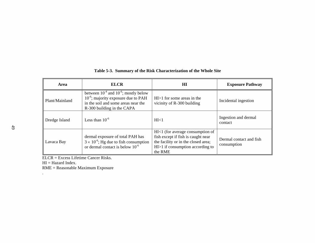
49

Table 5-3. Summary of the Risk Characterization of the Whole Site

Area ELCR HI Exposure Pathway

Plant/Mainland

between 10-4 and 10-6; mostly below 10-6; majority exposure due to PAH in the soil and some areas near the R-300 building in the CAPA

HI>1 for some areas in the vicinity of R-300 building Incidental ingestion

Dredge Island Less than 10-6 HI<1 Ingestion and dermal contact

Lavaca Bay dermal exposure of total PAH has 3 × 10-6; Hg due to fish consumption or dermal contact is below 10-6

HI<1 (for average consumption of fish except if fish is caught near the facility or in the closed area; HI>1 if consumption according to the RME

Dermal contact and fish consumption

ELCR = Excess Lifetime Cancer Risks. HI = Hazard Index. RME = Reasonable Maximum Exposure .

50

5.15.2 Chlor Alkali Process Area. The general RAO for CAPA soils is to reduce the future exposure potential of site workers (e.g., construction worker, general industrial worker, and maintenance worker) to mercury in soils in the Building R-300 vicinity. The exposure pathways considered here are incidental ingestions and dermal contact. The RAO for CAPA soils does not include reducing the potential for ongoing leaching of mercury from these soils to underlying groundwater, since control of CAPA ground water discharge to the bay will be performed as part of the Bay remedial action alternative. 5.15.3 Witco. The RAO for soils in the Witco Area is to reduce the future exposure potential of site workers (e.g., construction worker, general industrial worker, and maintenance worker) to PAHs in surficial soils at the Stormwater Sump and Separator Area and Former Tank Farm Area. The exposure pathways considered when developing the RAO are incidental ingestion and dermal contact with soils. For the seven carcinogenic PAHs, the following preliminary remediation goals are presented as cleanup levels for the Witco Area soils (Alcoa, 2001; U.S. EPA Region 6, 2001).

Benz(a)anthracene 32 mg/kg Benzo(a)pyrene 3.2 mg/kg Benzo(b)fluoranthene 32 mg/kg Benzo(k)fluoranthene 320 mg/kg Chrysene 3200 mg/kg Dibenz(a,h)anthracene 3.2 mg/kg Indeno(1,2,3-c,d)pyrene 32 mg/kg

5.16 Selected Remedies for the treatment of Lavaca Bay sediments As part of the remedial program at the Lavaca Bay, Alcoa has already conducted some of the remedial actions agreed upon in the record of decision (ROD). There is a pump-and-treat system already in place at the CAPA, which extracts groundwater from this area and treats it by passing the groundwater through granular activated carbon (GAC). Sediments from the CAPA shoreline having high mercury concentrations have been dredged and disposed off in the dredge lakes. Dredge materials are being stabilized by transferring them to the gypsum placement areas on the dredge island where the material is surrounded by 10,700-ft of linear dikes with an elevation of 30-ft. Different areas discussed here are also shown in Figure 4. Other technologies which were agreed upon in the ROD are: 5.16.1 Installation of a DNAPL Collection or Containment System at the Witco Area. West of the former Witco Tank Farm Area, a collection trench or containment system will be installed for the purpose of intercepting DNAPL potentially migrating to Lavaca Bay. Recovered DNAPL will be collected and sent off site for treatment and disposal at a licensed disposal facility. The DNAPL will not be treated or stabilized on site prior to off site disposal. The specific areas of shoreline to be addressed by a remedy may be modified based on site conditions observed during remedy implementation. The use of either a DNAPL containment or collection technology will be refined during the remedial design. 5.16-2 Dredging of the Witco Channel. Approximately 200,000 cubic yards of mercury contaminated sediment will be dredged and disposed of in an on site confined disposal facility located on Dredge Island. The dredged sediments will

51

not be treated or stabilized before disposal. A final cover for the disposal areas will consist of dredged material taken from an area of Lavaca Bay that has mercury concentrations below human health and ecological risk-based values. 5.16.3 Remediation of the Witco Marsh by Dredging. The Witco Marsh would be actively remediated to address the concern of biological uptake of mercury. Around 38,000 cubic yard of sediments would be dredged from this area and disposed off on the disposal cells on the dredge island. Effort will be made to minimize the transport of the dredge materials to other locations by monitoring the total suspended solids. 5.16.4 Enhanced Natural Recovery North of Dredge Island. The areas north of Dredge Island (shown in Figure 3) would receive a thin cap over the entire area to accelerate the natural recovery process currently observed occurring in Lavaca Bay. The in-situ cap will consist of sediments taken from a location which don’t have mercury contamination. It is supposed to be 15 centimeters in thickness. This technology was found useful based on the Alcoa Radiochemistry report and also the Hurricane Scour model which, as mentioned above, reported that the mixing of sediments occurred only in the upper 10 cm of the sediments and below this depth the sediments remained undisturbed. Scour model predicted that the erosion in the area will never scour more than 10 cm of sediments even in the case of a strong Hurricane rendering the sediments below the cap totally undisturbed in any case. The Radiochemistry study had also reported higher sedimentation rates in this area. 5.16.5 Natural Recovery of Sediments. Sediments that are not actively remediated will recover to acceptable levels through natural sedimentation. It is estimated that surficial sediment mercury levels in all areas are expected to decline to levels in the current range of open areas of the Bay within a 5 to 10 year time frame. Sedimentation studies conducted through the Hurricane Scour Model and Surface Radiochemistry have suggested that this timeline is appropriate enough to consider a natural recovery rate of the sediments mainly by the effects of burial. 5.16.6 Monitoring. Long term monitoring of sediments and fish will be required to confirm the natural recovery of sediment and fish tissue to acceptable levels. In addition, monitoring of surface water will be conducted to evaluate the effectiveness of the CAPA hydraulic containment system. Full details of the monitoring program will be established during the design of the selected Bay System remedy. 5.16.7 Removal of Building R-300 and Capping the Area. The walls and roof of Building R-300 (shown in Figure 5-8) will be removed and hauled off-site. The building slab and the area immediately west of Building R-300 will be capped with a clay sub layer covered by crushed rock.

52

Figure 5-8. Site Map 5.16.8 Capping of the Witco Soil. The Storm Water Sump and Separator Area and Former Tank Farm Area will be capped with soil caps. 5.16.9 Institutional Controls to Manage Exposure to Finfish/Shellfish. The fish closure originally established by the Texas Department of Health in 1988 and updated in January 2000 will remain in place to control the consumption of finfish and shellfish for the “Closed Area”. 5.16.10 Institutional Controls to Manage Exposure to Soil. Excavation of any soils below or immediately west of Building R-300 would only be permitted after a worker safety program is developed for the specific excavation activity and repair of the cap would be required after excavation. The Building R-300 area would be deed recorded as containing soils with elevated mercury and PAH levels (Alcoa, 2001; U.S. EPA Region 6, 2001; Alcoa, 2000; Alcoa, 2003).

53

5.17 Lessons Learned By the overview of the documents provided to us, it is clear that the site is recovering and the affirmative results of measures taken by Alcoa are visible in the recent analytical tests reported. The selected remedies in the ROD should be able to restore the site, but there are certain research areas which, if delved into can prove useful in future research and understanding of mercury contaminated sites. This site can prove as a guiding case study for further investigation in the issues still not very clear while dealing with mercury contamination in sediments. We have tried to touch upon some of these issues by our understanding of the documents provided to us. Based on the data collected from the Lavaca Bay, it has been observed that mercury concentrations in water above contaminated sediment vary between seasons. It has been observed that the concentration in the winter season are generally lower in the same water column locations that in summer months, clearly indicating a trend of temporal variations in mercury concentrations. In order to understand such temporal variations in concentrations, Alcoa has monitored the mercury concentrations in biota, sediments and water column. Evaluation of the analytical data has explained the historical reduction in the total mercury concentrations in the sediments. Therefore, temporal variation in mercury concentrations in water column above contaminated sediments is a pertaining issue. A further study on the seasonal variation of mercury in the Lavaca Bay water covering all the impacted areas can shed some more light on our understanding of fate and transport of mercury in an estuarine environment and also on its bioavailability. The fate and transport of mercury in the environment is greatly influenced by the biogeochemistry of mercury, as this affects the speciation of mercury in an aquatic environment. Understanding of the biogeochemistry is also an important issue as this is an essential part of any remediation work which can be undertaken anywhere for mercury contaminated sediments. The understanding of mercury speciation, based on Alcoa’s studies, resulting from the biogeochemical reactions in the sediments of Lavaca Bay is extensive, and has been studied in great details by many researchers (Gill, et. al., 1999; Santschi, et. al., 1999). Additional long-term investigation in the biogeochemistry via a long term monitoring program can prove helpful in shedding more light on mercury transportation after conditions of enhanced natural recovery are set forward. Such a study is most suitable for the area north of dredge island where the in-situ capping is to be done. Battelle thinks that the dredge lake, which is the location for disposal of dredged mercury sediments, is another important area of investigation. It will be an appropriate location to model the fate of mercury on a long term basis. As part of the future monitoring program, Alcoa plans to do the needful for recovery and monitor the decant water, which is a part of the dredged sediments and transporting it back to the Bay once it is restored. Alcoa also plans on placing a cap on these dredged materials. Another appropriate area of investigation pertaining to the fate of mercury is evaluating the mercury concentrations in these disposal areas by sampling at various depths and conducting an ecological assessment of the area. A major issue in this study was EPA’s RfD for mercury. As mentioned earlier, U.S. EPA has set a reference dose of 0.1 µg/kg of body weight/day as an amount that can be ingested by a human over a lifetime without producing adverse health outcomes. This dose is still an issue of debate among the scientific community. S. Allen Counter and Leo H. Buchanan in their review paper on mercury exposure in children report that studies have suggested that a food preparation factor should also be used in risk characterization apart from the RfD as when the fish is cooked (especially by deep-frying), the concentration of mercury increases, although the cooked fish retains the same amount or mass of mercury as raw fish. They also report a benchmark dose recommended by the National Academy of Sciences (NAS), which is 5.8 µg/L in cord blood (Counter et. al., 2004). Another study by Deborah C. Rice argues that the derivation of RfD for methyl mercury is inappropriate. The report gives various reasons for their comment including a contradiction on the use of value of 10 as an uncertainty factor (Rice, 2004). Even

54

Alcoa, according to the RI report and ROD, have conducted their own study for the RfD and came up with a different value. Battelle thinks it would be appropriate for our future understanding to go into the details of the RfD and its appropriateness as a universal value and also on the issue that whether we require case-specific value for RfD for conducting a risk characterization study due to the presence of methyl mercury (Alcoa, 1999). Battelle agrees with Alcoa that there is a need for future research on the movement of elemental mercury present in the CAPA subsurface and determining whether it is migrating towards the Bay System. Further research into the appropriation of the hurricane scour model might also prove beneficial to investigate as further calibration using some recent hurricane or storm data might prove useful apart from the use of Hurricane Clara of the year 1961. Finally, it is clear from the documents provided to us that Alcoa has done extensive research on this site and their treatment efforts have proven successful in mitigating the problem. Above-identified research needs can act as a furtherance to the existing wealth of information and can help the scientific community at large for a more detailed understanding of mercury contamination, and possible outcomes of the remediation activities which can be undertaken, keeping Lavaca Bay as an exemplary case study. 5.18 Case Study 2. Sediment Stability Model to Empirically Determine

Mercury Budget in Onondaga Lake, New York The sediments of Onondaga Lake, a hypereutrophic lake in Syracuse, New York (Figure 5-9), are extensively contaminated with mercury as well as many other contaminants.

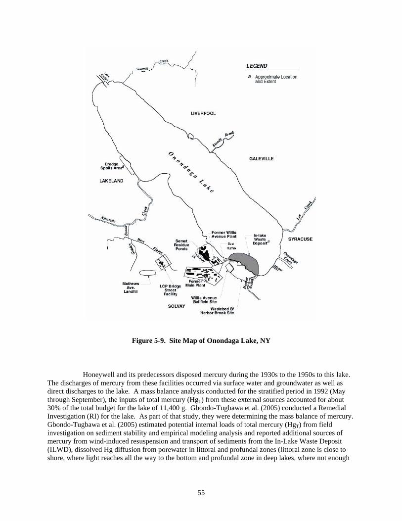
55

Figure 5-9. Site Map of Onondaga Lake, NY

Honeywell and its predecessors disposed mercury during the 1930s to the 1950s to this lake. The discharges of mercury from these facilities occurred via surface water and groundwater as well as direct discharges to the lake. A mass balance analysis conducted for the stratified period in 1992 (May through September), the inputs of total mercury (HgT) from these external sources accounted for about 30% of the total budget for the lake of 11,400 g. Gbondo-Tugbawa et al. (2005) conducted a Remedial Investigation (RI) for the lake. As part of that study, they were determining the mass balance of mercury. Gbondo-Tugbawa et al. (2005) estimated potential internal loads of total mercury (HgT) from field investigation on sediment stability and empirical modeling analysis and reported additional sources of mercury from wind-induced resuspension and transport of sediments from the In-Lake Waste Deposit (ILWD), dissolved Hg diffusion from porewater in littoral and profundal zones (littoral zone is close to shore, where light reaches all the way to the bottom and profundal zone in deep lakes, where not enough

56

light reaches to support net primary productivity), and particle exchange at the profundal sediment-water interface due to methane ebullition. 5.18.1 Methods for Estimating the Internal Fluxes of Internal Loads of HgT. Following monitoring and methods were used for estimating the internal fluxes of internal loads of HgT from various sources. Potential Advective Load from Wind-Induced Sediment Resuspension. Wind, underwater turbidity, and other parameters were monitored continuously for 40 days using a Remote Underwater Sampling Station (RUSS) by the Upstate Freshwater Institute (UFI). Discrete water samples were collected on two separate days in December 2001 (a calm day and a day with stronger northwest winds generating waves in the southern corner of the lake. A total of 14 samples were collected and analyzed for total mercury, including 12 discrete samples plus a single duplicate and blank, on each day of sampling. The HgT load from wind-induced resuspension and transport was determined using empirical analysis. The critical wind speed and direction needed for resuspension to occur along with the corresponding ambient turbidity were established. The critical wind speed and ambient turbidity values were combined with other average wind speeds and turbidity values to develop a simple regression model between turbidity and wind speed. The turbidity values predicted at various wind speeds were converted to total suspended solids (TSS) using relationship reported by given by Effler and Perkins (1996): Turbidity [NTUs] = 0.63 × TSS [mg/L] – 0.02 (1) Wind speeds and wind directions were obtained from meteorological database to determine the frequency of occurrence and duration of wind events that meet the criteria for sediment resuspension. Overall, the total load (grams of HgT during stratified period of 121 days) of advective material was calculated from the following relation:

( ) }44.0tA0125.0HgTSSf{Load avgavgTnet

2

1i

×××××××=∑=

ν (2)

where

i = 1, for advective load during the wind event; and i = 2, for post-wind event advective loads.

f = frequency of occurrence of critical wind-resuspension event during the stratified period.

TSSnet = Difference between a) the total suspended solid concentration estimated from relationship between wind speed and suspended sediments relationship, and b) less ambient TSS concentration (mg/L).

HgT = surface sediment HgT concentration for ILWD (18.1 mg/kg; TAMS, 2002). νavg = average wind event and/or average post-event wind speed over the stratified

period. A = cross-sectional area of water column above ILWD area subject to erosion (1,100

m2). tavg = average wind event or post-event duration (hr). 0.0125 = Mean horizontal current over the ILWD area was about 1.25% of the wind speed. 0.44 = conversion factor required to obtained load in g for the stratified period.

Diffusion Load from Porewater. Assuming the absence of biological irrigation and steady-state conditions exists, the diffusive flux (Jz) of ions and molecules was estimated using Fick’s first law, as the

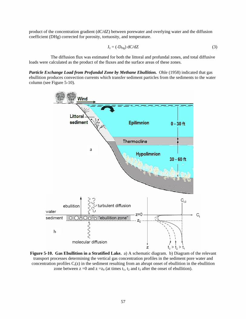
57

product of the concentration gradient (dC/dZ) between porewater and overlying water and the diffusion coefficient (DHg) corrected for porosity, tortuosity, and temperature. Jz = (-DHg) dC/dZ (3) The diffusion flux was estimated for both the littoral and profundal zones, and total diffusive loads were calculated as the product of the fluxes and the surface areas of these zones. Particle Exchange Load from Profundal Zone by Methane Ebullition. Ohle (1958) indicated that gas ebullition produces convection currents which transfer sediment particles from the sediments to the water column (see Figure 5-10).

Figure 5-10. Gas Ebullition in a Stratified Lake. a) A schematic diagram. b) Diagram of the relevant

transport processes determining the vertical gas concentration profiles in the sediment pore water and concentration profiles Ci(z) in the sediment resulting from an abrupt onset of ebullition in the ebullition

zone between z =0 and z =z0 (at times t1, t2 and t3 after the onset of ebullition).

a

b

58

Gbondo-Tugbawa et al. (2005) estimated the HgT sediment transfer load via ebullition currents of methane gas for the profundal sediments by multiplying the rate of bubble-entrained sediment transfer by the average surface sediment HgT concentration in the profundal zone. Potential Advective Load from Wind-Induced Sediment Resuspension. The HgT concentrations in the southern deep basin and on the north shore were about 5 ng/L under calm, low-turbidity condition. The water overlying the ILWD contained an average of about 10 ng/L of HgT under calm conditions. Under conditions of winds from the northwest, concentrations of HgT continued to be about 5 ng/L in the southern deep basin and on the north shore. However, the concentrations in the water overlying the ILWD doubled to an average of 20 ng/L, with the highest concentration reaching 49 ng/L. The ambient turbidity for this site was 2.1 NTUs, and the critical NW wind speed required to induce resuspension was approximately 2.2 m/s. A turbidity value of 2.1 NTUs corresponds to a TSS value of 3.3 mg/L, the ambient concentration for this area not subject to settling. The analysis conducted by Gbondo-Tugbawa et al. (2005) suggests that the frequency of critical NW winds required to cause resuspension events is approximately 35%. Over the stratified period of 121 days (based on data from 1992), the total load of HgT contributed by wind-induced resuspension on sediments from the ILWD was estimated as 6,300 g. This estimated internal load exceeds the load of about 3,400 g contributed by external sources of HgT to the lake during the 1992 stratified period. Diffusion Load from Porewater. The diffusion rates were calculated based on porewater data from the 0 to 4 cm (dZ = 2 cm) interval and overlying water concentrations assumed to be zero for an upper-bound estimate. Rates of HgT diffusion from porewater to the water column for littoral and profundal zones averaged 149 and 45 ng/m2-day, and the total diffusive load during the stratified period was 115 g. The diffusive flux estimated for littoral sediments was considered to be more representative than the hypolimnetic flux, since in situ production may be minimal in the littoral zone, as opposed to the hypolimnetic diffusive flux. The sediment concentrations measured in the upper 4 cm of the profundal cores did not represent an equilibrium concentration, but, rather, a measure of the balance between in situ production of dissolved-phase mercury and diffusional transport at the time of sampling. The magnitude of the profundal sediment flux to the hypolimnion was strongly dependent on the location of the dissolved-phase mercury production layer in the sediment. Particle Exchange Load from Profundal Zone by Methane Ebullition. The profundal sediments of Onondaga Lake produce methane gas, which bubbles out of the sediments (ebullition) at an average rate of 6 mmol/m2-day (Addess, 1990) during summer months. Using the average entrained particle transfer flux reported for a similar rate of gas ebullition at the St. Louis River/Interlake/Duluth Tar Site in Minnesota, of approximately 0.092 g/m2-day (Service Environmental & Engineering, 2002) and average surface (0 to 30 cm) sediment mercury concentration in the profundal zone about 10 mg/kg (TAMS, 2002) to Onondaga Lake, the particle transfer load calculated to be 880 g of HgT to the hypolimnetic water column during the stratified period. However, as ebullition of methane gas can significantly increase the diffusion of dissolved-phase constituents due to increased surface area and/or an increase in the contact between the overlying water and deeper sediments (Klump and Martens, 1981), this effect can further increase the diffusional load of HgT from the profundal zone. 5.19 Summary Analysis of HgT loads from internal sources including wind-induced resuspension, diffusion of dissolved-phase HgT, and particle exchange, indicate that internal sources (more than 7,000 g) contributed more than the loads estimated in the stratified period from external sources (approximately 3,400 g). During the stratified period, HgT accumulated in the hypolimnion and the profundal sediments. The water column accumulation of dissolved HgT from the sediments of the hypolimnion seems to be a

59

significant source of inorganic mercury to in-lake methylation. Under the anoxic conditions typical for Onondaga Lake during the stratified period, methylation appears to provide a major source of methylmercury to the lake where it is available for uptake and accumulation in fish and other biota. 5.20 Case Study 3. Remediation and Monitoring of Mercury Contaminated

Sediments in Lake Turingen, Sweden Mercury contaminated bottom sediments in Lake Turingen, Sweden were remediated during the Lake Turingen Remedial Project with three stages of dredging, geotextile, sand/gravel capping and artificial sediment (aluminum hydroxide) capping. It would have taken significant technical and financial resources to dredge the entire lake. During 1999–2000, a 4 ha area containing about 40% of the mercury found in the lake was partially dredged and then capped by a relatively conventional geotextile/sand cap. About 80% of the remaining contaminated lake bottoms were capped during 2002–2003 by artificial sediment based on aluminum hydroxide. It was claimed that this remediation methods have successfully inhibited resuspension of contaminated particles and led to lower concentrations of mercury in lake water. 5.21 Background Information Bottom sediments in Lake Turingen (Figure 5-11), a freshwater lake about 40 km southwest of Stockholm, Sweden, reported to be contaminated with mercury discharged between 1946 and 1966 from a paper mill.

Figure 5-11. Location of Lake Turingen, Sweden (Bergman and Petsonk, 1997)

The concentrations of mercury in contaminated sediments at various areas of the lake are shown in Figure 5-12.

60

Figure 5-12. Sediment and Mercury Loading of Contaminated Sediments in Various Areas of Lake Turingen (Bergman et al., 2005)

Aquatic life in the lake had been seriously affected by this release. Although there are large annual variations, mercury levels in pike (Esox lucius) have been more or less constant at about 2 mg/kg wet weight (w/w) since the late 1960’s (Figure 5-13).

Figure 5-13. Mercury Concentrations in Pike from Lake Turingen (Bergman et al., 2005)

61

Remedial activities were initiated in the middle of the 1990’s under the initial financial support from the Swedish Environmental Protection Agency. The remediation activities were carried out in three stages:

(a) Construction of new stream channels to isolate approximately 100 kg of mercury contaminated sediments located in two reservoirs upstream of the lake (1995),

(b) Capping in situ with a geotextile and sand/gravel of a 4-hectare large area of lake sediments outside the mouth of the stream feeding the lake, which isolated another 100 kg of mercury (1999–2000), and

(c) Capping in situ with artificial sediment of nearly 80 hectares of lake sediments found on accumulation and transport bottoms that contained most of the remaining 125 kg of mercury (2002–2003). Subsequent to these activities a five-year long monitoring program is being used to follow up the project.

5.22 Remedial Technologies The goals of this project was (a) to isolate at least 95% of all contamination in order to reduce mercury concentrations in pike and other fish species to acceptable levels, i.e. <0.5 mg/kg (w/w) as per Swedish Environmental Protection Agency’s standard, (b) to stimulate biodiversity in the watershed, and (c) to improve suitability of the lake for recreational purposes, especially fishing. After an extensive suite of remedial investigations (RI) and feasibility studies (FS), Bergman and Petsonk (1997) reported a preliminary strategy for remediation of Lake Turingen entailing removal of approx. 45,000 m3 of sediment from an area outside the mouth of the stream feeding the lake, underwater disposal of spoils in a deep part of the lake, and capping of the deposit and the rest of the lake with artificial sediment. The RI/FS concluded that spread and transport of mercury in the lake was dominated by resuspension of mercury-contaminated particles, in particular, sediments from the small (4 ha) area just outside the mouth of the stream (Meili 1998). Sediment mapping by various studies (Huononen, 1992; Hjort, 1996; and Persson, 1996) had reported that 20% of the total volume of contaminated sediments and 40% of available mercury were located in this area, in deposits of up to 3 m in depth. However, the lake of 100 ha size and low density of most sediment materials reasoned that dredging or capping with conventional materials may not be the practical or economical for more than a small part of the lake. Minimization of the amount of dredging was considered because of following reasons: a) the possible release of contaminated particles during dredging, and b) the probability that dredged areas might still have to be capped to attain performance goals. Instead, conventional capping of the area near the mouth of the stream was introduced into the remedial scenario. 5.23 Conventional Dredging and Capping Remediation of the area outside the mouth of the stream started in August 1999. To minimize the spread of contaminated material, all work was carried out within the confines of geotextile silt screens extending from the water surface to the bottom of the water column. Shallow areas overgrown with reeds were cleared and in some cases deepened. Thereafter, the lower reaches of the stream and a channel outside the mouth of the stream were dredged using the bucket dredgers. These actions were taken for the following reasons (Petersson, 1998):

• To reduce continued deposition of sediments in the southern end of the lake,

62

• To minimize the risk for flooding of land above the stream mouth during high water episodes, and

• To reduce the probability of erosion by decreasing water velocities and directing stream flow towards deeper water.

The dredged and undredged areas and the deposit were covered by a multi-layer cap (geotextile, fine sand and gravel) (see Figure 5-14).

Figure 5-14. Schematic Sectional Diagram through the Affected Area (Bergman et al., 2005) Though the dredging operations were conducted as per the expectations of project management, underwater capping proved more complicated than expected due to uneven capping, mixing of layers caused by the methodology and equipment selected for underwater placement of granular materials. 5.24 Capping with Artificial Sediment The capping technique, the Cover method (invented by Vattenresurs AB), selected for the rest of the lake used artificial sediment created by in situ precipitation of aluminum hydroxide. In order to improve material characteristics, it was augmented with inert ballast and reinforcing materials (Carlsson, 1996; Carlsson and Eriksson, 1998). Capping materials and techniques were evaluated using laboratory tests of physical and chemical characteristics, and field tests of cap placement. A pilot-scale version of the equipment was used to place the artificial sediment in a test plot on the bottom of the lake. A laboratory study (Meili and Skarp, 2002) reported that during a test period of 218 days, significant amounts of mercury did not diffuse through the cap. It was also reported that larvae of Chironomus plumosus introduced onto the cap apparently thrived in that environment, which indicated that bioturbation could be an important factor with regard to transport of mercury from underlying materials through an artificial sediment cap. Persson (1996) estimated the depth of bioturbation to be approximately two to three centimeters, an average cap thickness of four centimeters was selected. A greater thickness (up to 6 cm) was selected in areas with higher mercury concentrations and a larger exposure to erosional forces (transport bottoms), while a lesser thickness (3 cm) was allowed in areas with lower contaminant levels and/or less risk of erosion and bioturbation, i.e. deep accumulation bottoms.

63

An analytical technique (Kaj and Skarp, 1997) based on leaching of aluminum at pH 4 followed by standard analysis (e.g. AAS or ICP) was used for differentiating artificial sediment from natural sediment. The artificial sediment was created by reacting aluminum chloride (AlCl3), caustic (NaOH), inert ballast, and reinforcing materials as per chemical reaction below:

AlCl3 + 3 NaOH + additives → Al(OH)3 + 3Na+ + 3Cl-

5.25 Construction Quality Control (CQC) and Environmental Monitoring (EM) Construction quality control (CQC) and environmental monitoring (EM) were conducted to oversee remediation of mercury contaminated bottom sediments and to provide project management with indications of the short and long-term effects of remedial activities and conformance with specifications. Visual monitoring, measurement of turbidity, divers and underwater video were the primary CQC-tools during one stage of the project (1999–2000), when 4 ha were capped using a conventional geotextile and sand. In a later stage (2002–2003), core sampling, sediment traps and underwater video were used to monitor the 80 ha capped with artificial sediment. The EM-program encompasses regular sampling of lake and river water, falling sediment and biological matrices. Stage B. The dredging and capping with a conventional multi-layer cap were major components of Stage B remediation. Geotextile silt screens were extended from the water surface and were anchored in lake bottom sediments. During construction, the CQC-tools were visual monitoring and measurement of turbidity within, between and outside the screens. Inspections of cap were made upon completion of construction work using divers who walked across the cap probing the various layers, and by use of an underwater video camera mounted on a specially designed sled, the was inspected to ascertain conformity. Settlement and lateral movement of the unconsolidated sediments caused by the heavy capping materials were monitored by measurement stations. The measurement stations are in place for three years after completion of the construction work. Stage C. Stage C remediation was conducted using capping with artificial sediment based on Al(OH)3. The artificial sediment was produced in-situ by reacting AlCl3 and NaOH. Sediment production was monitored using visual inspection of cores (Figure 5-15), specially designed bucket sediment traps, underwater video, and by measurements of water quality. Such inspections were carried out both in test areas prior to the start of full-scale production as well as during and after placement of artificial sediment.

Figure 5-15. Core sample after treatment. Artificial Sediment is the Light-

Colored Material (Petsonk et al., 2005)

64

The EM-program, including the measurements/sampling at various stations to monitor various media and environmental parameters, is scheduled to continue to 2008. A variety of biota was included in the program in order to provide a range of short-, medium- and long-term biological responses (Table 5-4).

Table 5-4. Monitoring Media, Parameters, and Frequency for Environmental Monitoring (after Petsonk et al., 2005)

Medium Parameter Measurement Frequency

Noise (i) Background noise (ii) Construction noise

As required

Meteorological data (i) Air temperature (ii) Precipitation (iii) Wind speed and direction

Every 15 minutes

Hydrological data (i) Lake water levels (ii) Stream flow

At least quarterly; weekly or daily during Stage B

Lake and stream water (i) pH, alkalinity, color (ii) Turbidity, visibility (iii) Al, Cl, Fe, Mn, Hg, methyl-

Hg (iv) Temperature, O2, EC, redox

At least quarterly; weekly or daily during Stage B

Falling sediment (i) Al, pH4-Al(1), Fe, Mn, Hg, TOC

(ii) Sedimentation rate

At 8 - 12 week intervals

Bottom sediment Al, pH4-Al(1), Fe, Mn, Hg, N, P, TOC

As required

Zooplankton (i) Hg, methyl-Hg (ii) Species

At least quarterly; weekly or daily during Stage B

Benthic and littoral fauna (i) Species (ii) Hg, methyl-Hg

Annually

Perch, pike (i) Weight, length, sex, age (ii) Hg, methyl-Hg

Annually

pH4-Al = Unpublished analytical technique developed by Swedish Scientists (L. Kaj and J. Skarp) to measure leachability of aluminum at pH 4.

5.26 Results Environmental monitoring of water, falling sediment, bottom sediment, zooplankton, macro-benthic fauna and fish was conducted after the remedial activities (Bergman and Carlsson, 2005). The major observations are summarized below:

• Total mercury concentrations in stream water feeding the lake decreased following the Stage A remediation (isolation of upstream reservoir sediments).

65

• Elevated levels during the late 1990’s and early 2000’s probably reflect the continued erosion of smaller pockets of residual contamination along the streambed during high-flow periods.

• Follow-up monitoring of the conventional cap indicates that there has been a substantial amount of subsidence and compaction of underlying sediment and some lateral movement. Bergman and Carlsson (2005) reported that these movements have actually improved the quality of the cap, as capping materials are more evenly distributed and therefore more effective as a new lake bottom. The cap allows passage of gas generated by degradation of underlying materials, but does not permit release of measurable amounts of mercury.

• Visual monitoring clearly demonstrated that the silt screens successfully limited the spread of suspended matter from dredging and capping operations. Turbidity measurements were also performed at a variety of stations on a more or less daily basis while operations were ongoing to ensure that such materials did not leak through or around the screens. Monitoring results confirmed the effectiveness of the screens and at one point led to the discovery of a hole chewed through the geotextile by a visitor from a colony of beavers. Underwater inspections using divers noted a number of deficiencies, including bubbles where capping materials were missing or insufficient, locations where those materials were placed in an incorrect sequence, and a generally large degree of unevenness. Monitoring of settlement and lateral movement in the sediments showed that the rates of movement at two of three measurement stations became very small after the first two years, while there was still apparently quite a bit of movement even after three years at the third station.

Monitoring of falling sediment (Figure 5-16) has been performed since 1994 at four of the stations, two in the lake itself (SN and C) and two downstream (L and M). The 1995 works (Stage A) had very little effect on falling sediment. However, capping outside the mouth of the stream (Stage B) brought about significant reductions of both sediment flux and mercury levels. This confirmed that resuspension of sediment from that area was a dominant source of falling sediment in the rest of the lake, and indicated that the most important source of mercury-contaminated particulate had probably been eliminated. The data from 2003–2004 seem to show additional reductions due to the capping with artificial sediment (Stage C). The high sediment flux at stations SN and C during 2002–2003 reflect the production of artificial sediment.

Figure 5-16. Yearly Minimum and Maximum Sediment Loadings and Mercury

Concentrations in Falling Sediment 0.5 – 1 m Above Lake Bottom (Bergman et al., 2005)

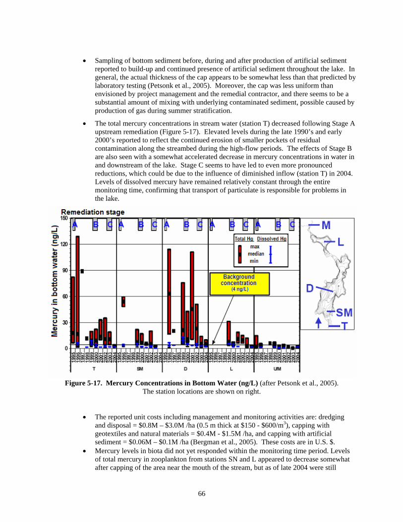
66

• Sampling of bottom sediment before, during and after production of artificial sediment

reported to build-up and continued presence of artificial sediment throughout the lake. In general, the actual thickness of the cap appears to be somewhat less than that predicted by laboratory testing (Petsonk et al., 2005). Moreover, the cap was less uniform than envisioned by project management and the remedial contractor, and there seems to be a substantial amount of mixing with underlying contaminated sediment, possible caused by production of gas during summer stratification.

• The total mercury concentrations in stream water (station T) decreased following Stage A upstream remediation (Figure 5-17). Elevated levels during the late 1990’s and early 2000’s reported to reflect the continued erosion of smaller pockets of residual contamination along the streambed during the high-flow periods. The effects of Stage B are also seen with a somewhat accelerated decrease in mercury concentrations in water in and downstream of the lake. Stage C seems to have led to even more pronounced reductions, which could be due to the influence of diminished inflow (station T) in 2004. Levels of dissolved mercury have remained relatively constant through the entire monitoring time, confirming that transport of particulate is responsible for problems in the lake.

Figure 5-17. Mercury Concentrations in Bottom Water (ng/L) (after Petsonk et al., 2005). The station locations are shown on right.

• The reported unit costs including management and monitoring activities are: dredging and disposal = $0.8M – $3.0M /ha (0.5 m thick at $150 - $600/m3), capping with geotextiles and natural materials = $0.4M - $1.5M /ha, and capping with artificial sediment = $0.06M – $0.1M /ha (Bergman et al., 2005). These costs are in U.S. $.

• Mercury levels in biota did not yet responded within the monitoring time period. Levels of total mercury in zooplankton from stations SN and L appeared to decrease somewhat after capping of the area near the mouth of the stream, but as of late 2004 were still

67

elevated far above reference levels. Levels of methyl mercury in zooplankton, which usually constitute 60–80% of total mercury concentrations, follow a similar pattern.

• Mercury concentrations in macro-benthic fauna, perch and pike did not shown any significant influence from the remedial activities within the monitoring period.

• It should be noted that caution must be applied to interpretation of data, as the amount of data is still relatively small during the short length of the study to confirm trends.

68

Section 6.0: REFERENCES Abreu, S.N., Pereira, M.E., and A.C. Duarte. 1998. The use of a mathematical model to evaluate

mercury accumulation in sediments and recovery time in a coastal lagoon (Ria De Aveiro, Portugal). Water Science and Technology 37(6-7):33-38.

Adams, D.D. Fendinger, N.J. and Glotfelty, D.E. 1997. Biogenic gas production and mobilization of in-place sediment contaminants by gas ebullition. In: Sediments: Chemistry and Toxicity of In-Place Pollutants. R Baudo, J Geisy and H Muntau (Eds.), Lewis Publishers, Boca Raton, FL.

Addess, J.M. 1990. Methane Cycling in Onondaga Lake, NY. Master’s Thesis, College of Environmental Science and Forestry, State University of New York. Syracuse, NY.

Alberts, J.J., Schindler, J.E., Miller, R.W. and D.E. Nutter. 1974. Elemental mercury evolution mediated by humic acid. Science 184:895–897.

Alcoa, 1996. Mercury Reconnaissance Study, Remedial Investigation Work Plan, Volume B2C: Data Report

Alcoa, 1998. Sediment Transport Study: Radiochemistry Study, Remedial Investigation Work plan: Volume B3.

Alcoa, 1999. Remedial Investigation Report.

Alcoa, 2000. Treatability Dredge Study for Alcoa (Point Comfort)/ Lavaca Bay Superfund Site.

Alcoa, 2001. Feasibility Study for Lavaca Bay Superfund Site.

Alcoa, 2003. Remedial Design Reports on (1) Chlor Alkali Process Area: Groundwater, Chlor Alkali Process Area: Soil, (2) Chlor Alkali Process Area: Groundwater, (3) Witco Area: soil, (4) Witco Area: Marshes, (5) DNAPL Containment System, (6) North of Dredge Island Enhanced Natural Recovery, and (7) Lavaca Bay Sediments and Long-Term Management.

Amirbahman, A., Reid, A.L., Haines, T.A., Kahl, J.S. and C. Arnold. 2002. Association of methylmercury with dissolved humic acids. Environ. Sci. Technol. 36:690–695.

Amyot, M., Gill, G.A., and F.M.M. Morel. 1997. Production and loss of dissolved gaseous mercury in the coastal seawater. Environmental Science and Technology 31:3606-3611.

Andren, A.W., and R.C. Harriss. 1975. Observation on the association between mercury and organic matter dissolved in natural waters, Geochim. Cosmochim. Acta 39:1253-1257.

AWWA. 2001. Water Resource Planning Manual (M50). W.O. Maddaus (Ed.) American Water Works Association, AWWA, Denver, CO.

Azcue, J.M., Zeman, A.J., Mudroch, A., Rosa, F., and T. Patterson. 1998. Assessment of sediment and porewater after one year of subaqueous capping of contaminated sediments in Hamilton Harbour, Canada. Water Science Technology 37(6-7):323-329.

Babel, S. and T.A. Kurniawan. 2003. Low-cost adsorbents for heavy metals uptake from contaminated water: a review. Journal of Hazardous Materials 97(1-3):219-243.

Babiarz, C.L., Hurley, J.P., Hoffmann, S.R., Andren, A.W., Shafer, M.M., and D.E. Armstrong. 2001. Partitioning of total mercury and methylmercury to the colloidal phase in freshwaters. Environ. Sci. Technol. 35(24):4773-4782.

69

Bale, A.E. 2000. Modeling aquatic mercury fate in Clear Lake, California. Journal of Environmental Engineering 126(2): 153-163.

Barbosa, M.C. and M.d.S. Soares de Almeida. 2001. Dredging and disposal of fine sediments in the state of Rio de Janeiro, Brazil. Journal of Hazardous Materials 85:15-38.

Barkay, T., Gillman, M. and R.R. Turner. 1997. Effects of dissolved organic carbon and salinity on bioavailability of mercury. Appl. Environ. Microbiol. 63:4267–4271.

Battelle. 1987. Measurement of bioavailable mercury species in fresh water and sediments. Electric Power Research Institute, Palo Alto, California.

Baumgarten G., 2001. RPM Panel Discussion: Sediment Remediation. Presented at the Technical Support Project Meeting. http://www.epa.gov/tio/tsp/download/baumgarten-rpmpanel.pdf

Beijer, K. and A. Jernelov. 1979. Methylation of mercury in aquatic environments. In: The Biogeochemistry of Mercury in the Environment. J. O. Nriagu (Ed.), pp. 203-210. Elsevier/North-Holland Biomedical Press, New York

Ben-Jemaa, F., Mariño, M.A. and A. Hugo. 1995. Loaiciga Sampling Design for Contaminant Distribution in Lake Sediments. J. Water Resour. Plng. and Mgmt. 121(1):71-79.

Benoit J.M., Mason, R.P., Gilmour, and C.C. 1999. Estimation of mercurysulfide speciation in sediment pore waters using octanol–water partitioning and implications for availability to methylating bacteria. Environ. Toxicol. Chem. 18:2138–2141.

Benoit, J.M., Gilmour, C.C., Mason, R.P., and A. Heyes. 1999. Environ Sci. Technol. 33:951-957.

Bergman, R. and A.M. Petsonk. 1997. Lake Turingen Remedial Project: Isolation of Mercury Contaminated Sediments. Proc. Intl. Conference on Contaminated Sediments, Rotterdam. pp 25-32.

Bergman, R., Carlsson, S-Å, and A.M. Petsonk. 2005. In-Situ Mitigation of Mercury Contaminated Sediments in Lake Turingen. Intl. Conference on Remediation of Contaminated Sediments, New Orleans.

Blazquez, C.A., Adams, T.M., and P. Keillor. 2001. Optimization of mechanical dredging operations for sediment remediation. Journal of Waterway, Port, Coastal, and Ocean Engineering 127:299-307.

Bloom, N. S., Gill, G. A., Cappellino, S., Mschea, L. Dobbs, C. Driscoll, C., Mason, R., and J. Rudd. 1999. Speciation and Cycling of Mercury in Lavaca Bay, Texas, Sediments, Environ. Sci. Technol., 33:7-13.

Bloom, N.S. and E.A. Crecelius. 1983. Determination of mercury in seawater at subnanogram per litre levels. Marine Chemistry 14:49-59.

Bloom, N.S. and S.W. Effler. 1990. Seasonal variability in the mercury speciation of Onondaga Lake (New York). Water, Air, Soil Pollut. 53:251-265.

Bloom, N.S., Watras, C.J. and J.P. Hurley. 1989. Impact of acidification on the methylmercury cycle of remote seepage lakes. Water, Air, and Soil Poll. 56:477-491.

Bloom, N.S. and B.K. Loasorsa, B.K. 1999. Changes in mercury speciation and the release of methyl mercury as a result of marine sediment dredging activities. The Science of the Total Environment 237/238:379-385.

70

Braga, M.C.B., Shaw, G., Lester, J.N. 2000. Mercury modeling to predict contamination and bioaccumulation in aquatic ecosystems. In: Reviews of environmental contamination and toxicology, G.W. Ware (Ed.) Springer, New York. 164:69–92.

Budinova, T., Savova, D., Petrov, N., Razvigorova, M., Minkova, V., Ciliz, N., Apak, E. and E. Ekinci. 2003. Mercury Adsorption by Different Modifications of Furfural Adsorbent. Ind. Eng. Chem. Res., 42 (10):2223 -2229.

Buffle, J. 1988. Complexation Reactions in Aquatic Systems. Ellis Horwood Ltd., Chichester.

Callister, S.M. and Winfrey, M.R. 1986. Microbial methylation of mercury in upper Wisconsin River sediments. Water, Air and Soil Pollution 29:453-465.

Carroll, R.W.H., Warwick, J.J., Heim, K.J., Bonzongo, J.C., Miller, J.R., and W.B. Lyons. 2000. Simulation of mercury transport and fate in the Carson River, Nevada. Ecological Modelling 125:255-278.

Charlet, L., Bosbach, D., and T. Peretyashko. 2002. Natural attenuation of TCE, As, Hg linked to the heterogeneous oxidation of Fe(II): an AFM study. Chemical Geology 190(1-4):303-319.

Chattopadhyay, S. 2005. Grain Incident and Other Mercury Tragedies: Forms, Fate and Effects. In: Encyclopedia of Toxicology. P. Wexler (Editor in Chief), Elsevier, Oxford, UK.

Chau, Y.K., Snodgrass, W.J. and P.T.S. Wong. 1977. A sampler for collecting evolved gases from sediment. Water Research 11: 807-809.

Chojnackia, A., Chojnacka, K., Hoffmanna, J. and H. Góreckia. 2004. The application of natural zeolites for mercury removal: from laboratory tests to industrial scale. Minerals Engineering 17(7-8):933-937.

Cleam, V., and D. S. Gamble. 1974. Metal-fulvic acid chelation equilibrium in aqueous NaNO3 solutions: Hg(II), Cd(II), and Cu(II) fulvate complexes. Can J. Soil Sci. 54:413-417.

Cleckner, L.B., Gilmour, C.C., Hurley, J.P., and D.P. Krabbenhoft. 1999. Mercury methylation in periphyton of the Florida Everglades. Limnology and Oceanography 44:1815–1825.

Collins, C.R., Sherman, D.M., and K.V. Ragnarsdottir. 1999. Surface complexation of Hg2+ on goethite: Mechanism from EXAFS spectroscopy and density functional calculations. J. Colloid Interface Sci. 219:345-350.

Compeau, G. and R. Bartha. 1983. Effects of sea salt anions on the formation and stability of methylmercury. Bulletin of Environmental Contamination and Toxicology 31:486-493.

Coston, J.A., Fuller, C.C., and J.A. Davis. 1995. Pb2+ and Zn2+ adsorption by a natural aluminum-bearing and iron-bearing surface coating on an aquifer sand. Geochim. Cosmochim. Acta 59:3535-3547.

Cushing, B.S. 1999. Identification and evaluation of remedial dredging difficulties. Journal of Dredging Engineering 1:16-33.

Counter S. A.; Buchanan L. H.; Mercury Exposure in Children: A review, Science Direct, Toxicology and Applied Pharmacology, 198, 209-230, 2004.

Craig, P.J., and P.A. Moreton. 1985. The role of speciation in mercury methylation in sediments and water. Environmental Pollution Series B 10:141-158.

71

Cruz-Guzmán, M., Celis, R., Hermosín, Leone, P., Nègre, M., and J. Cornejo. 2003. Sorption-desorption of lead (II) and mercury (II) by model associations of soil colloids. Soil Sci. Soc. Am. J. 67:1378-1387.

De Diego, A., Tseng, C.M., Dimov, N., Amouroux, D., and F.X. Donard. 2001. Adsorption of aqueous inorganic mercury and methylmercury on suspended kaolin: influence of sodium chloride, fulvic acid and particle content. Applied Organometallic Chemistry 15:490–498.

Degetto, S., Schintu, M., Contu, A., Sbrignadello, G. 1997. Santa Gilla lagoon (Italy): A Mercury Sediment Pollution Case Study. Contamination assessment and restoration of the site. Sci. Total Environ. 204:49–56.

Diamond, M.L. 1999. Development of a fugacity/equivalence model of mercury dynamics in lakes. Water, Air, and Soil Pollution 111:337-357.

Doktycz, S.J., and Suslick, K.S. 1990. Interparticle collisions driven by ultrasound. Science, 247:1067-1039.

Drexel, R.T., Haitzer, M., Ryan, J.N., Aiken, G.R. and K.L. Nagy. 2002. Mercury (II) sorption to two Florida Everglades peats: evidence for strong and weak binding and competition by dissolved organic matter released from the peat. Environ. Sci. Technol. 36:4058–4064.

Driscoll, C.T., Blette, V., Yan, C., Schofield, C.L., Munson, R. and J. Holsapple. 1995. The role of dissolved organic carbon in the chemistry and bioavailability of mercury in remote Adirondack lakes. Water, Air, Soil Pollut. 80:499–508.

Dyrssen, D. and Wedborg, M. 1991. The sulfur-mercury (II) system in natural waters. Water Air Soil Poll. 56:507-519.

Effler, S. W. and M. G. Perkins. 1996. Optics. In: Limnological and Engineering Analysis of a Polluted Urban Lake, Prelude to Environmental Management of Onondaga Lake, New York. S. W. Effler (Ed) pp. 535-599. Springer-Verlag, New York, NY.

Ehrhardt, J.J., Behra, P., Bonnissel-Gissinger, P., and M. Alnot. 2000. XPS study of the sorption of Hg(II) onto pyrite FeS2. Surf. Interface Anal. 30:269-272.

Falter, R. 1999. Experimental study on the unintentional abiotic methylation of inorganic mercury during analysis: Part 1: Localisation of the compounds effecting the abiotic mercury methylation. Chemosphere 39(7):1051-1073.

Fendinger, N.J. 1981. Distribution and related fluxes of dissolved pore water gases in sediments of Lake Erie and two polluted harbors. M. S. Thesis, Wright State University, Dayton, OH.

Fitzgerald, W.F.,Vandal, G.M., Mason, R.P., and F. Dulac. 1994. Air-water cycling of mercury in lakes. In Mercury Pollution—Integration and Synthesis, C.J. Watras and J.W. Huckabee (Eds.), 203–220, CRC Press, Boca Raton, FL.

Gagnon, C. and N.S. Fisher. 1997. Bioavailability of sediment bound methyl and inorganic mercury to a marine bivalve. Environ. Sci. Technol. 31:993– 998.

Gao, Y., Kan, A.T., Tomson, M.B. 2003. Critical evaluation of desorption phenomena of heavy metals from natural sediments. Environ. Sci. Technol. 37:5566-5573.

Garbaciak, S., Spadaro, P., Thornburg, T., and R. Fox. 1998. Sequential risk mitigation and the role of natural recovery in contaminated sediment projects. Water Science and Technology 37(6-7),331-336.

72

Gbondo-Tugbawa, S., and C.T. Driscoll, C.T. 1998. Application of the regional mercury cycling model (RMCM) to predict the fate and remediation of mercury in Onondaga Lake, New York. Water, Air, and Soil Pollution 105:417-426.

Gbondo-Tugbawa, S.S., Garvey, E., Montione, R., and M.L. Spera. 2005 Dynamics of Mercury in Onondaga Lake, New York. Proceedings of the Third International Conference on Remediation of Contaminated Sediments. New Orleans, LA.

Gill, G. A.; Bloom, N. S; Cappellino, S.; Mschea L. and Dobbs C.; Driscoll, C.; Mason, R.; Rudd J.; Sediment-Water Fluxes of Mercury in Lavaca Bay, Texas, Environ. Sci. Technol., 33, 663-669, 1999.

Gill, G.A. and K.W. Bruland. 1990. Mercury speciation in surface freshwater systems in California and other areas. Environ. Sci. Technol. 24(9):1392-1400.

Gill, G.A. and W.F. Fitzgerald. 1987. Picomolar mercury measurements in seawater and other materials using stannous chloride reduction and two-stage gold amalgamation with gas phase detection. Marine Chemistry 20:227-243.

Gilmour, C. C., Henry, E. A., and R. Mitchell. 1992. Sulfate stimulation of mercury methylation in freshwater sediments. Environ. Sci. Technol. 26:2281-2287.

Gilmour, C.C. and E.A. Henry. 1991. Mercury methylation in aquatic systems affected by acid deposition. Environmental Pollution 71(2-4): 131-169.

Glass, G.E., Sorensen, J.A., Schmidt, K.W. and G.R. Rapp. 1990. New source identification of mercury contamination in the Great Lakes. Environ. Sci. Technol. 24(7):1059-1069.

Guentzel, J.L., Powell, R.T., Landing, W.M. and R.P. Mason. 1996. Mar. Chem. 55:177-188.

Guo, L.D., Hunt, B.J., Santschi, P.H., and S.M. Ray. 2001. Environ. Sci. Technol. 35:885-893.

Haitzer, M., Aiken, G.R. and J.N. Ryan. 2002. Binding of mercury (II) to dissolved organic matter: the role of the mercury-to-DOM concentration ratio. Environ. Sci. Technol. 36:3564–3570.

Halbach, S. 1995. Toxicity of detrimental metal ions. In: Handbook of Metal–Ligand Interactions in Biological Fluids––Bioinorganic Medicine. G. Berthon (Ed.). vol. 2, pp. 749–754. Marcel Dekker, Basel.

Hamblin, P.F., Zhu, D.Z., Chiocchio, F., He, C., and M.N. Charlton. 2000. Monitoring suspended sediment plumes by optical and acoustical methods with application to sand capping. Canadian Journal of Civil Engineering 27:125-137.

Hasterberg, D., Chou, J.W., Hutchison, J.K. and D.E. Sayers. 2001. Bonding of Hg(II) to reduced organic sulfur in humic acid as affected by S/Hg ratio. Environ. Sci. Technol. 35:2741–2745.

He, Z., Traina, S.J., Bigham, J.M., and L.K. Weavers. 2005. Sonolytic desorption of mercury from aluminum oxide. Environ. Sci. Technol. 39(4):1037-1044.

Henry, E.A., Dodge-Murphy, L.J., Bigham, G.N., and S.M. Klein. 1995. Modeling the transport and fate of mercury in an urban lake (Onondaga Lake, NY). Water, Air, and Soil Pollution 80:489-498.

Heslein, R.H. 1976. The fluxes of methane, carbon dioxide and ammonia from sediments and their consequent distribution in a small lake, PhD dissertation, Columbia University, NY.

Hessen, D.O., Andersen, T., A. Lyche. 1990. Limnol. Oceanogr. 35:84-99.

73

Hintelmann, H., Ebinghaus, R., and R-D. Wilken. 1993. Accumulation of mercury(II) and methylmercury by microbial biofilms. Water Research 27:237–242.

Hintelmann, H. and R. Harris. 2004. Application of multiple stable mercury isotopes to determine the adsorption and desorption dynamics of Hg(II) and MeHg to sediments Marine Chemistry 90(1-4):165-173.

Holmer, M. and P. Storkholm. 2001. Sulphate reduction and sulphur cycling in lake sediments: a review. Freshwater Biology 46:431-451.

Hosokawa, Y. 1993. Remediation work for mercury contaminated bay - experiences of Minamata Bay Project, Japan. Water Science and Technology 28 (8-9), 339-348.

Howard D.L., Frea J.I. and R.M. Pfister. 1971. The potential for methane-carbon cycling in Lake Erie In Proc. 14th Conf. Int. Assoc. Great Lakes Research, Ann Arbor Press, MI.

Hudson, R.J.M., Gherini, S.A., Watras, C.J., and D.B. Porcella. 1994. Modeling the biogeochemical cycle of mercury in lakes. In: Mercury pollution: Integration and synthesis, C.J. Watras and J.W. Huckabee (Eds.), Lewis, Boca Raton, FL., pp. 473–523.

Hurley, J.P., Watras, C.J., and N.S. Bloom. 1991. Mercury cycling in a northern seepage lake: the role of particulate matter in vertical transport. Water Air Soil Pollut. 56:543–551.

Hurley, J.P., Krabbenhoft, D.P., Babiarz, C.L. and A.W. Andren. 1994. Cycling of mercury across sediment–water interface in seepage lakes. In: Environmental Chemistry of Lakes and Reservoirs, L.A. Baker (Ed.), pp. 425–449. American Chemical Society, Washington, DC.

Hurley, J.P., Krabbenhoft, D.P., Cleckner, L.B., Olson, M.L., Aiken, G.R. and P.S. Rawlik. 1998. System controls on the aqueous distribution of mercury in the northern Florida Everglades. Biogeochemistry 40:293–311.

Hydroqual. 1998 Hurricane Scour Model Report: Development and application of a modeling framework to evaluate hurricane impacts on surficial mercury concentrations in Lavaca bay; Copy to Alcoa.

Hylander, L.D., Pinto, F.N., Guimaraes, J.R.D., Meili, M., Oliveira, L.J., Silva, E.D.E. 2000. Fish mercury concentration in the Alto Pantanal, Brazil: influence of season and water parameters. Sci. Total Environ. 261:9–20.

Jacobs, P.H. and U. Forstner. 1999. Concept of subaqueous capping of contaminated sediments with active barrier systems (ABS) using natural and modified zeolites. Water Research 33: 2083-2087.

Jørgensen B.B. (1990) The sulfur cycle of freshwater sediments: Role of thiosulfate. Limnology and Oceanography 35:1329-1342.

Johnson, B.D., Boudreau, B.P., Gardiner, B.S. and R. Maass. 2002. Mechanical response of sediments to bubble growth, Marine Geology 187:347–363.

Jones, C. and J. Roberts. 2005. Evaluating Sediment Transport: Evaluating Sediment Transport: Tools, Techniques, and Applications Tools, Techniques, and Applications to Site Management. Conference on Remediation of Contaminated Sediments, New Orleans, LA.

Kalin, L. and M.M. Hantush. Evaluation of Sediment Transport Models and Comparative Application of Two Watershed Models. EPA Report EPA/600/R-03/139.

Kaplan, D.I., Knox, A.S., and J. Myers. 2002. Mercury geochemistry in a wetland and its implications for in-situ remediation. Scientific and Technical Information & Site Support Group of the

74

Management Services Department, Westinghouse Savannah River Site. Document WSRC-MS-2002-00056.

Karunasagar, D., Balarama Krishna, M.V., Rao, S.V. and J. Arunachalam. 2005. Removal and preconcentration of inorganic and methyl mercury from aqueous media using a sorbent prepared from the plant Coriandrum sativum. Journal of Hazardous Materials 118(1-3):133-139 .

Kasprzyk-Hordern, B. 2004. Chemistry of alumina, reactions in aqueous solution and its application in water treatment. Adv. Colloid Interface Sci. 110:19-48.

Kelly, C.A., Rudd, J.W.M., and M.H. Holoka. 2003. Effect of pH on mercury uptake by an aquatic bacterium: implications for Hg cycling. Environ. Sci. Technol. 37(13);2941-2946.

Kelly, C.A., Rudd, J.W.M., St. Louis, V.L. and A. Heyes. 1995. Is total mercury concentration a good predictor of methyl mercury concentration in aquatic systems? Water, Air, and Soil Pollution 80:715-724.

Khan, F.I. and T. Husain. 2002. Clean up contaminated sites. American Institute of Chemical Engineers. http://www.cepmagazine.org.

Kim, C.S., Rytuba, J.J., and G.E. Brown, Jr. 2003. EXAFS study of mercury(II) sorption to Fe- and Al-(hydr)oxides. II. Effects of chloride and sulfate. J. Colloids and Interface Science 270:9-20.

Kim, C.S., Rytuba, J.J., and G.E. Brown, Jr. 2004a. EXAFS study of mercury(II) sorption to Fe- and Al-(hydr)oxides. I. Effects of pH. J. Colloids and Interface Science 271:1-15.

Kim, D., Wang, Q., Sorial, G.A., Dionysiou, D.D., and D. Timberlake. 2004b. A model approach for evaluating effects of remedial actions on mercury speciation and transport in a lake system. Science of the Total Environment 327:1-15.

Klump, J. V. and C. S. Martens. 1981. Biogeochemical cycling in an organic rich coastal marine basin-II. Nutrient sediment-water exchange processes. Geochimica et Cosmochimica Acta. 45: 101-121.

Krabbenhoft, D.P. and C.L. Babiarz. 1992. The role of groundwater transport in aquatic mercury cycling. Water Resour. Res. 28:3119–3128.

Krom, M.D., Kaufman, A., and H. Hornung. 1994. Industrial mercury in combination with natural Pb210 as time-dependent tracers of sedimentation and mercury removal from Haifa Bay, Israel. Estuarine, Coastal and Shelf Science 38:625-642.

Leermakers, M., Meulemann, C., and W. Baeyens. 1995. Mercury speciation in the Scheldt estuary. Water, Air and Soil Pollution 80:641– 652.

Leppard, G., and B. Burnison. 1983. Bioavailability: Trace element associations with colloids and an emerging interest in colloidal organic fibrils. In: Trace Element Speciation in Surface Waters and Its Ecological Implications. G.G. Leppard (Ed.)1st ed., pp 105-122. Plenum Press: New York.

LeRoux, S.M., Turner, A., Millward, G.E., Ebdon, L., and P. Appriou. 2001. Partitioning of mercury onto suspended sediments in estuaries. Journal of Environmental Monitoring 3:37– 42.

Liu, C., Jay, J.A., Ika, R., Shine, J.P., and T.E. Ford. 2001. Capping efficiency for metal-contaminated marine sediment under conditions of submarine groundwater discharge. Environmental Science and Technology 35:2334-2340.

Long, E.R. and L.G. Morgan. 1991. The potential for biological effects of sediment sorbed contaminants tested in the National Status and Trends Program. U.S. National Oceanographic and Atmospheric Administration, NOAA Technical Memorandum NOS OMA 52. 175 p.

75

Loux, N.T. 1998. An assessment of mercury-species-dependent binding with natural organic carbon. Chem. Spec. Bioavail. 10:127–136.

Loux, N.T. 2005. Modeling monomethylmercury and tributyltin speciation with EPA’s geochemical speciation model MINTEQA2. Ecosystems Research Division, National Exposure Research Laboratory. EPA/600/R-05/063.

Lu, Y., Riyanto, N., and L.K. Weavers. 2002. Sonolysis of synthetic sediment particles: particle characteristics affecting particle dissolution and size reduction. Ultrason. Sonochem. 9:181-188.

Lyon, B.F., Ambrose, R., Rice, G., and C. J. Maxwell. 1997. Calculation of soil-water and benthic sediment partition coefficients for mercury. Chemosphere. 35(4):791-808.

MacDonald, D.D., C.G. Ingersoll, and T.A. Berger. 2000. Development and Evaluation of Consensus-Based Sediment Quality Guidelines for Freshwater Ecosystems. Archives of Environmental Contamination and Toxicology 39:20-31.

Macintosh, D.L., Suter, G.W., and F.O. Hoffman. 1994. Uses of Probabilistic Exposure Models in Ecological Risk Assessments of Contaminated Sites. Risk Analysis 14(4):405-419.

Marvin-Dipasquale, M., and R.S. Oremland. 1998. Bacterial methylmercury degradation in Florida everglades peat sediment. Environmental Science and Technology 32, 2556-2563.

Marvin-Dipasquale, M., Agee, J., Mcgowan, C., Oremland, R.S., Thomas, M., Krabbenhoft, D., and C.C. Gilmour. 2000. Methylmercury degradation pathways: a comparison among three mercury-impacted ecosystems. Environmental Science and Technology 34:4908-4916.

Mason R., Bloom, N., Cappellino, S., Gill, G., Benoit, J., and C. Dobbs. 1998. Investigation of Porewater Sampling Methods for Mercury and Methylmercury. Environ. Sci. Technol. 32:4031-4040.

McLaughlin, M.J. 2001. Ageing of metals in soils changes bioavailability. Fact Sheet on Environmental Risk Assessment, The International Council on Metals and the Environment, No. 4.

MDEP. 2002. Freshwater Sediment Screening Benchmarks for Use Under the Massachusetts Contingency Plan. Technical Update – May. http://www.mass.gov/dep/cleanup/laws/sedscrn.doc.

Meili, M. 1991. The coupling of mercury and organic matter in the biogeochemical cycle—Towards a mechanistic model for the boreal forest zone. Water, Air and Soil Pollution, 56:333–347.

Mierle, G. and R. Ingram. 1991. The role of humic substances in the mobilization of mercury from watersheds. Water, Air, Soil Pollut. 56:349–357.

Meili, M. 1997. Mercury in lakes and rivers. Metal Ions Biol. Syst. 34:21–51.

Meili, M., Iverfeldt, A., and L. Hakanson. 1990. Mercury in the surface water of Swedish forest lakes – concentrations, speciations, and controlling factors. Water, Air, and Soil Pollution 56:439-453.

Meriç, S., Petruzzelli, D., Iaccarino, M., and G. Pagano. 2001. Composition and toxicity of bauxite solid residues: Risk assessment and prospects for site remediation. International Symposium on Environmental Pollution and its Impact on Life in the Mediterranean Region. The Mediterranean Scientifi c Association of Environmental Protection and The Society of Ecotoxicology and Environmental Safety. Limassol, Cyprus.

Mikac, N., Niessen, S., Ouddane, B., and M. Wartel. 1999. Speciation of mercury in sediments of the Seine estuary (France). Applied Organometallic Chemistry 13:715– 725.

76

Miskimmin, B.M. 1991. Effect of natural levels of dissolved organic carbon (DOC) on methylmercury formation and sediment–water partitioning. Bull. Environ. Contam. Toxicol. 47:743–750.

Miles, C.J., Moye, H.A., Phlips, E.J., and B. Sargent. 2001. Partitioning of monomethylmercury between freshwater algae and water. Environmental Science and Technology 35:4277– 4282.

Moore, J.W. and S. Rarnamodomy. 1984. Heavy Metal in Natural Waters - Applied Monitoring in Impact Assessment, Springer-Verlag, New York.

Morel, F.M.M., Kraepiel, A.M.L., and M. Amyot. 1998. The chemical cycle and bioaccumulation of mercury. Annual Review of Ecology and Systematics 29:543-566.

Moo-Young, H., Myers, T., Tardy, B., Ledbetter, R., Vanadit-Ellis, W., and K. Sellasie. 2001. Determination of the environmental impact of consolidation induced convective transport through capped sediment. Journal of Hazardous Materials 85:53-72.

Muller, I. and E. Pluquet. 1998. Immobilization of heavy metals in sediment dredged from a seaport by iron bearing materials. Water Science Technology 37(6-7):379-386.

Natale, F. Di, Lancia, A., Molino, A., Natale, M.Di., Karatza, D., and . Musmarra. 2005. Capture of mercury ions by natural and industrial materials. Journal of Hazardous Materials. Available online November 4, 2005.

Newell, R.C., Hitchcock, D.R., and L.J. Seiderer. 1999. Organic enrichment associated with outwash from marine aggregates dredging: a probable explanation for surface sheens and enhanced benthic production in the vicinity of dredging operations. Marine Pollution Bulletin 38: 809-818.

Nichols, M., Diaz, R.J., and L.C. Schaffner. 1990. Effects of hopper dredging and sediment dispersion, Chesapeake Bay. Environmental Geology and Water Sciences 15:31-43.

NOAA. 1996. Contaminants in Aquatic Habitats at Hazardous Waste Sites: Mercury. National Oceanic and Atmospheric Administration. Technical Memorandum NOS ORCA 100.

Ohle, W. 1958. The dynamics of lake metabolisms in relation to the gas ebullition of muds. Die Stoffwechseldynamik der Seen in Abhangigkeit von der Gasausscheindung ihres Schlammes. Vom Wasser, 25:127-149.

Oremland, R.S., Miller, L.G., Dowdel, P., Connell, T., and T. Barkay. 1995. Methylmercury oxidative degradation potentials in contaminated and pristine sediments of the Carson River, Nevada. Applied and Environmental Microbiology 61:2745-2753.

Owens, E.M. and S. W. Effler. 1996. Hydrodynamics and transport. In: Limnological and Engineering Analysis of a Polluted Urban Lake. S.W. Effler (Ed.). Springer-Verlag, New York, NY. pp. 200-262.

Pagano, G., de Biase, A., Iaccarino, M., Meric, S., Petruzzelli, D., Tunay, O., Warnau, M., and N.M. Trieff. 2002. Environ Toxicol Chem. 21(6):1272-8.

Palermo, M.R. 1998. Design considerations for in-situ capping of contaminated sediments. Water Science and Technology 37(6-7):315-321.

Palermo, M., Maynord, S., Miller, J., and D. Reible. 1998. Guidance for In-Situ Subaqueous Capping of Contaminated Sediments. Great Lakes National Program Office, Chicago, IL. EPA Report 905-B96-004.

Paquette, K. E., and G. R. Nelz. 1997. Inorganic speciation of mercury in sulfidic waters: the importance of zero-valent sulfur. Environ. Sci. Technol. 31:2148-2153.

77

Parks, J.W., A. Lutz, and J.A. Sutton. 1989. Water column methylmercury in the Wabigoon/English River-Lake System: Factors controlling concentration, speciation, and net production. Canadian Journal of Fisheries and Aquatic Sciences 46:2184-2202.

Petsonk, A.M., Bergman, R., Huononen, R., and M. Andersson. 2005. Monitoring Remediation of Mercury Contaminated Sediments in Lake Turingen. Intl. Conference on Remediation of Contaminated Sediments, New Orleans.

Rajar, R., Žagar, D., Širca, A., and M. Horvat. 2000. Three-dimensional modelling of mercury cycling in the Gulf of Trieste. The Science of the Total Environment 260:109-123.

Ravichandran, M., Aiken, G., Reddy, M.M., and J. Ryan. 1998. Enhanced dissolution of cinnabar (mercuric sulfide) by dissolved organic matter isolated from the Florida everglades. Environ. Sci. Technol. 32:3305-3311.

Ravichandran, M. 2004. Interactions between mercury and dissolved organic matter––a review. Chemosphere 55(3):319-331.

Reible, D. 1998. Guidance for In-Situ Subaqueous Capping of Contaminated Sediments - Appendix B: Model for Chemical Containment by a Cap. Great Lakes National Program Office, Chicago, IL. EPA Report 905-B96-004.

Rice C. D. 2004. U.S. EPA reference dose for methyl mercury: source of uncertainty. Environmental Research, 95(3):406-413.

Robinson, K.G. and M.S. Shuman. 1989. Determinination of mercury in surface waters using an optimized cold vapor spectrophotometric technique. International Journal of Environmental Chemistry 36:111-123.

Rodgers, D.W. and F.W.H. Beamish. 1981. Uptake of waterborne methylmercury by rainbow trout (Salmo gairdneri) in relation to oxygen consumption and methylmercury concentration. Canadian Journal of Fisheries and Aquatic Sciences 38(11):1309-1315.

Rogers, R.D. 1977. J Environ Qua1 6:463-467.

Santschi, P. H., Allison, M. A., Asbill, S., Perlet, B., Cappelino, S., Mcshea, L., nd C. Dobbs. 1999. Sediment transport and hg recovery in Lavaca Bay, as evaluated from radionuclide and hg distributions. Environ. Sci. Technol. 33:378-391.

Sarkar, D., Essington, M.E., and K.C. Misra, K. C. 2000. Adsorption of mercury(II) by kaolinite. Soil Sci. Soc. Am. J. 64:1968-1975.

Schultz, T., Korhonen, P., and M. Virtanen. 1995. A mercury model used for assessment of dredging impacts. Water, Air, and Soil Pollution 80:1171-1180.

Sediment Management Work Group. 1999. Using natural processes to define exposure from sediments. In: Contaminated Sediment Management Technical Papers. http://www.smwg.org/products/techpapers/maindoc.pdf

Sellers, P., Kelly, C.A., Rudd, J.W.M., and A.R. MacHutchon. 1996. Photodegradation of methylmercury in lakes. Nature 380 (25):694-697.

Service Environmental & Engineering. 2002. Draft Geology-Hydrogeology Report for St. Louis River/lnterlake Duluth Tar Site (SLRIDT), Duluth, Minnesota. Web site: http://www.slridt.com.

78

Širca, A., Rajar, R., Harris, R.C., and M. Horvat. 1999. Mercury transport and fate in the Gulf of Trieste (Northern Adriatic) –a two-dimensional modelling approach. Environmental Modelling and Software 14:645-655.

Skyllberg, U., Xia, K., Bloom, P.R., Nater, E.A. and W.F. Bleam. 2000. Binding of mercury (II) to reduced sulfur in soil organic matter along upland–peat soil transects. J. Environ. Qual. 29:855–865.

Smith, S.L., MacDonald, D.D., Keenleyside, K.A., and C.L. Gaudet. 1996. The development and implementation of Canadian sediment quality guidelines. In: Development and progress in sediment quality assessment: Rationale, challenges, techniques, and strategies. M. Munawar and G. Dave (Eds.). SPB Academic Publishing, Ecovision World Monograph Series. P.233-249. Amsterdam.

Sorensen, J., Glass, G.E., Schmidt, K.W., Huber, J.K., and G.R. Rapp, Jr. 1991. Airborne mercury deposition and watershed characteristics in relation to mercury concentrations in water, sediment, plankton, and fish of eighty northern Minnesota Lakes. Environ. Sci. Technol. 24:1716-1727.

Sposito, G. 1996. The Environmental Chemistry of Aluminum; Lewis Publishers: Boca Raton, FL.

Stein, E.D., Cohen, Y., Winer, A.M. 1996. Environmental distribution and transformation of mercury compounds. Crit. Rev. Environ. Sci. Technol. 26:1-43.

Stordal, M.C., Santschi, P.H., and G.A. Gill. 1996. Environ. Sci. Technol. 30:3335-3340.

Stumm, W. and J.J. Morgan. 1995. Aquatic Chemistry, 3rd ed.; John Wiley & Sons: New York.

TAMS Consultants, Inc. (TAMS) 2002. Onondaga Lake Remedial Investigation Report. Prepared for New York State Department of Environmental Conservation, Albany, NY.

Tekin, T. 2002. Use of ultrasound in the dissolution kinetics of phosphate rock in HCl. Hydrometallurgy, 64:187-192.

Tessier, L., Vaillancourt, G., and L. Pazdernik. 1994. Temperature effects on cadmium and mercury kinetics in freshwater molluscs under laboratory conditions. Arch. Environ. Contam. Toxicol. 26:179-184.

Thoma, G.J., Reible, D.D., Valsaraj, K.T., and L.J. Thibodeaux. 1993. Efficiency of capping contaminated sediments in-situ. 2. Mathematics of diffusion adsorption in the capping layer. Environmental Science and Technology 27(12):2412-2419.

Thompson, L.H. and L.K. Doraiswamy. 1999. Sonochemistry: Science and engineering. Ind. Eng. Chem. Res. 38:1215-1249.

Turner, A., Millward, G.E., and S.M. LeRoux. 2001. Sediment– water partitioning of inorganic mercury in estuaries. Environmental Science and Technology 35:4648– 4654.

Ullrich, S.M., Tanton, T.W. and S.A. Abdrashitova. 2001. Mercury in the aquatic environment: a review of factors affecting methylation. Crit. Rev. Environ. Sci. Technol. 31:241–293.

U.S. EPA. 1985. Ambient water quality criteria for mercury - 1984. U.S. Environmental Protection Agency, Washington, D.C.: Office of Water U.S. EPA 440/5-84-026. 136 pp.

U.S. EPA. 1997. Mercury study report to Congress. EPA-452/R-97-004.

U.S. EPA. 2000. Guidance for the Data Quality Objectives Process. EPA QA/G-4. EPA/600/R-96/055. Office of Environmental Information, Washington, D.C.

79

U.S. EPA Region 6, 2001. Record of Decision on Lavaca Bay, Texas.

Vale, C., Ferreira, A.M., Micaelo, C., Caetano, M., Pereira, E., Madureira, M.J., and E. Ramalhosa. 1998. Mobility of contaminants in relation to dredging operations in a Mesotial Estuary (Tagus Estuary, Portugal). Water Science Technology 37 (6-7):25-31.

Van Den Berg, G.A., Meijers, G.G.A., Van Der Heijdt, L.M., and J.J.G. Zwolsman. 2001. Dredging-related mobilisation of trace metals: a case study in the Netherlands. Water Research 35:1979-1986.

Verdan, S., Burato, G., Comet, M., Reinert, L., and H. Fuzellier. 2003. Structural changes of metallic surfaces induced by ultrasound. Ultrason. Sonochem. 10:291-295.

Wallschlager, D., Desai, M.V. and R.D. Wilken. 1996. The role of humic substances in the aqueous mobilization of mercury from contaminated floodplain soils. Water, Air, Soil Pollut. 90:507–520.

Wallschlager, D., Desai, M. V. M., Spengler, M., Windmoler, C. C., and R. Wilken. 1998. How humic substances dominate mercury geochemistry in contaminated floodplain soils and sediments. J. Environ. Qual. 27:1044-1054.

Wang, Q., Kim, D., Dionysiou, D.D., Sorial, G.A., and D. Timberlake. 2004. Sources and remediation for mercury contamination in aquatic systemsda literature review. Environmental Pollution 131:323-336.

Ward, T.E. and J.I. Frea. 1979. Estimation of microbial activities in lake sediments by mearument of sediment gas evolved. In: Methodology for Biomass Determination and Microbial Activites in Sediments. CD Litchfield and P L Seyfreid (Eds.), SPE 673, ASTM, Philadelphia, PA.

Watras, C.J., Morrison, K.A. and J.S. Host. 1995. Concentration of mercury species in relationship to other site-specific factors in the surface waters of northern Wisconsin lakes. Limnol. Oceanogr. 40:553–565.

Weber, J.H. 1993. Review of possible paths for abiotic methylation of mercury (II) in the aquatic environment. Chemosphere 26:2063–2077.

Wiener, J.G., Fitzgerald, W.F., Watras, C.J., and R.G. Rada. 1991. Partitioning and bioavailability of mercury in an experimentally acidified Wisconsin Lake. Environmental Toxicology and Chemistry 9:909-918.

Wilhelm, S.M. 1999. Generation and Disposal of Petroleum Processing Waste That Contains Mercury. Environmental Progress 18(20):130-143.

Windom, H.L. and D.R. Kendall. 1979. Accumulation and biotransformation of mercury in coastal and marine biota. In: The Biogeochemistry of Mercury in the Environment. J.O. Nriagu (ed.) pp 277-302. Elsevier/North-Holland Biomedical Press.

Winger, P.V., Lasier, P.J., White, D.H., and J.T. Seginak. 2000. Effects of contaminants in dredge material from the lower Savannah River. Archives of Environmental Contamination and Toxicology 38:128-136.

Yin, Y., Allen, H.E., and C.P. Huang. 1997. Kinetics of mercury(II) adsorption and desorption on soil. Environ. Sci. Technol. 31:4.

Ziegler, C.K. 2005. Application of predictive models for assessment of sediment stability. International Conference of Remediation of Contaminated Sediments.