Trend-Following strategies via DynamicMomentum Learning*

†Bruno P. C. LevyInsper

‡Hedibert F. LopesInsper

Working Paper - September, 2021

Abstract

Time series momentum strategies are widely applied in the quantitative financialindustry and its academic research has grown rapidly since the work of Moskowitz,Ooi, and Pedersen (2012). However, trading signals are usually obtained via simpleobservation of past return measurements. In this article we study the benefits of in-corporating dynamic econometric models to sequentially learn the time-varying im-portance of different look-back periods for individual assets. By the use of a dynamicbinary classifier model, the investor is able to switch between time-varying or constantrelations between past momentum and future returns, dynamically combining or se-lecting different momentum speeds during turning points, improving trading signalsaccuracy and portfolio performance. Using data from 56 future contracts we showthat a mean-variance investor will be willing to pay a considerable management feeto switch from the traditional naive time series momentum strategy to the dynamicclassifier approach.Keywords: Time-Series Momentum; Dynamic Classifier; Dynamic Portfolio Alloca-tion; Crashes; Binary Forecasting.J.E.L. codes: C11, C53, C58, G11, G17

* We thank to all participants at Insper Seminars for useful comments. All remaining errors are of ourresponsibility.

†brunopcl@al.insper.edu.br‡hedibertfl@insper.edu.br

1

Contents

1 Introduction 3

2 Standard Time-Series Momentum Strategy 7

3 Dynamic classifier method 93.1 Dynamic momentum learning . . . . . . . . . . . . . . . . . . . . . . . . . . . 11

4 Dynamic Portfolio Allocation 144.1 Data . . . . . . . . . . . . . . . . . . . . . . . . . . . . . . . . . . . . . . . . . . 154.2 Out-of-Sample Predictability . . . . . . . . . . . . . . . . . . . . . . . . . . . 164.3 Economic Performance . . . . . . . . . . . . . . . . . . . . . . . . . . . . . . . 20

5 The 2009 Crash and subsequent periods 275.1 The post-Crash period . . . . . . . . . . . . . . . . . . . . . . . . . . . . . . . 33

6 Conclusion 34

Appendix: Aditional Results 36Bayesian portfolio decision . . . . . . . . . . . . . . . . . . . . . . . . . . . . . . . . 36Descriptive Statistics . . . . . . . . . . . . . . . . . . . . . . . . . . . . . . . . . . . 39

2

1 Introduction

A significant part of the hedge fund industry nowadays is based on managed futuresfunds, also known as Commodity Trading Advisors (CTAs). As shown by Hurst, Ooi,and Pedersen (2013), the returns of these funds are usually explained by simple trend-following (aka time-series momentum) strategies on future contracts. These strategies usethe ability of past returns to antecipate future return movements. The work of Moskowitz,Ooi, and Pedersen (2012) was the first to document the ability of time-series momentumstrategies to generate significant profits over time and among different future markets,contradicting the random-walk theory where no past information is able to predict futurereturns. The basic ideia of such strategy is to vary the position of an individual asset basedon signals of the past returns over a specific look-back period (traditionally, from one totwelve months). Therefore, the investor goes long during periods of positive trends andgoes short during periods of downtrend.

The time-series momentum strategy is related to, but different from, the cross-sectionalmomentum strategy (Jegadeesh and Titman, 1993 and Asness et al., 2013). The cross-sectional approach explores the relative performance among different assets, buying thoseassets with higher past performance (winners) and selling those with lower performance(losers). Hence, even a security with positive but low past return can be sold if its peersare performing better recently. On the other hand, the time-series momentum exploresthe absolute performance of the own specific security, despite the performance of its peers.Interestingly, the work of Moskowitz et al., 2012 shows that the returns of time-seriesmomentum strategies are not related to compensation for traditional risk factors, suchas the value and size factors, but is partially related to the momentum factor.

After the work of Moskowitz et al., 2012, the empirical literature on time-series momen-tum has grown rapidly, finding evidences that the returns of managed funds can be ex-plained by time-series momentum strategies (Hurst et al., 2013 and Baltas and Kosowski,2013) and its significant performance in different asset classes in emerging and developedmarkets (Georgopoulou and Wang, 2017), among common stocks (Lim, Wang, and Yao,2018) and throughout the entire past century (Hurst et al., 2017). Using intraday data, Gao,Han, Li, and Zhou (2018) also show that the first half-hour return on the market is able topredict the last half-hour return. In terms of portfolio allocation, Baltas (2015), Baltas andKosowski (2020) and Rubesam (2020) show the benefits of correlations and risk parity forimproving portfolio diversification on time-series momentum strategies.

Recently, Hutchinson and O’Brien (2020) have showed a link between time-series mo-

3

mentum returns and the business cycle, giving evidences that the returns are strongerduring both recessions and expansions. The literature has also recognized the time-seriesmomentum pattern in risk factors. Gupta and Kelly (2019) document robust persistence inthe returns of equity factor portfolios, showing that factor timing by time-series momen-tum produces economically and statistically large excess performance relative to untimedfactors. Exploring this idea, Levy and Lopes (2021b) also insert a time-series momentumstructure to predict risk factors in a high-dimensional portfolio allocation.

In general, the papers cited above compare the results of different portfolios built bythe use of different look-back periods (the number of periods to consider in the past toform a measure of momentum) or directly consider twelve months as the benchmark mea-sure to generate momentum signs. Then, they set a buy or sell trading rule based on theobserved momentum sign. This type of decision rule is motivated by practice and theacademic literature that followed. However, we argue in this paper that the absence of aneconometric model behind decisions can lead investor to misleading trading actions. Forexample, what guarantees that the returns from previous months will always indicate apositive relationship with future returns? Each asset can respond differently not just tothe same measure of momentum but also for different look-back periods. Some assets canhave a negative (reversal) relation with shorter look-back periods and others a positiveeffect. Also, this pattern can change over time. Since the environment of the financial mar-ket is continuously changing, a pattern that was common in the 80s can differ from the90s or during financial crisis and pandemics. Motivated by these ideas, we use a dynamicbinary classification model to infer about the future trend of returns. The approach is ableto handle look-back period uncertainty and time-varying parameters in a dynamic fash-ion. Hence, investors can learn from past mistakes, giving lower importance to look-backperiods that have performed worse in the recent past and assigning higher probabilitiesto look-back periods with higher predictability. Also, by the use of time-varying parame-ters, the model adapts to changes in the financial environment, switching from periods ofmomentum to reversal if it is empirically wanted.

The literature on return predictability is not new. The seminal paper of Welch andGoyal (2008) shows that it is extremely hard to predict stock returns using well knownpredictors in a econometric model, i.e., predictors are not able to outperform the simplehistorical average of stock returns. After Welch and Goyal (2008), several other studieshave appeared in the literature trying to find bettter predictors or econometric models thatcould be able to improve predictability (Campbell and Thompson, 2008, Rapach, Strauss,and Zhou, 2010, Dangl and Halling, 2012, Johannes, Korteweg, and Polson, 2014, Chinco,

4

Clark-Joseph, and Ye, 2019, Gu, Kelly, and Xiu, 2020, Liu, Pan, and Wang, 2021 and manyothers). Some crucial aspects that can be found in several papers that followed Welchand Goyal (2008) are the presence of time-varying coefficients and model combination. Infact, the accumulated academic evidence has shown that parameter instability is able tohandle changes in market sentiment, institutional framework and macroeconomic condi-tions. Additionally, model combination is able to dramatically improve forecasts since itcombines important economic information contained in each different predictor.

Inspired by the recent advances on the return predictability literature, our goal is toimprove trend-following strategies by the use of model selection and model combination,where different look-back periods can be considered to build momentum measures. Wefollow the approach of McCormick, Raftery, Madigan, and Burd (2012) to build our dy-namic trend return classifier. Our classifier relies on the use of a dynamic logistic regres-sion where parameters are able to be constant or time-varying over time and uncertaintiesabout how far the investor should look into the past to predict the future is dealt by the useof dynamic model probabilities. After assigning probabilities for each model setting, weare able to integrate uncertainties by dynamic model averaging (DMA) or dynamic modelselection (DMS). The approach is a binary counterpart of the DMA approach recently usedwith great sucess in other Bayesian econometric applications (Koop and Korobilis, 2012,Dangl and Halling, 2012, Koop and Korobilis, 2013, Catania, Grassi, and Ravazzolo, 2019and Levy and Lopes, 2021a). Using discounting methods and distribution approxima-tions, there is no need to use expensive simulation schemes such as Markov Chain MonteCarlos (MCMC), which makes the whole process much faster to compute. It can be viewedas a great advantage for quantitative investors, since the amount of assets available isgrowing and trading positions are getting faster nowadays.

The binary approach of McCormick et al. (2012) was originally applied to a medicalclassification problem and it was first introduced in the economic literature in Hwang(2019) where the authors use the binary classification method to forecast recession peri-ods. At the best of our knowledge, we are the first to introduce this dynamic approach ina financial econometric context. Since our interest here is not to predict raw returns butits future direction (buy or sell sign), it fits perfectly to the time-series momentum appli-cation. The great advantage of using dynamic model probabilities is to combine differenteconomic informations coming from many look-back periods in a sequential fashion. Assoon as new data arrives, the model is able to adapt to new informations, assigning higherprobabilities for models using look-back periods with stronger informations.

The idea of combining information from different look-back periods has already ap-

5

peared in the literature before. Han, Zhou, and Zhu (2016) show economic gains whencombining informations from short, intermediate and long-term look-back periods to buildcross-sectional momentum strategies. More recently, the works of Garg, Goulding, Har-vey, and Mazzoleni (2020) and Garg, Goulding, Harvey, and Mazzoleni (2021) explore theimpacts of turning points on time series momentum strategies. They show evidences ofan increase in the presence of trend breaks in the last decade, leading to a negative impacton final portfolio performance. It happens due to the fact that after a trend reverses its di-rection, trend-following strategies tend to place bad bets since past momentum can reflectan old and inactive trend direction. The authors propose a trading rule where informationof both fast and slow momentum look-back periods are considered if it identifies a turn-ing point. Also, by the use of a machine learning technique, the work of Jiang, Kelly, andXiu (2020) use stock-level prices images to detect future price directions instead of usingreturns information. They apply a convolutional neural network model to classify futurereturn signals and perform a cross-sectional portfolio strategy based on these signal pre-dictions. The authors found robust evidences that image-based predictions are powerfulto predict future returns.

Additionally to the increase in trend breaks in the last decade, in Section 5 we also dis-cuss a topic not well explored by the academic literature on time series momentum: theimpacts of the 2009 market rebound on portfolio performance and drawdowns. Similarto the momentum crash observed on cross-sectional momentum strategies after the GreatFinancial Crisis (Barroso and Santa-Clara, 2015 and Daniel and Moskowitz, 2016), tradi-tional time series momentum portfolios also suffered from strong trend breaks, leadingto huge losses as soon as old negative trends reverted to positive ones. Motivated by theliterature on time-series momentum and return predictability, our goal is to provide aneconometric solution to deal with trend reversals, minimizing portfolio drawdowns.

The great advantage of our classifier model compared to the works mentioned above isits ability to sequentially learn the importance of each look-back period individually andfor each asset in parallel. Using a dynamic model, we are able to understand the time-varying behavior among different momentum speeds individually and assign higher orlower speed probabilities which are updated from most recent data observations. Hence,as soon as a market correction or rebound seems to appear in the data, slower momen-tum measures start to receive lower probabilities while faster momentum probabilitiesincrease, influencing final predictions. Therefore, the dynamic classifier approach is ableto deal with turning points problems in a customizable and automatic fashion. Also, byallowing time-varying parameters, the model introduces higher flexibility to capture pos-

6

itive or negative relations among past accumulated returns and future returns. Hence, forsome periods of time, past returns can induce reversal but in others, momentum.

Using futures data from 1980 to September 2020 on 56 assets across four asset classes(equity indices, commodities, currencies and government bonds) we build time-series mo-mentum strategies using information from our dynamic classifier model and comparewith the standard naive time-series momentum where the investor just buy or sell eachasset based on specific previous returns. We show that the dynamic classifier approachnot only produces better out-of-sample accuracy about the future return directions, butalso improves significantly portfolio performances. The model specification using time-varying parameters and DMS to predict future trend signals generated a 52% increase inannualized out-of-sample Sharpe ratios compared to the naive approach benchmark. Theconstant parameter counterpart of the DMS approach also performed quite well, deliver-ing a 44% Sharpe ratio increase compared to the benchmark. We also show that by theuse of DMS or DMA, our dynamic binary classifier was able to explore sudden turningpoints during the 2009 momentum crash. While the naive time series momentum strat-egy produced strong losses during the crash period (25% of cumulative return losses in16 months), applying dynamic momentum speed selection with time-varying parametersearned 22% of total cumulative return gains in the same period. Finally, in the same spiritof Fleming, Kirby, and Ostdiek (2001), we show that a mean-variance investor will bewilling to pay 425 basis points as annualized management fee to switch from the stan-dard naive time-series momentum strategy to our dynamic classifier approach with time-varying parameters and look-back period selection.

The rest of the paper is organized as follows. Section 2 explains the traditional time-series momentum strategy and how to create portfolios based on specific look-back peri-ods. Section 3 describes the econometric methodology behind the dynamic classifier. InSection 4 we describe the data used and explore the empirical results of dynamic portfo-lios strategies, both in terms of out-of-sample predictability and economic performance. InSection 5 we discuss the economic performance during the well known 2009 crash periodand the subsequent years. Finally, Section 6 concludes.

2 Standard Time-Series Momentum Strategy

In this Section we descrive how the most common time-series momentum is performed.The definitions are based on the main literature on time series momentum cited above, inspecial the work of Moskowitz et al. (2012). Let rit represent the log-return of security i

7

at month t. We can define MomLit as the momentum measure at time t for security i and

look-back period L as:

MomLit =

L

∑l=1

ri,t−l (1)

which is basically the cumulative return from the previous L periods until time t − 1.Using the momentum measure, we can find trading signals. For example, if MomL

it ≥ 0,it represents a long position (+1) and MomL

it < 0 indicates a short position (-1) on asset i.It is common practice in the literature to size each asset position so that it has an ex anteannualized volatility target of σtg = 40% (Moskowitz et al., 2012). Hence, the position sizeis chosen to be 40%/σt, where σt is the ex-ante asset volatility estimate. In this manner, thetime-series momentum return for asset i at time t will be:

rTSMOM,Lit = sign(MomL

it)σtg

σitrit (2)

The usual volatility model applied in the literature is the EWMA volatility measure.The annualized volatility can be represented as

σ2it = D

∞

∑l=0

(1− δ)δl (ri,t−1−l − ri)2 (3)

where D is the number of observations within a year and δ is a decay factor1 We recog-nize the simplicity of this volatility measure to capture the right movements of returnsvolatilities. However, it is important to highlight here that our goal in this study is notto perform volatility timing strategies, but to show performance improvements via signalpredictions based on momentums. In order to approximate our study as closely as possi-ble to the format used by the literature and to fairly compare our results we use the samevolatility model for all different strategies in the paper. Differently from the work of Kim,Tse, and Wald (2016), where the authors argue that time-series momentum strategies aredriven by volatility scaling, we show in our results significant portfolio improvements byjust modeling return signals instead of volatilities.

Considering a holding period of one month, the return of the overall portfolio diversi-fying across the Nt assets available at time t is simply

1We consider in this work δ = 0.97. We also tested for different values and main results remained similar.Since the focus of this study is to improve return signal predictions, we argue that as soon as the same decayfactor is applied to all different strategies, the results are not driven by the volatility measure.

8

rTSMOM,Lpt =

1Nt

Nt

∑i=1

sign(MomLit)

σtg

σitrit (4)

Note that in the standard time-series momentum strategy, return signals are based juston the observation of past returns, i.e., there is an absence of an econometric model toinfer about the correct future return directions and we argue here that it can dramaticallyreduce the final portfolio performance. Since the standard time-series momentum strategydoes not take into account the relationship between past momentum measure and futurereturns and how it changes over time, the investor is giving up the opportunity to learnabout new economic environments to improve signal forecasts and possibly is incurringin misleading trading positions. This is why, for now on, we will refer to the standardtime-series momentum strategy as naive.

3 Dynamic classifier method

Now we describe in details the dynamic classifier model used in this paper. It is mainlyinspired by the work of McCormick et al. (2012) and can be viewed as an econometric sub-stitute for the traditional naive time-series momentum approach. As before, the investorwishes to antecipate the future direction of asset returns in order to set long or short po-sitions. Therefore, we still have a binary classification problem. The great difference nowis that decisions will be based on a statistical model that is able to better digest today’sinformation complexity to infer about the future return direction and improve tradingdecisions.

The econometric method is based on a dynamic logistic regression model for each indi-vidual return series. The model is written in state-space form, where st represent a binaryresponse of a individual asset return, i.e., st = 1 when returns are greater or equal tozero and st = 0, otherwise. Let xt be a d-vector containing a set of possible momentummeasures as predictors for the specific asset return signal. Then:

st ∼ Bernoulli(pt) (5)

where

logit(pt) = log(

pt

1− pt

)= x′tθt (6)

9

θt = θt−1 + ωt, ωt ∼ N (0, W t) (7)

where pt is the probability of a positive return signal and the d-vector θt contains regres-sion coefficients representing the relationships among momentum and future return di-rection and also an intercept coefficient. Note that coefficients are allowed to evolve overtime as random-walks. Here, we initially consider a single arbitrary model containing aspecific set of momentum predictors xt. Later, in the next section we explore our dynamicmomentum learning procedure where different models with different momentum predic-tors are considered. For now, consider the existence of K possible look-back periods wemay use and let xt contain only one of the 2K possible combination of predictors we mayinclude in the particular model.2

Let Dt−1 represents the whole information available until time t − 1, i.e., Dt−1 =

s1, . . . , st−1. Hence, the posterior distribution for coefficients at time t− 1 is

θt−1 | Dt−1 ∼ N (mt−1, Ct−1)

where mt−1 and Ct−1 represent the posterior mean and covariance for θt−1 at time t− 1 .The prediction equation for time t given information until time t− 1 is given by

θt | Dt−1 ∼ N (at, Rt)

where at = mt−1 and by the use of a discount factor 0 < λt ≤ 1 we can obtain thepredicted covariance matrix of states as Rt =

Ct−1λt

. The use of discounting methods sim-plifies estimation and is widely applied in the bayesian literature. It can be viewed as away to discount more heavily past information. A discount factor lower than 1 imposestime-variation in coefficients while λt = 1 set coeficients to be constant (see West and Har-rison, 1997, Prado and West, 2010 and Raftery, Kárny, and Ettler, 2010 for details aboutdiscounting methods).

After computing the prior state distribution for time t, we are able to generate a returnsignal prediction for the specific asset as:

st|t−1 =1

1 + e−x′tat(8)

which will be used to portfolio decisions as we explain in Section 4.

2Hence, for instance, we could have xt =[1, MomL=1

it , MomL=6it , MomL=12

it]

or even xt =[1, MomL=2

it , MomL=8it].

10

At time t, the investor observes st and is able to update her state estimates by the Bayes’rule:

p (θt | Dt) ∝ p (st | θt) p (θt | Dt−1) (9)

which is simply the product of the likelihood at time t and the prediction equation for θt

defined above. Since Equation (9) is not available in closed-form, McCormick et al. (2012)approximate this posterior with a normal distribution. Let l(θt) = logp (st | θt) p (θt | Dt−1)

and Dl(θt) and D2l(θt) being its first and second derivative. The mean of the approximatedistribution will be the mode of Equation (9) and its estimate will be given by

mt = at − D2l(θt)−1Dl(θt) (10)

and the state variance is updated by Ct = −D2l(θt)−1.In order to apply DMA or DMS (see below) and tune discount factors, the predictive

likelihood will be taken into account:

p (st | Dt−1) =

ˆθt

p (st | θt,Dt−1) p (θt | Dt−1) dθt (11)

However, since this integral is not available in closed form, a Laplace approximation isused such that:

p (st | Dt−1) ≈ (2π)d/2∣∣∣{D2l (θt)

}−1∣∣∣1/2

p (st | Dt−1, θt) p (θt | Dt−1) (12)

which makes computation much faster, since no expensive simulation schemes are re-quired. In order to tune λt, we propose a grid of values for λt and sequentially select overtime the one such that Equation (12) is maximized. In our empirical section below, weuse λt ∈ {0.98, 0.99, 1} for the time-varying parameter (TVP) setting. Hence, our approachis able to induce higher or lower degree of variability in coefficients if it is empiricallysuited. For the constant parameter (CP) case, no discounting is applied, so we fix λ = 1for all periods of time.

3.1 Dynamic momentum learning

Considering the uncertainty around which look-back period brings more informationabout future direction of returns, now we explain how momentum (speed) uncertaintycan be inserted in our dynamic classifier model. Suppose there are K possible look-back

11

periods an investor may consider for a time-series momentum strategy for a specific as-set. Since there is uncertainty about the amount of economic information each look-backperiod may provide to infer the future direction of returns and what is the best speed (orcombination of speeds), the investor is faced with the problem of momentum uncertainty.How is an investor able to understand the complexity of the trend structure just by look-ing at past returns? There are several different paths that may define a positive or negativetrend. For instance, one asset may have a slower (long period) positive momentum trend,but a fast (short period) negative momentum. Also, there are cases of long and short pos-itive (negative) momentum trends, but negative (positive) intermediate trend. We arguehere that those patterns are changing over time, since the financial market is continuouslyadapting to new environments. Therefore, the idea of dynamic momentum learning is tocompute all the M = 2K possible models3 in parallel and assign dynamic model proba-bilities for each one in such way that the investor is able to sequentially learn from pastmodel mistakes, switching to model settings that are performing better in the recent pastor combining all of them weighting by their model probabilities.

Denote πt−1|t−1,i = p(Mi | Dt−1) as the posterior probability of a model i with aspecific subset of momentum predictors at time t − 1.4 Following Raftery et al. (2010)and McCormick et al. (2012), the predicted probability of the model i given all the dataavailable until time t− 1 can be expressed as:

πt|t−1,i =πα

t−1|t−1,i

∑Ml=1 πα

t−1|t−1,l

, (13)

where 0 ≤ α ≤ 1 is another discounting (forgetting) factor. The main advantage of usingα is avoiding the computational burden associated with expensive MCMC schemes tosimulate the transition matrix between possible models over time. This approach has alsobeen extensively used in the Bayesian econometric literaure in the last decade (Koop andKorobilis, 2013, Zhao, Xie, and West, 2016, Lavine, Lindon, West et al., 2020 and Beckmann,Koop, Korobilis, and Schüssler, 2020). After observing new data at time t, we updatemodel probabilities following a simple Bayes’ rule:

3Hence, the model space will be determined by different momentum measures (look-back periods). Inour work we exclude the case of zero predictors, so actually we consider M = 2K − 1 possible models.

4Initially, we assign equal probabilities for all M = 2K different models: π0|0,i =1M for all models i.

12

πt|t,i =πt|t−1,i pi (st | Dt−1)

∑Ml=1 πt|t−1,l pl (st | Dt−1)

. (14)

which is the posterior probability of model i at time t and pi(st | Dt−1) is the predictivedensity of model i evaluated at st. Note that the predictive densities have already beencomputed as we have shown in Equation (12), which implies that no extra computationsare required here to update model probabilities. Hence, upon the arrival of a new datapoint, the investor is able to measure the performance of each model i and to assign higherprobabilities for those models that generate better out-of-sample performance.

One possible interpretation for the forgetting factor α is through its role to discountpast performance. Combining the predicted and posterior probabilities, we can show that

πt|t−1,i ∝t−1

∏l=1

[pi (st−l | Dt−l−1)]αl

. (15)

Since 0 < α ≤ 1, Equation (15) can be viewed as a discounted predictive likelihood,where past performances are discounted more than recent ones. It implies that models thatgenerated higher out-of-sample performance in the recent past will receive higher predic-tive model probabilities. The recent past is controlled by α, since a lower α discounts moreheavily past data and generates a faster switching behavior between models over time andα = 1 represents no forgetting information. The value of αt is sequentially selected overtime such that it maximizes the average predictive likelihood over all different model:

αt = arg maxαt

M

∑l=1

πt|t−1,l pl (st | Dt−1) (16)

Similar to the discount factor λt, we propose a grid of values αt ∈ {0.99, 1} such thatthe model can switch between forgetting and no-forgetting information over time.

Using predictions for each individual model i, sit|t−1, we compute the dynamic model

average prediction (sDMAt|t−1 ) weighting by each individual model probability:

sDMAt|t−1 =

M

∑l=1

πt|t−1,l slt|t−1 (17)

while dynamic model selection (DMS) is applied by simply selecting the model i with thehighest predicted model probability, πt|t−1,i, for period t, .

For each asset available, the investor can apply the whole procedure described above

13

and classify long or short position for individual assets based on different out-of-samplesignal predictions. In the next section we explain in details the time-series momentumstrategy using the dynamic classifier approach and describe the data used in our empiricalstudy.

4 Dynamic Portfolio Allocation

Now we discuss how to incorporate output informations from the dynamic classifier ap-proach as inputs in a dynamic time-series momentum strategy. Supposing there are Nt

assets available for investing at time t, instead of considering sign(MomLit) as a signal

classifying long or short positions, the investor will use the DMA or DMS classificationprediction for each individual asset to generate trading signals for her portfolio. Hence, ifst|t−1 ≥ c it indicates a long position (sign(rt|t−1) = +1) and if st|t−1 < c we have a shortposition (sign(rt|t−1) = −1) in that specific asset, where c represents a cutoff selected bythe investor. The most direct and simple cutoff choice is to consider c = 0.5 or to applya sequential grid search to maximize out-of-sample accuracy for each individual asset. Inour empirical results we show results using both approaches. Therefore, the return of theoverall time-series momentum portfolio using DMA will be given by

rTSMOM−DMApt =

1Nt

Nt

∑i=1

sign(sDMAt|t−1,i)

σtg

σitrit (18)

and the return of the time-series momentum portfolio with signals obtained from the DMSprocedure will be given by

rTSMOM−DMSpt =

1Nt

Nt

∑i=1

sign(sDMSt|t−1,i)

σtg

σitrit (19)

where results with constant and time-varying parameters are shown in the empirical sec-tion. We also show portfolio performances when, instead of using model combination orselection, we use models with single predictors. For example, when we display resultsfor TVP-12m, we are referring to a model using the twelve month momentum measure asthe only predictor and time-varying parameters are allowed. In this case, portfolios areformed as in Equations (18) and (19), where signals are coming from this specific singlepredictor model.

Using these simple diversified portfolios, we follow the majority of the works relatedto time-series momentum strategies. It allows us to evaluate the real economic improve-

14

ments due exclusively to our dynamic classifier method using momentum combinationor momentum selection compared to the standard time-series momentum classificationand not due to volatility timing effects.5 We let volatility timing in time-series momentumstrategies as a future research extension to our approach.

Therefore, for each period of time, using the method described above, the investoruses signal forecasts for each individual asset sit as inputs in the dynamic portfolio, sizingeach position based on ex ante volatilities as in Equation (18). Since the number of assetsavailable for investors at the beginning of the sample does not comprise the entire datasample, it is important to notice that the number of assets which enters the portfolio Nt

varies over time.In our empirical study we will consider several specification in order to compare the

benefits of using time-varying parameters, model averaging and model selection to thenaive time series momentum (Naive-TSMOM). We show statistical and economic resultsfor Naive-TSMOM strategies considering fixed look-back periods of 1, 2, 4, 6, 8, 10 and12 months. Then, we also report performances when using this same fixed look-backperiods when the trading signals are obtained from our dynamic classifier model. That is,when there is no model uncertainty and a single momentum measure is applied withinour econometric model. In this cases, we divide results for look-back periods of 1, 2, 4,6, 8, 10 and 12 months for constant parameters (CP: λ = 1) and also when time-varyingparameters are allowed (TVP: λt ∈ {0.98, 0.99, 1}). The CP specification can be viewedas a recursive static logistic regression. Finally, we show results for both CP and TVPwhen DMA and DMS approaches are applied, meaning that the investor is dynamicallylearning momentum speed probabilities and averaging or selecting predictions based onthose probabilities.

4.1 Data

Following Rubesam (2020), we use data of continuous prices for 56 futures contractsdownloaded from Refinitiv/Datastream for the period from January 1980 to September2020. The data covers 12 developed market equity index futures, 25 commodity futures,11 developed sovereign bond futures and 8 currency pairs futures. The contracts are rolledover the last trading day of the expiry month and adjusted at the roll date to avoid arti-ficial returns. Since our methodology is inherently built for one-step ahead predictions

5For correlation/volatility timing and the benefits of risk parity allocations in time-series momentumstrategies we refer to Baltas and Kosowski (2020) and Rubesam (2020). Kim et al. (2016) also explore theeffects of volatility scaling on time-series momentum strategies.

15

and daily portfolio rebalancing prevents the best exploitation of longer momentum effectsand increases transaction costs, we decide to follow the great majority of the literature anduse monthly log-returns in our study. We consider one month as holding period, that is,we rebalace portfolios in a monthly basis. Tables (8) and (9) in the Appendix provide astatistical summary of future contracts and its start dates.

In our analysis we use the first three years (36 months) of data for each individual assetas a training period for our models and use the rest of the subsequent periods as an out-of-sample evaluation period. Hence, as soon as a new asset is available in the data set, itenters in the portfolio just three years later. Although the naive time series momentumstrategy does not rely on a econometric approach and does not require a training period,in our empirical results we also discard the same initial sample window in order to fairlycompare all approaches with the same data set.

4.2 Out-of-Sample Predictability

We analyse how the proposed dynamic econometric specifications perform in terms ofout-of-sample forecasting by comparing models via mean absolute errors (MAE). In orderto provide an overall metric considering all different asset returns and its particular dif-ferent periods within the real portfolio application, we decided to stack all asset returnsas they were a single series and average absolute error considering the sum of the testsample periods of each asset. More specifically, consider that for each asset i the trainingperiod ends at month Ttrain,i and its number of months in the test sample is Ttest,i, hencewe compute MAE of an econometric approach j as:

MAEj =∑i ∑T

t=(Ttrain,i+1) |sit − sit|∑i Ttest,i

(20)

where T is the last month of our sample (September, 2020). Differently from an econo-metric forecasting model, the naive strategy does not provide a probability prediction perse, so the investor should buy or sell based only on the sign of past accumulated returns.Therefore, we compare absolute errors within different econometric models, where thechosen benchmark is the binary classifier using the twelve months momentum as the onlypredictor and using constant parameters (CP-12m). We report relative percentage perfor-mance improvements

(%)MAEj = 1− MAEj

MAECP−12m (21)

16

Hence, positive numbers represent a percentage reduction in terms of out-of-sampleforecasting error compared to the statistical model using just the look-back period of 12months and constant parameters.

Since the forecasted value from our dynamic classifier approach is an estimate for theprobability of a positive return, a true positive (TP) occurs when the specific model fore-casted a probability of positive returns greater or equal than a cutoff c and it coincideswith a positive realized return, while a true negative (TN) occurs when the model fore-casted a value lower than the cutoff c and it coincides with a negative realized return. Atthe other hand, false positives (FP) and false negative (FN) represent the case where therealized return is the opposite to what the forecasted values were indicating. As in Jianget al. (2020), we compute classification accuracy as:

Accuracy =TP + TN

TP + TN + FP + FNwhere again we consider the sum of TP, TN, FP and FN for all assets available to computetotal accuracy for each strategy approach. In our main results we consider a cutoff c =

50%. However, as a robustness test, we also report results considering cross-validationprocedures to sequentially select the best cutoff among different values in two grids andfor each asset individually over time. The first cross-validation procedure (CV1) considersa grid c ∈ {0.49, 0.491, ..., 0.509, 0.51} and the second cross-validation procedure (CV2)considers c ∈ {0.45, 0.46, ..., 0.54, 0.55}. Those are reasonable grids of values, since muchhigher or lower values tend to induce mislieading trading signals. The idea of the gridsearch CV is to select the c such that it produces the highest accuracy rate over time. TheCV is repeated once a month and we use the last three years of out-of-sample accuracyobservations to select the best c. In this sense, such smaller grid of values also avoidsaditional computational burden, since the procedure is repated several times for each assetavailable. Inspired by a Bayesian Decision Theory perspective, we show in the Appendixan additional portfolio exercise where the investor maximizes an expected utility whereprobabilities of different scenarios are coming from our classifier models. Table (1) belowshows the results for forecast performance without CV (c = 50%), for both CV proceduresand the MAE metric.

From Table (1), the column referring to MAE shows forecast error reductions for dif-ferent models compared to the CP classifier approach using a twelve month momentumpredictor. Both DMA and DMS demonstrate higher improvements, specially when TVPare allowed. We can note that DMS has a slightly better performance compared to DMA

17

Table 1: Out-of-Sample Forecast performance (%)

Acc (c = 50%) Acc (CV1) Acc (CV2) MAE

CP

DMA 53.1 53.0 52.9 0.342DMS 53.3 53.2 53 0.4701m 52.7 52.7 52.8 0.0672m 52.5 52.6 52.8 −0.0174m 52.7 52.6 52.5 0.0976m 52.7 52.7 52.5 0.0388m 53.0 52.6 52.6 0.16210m 52.9 52.8 52.3 0.08312m 52.4 52.2 52.3 0

TVP

DMA 53.1 53.1 53 0.407DMS 53.1 53.2 53.1 0.5021m 52.8 52.8 52.9 0.1762m 52.4 52.7 53 −0.64m 52.8 52.6 52.8 0.0986m 52.7 52.6 52.9 0.0458m 52.5 52.8 52.7 0.13810m 52.5 52.6 52.3 0.05612m 52.2 52.4 52.2 0.012

Naive-TSMOM

1m 50.12m 51.04m 51.26m 51.28m 51.410m 52.212m 52.3

The table reports out-of-sample forecast performance from classifier models for constant parameters (CP)and time-varying parameters (TVP), considering single predictors (1m, 2m, 4m, ..., 12m) or applyingdynamic model averaging (DMA) or dynamic model selection (DMS) with all predictors in the modelspace. CV stems for cross-validation, where the grid from CV1 range from 0.49 to 0.51 and CV2 rangesfrom 0.45 to 0.55. The bottom panel shows accuracy from the naive time-series momentum strategy(Naive-TSMOM).

18

and none of the models using a single preditor was able to outperform model selectionor combination. Focusing on classification accuracy, the first column of Table (1) showsresults when a single cutoff c = 50% is applied for all assets and for all periods of time.Since this accuracy can be obtained from a signal, the Naive-TSMOM is able to infer aboutthis trading signals by just looking to past momentum measures. The bottom panel of thetable shows a good performance for Naive-TSMOM when longer look-back periods areconsidered. Indeed, the Naive-TSMOM of twelve months generated a forecast accuracy of52.3%. This is in line with the empirical academic research, where the look-back period oftwelve months is the main setting for many studies (Moskowitz et al., 2012 and Rubesam,2020).

The first and second panels of Table (1) show that by the use of a binary classifier ap-proach, forecast accuracy can be considerably improved. It is interesting to note that i) formodel settings with a single momentum predictor and short look-back periods, the per-formance tend to be better than longer look-back periods, the opposite to what is observedfrom Naive-TSMOM strategies, ii) single predictor models with constant parameters andlonger look-back periods tend to perform better than their time-varying parameter coun-terparts, while for shorter look-back periods time-varying parameters are slightly betterthan their constant parameter counterpart, and iii) model combination and selection wereable to significantly increase out-of-sample classification accuracy. For both CP and TVP,DMA and DMS delivered accuracies higher than 53%, with DMS-CP being of 53.3%. In thenext sections we show that, although DMS-CP performed slightly better than DMS-TVP interms of total accuracy, the TVP version has greater versatility to recognize sudden turin-ing points, reducing drawdowns and performing better during bad periods for time-seriesmomentum strategies, which ends up improving its final economic performance.

Although results in Table (1) may still seem low, differently from other binary classifi-cation applications and literatures, it is important to remember that in the context of returnpredictability where forecasting is a huge challange, any tiny accuracy improvement canbe translated in strong economic improvements across time for the investor (Chinco et al.,2019, Gu et al., 2020 and Jiang et al., 2020). In fact, Jiang et al., 2020 show evidences thatsmall accuracy gains in the order of 1% is able to be translated into considerable Sharperatio gains for trading strategies based on these predictions.

In order to test the robustness of results for different cutoffs, we let them change overtime and for each individual asset. The second and third columns from Table (1) showresults when c are coming from a cross-validation procedure, where each column utilizes adifferent grid of possible values, as explained above. In fact, the results are still robust with

19

small improvements for the TVP in the CV1 case for longer look-back periods and the DMSapproach, whereas for the CP counterpart the results are slightly improved for shorterlook-back periods and harmed for longers and model combination and selection. In theCV2, there is a small improvement for short momentums in both the TVP and CP models.In general, the results are still quite similar when c = 50% and model combination andselection continue to show accuracy gains compared not just to single predictor modelsbut specially to the Naive-TSMOM strategy.

4.3 Economic Performance

At the end of each month, the investor observes the data available and predicts the fu-ture directions of returns for the end of the next month. After obtaining forecasting out-puts (and calibrating signals cutoffs when applying the cross-validation procedure), theinvestor is then able to use the prediction outputs as inputs in a portfolio allocation prob-lem, sequentially rebalancing her portfolio. Using predictions from each model setting,we build portfolios as in Equations (18) and (19).

In order to show economic improvements for investors, we show important measuresof portfolio performance such as annualied mean excess returns (Mean), volatilities (Vol.),Maximum Drawdowns (Max DD) and Sharpe Ratios (SR). The latter is commonly usedamong practicioniers in the financial market and by academics. Despite its popularity,SR is an unconditional measure and is not well suited for dynamic allocations with time-varying and sequential predictions (see Marquering and Verbeek, 2004). Also, they donot take into account the investor risk aversion. In order to overcome this problems andimprove our model comparisons, we follow Fleming et al. (2001) and provide a measureof economic utility for investors. We compute ex-post average utility for a mean-varianceinvestor with a quadratic utility and calculate the performance fee that an investor will bewilling to pay to switch from the standard time-series momentum strategy to the dynamicclassifier method (DCM):

T−1

∑t=0{(RDCM

p,t+1 −Φ)− γ

2(1 + γ)(RDCM

p,t+1 −Φ)2} =T−1

∑t=0{RNaive−12m

p,t+1 − γ

2(1 + γ)(RNaive−12m

p,t+1 )2} (22)

where γ is the investor’s degree of relative risk aversion, RDCMp,t is the gross return of

the specific DCM portfolio and RNaive−12mp,t is the gross return from the Naive-TSMOM

strategy portfolio when a look-back period of twelve months is considered. As in Fleminget al. (2001), we report our estimates of Φ as annualized management fees in basis points

20

using γ = 10 as risk aversion. Notice that Φ is computed by equating the average utilityfrom the investor applying the Naive-12m strategy with the average utility of the DCMportfolio (or any other alternative specification).

In an effort to bring our results as closer as possible to a real world example, we followBaltas and Kosowski (2020) and Rubesam (2020) and report results net of transaction costs.Both rebalancing and rollover costs are taken into account. Each asset class will rely ondifferent transaction costs following the same values in basis points reported in Baltas andKosowski (2020).

First, we show in Table (2) annualized results when no CV is performed to obtain thecutoffs. Hence, c = 0.5 is selected for all periods of time and for all assets. All time-series momentum strategies are scaled to an ex-post annualized volatility of 10%. Focusingin the bottom panel of Table (2), which refers to the Naive TSMOM strategy, we notesimilar performances to other studies. When using L = 12 months, the strategy performedparticularly well over the last decades. It delivered a SR of 0.81 and 8.1% of annualizedaverage excess return, both metrics being higher than using shorter look-back periods.For instance, a naive strategy using 6 months look-back period would deliver almost thehalf of the traditional 12-month look-back period strategy. Additionally, shorter look-backperiod strategies tend to generate much higher portfolio turnovers, which also harm finalperformance due to transaction costs. Within the Naive-TSMOM group, all shorter look-back period strategies have presented lower maximum drawndowns than the 12-monthstrategy. Finally, in terms of utility gains, an investor applying any shorter momentumspeed would be willing to pay an annualized managment fee from 89 to 411 bps to use thenaive-approach with 12-month look-back period.

When we focus on econometric approaches, the results differ to the naive approach.We first notice that using the 12-month momentum as a single predictor does not imply abetter portfolio performance and the 1-month predictor was able to deliver strong perfor-mances, in a comparable magnitude to the 12-month naive benchmark. Single predictormodels tend to induce much lower portfolio turnovers than the naive approach, speciallywhen constant parameters are applied. In fact, the constant parameter group deliveredsimilar or even better results compared to the time-varying parameter case, except for 1and 6-month momentum predictors. However, when model selection or averaging areapplied to different momentum predictors, models with time-varying parameters appearwith superior performance compared to its CP counterpart. The DMS-TVP approach wasable to dramatically improve portfolio performance compared to the naive approach, gen-erating an annualized Sharpe ratio of 1.23, representing an increase of more than 50%,

21

Table 2: Economic Performance of TSMOM strategies (c = 50%)

Turnover Mean Vol. Max.DD SR Φ

CP

DMA 67.9 10.5 10.0 15.1 1.05 240.4DMS 79 11.7 10.0 17 1.17 366.31m 64 8.1 10.0 22.1 0.81 −7.92m 53.2 6.2 10.0 24.2 0.62 −187.14m 50.2 8.0 10.0 20.1 0.80 −17.96m 46 8.3 10.0 18 0.83 12.68m 44.4 9.3 10.0 14.4 0.93 121.910m 42.3 9.3 10.0 16.9 0.93 122.512m 43.1 7.0 10.0 15.7 0.70 −110.6

TVP

DMA 85.6 10.6 10.0 13.1 1.06 254.5DMS 101.3 12.3 10.0 14.8 1.23 425.11m 79.6 8.6 10.0 15.3 0.86 42.72m 67 6.0 10.0 25.9 0.60 −210.64m 58.1 7.5 10.0 26.5 0.75 −62.16m 53.4 9.0 10.0 21.2 0.90 86.08m 55.8 8.4 10.0 16.8 0.84 22.810m 54.4 7.3 10.0 20.2 0.73 −82.812m 55.3 6.1 10.0 20.1 0.61 −203.6

Naive

1m 305.9 3.9 10.0 23.0 0.39 −411.52m 207.2 5.0 10.0 12.2 0.50 −307.14m 144.6 4.9 10.0 15.6 0.49 −313.86m 114.4 4.2 10.0 16.7 0.42 −388.08m 98.1 5.2 10.0 19.3 0.52 −288.710m 82.5 7.2 10.0 20.7 0.72 −89.012m 77.1 8.1 10.0 25.3 0.81 0.0

The table reports economic performance from classifier models using constant parameters (CP) and time-varying parameters (TVP), considering single predictors (1m, 2m, 4m, ..., 12m) or applying DMA orDMS with all predictors in the model space. The bottom panel shows performances from naive time-seriesmomentum strategies with different look-back periods. Results consider a classifier cutoff of c = 50%and strategies are scaled to an ex-post annualized volatility of 10%.

22

while its CP counterpart delivered a SR of 1.17. For both CP and TVP panels, DMA per-formed better than any individual momentum predictors but worse than model selection.One important aspect of model selection and combination is the ability to reduce maxi-mum drawdowns with higher reductions when TVP are allowed. While the naive bench-mark suffered a drastic maximum drawdown of 25.3% (see Section 5 for a deeper discus-sion on drawdowns and the 2009 momentum crash), the DMA-TVP suffered a maximumdrawdown of 13.1%, almost half the size of the losses obtained from the naive benchmark.In terms of monthly turnover, both model selection and combination increase positionchanges over time compared to single predictor models and the naive approach, speciallyfor TVP models. However, this turnover increase is more than compensated with higheraccuracy and portfolio returns.

Our results confirm that dynamically combining economic informations from differ-ent look-back periods using DMA or sequentially selecting the best look-back periods byDMS improves portfolio performance, being consistent with our previous out-of-sampleaccuracy results. The last column of Table (2) shows that a mean-variance investor willbe willing to pay 425 bps as annualized management fee to switch from the naive 12-month time-series momentum strategy to our dynamic classificer approach with momen-tum speeds selection and time-varying coefficients. The economic performances are stillstrong when using DMA and/or constant parameters.

In order to investigate portfolio performances within different asset classes, in Figure(1) we show the differences in Sharpe ratio across equities, bonds, commodities and cur-rencies (FX). First, it is interesting to notice the diversification effect when we allow tocombine different asset classes in the same portfolio, because none of the individual assetclasses in Figure (1) was able to deliver a Sharpe Ratio as high as in the whole portfo-lio in Table (2). Our dynamic binary classifier method performed specially better amongcommodities, an asset class traditionally explored in CTAs by the use of trend-followingstrategies. Regardless of the model specification, applying our econometric approach tocommodities delivered substantial improvements compared to the naive benchmark, witheven stronger results for TVP-DMS. There was also a small improvement among bondsand similar performance compared to the naive benchmark for equities. The only assetclass where our econometric approach clearly performed worse than the benchmark wasfor the FX class.

In Tables (3) and (4) we show results when the classifier cutoffs are obtained from cross-validation procedures, as described in Section (4.2). Out-of-sample portfolio performancesare still robust for different cutoffs. Model selection and averaging continue to improve

23

Figure 1: Sharpe Ratios by asset classes

final performance outcomes not just in terms of Sharpe Ratios but also in terms of utilitygains for the investor. For CV1 in Table (3), DMS-TVP was able even to slightly improvecompare to the fixed c = 50% case. A mean-variance investor would pay 439 bps to giveup the naive benchmark strategy to the DMS-TVP in this setting, while she would pay 349bps for its CP counterpart. For the CP panel the performance is still similar, but with tinydecreases, while for TVP there was small improvements in the overall evaluation.

For the second cross-validation procedure (CV2) in Table (4), performances are stillstrong compared to the naive time-series momentum strategy. There are small portfoliooutcomes declines related to those observed when c = 50%, but results are still consis-tent, with DMS and DMA delivering important improvements and TVP outperformingits CP counterpart. It is interesting to notice smaller portfolio turnovers than previous

24

Table 3: Economic Performance of TSMOM strategies (c from CV1)

Turnover Mean Vol. Max.DD SR Φ

CP

DMA 65.9 9.9 10.0 20.1 0.99 179.4DMS 79.1 11.6 10.0 17.8 1.16 349.31m 61 8 10.0 26.1 0.80 −16.52m 50.8 6.4 10.0 23.7 0.64 −168.34m 49.4 8 10.0 21.5 0.80 −14.66m 44.7 8.1 10.0 21.7 0.81 −7.38m 43.7 8.5 10.0 20.4 0.85 32.910m 43 8.9 10.0 18.2 0.89 74.512m 44.4 6 10.0 19.1 0.60 −214.4

TVP

DMA 84 10.3 10.0 14 1.03 220.5DMS 97 12.4 10.0 14.6 1.24 439.21m 75.5 8.3 10.0 16.1 0.83 20.52m 62.5 6.1 10.0 27.1 0.61 −203.64m 55.7 6.5 10.0 28.1 0.65 −165.26m 48.3 8 10.0 19 0.80 −12.38m 51.8 8.2 10.0 17.6 0.82 6.810m 50.6 7.4 10.0 17.7 0.74 −69.812m 51.5 6.3 10.0 18.4 0.63 −177.8

The table reports economic performance from classifier models using constant parameters (CP) and time-varying parameters (TVP), considering single predictors (1m, 2m, 4m, ..., 12m) or applying DMA orDMS with all predictors in the model space. Classifier cutoffs are obtained from a sequential cross-validation procedure over time for each individual asset, where c ∈ {0.49, 0.491, ..., 0.509, 0.51}. Allstrategies are scaled to an ex-post annualized volatility of 10%.

results. Table (4) shows that a mean-variance investor would pay 278 bps to give up thenaive benchmark strategy to the DMS-TVP, while she would pay 240 bps for its CP coun-terpart. The DMA setting also performed well, with SR higher than 0.90 for both CP andTVP. Finally, model selection and combination were able to reduce maximum drawdowns,regardless of the dynamics on coefficients.

The results in this section confirm that the discretionary way of building trading po-sitions based solely on the observation of past momentum is not enough to distinguishbetween future uptrends or downtrends. By ignoring the time-varying patterns of dif-

25

Table 4: Economic Performance of TSMOM strategies (c from CV2)

Turnover Mean Vol. Max.DD SR Φ

CP

DMA 59.2 9.5 10.0 22.4 0.95 138.1DMS 68.2 10.5 10.0 18.2 1.05 239.81m 49.3 7.8 10.0 28.8 0.78 −35.92m 44.5 7.7 10.0 25.1 0.77 −44.94m 44.4 8.1 10.0 23.6 0.81 −2.96m 39.5 7.7 10.0 24.1 0.77 −39.28m 41.6 8.8 10.0 17.9 0.88 70.010m 44.2 8.2 10.0 16.6 0.82 11.412m 38.5 6.3 10.0 20.8 0.63 −177.8

TVP

DMA 67.5 9.3 10.0 18.7 0.93 121.6DMS 77.2 10.9 10.0 17.9 1.09 277.91m 57.1 8.5 10.0 22.7 0.85 40.02m 50 7.2 10.0 26.4 0.72 −96.54m 44.6 7.4 10.0 23.2 0.74 −69.66m 42 8.3 10.0 19.9 0.83 21.98m 44 8.1 10.0 19.9 0.81 −2.310m 45.1 7.4 10.0 18.1 0.74 −70.312m 42.3 6.6 10.0 15.9 0.66 −149.7

The table reports economic performance from classifier models using constant parameters (CP) and time-varying parameters (TVP), considering single predictors (1m, 2m, 4m, ..., 12m) or applying DMA orDMS with all predictors in the model space. Classifier cutoffs are obtained from a sequential cross-validation procedure over time for each individual asset, where c ∈ {0.45, 0.46, ..., 0.54, 0.55}. Allstrategies are scaled to an ex-post annualized volatility of 10%.

26

ferent momentum speeds and its relations with future returns, the investor is giving upthe opportunity to sequentially learn about trend instabilities to improve trading signals.Also, although we observe just small economic gains on introducing dynamics on coeffi-cients compared to CP models, it enabled the investor to learn the time-varying relationsbetween momentum speeds and future returns and, as we show in the next section, thistime-varying pattern was highlighted during the 2009 TSMOM crash. Therefore, we ar-gue here that by the use of a dynamic classifier model and momentum speed learning,the investor is benefited not just in terms of higher Sharpe Ratio and returns, but also byan increase in final utilities after accounting for a risk aversion measure and considerablereduction on portfolio drawdowns, reducing losses during bad periods for time seriesmomentum strategies.

5 The 2009 Crash and subsequent periods

As we previously discussed, the dynamic classifier was able to dramatically reduce draw-downs. In this section we explore the benefits of automatically let the model learn aturning point indicating a market rebound. It is well known the failure of momentumstrategies during market rebounds, in particular the 2009’s. Daniel and Moskowitz (2016)investigates cross-sectional momentum crashes and show that the 2009’s was largely im-pacted by the market rebound. After a period of negative trends, at March of that yearthe market started to strongly recover. However, at that time, the 12 months momentumstrategy was mainly selling assets with high betas (strong positive correlation with themarket) and buying assets with low betas (strong negative correlation with the market).As soon as the market recovered, the momentum strategy faced huge losses, since it wasselling assets with strong positive recovery and buying assets with weak recovery or evennegative growth.

In the present study we investigate a similar pattern for the naive time-series momen-tum strategy. During March 2009, the naive benchmark started to suffer huge losses thatlasted until June 2010, accumulating a total loss of 25.3%, representing its maximum draw-down in the last four decades. The literature has already recognized the weakness ofTSMOM strategies after the Great Recession (Baltas and Kosowski, 2020, Garg et al., 2020and Garg et al., 2021), where the usual explanation goes from higher asset correlationsto the increase of trend breaks but, at the best of our knowlegde, the literature have notdiscussed the special period of the 2009 market rebound. This important drawback fromnaive time-series momentum strategies and the lack of academic discussion on the subject

27

motivate us to explore this problematic period and to show how our dynamic classifierapproach is able to deal with trend breaks with great sucess.

The great weakness of time-series and cross-sectional momentum strategies is its lackof ability on recognizing such turning points. A longer momentum speed strategy is notable to recognize a sudden trend break, so the investor keeps following a trend that nolonger exists. At the other hand, a very short momentum speed is able to identify newtrends when they start to appear, but fails to enter in more stable medium/longer trends.Additionally, sticking to a short momentum speed strategy tend to be less profitable andriskier. Therefore, the great challange is to recognize the periods when this new trendsbegin by considering informations from fast momentum signals or learning when olderlong trends disappear. However, we argue here that those patterns are not clear fromthe simple observation of past returns. Hence, the investor can rely on an econometricapproach that is able to digest those patterns in the data. By the use of a dynamic model,the time-varying relations between different momentum speeds and return signals can becapture. Therefore, our dynamic binary classifier approach suits quite well to this kind ofdecision making problem, since by the use of model selection or model averaging we areable to assign dynamic probabilities for different iterations of momentum speeds, movingfrom an old type of trend to a new one if it is empirically desirable.

In Table (5) we compare the performance of the dynamic classifier method and theNaive-TSMOM during the crash period. The second column of the table shows the accu-mulated return during the crash, where the Naive-TSMOM benchmark suffered 25.3% oflosses. In fact, one aspect that is not well discussed in the literature is that the naive bench-mark was able to recover from those losses just at the end of 2014! The 8 and 10-monthnaive strategies also delivered negative returns during the crash period, while shorter mo-mentum straties were able to survive the crash period with positive returns. Interesting,the 4-month naive strategy presented a Sharp ratio of 0.83, while the 12-month benchmarkhad a strong negative return adjusted by risk of -1.57.

Table (5) gives evidences of failure in traditional longer TSMOM signals to antecipatedrastic trend changes. At the other hand, by looking for the first and second panels of thetable, we notice that our dynamic binary classifier was able to perform extremely betterthan the naive approach. As it was expected, fast momentum predictors delivered a veryhigh accumulated returns, in speciall when TVP are allowed. The 1-month single predic-tor for the TVP setting obtained 41.3% of total accumulated excess returns during the crashperiod with a impressive Sharpe Ratio of 2.04. The only look-back period delivering a neg-ative performance was the 12-month single predictor, but the losses were tiny compared to

28

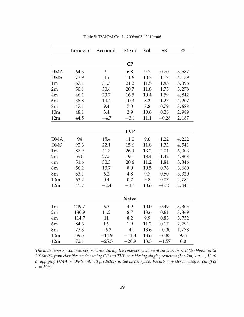
Table 5: TSMOM Crash: 2009m03 - 2010m06

Turnover Accumul. Mean Vol. SR Φ

CP

DMA 64.3 9 6.8 9.7 0.70 3, 582DMS 73.9 16 11.6 10.3 1.12 4, 1591m 67.1 31.5 21.2 11.5 1.85 5, 3962m 50.1 30.6 20.7 11.8 1.75 5, 2784m 46.1 23.7 16.5 10.4 1.59 4, 8426m 38.8 14.4 10.3 8.2 1.27 4, 2078m 47.1 9.4 7.0 8.8 0.79 3, 68810m 48.1 3.4 2.9 10.6 0.28 2, 98912m 44.5 −4.7 −3.1 11.1 −0.28 2, 187

TVP

DMA 94 15.4 11.0 9.0 1.22 4, 222DMS 92.3 22.1 15.6 11.8 1.32 4, 5411m 87.9 41.3 26.9 13.2 2.04 6, 0032m 60 27.5 19.1 13.4 1.42 4, 8034m 51.6 30.5 20.6 11.2 1.84 5, 3466m 56.2 10.7 8.0 10.5 0.76 3, 6608m 53.1 6.2 4.8 9.7 0.50 3, 32010m 63.2 0.4 0.7 9.8 0.07 2, 78112m 45.7 −2.4 −1.4 10.6 −0.13 2, 441

Naive

1m 249.7 6.3 4.9 10.0 0.49 3, 3052m 180.9 11.2 8.7 13.6 0.64 3, 3694m 114.7 11 8.2 9.9 0.83 3, 7526m 84.6 1.9 1.9 11.2 0.17 2, 7918m 73.3 −6.3 −4.1 13.6 −0.30 1, 77810m 59.5 −14.9 −11.3 13.6 −0.83 97612m 72.1 −25.3 −20.9 13.3 −1.57 0.0

The table reports economic performance during the time-series momentum crash period (2009m03 until2010m06) from classifier models using CP and TVP, considering single predictors (1m, 2m, 4m, ..., 12m)or applying DMA or DMS with all predictors in the model space. Results consider a classifier cutoff ofc = 50%.

29

the naive approach. However, as mentioned before, sticking solely to a very fast look-backperiod can induce lower performances in the long-run, then recognizing the time-varyingimportance of different momentum speeds is crucial for a stronger portfolio with lowerrisk and drawdowns. Since the DMA and DMS settings were built exactly with the goalof learning different momentum speed dynamics, we can notice that they provide strongportfolio performances not just on the long-run as we have shown in last sections, but alsoduring the 2009 momentum crash period. Table (5) also makes clear the advantage of al-lowing time-varying parameters, since during bad periods the economic relations amongfinancial data can change in a matter of few periods. When the investor considers theDMS-TVP approach, she is able to obtain 22.1% of accumulated returns during the mo-mentum crash with a robust SR of 1.32! It means that a mean-variance investor would pay4,541 bps to switch from the 12-month naive approach to the DMS-TVP method.

In order to provide evidences that the dynamic classifier method with TVP is capableof learning from past mistakes and assign higher probabilities for those look-back periodsthat are performing better in the recent past and reducing probabilities for trends thatno longer exists, Figure (2) shows inclusion probabilities for momentum predictors of 1,2, 10 and 12-months, averaged across all different assets. For a given asset, a inclusionprobabilitity (IP) for a specific momentum speed L can be defined as

IPL =M

∑j=1

1(j⊂J)p(

Mj|Dt)

where J represents the subset of models containing the specific momentum predictor Land 1(j⊂J) is an indicator function taking the value of 1 if the model j is cointained on J.Hence, a higher IPL means that models with the momentum predictor L are performingbetter in the recent past and then receiving higher model probabilities. Since we averageIPL for all assets available at the time period, Figure (2) can give us a sense of the over-all importance of longer ou shorter trends over time and in special the 2009 momentumCrash.

It is evident that as soon as the rebound starts at the beginning of 2009, models withlook-back period of 10 and 12-month momentum predictors sequentially received lowerprobabilities while the 1-month momentum predictor increase in importance. The 2-month momentum predictor continued to oscillate around its older inclusion probabili-ties, but remaining higher than longer momentum predictors. It is interesting to noticethat since the 2009 Crash, longer momentum speeds remained much less important thanfaster momentum speeds, in line with recent evidences on the increase of trend breaks

30

Figure 2: Mean inclusion probabilities - Momentum speeds

since 2010 (Baltas and Kosowski, 2020, Garg et al., 2020 and Garg et al., 2021 ). At the sametime, the 1-month look-back period remains as the predictor with highest inclusion prob-abilities. In fact, although longer trends were more important than they are nowadays,the 1-month momentum already had greater importance even before the Great Recession.Therefore, Figure (2) gives evidences that sequentially learning the importance of eachmomentum speed, combining or selecting those different informations to generate out-of-sample signal forecasts was able to deal with the 2009 trend break problem with greatsucess, as Table (5) highlights.

31

Table 6: Economic Performance: 2010m07 - 2020m09

Turnover Mean Vol. Max.DD SR Φ

CP

DMA 65 9.7 10.0 14.8 0.97 470.6DMS 80.4 11.8 10.0 10.4 1.18 698.91m 64.7 11.8 10.0 10.1 1.18 692.92m 47.9 9.8 10.0 11.2 0.98 484.54m 47.4 7.0 10.0 18.9 0.70 197.26m 41.7 8.1 10.0 14.9 0.81 311.18m 38.3 9.0 10.0 12.5 0.90 407.510m 35.7 9.0 10.0 16.8 0.90 406.312m 35.2 8.7 10.0 15.5 0.87 372.7

TVP

DMA 93.4 9.4 10.0 12.8 0.94 440.1DMS 114.5 11.0 10.0 13.7 1.10 609.31m 82.7 9.3 10.0 11.1 0.93 433.52m 60.5 7.2 10.0 14 0.72 222.64m 54.2 7.4 10.0 17 0.74 233.56m 48.1 8.4 10.0 13.5 0.84 338.28m 45.5 7.5 10.0 17.2 0.75 246.810m 39.0 6.3 10.0 21.2 0.63 128.312m 48.4 6.1 10.0 21.7 0.61 108.2

Naive

1m 356.8 0.8 10.0 27 0.08 −412.72m 225.3 5.4 10.0 13 0.54 31.64m 163.8 2.9 10.0 19.5 0.29 −216.06m 127.7 2.8 10.0 17.4 0.28 −219.28m 118.5 2.4 10.0 13.5 0.24 −265.810m 95.1 5.4 10.0 16.3 0.54 38.812m 89.1 5.0 10.0 15.5 0.50 0.0

The table reports economic performance after the time-series momentum crash period (2010m07 until2020m09) from classifier models using CP and TVP, considering single predictors (1m, 2m, 4m, ...,12m) or applying DMA or DMS with all predictors in the model space. Results consider a classifiercutoff of c = 50%. All strategies are scaled to an ex-post annualized volatility of 10%.

32

5.1 The post-Crash period

After the Great Recession, the number of turning points increased considerably for differ-ent assets. Garg et al. (2020) show that there is a negative relation among the number ofturning points and Sharpe Ratios of TSMOM strategies. In order to show the robustnessof our dynamic classifier approach on the subsequent periods of the 2009 Crash, Table (6)displays portfolio results from July 2010 to September 2020.

Our results confirm the weakness of the Naive-TSMOM strategies on the post GreatFinancial Crisis, as observed in the works of Rubesam (2020), Garg et al. (2020) and Bal-tas and Kosowski (2020). The naive benchmark strategy obtained a Sharpe ratio of 0.50during the period, which means a reduction of about 40% compared to the whole sampleevaluated before and the results remain weaker regardless of the look-back period consid-ered.

When our binary classifier is applied, the optics is still very optimistic. Indeed, whatcan be seen is a much stronger performance for the subsequent period of the 2009 Crashcompared to the Naive-TSMOM. For any single predictor setting, the performances arebetter than the naive benchmark. Portfolio improvements are observed regardless of thedynamics induced in coefficients. The DMS-TVP was able to generate a Sharpe Ratio of1.10, a 120% increase in relation to the naive benchmark, which would require an annual-ized management fee of 609.3 bps for the investor give up the traditional naive benchmarkto start using the DMS-TVP model. It is interesting to notice that, for this particular sam-ple period, the CP setting performed even better than the model settings where TVP areallowed. The DMS-CP have showed a Sharpe ratio of 1.18, representing 698.9 bps as man-agement fees to use switch from the naive benchmark to this particular model setting.These results demonstrate evidence of no incremental performance for dynamics on co-efficients and a simple constant parameter binary classifier model is able to successfullydeal with the amount of turning points in the post 2009 Crash. The most important pat-tern observed in the period is the strong performance of the single 1-month momentumpredictor. The results are in line with Figure (2), where the 1-month look-back emergedwith higher inclusion probabilities than longer/slower momentum measures.

Finally, just for the sake of curiosity, one of the highest drawdowns from the naivebenchmark strategy was exactly during the Covid period. Since April 2020 to Septemberof that year, the traditional 12-month time-series momentum strategy accumulated 8.6%of return losses. The performance was not worse in 2020 because many assets at the verybeginning of the year were signaling negative momentum such that, when the market

33

really suffered huge losses in March, the strategy was able to profit from negative trends,earning 8.7% in that month. Hence, from March to Semptember, the naive benchmarkaccumulated just 0.6% of losses. At the other hand, the DMS-TVP was able to deliver18.4% of accumulated returns from March to September. Its CP counterpart, the DMS-CPmodel, also performed quite well in this period, earning 15.0% of accumulated returns.

Therefore, Table (6) gives evidences that the the dynamic classifier performance is ro-bust even for periods of higher trend breaks. Since dynamic model probabilities are ableto dynamically assign higher or lower probabilities to models with different momentumspeeds, as we have showed in Section 3, new financial environments are not enough toweaken its final portfolio performance. What we actually see is the oposite, where periodof higher changes in financial trends are accompanied by better returns adjusted for risk.

6 Conclusion

Since the work of Moskowitz et al. (2012), the literature on trend-following strategies hasgrown rapidly and its applicability has spread throughout the financial industry. How-ever, there is still a lack of discussion of how to incorporate econometric models to help in-vestors to learn about better momentum speeds over time. From the investor perspective,the better understanding of the time-varying relations from past accumulated returns andfuture return signals are crucial for portfolio construction. Recent evidences has shownthat standard discretionary time series strategies tend to suffer stronger breaking trendsand crashes, which dramatically harm portfolio returns adjusted for risk.

In this study we propose the use of a dynamic binary classifier model where investorscan sequentially learn the sensitivities between past returns and future signals. Imposingtime-varying parameters, the model is able to adapt to changes in the financial market,moving faster from momentum to reversal if it is empirically wanted. Also, by the use ofdynamic model probabilities, the approach is able to recognize sudden turning points, se-quentially switching from slow to fast momentums after a market rebound, dramaticallyreducing drawdowns and momentum crashes. Our results show not just better forecast-ing accuracy gains compared to the naive time series momentum strategy but also thatan investor using the dynamic classifier approach earns annualized Sharpe Ratios muchhigher than the naive benchmark. We analyze different model specifications, cutoffs andsubsamples and results still have shown robustness. The performances remained quitestrong even after the Great Financial Crisis. Considering a mean-variance investor with aquadratic utility, we show that she will be willing to pay an annualized management fee

34

of 425.1 basis points to switch from the naive 12 months time series momentum strategyto our dynamic classifier approach with model selection and time-varying coefficients.Therefore, it generates not just strong portfolio performance, but great economic utilitygains for investors. We show that utility gains are even higher during the 2009 momen-tum Crash and in the last decade. Those are good news for portfolio managers who areinterested in improving trend investment strategies in a unstable financial world with highmodel uncertainties and rapid and complex changes over time.

The strong results obtained using future contracts, in special among commodity fu-tures, motivate us to consider as an extension for future research the use of a larger setof commodities to be analyzed. Also, we also pretend to extend to a larger cross-sectionof equity returns. Inspired by the recent works of Jiang, Kelly, and Xiu (2020) and Kelly,Moskowitz, and Pruitt (2021), where the authors also apply econometric forecasting mod-els to portfolio construction, our future interest is to test the dynamic classifier approachfor cross-sectional momentum strategies, building long-short portfolios by different quan-tiles of model ranking predictions. We believe that this extension can be seen as a strongreturn forecasting model competitor for the recent advances in the momentum literature.

35

Appendix: Aditional Results

Bayesian portfolio decision

We explain here the implicit cutoff selection obtained from an Bayesian decision perspec-tive. The main goal of the Bayesian investor is to sequentially select the action that maxi-mizes expected utility. For each period of time t and for each asset available i, the investoris faced with two simple actions within the set of possible actions A = {Long, Short}, i.e.,she can open a long or short position for asset i. After the realization of the true returnvalue, each given action can produce a different utility for the investor and this utility willdepend on the actual return direction for that period t. If the investor went long an assetand after observing its true direction it was actually up (positive), then the investor shouldreceive a positive utility gain. The same would apply if she went short an asset that wasactually down (negative). When the action made by the investor does not match the ac-tual direction, she should lose utility. The Table below summarizes the possible actionsand their final outcomes.

Actual DirectionsPositive Negative

Actions (A) Long UL,P UL,N

Short US,P US,N

where

• UL,P is the utility when a Long position is opened and the actual return was Positive;

• UL,N is the utility when a Long position is opened and the actual return was Nega-tive;

• US,P is the utility when a Short position is opened and the actual return was Positive;

• US,N is the utility when a Short position is opened and the actual return was Negative

Since we consider a quadratic utility for the mean-variance investor in the same spiritof Equation (22), we compute:

• UL,P = R(+) −γ

2(1+γ)σ(+)

36

• UL,N = R(−) −γ

2(1+γ)σ(−)

• US,P = −R(+) −γ

2(1+γ)σ(+)

• US,N = −R(−) −γ

2(1+γ)σ(−)

where the bar upscript represents historical sample estimates until the decision period andthe signs subscripts in parentheses filter for positive or negative historical observations.Hence, the investor considers those utility estimates as possible final outcomes before as-suming a specific action.

At the end of time t− 1, the investor will choose the action that maximizes his expectedutility for time t, where the expected utility for each action will depend on the forecastingoutput for asset i from the model she is considering. As an example, suppose the investoris willing to open a position on a specific asset i and will consider to use DMA as a fore-casting model to decide the probability of a positive return on the next period. Hence, shewill use the forecasting output as in Equation (17) to compute expected utility for a Longposition (E[U(Long)]) and for Short position (E[U(Short)]):

E[U(Long)] = sDMAt|t−1 UL,P + (1− sDMA

t|t−1 )UL,N

and

E[U(Short)] = sDMAt|t−1 US,P + (1− sDMA

t|t−1 )US,N

If E[U(Long)] ≥ E[U(Short)], the investor opens a long position on asset i, and goesshort otherwise.

Table (7) below show results when the investor sequentially applies the mechanismexplained above for each asset available across time. It is important to highlight herethat the Bayesian decision is applied just to produce trading position signs, but portfolioconstruction and weighing still follows the same structure as Equations (18) and (19).

The general conclusions in Table (7) follow the same we have obtained before in themain body of the paper.

37

Table 7: Economic - Expected Utility decision

Turnover Mean Vol. Max.DD SR Φ

CP

DMA 68.2 10.3 10.0 14.5 1.030 214.480DMS 79.7 11.2 10.0 14.5 1.120 306.9101m 75.4 7.3 10.0 25.3 0.730 −87.4702m 59.5 6.2 10.0 23 0.620 −186.9104m 52.9 8 10.0 20.4 0.8 −11.2606m 45.7 8.1 10.0 14.1 0.810 −7.2608m 45.6 8.8 10.0 18.4 0.880 69.84010m 43.9 8.8 10.0 17.1 0.880 62.78012m 42.6 6.3 10.0 17.5 0.630 −183.630

TVP

DMA 78 10.5 10.0 11.8 1.050 238.070DMS 92.4 11.1 10.0 12.5 1.110 302.4501m 80.1 8.9 10.0 16.5 0.890 82.0402m 63 6.3 10.0 25.8 0.630 −177.3404m 55.4 6.9 10.0 26.1 0.690 −118.7306m 49.6 7.6 10.0 16.7 0.760 −49.1808m 47 9.2 10.0 12.9 0.920 106.04010m 47.1 8.2 10.0 16.7 0.820 7.38012m 47.8 6.4 10.0 15.4 0.640 −175.440

The table reports economic performance from classifier models using constant parameters (CP) and time-varying parameters (TVP), considering single predictors (1m, 2m, 4m, ..., 12m) or applying DMA orDMS with all predictors in the model space. Classifier cutoffs are implicit obtained from a sequentialBayesian decision problem, where the investor selects the best trading action based on its expected utility.All strategies are scaled to an ex-post annualized volatility of 10%.

38

Descriptive Statistics

Table 8: Summary Statistics of Futures Contracts

Futures Start.Date Mean Vol SR

EquitiesS&P500 1982-05 8.7 15.4 0.36Nasdaq 100 1999-09 7.4 24.7 0.23S&P Canada 60 1999-10 4.5 20.5 0.15FTSE 100 1984-06 4.6 18.1 0.1DAX 1990-12 7 22.2 0.25CAC 40 1999-02 0.7 21 -0.02IBEX 35 1992-05 2.1 23.8 0.03FTSE MIB 2004-04 -2.3 25.3 -0.08AEX 1988-11 5.1 20.3 0.14SMI 1990-12 7.8 16.2 0.36Nikkei 225 1990-10 0.3 21.2 -0.1ASX SPI 200 2000-06 4.2 22.3 0.17

BondsUS Tsy Note 2-year 1990-07 1.3 1.5 -0.74US Tsy Note 5-year 1988-06 2.7 3.9 -0.02US Tsy Bond 10-year 1982-06 4.4 6.6 0.14US Tsy Bond 30-year 1980-01 4.6 11.1 0.05Euro Schatz 2-year 1998-11 0.7 9.6 -0.07Euro Bobl 5-year 1999-02 2.4 9.7 0.11Euro Bund 10-year 1998-11 3.8 10.2 0.24Euro Buxl 30-year 2005-10 6.1 12.4 0.4UK Long Gilt 1982-12 2.4 12.2 -0.07Canadian 10-year 1989-10 3.3 9.1 0.09Japanese 10-year 1987-01 3.9 12.4 0.08

CurrenciesAUD/USD 1983-04 0.8 36.6 -0.08CAD/USD 2007-08 -4.8 40.1 -0.12CHF/USD 2006-02 -3.2 33.1 -0.12EUR/USD 1990-05 0.5 51.3 -0.08GBP/USD 2005-11 -2 47.1 -0.07JPY/USD 2007-01 0.4 27 0.02NZD/USD 1980-01 3.1 17.4 -0.05SEK/USD 1980-01 6.4 34.5 0.08

39

Table 9: Summary Statistics of Futures Contracts (Continued)

Futures Start Date Mean Vol. SR

CommoditiesLight crude oil 1980-01 0.6 25.1 -0.12Brent crude oil 1980-01 -0.9 32.7 -0.15Heating oil 1980-01 1.3 15.3 -0.18Natural gas 1980-02 1.2 17.8 -0.15RBOB gasoline 1980-01 1.4 36.3 -0.04Copper 1980-01 0.7 27.3 -0.12Gold 2006-04 3.4 36.5 0.11Palladium 2006-04 2.6 24.1 0.07Platinum 2006-04 4.6 31.7 0.15Silver 1980-01 1.1 24.6 -0.09Feeder cattle 2006-04 3.5 33.3 0.11Live cattle 1980-01 -0.4 30 -0.14Lean hogs 1980-01 -1.2 35.3 -0.19Corn 1980-01 -0.3 30.5 -0.15Oats 1980-01 2.6 35.4 -0.02Soybean oil 1980-01 0.4 31.8 -0.16Soybean meal 1980-01 -0.5 41.3 -0.08Soybeans 1987-02 2.7 11.4 0.01Wheat 1980-01 -0.3 8.8 -0.49Cocoa 1980-01 -0.7 11.9 -0.38Coffee 1999-04 -0.3 9.7 -0.16Cotton #2 1980-01 -0.5 10.2 -0.42Lumber 1980-01 -1.1 11.6 -0.44Orange juice 1997-06 2.2 12.8 0.04Sugar #11 2004-05 -1.7 11.2 -0.23

40

References

ASNESS, C. S., T. J. MOSKOWITZ, AND L. H. PEDERSEN (2013): “Value and momentumeverywhere,” The Journal of Finance, 68, 929–985. 3

BALTAS, N. (2015): “Trend-following, risk-parity and the influence of correlations,” inRisk-Based and Factor Investing, Elsevier, 65–95. 3

BALTAS, N. AND R. KOSOWSKI (2013): “Momentum strategies in futures markets andtrend-following funds,” in Paris December 2012 Finance Meeting EUROFIDAI-AFFI Paper.3

——— (2020): “Demystifying time-series momentum strategies: volatility estimators,trading rules and pairwise correlations,” Market Momentum: Theory and Practice", Wi-ley. 3, 15, 21, 27, 31, 33

BARROSO, P. AND P. SANTA-CLARA (2015): “Momentum has its moments,” Journal ofFinancial Economics, 116, 111–120. 6

BECKMANN, J., G. KOOP, D. KOROBILIS, AND R. A. SCHÜSSLER (2020): “Exchange ratepredictability and dynamic Bayesian learning,” Journal of Applied Econometrics, 35, 410–421. 12

CAMPBELL, J. Y. AND S. B. THOMPSON (2008): “Predicting excess stock returns out ofsample: Can anything beat the historical average?” The Review of Financial Studies, 21,1509–1531. 4

CATANIA, L., S. GRASSI, AND F. RAVAZZOLO (2019): “Forecasting cryptocurrencies undermodel and parameter instability,” International Journal of Forecasting, 35, 485–501. 5

CHINCO, A., A. D. CLARK-JOSEPH, AND M. YE (2019): “Sparse signals in the cross-section of returns,” The Journal of Finance, 74, 449–492. 4, 19

DANGL, T. AND M. HALLING (2012): “Predictive regressions with time-varying coeffi-cients,” Journal of Financial Economics, 106, 157–181. 4, 5

DANIEL, K. AND T. J. MOSKOWITZ (2016): “Momentum crashes,” Journal of Financial Eco-nomics, 122, 221–247. 6, 27

FLEMING, J., C. KIRBY, AND B. OSTDIEK (2001): “The economic value of volatility timing,”The Journal of Finance, 56, 329–352. 7, 20

41

GAO, L., Y. HAN, S. Z. LI, AND G. ZHOU (2018): “Market intraday momentum,” Journalof Financial Economics, 129, 394–414. 3

GARG, A., C. L. GOULDING, C. R. HARVEY, AND M. MAZZOLENI (2020): “Breaking BadTrends,” Available at SSRN. 6, 27, 31, 33

——— (2021): “Momentum turning points,” Available at SSRN 3489539. 6, 27, 31

GEORGOPOULOU, A. AND J. WANG (2017): “The trend is your friend: Time-series momen-tum strategies across equity and commodity markets,” Review of Finance, 21, 1557–1592.3

GU, S., B. KELLY, AND D. XIU (2020): “Empirical asset pricing via machine learning,” TheReview of Financial Studies, 33, 2223–2273. 5, 19

GUPTA, T. AND B. KELLY (2019): “Factor momentum everywhere,” The Journal of PortfolioManagement, 45, 13–36. 4

HAN, Y., G. ZHOU, AND Y. ZHU (2016): “A trend factor: Any economic gains from usinginformation over investment horizons?” Journal of Financial Economics, 122, 352–375. 6

HURST, B., Y. H. OOI, AND L. H. PEDERSEN (2013): “Demystifying managed futures,”Journal of Investment Management, 11, 42–58. 3

——— (2017): “A century of evidence on trend-following investing,” The Journal of PortfolioManagement, 44, 15–29. 3

HUTCHINSON, M. C. AND J. O’BRIEN (2020): “Time series momentum and macroeco-nomic risk,” International Review of Financial Analysis, 69, 101469. 3

HWANG, Y. (2019): “Forecasting recessions with time-varying models,” Journal of Macroe-conomics, 62, 103153. 5

JEGADEESH, N. AND S. TITMAN (1993): “Returns to buying winners and selling losers:Implications for stock market efficiency,” The Journal of Finance, 48, 65–91. 3

JIANG, J., B. T. KELLY, AND D. XIU (2020): “(Re-) Imag (in) ing Price Trends,” ChicagoBooth Research Paper. 6, 17, 19, 35

JOHANNES, M., A. KORTEWEG, AND N. POLSON (2014): “Sequential learning, predictabil-ity, and optimal portfolio returns,” The Journal of Finance, 69, 611–644. 4

42

KELLY, B. T., T. J. MOSKOWITZ, AND S. PRUITT (2021): “Understanding momentum andreversal,” Journal of Financial Economics, 140, 726–743. 35

KIM, A. Y., Y. TSE, AND J. K. WALD (2016): “Time series momentum and volatility scal-ing,” Journal of Financial Markets, 30, 103–124. 8, 15

KOOP, G. AND D. KOROBILIS (2012): “Forecasting inflation using dynamic model averag-ing,” International Economic Review, 53, 867–886. 5

——— (2013): “Large time-varying parameter VARs,” Journal of Econometrics, 177, 185–198.5, 12

LAVINE, I., M. LINDON, M. WEST, ET AL. (2020): “Adaptive variable selection for sequen-tial prediction in multivariate dynamic models,” Bayesian Analysis. 12

LEVY, B. P. AND H. F. LOPES (2021a): “Dynamic Ordering Learning in Multivariate Fore-casting,” arXiv preprint arXiv:2101.04164. 5

——— (2021b): “Dynamic Portfolio Allocation in High Dimensions using Sparse Risk Fac-tors,” arXiv preprint arXiv:2105.06584. 4

LIM, B. Y., J. G. WANG, AND Y. YAO (2018): “Time-series momentum in nearly 100 yearsof stock returns,” Journal of Banking & Finance, 97, 283–296. 3

LIU, L., Z. PAN, AND Y. WANG (2021): “What can we learn from the return predictabilityover the business cycle?” Journal of Forecasting, 40, 108–131. 5

MARQUERING, W. AND M. VERBEEK (2004): “The economic value of predicting stockindex returns and volatility,” Journal of Financial and Quantitative Analysis, 39, 407–429.20

MCCORMICK, T. H., A. E. RAFTERY, D. MADIGAN, AND R. S. BURD (2012): “Dynamiclogistic regression and dynamic model averaging for binary classification,” Biometrics,68, 23–30. 5, 9, 11, 12

MOSKOWITZ, T. J., Y. H. OOI, AND L. H. PEDERSEN (2012): “Time series momentum,”Journal of financial economics, 104, 228–250. 1, 3, 7, 8, 19, 34

PRADO, R. AND M. WEST (2010): Time series: modeling, computation, and inference, CRCPress. 10

43

RAFTERY, A. E., M. KÁRNY, AND P. ETTLER (2010): “Online prediction under modeluncertainty via dynamic model averaging: Application to a cold rolling mill,” Techno-metrics, 52, 52–66. 10, 12

RAPACH, D. E., J. K. STRAUSS, AND G. ZHOU (2010): “Out-of-sample equity premiumprediction: Combination forecasts and links to the real economy,” The Review of FinancialStudies, 23, 821–862. 4

RUBESAM, A. (2020): “The Long and the Short of Risk Parity,” Available at SSRN 3468071.3, 15, 19, 21, 33

WELCH, I. AND A. GOYAL (2008): “A comprehensive look at the empirical performanceof equity premium prediction,” The Review of Financial Studies, 21, 1455–1508. 4, 5

WEST, M. AND J. HARRISON (1997): Bayesian forecasting and dynamic models, Springer Sci-ence & Business Media. 10

ZHAO, Z. Y., M. XIE, AND M. WEST (2016): “Dynamic dependence networks: Financialtime series forecasting and portfolio decisions,” Applied Stochastic Models in Business andIndustry, 32, 311–332. 12

44