transport phenomena through porous screens and openings
TRANSCRIPT
Transport phenomena through porous screens and
openings: from theory to greenhouse practice
A. A. F. Miguel
Proefschrift
ter verkrijging van de graad van
doctor
op gezag van de rector magnificus,
Dr. C. M. Karssen,
in het openbaar te verdedigen
op woensdag 25 februari 1998
des namiddags te vier uur in de aula
van de Landbouwuniversiteit te Wageningen
l bM c\ <-L f9&}
CIP-DATA KONINKLIJKE BIBLIOTHEEK, DEN HAAG
Miguel, A. A. F.
Transport phenomena through porous screens and openings: from theory to
greenhouse practice I A.A.F. Miguel. [S.l.:s.n]
Thesis Wageningen. - With Ref. - With Summaries in English, Dutch,
Portugese and Chinese
ISBN 90-5485-847-8
Subject headings: mass and heat exchange / porous materials / openings /
screened greenhouses.
Cover: Fluid flow around a solid body
This thesis is also available as publication nr. 98-2 , ISBN 90-5485-843-5
of the DLO Institute of Agricultural and Environmental Engineering
(IMAG-DLO), P.O.Box 43, NL-6700 AA Wageningen, The Netherlands
ABSTRACT
Miguel, A. A. F. 1998. Transport phenomena through porous screens and openings: from theory to greenhouse practice. Ph.D. Dissertation, Landbouwuniversiteit, Wageningen. Also available as a publication of Instituut voor Milieu en Agritechniek (IMAG-DLO) Wageningen, Netherlands. 129 pp.; 44 figs.; 9 tables; 112 refs.; English, Dutch, Portuguese and Chinese summaries.
Keywords: free and forced convective mass exchange, fluctuating flow, free
convective heat transfer, porous screens, window openings, screened
greenhouses.
The study of transport phenomena in multi-zone enclosures with permeable
boundaries is fundamental for indoor climate control management. In this
study, aspects concerning the air exchange through porous screens and
openings, and heat transfer between the enclosure surface and inside air, were
analysed. Basic physical laws were the starting point during the construction of
the models. To illustrate the practical side of the research performed, the
formulation developed was applied to the study of convective heat exchange
within screened greenhouses, as well as to the study of airflow through
greenhouse screens and window apertures.
Concerning the airflow through porous screens and window openings, the
results obtained thoroughly demonstrate the importance of inertia and viscous
effects, as well as window openings' geometry effects, on fluid flow. The
airflow characteristics of porous screens and the structure of fluctuation of
wind velocity, were quantified.
Regarding the study of free convection heat transfer within a screened
greenhouse, the convective heat transfer coefficients between the air and the
downward and the upward surfaces of the screen were obtained, among other
Abstract
results.
The results obtained from this study can greatly contribute, in general, to a
better climate control management of multi-zone enclosures, and specifically,
to an improved application of porous screens and window apertures.
CONTENTS
ABSTRACT
PREFACE
1. INTRODUCTION
1.1 Preliminary remarks 1
1.2 Transport phenomena in screened greenhouses - the importance
of study of porous screens 2
1.2.1 Reasons for studying screened greenhouses 2
1.2.2 Modelling the influence of porous screens in
greenhouses: interest, previous research and needs 2
1.3 Aim 4
1.4 Overview of the thesis 4
1.5 References 6
2. FORCED FLUID MOTION THROUGH OPENINGS AND PORES
2.1 Introduction 9
2.2 Mathematical formulation 10
2.2.1 The equation of motion using the method of
volume averaging 11
2.2.2 The range of validity of the motion equation 13
2.2.3 Motion equation for a permeable medium 15
2.2.4 Simplified motion equation for pores and openings 15
2.3 Experimental study 17
Contents
2.3.1 Description of experiments 18
2.3.2 Results and discussion 19
2.4 Conclusions 23
2.5 References 23
2.6 Appendix 25
2.7 Nomenclature 26
3. ANALYSIS OF AIR EXCHANGE INDUCED BY FLUCTUATING
EXTERNAL PRESSURES IN ENCLOSURES
3.1 Introduction 29
3.2 Mathematical formulation 30
3.2.1 General description of the model 30
3.2.2 Fluctuating pressure inside an enclosure where air
is exchanged with the outside through one opening
with large free area or through a structure with narrow
open ings or pores 32
3.3 Air exchange in a multi-zone enclosure 38
3.3.1 Network equations 38
3.3.2 Experimental study 39
3.4 Conclusions 45
3.5 References 46
3.6 Nomenclature 48
4. MODELLING MIXED FLUID MOTION THROUGH POROUS MEDIA:
DESCRIPTION OF MATRIX-FLUID INTERACTION
4.1 Introduction 49
Stellingen/Propositions
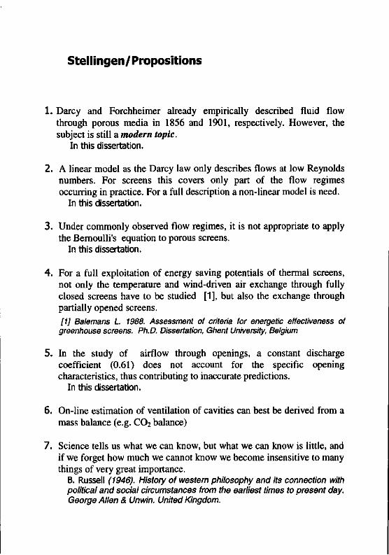
1. Darcy and Forchheimer already empirically described fluid flow through porous media in 1856 and 1901, respectively. However, the subject is still a modern topic.
In this dissertation.
2. A linear model as the Darcy law only describes flows at low Reynolds numbers. For screens this covers only part of the flow regimes occurring in practice. For a full description a non-linear model is need.
In this dissertation.
3. Under commonly observed flow regimes, it is not appropriate to apply the Bernoulli's equation to porous screens.
In this dissertation.
4. For a full exploitation of energy saving potentials of thermal screens, not only the temperature and wind-driven air exchange through fully closed screens have to be studied [1], but also the exchange through partially opened screens. [1] Balemans L. 1988. Assessment of criteria for energetic effectiveness of greenhouse screens. Ph.D. Dissertation, Ghent University, Belgium
5. In the study of airflow through openings, a constant discharge coefficient (0.61) does not account for the specific opening characteristics, thus contributing to inaccurate predictions.
In this dissertation.
6. On-line estimation of ventilation of cavities can best be derived from a mass balance (e.g. C02 balance)
7. Science tells us what we can know, but what we can know is little, and if we forget how much we cannot know we become insensitive to many things of very great importance.
B. Russell (1946). History of western philosophy and its connection with political and social circumstances from the earliest times to present day. George Allen & Unwin. United Kingdom.
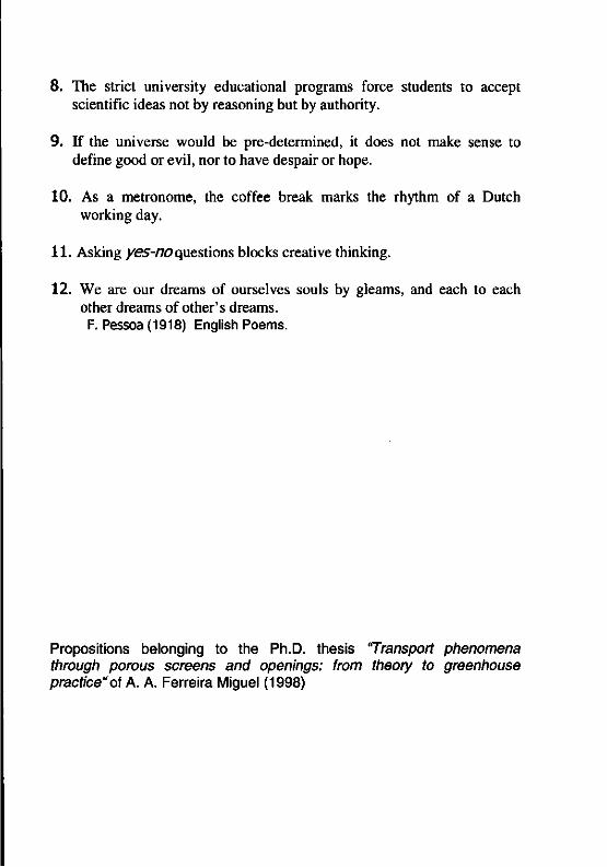
8. The strict university educational programs force students to accept scientific ideas not by reasoning but by authority.
9. If the universe would be pre-determined, it does not make sense to define good or evil, nor to have despair or hope.
10. As a metronome, the coffee break marks the rhythm of a Dutch working day.
11. Asking yes-no questions blocks creative thinking.
12. We are our dreams of ourselves souls by gleams, and each to each other dreams of other's dreams. F. Pessoa (1918) English Poems.
Propositions belonging to the Ph.D. thesis 'Transport phenomena through porous screens and openings: from theory to greenhouse practice"of A. A. Ferreira Miguel (1998)
Contents
4.2 Fluid flow through a permeable medium: basic equations 50
4.3 Fluid absorption within a porous medium and the effect on
fluid flow 52
4.3.1 Mass change in the subsystem matrix-fluid 53
4.3.2 Effects on fluid flow 54
4.4 Methodologies for measuring parameters Çv, C^, K, a, s and Xeff 55
4.5 Experimental determination of parameters Çv and
Çs, for different porous media 56
4.6 Final comments 59
4.7 References 60
4.8 Appendix 61
4.9 Nomenclature 62
5. ANALYSIS OF THE AIRFLOW CHARACTERISTICS OF GREENHOUSE
SCREENING MATERIALS
5.1 Introduction 65
5.2 Pressure drop and flow relationship 66
5.3 Motion equation and airflow characteristics of porous screens 66
5.4 Experimental study 68
5.5 Results and discussion 72
5.6 Conclusions 77
5.7 References 77
5.8 Appendix 78
5.9 Nomenclature 80
Contents
6. PHYSICAL MODELLING OF A NATURAL VENTILATION THROUGH
SCREENS AND WINDOWS IN GREENHOUSE
6.1 Introduction 83
6.2 Theory 85
6.2.1 Motion equation 85
6.2.2 Driving potential 86
6.3 Experimental study 89
6.4 Results and discussion 92
6.4.1 Wind velocity and wind pressure 92
6.4.2 Airflow through porous screens and openings 94
6.5 Conclusions 99
6.6 References 100
6.7 Appendix 102
6.8 Nomenclature 104
7. FREE CONVECTION HEAT TRANSFER IN SCREENED GREENHOUSE
7.1 Introduction 107
7.2 Theoretical background 108
7.2.1 Heat transfer by convection 109
7.2.2 Flow characteristics criterion 110
7.3 Experimental arrangement 111
7.4 Description of experiments 113
7.5 Results 114
7.6 Discussion 119
7.7 Conclusions 121
7.8 References 122
7.9 Nomenclature 123
Contents
8. FINAL DISCUSSION AND CONCLUSION
8.1 Air infiltration in enclosure with pores and openings 125
8.2 Free convective heat transfer inside a screened greenhouse 127
8.3 Final remarks 128
8.4 References 129
SAMENVATTING
SUMÄRIO
SUMMARY
$1 £
LIST OF AUTHOR REFEREED PUBLICATIONS

PREFACE
This thesis results from my Ph.D. study at IMAG-DLO and at Wageningen
Agricultural University (WAU), under a contract financed by Fundaçào C.
Gulbenkian and JNICT (Portugal), and by Novem bv and Landbouwschap (the
Netherlands). It finishes a very pleasant staying in the Netherlands, which I
hope will stand for a close cooperation between these institutions and my
University (Department of Physics of Evora University) in Portugal.
This thesis owes its existence to many people (within and outside the
university community), whose guidance, encouragement and friendship were
essential for the reaching of my goals. I would like to thank all of them.
First, I would like to express my gratitude and appreciation to Prof. Dr. Ir. G.
P. A. Bot and to Prof. Dr. Ana Maria Silva, my promoters, for the guidance and
advice they gave me during this study.
I am deeply indebted to Ir. N. J. van de Braak, for his assistance, inspiration
and constructive criticism during all of the Ph.D. study.
My sincere gratitude to Dr. Ir. H. F. de Zwart for his assistance on making
some computational programmes, mainly the programmes used to control the
experimental set-up.
I thank Mr. H. Loeffen for his valuable help in some experimental
measurements. I gratefully acknowledge the help of Ir. A. van't Ooster, Ir. J. J.
G. Breuer and Mr. A. Ruisch for the setting of my experiments.
Grateful acknowledgements are due to my department colleagues in the
Netherlands and in Portugal for many valuable discussions and thoughtful
suggestions, in particular to Dr. Ir. J. C. Bakker (IMAG-DLO), Dr. Ir. W. K. P.
van Loon (WAU), Dipl. Phys. J. A. Stoffers (IMAG-DLO), and to Prof. Dr. A.
Heitor dos Reis (University of Evora).
On a personal note, I would like to express my thanks to all outside the
university community, who contributed with their friendship for a pleasant
Preface
staying in the Netherlands, in particularly to the couple Barros. I am also
indebted to Ir. Ana I. Costa, for her never-failing support and continuous
friendship.
As in all of my life, I have been greatly supported by my mother and my
sister. I dedicate this book to my father and my grand-parents, will live forever
in my heart.
1. INTRODUCTION
1.1 PRELIMINARY REMARKS
The study of transport phenomena is an important topic in science and engineering.
This is due to the essential (and sometimes decisive) role they play in distinct natural
and industrial processes (geothermal operations, indoor climate control in buildings,
flow over the earth's surface, drying and cooling processes, etc.).
In order to solve problems in transport phenomena, it is necessary to approach the
specific problems from a general physical description. This leads to models which
allow us to predict the phenomena described under a variety of conditions, with
adequate accuracy. The physical principles applied in the building of these models are
the conservation of mass, momentum and energy, and the relations between fluxes and
driving forces. This results in non-linear differential equations, in space and time, from
which analytical solutions can be obtained, although only in the simplest cases.
Usually, these equations have to be solved with the help of numerical techniques like
Euler and other integration technique for lumped parameter problem, or like the finite-
difference and finite volume method for distributed parameter problem [1,2].
Unfortunately, numerical techniques are difficult to use and in most cases not very
practical. Therefore, a very large number of the existing studies deals with
mathematical simplifications, which neglect some physical aspects, while others deal
with simple empirical correlations with an unknown range of validity and
applicability [3,4].
This thesis describes a study of some transport phenomena in multi-zone enclosure,
applied in a screened greenhouse: air infiltrations through screened greenhouses and
free convective heat transfer between the various surfaces and the air within the
greenhouse. Its main purpose is to develop a consistent formulation that is both
Introduction
physically meaningful and useful in practice, and which helps to solve everyday
problems, with higher accuracy and lower computational cost.
1.2 TRANSPORT PHENOMENA IN SCREENED GREENHOUSES - THE IMPORTANCE OF
POROUS S C R E E N S
1.2.1 Reasons for studying screened greenhouses
Protected horticulture is an important contribution to economy of several countries
around the world. In the Netherlands, it provides for about 6.6% of total export value
and represents a value of about 10'° US dollar per year [5]. As a consequence, this
topic is the subject of numerous research initiatives. At first thought, it might appear
that the improvement of products quality and the reduction of production prices should
be the main concerns. However, the related environmental aspects cannot be
neglected, since protected horticulture is an important consumer of fossil fuel and
chemical pesticides.
The potential benefits deriving from the use of screens in protected horticulture have
been increasingly recognised in recent years. In the Netherlands about 75 % of total
greenhouse area is equipped with screens. Thermal screens are a simple, cheap and
effective means of reducing night-time heat loss. Shading screens control the solar
radiation inside a greenhouse, while insect screens prevent the entrance of birds and
insects. Therefore, screen strongly contribute to the reduction of greenhouse heating
and refreshing costs, while being an effective alternative to chemical pesticides in the
control of insect borne diseases.
1.2.2 Modelling the influence of porous screens in greenhouses: interest, previous research and needs
The use of screens in greenhouses has a considerable effect on growing conditions
while they provide an extra resistance to mass, momentum and heat transport between
Chapter 1
the interior and the ambient. The application of screens and thereby the exploitation of
its potentials, has been restricted so far by an improper quantification of the effect on
the growing conditions.
The physical modelling of behaviour of porous screens
• contributes to a better comprehension of physical phenomena around screens
and it allow a correct interpretation of experimental data,
• allows diverse screening strategies to be compared (policy advice),
• improves design tools to optimise the application of screens,
• helps to decide about characteristics of a screening material (commodity
forecasting) in order to support the manufacture of new screening materials,
• implemented in simulation programs helps the improvement of the climate
control (the growing conditions) of a screened greenhouse.
Most literature reviews on greenhouse screens concern its influence on the radiative
climate of greenhouses. The influence of screens on the incoming solar and thermal
radiation have already been successfully modelled [6-9] and the optical or radiometric
characteristics of different materials used for screens have been determined by several
authors [6,10,11].
The influence of screens on convective heat exchange inside greenhouses and the
study of fluid transport through screens have received little attention, and are poorly
understood.
As to our knowledge, only one experimental study (unpublished communication
presented by Stoffers [12] in Cambridge), is concern to the convective heat transfer in
greenhouses divided by a horizontal screen. Fluid transport through screens was
described by Balemans [11], Bailey [13], Sase and Christianson [14], and Kosmos et
al. [15]. The first two, considered only the fluid flow under a Reynolds number
smaller than 1 (Darcy flow regime). Sase and Christianson [14] and Kosmos et al. [15]
considered the fluid transport through a screen to be described by Bernoulli's equation,
and defined the airflow characteristics of a screen according to a "discharge
Introduction
coefficient".
In all studies, the horizontal screen between the greenhouse ground and the roof was
always considered closed between the greenhouse walls. The realistic situation of a
screen opened only slightly [5] was never analysed.
1.3 A IM
Despite the existence of a lot of important studies on the transport phenomena in
multi-zone enclosures with permeable walls, the subject is far from being fully
understood. The study presented in this thesis seeks to clarify some aspects of
transport phenomena occurring in multi-zone enclosures with permeable walls: air
infiltration through enclosures containing openings and pores and heat transfer
between the enclosure surfaces and the inside air. The theory developed is applied to
the study of screened greenhouses and compared with experimental results. Thus, the
study can be used as a tool to increase a more sustainable use of screens and window
apertures.
1.4 OVERVIEW OF THE THESIS
This thesis contains eight chapters. Chapters 2 to 6 are devoted to fluid transport
through multi-zone enclosure with porous materials and openings. Chapter 7 concerns
free (natural) convective heat exchange within the enclosure and Chapter 8 presents
the general conclusions.
In Chapter 2, forced convection through pores and openings is discussed. An
approach based on the momentum equation, developed in terms of the method of
volume averaging is presented. The resulting approach is valid for porous material and
non-porous material, and can be used in computational fluid dynamics to predict the
velocity and pressure throughout the flow field. A simplified and accurate form is also
developed, having a small number of parameters and simple mathematical operations.
4
Chapter 1
In Chapter 3, the approach developed in Chapter 2 together with the mass
conservation equation and the state equation of gases is used to study air exchange
induced by fluctuating pressures. The network flow equations for air exchange in a
multi-zone enclosure and equations for the pressure within each zone with
compressible air are presented.
Fluid transport through permeable materials can also occur due to gradients of
temperature and concentration, or as a result of combined effects (gradients of
temperature, concentration and pressure generated by wind or mechanical means). A
description of mixed convection through porous media supported by thermodynamics
and fluid mechanics basic laws, is presented in Chapter 4. As a result the mass
variation of the medium and the interaction between the matrix and the fluid within
the medium can be studied.
Chapter 5 is devoted to measure the airflow characteristics of porous screens. Nine
different thermal, shading and insect screens were tested by means of a
DC-pressurisation method. Their permeability and porous inertia factor were
determined according to Forchheimer equation (porosity measured with a
microscope). Special attention is given to the airflow characteristics variation
(permeability and porosity) due to screen damage by handling.
In Chapter 6 the approaches presented in Chapter 2 to 4 are applied to the study of
air exchange in a screened greenhouse. This study is complemented with a power-
spectrum analysis of wind velocity, in order to clarify and characterise the structure of
pressure fluctuations (turbulence), and to identify the frequencies of the main eddies
present in the wind field. The fluctuations in the wind velocity are related to the mean
velocity, and the wind pressure is interpreted in terms of the mean wind velocity.
Chapter 7 is devoted to free convective heat transfer inside screened greenhouses.
The heat transfer coefficient at various surfaces is expressed as a relation between
dimensionless Nusselt's number and the Rayleigh's number. Subsequently, an
experimental study is performed to determine free convection heat transfer
Introduction
coefficients (between air and heating pipes, air and horizontal screen, and air and inner
roof surface) in a greenhouse with characteristic lengths close to those of real
greenhouses. The screen surfaces presented some roughness, as the screens used in
greenhouses. Other practical aspects, such as the influence of the position of the
heating pipes in relation to the screen, and the presence of a crop, on the convective
heat transfer between the various surfaces and the air, is discussed.
Finally, Chapter 8 presents the most important conclusions of the present study and
includes a recommendation on possible future research.
1.5 REFERENCES
[1] Patankar, S. V. 1980. Numerical heat transfer and fluid flow, Hemisphere, New
York, USA
[2] Baker, A. J. 1985. Finite element computational fluid mechanics, MacGraw-Hill,
New York, USA
[3] Combarnous, M. and Bernard D. 1988. Modelling free convection in porous
media: from academic cases to real configurations. Proceedings of 1988 National Heat
Transfer Conference, Houston, USA
[4] International Energy Agency (IEA) 1992. Energy conservation in buildings and
community systems programme. Annex 20: Airflow patterns within buildings -
Airflow through large openings on buildings. Report edited by J. van der Maas.
[5] Zwart, H. F. de 1996. Analysing energy-saving options in greenhouse cultivation
using a simulation model. Ph.D. Dissertation, Agricultural University of Wageningen,
The Netherlands
[6] Bailey, B. J. 1981. The reduction of thermal radiation in glasshouse by thermal
screens. Journal of Agricultural Engineering Research 26, 215-224
[7] Rosa, R. 1988. Solar and thermal radiation inside a multispan greenhouse, Journal
of Agricultural Engineering Research 40, 285-295
[8] Silva, A. M., Miguel, A. F. and Rosa, R. 1991. Thermal radiation inside a single
Chapter 1
span greenhouse with a thermal screen, Journal of Agricultural Engineering Research
49, 285-298
[9] Miguel, A. F., Silva, A. M. and Rosa, R. 1994. Solar irradiation inside a single
span greenhouse with shading screens. Journal of Agricultural Engineering Research
59, 61-72
[10] Nijskens J., Deltour J., Coutisse S. and Nisen A. 1985. Radiation transfer
through covering materials, solar and thermal screens of greenhouses. Agricultural and
Forest Meteorology 35: 229-242
[11] Balemans, L. 1989. Assessment of criteria for energetic effectiveness of
greenhouse screens Ph.D. Dissertation. University of Gent, Belgium
[12] Stoffers, J. A. 1984. Energy fluxes in screened greenhouses. Communication
presented in Agricultural Engineering Conference (AgEng 84), Cambridge, United
Kingdom [unpublished]
[13] Bailey, B. J. 1978. Glasshouse thermal screens: air flow through permeable
materials. Departmental Note DN/G/859/04013. NIAE, Wrest Park, Silsoe, Bedford,
United Kingdom
[14] Sase S. and Christianson L. L. 1990. Screening greenhouses-some engineering
considerations. ASAE Paper No. NABEC, 90-201
[15] Kosmos S. R., Riskowski G. L. and Christianson L. L. 1993. Force and static
pressure resulting from airflow through screens. ASAE 36: 1467-1472

2. Forced fluid motion through openings and pores +
Abstract: A theoretical and experimental study of forced flow through permeable
media is presented. The mathematical model is based on the momentum equation and
developed in terms of the method of volume averaging, which results in an approach
that is valid for fluid motion through both porous and non-porous media. The
approach can be used in computational fluid dynamics (CFD) to predict the velocity
and pressure throughout the flow field. Solving this model numerically is difficult and
in some practical applications the detail of CFD solutions is not required. To account
for this, a simplified form of model is also developed which provides an alternative
that can be used in one-dimensional analysis. Thus, the description presented has a
wide application.
2.1 INTRODUCTION
Forced convection through pores and openings can occur through mechanical means
(fans), the effect of gravity and the effect of wind. For a proper quantification of the
phenomenon it is necessary to know how the fluid motion is related to the driving
forces and to the characteristics of the transmitting medium.
When a fluid is forced through a permeable medium (containing pores or openings)
energy is lost, which causes the pressure to drop over the slab of the medium. The
pressure drop over openings is generally presented as being proportional to the fluid
velocity squared [1]. A term, which is linearly dependent on fluid velocity, is added
for extremely narrow openings [2]. For a porous medium, with Reynolds numbers less
than 1, the pressure drop is generally considered to be proportional to the fluid
velocity (Darcy's law). For Reynolds numbers greater than 1, the existence of a non
linear flow regime has been demonstrated experimentally. As a result, an extra
squared fluid velocity term has been added to match the experimental results [3,4].
+ Building and Environment (in press)
Forced fluid motion through openings and pores
The aim of this paper is to establish a more detailed theoretical modelling of fluid
flow through pores and openings. A mathematical model is presented based on the
momentum conservation equation and developed in terms of a methodology called
method of volume averaging. The resulting approach is a non-linear differential
equation, valid to describe flows through media with pores up to large openings.
Solving this equation even by numerical means is difficult and usually impractical. In
order to account for this, a simplified form of the approach is also presented in order to
quantify with good accuracy the magnitude of the phenomenon using a small number
of parameters and ordinary mathematical operations. Thus, the description presented
can be widely applied.
2.2 MATHEMATICAL FORMULATION
Conservation of momentum - the equation of motion
The equation of motion for a single-phase flow in a general flow field can be written
as
pdu/dt+(pu.V)u =-VP+|iV2u (1)
where u is the vector velocity, P the total pressure (with gravitational force per unit
mass included) and p. the dynamic viscosity.
The drawback of applying equation (1) is the very local character of the state
variables. This characteristic prevents a detailed description of porous media because
it is only valid inside the pores. To overcome this, equation (1) will be developed with
the help of a methodology called method of volume averaging, resulting in an
equation valid over a small volumetric element which is representative for the medium
under study. The validity of the resulting approach is based on the following
assumptions:
• the medium is homogeneous at a macroscopic scale
• the solid matrix is rigid
10
Chapter 2
• there are no chemical reactions between the solid matrix and the fluid
• the conditions are isothermal
The method used for the volume averaging is presented in the Appendix.
2.2.1. The equation of motion developed using the method of volume averaging
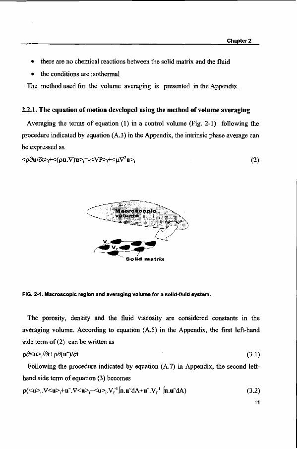
Averaging the terms of equation (1) in a control volume (Fig. 2-1) following the
procedure indicated by equation (A.3) in the Appendix, the intrinsic phase average can
be expressed as
<pôu/5t>i+<(pu.V)u>i=-<VP>i+<^V2u>i (2)
( M a c r o s c o p i c - -^ v o l u m e
S o l i d m a t r i x
FIG. 2-1. Macroscopic region and averaging volume for a solid-fluid system.
The porosity, density and the fluid viscosity are considered constants in the
averaging volume. According to equation (A.5) in the Appendix, the first left-hand
side term of (2) can be written as
p5<u>j/a+pô(u~)/at (3.1)
Following the procedure indicated by equation (A.7) in Appendix, the second left-
hand side term of equation (3) becomes
p(<u>j.V<u>i+u~.V<u>j+<u>i.Vf"1In.u~dA+u~.Vf
1 jn.u~dA) (3.2)
11
Forced fluid motion through openings and pores
and the right-hand side term
-V<P>i-Vf-1 JP~ dA+p. V2<u>j+(i Vf1 Jn.Vu~ dA (3.3)
At this point we need a representation for P~ and u~ as functions of the flow field in
order to obtain the closed form. For this, we will express the spatial deviation as a
linear function of some phase-averaged quantity, as used by Whitaker [10] in the
derivation of Darcy's law, and as supported by Slattery in previous work [6]. The
closure problem requires that the spatial deviation of the velocity and pressure be
represented in terms of intrinsic averaging velocity, which can be given by
u~=r. <u>j (4)
P~=uO.<u>, (5)
where T and O are tensors which relate the intrinsic phase average velocity to the
spatial deviation of velocity and pressure, respectively.
Substituting equations (4) and (5) in (3) yields
p5<u>/ôt+p5(r.<u>i)/ôt+p[<u>i.V<u>i+r.<u>i.V<u>i+
<u>i.<u>i.(Vf'In. rdA+VfT. In.rdA)]=-V<P>i+n V2<u>(+
+p.<u>i(Vf1 In.VrdA-Vf
1ll.OdA)+nV<u>i(Vf-1 JnT dA) (6)
where I is the unit tensor.
While intrinsic average pressure is used exclusively because it corresponds more
closely to the measured value, superficial average velocity is generally preferred in
practical situations. The spatial deviation of the velocity and pressure is much smaller
than the average value of the corresponding intrinsic phase. So T and O will be small
parameters. As <u>,»r<u>j and <u> are related by <u>| through <u>=s<u>j (see
Appendix), equation (6) becomes
(p/e)ô<u>/a+(p/£2)<u>.V<u>=-V<P>1+p.<u>.[(l/e)(Vf-1fn.VrdA-Vf-
||l.OdA)]-
p<u>.<u>.[(l/e2)(Vf-1[n.rdA)]+p.V<u>.[(l/8)Vf1 Jn.T dA]+(p/e)V2<u> (7)
Equation (7) is the key relation in this exercise. Compared with equation (1), in
addition to the terms accounting for the convective inertia effects {(p/e2)<u>.V<u>}
12
Chapter 2
and the viscous resistance of fluid flow {(u/s)V2<u>}, new terms
accounting for the effects of interaction between the fluid and the
matrix appear: {p<u>.<u>.[(l/e2)(Vf 'JnTdA)], ^V<u>.[(l/E)Vf-1Jn.rdA],
(a<u>.t(l/£)(Vf-1 fn.VrdA-Vf1 Jl.OdA)]}.
In the next section, the terms accounting for the effects of interaction between the
fluid and the matrix will be discussed, in order to clarify their physical meaning and
to present them in a more convenient and traditional way.
2.2.2 The range of validity of the motion equation
In order to complete the formulation of the motion equation developed in Section
2.2.1, the range of validity must be analysed. Therefore in this section two types of
medium will be analysed: a medium with poor fluid transmissivity and a medium with
high fluid transmissivity.
2.2.2-1 Medium with poor fluid transmissivity (the flow is considered to be incompressible [4])
If the flow is incompressible ( V<u>=0) and the volume of the solid matrix is larger
than the volume occupied by the fluid ((u/e)V2<u>»0 [11]), then the second left-
hand side term and the last right-hand side term of equation (7) can be discarded. This
allows us to write for a steady flow
p<u>.<u>.[(l/82)(Vf-1fn.rdA)]=-V<P>i+n<u>.[(l/e)(Vf
1 Jn.VrdA-Vf-' Jl.OdA)] (8)
Darcy domain
In the range of Darcy's law (Reynolds numbers not exceeding 1 [4]) the velocities
are very small. So, the squared fluid velocity term is negligible compared to the linear
fluid velocity term, and we obtain from equation (8)
H<u>.t(l/e)(Vf-1 jn.VrdA-Vf1 Il.OdA)]=V<P>i (9)
The term in brackets can be associated with the viscous resistance force due to
13
Forced fluid motion through openings and pores
momentum transfer at the matrix-fluid interface and is traditionally identified
as [10,11]
[(1/eXVf-1 jn.VrdA-Vf"1 Jl.OdA)]=-K-' (10)
where K is the permeability of the medium (m2).
Permeability represents the ability of the medium to transmit the fluid through it. In
accordance to kinetic gas theory [11], permeability is related to the reciprocal of the
collision frequency of diffusing particles against the solid matrix and the kinematic
fluid viscosity.
Forchheimer domain
In the Forchheimer domain [4] the pressure gradient is proportional to a linear term
of fluid velocity plus a squared velocity term (equation (8)). The term in brackets that
refers to the linear term is given by equation (10). The left-hand side term in brackets
relating to the pores' inertia effects is traditionally identified as [3,12]
[(l/^XVf-'Jn.rdA^YK-"2 (11)
where Y is a porous inertia factor.
2.2.2-2 Medium with high fluid transmissivity
A medium is very transmissive to fluid when its permeability is very high (K-»cc
and £«1 [11]). According to equations (10) and (11), the terms concerning the viscous
resistance force, brought about by the momentum transfer at the matrix-fluid
interface and the porous inertia effects can be discarded. The motion equation (7) will
be
pö<u>/at+p<u>.V<u>=-V<P>+p.V2<u>+p.V<u>.[(l/£)Vf-1 Jn.rdA] (12)
In accordance with equation (11) the last right side term in brackets of (12) can be
identified as YK"1/2. The permeability of a high fluid transmissivity medium is very
high (K —>oc) and YeK."2 —>0, that is, we recover the motion equation (1) valid for a
fluid volume element.
14
Chapter 2
2.2.3. Motion equation for a permeable medium
According to section 2.2.1 and 2.2.2 the motion equation for a permeable medium
(containing pores or openings) can be rewritten as
(p/8)5<u>/5t+(p/s2)<u>.V<u>=-V<P>r(u/K)<u>-pYK-1/2<u>.<u>+
uYeK-1/2V<u>+(n/s)V2<u> (13)
The advantages of the approach described by equation (13) when compared with the
existing literature [1-4] are
• one equation is sufficient to describe flows through media with pores up to
large openings instead of several equations,
• the approach was deduced without using empirical information.
The inertial factor Y was shown to be dependent on the porosity and a coefficient
cY, and can be obtained using the relationship [12,13]
Y=cYen (14)
The values usually employed are cy equal to 14.29xl0"2 or 4.36xl0'2 and n equal to
-1.5 or -2.12, for channels filled with packed beds [12] and for permeable screening
media [13], respectively.
Equation (13) is a non-linear differential equation and can be solved together with
mass and energy balance equations using numerical techniques within CFD. The
velocity, pressure and temperature throughout the flow field can be predicted.
Solving the transport equations numerically is difficult and in some engineering
applications the detail of CFD solutions is not required. For these applications it is
important to have a model which quantifies the phenomenon accurately and simply.
This will be the subject of the next section.
2.2.4. Simplified motion equation for pores and openings
In dealing with most of practical applications, an one-dimensional flow description
provides a good approximation [1-3]. Under this assumption equation (13) can be
written as
15
Forced fluid motion through openings and pores
(p/8)5<uj>/at+((j/K)<uj>+pYK-1/2<uj><uj>+Q<uj>=-a<Pj>i/ôj (15)
with
Q=[p8-2-Re1L(YsK-1/2+E-15/öj](a<uj>/öj)
where j represents the flow direction (perpendicular to the transmitting medium), Re
the Reynolds number and L a length dimension.
For porous media, according to Bear [4], du/cjj=0 and consequently
Q=0 (16)
In order to obtain Q for openings, consider a medium which has very high fluid
transmissivity (K - » « and second, third left-hand side terms can be discarded).
Assuming a steady flow, the resulting equation can be integrated along a streamline
and for any two points on this trajectory at distance H
0.5pA<u>2=A<P>+0.5pRe"1(L/H)A<u>2 (17)
with
A<u>2=<uH1>2-<uH2>
2
where um and uH2 are the velocity at two different points of the streamline.
To obtain a non-steady equation again, an integral (j9<u>/ôtdH=H 9<u>/9t) must be
added, becoming
5<u>/öt+0.5pCc"2<u>2/H=A<P>/H (18.1)
with
0.5pA<u>2=0.5pc,o<u>2 (18.2)
Cc={cl0[l-Re-'(L/H)]}-1/2 (18.3)
where H is the characteristic depth of the medium and c,0 a parameter accounting for
kinetic energy loss.
In accordance with equation (18.1), for openings, the parameter Q can be now
written as
Q=0.5pCc'2<u>/H (19)
The coefficient Cc is dependent on Re and on the characteristics of the opening. The
16
Chapter 2
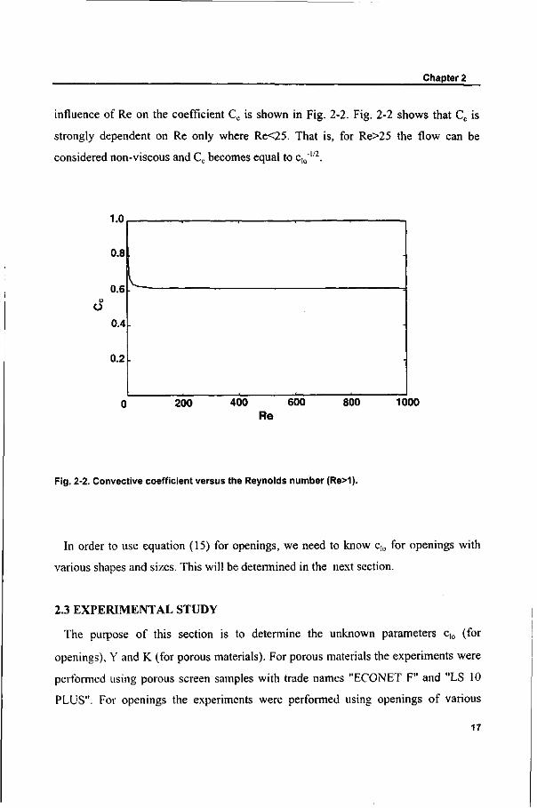
influence of Re on the coefficient Cc is shown in Fig. 2-2. Fig. 2-2 shows that Cc is
strongly dependent on Re only where Re<25. That is, for Re>25 the flow can be
considered non-viscous and Cc becomes equal to c,0""2.
Ü
Fig. 2-2. Convective coefficient versus the Reynolds number (Re>1).
In order to use equation (15) for openings, we need to know c,0 for openings with
various shapes and sizes. This will be determined in the next section.
2.3 EXPERIMENTAL STUDY
The purpose of this section is to determine the unknown parameters clo (for
openings), Y and K (for porous materials). For porous materials the experiments were
performed using porous screen samples with trade names "ECONET F" and "LS 10
PLUS". For openings the experiments were performed using openings of various
17
Forced fluid motion through openings and pores
shapes and sizes. In both experiments, the samples were subjected to several air flows,
causing a constant pressure drop between the sample sides (DC-pressurization
method [13]).
2.3.1. Description of experiments
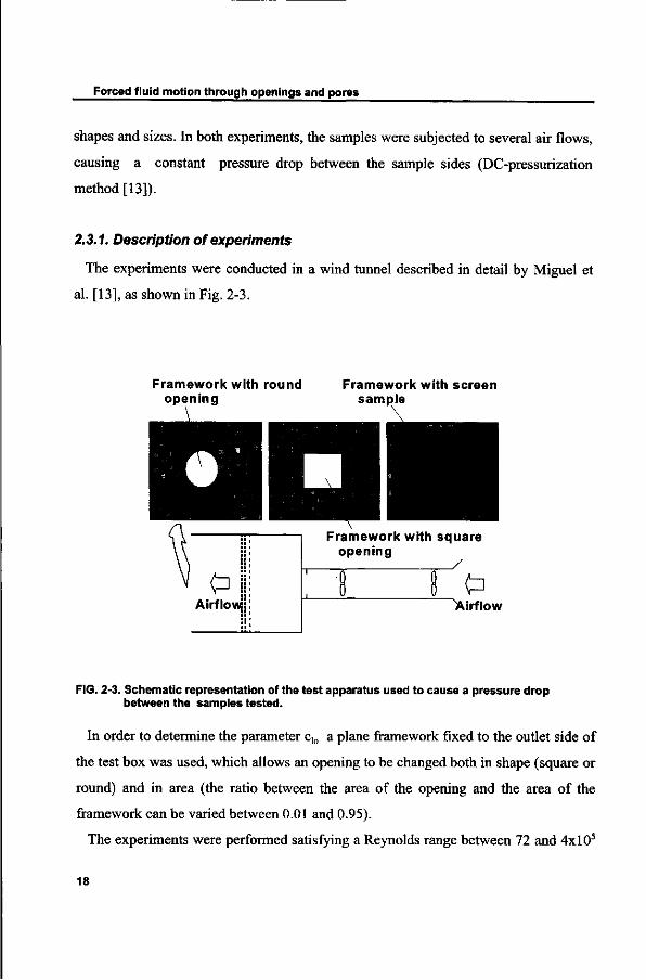
The experiments were conducted in a wind tunnel described in detail by Miguel et
al. [13], as shown in Fig. 2-3.
Framework with round opening
Framework with screen sample
Framework with square opening
/
Airflow
FIG. 2-3. Schematic representation of the test apparatus used to cause a pressure drop between the samples tested.
In order to determine the parameter clo a plane framework fixed to the outlet side of
the test box was used, which allows an opening to be changed both in shape (square or
round) and in area (the ratio between the area of the opening and the area of the
framework can be varied between 0.01 and 0.95).
The experiments were performed satisfying a Reynolds range between 72 and 4xl05
18
Chapter 2
(excluding the influence of viscous effects).
In order to determine the parameters Y and K, the test screens were fixed to the
outlet side of the test box using a wooden frame, which prevents air leakage. The
experiments were performed satisfying a Reynolds range between 0.7 and 97.
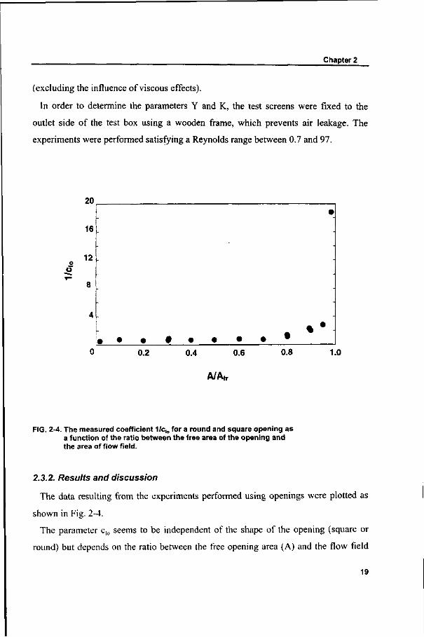
A/Afr
FIG. 2-4. The measured coefficient 1/clo for a round and square opening as a function of the ratio between the free area of the opening and the area of flow field.
2.3.2. Results and discussion
The data resulting from the experiments performed using openings were plotted as
shown in Fig. 2-4.
The parameter cb seems to be independent of the shape of the opening (square or
round) but depends on the ratio between the free opening area (A) and the flow field
19
Forced fluid motion through openings and pores
area (Afr). It is in full agreement with the equation
c,o={2.7-0.04203exp[3.7(A/Afr)1/2]}
{l-[2.7-0.04203 exp[3.7(A/Afr)1/2]] (A/Afr)
25}1/2 (20)
Substituting equation (20) in (18.3) provides
Cc-2=[1-Re-'(L/H)] {2.7-0.04203 exp[3.7(A/Afr)
1/2]}
{l-[2.7-0.04203 exp[3.7(A/Afr)1/2]](A/Afr)
25}1/2 (21)
Frame
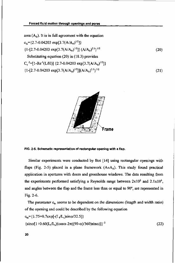
FIG. 2-5. Schematic representation of rectangular opening with a flap.
Similar experiments were conducted by Bot [14] using rectangular openings with
flaps (Fig. 2-5) placed in a plane framework (A«Afr). This study found practical
application in apertures with doors and greenhouse windows. The data resulting from
the experiments performed satisfying a Reynolds range between 2xl02 and 2.1xl04,
and angles between the flap and the frame less than or equal to 90°, are represented in
Fig. 2-6.
The parameter c,0 seems to be dependent on the dimensions (length and width ratio)
of the opening and could be described by the following equation
clo={1.75+0.7exp[-(L,/Ls)sina/32.5]}
{sina[ 1 +0.60(L,/Ls)(cosa-27t((90-a)/360)sina)]} "2 (22)
20
Chapter 2
and
O / H {1.75+0.7exp[-(L/Ls)sina/32.5]} {sina[l+0.60(L,/Ls)
(cosa-27i((90-a)/360)sina)]}-2 [l-Re''(Ls/H)]} (23)
where a is the opening angle between the flap and the frame, L, the larger length of
the opening and Ls the smaller length of the opening.
20 40 60
OPENING ANGLE (°)
80
FIG. 2-6. The measured coefficient 1/c,„ for a rectangular opening as a function of opening angle between the flap and the frame.
According to equation (20), for A=Alr there are no flow obstructions and c,0 is zero
(Cc":=0), i.e., pressure drop is equal to zero. Therefore, according to equations (20) and
(22), for a non-viscous flow through a round or square opening in a large framework
(A/Atv~0), and for an opening with opening angle of 90°, the coefficient Cc achieves
values close to 0.60 and 0.63, respectively. These values are close to the value usually
found for the so-called "discharge coefficient" in the literature (0.61).
21
Forced fluid motion through openings and pores
14
TO a . OL O oc Q LU DC 3 (/) CO Ui cc a.
12
10
ö
6
4
2 ^£P
o o ÖB)
c» ~-OD OST
tf^ J-1^
<*b
»
«f* .
-
.
* • - "
1 2
VELOCITY (m/s)
FIG. 2-7. Pressure drop as a function of the velocity for a porous screen trade name "ECONET F".
120
0.1 0.2
VELOCITY (m/s)
FIG. 2-8. Pressure drop as a function of the velocity for a porous screen trade name "LS 10 PLUS".
22
Chapter 2
The data resulting from the experiments performed using porous screen samples
were plotted as shown in Figs. 2-7 and 2-8.
The parameters Y and K are obtained fitting the experimental data with the
Forchheimer equation. The permeabilities obtained for screen ECONETF and LS 10
PLUS were 6.51xl009 m2 and 6.79xl0_u m2, and parameter Y equal to 0.457 and
7.18, respectively. The porosities can then be found using equation (14) and were 0.09
and 0.33, respectively.
Equation (15) together with equations (16), (21) and (23) form a simplified
mathematical model to describe one-dimensional forced fluid motion through pores
and openings.
2.4 CONCLUSIONS
This paper describes some physical aspects of forced convection through permeable
media. The results described above show that, for forced convection, one theory seems
to be sufficient to describe flow phenomena through porous media and through
non-porous media (gaps, cracks, doors, windows).
The approach developed in this study enables the air infiltration in enclosed spaces
to be analysed. We describe this application elsewhere [15].
2.5 REFERENCES
[1] Allard F. and Utsumi Y. 1992. Airflow through large openings, Energy and
Buildings 26, 133-145
[2] Baker P. H., Sharpies S. and Ward I. C. 1987. Air flow through cracks, Build.
and Environment 22, 293-304
[3] Forchheimer P. 1901. Wasserbewegung durch boden, Z. Ver. Deutsch. 45, 1782-
1788 [in German]
23
Forced fluid motion through openings and pores
[4] Bear J. 1972. Dynamics of fluids in porous media, American Elsevier
Environmental Sciences Series, New York, USA
[5] Gray W. G. 1975. A derivation of the equations for multiphase transport, Chem.
Engng. Sei. 30, 229-233
(6] Slattery J. C. 1967. Flow of viscoelastic fluids through porous media, AIChE
Journal 13, 1066-1071
[7] Howes F. A. and Whitaker S. 1985. The spatial averaging theorem revisited,
Chem. Engng. Sei. 40, 1387-1392
[8] Quintard M. and Whitaker S. 1994. Transport in ordered and disordered porous
media II: Generalized volume averaging, Transport in porous media 14, 179-206
[9] Quintard M. and Whitaker S. 1987. Écoulement monophasique en milieu
poreux: Effet des hétérogénéités locales, J. Méc. Théor. Appl. 6, 691-726
[10] Whitaker S. 1986. Flow in porous media I: A theoretical deviation of Darcy's
law, Transport in Porous media 1, 3-25
[11] Lebon G. and Cloot A. 1986. A thermodynamical modelling of fluid flows
through porous media: application to natural convection. Int. J. Heat Mass Transfer,
29,381-390
[12] Ergun S. 1952. Fluid flow through packed columns, Chemical Engineering
Progress 48, 89-94
[13] Miguel A. F., van de Braak N. J., Silva A. M. and Bot G. P. A. 1997.
Analysis of the airflow characteristics of greenhouse screens, J. Agr. Eng. Research
67,105-112.
[14] Bot G. P. A. 1983. Greenhouse climate: from physical processes to a dynamic
model, Ph.D. Dissertation, Agricultural University of Wageningen, The Netherlands
[15] Miguel A. F., van de Braak N. J., Silva A. M. and Bot G. P. A. 1998.
Analysis of air exchange and internai pressures in enclosures induced by fluctuating
outside pressures, Building and Environment (in press)
24
Chapter 2
2.6 APPENDIX
Basic formulation of the method of volume averaging
Consider a homogeneous system whose averaging volume, represented in Fig. 2-1,
is invariant with respect to time and space. For a two-phase system (solid matrix and
fluid) the averaging volume is defined as
V=Vs+Vf (A.l)
where Vs and Vf represent the volume of the solid and fluid contained within the
averaging volume, respectively.
The fluid porosity e is given by
£=V/V (A.2)
The porosity represents the volume fraction of fluid contained within the averaging
volume of the medium and it is between 0 and 1 (0<e<l). Specifically for one opening
it is 1 (e=l, all open volume is filled with fluid).
The average of a local quantity A (fluid velocity, fluid pressure) in the averaging
volume, can be formulated in terms of superficial (external) phase average or intrinsic
(internal) phase average. The intrinsic (internal) phase average is defined as
<A>,=Vf-1jAdV (A.3-1)
and the superficial (external) phase average as
<A>=V-'jAdV (A.3-2)
where <A> is the superficial phase average of local quantity A and <A> the intrinsic
phase average of local quantity A.
These two averages are related by the porosity according to
<A>=s <A>i (A.4)
The local values of the quantity A can also be related to the phase averages
according to [5]
A=<A>j+A~ (A.5)
where A~ is the spatial deviation of A compared to <A>j.
25
Forced fluid motion through openings and pores
In the analysis of equations governing transport phenomena in porous media it is
usual to interchange differentiation and integration in order to express the quantity in
terms of intrinsic phase average. This will be done by means of the spatial averaging
theorem [6,7]. This theorem can be written in vector form as
<V.A>i=V.<A>, + V"1 Jn.AdA (A.6)
where n is a unit vector and A the interfacial area contained within the averaging
volume.
Substitution of equation (A.5) in equation (A.6) gives
<V.A>j=V.<A>i + Vf1 Jn^A^dA+Vf1 jn.A~dA (A.7)
As the system under consideration is homogeneous, <A>S can be treated as a
constant, and consequently the area integral becomes
Vf-' Jn.<A>i dAK^'V"1 IndA).<A>i (A.8)
The integral in parenthesis is related to the structure of the volume studied and can
be expressed by [8]
s-'V' jndA=-Ve/E (A.9)
which can easily be proved to be zero for a homogeneous system.
If the system studied is heterogeneous, that is, it is characterised by more than one
length scale, we will need to use a large-scale averaging [9]. Heterogeneous systems
are beyond the scope of this study.
2.7 NOMENCLATURE
A area [m2]
Cc coefficient accounting for convective inertia and viscous effects
clo parameter accounting for kinetic energy loss
H characteristic depth [m]
K permeability [m2]
L length dimension [m]
26

Chapter 2
P pressure [Pa]
Re Reynolds number
t time [s]
û velocity [ms"1]
V volume [m3]
Y inertial factor
Greek symbols
a opening angle between the flap and the frame [°]
s porosity
A local general quantity likes velocity or pressure
<A> superficial (external) phase average of quantity A
<A>j intrinsic (internal) phase average of quantity A
p. dynamic viscosity [Pa s]
p density [kg m"3]
Subscripts
f fluid
fr flow field
i intrinsic
27
28
3. Analysis of air exchange induced by fluctuating external pressures in enclosures +
Abstract: A new approach using the equations of mass conservation and motion, and
the state equation of gases, is proposed to characterise air infiltrations induced by
fluctuating pressures. The approach is applied to a two-zone enclosure with openings
and pores. Experimental data obtained for the purpose of testing the validity of the
approach are found to agree well with the predicted values.
3.1 INTRODUCTION
Air infiltration in enclosures is the main process, which affects the mass and energy
balance inside the enclosure and consequently the indoor climate [1]. The continuing
interest in this topic is based on the lack of a comprehensive and satisfactory theory,
despite much important work and a great number of studies that has been done [2,3].
Pressure due to wind is one of the main driving forces in the study of air infiltration
in enclosures. Wind velocity fluctuates and therefore induces wind pressures (with a
mean component and a fluctuating component) which influence pressure differences
between the inside and outside of the enclosures.
The internal pressure in any enclosure is controlled by the wind pressure and by the
characteristics of the enclosure envelope [4,5]. The nature of response of internal
pressure due to the wind was first studied by Euteneuer [6]. However, he neglected the
inertia effect of the airflow entering the opening. Inspired by the classical Helmholtz
resonator model, Holmes [7] and Liu and Saathoff [8] studied the transient response of
internal pressure fluctuations in a constant volume enclosure with one large opening
using a second-order non-linear differential equation. Recently, Dewsbury [9]
presented a model, which includes variation of the enclosure volume. Liu and Rhee
[10] made an experimental study of the nature of the wind-induced Helmholtz
oscillation of air pressure in buildings. They demonstrated that the tendency to
' Building and Environment (in press)
Air exchange induced by fluctuating pressures
resonance increases concomitantly with a window area increasing relative to the
volume of the building.
The differences in internal and external pressure induce air infiltrations in
enclosures. The models available in literature describe the air infiltrations through
narrow openings (pores, gaps, cracks) [11,12] and through large openings (windows,
doors) [13,14]. For narrow openings the majority are based on empirical equations and
for large openings on Bernoulli's equation. The empirical parameters in these
equations are determined by performing experiments in which air is forced through the
enclosure envelope, producing a constant pressure difference between inside and
outside (DC-pressurization method [15]) or producing a sinusoidal pressure
difference (AC-pressurization method [9,16,17]). The parameters are obtained by
fitting the experimental data with appropriate equations.
The purpose of this paper is to present a coherent mathematical model, based on
principles of physics, studying airflow in enclosures with openings and pores induced
by fluctuating external pressures. The applicability of the model is illustrated through
the study of air exchanges in a two-zone enclosure with openings and pores.
3.2 MATHEMATICAL FORMULATION
3.2.1. General description of the model
Consider an enclosure of volume Ve, exchanging air with the outside, through one
opening with a large free area, or through a structure with narrow openings or pores of
area A. Under the assumptions that
• the air within the enclosure is an ideal gas and compressible
• the air exchange with the exterior is unidimensional
we can write
The equation of mass conservation for air within the enclosure
dM/dt=Apu (1.1)
30
Chapter 3
or
pdV/dt+Vdp/dt=A p u (1.2)
with
v=ve-snvn
where u represents the air velocity through the infiltrations, M total mass of air in the
enclosure, p the density of air in the enclosure, A the area of infiltrations, t the time, V
the total volume of air in the enclosure, Ve the volume of enclosure and Vn the volume
of objects within the enclosure.
Usually the enclosure envelope is considered to be rigid and not to deform
(dVe/dt=0). In reality, however, the roof and walls deform to an extent that depends on
the magnitude of pressure exerted, influencing the airflow through the enclosure
envelope. Bearing in mind the behaviour of elastic materials, the enclosure
deformation can be simply calculated assuming
(Ve-Vem)/Vem=T! ( p -p j (2)
where Vem represents the mean volume of the enclosure, p the pressure, pm the mean
pressure and r\ the enclosure flexibility coefficient.
Substituting (2) in (1.2) yields
(Vem-InVn)p,dp/dt=A u+SndVn/dt-r)Vemdp/dt (3)
This equation indicates how the density of air within the enclosure is related to the
airflow through the infiltrations, the enclosure flexibility and the volume change of
objects within the enclosure.
The j-direction motion equation for air through openings and pores [18]
(p/s)au/ôt+p.K",u+pq|u|u=ôp/5j (4)
with
q=(4.36xl0-28-212K1/2+0.5Cc-2/H)
where e is the porosity [18], K the permeability [18], \x. the fluid dynamic viscosity, p
the pressure, H the characteristic depth of the medium and Cc a coefficient accounting
31
Air exchange induced by fluctuating pressures
for convective inertia and viscous effects.
For a porous medium [18]
Cc-2=0 (5.1)
for round and square openings [18]
CVMl-Re-'CL/H)] {2.7-0.04203 exp[3.7(A/Afr)1/2]}
{1-[2.7-0.04203 exp[3.7(A/Afr)1/2]](A/Afr)
25}"2 (5.2)
and for rectangular openings covered with movable flaps [18]
C;2={{1.75+0.7exp[-(L,/Ls)sina/32.5]} {sina[l+0.60(L,/Ls)
(cosa-27t((90-a)/360)sina)]}-2 [ l -Re '^ /H)]} (5.3)
where a is the opening angle between the flap and the frame, Re the Reynolds
number, Afr the flow field area, L, the larger length of the opening and Ls the smaller
length of the opening.
The equation of state for air within the enclosure
p=PRgT (6)
where T represents the absolute temperature and Rg the specific gas constant.
For a polytropic expansion or compression of ideal gas with constant heat capacity,
equation (6) can be rewritten as
pp"p=constant (7)
where ß is 1.4 for isentropic air expansion/compression and 1.0 for isothermal air
expansion/compression.
3.2.2. Fluctuating pressure inside an enclosure where air is exchanged with the outside through one opening with a large free area or through a structure with narrow openings or pores
Pressure within an enclosure with compressible air
When pressure is applied to the air inside the enclosure, this is compressed and its
32
Chapter 3
density changes. Consider a polytropic compression/expansion of the air within the
enclosure. Substituting equation (7) in (3) gives, after integration,
(Vem-ZnVnm)ß-1(Ap/p)+T1Vem Ap=jA u dt+Zn(Vn-Vn J (8)
with
Ap=p,=p-pm
where Vnm represents the mean volume of objects inside the enclosure and Ap or p; the
pressure change within the enclosure.
Considering a small pressure change (P(«p), equation (8) can be conveniently
rewritten as
[(Vem-EnVnJ+ßpmTiVem]p1=ßpmK u dt+ßpmIn(Vn-Vnm) (9)
Equations (8) and (9) describe the pressure change inside the enclosure which is the
fluctuating component of internal pressure.
Transient response of internal air pressure
The internal pressure also changes in response to the fluctuations occurring in the
external pressure. The transient response of internal pressure can be easily obtained by
substituting equations (3) and (7) in (4). The resulting equation is quite long and may
by summarised as
a1d2p/dt2+a2|dp/dt|dp/dt+a3dp/dt-a4d(ZnVn)/dt|dp/dt|-a5d
2(SnVn)/dt2+
a6d(2nVn)/dt+p=pext (10)
with
a=a(p,ß ,pm,pm,r|,H,A,n,K,q,Vem,£nVn, SnVnm)
where pm represents the mean fluid density and pext the external pressure.
Since the volume of objects inside the enclosure does not deform, equation (10) can
be simplified to
a, d2p/dt2+a2|dp/dt|dp/dt+a3dp/dt+AH1p=AH-1pext (11)
with
a1=pme-,t(Vein-EnVninXßpJ-,+tiVeJ
33
Air exchange induced by fluctuating pressures
a2=PmqA-2[(Vem-InVnm)2(ppJ-2+2îiVem(Vem-SnVnm)(PpJ-'+(TiVem)2]
a3=^K1[(Vem-EnVnJ(ßpm)-1+TiVem]-pm(Vem-InVnJ(sßpm2)-1
Equations (10) and (11) are second-order non-linear differential equations and the
following situations can occur:
• for an enclosure with an opening with a relatively large free area (K-»oc =>
|aK"' and 4.36xl0"2e"212K",/2 are negligible compared to 0.5CC"2/H), equations
(10) and (11) present two forms of solution:
a) for A«(Vem-E„Vnm) or A«r|Vem the second order term is important and we
have a damped resonance equation (gradual decay)
b) for A»(Vem-£nVnm) and A»r|Vem the second order term is very small and we
have an oscillatory equation with very little damping
• for an enclosure with narrow openings and pores ((iKr'wO, q»0), equations
(10) and (11) are always damped resonance equations.
Our finding that the larger the area of the opening in relation to the enclosure
volume, the greater the tendency to resonance, is supported by the observations of Liu
andRhee[10].
As we mentioned earlier, Holmes [7], Liu and Saathoff [8] and Dewsbury [9],
presented models to study the transient response of internal pressure in enclosures
with compressible air. Although the models presented by these authors also contain
second-order non-linear differential equations and describe internal pressures in
enclosures with large openings, they fail to describe internal pressures in enclosures
with narrow openings and pores. The model presented here also differs from the
models of Holmes [7], and Liu and Saathoff [8] in the following aspects
• it accounts for the flexibility of the enclosure envelope
• it accounts for volume changes of objects within the enclosure.
Equations (10) and (11) can not only be used to describe the change in internal
pressure due to sudden opening or breaking of an aperture (window, door, etc.) under
external pressure but also to obtain parameters r\, K, Cc, A and H. These parameters
34
Chapter 3
can be obtained accurately using the experimental procedure described by Dewsbury
[9], and will cause little impact on the indoor environment.
Oscillation of internal pressure in enclosures with openings and pores
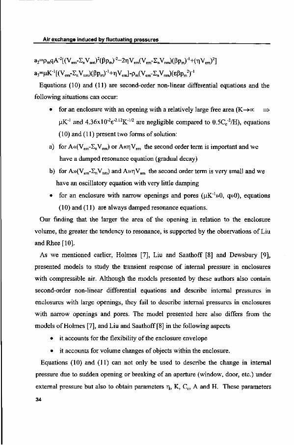
The solution of equation (11) can be compared with the models presented by Liu and
Saathoff [8] and Dewsbury [9], by means of a numerical study. This comparison
considers the hypothetical case of an enclosure (rigid volume of 200 m3, r|=0 Pa"1)
with one window (area of 2x2 m2). The example also uses the following values: a
stagnation pressure of 500 Pa, the parameter ß equal to 1.4 (isentropic
expansion/compression), the leakage coefficient 0.6 and the leakage exponent 2, both
in Dewsbury equation. We used the atmospheric pressure as the initial internal
pressure, and the stagnation pressure as the external pressure at the opening. The
result is presented as a dimensionless quantity rp, which represents the ratio between
the pressure in the enclosure and the stagnation pressure, as shown in Fig. 3-1.
From Fig. 3-1, it can be concluded that the profile of the solutions is oscillatory and
exhibits damping. The maximum amplitude oscillation (first cycle) occurs in equation
(11). A difference in amplitude of about 4% is obtained by using the Liu and Saathoff
equation, and of 1.4% by using the Dewsbury equation.
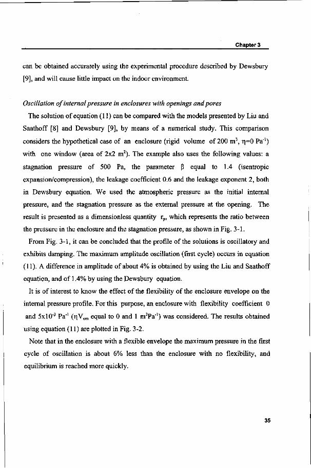
It is of interest to know the effect of the flexibility of the enclosure envelope on the
internal pressure profile. For this purpose, an enclosure with flexibility coefficient 0
and 5xlO"3 Pa"1 (r|Vcm equal to 0 and 1 m3Pa') was considered. The results obtained
using equation (11) are plotted in Fig. 3-2.
Note that in the enclosure with a flexible envelope the maximum pressure in the first
cycle of oscillation is about 6% less than the enclosure with no flexibility, and
equilibrium is reached more quickly.
35
Air exchange induced by fluctuating pressures
£ 1
FIG. 3-1. Comparison of the solution presented by Liu and Saathoff [8] (-.-), by Dewsbury [9] (--) with the solution of equation (11) (—) for the internal pressure change due to sudden opening or breakage of an aperture.
.o. 1
0.2 0.4 0.6
TIME (s)
0.8 1.0
FIG. 3-2. Internal pressure change for an enclosure with flexible envelope (--) and with rigid envelope (—).
36
Chapter 3
1.2
0.8
0.4
- ƒ
" /
-// /
-.,
/'
/
'''
,*-*,
.•"'"*-''
.—. ••-J"-'*
,-—-. , ^
—1—-—-"—
.
—
-
0.1 0.2 0.3
TIME (s)
0.4
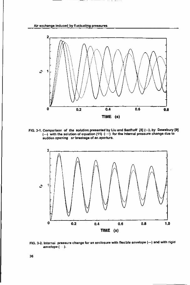
FIG. 3-3. Internal pressure change for enclosure with pores and narrow openings (K=107 m2: E=0.25 (—) and e=0.75 (...); K=103 m2: E=0.25 (---) and s=0.75 (-.-)).
To illustrate the nature of the solutions of equation ( 11 ) for narrow openings and for
pores (beyond the range of the models available in the literature [7-9]), structures of
permeability K=10'3m2 and K=10'7m2 (porosity 8=0.25 and e=0.75) were considered.
The values for the remaining quantities, and the assumptions made are the same as for
the example included in Fig. 3-1, and the result is presented in Fig. 3-3.
Fig. 3-3 shows that, for the structure with permeability of 10"3m2, the maximum
value of the internal pressure coefficient (first cycle of oscillation) is about 1.242 for
structure of porosity 0.75 (exceeding the internal pressure by about 24.2%) and 1.025
for structure of porosity 0.25 (exceeding the internal pressure by about 2.5%). For the
structure with permeability of 10"7m\ the internal pressure is exceeded by 1.6% and
37
Air exchange induced by fluctuating pressures
0.2% for structures of porosity 0.75 and 0.25, respectively. In both situations the
internal pressure is strongly damped and the equilibrium is reached almost
immediately.
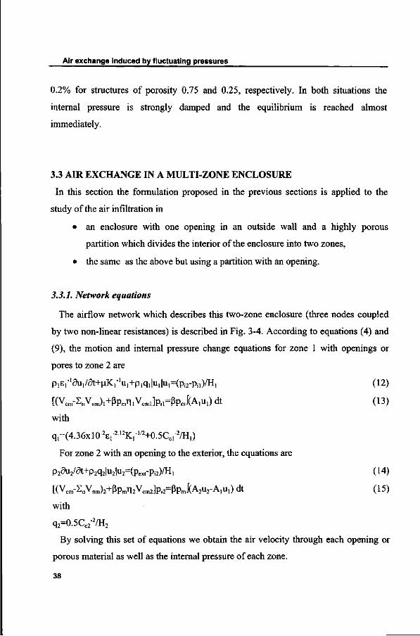
3.3 AIR EXCHANGE IN A MULTI-ZONE ENCLOSURE
In this section the formulation proposed in the previous sections is applied to the
study of the air infiltration in
• an enclosure with one opening in an outside wall and a highly porous
partition which divides the interior of the enclosure into two zones,
• the same as the above but using a partition with an opening.
3.3.1. Network equations
The airflow network which describes this two-zone enclosure (three nodes coupled
by two non-linear resistances) is described in Fig. 3-4. According to equations (4) and
(9), the motion and internal pressure change equations for zone 1 with openings or
pores to zone 2 are
Pi8,-1au1/a+p.Kr1u1+p1q,|u1|u1=(pi2-pil)/H1 (12)
[(Ven,-EnVran)I+ßPinTi1Venil]pil=ßpnii[AIuI) dt (13)
with
q,=(4.36xl0-2eI-212K1-
1/2+0.5Ccl-2/H1)
For zone 2 with an opening to the exterior, the equations are
p2du2/5t+p2q2|u2|u2=(pext-pi2)/H, (14)
[(Vem-InVnm)2+ßpmii2Vem2]pi2=ßpmI(A2u2-A1u1) dt (15)
with
q2=0.5Cc2"2/H2
By solving this set of equations we obtain the air velocity through each opening or
porous material as well as the internal pressure of each zone.
38
Chapter 3
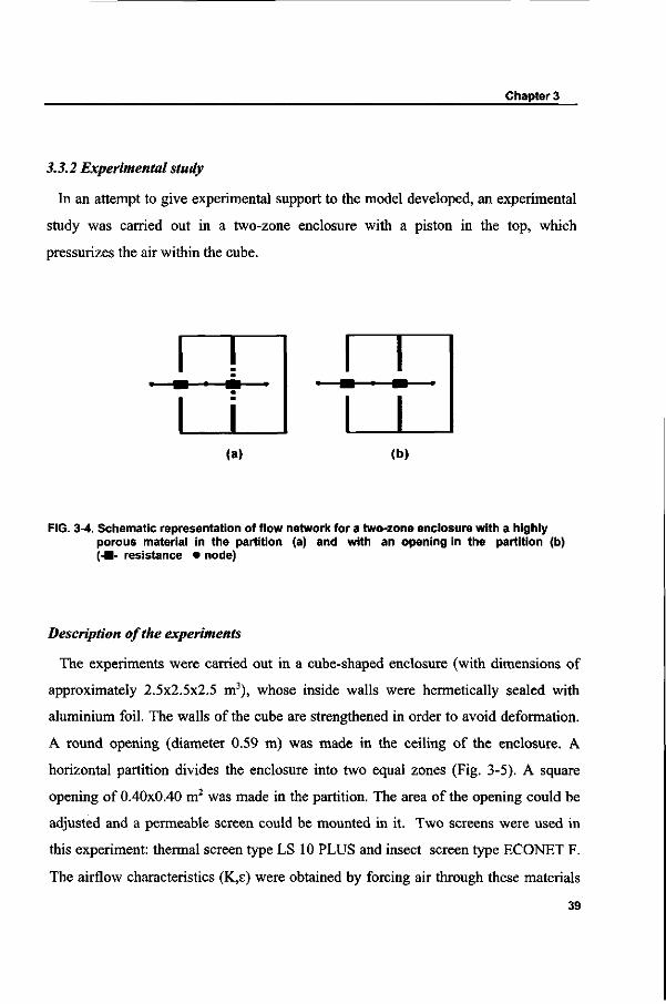
3.3.2 Experimental study
In an attempt to give experimental support to the model developed, an experimental
study was carried out in a two-zone enclosure with a piston in the top, which
pressurizes the air within the cube.
n m n
(a) (b)
FIG. 3-4. Schematic representation of flow network for a two-zone enclosure with a highly porous material in the partition (a) and with an opening in the partition (b) (-•- resistance • node)
Description of the experiments
The experiments were carried out in a cube-shaped enclosure (with dimensions of
approximately 2.5x2.5x2.5 m3), whose inside walls were hermetically sealed with
aluminium foil. The walls of the cube are strengthened in order to avoid deformation.
A round opening (diameter 0.59 m) was made in the ceiling of the enclosure. A
horizontal partition divides the enclosure into two equal zones (Fig. 3-5). A square
opening of 0.40x0.40 m2 was made in the partition. The area of the opening could be
adjusted and a permeable screen could be mounted in it. Two screens were used in
this experiment: thermal screen type LS 10 PLUS and insect screen type ECONET F.
The airflow characteristics (K,s) were obtained by forcing air through these materials
39
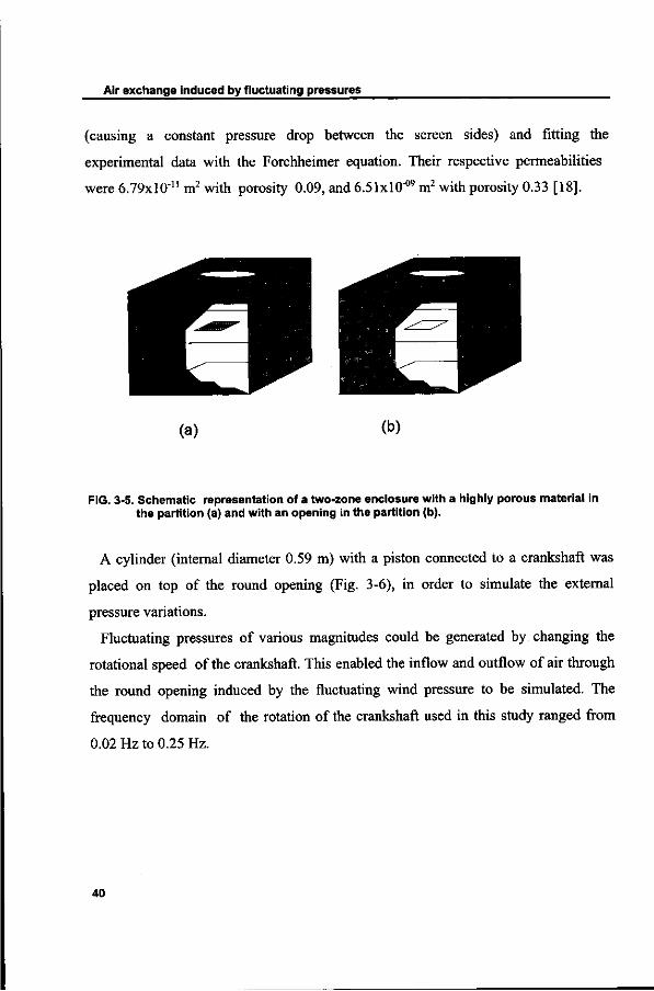
Air exchange induced by fluctuating pressures
(causing a constant pressure drop between the screen sides) and fitting the
experimental data with the Forchheimer equation. Their respective permeabilities
were 6 .79xl0u m2 with porosity 0.09, and 6.51X10"09 m2 with porosity 0.33 [18].
(a) (b)
FIG. 3-5. Schematic representation of a two-zone enclosure with a highly porous material in the partition (a) and with an opening in the partition (b).
A cylinder (internal diameter 0.59 m) with a piston connected to a crankshaft was
placed on top of the round opening (Fig. 3-6), in order to simulate the external
pressure variations.
Fluctuating pressures of various magnitudes could be generated by changing the
rotational speed of the crankshaft. This enabled the inflow and outflow of air through
the round opening induced by the fluctuating wind pressure to be simulated. The
frequency domain of the rotation of the crankshaft used in this study ranged from
0.02 Hz to 0.25 Hz.
40
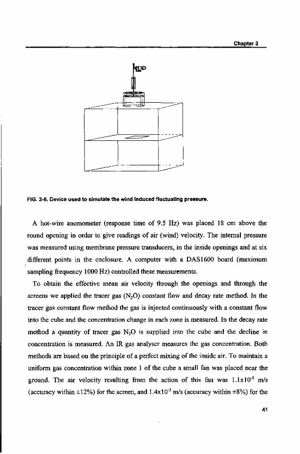
Chapter 3
FIG. 3-6. Device used to simulate the wind induced fluctuating pressure.
A hot-wire anemometer (response time of 9.5 Hz) was placed 18 cm above the
round opening in order to give readings of air (wind) velocity. The internal pressure
was measured using membrane pressure transducers, in the inside openings and at six
different points in the enclosure. A computer with a DAS 1600 board (maximum
sampling frequency 1000 Hz) controlled these measurements.
To obtain the effective mean air velocity through the openings and through the
screens we applied the tracer gas (N20) constant flow and decay rate method. In the
tracer gas constant flow method the gas is injected continuously with a constant flow
into the cube and the concentration change in each zone is measured. In the decay rate
method a quantity of tracer gas N 20 is supplied into the cube and the decline in
concentration is measured. An IR gas analyser measures the gas concentration. Both
methods are based on the principle of a perfect mixing of the inside air. To maintain a
uniform gas concentration within zone 1 of the cube a small fan was placed near the
ground. The air velocity resulting from the action of this fan was l.lxlO"5 m/s
(accuracy within ±12%) for the screen, and 1.4xl0"3 m/s (accuracy within ±8%) for the
41
Air exchange induced by fluctuating pressures
opening. In zone 2 no fans were used.
Results and discussion
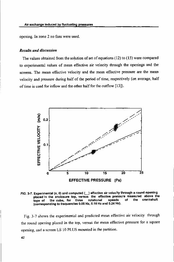
The values obtained from the solution of set of equations (12) to (15) were compared
to experimental values of mean effective air velocity through the openings and the
screens. The mean effective velocity and the mean effective pressure are the mean
velocity and pressure during half of the period of time, respectively (on average, half
of time is used for inflow and the other half for the outflow [13]).
(A
1 >-i-Ô O _! > 111 > o UJ u. liai
0.2
0.1
y. /;-'
/ < - ' ' •
Jw ^ < * ' ' ^ ^
S-' ^ ^ ^ ^ ^
S-' ^^^ S'' Jw
^ \ ^ ^ /C^ s£^
0 5 10 15 20 25
EFFECTIVE PRESSURE (Pa)
FIG. 3-7. Experimental (x, 0) and computed ( ) effective air velocity through a round opening placed in the enclosure top, versus the effective pressure measured above the tope of the cube, for three rotational speeds of the crankshaft (corresponding to frequencies 0.08 Hz, 0.16 Hz and 0.24 Hz).
Fig. 3-7 shows the experimental and predicted mean effective air velocity through
the round opening placed in the top, versus the mean effective pressure for a square
opening, and a screen LS 10 PLUS mounted in the partition.
42
Chapter 3
The mean effective air velocity through the top opening in the case of the square
opening in the partition is larger than when the screen is in the partition. This is
because the inside air volume available for pressurization or depressurization is larger
in the case of the square opening than in the case of the screen.
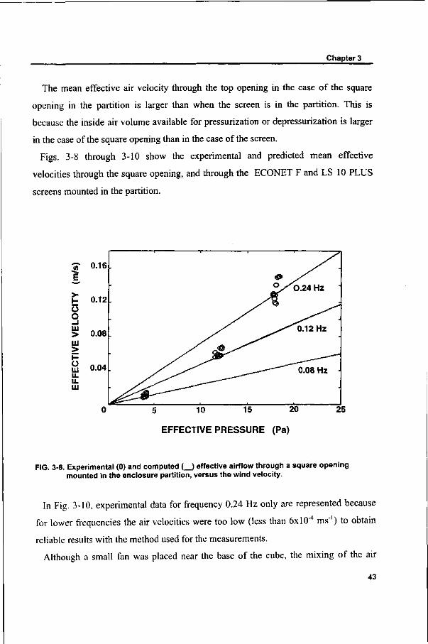
Figs. 3-8 through 3-10 show the experimental and predicted mean effective
velocities through the square opening, and through the ECONET F and LS 10 PLUS
screens mounted in the partition.
'T) E
• " • '
> H O O - l UI > UI > H O UI u. IL UI
0.16
0.12
0.08
0.04 0.08 Hz
5 10 15 20 25
EFFECTIVE PRESSURE (Pa)
FIG. 3-8. Experimental (0) and computed (_) effective airflow through a square opening mounted in the enclosure partition, versus the wind velocity.
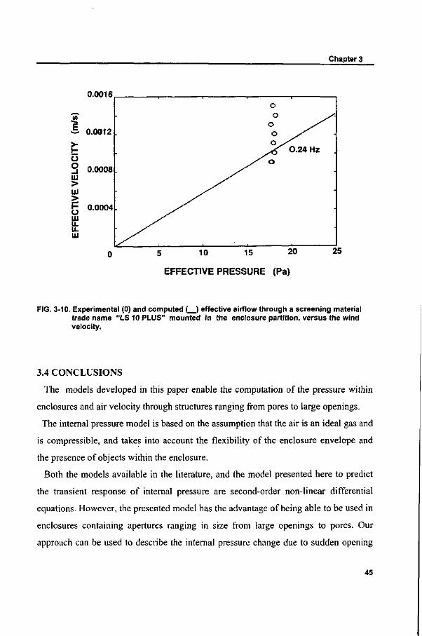
In Fig. 3-10, experimental data for frequency 0.24 Hz only are represented because
for lower frequencies the air velocities were too low (less than 6xl0"4 ms'1) to obtain
reliable results with the method used for the measurements.
Although a small fan was placed near the base of the cube, the mixing of the air
43
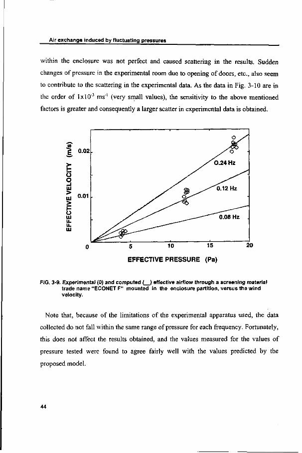
Air exchange induced by fluctuating pressures
within the enclosure was not perfect and caused scattering in the results. Sudden
changes of pressure in the experimental room due to opening of doors, etc., also seem
to contribute to the scattering in the experimental data. As the data in Fig. 3-10 are in
the order of lxlO"3 ms"' (very small values), the sensitivity to the above mentioned
factors is greater and consequently a larger scatter in experimental data is obtained.
5 10 15
EFFECTIVE PRESSURE (Pa)
FIG. 3-9. Experimental (0) and computed ( ) effective airflow through a screening material trade name "ECONET F" mounted in the enclosure partition, versus the wind velocity.
Note that, because of the limitations of the experimental apparatus used, the data
collected do not fall within the same range of pressure for each frequency. Fortunately,
this does not affect the results obtained, and the values measured for the values of
pressure tested were found to agree fairly well with the values predicted by the
proposed model.
44
Chapter 3
0.0016
•§- 0.0012
O O _i UJ > UI > F o ui u. liai
0.0008
0.0004.
5 10 15 20
EFFECTIVE PRESSURE (Pa)
FIG. 3-10. Experimental (0) and computed ( ) effective airflow through a screening material trade name "LS 10 PLUS" mounted in the enclosure partition, versus the wind velocity.
3.4 CONCLUSIONS
The models developed in this paper enable the computation of the pressure within
enclosures and air velocity through structures ranging from pores to large openings.
The internal pressure model is based on the assumption that the air is an ideal gas and
is compressible, and takes into account the flexibility of the enclosure envelope and
the presence of objects within the enclosure.
Both the models available in the literature, and the model presented here to predict
the transient response of internal pressure are second-order non-linear differential
equations. However, the presented model has the advantage of being able to be used in
enclosures containing apertures ranging in size from large openings to pores. Our
approach can be used to describe the internal pressure change due to sudden opening
45
Air exchange induced by fluctuating pressures
or breakage of an aperture under external pressure and also to obtain parameters r\, K,
Cc, A and H by fitting the approach with data obtained by the AC pressurization
method.
The mathematical model presented for the air infiltrations through the enclosure
envelope is simple in form and is valid for the description of fluctuating flows through
openings and pores.
The approach proposed is not only a mathematical abstraction but is also supported
experimentally. Experimental data obtained for the purpose of testing the validity of
the approach are found to agree well with predicted values.
3.5 REFERENCES
[1] Haghighat F., Fazio P. and Unny T. E. 1988. A predictive stochastic model for
indoor air quality. Building and Environment 23, 195-201
[2] Jones P. J. and Whittle G. E. 1991. Computational fluid dynamics for building
air flow prediction - current status and capabilities. Building and Environment 26, 95-
109
[3] Cook N. J. 1985. The designer's guide to wind loading of building structures Part
2 Static structures, Butterworths, London
[4] Euteneuer G. A. 1971. Einfluss des windeinfalls auf innendruck und zugluft-
Erscheinung in teilweise offenen bauwerken, Der Bauingenieur 46, 355-360 [in
German]
[5] Liu H. 1975. Wind pressure inside buildings. Proceedings of the second U.S.
National Conference on Wind Engineering Research, Fort Collins, Colorado, USA
[6] Euteneuer G. A. 1970. Druckanstieg im inneren von gebauden bei windeinfall,
Der Bauingenieur 45, 214-216 [in German]
[7] Holmes J. D. 1978. Mean and fluctuating internal pressures induced by wind,
Wind Engineering Report 5/78, Department of Civil and Systems Engineering, James
Cook University of North Queensland, Australia
46
Chapter 3
[8] Liu H. and Saathoff P. J. 1981. Building internal pressure: sudden change, ASCE
107, 309-321
[9] Dewsbury J. 1996. AC pressurization: Analysis by non-linear optimisation,
Buildings Services Engineering Research and Technology 17, 65-71
[10] Liu H. and Rhee K. H. 1986. Helmholtz oscillation in building models, J. Wind
Engineering and Industrial Aerodynamics 24, 95-115
[11] Etheridge D. H. 1977. Crack flow equations and scale effect, Build, and
Environment 12, 181-189
[12] Baker P. H., Sharpies S. and Ward I. C. 1987. Air flow through cracks, Build,
and Environment 22, 293-304
[13] Allard F. and Utsumi Y. 1992. Airflow through large openings. Energy and
Buildings 18, 133-45
[14] Haghighat F., Rao J. and Fazio P. 1991. The influence of turbulent wind on
air change rates - a modelling approach, Build, and Environment 26, 95-109
[15] Miguel A. F., van de Braak N. J., Silva A. M. and Bot G. P. A. 1997. Analysis
of the airflow characteristics of greenhouse screens, J. Agr. Eng. Research 67, 105-
112.
[16] Card H. W., Sallman A., Graham R. W. and Drucker E. 1978. Air leakage
measurements of buildings by an infrasonic method, Technical Report TR-78-1,
Department of Electrical and Computer Engineering, Syracusa University, USA
[17] Utsumi Y., Kobayashi H., Kadoya T. and Yoshino H. 1996. Measuring
technique of leakage area of houses by AC-pressurization method. Fifth International
Conference on Air Distribution in Rooms (ROOMVENT 96), 29-34
[18] Miguel A. F., van de Braak N. J., Silva A. M. and Bot G. P. A. 1998. Forced
fluid motion through pores and openings, Building and Environment (in press)
47
Air exchange induced by fluctuating pressures
3.6 NOMENCLATURE
A area of opening [m2]
Cc coefficient accounting for convective and viscous effects
H characteristic depth [m]
L, larger length of opening [m]
Ls smaller length of opening [m]
K permeability [m2]
M mass [kg]
p pressure [Pa]
Re Reynolds number
Rg specific gas constant [m2s"2K_1]
rp pressure coefficient
T temperature [K]
t time [s]
u superficial velocity [m3m"2s1]
V volume of air [m3]
Ve volume of enclosure [m3]
Vn volume of objects within the enclosure [m3]
Greek symbols
ß ratio between specific heat capacity at constant pressure and at constant volume
8 porosity
r\ enclosure flexibility coefficient [Pa1]
H dynamic viscosity [Pa s]
p density [kg m"3]
Subscripts
ext external
i internal
m mean
48
4. Modelling mixed fluid motion through porous media:
description of matrix-fluid interaction +
Abstract: Fluid flow through a porous medium is studied, applying thermodynamics
and fluid mechanics. The porous medium is treated as a subsystem composed of a
solid matrix saturated with fluid (bulk fluid and adsorbed fluid), surrounded by
external fluid. Thermodynamic equilibrium is assumed between the matrix and fluid
phases. Mathematical relations are provided to describe the interaction between the
fluid and the matrix, as well as between the fluid flow and the driving potentials. The
methodologies of measuring the thermal and flow characteristics of the porous media
are briefly described. For natural convection the influence of the air adsorbed on the
solid matrix is of special interest. It is quantified experimentally for different porous
media.
4.1 INTRODUCTION
Transport phenomena inside permeable media is a topic of great importance due to a
large number of technical applications, such as filtering, geothermal operations, oil
extraction, indoor climate control, etc.. The driving force for transport can be either
due to mechanical means, such as pumps, the effect of gravity and/or the effect of
wind (forced fluid motion), or due to temperature and/or concentration gradients (free
or natural fluid motion). If forced and free flows are combined we have mixed fluid
motion.
A large number of papers have been published in the last two decades on mass and
heat transfer in porous media. A comprehensive review of literature is presented by
Combamous and Bernard [1]. Despite the existence of a lot of important studies on
this field, the subject is far from being fully understood. One of the main limitations is
related to the description of the fluid behaviour within the solid matrix and the relation
+ Transport in porous media (to be submitted)
Modelling mixed fluid motion through porous media
with external driving potentials. It is clear that a correct understanding of this
interaction will be essential to a better comprehension of transport phenomena.
This study leads to a better understanding of this interaction by using the
thermodynamics to describe physically the behaviour of fluid within the solid matrix.
This description is applied together with the fluid mechanics basic laws in order to
incorporate this interaction on the motion equation. Finally, in order to complete this
analysis, the magnitude of the interaction between the internal fluid and the matrix is
quantified experimentally using the relations developed.
4.2 FLUID FLOW THROUGH A PERMEABLE MEDIUM: BASIC EQUATIONS
A system composed of a solid matrix saturated with fluid (subsystem matrix-fluid)
is submerged in an external fluid, having the total system a volume Q. The mass of
solid matrix is considered constant and deformation of matrix does not occur.
The ability of the subsystem matrix-fluid to transmit fluid through it is a generalised
fluid conductivity. This quantity is related to the volume fraction of the fluid contained
within the solid matrix, usually identified as effective porosity or only porosity.
Porosity is given by
e=V/Vn,f (!)
where Vf represents the volume of internal fluid (bulk and adsorbate fluid) and Vm_f
the volume of solid matrix saturated with fluid.
The density pm.f of the subsystem matrix-fluid is
Pm-f= E Pf+(l-e)P sm =£(Pf-PsJ+Psm ( 2 )
where p represents the density and subscripts sm and f solid matrix and fluid,
respectively.
The equations of conservation of fluid mass, momentum and energy in a three-
dimensional space are:
50
Chapter 4
Mass conservation equation [2]
S(epf)/S t+V. pfu=0 (3)
Momentum conservation equation [3]
(pf/8)ôu/a+(pf/E2)(u.V)u=-VP-Klu-pfa|u|u+(^f/e) V2u (4)
Energy conservation equation [2]
[EpA+(l-s)psmCsm]dT/öt+V. (epf Cf uT)=-V.Jh (5)
with
Jh^effVT (5.1)
and
W=[SVK1-E ) ^ J (5.2)
where K is the fluid conductivity (the ability of the medium to transmit fluid through
it), a the porous inertial coefficient (a=c(ii K)"I/2 with c a coefficient related with
porous inertia), u the fluid velocity, p. the dynamic viscosity, T the temperature, P the
total external pressure, C the specific heat and X the thermal conductivity. The
subscript f means fluid, sm solid matrix and eff effective.
For porous media the flow is often considered steady and incompressible [2] hence
the mass and momentum conservation equations can be simplified to
V.Pfu=0 (6)
(1+c Re) K1 u-(p.f /E) V 2 U=-VP (7)
with
Re=Pf|u|(K/^f)1/2
For lower Reynolds numbers (Re«0) equation (7) can be rewritten as
K-'u-(nf/E)V2u=-VP (8;
This equation is the Brinkman's relation [4], which is consistent with no-slip
condition. When the volume of the solid matrix is larger than the volume occupied by
51
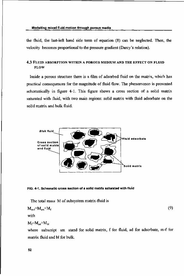
Modelling mixed fluid motion through porous media
the fluid, the last-left hand side term of equation (8) can be neglected. Then, the
velocity becomes proportional to the pressure gradient (Darcy's relation).
4.3 FLUID ABSORPTION WITHIN A POROUS MEDIUM AND THE EFFECT ON FLUID
FLOW
Inside a porous structure there is a film of adsorbed fluid on the matrix, which has
practical consequences for the magnitude of fluid flow. The phenomenon is presented
schematically in figure 4-1. This figure shows a cross section of a solid matrix
saturated with fluid, with two main regions: solid matrix with fluid adsorbate on the
solid matrix and bulk fluid.
Bluk fluid
Cross section of solid matrix and fluid
Fluid adsorbate
Solid matrix
FIG. 4-1. Schematic cross section of a solid matrix saturated with fluid
The total mass M of subsystem matrix-fluid is
Mm.,=Msm+Mf (9)
with
Mf=Mad+Mbl
where subscript sm stand for solid matrix, f for fluid, ad for adsorbate, m-f for
matrix fluid and bl for bulk.
52
Chapter 4
The change of fluid adsorbate and bulk fluid within the medium influences the
amount of fluid flow through the medium. Those interactions can be described using
thermodynamics concepts. In particular, the first law of thermodynamics is used. This
law is a statement of the principle of conservation of energy, and relates the change of
internal energy of a system with thermal, mechanical and diffusive interactions
between the system and the surroundings.
4.3.1 Mass change in the subsystem matrix-fluid
Following the formalism developed by Heitor [5], and assuming that the superficial
stress of fluid within the matrix and in the surroundings is equal, the equation (A-5)
presented in the Appendix become
T(ÔSt)=ÔF.Ôrm.rÔP SV„,f+Sä) SMm.f+ÔT ÔSm.f (10)
with
ÔF=Si(ÔFi)
and
T(8St)>0
where V represents the volume, M the mass, co the chemical potential, SS t the creation
of entropy in the process, S the entropy, r the vector position and F the vector force
(EjFj the total of F due to the effects of mechanical means, gravity, wind, etc.).
The mass change in the subsystem matrix-fluid is given by
ÔMsm+ÔMad+ÔMbl =8Mm.r çv (ÔP+ôp)+çsÔT+T(SSt/ôco) (11)
with
Çv= (oVm./ôco)
çs=-(ÔSmy5a))
ôp=(I.ÔF)/ÔAm.f
where the coefficient çv define the rate between the variation of volume of subsystem
53
Modelling mixed fluid motion through porous media
composed by the solid matrix saturated with fluid and the variation in chemical
potential of the whole system, the coefficient çs defines the rate between the variation
of entropy of subsystem matrix-fluid and the variation in chemical potential of the
whole system, and I represents the unit vector.
Equation (11) relates the change of mass in a subsystem matrix-fluid with intensive
quantities (P,p,T) and generalises the relation obtained by Heitor et al. [6]. This
equation is useful for the study of porous media. Especially on the optimisation of
strategies related to the injection, maintenance and extraction of fluid in porous media,
as well as to provide additional information to be used in the motion equation.
Near the equilibrium, the last right-hand side term of equation (11) is small enough
to approximate the equation by
SMm.f=çv(SP+Sp)+çsST (12)
For isobaric conditions
ÔMm.f=çsÔT (13.1)
and for isothermal conditions
ÔMm.f=çv(ÔP+ôp) (13.2)
Although the parameters çv and çs are physically defined here, theoretical values are
rather difficult to find. Consequently, those parameters should be evaluated based on
experiments [6].
4.3.2 Effects on fluid flow
As the mass of solid matrix is constant and the variation of 8Mm_f, 8p, 5F and 8T are
in spatial coordinates (8x,8y,8z), equation (12) yields
VMm.r çv (VP+Vp)+çsVT (14)
So
VP=-Vp+(Vm.t/çv)Vp-(çs/çv)VT (15)
From the analysis of equation (15), it can be concluded that in absence of density
54
Chapter 4
and temperature gradients VP=-Vp. That is, the pressure gradient (Vp) due to the
action of external force is independent of parameters çv and qs. If Vp=0
VP=(Vm. f/çv)Vp-(çs/çv)VT (16)
that is, the pressure gradient (VP) depends on çv and çs. The following situations can
occur:
• ç s=0: VP is only due to gradient of p,
• qv»0 ar*d Çs«0; VP is only due to gradient of the temperature,
• çv>0 and çs<0: VP can occur due to gradient of concentration and the gradient
of the temperature.
These results are in agreement with the work ofHeitor et al. [6].
Insertion of equation (16) into the momentum equation gives new insight of the
driving potential on the fluid flow. Substitution of equation (16) in (4) yields
(pf/e) Ôu/ôt+(pf /62)(u.V)u=-[-(Vm.f/çv)V p+ (ÇS/ÇV)VT]-K-'U
-Pf<T|u|u+(pf/8) V2u (17;
Equation (17) shows how the gradients of p and T are related to the fluid velocity.
The interaction between fluid and matrix defined by parameters çs and çv is also
clearly included.
4.4 METHODOLOGIES FOR MEASURING PARAMETERS ÇV> ÇS> K? °~>£ A N D Ä-EFF
In order to use the previous mass, momentum and energy conservation equations,
the parameters çv, Çs> K> ®> -̂eff a r ,d £ must be known. These are obtained by fitting
experimental data with appropriate equations (equations (1), (5.1), (7) and (13)). Then,
the following set of experiments must be performed
• the parameters K and a can be obtained from forcing the air through the
porous medium producing a constant pressure drop over the sample (DC-
pressurisation method) and fitting experimental data with the help of
55
Modelling mixed fluid motion through porous media
equation (7) [8]. This method of measuring is the subject of the study
performed by Miguel et al. [9] using porous screens,
• measuring the fluid volume within porous media and the volume of solid
matrix with fluid, the porosity s is obtained from the ratio between them
(equation (1)),
• Xeff can be measured, for example, with the nonsteady state probe method
based on the measurement of the temperature response [10] or with a steady
state method based on the well known Fourier law of heat conduction,
• parameters çv and çs can be obtained from isothermal and isobaric
conditions and fitting experimental data with equations (13.1) and
(13.2). This will be the subject of the next section.
4.5 EXPERIMENTAL DETERMINATION OF PARAMETERS ÇV AND ÇS FOR DIFFERENT
POROUS MEDIA
In order to evaluate parameters çv and çs, a set of experiments was performed using
different porous media. The media used were samples of a sponge
(p=3.23xl0"2 g/cm3), a brick (p=1.92 g/cm3), and two thin greenhouse porous screens
trade mark "ECONET SF" (p=0.352 g/cm3) and "PH 20" (p=0.304 g/cm3).
First, to have the samples understudy matrix free from fluid, they were placed in an
evacuated oven at a temperature of 102°C during six days. Then, the samples were
placed in an exsiccator and exposed to air with various constant water vapour
pressures and at various constant temperatures during fifteen to twenty five days, to
obtain an equilibrium between the atmosphere of the exsiccator and the samples. The
samples were exposed to temperature levels between 10 °C and 30 °C and water
vapour pressures between 201 Pa and 1760 Pa. The various water vapour pressures
were achieved using several saturated solutions (NaOH, LiCl, CaCl2, etc.). The
variation of saturated water vapour pressure with temperature was taken into account.
The possible effect of hysteresis on the measurements was studied by performing
56
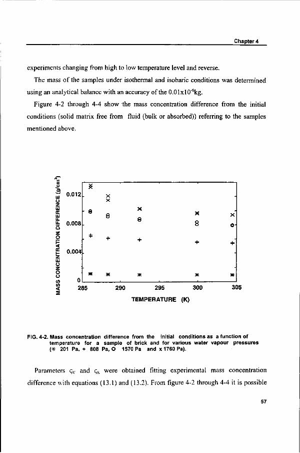
Chapter 4
experiments changing from high to low temperature level and reverse.
The mass of the samples under isothermal and isobaric conditions was determined
using an analytical balance with an accuracy of the 0.01xl0"6kg.
Figure 4-2 through 4-4 show the mass concentration difference from the initial
conditions (solid matrix free from fluid (bulk or absorbed)) referring to the samples
mentioned above.
S 0012 Ü z uj cc UJ
t 0.008 o z o
JE 0.004 UI ü z O o W
< S
a -
- ©
*
m
X X
8
+
X
8
+
*
8
+
m
•
X
o-
+
K
285 290 295 300
TEMPERATURE (K)
305
FIG. 4-2. Mass concentration difference from the initial conditions as a function of temperature for a sample of brick and for various water vapour pressures ( * 201 Pa, + 808 Pa, O 1570 Pa and x 1760 Pa).
Parameters çv and çs were obtained fitting experimental mass concentration
difference with equations (13.1) and (13.2). From figure 4-2 through 4-4 it is possible
57
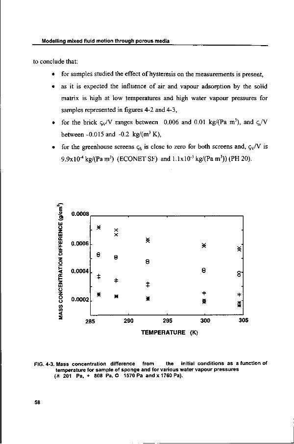
Modelling mixed fluid motion through porous media
to conclude that:
• for samples studied the effect of hysteresis on the measurements is present,
• as it is expected the influence of air and vapour adsorption by the solid
matrix is high at low temperatures and high water vapour pressures for
samples represented in figures 4-2 and 4-3,
• for the brick qw/V ranges between 0.006 and 0.01 kg/(Pa m3), and çs/V
between-0.015 and -0.2 kg/(m3 K),
• for the greenhouse screens çs is close to zero for both screens and, çv/V is
9.9X10⁻⁴ kg/(Pa m3) (ECONET SF) and l.lxlO"3 kg/(Pa m3)) (PH 20).
* 0.0008
m o z UJ
oc UJ 0.0006 u. O z o < 0.0004 er H Z UJ ü z O Ü (/) tn <
0.0002
. *
s
" *
*
X X
8
*
m
i
8
*
*
X
8
4=
tu
-
X •
8-
4=
i'
285 290 295 300
TEMPERATURE (K)
305
FIG. 4-3. Mass concentration difference from the initial conditions as a function of temperature for sample of sponge and for various water vapour pressures ( * 201 Pa, + 808 Pa, O 1570 Pa and x 1760 Pa).
58
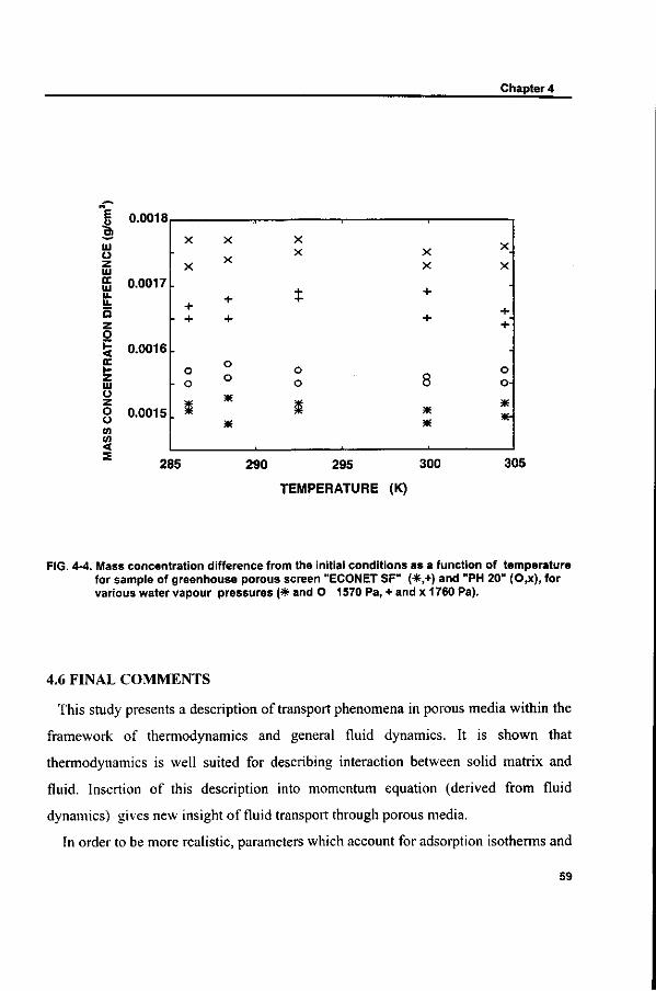
Chapter 4
E
UJ o z 111 DC UJ
a z o
tr i -z UJ ü z o Ü en en <
0.0017
0.0016
0.0015
X
X
+ - +
•
o - o
. *
X
X
+
+
o o *
*
X X
t
o o
• " - • ' • • l
X X
+
+
8
*
X
+ +"
-
o o-
*
285 290 295 300
TEMPERATURE (K)
305
FIG. 4-4. Mass concentration difference from the initial conditions as a function of temperature for sample of greenhouse porous screen "ECONET SF" (*,+) and "PH 20" (O.x), for various water vapour pressures ( * and O 1570 Pa, + and x 1760 Pa).
4.6 FINAL COMMENTS
This study presents a description of transport phenomena in porous media within the
framework of thermodynamics and general fluid dynamics. It is shown that
thermodynamics is well suited for describing interaction between solid matrix and
fluid. Insertion of this description into momentum equation (derived from fluid
dynamics) gives new insight of fluid transport through porous media.
In order to be more realistic, parameters which account for adsoiption isotherms and
59
Modelling mixed fluid motion through porous media
adsorption isobars were determinated based on experiments for different porous
media. Based upon the results obtained it is clear that adsorption isobars and
isotherms (çv and çs) has significant importance on sponge and brick samples. For
greenhouse porous screens çs was close to zero , that is, the temperature doesn't have
significant effect on air absorption by the solid matrix.
4.7 REFERENCES
[1] Combarnous, M. and Bernard, D. 1988. Modelling free convection in porous
media: from academic cases to real configurations. Proceedings of the 1988 National
Heat Transfer Conference, Houston, USA
[2] Bear, J. 1972. Dynamics of fluids in porous media, American Elsevier
Environmental Sciences Series, New York, USA
[3] Miguel, A. F., van de Braak, N. J., Silva, A. M. and Bot, G. P. A. 1998.
Forced fluid motion through permeable materials, Building and Environment (in
press)
[4] Brinkman, M.C. 1947. A calculation of the viscous force exerted by a flowing
fluid on a dense swarm of the particles, Appl. Sei. Res., Al , 27-34
[5] Heitor, A. 1992. Formalismo termodinâmico com base nos parâmetros criticos
com aplicaçôes ao estudo das capacidades térmicas e dos processus reversiveis. Ph.D.
Dissertation, University of Évora, Portugal [in Portuguese]
[6] Heitor, A., Silva, O. and Rosa, R. 1994. Heat and mass transfer in porous
materials, Characterization of Porous Solids III, 87, 207-209
[7] Chapman, S. and Cowling, T. C. 1970. The mathematical theory of non-uniform
gases. Cambridge University Press, Cambridge, United Kingdom
[8] Forchheimer, P. 1901. Wasserbewegung durch boden, Z. Ver. Deustsch., 45,
1782-1788 [in German]
[9] Miguel, A. F., van de Braak, N. J., Silva, A. M. and Bot, G. P. A. 1997.
Analysis of the airflow characteristics of greenhouse screening materials, J. Agric.
60
Chapter 4
Engng. Research 67, 105-112.
[10] Loon, W. K. P. van 1991. Heat and mass transfer in frozen porous media. Ph.D.
Dissertation, Agricultural Wageningen University. The Netherlands
4.8 APPENDIX
Thermodynamics analysis: budget equation of properties of a system
The following formulation is based on a formalism presented by Heitor (1993) for
the interaction between two thermodynamic subsystems.
Consider a thermodynamic system consisting of n subsystems. The principle of
conservation requires that, for each subsystem, the change in internal energy is a
consequence of thermal, mechanical and diffusive interactions between the subsystem
and its surroundings. This constitutes the first law of thermodynamic and from a
mathematical point of view we can write for the total system
5U=Zn(ÔUn)=Sn(FnÔrn+CnSAn-Pn5Vn+TnÔSn+conSMn) (A-l)
where Un is the internal energy, Tn the temperature, Pn the pressure, Vn the volume, Mn
the mass, con the chemical potential, Sn the entropy, and Çn, Fn and rn are the vectors
for superficial stress, force and position of the subsystem n, respectively.
The subsystems can exchange quantities like energy, entropy, volume and mass. The
budget equation for a quantity A is then
In(5An)=ÔAt (A-2)
where 8An is the variation of the quantity A in the subsystem n and 8At represent the
creation or destruction of quantity A in the transfer process.
For the case of conservatives quantities like energy, volume and mass we only have
to write
Sn(ÔAn)=0 (A-3.1)
but for the entropy the second law of thermodynamics imposes
61
Modelling mixed fluid motion through porous media
Zn(ÔSn)=ÔSt (A-3.2)
where Sn is the entropy in subsystem n.
Specifically the exchange of A between a subsystem s and the remaining
thermodynamic system (n^s) can be written as
ÔAt=2n,s(ÔAn-ÔAs) (A-4)
Taking into account equations (A-l) through (A-4) we can write
Ts5St=2n,s(Fn-Fs)5rn+En,s(Çn-Çs)ÔAn-Zn,s(P„-Ps)5Vn+Zn,s(Tn-Ts)ÔS11+
En,s(cûn-cos)SMn>0 (A-5)
were Ts8St is the so-called availability function.
Equation (A-5) describes the thermal, mechanical and diffusive interactions between
the subsystem s and the remains thermodynamic system composed by the
subsystems n*s.
4.9 NOMENCLATURE
A
c
C
F
M
P,P
S
T
U
u
V
Greek
S
A
62
area [m ]
coefficient related with porous inertia
specific heat [J kg'K"1]
force [N]
mass [kg]
pressure [Pa]
entropy [J K"1]
temperature [K]
internal energy [J]
velocity [m s"1]
volume [m3].
symbols
porosity
quantity like volume, entropy or mass
Chapter 4
n p
a
K
X
CD
Subscripts
ad
bl
eff
f
m-f
sm
dynamic viscosity [Pa s]
density [kg m"3]
inertial coefficient [m1]
fluid conductivity [m3s kg"1]
thermal conductivity [W m^K."1]
chemical potential [J kg"1].
adsorbate
bulk
effective
fluid
solid matrix - fluid
solid.
63
64
5. Analysis of the airflow characteristics of greenhouse
screening materials +
Abstract: Experiments and analyses were conducted to examine the airflow
characteristics of some currently employed greenhouse screens and the ability to
predict airflow through them. Nine different thermal, shading and insect screens were
tested and their airflow characteristics were defined, based on the Forchheimer
equation, in terms of permeability and porosity. Further, an analysis was made of the
effect on these characteristics of damage caused by handling of the screen materials.
Experiments demonstrated that thermal screens have permeabilities of close to
10"nm2 and some thermal screens, mainly woven sheet screens, can be damaged by
handling, whereby the permeability is increased up to 3.5 times.
5.1 INTRODUCTION
The potential benefits resulting from the use of screens in protected horticulture have
been increasingly recognised in recent years. Screens are a simple and successful
means for avoiding night-time heat loss and controlling the solar radiation inside a
greenhouse, as well as for preventing the entrance of birds and insects. In order to
optimise the use of screens in agriculture, an extensive knowledge of their
characteristics is required. A number of authors have worked on the measurement of
the optical or radiometric characteristics of different materials used for screens [1,2],
while others have worked on the measurement of the airflow characteristics
(characteristics related to fluid transport through a screen). These characteristics have
been evaluated in empirical terms of "permeability" based on the Darcy's law [3,4], or
"coefficient of discharge" based on Bernoulli's flow theory [5,6].
The purpose of the present study is to discuss the more general physics of transport
phenomena through permeable materials in order to provide a simple and accurate
+ J. Ag. Engng. Research 67,105-112
Airflow characteristics of greenhouse screening materials
methodology for identifying the airflow characteristics of materials currently used as
screens. Through experiments conducted in two different experimental arrangements
these characteristics were determined in the range of Reynolds number commonly
observed for porous thermal screens and porous insect screens. An analysis is also
included of the effect of overall damage caused by opening and closing the screen.
5.2 PRESSURE DROP AND FLOW RELATIONSHIP
For one-dimensional mass transfer through a permeable material the motion
equation can be expressed as [7]
(p/e)du/a+(p/e2)u(5u/ôx)=-dp/Sx-(u/K)u-p(Y/K1/2) |u|u+(p/8)(52u/5x2) (1)
with
U = 8 U j
where u is the superficial fluid velocity, us the velocity through the material, p the
density, p the pressure, u, the dynamic viscosity, Y the inertia factor and x the direction
of flow. The parameter E is the porosity and represents the volume fraction of fluid
contained within the total volume of the medium, while parameter K is the
permeability of the medium and represents the ability of the medium to transmit the
fluid through it.
The dimensionless factor Y is often obtained from Ergun [8] using the relationship
obtained in packed columns of spheres
Y=l.75/(150s3)172 (=0.143/8'5) (2)
5.3 MOTION EQUATION AND AIR FLOW CHARACTERISTICS OF A POROUS SCREEN
To illustrate the magnitude of the permeability of a permeable material and
subsequently evaluate its effects on the airflow, consider the definition of
permeability presented by Lebon and Cloot [9] based on kinetic gas theory. According
to this theory, the permeability is related to the reciprocal of the collision frequency of
66
Chapter 5
diffusing particles and the kinematic fluid viscosity. For a porous material the collision
frequency is greater than 103 Hz [10] and as the kinematic fluid viscosity of air is the
order of magnitude of 10"5 m V , the permeability will be of a magnitude less than
10"7 m2 (the second and third right-hand side terms of Eqn (1) are of great importance).
For openings (windows, doors) the collision frequency will be close to zero and
consequently the permeability K-»oc. That means, the second and third right-hand side
terms of Eqn (1) become zero and for openings we obtain the standard Navier-Stokes
equation. For a steady, non-viscous flow, the Navier-Stokes equation can be integrated
along a streamline and we obtain the Bernoulli equation.
Consider forced flow through a porous material (the study of openings is beyond the
scope of this paper). According to Bear and Bachmat [11], for Reynolds numbers
(Re) smaller than 150 the flow is incompressible (9u/9x=0). Then the second left-
hand side term and the fourth right-hand side term of Eqn (1) can be discarded. For a
steady flow, Eqn (1) becomes
(|i/K)u+p(Y/Kl/2) |u|u=dp/Sx (3)
Eqn (3) is the well known Forchheimer equation for highly porous materials. For
very small velocities [11] (Re<l) the quadratic term in velocity can be neglected and
we obtain the Darcy law.
u=(K/fi)dp/ôx (4)
Darcy's law is the equation which defines permeability of a porous material.
Instead of permeability some authors [5,6] use the discharge coefficient, resorting to
Bernoulli's equation, to characterise a screen. According to the above we can therefore
conclude that the discharge coefficient will be appropriate only when convective
inertia effects are present (Re>150). Under commonly observed situations this will be
very unlikely for porous screens. Notice that, for wind velocities of 5 m/s (wind
pressure approximately 15 Pa) the Reynolds number (Re=pUjd/u) for a typical thermal
screen is 5 (mesh size d=0.03 mm) and for an insect screen is 89 (mesh size
d=0.11 mm).
67
Airflow characteristics of greenhouse screening materials
As the subject of this study is porous screens, these will be characterised in terms of
permeability and porosity, using Eqns (3) and (4).
5.4 EXPERIMENTAL STUDY
In order to obtain the airflow characteristics of porous screens as well as the inertial
factor Y (Eqns (1) and (2)), experiments were carried out using two different test
arrangements. Although both apparatus have the same principle, in that air is forced
through the test samples in order to create a pressure drop, their ranges of applicability
are different: one is used for Re less than 1 (in accordance with the range of Eqn (4))
and the other for Re greater than 1 and less than 100 (in accordance with the range of
Eqn (3)).
Description of test apparatus
For Re<l, the screen samples (diameter 6 cm) were mounted in a tube (internal
diameter 6 cm and length 20 cm) separated by fibre rings of 0.5 cm thickness
(Fig. 5-la) containing 20 pieces of each screen sample (in order to ensure a larger
pressure drop). The tube was connected to the upper side of a cylindrical reservoir
(radius 15 cm and length 120 cm) connected by a stiff tube (diameter 6 cm)
(Fig. 5-lb). The measurements are based on the pressure drop caused by natural
suction of air through the samples as a result of water flow induced by gravity.
The volumetric flow rate was controlled using a valve in the outlet duct, and was
measured using a glass and a stopwatch. The pressure drop was measured using an
inclined tube manometer Lambrecht KG type 655 (accuracy 1 mm of alcohol), with
one part connected to the test apparatus and the other connected to the air in the
experimental room.
For l<Re<100, the experiments were carried out in a test apparatus as shown in
Fig. 5-2a. It comprises a test box (2.5 m x 2.5 m x 2.5 m) with two screens (installed
at 1.60 m from the inlet side and separated by 10 cm) in order to ensure that a uniform
68
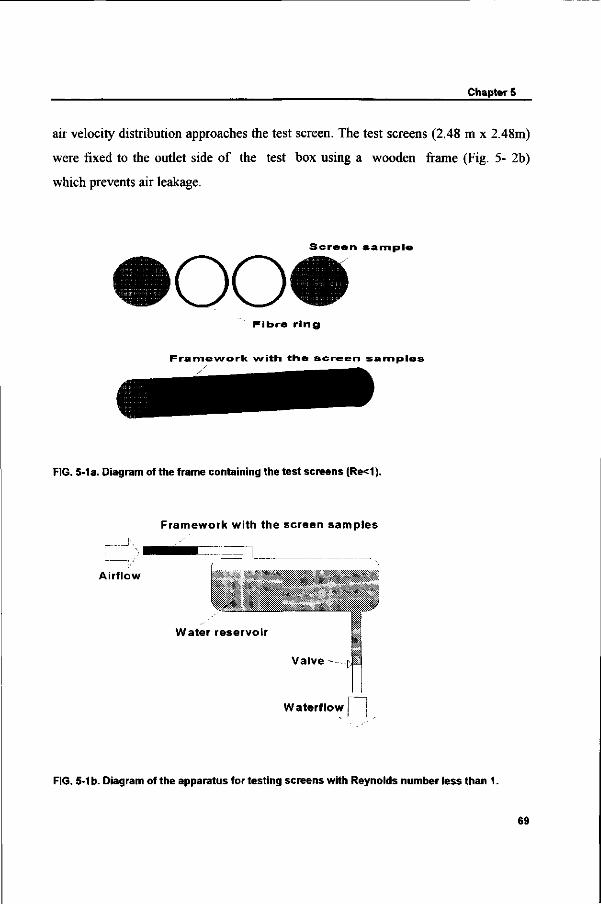
Chapter 5
air velocity distribution approaches the test screen. The test screens (2.48 m x 2.48m)
were fixed to the outlet side of the test box using a wooden frame (Fig. 5- 2b)
which prevents air leakage.
S c r e e n s a m p l e
POO F i b r e r i n g
F r a m e w o r k w i t h t h e s c r e e n s a m p l e s
FIG. 5-1 a. Diagram of the frame containing the test screens (Re<1 ).
Framework with the screen samples
Airflow
V
Water reservoir
Valve
Waterflow
FIG. 5-1 b. Diagram of the apparatus for testing screens with Reynolds number less than 1.
69
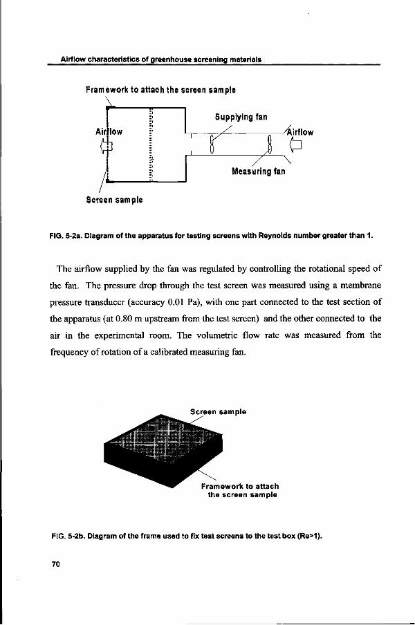
Airflow characteristics of greenhouse screening materials
Framework to attach the screen sample
Supplying fan
/Airflow
0 Measuring fan
Screen sample
FIG. 5-2a. Diagram of the apparatus for testing screens with Reynolds number greater than 1.
The airflow supplied by the fan was regulated by controlling the rotational speed of
the fan. The pressure drop through the test screen was measured using a membrane
pressure transducer (accuracy 0.01 Pa), with one part connected to the test section of
the apparatus (at 0.80 m upstream from the test screen) and the other connected to the
air in the experimental room. The volumetric flow rate was measured from the
frequency of rotation of a calibrated measuring fan.
Screen sample
Framework to attach the screen sample
FIG. 5-2b. Diagram of the frame used to fix test screens to the test box (Re>1).
70
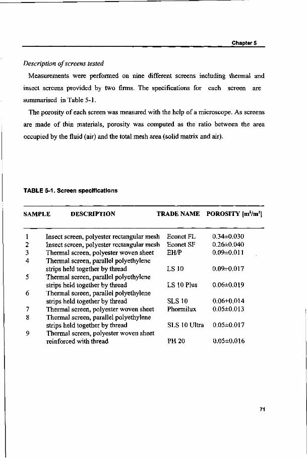
Chapter 5
Description of screens tested
Measurements were performed on nine different screens including thermal and
insect screens provided by two firms. The specifications for each screen are
summarised in Table 5-1.
The porosity of each screen was measured with the help of a microscope. As screens
are made of thin materials, porosity was computed as the ratio between the area
occupied by the fluid (air) and the total mesh area (solid matrix and air).
TABLE 5-1. Screen specifications
SAMPLE DESCRIPTION TRADE NAME POROSITY [m2/m2]
1 Insect screen, polyester rectangular mesh 2 Insect screen, polyester rectangular mesh 3 Thermal screen, polyester woven sheet 4 Thermal screen, parallel polyethylene
strips held together by thread 5 Thermal screen, parallel polyethylene
strips held together by thread 6 Thermal screen, parallel polyethylene
strips held together by thread 7 Thermal screen, polyester woven sheet 8 Thermal screen, parallel polyethylene
strips held together by thread 9 Thermal screen, polyester woven sheet
reinforced with thread
Econet FL Econet SF EH/P
LS 10
LS 10 Plus
SLS10 Phormilux
SLS 10 Ultra
PH20
0.34±0.030 0.26±0.040 0.09±0.011
0.09±0.017
0.06±0.019
0.06±0.014 0.05±0.013
0.05±0.017
0.05±0.016
71
Airflow characteristics of greenhouse screening materials
Description of the experiments
For each screen sample, measurements were taken using the test apparatus shown in
Figs. 5-1 and 5-2 in order to obtain the volumetric flow rate and the pressure drop
through the sample.
Variation in screen porosity and even tearing can occur due to tension created by the
airflow. In order to prevent this, in accordance with the explanation in appendix,
experiments were carried out with pressures lower than 150 Pa.
In order to take asymmetry in the screen structure into account, the tests were carried
out with the air flowing in both directions through the screen. The possible effect of
hysteresis on the measurements was accounted for by performing experiments
between low and high airflow rates, and the reverse.
First, individual new screen samples were tested. As handling (opening/closing)
easily damages some screens, tests were also made on screens which had been folded
ten times.
During the tests, the data were collected every 15 s for periods of 10-20 min to be
sure that conditions were at steady state.
5.5 RESULTS AND DISCUSSION
For each material tested, the data resulting from the experiments performed were
plotted as pressure drop versus the superficial velocity, as shown in Figs. 5-3 to 5-5.
In all the samples tested, the equation that best seemed to fit the curves obtained was a
second order polynomial Ap=au2+bu+c (i.e. the data presented fit Eqn (3) the
Forchheimer equation). The coefficients are presented in Table 5-2.
Therefore, provided the best fit coefficients are found (zero order term can be
neglected compared with the other terms), the permeability and factor Y can be
calculated from Eqn (3) (fluid properties included in Eqn (3) were obtained for the
mean air temperature of experimental room). The results are listed in Table 5-3.
72
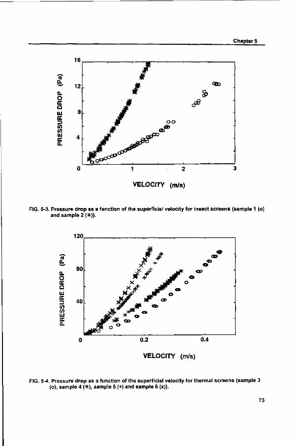
Chapter 5
co O .
a. O Œ Q UJ £E D (/) V) UJ CC
a.
1 2
VELOCITY (m/s)
FIG. 5-3. Pressure drop as a function of the superficial velocity for insect screens (sample 1 (o) and sample 2 (*)).
to a.
120
Q. O Œ
a Ui ΠZ> C/> CO UJ cc a.
8 0 .
40
$ J-
/ / X »jj
'*̂ " .fll* w^*^*» J T . JP «*>
* j iF 5W «a> ijPjj (Q*
*rf*^ °.
J F o
f € »
O
9
o>
0.2 0.4
VELOCITY (m/s)
FIG. 5-4. Pressure drop as a function of the superficial velocity for thermal screens (sample 3 (o), sample 4 (•*), sample 5 (+) and sample 6 (x)).
73
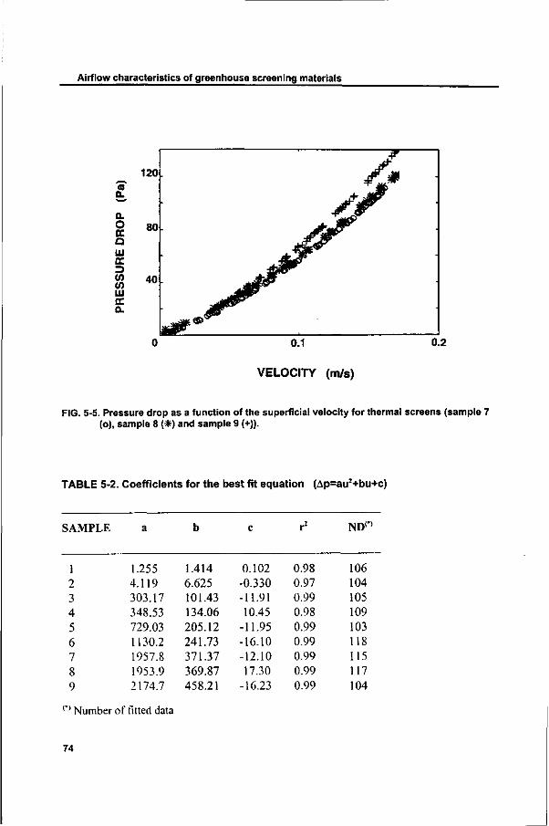
Airflow characteristics of greenhouse screening materials
120. «J
a. a. O cc o Ui CC
(/) (O Ol OC
o.
0.1
VELOCITY (m/s)
FIG. 5-5. Pressure drop as a function of the superficial velocity for thermal screens (sample 7 (o), sample 8 (*) and sample 9 (+)).
TABLE 5-2.
SAMPLE
1 2 3 4 5 6 7 8 9
Coefficients for the best fit equal
a
1.255 4.119 303.17 348.53 729.03 1130.2 1957.8 1953.9 2174.7
b
1.414 6.625 101.43 134.06 205.12 241.73 371.37 369.87 458.21
c
0.102 -0.330 -11.91 10.45
-11.95 -16.10 -12.10 17.30
-16.23
ion (Ap=
r2
0.98 0.97 0.99 0.98 0.99 0.99 0.99 0.99 0.99
:au2+bu+c)
NDn
106 104 105 109 103 118 115 117 104
1 Number of fitted data
74
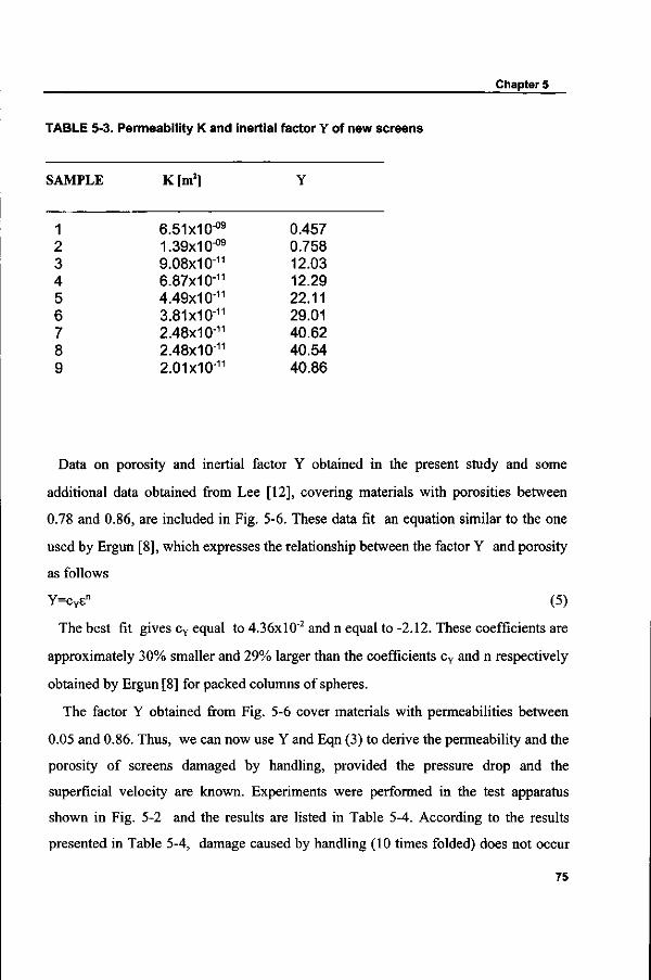
Chapter 5
TABLE 5-3. Permeability K and inertial factor Y of new screens
SAMPLE
1 2 3 4 5 6 7 8 9
K[m2]
6.51 x1009
1.39x1009
9.08x10"11
6.87x10"11
4.49x10" 3.81x10"11
2.48x10"11
2.48x10"11
2.01x10'11
Y
0.457 0.758 12.03 12.29 22.11 29.01 40.62 40.54 40.86
Data on porosity and inertial factor Y obtained in the present study and some
additional data obtained from Lee [12], covering materials with porosities between
0.78 and 0.86, are included in Fig. 5-6. These data fit an equation similar to the one
used by Ergun [8], which expresses the relationship between the factor Y and porosity
as follows
Y=cYen (5)
The best fit gives cY equal to 4.36xl0"2 and n equal to-2.12. These coefficients are
approximately 30% smaller and 29% larger than the coefficients cY and n respectively
obtained by Ergun [8] for packed columns of spheres.
The factor Y obtained from Fig. 5-6 cover materials with permeabilities between
0.05 and 0.86. Thus, we can now use Y and Eqn (3) to derive the permeability and the
porosity of screens damaged by handling, provided the pressure drop and the
superficial velocity are known. Experiments were performed in the test apparatus
shown in Fig. 5-2 and the results are listed in Table 5-4. According to the results
presented in Table 5-4, damage caused by handling (10 times folded) does not occur
75
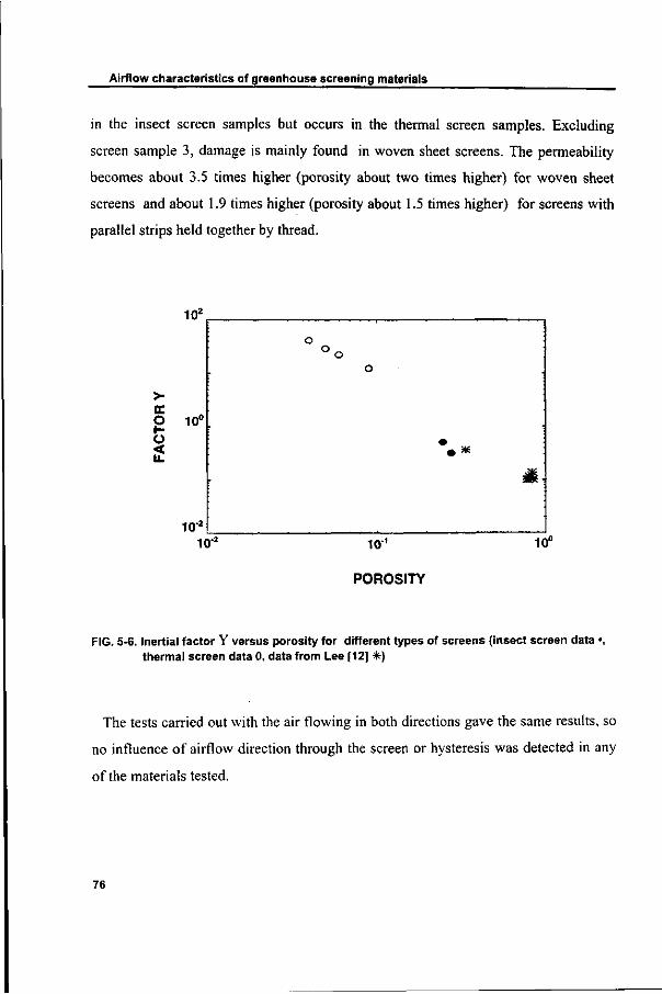
Airflow characteristics of greenhouse screening materials
in the insect screen samples but occurs in the thermal screen samples. Excluding
screen sample 3, damage is mainly found in woven sheet screens. The permeability
becomes about 3.5 times higher (porosity about two times higher) for woven sheet
screens and about 1.9 times higher (porosity about 1.5 times higher) for screens with
parallel strips held together by thread.
FIG. 5-6. Inertial factor Y versus porosity for different types of screens (insect screen data •, thermal screen data 0, data from Lee [12] •*•)
The tests carried out with the air flowing in both directions gave the same results, so
no influence of airflow direction through the screen or hysteresis was detected in any
of the materials tested.
76
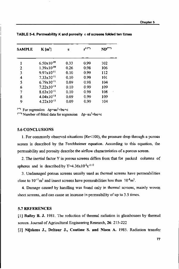
Chapter 5
TABLE 5-4. Permeability K and porosity 8 of screens folded ten times
SAMPLE
1 2 3 4 5 6 7 8 9
K[m2]
6.50X10"09
1.39xl009
9.97x10"" 7.33x10-" 6.79x10-" 7.22x10"" 8.63x10" 4.04x10" 4.22x10""
s
0.33 0.26 0.10 0.10 0.09 0.10 0.10 0.09 0.09
rM**)
0.99 0.98 0.99 0.99 0.98 0.99 0.99 0.99 0.99
ND<"*>
102 106 112 101 104 109 108 109 104
<**) For regression Ap=au2+bu+c <***) Number of fitted data for regression Ap=au2+bu+c
5.6 CONCLUSIONS
1. For commonly observed situations (Re<100), the pressure drop through a porous
screen is described by the Forchheimer equation. According to this equation, the
permeability and porosity describe the airflow characteristics of a porous screen.
2. The inertial factor Y in porous screens differs from that for packed columns of
spheres and is described by Y=4.36xl0~2e-2'2
3. Undamaged porous screens usually used as thermal screens have permeabilities
close to 10"m2 and insect screens have permeabilities less than 10"8m2.
4. Damage caused by handling was found only in thermal screens, mainly woven
sheet screens, and can cause an increase in permeability of up to 3.5 times.
5.7 REFERENCES
[1] Bailey B. J. 1981. The reduction of thermal radiation in glasshouses by thermal
screen. Journal of Agricultural Engineering Research, 26: 215-222
[2] Nijskens J., Deltour J., Coutisse S. and Nisen A. 1985. Radiation transfer
77
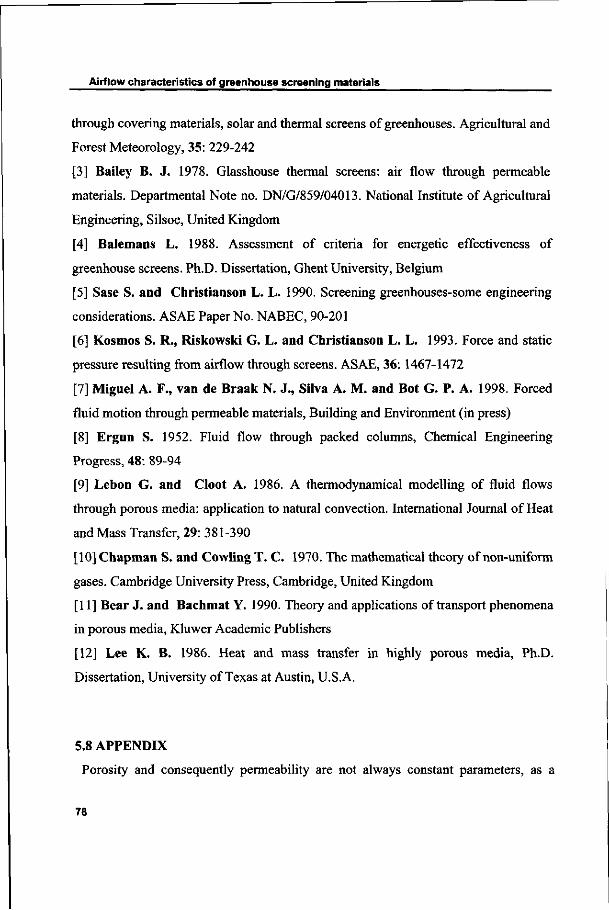
Airflow characteristics of greenhouse screening materials
through covering materials, solar and thermal screens of greenhouses. Agricultural and
Forest Meteorology, 35: 229-242
[3] Bailey B. J. 1978. Glasshouse thermal screens: air flow through permeable
materials. Departmental Note no. DN/G/859/04013. National Institute of Agricultural
Engineering, Silsoe, United Kingdom
[4] Balemans L. 1988. Assessment of criteria for energetic effectiveness of
greenhouse screens. Ph.D. Dissertation, Ghent University, Belgium
[5] Sase S. and Christianson L. L. 1990. Screening greenhouses-some engineering
considerations. ASAE Paper No. NABEC, 90-201
[6] Kosmos S. R., Riskowski G. L. and Christianson L. L. 1993. Force and static
pressure resulting from airflow through screens. ASAE, 36: 1467-1472
[7] Miguel A. F., van de Braak N. J., Silva A. M. and Bot G. P. A. 1998. Forced
fluid motion through permeable materials, Building and Environment (in press)
[8] Ergun S. 1952. Fluid flow through packed columns, Chemical Engineering
Progress, 48: 89-94
[9] Lebon G. and Cloot A. 1986. A thermodynamical modelling of fluid flows
through porous media: application to natural convection. International Journal of Heat
and Mass Transfer, 29: 381-390
[10] Chapman S. and Cowling T. C. 1970. The mathematical theory of non-uniform
gases. Cambridge University Press, Cambridge, United Kingdom
[11] Bear J. and Bachmat Y. 1990. Theory and applications of transport phenomena
in porous media, Kluwer Academic Publishers
[12] Lee K. B. 1986. Heat and mass transfer in highly porous media, Ph.D.
Dissertation, University of Texas at Austin, U.S.A.
5.8 APPENDIX
Porosity and consequently permeability are not always constant parameters, as a
78
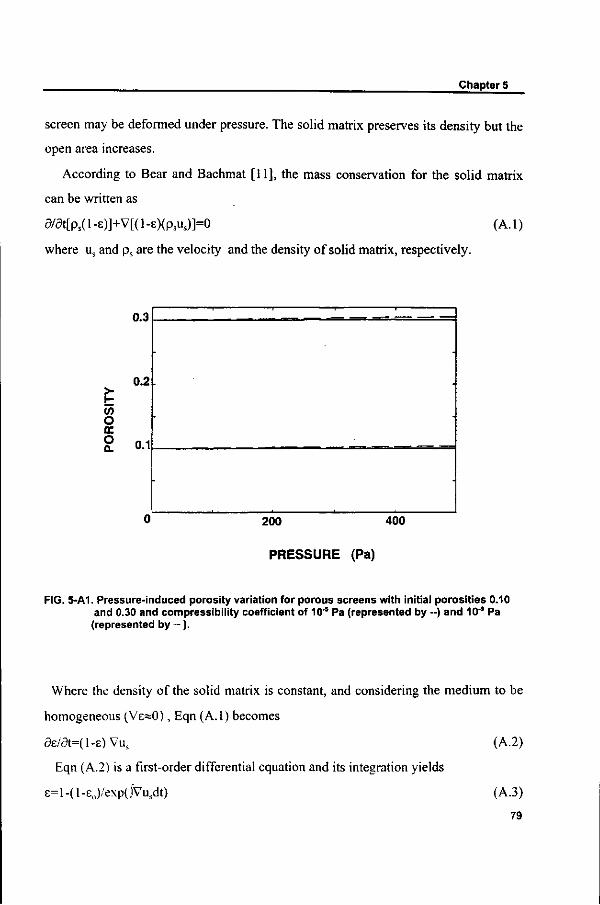
Chapter 5
screen may be deformed under pressure. The solid matrix preserves its density but the
open area increases.
According to Bear and Bachmat [11], the mass conservation for the solid matrix
can be written as
ö/öt[ps( 1 -£)]+V[( 1 -s)(psus)]=0 (A. 1 )
where us and ps are the velocity and the density of solid matrix, respectively.
200 400
PRESSURE (Pa)
FIG. 5-A1. Pressure-induced porosity variation for porous screens with initial porosities 0.10 and 0.30 and compressibility coefficient of 10"5 Pa (represented by --) and 10"9 Pa (represented by — ).
Where the density of the solid matrix is constant, and considering the medium to be
homogeneous (Vs*0), Eqn (A.l) becomes
Se/öt=(l-E)Vus (A.2)
Eqn (A.2) is a first-order differential equation and its integration yields
e=l-(l-e0)/exp(jVusdt) (A.3)
79
Airflow characteristics of greenhouse screening materials
with
jVusdt=u
where e0 is the initial porosity (measured at standard atmospheric pressure) and u the
volumetric strain [11].
For an elastic matrix, the volumetric strain is proportional to the pressure, and Eqn
(A.3) becomes
6=l-(l-80)/exp(T1-1Ap) (A.4)
where r| is the compressibility coefficient of the matrix.
Eqns (A.3) and (A.4) show how the porosity changes with the increase of pressure.
In order to prevent variation in screen porosity during the experiments, a simulation
study is performed based on equation (A.4). Fig. 5-A.l shows the porosity variation
due to pressure for the test screens used (initial porosity 0.10 and 0.30 and
compressibility coefficient of the matrix 10"5 Pa and 10"9 Pa). According to Fig. 5-A.l,
for a pressure drop of less than 150 Pa, the porosity variation from initial conditions
(zero pressure drop) is always less than 0.05%. This pressure is the maximum value
used in the experiments.
5.9 NOMENCLATURE
d mesh size [m]
i j , l unit vectors in direction x, y and z
K permeability of the screen [m2]
p pressure [Pa]
u superficial fluid velocity [ms1]
Uj fluid velocity through a permeable material [ms 1 ]
us velocity of solid matrix [ms1]
Re Reynolds number (Re= p Ujd/ p.)
t time [s]
80
Chapter 5
Y
8
P-
P
V
inertial factor
porosity
dynamic viscosity [Pa s]
density [kg m"3]
(i d/dx+j ô/ôy+1 d/dz)
Subscripts
0
s
initial
solid
81

82
6. PHYSICAL MODELLING OF NATURAL VENTILATION
THROUGH SCREENS AND WINDOWS IN GREENHOUSES +
Abstract: In the previous chapters the physical basis of air exchange through porous
materials and openings were presented. In this chapter, formulation presented in
chapters 2, 3 and 5 is applied to study natural ventilation through screens and window
openings in greenhouses. The wind velocities and air temperature differences which
drive the airflow were characterised. Fluctuations in wind velocity were related to the
mean wind velocity through a parameter which is evaluated based on a power
spectrum analysis. In turn, wind pressure was related to this mean wind velocity such
that turbulence was taken into account. An experimental study was conducted in twin-
span glasshouses in order to validate the approach presented. The predictions made of
airflow versus wind pressure and temperature differences agree reasonably well with
experimental data, differences between them being less than 20%, in general.
6.1 INTRODUCTION
Natural ventilation of a greenhouse is a complex process which depends on the
greenhouse characteristics (number, location and geometry of windows, area of leaks,
etc.) as well as on the external ambient conditions. Although its important impact on
the mass and energy balance which affects the indoor climate conditions, the subject
is far from being fully understood.
As far as is known natural ventilation through greenhouse window openings were
first studied experimentally by Morris and Neale [1] in 1954. Since them much
progress has been made in understanding the phenomena and new challenges appear.
The rather high oil prices reached in the end of the 70's, followed by the wide public
concern about the ecological aspects related to the high quantities of fossil fuel
consumption in the North-western Europe, contributed to the development of new
+ J. Ag. Engng. Research (in press in a modified form)
Physical modelling of natural ventilation in greenhouses
energy saving strategies. The potential energy saving benefits resulting of the use of
screens between the crop and the roof was demonstrated by Bailey [2], Bailey and
Cotton [3] and Silva et al [4], Recently [5], the use of screens in window openings was
adopted in order to prevent the entrance of insects and so decrease the need for use of
chemical pesticides. Consequently, the study of airflow through screens is also an
important topic.
The existing analytical models on the subject can be divided into two categories as
follow:
• Empirical and semi-empirical approaches for the study of airflow through
window openings [6-13] and airflow through screens [2,5,14].
• Governing fluid mechanics equations solved numerically [15-17].
All models in the first category are based on the idea that there is a simple non-linear
relationship between the airflow and the potentials which drive this flow. Such
analyses consider the air inside the greenhouse as incompressible and they are
commonly based on purely empirical correlations or on Bernoulli's equation, resulting
in dimensionless numbers (such as the Euler number) with empirical correction
factors. However, the simplifying assumptions used together with the correction
factors, which are obtained for specific experimental conditions, considerably restrict
the range of validity of this approach.
In the second category of models, a numerical simulation procedure is applied to
solve the continuity equation, the momentum equation and the energy equation, to
determine the velocity, temperature and pressure fields and consequently the flow
patterns inside the greenhouse.
The study presented in this paper has two objects in view:
• to improve understanding of the physics of the air exchange process through
porous screens (thermal, shading or insect) and through window openings.
More specifically, to establish the flow network of a greenhouse with a window
opening and a screen partially or totally open, and to describe the characteristics of
84
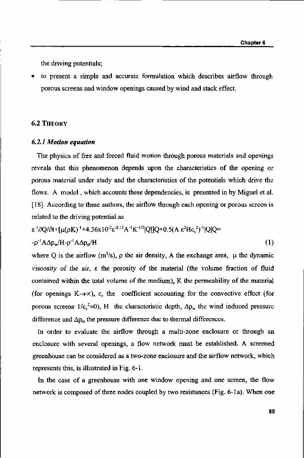
Chapter 6
the driving potentials;
• to present a simple and accurate formulation which describes airflow through
porous screens and window openings caused by wind and stack effect.
6.2 THEORY
6.2.1 Motion equation
The physics of free and forced fluid motion through porous materials and openings
reveals that this phenomenon depends upon the characteristics of the opening or
porous material under study and the characteristics of the potentials which drive the
flows. A model, which accounts these dependencies, is presented in by Miguel et al.
[18]. According to these authors, the airflow through each opening or porous screen is
related to the driving potential as
e-15Q/at+[n(pK)-1+4.36xl0-2E-212A-1K1/2|Q|]Q+0.5(A£2Hcc2)-1|Q|Q=
-p-'AAp^H-p'AAps/H (1)
where Q is the airflow (m3/s), p the air density, A the exchange area, \i the dynamic
viscosity of the air, E the porosity of the material (the volume fraction of fluid
contained within the total volume of the medium), K the permeability of the material
(for openings K-»<x), cc the coefficient accounting for the convective effect (for
porous screens l/cc2«0), H the characteristic depth, Apw the wind induced pressure
difference and Apst the pressure difference due to thermal differences.
In order to evaluate the airflow through a multi-zone enclosure or through an
enclosure with several openings, a flow network must be established. A screened
greenhouse can be considered as a two-zone enclosure and the airflow network, which
represents this, is illustrated in Fig. 6-1.
In the case of a greenhouse with one window opening and one screen, the flow
network is composed of three nodes coupled by two resistances (Fig. 6-la). When one
85
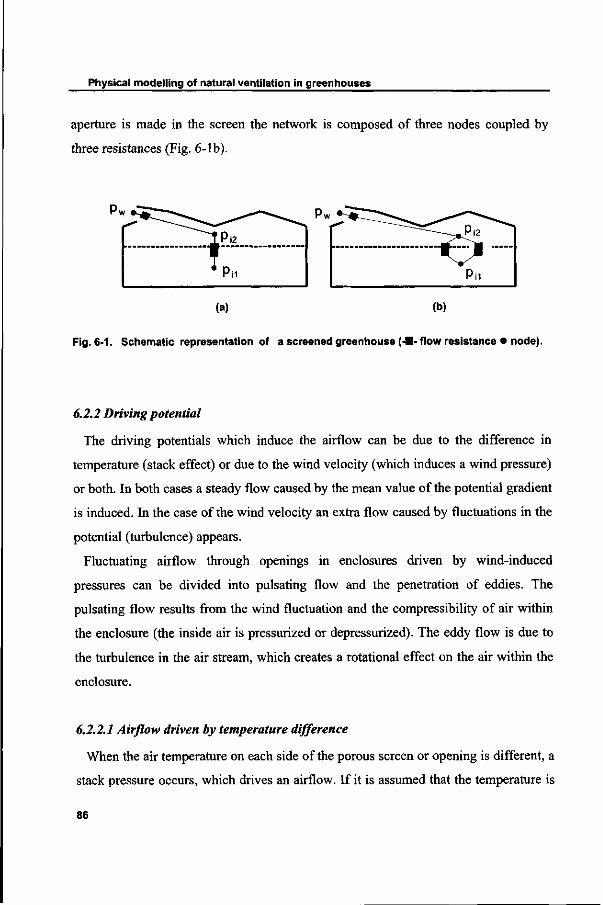
Physical modelling of natural ventilation in greenhouses
aperture is made in the screen the network is composed of three nodes coupled by
three resistances (Fig. 6-lb).
(a) (b)
Fig. 6-1. Schematic representation of a screened greenhouse (-•- flow resistance • node).
6.2.2 Driving potential
The driving potentials which induce the airflow can be due to the difference in
temperature (stack effect) or due to the wind velocity (which induces a wind pressure)
or both. In both cases a steady flow caused by the mean value of the potential gradient
is induced. In the case of the wind velocity an extra flow caused by fluctuations in the
potential (turbulence) appears.
Fluctuating airflow through openings in enclosures driven by wind-induced
pressures can be divided into pulsating flow and the penetration of eddies. The
pulsating flow results from the wind fluctuation and the compressibility of air within
the enclosure (the inside air is pressurized or depressurized). The eddy flow is due to
the turbulence in the air stream, which creates a rotational effect on the air within the
enclosure.
6.2.2.1 Airflow driven by temperature difference
When the air temperature on each side of the porous screen or opening is different, a
stack pressure occurs, which drives an airflow. If it is assumed that the temperature is
86
Chapter 6
different on each side, the pressure difference between the two sides is given by
Apst=Ap g Ah (2)
with
Ap=p ß AT
where AT is the absolute temperature difference measured in the bulk fluid, g the
gravitational acceleration, Ah the vertical height difference through the screen or
opening and ß the coefficient of thermal expansion.
6.2.2.2 Airflow driven by wind velocity (windpressure)
Wind velocity is not a steady quantity when measured over time. The instantaneous
value at time t can be written as the sum of a mean component and a fluctuating
component, that is, ïï and u ' , respectively. The average wind pressure over a time
interval can be related to the wind velocity (in Appendix) by
pw=0.5p(üjt + < u ' w ) (3)
where ïïw is the mean wind velocity and u^ the fluctuations in wind velocity.
Some anemometers give direct readings of the mean velocity and of the root mean
square of the velocity. Assuming u^ to have a Gaussian probability distribution, it is
sometimes convenient to use the following equation instead of (3)
P^O.Spût+pT^uLw (4)
where urn]SW is the root mean square wind velocity.
The more usual situation is to have anemometers which only give readings of mean
velocity. Therefore, an approach which presents wind pressure as a function of mean
velocity only, but does not neglect the effect of the fluctuating component, would be
very useful. For this we need to relate the mean square fluctuating (turbulent)
component of the wind velocity to the mean (static) component of wind velocity.
The dissipation rate of turbulent kinetic energy (r^) can be related directly to the
mean velocity through the inertial subrange spectral density. According to
87
Physical modelling of natural ventilation in greenhouses
Kolmogorov's rule [21]
r,2/3=(3/4)ckr1F(n)(üw/27t)2V/3 (5)
where F(n) is the inertial subrange spectral density, n the frequency and ckl
Kolmogorov's constant (»0.5).
Then, using the relation between the turbulent kinetic energy at a distance z from a
surface and the dissipation rate of turbulent kinetic energy [21],
0.5 <u'w =V5[r ,K(z+z0)]M (6)
the mean square fluctuating component of wind velocity and the mean component are
thus related as
<<=3F(n)(ïïw/27r)Mn5/3c,-°-5[r,K(z+z0)]2/3 (7)
where K represents the von Karman's constant («0.4), c^ a constant («0.09), z the
height at which the velocity is measured and z0 the surface roughness length (values
for z0 can be found in Eurocode [22]).
Substitution of Eqn (7) in (3) yields
pw=Y(0.5pu^) (8)
with
Y=l+3 F(n)(ïïw )-4/3(27t)-2/3n5'3c;05[K(z+zo)]
2/3 (9)
In Eqn (9), the value unity (right-hand side of the equation) represents the mean
contribution of wind velocity, and the remaining the fluctuating contribution of wind
velocity.
To obtain Y it is necessary to know F(n) and n, and a power-spectrum analysis
should be performed. The power-spectrum analysis [23] is a measure of the
contribution of oscillations with continuously varying frequencies to the variance of a
variable. This analysis not only enables Y to determine but also yields extra
information which can be used to clarify and characterise the structure of fluctuations
(turbulence), and to identify the frequencies of the main eddies present in the wind
88
Chapter 6
field.
Wind velocity is usually measured at a reference height, and a dimensionless
coefficient, which relates the wind field at the reference height to the local wind field,
should be introduced. This coefficient is determined by the velocity profile of the
atmospheric boundary layer and by the orientation of the enclosure (greenhouse) with
respect to the wind direction. These values have been obtained from measurements in
boundary layer wind tunnels [24].
6.3 EXPERIMENTAL STUDY
In order to characterise the potentials which drive the flows, and to verify the
applicability of the model (Eqn 1), experiments were conducted in two twin-span
glasshouse oriented E-W, each one with the following dimensions (Fig. 6-2): eaves
height 4.5 m, roof angle 22°, width 4.1 m and length 6.6 m. Inside each glasshouse a
thermal screen trade name LS 11 (permeability 7xl0"10 m2 and porosity 0.09 obtained
by Miguel et al. [20]), was assembled horizontally at a height of 2.90 m above the
ground. In the first part of the experiments the screen was kept closed in each
glasshouse. In the second part a narrow opening (0.02x3.80 m2) was made in the
centre of the screen, in order to simulate a horizontal slit.
The inside of each glasshouse was hermetically sealed, with insulating panels in the
walls and polystyrene foam insulating layers on the soil surface, except the roof,
where windows with flaps were located (two windows per span), each with an area of
2.05x0.90 m2. The window opening angles could be set up to 30°.
Horizontal cylindrical electrical heaters with aluminised surfaces (eight cylinders
3.80 m long and 0.05 m in diameter, in pairs, separated by 0.35 m, each pair 1.15 m
apart) were placed parallel to greenhouse width at a height of 0.20 m above the
ground. In this way the geometry was equal to a standard greenhouse heating system.
The heaters were controlled in such a way that a constant temperature difference was
obtained between the air above and below the screen during the experiments.
89
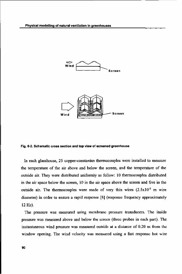
Physical modelling of natural ventilation in greenhouses
Wind
Screen
c> Wind
(h 001 p
Screen
Fig. 6-2. Schematic cross section and top view of screened greenhouse
In each glasshouse, 25 copper-constantan thermocouples were installed to measure
the temperature of the air above and below the screen, and the temperature of the
outside air. They were distributed uniformly as follow: 10 thermocouples distributed
in the air space below the screen, 10 in the air space above the screen and five in the
outside air. The thermocouples were made of very thin wires (2.5x10"5 m wire
diameter) in order to ensure a rapid response [8] (response frequency approximately
12 Hz).
The pressure was measured using membrane pressure transducers. The inside
pressure was measured above and below the screen (three probes in each part). The
instantaneous wind pressure was measured outside at a distance of 0.20 m from the
window opening. The wind velocity was measured using a fast response hot wire
90
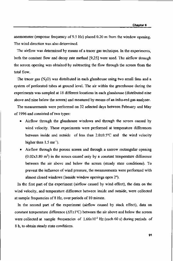
^ ^ _ _ _ Chapter 6
anemometer (response frequency of 9.5 Hz) placed 0.20 m from the window opening.
The wind direction was also determined.
The airflow was determined by means of a tracer gas technique. In the experiments,
both the constant flow and decay rate method [9,25] were used. The airflow through
the screen opening was obtained by subtracting the flow through the screen from the
total flow.
The tracer gas (N20) was distributed in each glasshouse using two small fans and a
system of perforated tubes at ground level. The air within the greenhouse during the
experiments was sampled at 18 different locations in each glasshouse (distributed nine
above and nine below the screen) and measured by means of an infra-red gas analyser.
The measurements were performed on 32 selected days between February and May
of 1996 and consisted of two types:
• Airflow through the glasshouse windows and through the screen caused by
wind velocity. These experiments were performed at temperature differences
between inside and outside of less than 2.0±0.5°C and the wind velocity
higher than 1.5 ms"1).
• Airflow through the porous screen and through a narrow rectangular opening
(0.02x3.80 m2) in the screen caused only by a constant temperature difference
between the air above and below the screen (steady state conditions). To
prevent the influence of wind pressure, the measurements were performed with
almost closed windows (leeside window openings open 2°).
In the first part of the experiment (airflow caused by wind effect), the data on the
wind velocity, and temperature difference between inside and outside, were collected
at sample frequencies of 8 Hz, over periods of 10 minute.
In the second part of the experiment (airflow caused by stack effect), data on
constant temperature difference (AT±1°C) between the air above and below the screen
were collected at sample frequencies of 1.66xl0"2 Hz (each 60 s) during periods of
8 h, to obtain steady state conditions.
91
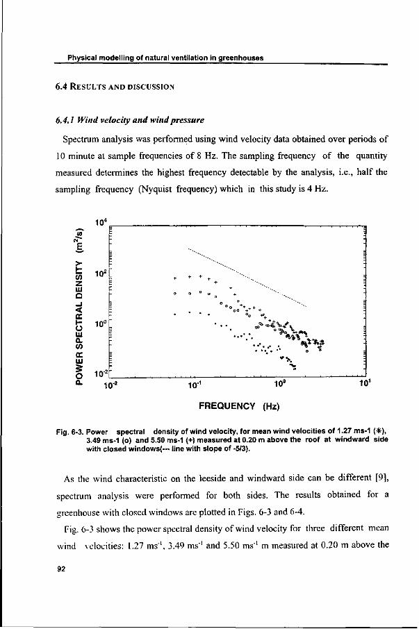
Physical modelling of natural ventilation in greenhouses
6.4 RESULTS AND DISCUSSION
6.4.1 Wind velocity and wind pressure
Spectrum analysis was performed using wind velocity data obtained over periods of
10 minute at sample frequencies of 8 Hz. The sampling frequency of the quantity
measured determines the highest frequency detectable by the analysis, i.e., half the
sampling frequency (Nyquist frequency) which in this study is 4 Hz.
104
^^ (0 rv**
E *-"' >-l -
z UJ Q - 1 < CE
O UJ Q. V)
UJ 5 o
102
E :
Ë
r
10°
KT2
-
-
' • . . .
+ + + + "'--. +• " ' - - . ,
+• "~--., o 0 ° o + ~~-,
0
• • . . * + • • • • • °o * %
TT *».
•s .
' ' ' ' = ; -" = : : ; -
! _
\
[ -
KT3 10"1 10°
FREQUENCY (Hz)
101
Fig. 6-3. Power spectral density of wind velocity, for mean wind velocities of 1.27 ms-1 ( * ) , 3.49 ms-1 (o) and 5.50 ms-1 (+) measured at 0.20 m above the roof at windward side with closed windows(— line with slope of -5/3).
As the wind characteristic on the leeside and windward side can be different [9],
spectrum analysis were performed for both sides. The results obtained for a
greenhouse with closed windows are plotted in Figs. 6-3 and 6-4.
Fig. 6-3 shows the power spectral density of wind velocity for three different mean
wind velocities: 1.27 ms"1, 3.49 ms"1 and 5.50 ms"' m measured at 0.20 m above the
92
roof on the windward side.
Chapter 6
In 10" _
>-H (/) Z UJ Q
Ê I
102
< cc h -
UJ 1 0 ° Q. W CC UJ
o OL 10*
10*
° ° <p \
10 1 10°
FREQUENCY (Hz)
101
Fig. 6-4. Power spectral density of wind velocity for mean wind velocities of 0.52 IDS'' ( * ) , 2.44 ms"1 (o) and 3.49 ms"1 (+) measured at 0.20 m above the roof at leeside with closed windows (— line with slope of -5/3).
The corresponding power spectral density of wind velocity measured on the leeside
(mean wind velocities 0.52 ms ' , 2.24 ms"' and 3.37 ms"' measured at 0.20 m above
the roof on the leeside) are shown in Fig. 6-4.
The situations represented in Fig. 6-3 and 6-4 both exhibit a region in which the
power spectral density is proportional to the frequency to the power -5/3 which is in
accordance with Kolmogorov's rule. A similarity can also be observed between the
power spectrum of wind velocity measured on the windward side and on the leeside.
In both, the main peak of power spectral density of the fluctuations occurs at
frequencies below 0.1-0.2 Hz, and for frequencies higher than l Hz there is no
93
Physical modelling of natural ventilation in greenhouses
significant contribution, i.e. low frequencies are dominant in the wind field. The fact
that main energetic eddies of wind velocity occur in this range of lower frequencies, is
supported by the studies of Kaimal et al. [26] and Bot [8].
Parameter Y can be calculated from Eqn (9) together with values of power spectral
density and frequency taken from Figs. 6-3 and 6-4. The surface roughness length z0
used in the calculations was 0.04 m [22] and the results are shown in Table 6-1. These
results show the importance of wind fluctuations (turbulence) on the total wind
pressure and that the turbulence contribution can reach 55% of the total.
TABLE 6-1. Mean wind velocity and parameter Y [Eqn (9)]
uw [ms"1]
0.52 1.27 2.24 3.37 3.49 5.50
Y= =l+/(F(n),üw,n)
1.13 1.13 1.39 1.48 1.48 1.52
6.4.2 Airflow through porous screens and openings
For airflow caused only by constant temperature differences (i.e., for quasi-steady
conditions (9Q/ôt«0) and pw»0) values are presented in Figs. 6-5 and 6-6.
Fig. 6-5 shows the experimental values of airflow through the screen and the values
predicted by Eqns (1) and (2) (l/cc2«0 [18]) versus temperature difference across the
screen.
94
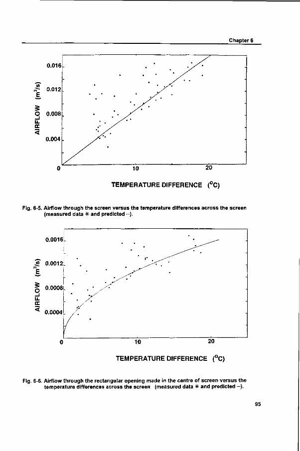
Chapter 6
0.016
~* J 2 0.012
5 O 0.008 _J LL CC < 0.004
.
•
•
•' ' /
/ •
• \ s '
/ / ' '
,/ -
-
•
•
10 20
TEMPERATURE DIFFERENCE (°C)
Fig. 6-5. Airflow through the screen versus the temperature differences across the screen (measured data * and predicted - ) .
0.0016
« 0.0012L m
E
0.0008L Li.
cc I
0.0004
10 20
TEMPERATURE DIFFERENCE (°C)
Fig. 6-6. Airflow through the rectangular opening made in the centre of screen versus the temperature differences across the screen (measured data * and predicted —).
95
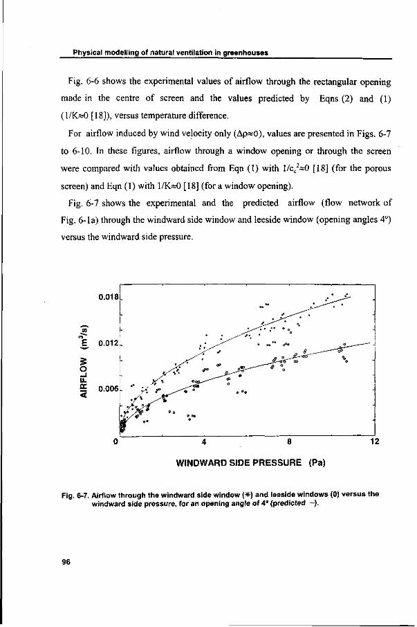
Physical modelling of natural ventilation in greenhouses
Fig. 6-6 shows the experimental values of airflow through the rectangular opening
made in the centre of screen and the values predicted by Eqns (2) and (1)
(1/K~0 [18]), versus temperature difference.
For airflow induced by wind velocity only (Ap«0), values are presented in Figs. 6-7
to 6-10. In these figures, airflow through a window opening or through the screen
were compared with values obtained from Eqn (1) with l/cc2»0 [18] (for the porous
screen) and Eqn (1) with 1/K*0 [18] (for a window opening).
Fig. 6-7 shows the experimental and the predicted airflow (flow network of
Fig. 6-la) through the windward side window and leeside window (opening angles 4°)
versus the windward side pressure.
0.018
4 8
WINDWARD SIDE PRESSURE (Pa)
12
Fig. 6-7. Airflow through the windward side window (*) and leeside windows (0) versus the windward side pressure, for an opening angle of 4° (predicted —).
96
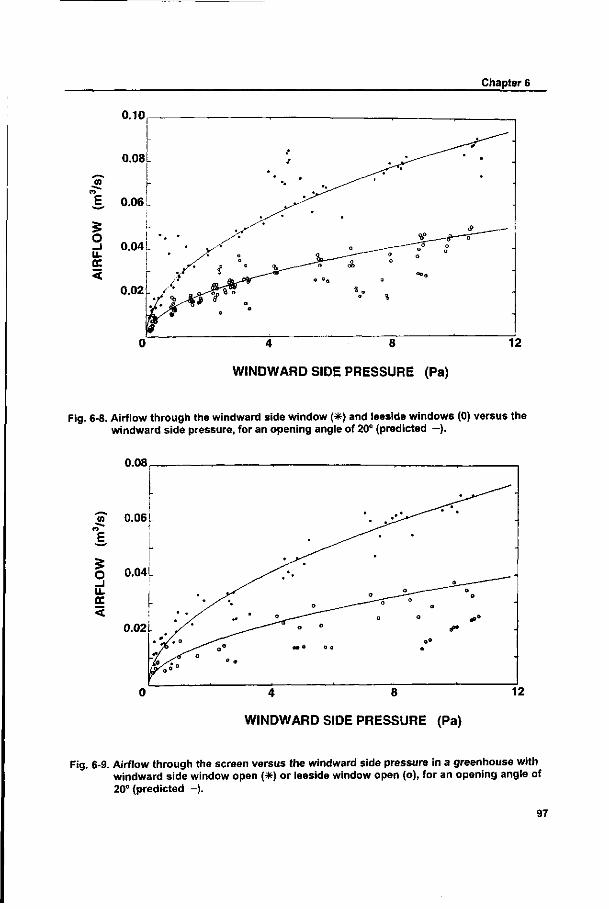
Chapter 6
0.10
4 8
WINDWARD SIDE PRESSURE (Pa)
12
Fig. 6-8. Airflow through the windward side window (*) and leeside windows (0) versus the windward side pressure, for an opening angle of 20° (predicted - ) .
0.08
4 8
WINDWARD SIDE PRESSURE (Pa)
Fig. 6-9. Airflow through the screen versus the windward side pressure in a greenhouse with windward side window open (*) or leeside window open (o), for an opening angle of 20° (predicted - ) .
97
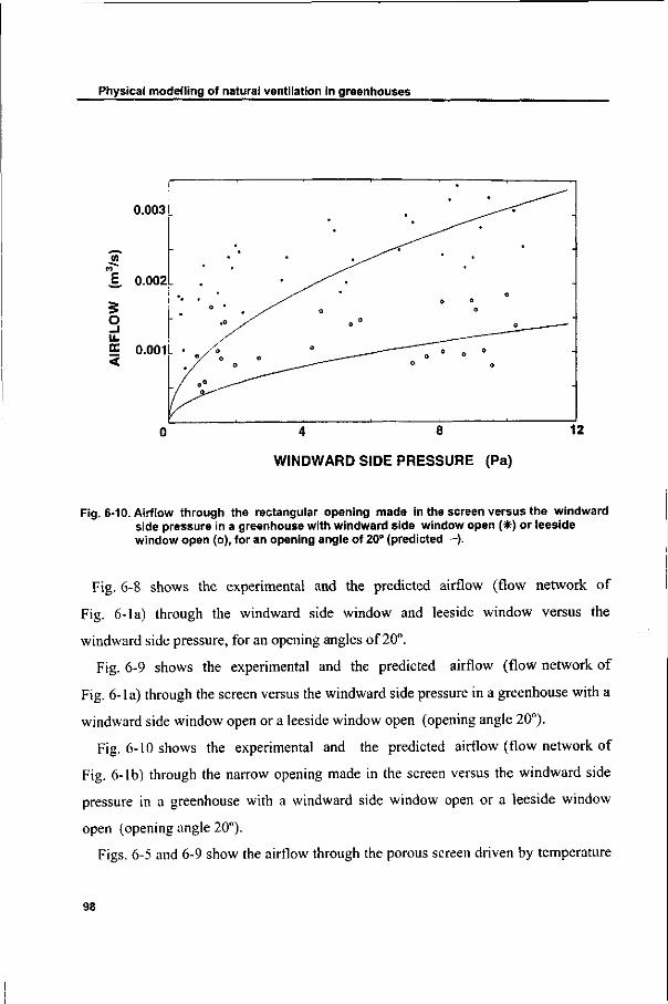
Physical modelling of natural ventilation in greenhouses
4 8
WINDWARD SIDE PRESSURE (Pa)
Fig. 6-10. Airflow through the rectangular opening made in the screen versus the windward side pressure in a greenhouse with windward side window open (*) or leeside window open (o), for an opening angle of 20° (predicted - ) .
Fig. 6-8 shows the experimental and the predicted airflow (flow network of
Fig. 6-la) through the windward side window and leeside window versus the
windward side pressure, for an opening angles of 20°.
Fig. 6-9 shows the experimental and the predicted airflow (flow network of
Fig. 6-la) through the screen versus the windward side pressure in a greenhouse with a
windward side window open or a leeside window open (opening angle 20°).
Fig. 6-10 shows the experimental and the predicted airflow (flow network of
Fig. 6-lb) through the narrow opening made in the screen versus the windward side
pressure in a greenhouse with a windward side window open or a leeside window
open (opening angle 20°).
Figs. 6-5 and 6-9 show the airflow through the porous screen driven by temperature
98
Chapter 6
difference and by the wind field respectively and they exhibit two different flow
regimes: the Darcy flow regime (Fig. 6-5) and the Forchheimer flow regime (Fig. 6-9).
These findings are supported by the work of Bear and Bachmat [27] and Bailey [2].
For Reynolds numbers (Re=puK1/2/u) smaller than unity the airflow is proportional to
the driving potential, which is the case for airflow induced by the usual range of
temperature differences between greenhouses and the ambient air (AT<25°C). For
Reynolds numbers greater than unity a quadratic term of airflow must be added
(Forchheimer flow regime) which is the case for flows induced by wind velocities
above 0.25 ms"1.
The experimental airflow values were compared with the equivalent values
predicted with the model. The differences obtained are always less than 20%, except
for Fig. 6-10. The larger scatter presented in this figure is due to the fact the airflow
through the slit was obtained by subtracting the flow through the screen from the total
flow. As the difference is small the error become relatively large.
6.5 CONCLUSIONS
1. The main energetic eddies responsible for the air exchange caused by turbulent
wind velocity were found in the frequency range below 0.1-0.2 Hz.
2. The turbulent wind velocity was estimated to be between 13% and 52% of mean
wind velocity, which means that it plays an important role in the total wind pressure.
3. The airflow through a porous screen (highly porous media) is described by the
Forchheimer's equation. However, for an airflow driven by the usual range of
temperature differences between greenhouses and the ambient air, the quadratic term
of airflow can be neglected, such that the equation can be reduced to the Darcy
law.
4. The airflow through screens and openings predicted by the theoretical approach
agree reasonable well with the experimental values, difference between them being
less than 20%, in general.
99
Physical modelling of natural ventilation in greenhouses
6.6 REFERENCES
[1] Morris L. G. and Neale F. E 1954. The infra-red carbondioxide gasanalyzer and
its use in greenhouse research. National Institute of Agricultural Engineering report,
Silsoe, United Kingdom
[2] Bailey B. J. 1978. Glasshouse thermal screens: air flow through permeable
materials. Departmental Note no. DN/G/859/04013. National Institute of Agricultural
Engineering, Silsoe, United Kingdom
[3] Bailey B. J. and Cotton R. F. 1980. Glasshouse thermal screens: influence of
single and double screens on heat loss and crop environment. Departmental Note no.
DN/G/982/04013. National Institute of Agricultural Engineering, Silsoe, United
Kingdom
[4] Silva A. M., Miguel A. F. and Rosa R. 1991. Thermal radiation inside a single
span greenhouse with a thermal screen. Journal of Agricultural Engineering Research,
49, 285-298
[5] Kosmos S .R., Riskowski G. L. and Christianson L. L. 1993. Force and static
pressure resulting from airflow through screens. Transactions of ASAE, 36, 1467-
1472
[6] Okada M. and Takakura T. 1973. Guide and data for greenhouse air
conditioning. 3: Heat loss due to air infiltration of heated greenhouses. Journal of
Agricultural Meteorology (Tokyo), 28, 223-230
[7] Kozai T. and Sase S. 1978. A simulation of natural ventilation for a multi-span
greenhouse. Acta Horticulturae, 87, 39-49
[8] Bot G. P. A. 1983. Greenhouse climate: from physical processes to a dynamic
model, Ph.D. Dissertation, Agricultural University of Wageningen, The Netherlands
[9] De Jong T. 1990. Natural ventilation of large multi-span greenhouses, Ph.D.
Dissertation, Agricultural University of Wageningen, The Netherlands
[10] Montero J. I., Anton A., Arnijas A. and Biel C. 1990. Natural ventilation in
polyethylene greenhouses with and without shading screens. Proceedings of the
100
Chapter 6
international seminar and British-Israel workshop on greenhouse technology, Bet
Dagan Israel, 65-71.
[11] Fernandez J. E. and Bailey B. J. 1992. Measurements and prediction of
greenhouse ventilation rates. Agricultural and Forest Meteorology , 58, 229-245
[12] van't Ooster A. 1994. Using natural ventilation theory and dynamic heat balance
modelling for real time prediction of ventilation rates in naturally ventilated livestock
houses. Ag. Eng. 94 Milano, Report N.94-C-012
[13] Boulard T., Meneses J. F., Mermier M. and Papadakis G. 1996. The
mechanisms involved in the natural ventilation of greenhouses. Agricultural and
Forest Meteorology, 79, 61-77
[14] Balemans L. 1989. Assessment of criteria for energetic effectiveness of
greenhouse screens Ph.D. Dissertation. University of Ghent, Belgium
[15] Okushima L., Sase S. and Nara M. 1989. A support system for natural
ventilation design of computational aerodynamics. Acta Horticulturae, 248, 129-134
[16] Ouwerkerk E. N. J., Voskamp J. P. and Aliskan Y. 1994. Climate simulation
and validation for an aviary system for laying hens, Ag.Eng. 94 Milano, Report N.94-
C-063
[17] Mistriotis A., Bot G. P. A., Picuno P. and Scarascia-Mugnozza G. 1997.
Analysis of the efficiency of greenhouse ventilation using computational fluid
dynamics, Agricultural and Forest Meteorology , 85, 217-228
[18] Miguel A. F., Van de Braak N. J., Silva A. and Bot G. P. A. 1998. Forced fluid
motion through openings and pores, Building and Environment (in press).
[19] Miguel A. F., Van de Braak N. J., Silva A. and Bot G. P. A. 1998. Analysis of
air exchange induced by fluctuating external pressures in enclosures, Building and
Environment (in press).
[20] Miguel A. F., Van de Braak N. J., Silva A. and Bot G. P. A. 1997. Analysis of
the airflow characteristics of greenhouse screening materials, Journal of Agriculture
Engineering Research 67, 105-112
101
Physical modelling of natural ventilation in greenhouses
[21] Tennekes H. and Lumley J. L. 1972. A first course in turbulence. MIT Press,
USA
[22] Eurocode ENV 1991-2-4. 1995. Basis of design and action on structures: Wind
action.
[23] Turkey J. W. 1950. The sampling theory of power spectrum estimates.
Symposium on Application of Autocorrelation Analysis to Physical Problems,
Washington, Office Naval Research, 47-67
[24] Clarke R. M. 1970. Observational studies in the atmospheric boundary layer.
Quarterly Journal Royal Meteorology Society, 96, 91-114
[25] Sherman M. H. 1990. Tracer-gas techniques for measuring ventilation in a single
zone. Building and Environment, 25, 365-373
[26] Kaimal J. C , Wyngaard J. C , Izumi Y. and Coté O. R. 1972. Spectral
Characteristics of surface-layer turbulence. Quarterly Journal Royal Meteorology
Society, 98, 563-589
[27] Bear J. and Bachmat Y. 1990. Theory and applications of transport phenomena
in porous media, Kluwer Academic Publishers, USA
[28] Peixoto J. P. and Oort A. 1992. Physics of climate, American Institute of
Physics, New York, USA
6.7 APPENDIX
Wind-induced external pressure
For a quasi-steady flow, we can write the j-direction momentum equation (Navier-
Stokes equation) as
pu(au/ôj)=-ap/5j+n(a2u/5j2) (A. I )
The wind is a turbulent airflow characterised by fluctuations of the physical
quantities such as velocity and pressure. The turbulent fluctuations of these variables
can be described by resorting to statistical methods. Using the Reynolds
102
Chapter 6
decomposition method, the instantaneous quantity at time t can be written as the sum
of a mean component (") and a fluctuating component ('). For velocity
uw=ûw + u'w (A.2)
with
ûw =x"' Juw dt
where x is longer than the period of any significant fluctuation but is much shorter
than any mean flow time scale and uw is the wind velocity.
Substitution of Eqn (A.2) into (A.l) provides
püw (5ûw/dj)=-apw/dj+uCÖ2üw /Sj2)-pd(u'wu'w )/5j (A.3)
where the third term on the right hand side represents the extra shear stress brought
about by turbulent momentum transport.
Integrating the previous equation over j-direction, we obtain
p w =0 .5p<- (p Ôûw/ôj-0.5p<u'w)+ra (A.4)
where ra is the constant of integration.
If a situation without wind is considered (ïïw = u^=0) and pw=0. Thus, TU must be
zero and
pw=0.5pü^-(p anw/5j-0.5pu'wu^) (A.5)
In the lower boundary layer of the atmosphere [28]
ôïïw/ôj=u7(Kh) (A.6)
then, Eqn (A.5) becomes
p w = 0 . 5 p ( ü i + u ; x )-p[cwf,/2ïïw/(Kh)] (A.7)
with
CwfKuVlIJ2
where cwf is the friction coefficient, h the height above the ground, u* the friction
velocity and K the von Karman constant.
If the viscosity effect is neglected (pcwf1/2/(ic h)«0), Eqn (A.7) can be reduced to a
103
Physical modelling of natural ventilation in greenhouses
relationship postulated and supported by experiments carried out by Bot [8] and de
Jong [9].
6.8 NOMENCLATURE
A
cc
Ckl
Cwf
s F<»>
g
h
H
K
L
n
P
Po
Pst
Pw
Q
rn
T
u
* u
V
area [m2]
coefficient accounting for convective effect
Kolmogorov's constant (~Q . 5)
friction coefficient
turbulent kinetic energy constant («0 . 09)
power spectral density [mV1]
gravitational acceleration [ms'2]
height [m]
characteristic depth [m]
permeability [m2]
characteristic length [m]
frequency [Hz]
pressure of air [Pa]
mean absolute pressure of air in enclosure [Pa]
stack pressure [Pa]
wind pressure [Pa]
airflow [mV]
turbulent kinetic energy dissipation rate [mV3]
absolute temperature [K]
fluid velocity [m3m"2s"']
friction velocity [ms"1]
volume [m3]
104
Chapter 6
Y inertial factor
z height [m]
z0 surface roughness length [m]
Greek symbols
ß 8
X
K
M
71
P
Y
coefficient of thermal expansion [K1]
porosity
time [s]
von Karman's constant («0 .4)
dynamic viscosity [Nsm"2]
constant («3.1416)
density [kg m"3]
wind pressure coefficient
Subscripts
fr
i
1
rmsw
s
st
w
flow field
inside
larger length
root mean square wind velocity
smaller length
stack
wind
105
106
7. Free convection heat transfer in screened greenhouses +
Abstract: Free convection heat transfer between heating pipes and air, horizontal
screen and air and inner roof surface and air was studied experimentally in twin-span
glasshouses, under constant heat flux conditions. Among others results, equation
coefficients between Nusselt and Rayleigh numbers are presented for the inner surface
of the greenhouse roof, screen surfaces and heating pipes. Special attention is given to
the influence of the location of the heating pipes relative to the screen, as well as the
presence of a crop, upon the convective heat transfer between different surfaces and
air. The equation coefficients obtained in this work are between 2% and 75% greater
than the equivalent equation coefficients found for smooth plates and cylinders by
other authors.
7.1 INTRODUCTION
Free convection heat transfer is an important mechanism of energy transport
between the surfaces of a greenhouse and the enclosed air [1-5]. However, little
information and data on this subject are currently available in the literature and what
there is, is almost exclusively devoted to unscreened greenhouses.
Despite the fact that the use of screens in greenhouses provides a simple and
successful way of avoiding night-time heat loss and controlling solar radiation
entering the greenhouse, studies on convective heat transfer have been performed
almost exclusively in greenhouses without screens. As far as is known only one study
was made by Stoffers [6] in 1984 for the purpose of determining convective heat
transfer in greenhouses divided by a horizontal screen. It is believed that a better
knowledge of the heat-transport processes will bring important improvements in
greenhouse modelling.
+ J. Ag. Engng. Research (in press)
Free convection heat transfer in screened greenhouses
The main object of this research was to produce information about free convective
heat transfer inside screened greenhouses. To achieve this, experiments were
performed in three twin-span glasshouse compartments having an airtight screen
placed horizontally between the ground and the roof, in each of these compartments.
The situations studied included the presence and the absence of an artificial crop, and
the heating pipes positioned at two different heights. Thus, the influence of the crop
and the location of the heating pipes on convective heat transfer was investigated.
Equation coefficients are presented for convective heat-transfer coefficients between
the inner surface of the greenhouse roof and air, screen surfaces and air, and heating
pipes and air.
7.2 THEORETICAL BACKGROUND
Consider a multi-span greenhouse with a screen (partition) between the ground and
the roof (two-zone enclosure), with adiabatic (highly insulated) ground and side walls.
The enclosure is heated by pipes placed just above the ground. The mode whereby
energy is transferred from the heating pipes to the outside of the greenhouse involves
three different processes: conduction, convection and radiation. The energy from the
heating pipes arrives by convection and radiation at the lower screen surface. The
energy is conducted through the screen, arrives both by convection and radiation at the
roof surface, where it is conducted through the glass and dissipated in the outside of
the greenhouse cover by convection and radiation.
Convective and radiative heat flux density are related to the heat flux generated by
the heating pipes Qe by
Qe=Qca+Qm (1)
where Qm represents the radiation heat flux density from the hot surface of the pipes to
the environment and Qca the convective heat flux density from the surface of the pipes
to the fluid.
108
Chapter 7
7.2.1 Heat transfer by convection
The convective heat transfer is defined according to [7]
Qca=o(T-T«) (2)
where a represents the convective heat transfer coefficient, T the surface temperature
and T . the temperature of the free stream fluid.
It was soon established that a is not a constant but a function of many parameters
describing the heat transfer process. Since the work of Fishenden and Saunders [8]
convective heat-transfer coefficient is expressed as a relation between the
dimensionless Nusselt number (Nu) and the Rayleigh number (Ra) as
Nu=c0Ran (3)
In Eqn (3)
Nu=cd/A, (4)
Ra=Gr Pr (5)
Gr=ß(T-TJgl3/v2 (6)
and
Pr=v/A (7)
where ß represents the volumetric coefficient of expansion of the air, g gravitational
acceleration, 1 a characteristic dimension, v kinematic viscosity, X thermal
conductivity, A thermal diffusivity, and Gr and Pr the Grashof and Prandtl numbers,
respectively.
For experiments performed under constant heat flux conditions, results can also be
presented in terms of a modified Grashof number [9]
Nu=c*(Gr*Pr)b (8)
with
Gr*=GrNu=ßQcagl4/(^v2) (9)
c*=c01/(1+n) (10)
b=n/(l+n) (11)
109
Free convection heat transfer in screened greenhouses
For experiments performed under constant heat flux conditions Eqn (8) can be
advantageous because it is dependent on convective heat flux instead of temperature
difference.
From Eqn (3) together with Eqns (4)-(7) it can be deduced that
a=ca(T-T.)n (12)
and Eqn (2) rewritten as
Q c a=c a(T-TX' (13)
with
Ca={c0/[l(1/n,-3vA/(ßg^1/n)]n} (14)
It should be noted that the fluid properties included in Eqns (3) to (14) should be
measured for the mean temperature between the surface and the free stream fluid. The
characteristic dimension 1 depends on the geometry of the system considered. For
enclosures, Holman [7] suggests that the distance between surfaces in the direction of
the air flow perpendicular to horizontal plates (ground, partitions) under study should
be chosen as the characteristic dimension. For a horizontal cylinder (heating pipes), 1
should be taken as the diameter. For a greenhouse roof, Stoffers [6] suggests that the
length of the roof under study should be chosen as the characteristic dimension.
7.2.2 Flow characteristics criterion
The coefficients c0 and n can be calculated by experiment or theoretically [7].
Generally, the constant c0 is presented as dependent on the geometry and orientation of
the surface under consideration, and the exponent n dependent only on the convection
regime.
There are three flow regimes, which can be considered: initial, laminar and turbulent
regime. The initial regime is characterised by purely conductive heat transfer. In the
laminar regime a circulation flow starts. This regime is characterised by convective
currents parallel to the surface. Transport of momentum depends on the transport by
110
Chapter 7
diffusion between the fluid layers. A turbulent regime appears when the flow becomes
unstable and vortices arise. This regime is characterised by fluctuations in velocity,
temperature and pressure.
The criterion for identifying the flow regime is the Rayleigh number. For plates in
enclosed spaces Hollands et al. [10] suggest: 1700 < Ra < 3500 (initial);
3500 < Ra < 106 (laminar); and Ra > 106 (turbulent). For horizontal cylinders Holman
[7] suggests: 103 < Ra < 109 (laminar) and Ra > 109 (turbulent).
In this study, coefficients c0, c", n and b were determined experimentally, on the
basis of the relations given by Eqns (3), (8) and (12), for the case of free convective
heat transfer between heating pipes and air, between the upper and lower surfaces of
the screen and air, and between the inner surface of the roof and air.
7.3 EXPERIMENTAL ARRANGEMENT
Experiments were conducted in three twin-span glasshouse compartments (Fig. 7-1),
each one with the following dimensions: eaves height 4.5 m, roof angle 22°, width
4.1 m and length 6.6 m.
The walls were made of 0.10 m thick insulating panels and the soil surface was
covered with 0.05 m thick polystyrene foam insulating layers. Polyethylene film was
used between the soil surface and the polystyrene foam in order to prevent the
evaporation of soil water. Both walls and soil surfaces in contact with air within the
greenhouse were covered with aluminium. The compartments roof was made of single
glass with characteristics similar to commercial greenhouses (thickness 4 mm and
thermal conductivity 0.88 Wirf'K;1).
Inside each compartment an air-tight aluminised screen (reflectivity to thermal
radiation 85%) was assembled horizontally between the ground and the roof at a
height of 2.90 m above the ground. This screen possessed roughness, as do the screens
used in greenhouses.
111
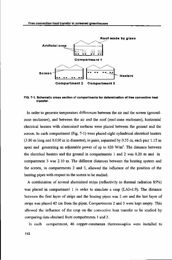
Free convection heat transfer in screened greenhouses
Roof made by g lass
Artif icial crop
Compar tment 1
Screen Heaters
Compar tment 2 Compar tment 3
FIG. 7-1. Schematic cross section of compartments for determination of free convective heat transfer.
In order to generate temperature differences between the air and the screen (ground-
zone enclosure), and between the air and the roof (roof-zone enclosure), horizontal
electrical heaters with aluminised surfaces were placed between the ground and the
screen. In each compartment (Fig. 7-1) were placed eight cylindrical electrical heaters
(3.80 m long and 0.050 m in diameter), in pairs, separated by 0.35 m, each pair 1.15 m
apart and generating an adjustable power of up to 820 W/m2. The distance between
the electrical heaters and the ground in compartments 1 and 2 was 0.20 m and in
compartment 3 was 2.10 m. The different distances between the heating system and
the screen, in compartments 2 and 3, allowed the influence of the position of the
heating pipes with respect to the screen to be studied.
A combination of several aluminised strips (reflectivity to thermal radiation 85%)
was placed in compartment 1 in order to simulate a crop (LAI«1.9). The distance
between the first layer of strips and the heating pipes was 2 cm and the last layer of
strips was placed 42 cm from the pipes. Compartments 2 and 3 were kept empty. This
allowed the influence of the crop on the convective heat transfer to be studied by
comparing data obtained from compartments 1 and 2.
In each compartment, 46 copper-constantan thermocouples were installed to
112
Chapter 7
measure the temperature of the air, heating pipes, screen and inner surface of the roof.
They were distributed as follows: six distributed on the roof, ten in the air space above
the screen, twelve distributed on the screen, ten in the air space below the screen and
eight on the heating pipes. In order to make sure that the thermocouples sensed the
correct temperature of the heating pipes, the screen surface and the inner surface of the
roof, they were bonded to the surface and covered with a thin layer of material with
the same optical properties as the surface. To reduce conductive heat flux, the
thermocouples were made of thin wires (each wire 0.025 mm in diameter). They were
connected to the surface along their length (»20 cm) to ensure that the sensing point
was at the surface temperature.
Net radiometers (spectral range 0 to 60 (im) were placed above and below the
screen to measure the radiative heat losses. The radiometers were positioned in such a
way that all radiation fluxes incident to or leaving both the screen surfaces and the
inner side of the roof could be detected. The net thermal radiation at the heating pipes
was estimated using the model developed by Silva et al. [11].
7.4 DESCRIPTION OF EXPERIMENTS
Measurements were made at night between 27 October 1995 and 4 December 1995,
in order to exclude the effects of short wave radiation on the measurements. The three
compartments were kept "dry", i.e. without vapour condensation on the screen surface,
inner surface of the walls or inner surface of the roof.
The thermocouples and net radiometers were scanned by a data-logging system at
intervals of 30 s and for periods of time of 12-13 h to record data during the steady
state periods. As the temperature inside the greenhouse changes as a result of changes
in the outside temperature, the criterion used to evaluate steady state conditions was a
quasi-constant temperature difference (AT±1°C) between the surfaces and the air.
In each compartment the heat flux supplied by the electrical heaters was the only
113
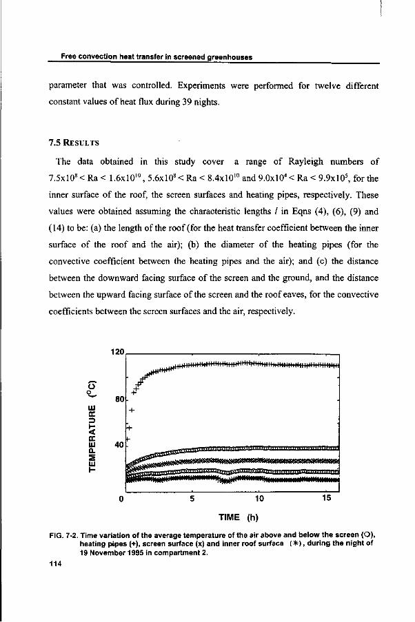
Free convection heat transfer in screened greenhouses
parameter that was controlled. Experiments were performed for twelve different
constant values of heat flux during 39 nights.
7.5 RESULTS
The data obtained in this study cover a range of Rayleigh numbers of
7.5xl08 < Ra < 1.6x10'°, 5.6xl08 < Ra < 8.4x10'° and 9.0xl04 < Ra < 9.9xl05, for the
inner surface of the roof, the screen surfaces and heating pipes, respectively. These
values were obtained assuming the characteristic lengths / in Eqns (4), (6), (9) and
(14) to be: (a) the length of the roof (for the heat transfer coefficient between the inner
surface of the roof and the air); (b) the diameter of the heating pipes (for the
convective coefficient between the heating pipes and the air); and (c) the distance
between the downward facing surface of the screen and the ground, and the distance
between the upward facing surface of the screen and the roof eaves, for the convective
coefficients between the screen surfaces and the air, respectively.
u o Ol cc
< OC uu o. s LU
120
80 /
^ j H * * * * * * * f-H iH4 ii " ii iHi ii IHHH-TH MMI M H IHI ii ii M M H-ii i mi
TIME (h)
FIG. 7-2. Time variation of the average temperature of the air above and below the screen (O), heating pipes (+), screen surface (x) and inner roof surface ( * ) , during the night of 19 November 1995 in compartment 2.
114
Chapter 7
The conductive heat losses through the insulated ground and walls were determined
by calculations from the thermal properties of the materials given by the
manufacturers together with the measurement of the temperature distribution. The
radiative flux inside the compartments was measured experimentally using
radiometers. These fluxes represent a maximum of 1.6% (conductive heat loss) and
10.3% (radiative flux) of the heat generated by the heating pipes. That is, the
minimum convective heat flux was always greater than 88% of the supplied heat flux.
Therefore, inaccuracies in the corrections for conductive and radiative terms only
cause a small error in the convective term.
As mentioned previously, the experiments were performed over a period of several
hours to ensure that a steady state was reached. Figure 7-2 shows the variation over
time of the average temperature of the air (above and below the screen), screen surface
temperature and inner roof surface temperature for the night of 19 November 1995 in
compartment 2. It will be noted that the temperature difference between the surfaces
and the air remained constant after approximately 8 h, which means that a steady state
condition had been reached. Similar results were obtained for the other test nights, and
the steady state was always reached within 10 h of the beginning of the experiment.
Figures 7-3 to 7-5 present the convective heat flux (Qca) versus the temperature
difference (T-TJ, between the inner surface of the roof and the air, between upper and
lower facing surfaces of the screen and the air, and between the heating pipes and the
air, respectively.
According to Figs. 7-4 and 7-5, the distance of heating pipes from the downward
facing screen surface do not influence the convective heat transfer between lower
surface of the screen and air, and between heating pipes and air. The presence of the
crop increases the convective heat flux and hence the convective heat-transfer
coefficient by approximately 16% between the heating pipes and the air.
The data, presented in Figs. 7-3 to 7-5, can be fitted with Eqn (13) and coefficients
ca and n found by logarithmic regression analysis. These coefficients are presented in
115
Free convection heat transfer in screened greenhouses
Table 7-1.
E
x 3
< UJ X UI
> o UJ > z o o
TEMPERATURE DIFFERENCE (°C)
FIG. 7-3. Convective heat flux versus the temperature difference between inner surface of roof and the air (all compartments).
E 5
x
5« LU X Ui
> O Ul > z o Ü
TEMPERATURE DIFFERENCE (°C)
FIG. 7-4. Convective heat flux versus the temperature difference between the screen [upward facing surface ( * ) and downward facing surface (O)] and the air (all compartments).
116
Chapter 7
E
x
< UJ X UJ
> H Ü Ui > z o ü
TEMPERATURE DIFFERENCE (°C)
FIG. 7-5. Convective heat flux versus the temperature difference between the heating pipes in the compartment 1 (x), 2 (+) and 3 (O) and the air.
TABLE 7-1. Coefficients c„ and n for the best fit of Eqn (13)
Inner surface of roof Upper surface of screen Lower surface of screen Heating pipes 1 Heating pipes 2 Heating pipes 3
Ca
3.02 3.24 2.17 3.37 2.99 3.03
n
0.32 0.30 0.31 0.26 0.24 0.24
r2
0.97 0.96 0.97 0.98 0.98 0.99
NDn
98 82 69 35 38 39
1 Number of fitted data
According to Table 7-1, the exponent n obtained for the screen surfaces and inner
surface of the roof is close to 1/3 (turbulent flow regime) and for the heating pipes
close to 1/4 (laminar flow regime). If it is assumed that n exponents of 1/3 and 1/4 are
117
Free convection heat transfer in screened greenhouses
the true values, then new values of ca are obtained which are slightly different from
the values found previously. The new values of ca for exponent n equal to 1/3 and 1/4
are presented in Table 7-2. From knowledge of ca and n, the convective coefficients c0
and c* can be computed from Eqns (14) and (10), and the relations between Nu and Ra
or between Nu and Gr* obtained. These relations are presented in Table 7-3.
TABLE 7-2. Coefficients c„ obtained for exponent n equal to 1/3 (turbulent flow) and 1/4 (laminar flow)
Inner surface of roof Upper surface of screen Lower surface of screen Heating pipes 1 Heating pipes 2 Heating pipes 3
2.97±0.29 3.09±0.27 2.09±0.14 3.42±0.12 2.90±0.19 2.98±0.18
1/3 1/3 1/3 1/4 1/4 1/4
TABLE 7-3. Free convective heat transfer correlations
Nu= c0 Ra° Nu=c*(Gr*Pr)b
c* b
Inner surface of roof Upper surface of screen Lower surface of screen Heating pipes 1 Heating pipes 2 Heating pipes 3
0.270±0.026 1/3 0.281±0.024 1/3 0.19U0.013 1/3 0.299±0.011 1/4 0.254±0.017 1/4 0.261±0.015 1/4
0.374±0.036 1/4 0.386±0.033 1/4 0.289±0.020 1/4 0.404±0.015 1/5 0.358±0.024 1/5 0.365±0.021 1/5
118
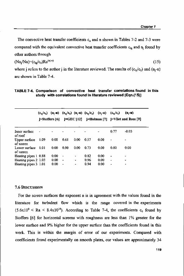
Chapter 7
The convective heat transfer coefficients ca and n shown in Tables 7-2 and 7-3 were
compared with the equivalent convective heat transfer coefficients c0j and nj found by
other authors through
(NuJ/Nu)=(c0j/c0)Ra<nJ-n> (15)
where j refers to the author j in the literature reviewed. The results of (c0j/c0) and (nj-n)
are shown in Table 7-4.
TABLE 7-4. Comparison of convective heat transfer correlations found in this study with correlations found in literature reviewed [Eqn.(15)]
(c0J/co) (nrn) (c„/c0) (nrn) (coj/c„) (nrn) (coj/c„) (nrn)
j=Stoffers [6] j=GEC [12] j=Holman [7] j=Vliet and Ross [9]
0.77 -0.03
0.80 0.00
Inner surface ofroof Upper surface 1.09 of screen Lower surface 1.01 of screen Heating pipes 1 0.88 Heating pipes 2 1.03 Heating pipes 3 1.01
-
0.00
0.00
0.00 0.00 0.00
-
0.61
0.90
---
-
0.00
0.00
---
-
0.57
0.73
0.82 0.96 0.94
-
0.00
0.00
0.00 0.00 0.00
7.6 DISCUSSION
For the screen surfaces the exponent n is in agreement with the values found in the
literature for turbulent flow which is the range covered in the experiments
(5.6xl08 < Ra < 8.4xl010). According to Table 7-4, the coefficients c0 found by
Stoffers [6] for horizontal screens with roughness are less than 1% greater for the
lower surface and 9% higher for the upper surface than the coefficients found in this
work. This is within the margin of error of our experiments. Compared with
coefficients found experimentally on smooth plates, our values are approximately 34
119
Free convection heat transfer in screened greenhouses
and 75% higher than the coefficient c0 referred to by Holman [7]. GEC [12] presents
coefficients c0 which are 10 and 39% lower than the coefficients for the screen
surfaces obtained in this study. The coefficients obtained by GEC [12] were found on
a horizontal plate of size 3.66 m x 3.66 m with application in the range
5x l0 9 <Ra<lx l0 1 2 .
The differences between convective heat transfer coefficients c0 obtained in this
study and the coefficients presented by Holman [7], Vliet and Ross [9] and GEC [12]
may partly be owing to the fact that the screen is not a smooth plate but is rough.
Rough plates transfer more heat than smooth surfaces because roughness induces extra
local convection currents.
For the inner surface of the glass the power coefficient n is in agreement with the
values found in the literature for turbulent flow, which is the range covered in the
experiments. According to Table 7-4, the coefficient c0 found in this work is 30%
greater than the value presented by Vliet and Ross [9] on a plate with an inclination
of 22° and with application in the range 104 < Ra < 106. The coefficients c0 presented
by Papadakis et al. [5] (roof with span angle 15°) and by Stoffers [6] (roof with span
angle 26°) cannot be compared directly with our results (roof with span angle 22°)
because the convective heat transfer coefficient depends on the angle of inclination
between the surface and the horizontal [13].
The exponent n for the heating pipes is in agreement with the values found in the
literature for laminar flow, the range considered in the experiments. According to
Table 7-4, for the heating pipes in compartments 2 and 3 (without artificial crop) the
coefficient c0 found in this work is approximately 2% lower than the coefficient found
by Stoffers [6] and 5% higher than the coefficient referred to by Holman [7], but both
fall within our interval of uncertainty. On the other hand, the coefficient c0 found by us
for heating pipes in compartment 1 (with artificial crop) is 22% higher than the
underlying coefficient referred to by Holman [7] and 14% higher than that referred to
by Stoffers [6].
120
Chapter 7
In the literature reviewed, the convective heat coefficients for pipes are obtained
with one or two cylinders in an "infinite space", that is, where air movement induced
by other surfaces can be disregarded. In the case of compartment 1, extra air
movement, induced by the presence of an artificial crop, influences the convective
heat transfer at pipe surfaces. This effect explains the higher values obtained in
compartment 1 compared with remaining compartments, and the similarity between
the values found in compartments 2 and 3 and the literature reviewed.
The data collected in this study cover a Rayleigh number range which is not
commonly found in heat transfer literature [7], mainly for the inner surface of the
roof and the screen surfaces. However the data obtained in these experiments is
commonly relevant to greenhouses.
7.7 CONCLUSIONS
1. The height of heating pipes above the soil surface (0.20 m and 2.10 m) did not
influence the convective heat transfer between the heating pipes and the air.
2. The distance of heating pipes from the downward facing screen surface (0.80 m
and 2.70 m) did not influence the convective heat transfer between the heating pipes
and the air and between the lower surface of the screen and the air.
3. The presence of an artificial crop (LAI« 1.9) increased the convective heat transfer
coefficient by approximately 16% between the heating pipes and the air.
4. The equations coefficient obtained in this study agree well with those presented by
Stoffers [6] for similar conditions.
5. The equation coefficients obtained in this work are between 2% and 75%
greater than the equivalent equation coefficients presented in heat transfer
literature for experiments performed on smooth plates and cylinders.
6. The differences between screen equation coefficients obtained in this study and the
equivalent equations presented by other authors can partly be attributed to the fact that
121
Free convection heat transfer in screened greenhouses
the screen is not a smooth plate but is rough.
7.8 REFERENCES
[1] Bailey B. J. 1981. The evaluation of thermal screens in glasshouse commercial
nurseries. Acta Horticulturae, 115, 663-670
[2] Bot G. P. A. 1983. Greenhouse climate: from physical process to a dynamic
model. Ph.D. Dissertation. Agricultural University of Wageningen, The Netherlands
[3] Silva A. M. 1988. A contribution to the study of the greenhouse climate: the
analysis of some processes of energy transfer (Contribuiçào para o estudo do clima de
uma estufa: estudo de alguns processos fïsicos de transferência). Ph.D. Dissertation.
University of Evora, Portugal (In Portuguese)
[4] Balemans L. 1989. Assessment of criteria for energetic effectiveness of
greenhouse screens Ph.D. Dissertation. University of Ghent, Belgium
[5] Papadakis G., Frangoudakis A. and Kyritsis S. 1992. Mixed, forced and free
convection heat transfer at the greenhouse cover. Journal of Agricultural Engineering
Research, 51, 191-205
[6] Stoffers J . A. 1984.Energy fluxes in screened greenhouses. Ag Eng 84 Cambridge,
United Kingdom
[7] Holman J. P. 1990. Heat transfer. Seventh edition. Singapore, MacGraw-Hill,
New York, USA
[8] Fishenden M. and Saunders O. A. 1957. An introduction to heat transfer.
London, Clarendon Press, United Kingdom
[9] Vliet G. C. and Ross D. C. 1974. Turbulent natural convection on upward and
downward facing inclined constant heat flux surfaces. ASME Paper 74-WA/HT-32
[10] Hollands K. G. T., Raithby G. D. and Konicek L. 1975. Correlation equations
for free convection heat transfer in horizontal layers of air and water. International
Journal of Heat and Mass Transfer, 18, 879-884
[11] Silva A. M., Miguel A. F. and Rosa R. 1991. Thermal radiation inside a single
122
Chapter 7
span greenhouse with a thermal screen. Journal of Agricultural Engineering Research,
49, 285-298
[12] GEC Heat transfer data book, 1982. Kaminsky, D. A. ed.. New York, General
Electric Company, Sect. 504.2, 1-15, USA
[13] Fujii T. and Imura H. 1972. Natural convection heat transfer from a plate with
arbitrary inclination. International Journal of Heat and Mass Transfer, 15, 755-765
7.9 NOMENCLATURE
b, c0, ca, c*, n convective coefficients
g gravitational acceleration [ms~2]
Grashof number
modified Grashof number
characteristic length [m]
Nusselt number
Prandtl number
heat flux density [Wm2]
Rayleigh number
temperature [K]
Gr
Gr*
1
Nu
Pr
Q
Ra
T
Greek symbols
a
ß
A
X
v
convective heat transfer coefficient across fluid layer [Wm'2K"']
volumetric coefficient of expansion [K"1]
thermal diffusivity [mV]
thermal conductivity [Wm'k1]
kinematic viscosity [mV1]
Subscripts
ca convective
123
Free convection heat transfer in screened greenhouses
e electrical heaters
j author in literature reviewed
rn radiation
oc free stream fluid.
124
8. FINAL DISCUSSION AND CONCLUSION
8.1 A IR INFILTRATION IN ENCLOSURES WITH PORES AND OPENINGS
In this thesis, a motion equation for porous media and openings is derived within the
principles of fluid mechanics and thermodynamics. This validity is based on several
simplifications, mainly on the assumption that the medium under study is
homogeneous on a macroscopic scale, and that deformation and loss of mass by the
solid matrix do not occur. In general terms, this description is valid to describe flow
through porous media and through non-porous media (gaps, cracks, doors, windows)
with permeability as the quantity which connects both extremes (pores and openings).
Specifically, the equilibrium state of the fluid within the porous medium, as well as
the importance of inertia effects and viscous effects on the fluid transport through the
medium, are stated and quantified.
For a porous medium at low velocities (Re<l), viscous effects (viscous resistance
force due to the momentum transfer at the matrix-fluid interface and viscous resistance
of fluid flow) are dominant. Instead, for higher velocities (Re>l) fluid flow is strong
dependent of the pore' inertial effects. For an opening, convective inertia effects are
dominant.
The motion equation, together with the mass conservation and the state equation of
gases, are used to describe air infiltration in enclosures. Airflow and internal pressures
were related to characteristics of the openings, which connect the enclosure zones, and
also to the characteristics of the enclosure and objects within the enclosure (volume,
flexibility).
For an enclosure with a large free area opening, the internal pressure response to
external pressure is oscillatory and exhibits damping. When the opening area
decreases, the damping increases. If the use of porous screen in the opening is
adopted, the internal is strongly damped and the equilibrium is reached immediately.
Final discussion and conclusion
The flexibility of enclosure envelope also affects the internal pressure response. The
increase of flexibility decreases the internal pressure amplitude and equilibrium
pressure is reached more quickly.
The essence of the present research is to provide a theory which can be applied to
practical situations. The developed approaches are therefore applied to a practical
problem, the study of screened greenhouses. Three objectives are in view:
• to provide extra information for a better characterisation of the driving potential
of the process (wind velocity, air temperature),
• to obtain easily measurable parameters which are required for the developed
approaches,
• to test the approaches proposed against real data.
A complication in the evaluation of driving potentials is the fluctuate character of
wind velocity. Most of works on fluid flow through openings and porous materials
consider only the static flow. In the present study the effect of fluctuations is included.
To clarify and to characterize the structure of fluctuations of wind velocity, a power-
spectrum analysis was performed. The frequencies of the main energetic eddies
responsible for the air exchange were obtained, being located at frequencies of around
0.1-0.2 Hz. The turbulence contribution of wind velocity to the wind pressure was also
obtained, and can reach 55% of the total pressure. These values were obtained for
mean wind velocities between 0.5 ms"1 and 5.5 ms"1 and both results are supported by
the studies of others authors.
The airflow characteristics of porous screens were input requirements of the
proposed approaches. These characteristics were identified as being permeability and
porosity, and they were obtained through relatively simple experimental procedures
(DC-pressurisation method). From the experimental data obtained, it is possible to
conclude that the screens used as thermal screens have permeabilities close
to 10"m2 and insect screens smaller than 10"8m2. Some thermal screens, mainly
woven sheet screens, can be damaged by opening and closing the screen, and
126
Chapter 8
due to this permeability can increase up to 3.5 times the original value. For a damaged
screen, airflow predicted based on permeability of a new material underestimate the
flow up to about 30%.
The approaches were tested with real data obtained in both small-scale
measurements and full-scale measurements. The predictions made agree reasonably
well with the experimental data. In general, differences between them were less than
20%.
8.2 FREE CONVECTIVE HEAT TRANSFER INSIDE A SCREENED GREENHOUSE
An experimental study on free convection heat transfer was performed in small
greenhouses with a horizontal screen. The analysis of the data obtained emphasises the
following conclusions
• the convective heat transfer coefficients between the air and the downward and
upward surface of the screen were Nu=0.191 Ra033 and Nu=0.281 Ra033,
respectively;
• the convective heat transfer coefficients between the air and the inner side of
the roof was Nu=0.270 Ra033 (roof angle 22 °);
• the position of the heating pipes in relation to the screen (0.80 m and 2.70 m)
does not seem to influence the convective heat transfer between the downward
facing surface of the screen and the air, nor between the heating pipes and the
air;
• the presence of an artificial crop seems to have an influence on the convective
heat transfer between the heating pipes and the air, for the range of Rayleigh
numbers considered in this study (9.0xl04<Ra<9.9xl05). The presence of an
artificial crop (LAI« 1.9) increases the convective heat transfer coefficient by
approximately 16%.
The equation coefficients obtained in this study are between 2% and 75% greater
than the equivalent equation coefficients found for smooth plates and cylinders by
127
Final discussion and conclusion
other authors. This may partly be owing to the fact that the screen is rough and
roughness induces extra local convective currents. Also, the presence of crop seems to
induce extra convective currents, which explain the higher convective heat transfer
between the heating pipes and the air in the compartment with crop.
Notice that, the data obtained in these experiments is not commonly found in heat
transfer literature, but is relevant to greenhouses.
8.3 FINAL REMARKS
The description presented in this study contributes to clarify some important aspects
of transport phenomena in multi-zone enclosures with permeable walls and has a wide
application.
Nowadays, the interest in predicting the behaviour of physical systems through
simulation programs is very important. These techniques are much less expensive than
small scale or full-scale experiments, allowing the simulation of a very large number
of situations in a short period of time. In order to enable an accurate simulation,
advances in transport phenomena as a base for this modelling are fundamental.
The study presented in this thesis describes the main aspects concerning the
transport phenomena in porous media and openings, which can be implemented in
simulation programs with this topic. The formulation presented was incorporated in an
existing dynamic climate model called KASPRO, developed by Zwart [1]. At present,
model predictions are compared with experimental data obtained in screened
greenhouses situated at Research Station PBG in Naaldwijk (west of the Zuid Holland
province in the Netherlands) with very promising results [2,3]. In the future, the
simulation study of greenhouse control strategies will support the climate control
management. Particularly, it will allow establishment of rules for optimal air humidity
control and energy saving strategies, combining the screen characteristics and
the percentage of screen and window aperture.
128
Chapter 8
8.4 REFERENCES
[1] Zwart H. F. de 1996. Analysing energy-saving options in greenhouse cultivation
using a simulation model. Ph.D. Dissertation, Agricultural University of Wageningen,
the Netherlands
[2] Braak N. J. van de, Swinkels G. L. A. M., Knies P. and Breuer J. J. G. 1997.
Verhoging energie-effïciëntie door verbeterde schermregeling (Higher energy
efficiency by an improved screen control). Report note P97-XX, IMAG-DLO
Wageningen, the Netherlands, [in Dutch]
[3] Braak N. J. van de, Kempkes F. L. K., Bakker J. C. and Breuer J. J. G. 1997.
Application of simulation models to optimize the control of thermal screens. ISHS 97
Conference, August of 1997, Wageningen, the Netherlands.
129

SAMENVATTING
Warmte- en stoftransport zijn verschijnselen van groot belang in diverse natuurlijke en
industriële processen, zoals klimaatbeheersing in ruimten met poreuze wanden of wanden
met openingen (gebouwen, tuinbouwkassen, enz.). In dit proefschrift worden twee
aspecten beschouwd: massatransport door poreuze materialen en openingen, en
warmteoverdracht van en naar de wand. Deze verschijnselen zijn theoretisch onderzocht
en vervolgens zijn de resultaten toegepast om een geschermde tuinbouwkas te bestuderen.
Een gedetailleerde beschrijving van het doel van het onderzoek staat in Hoofdstuk 1.
In Hoofdstuk 2 wordt geforceerde convectie door poreuze materialen en openingen
besproken. Er wordt een benadering gepresenteerd die is gebaseerd op de
impulsbehoudswet met toepassing van volumemiddeling. De resulterende benadering is
geldig voor zowel poreus als voor niet-poreus materiaal, en kan worden gebruikt in
"computational fluid dynamics" om de snelheids- en drukverdeling over het
stromingsveld te voorspellen. Er is vervolgens een nauwkeurige vereenvoudigde vorm
ontwikkeld met een klein aantal parameters en eenvoudige mathematische bewerkingen.
In Hoofdstuk 3, wordt de benadering die is ontwikkeld in Hoofdstuk 2 samen met de
massabehoudswet en de toestandsvergelijking van gassen, gebruikt om luchtuitwisseling
geïnduceerd door fluctuerende uitwendige drukken te bestuderen. De
stromingsvergelijkingen voor luchtuitwisseling in een uit meerdere compartimenten
bestaande ruimte en vergelijkingen voor de druk binnen elke compartiment met
samendrukbare lucht worden gepresenteerd.
Massatransport door permeabele materialen kan ook optreden als gevolg van
temperatuur- en concentratiegradiënten, of als resultaat van gecombineerde effecten
(gradiënten van temperatuur en concentratie samen met druk gegenereerd door wind of
mechanische middelen). Een beschrijving van gecombineerde vrije en geforceerde
convectie door poreuze media ondersteund door de basiswetten van de thermodynamica
en vloeistofmechanica, wordt gepresenteerd in Hoofdstuk 4. Met het resultaat kan de
Samenvatting
massaverandering van een poreus medium als gevolg van adsorptie en de interactie tussen
de matrix van vaste stof en de lucht of vloeistof binnen het medium worden bestudeerd.
Hoofdstuk 5 is gewijd aan de meting van luchtstromingskarakteristieken van poreuze
schermen. Negen verschillende thermische, schaduw- en insecten- schermen zijn getest
door middel van een drukverschilmethode. Hun permeabiliteit en poreuze inertiefactor
zijn bepaald overeenkomstig de Forchheimervergelijking De porositeit van het
schermmateriaal is bepaald met behulp van microscoopmetingen. Er is speciaal aandacht
geschonken aan de variatie van de luchtstromingskarakteristieken (permeabiliteit en
porositeit) als gevolg van beschadiging en door "handling".
In Hoofdstuk 6 zijn de benaderingen gepresenteerd in Hoofdstuk 2 tot 4 toegepast op
de studie van luchtuitwisseling in een geschermde tuinbouwkas. Deze studie is aangevuld
met een vermogensspectrumanalyse van de windsnelheid, om de structuur van
drukfluctuaties (turbulentie) te karakteriseren, en om de frequenties van de belangrijkste
wervels in het windveld te identificeren. De fluctuaties in de windsnelheid zijn
gerelateerd aan de gemiddelde windsnelheid, Ook de winddruk is geïnterpreteerd in
termen van de gemiddelde windsnelheid.
Hoofdstuk 7 is gewijd aan warmteoverdracht door vrije convectie in geschermde
kassen. De warmteoverdrachtscoëfficiënt aan verschillende oppervlakken is uitgedrukt
als een relatie tussen het dimensieloze Nusseltgetal en het Rayleighgetal. Vervolgens is
een experimentele studie uitgevoerd om de vrije convectie
warmteoverdrachtscoëfficiënten te bepalen (tussen lucht en verwarmingspijpen, lucht en
horizontaal scherm, en lucht en binnenste dakoppervlak) in een kas met karakteristieke
lengten dicht bij die van echte kassen. Andere praktische aspecten, zoals de invloed van
de positie van de verwarmingpijpen in relatie tot het scherm, en de aanwezigheid van een
gewas, op de convectieve warmteoverdracht tussen de verschillende oppervlakken en de
lucht, wordt besproken.
Tenslotte worden in Hoofdstuk 8 de belangrijkste conclusies van dit onderzoek
gepresenteerd en aanbevelingen gedaan voor toekomstig onderzoek.

Samenvatting
De implementatie van de gepresenteerde formulering in dynamische
kasklimaatmodellen biedt verschillende mogelijkheden om het management van het
kasklimaat te ondersteunen.

SUMARIO
A transferencia de massa e calor é urn assunto de grande importância em diversos
processos naturais e industrials como seja no controlo climätico de cavidades com paredes
permeâveis (edificios residenciais, estufas, etc.). Nesta tese dois aspectos foram
estudados: o transporte de fluidos através de poros e aberturas, e a transferencia de calor
entre as paredes interior da cavidade e o ar. Estes fenómenos foram estudados do ponto
de vista teórico, e posteriormente aplicados ao estudo de estufas com écrans. A descriçào
detalhada do objectivo deste trabalho foi feito no primeiro Capitulo desta tese.
O segundo Capitulo foi dedicado ao estudo da convecçâo forçada através de poros e
aberturas. O método denominado de "volume averaging" é aplicado à tradicional
equaçâo de balanço de momento, resultando numa equaçào valida para materiais porosos
e para aberturas. A equaçâo resolvida numericamente permite a obtençào da variaçâo
temporal e espacial dos campos da velocidade e da pressâo. A resoluçào numérica desta
equaçào nào é fâcil, e em problemas mais prâticos o detalhe da soluçâo obtida nem
sempre é necessârio. Uma forma simplificada mas précisa da equaçâo foi também
apresentada, para ser usada em casos em que apenas sào requeridos o valor media dos
campos da velocidade e da pressâo.
A equaçâo apresentada no Capitulo 2 conjuntamente com a equaçâo de conservaçâo da
massa e a equaçào de estado dos gases, foi usada para estudar trocas de ar induzidas
devido à flutuaçâo na pressâo (Capitulo 3). Baseado nestas equaçôes foi apresentado um
modelo para quantificar as trocar de ar e a pressâo numa cavidade com varias zonas.
O transporte de fluido através de materiais permeâveis pode ocorrer devido a gradientes
de pressâo originados pela velocidade do vento ou por meios mecânicos, mas também
devido a gradientes de temperatura ou de concentraçâo, ou através do efeito combinado
(gradientes de pressâo, concentraçâo, pressâo gerada pelo vento ou meios mecânicos). O
estudo da convecçâo mista através de meios porosos, baseado nas leis da termodinâmica
e da mecânica de fluidos, foi o tema do Capitulo 4. Como aplicaçâo do modelo
Sumârio
apresentado, foi estudada a variaçâo da massa de meios porosos sujeitos a diferentes
condiçôes exteriores, bem como a interacçâo matriz-fluido.
No Capitulo 5 foram obtidas experimentalmente as caracteristicas do diversos écrans
porosos ao transporte de fluido. Nove amostras de diferentes tipos de écrans foram
testados usando uma metodologia denominada de "DC-pressurization method". As suas
permeabilidade ao transporte de fluido bem como o factor de inércia dos poros foram
obtidos com base na equaçào de Forchheimer (a porosidade foi obtida com a ajuda de um
microscópio). O efeito da degradaçào do écran, devido ao seu uso, na variaçâo da
permeabilidade ao fluido e na porosidade, foi também estudada.
No Capitulo 6 os modelos apresentados no capitulo 2 a 4 foram aplicados ao estudo das
trocas de ar em estufas com écrans. O estudo contem também a analise espectral da
velocidade do vento, com o objectivo de caracterizar as flutuaçoes de pressào
(turbulência), e a identificaçâo da frequência dos principais vórtices présentes nos campos
de pressâo originados pelo vento.
O Capitulo 7 foi dedicado as transferencias convectivas de calor (convecçào natural)
no interior de estufas com écrans. Os coeficientes de transferencia de calor para diferentes
superficies foi definido como a relaçào entre os numéros adimensionais de Nusselt e de
Rayleigh. Posteriormente foi feito, um estudo experimental com o objectivo de
determinar os coeficientes de transferencia de calor entre o ar e o sistema de aquecimento,
o ar e o écran, e o ar e a face interior da cobertura da estufa. O écran usado neste estudo
apresentava alguma rugosidade tal como acontece nos écrans usados em estufas. O efeito
da posiçào do sistema de aquecimento em relaçào ao écran, bem como a presença de
vegetaçào, no coeficiente de transferencia convectiva de calor entre as diferentes
superficies e o ar, foi também estudado.
Finalmente, no Capitulo 8, foram apresentadas as principais conclusôes deste estudo,
e incluidas também algumas possiveis linhas de investigaçâo futura.
A futura implementaçâo da formulaçào apresentada neste estudo em modelos
dinâmicos, constituirâ uma ferramenta importante no estudo do clima interior de
cavidades com varias zonas.
SUMMARY
Exchange of mass and heat is a topic of great importance in diverse natural and
industrial processes as, for instance, in indoor climate control in enclosures with
permeable boundaries (residential buildings, greenhouses, etc.). In this thesis two aspects
were considered: fluid transport through pores and openings, and heat transfer between
the enclosure surfaces and the inside air. Firstly, these phenomena are examined
theoretically and subsequently they are applied to the study of screened greenhouses. A
detailed description of the aims of this research can be found in Chapter 1.
In Chapter 2, forced convection through pores and openings is discussed. An approach
based on the momentum equation, developed in terms of the method of volume
averaging, is presented. The resulting approach is valid for porous material and non-
porous material, and can be used in computational fluid dynamics to predict the velocity
and pressure throughout the flow field. An accurate simplified form has also been
developed, with a small number of parameters and simple mathematical operations.
In Chapter 3, the approach developed in Chapter 2 together with the mass conservation
equation and the state equation of gases is used to study the air exchange induced by
fluctuating pressures. The flow equations for air exchange in a multi-zone enclosure and
equations for the pressure within each zone with compressible air are presented.
Fluid transport through permeable materials can also occur due to gradients of
temperature and concentration, or as a result of combined effects (gradients of
temperature, concentration and pressure generated by wind or mechanical means). A
description of mixed convection through porous media, supported by thermodynamics
and fluid mechanics basic laws, is presented in Chapter 4. As a result, the mass variation
of the medium and the interaction between the matrix and the fluid within the medium
can be studied.
Chapter 5 is devoted to the measurement of the airflow characteristics across porous
screens. Nine different thermal, shading and insect screens were tested by
Summary
means of a DC-pressurisation method. Their permeability and porous inertia factor were
determined according to Forchheimer equation (porosity measured with a microscope).
Special attention is given to the airflow characteristics variation (permeability and
porosity) due to screen damage by handling.
In Chapter 6, the approaches presented in Chapters 2 to 4 are applied to the study of air
exchange in a screened greenhouse. This study is complemented with a power-spectrum
analysis of wind velocity, in order to clarify and characterise the structure of pressure
fluctuations (turbulence), and to identify the frequencies of the main eddies present in the
wind field. The fluctuations in the wind velocity are related to the mean velocity, and the
wind pressure is interpreted in terms of the mean wind velocity.
Chapter 7 is devoted to free convective heat transfer inside screened greenhouses. The
heat transfer coefficient at various surfaces is expressed as a relation between the
dimensionless Nusselt number and the Rayleigh number. Subsequently, an experimental
study is performed to determine free convection heat transfer coefficients (between air
and heating pipes, air and horizontal screen, and air and inner roof surface) in a
greenhouse with characteristic lengths, close to those of real greenhouses. The screen
surfaces presented some roughness, as the screens used in greenhouses. Other practical
aspects are discussed, such as the influence of the position of the heating pipes in relation
to the screen, and the presence of a crop, on the convective heat transfer between the
various surfaces and the air.
Finally, Chapter 8 presents the most important conclusions of the present study and
includes a recommendation on possible future research.
The formulation presented in this thesis can be implemented in dynamical climate
models offering several possibilities of sustainable climate control management.
fâm&iï lisait f» % ^ fi *M. fâwp.fatf&tfti.i 3t

LIST OF AUTHOR REFEREED PUBLICATIONS
Publications included in this dissertation:
Forced fluid motion through openings and pores 1998. A. F. Miguel, N. J.
van de Braak, A. M. Silva and G. P. A. Bot. Building and Environment (in
press) (chapter 2)
Analysis of air exchange and internal pressure in enclosures induced by
fluctuating outside pressures 1998. A. F. Miguel, N. J. van de Braak, A.
M. Silva and G. Bot. Building and Environment (in press) (chapter 3)
Modelling mixed fluid motion through porous media: description of
interaction matrix-fluid 1998. A. F. Miguel, N. J. van de Braak, A.
M. Silva and G. P. A. Bot. To be submitted to Transport in porous
media (chapter 4)
Analysis of airflow characteristics of greenhouse screens 1997. A. F.
Miguel, N. J. van de Braak, A. M. Silva and G. P. A. Bot. Journal Agr.. Engng.
Research 67,105-112 (chapter 5)
Physical modelling of natural ventilation through screens and windows
in greenhouses 1998. A. F. Miguel, N. J. van de Braak, A. M. Silva and G. P.
A. Bot. Journal Agr.. Engng. Research (in press) (chapter 6)
Free convection heat transfer in screened greenhouses 1998. A. F. Miguel,
N. J. van de Braak, A. M. Silva and G. P. A. Bot. Journal Agr.. Engng.
Research (in press) (chapter 7)
Others publications:
Solar irradiation inside a single span greenhouse 1989. R. Rosa, A. M.
Silva and A. F. Miguel. Journal Agr.. Engng. Research, 43, 221-229
Thermal radiation inside a single span greenhouse with a thermal
screen 1991. A. M. Silva, A. F. Miguel and R. Rosa. Journal Agr. Engng.
Research, 49, 285-298
Experimental determination of the thermal conductivity of a solid body
1992. A. F. Miguel and A. M. Silva, Gazette of Physics, 15 (2), 67-70
Solar irradiation inside a single span greenhouse with shading
screens 1994. A. F. Miguel, A. M. Silva and R. Rosa. Journal Agr.. Engng.
Research, 59,61-72.
Modelling of transport phenomena near greenhouse screens 1998. A. F.
Miguel, A. M. Silva, N. J. van de Braak and G. P. A. Bot. Acta Hortic. (in
press)
Airflow through porous materials: from theory to practical
considerations 1998. A. F. Miguel. Energy and Buildings (in press)
The influence of porous screens on climate behaviour of greenhouses
1998. A. F. Miguel and A. M. Silva. Agr. and For. Meteorology (submitted)

M WAO E N I N Q E N Q Q For quality cf lift
Wageningen UR library
P.O.Box 9100
6700 HA Wageningen
the Netherlands
library.wur.nl
10001022568928