transport ex tern ali ties and optimal pricing and supply
TRANSCRIPT

8/7/2019 Transport Ex Tern Ali Ties and Optimal Pricing and Supply
http://slidepdf.com/reader/full/transport-ex-tern-ali-ties-and-optimal-pricing-and-supply 1/35
Regional Science and Urban Economics 28 (1998) 163–197
Transport externalities and optimal pricing and supplydecisions in urban transportation: a simulation analysis
for Belgium
*Bruno De Borger , Sandra WoutersUniversity of Antwerp , UFSIA -SESO , Prinsstraat 13, B-2000 Antwerp , Belgium
Received 22 October 1996; accepted 10 April 1997
Abstract
In this paper we study the joint optimisation of transport prices and supply decisions of urban transport services, taking into account all relevant external effects. First a simpletheoretical model is developed that clearly identies the different channels through which
demand and supply factors affect the marginal social costs of transport services. Optimalpricing and supply rules are derived, both in the presence and in the absence of budgetaryconstraints. A detailed numerical simulation analysis for Belgian urban areas then illustratesthe empirical implications of the optimality rules. We calculate optimal prices for privateand public transport in peak and off-peak periods under various assumptions, we consideroptimal public transport supply of vehicle-kilometres in both periods as well as optimal eetsize, and we look at the optimal supply of road infrastructure. We carefully interpret theimplications of optimal pricing and supply decisions for a number of operationalcharacteristics of the public transit system, such as occupancy rates, budgetary outcomes,and productivity. © 1998 Elsevier Science B.V.
Keywords : Optimal pricing; Public transport supply; Externalities
JEL classication : R41; H23
1. Introduction
The literature has produced a large number of papers dealing with optimalpricing and service provision on the market for urban transportation. Seminal
*Corresponding author. Fax: 1 32 3 2204420; e-mail: [email protected]
0166-0462/98/$19.00 © 1998 Elsevier Science B.V. All rights reserved.P II S0166-0462(97)00018-5
8/7/2019 Transport Ex Tern Ali Ties and Optimal Pricing and Supply
http://slidepdf.com/reader/full/transport-ex-tern-ali-ties-and-optimal-pricing-and-supply 2/35
164 B. De Borger , S. Wouters / Regional Science and Urban Economics 28 (1998) 163 –197
papers include Mohring (1972) and Turvey and Mohring (1975) on optimal pricesand frequencies in public bus transportation, and Keeler and Small (1977) onpricing and investment decisions on urban expressways. The former analyses were
recently generalised by Jansson (1993), the latter was extended to deal with 1uncertain demand by Kraus (1982) and d’Ouville and McDonald (1990a).However, none of the above studies incorporated modal choices, nor were theyconcerned with externalities other than congestion (e.g. pollution, noise, etc.). Notsurprisingly, both important issues have been considered in the more recentliterature. Firstly, optimal pricing of transport services in a multi-modal setting hasbeen modeled by, among others, Glaister and Lewis (1978), Small (1983) andKraus (1989). The Glaister-Lewis model focused on optimal pricing of publictransport services in peak and off-peak periods, taking prices of car use asexogenously given. Small (1983) on the other hand studied the incidence of optimal congestion tolls, assuming exogenous public transport prices and service
2levels. More recently, Kraus (1989) developed a simulation model to studyoptimal pricing of both car and bus use, as well as optimal service provision by thepublic bus mode. Moreover, he explicitly considered the relative efciency of different pricing instruments (specically, gasoline taxes versus different forms of road pricing).
Secondly, a few studies have considered optimal policy design in the presenceof externalities other than congestion. For example, Viton (1983) incorporatesnoise and pollution in a simulation model that determines optimal modalcomposition in the peak period using car and bus prices, the supply of highwaylanes, and service characteristics of public transport (routes, buses per route perhour) as policy variables. The analysis assumes exogenously xed total transportvolumes in the peak period and zero cross-elasticities between periods; moreover,modal splits in off-peak periods are exogenously xed. More recently, De Borgeret al. (1996) extended the Glaister-Lewis model to study optimal pricing rules of urban passenger transport services in Belgium, taking into account congestion,pollution of various emissions, accident risks, and noise. However, a seriousdrawback of the model was that it assumed xed occupancy rates for publictransport, implying that rolling stock is adjusted according to demand variations,
and a xed road capacity.In view of the above literature it seems that very few studies consider the jointoptimisation of prices and supply decisions in a model that incorporates all the
1Moreover, optimal investment decisions with respect to highway capacities in the presence of unpriced congestion were studied in Wilson (1983) and d’Ouville and McDonald (1990b).
2Other studies of the welfare effects of congestion pricing include Arnott and MacKinnon (1978),Segal and Steinmeier (1980), Sullivan (1983a, 1983b) and Kraus (1989). Distributional issues relatedto congestion pricing were studied by, e.g. Small (1983), Cohen (1987) and Nolan (1994).

8/7/2019 Transport Ex Tern Ali Ties and Optimal Pricing and Supply
http://slidepdf.com/reader/full/transport-ex-tern-ali-ties-and-optimal-pricing-and-supply 3/35
B. De Borger , S. Wouters / Regional Science and Urban Economics 28 (1998) 163 –197 165
3relevant external effects of transportation. The primary aim of this paper is tostudy this problem using both theoretical analysis and a detailed simulationexercise. The model developed for this purpose is a substantial extension of De
Borger et al. (1996), in which the unrealistic assumption of xed or passiveadaptation of supply characteristics is relaxed by endogenising both prices and avariety of important supply decisions. Specically, the policy variables consideredare prices of car and public transport in peak and off-peak periods, the supply of vehicle-kilometres by the public transport authority in both periods, the number of vehicles to be used in public transport, and the supply of road infrastructure.
Relative to the literature surveyed above, this paper makes the followingcontributions. Firstly, at the theoretical level it integrates optimal decisions withrespect to private and public transport prices and with respect to publiclycontrolled supply characteristics in a model that captures all major relevantexternalities (congestion, air pollution, noise, accident risks). The model imposesno restrictions on overall demand elasticities or on cross-elasticities betweenmodes and periods. It clearly identies the impact of infrastructure and publictransport supply on various external costs. Secondly, at the empirical level publicsupply determinants are directly introduced via the relevant aggregate demandfunctions: the latter depend on prices, speeds, supply of public transport, and theavailability of infrastructure. This allows joint optimisation of all prices and supply
4variables. Thirdly, comparison of the results with those obtained with passiveadaptation of supply provides interesting information on the degree to whichcorrection of externalities requires supply adjustments apart from pricing policies.Moreover, it yields information on the sensitivity of the optimal prices withrespect to the availability of the extra policy instruments. Fourthly, detailedanalysis of public service levels allows us to study the impact of moving to theoptimum for several important operational characteristics of the public transportsystem. For example, in the absence of a budget restriction on public transitoperations, what is the effect on the budgetary outcome, on occupancy rates, andon productivity? How does the imposition of a formal budget constraint affect theoutcomes?
The structure of this paper is as follows. In Section 2 we present a theoretical
model that clearly identies the channels through which extra demand forpassenger-kilometres and extra supply of vehicle-kilometres and infrastructureaffect the marginal social costs of transport. Welfare-optimal pricing and transport
3Other, more specic, questions related to policies to internalise transport externalities other thancongestion have been studied by, e.g. Koopman (1995) and Eskeland (1994).
4Note that Viton (1983) does not explicitly link demand functions to the availability of publicinfrastructure and the supply of public transport services. His model optimises infrastructure and publictransport service levels to minimize resource costs, and separately uses the rst-order conditions withrespect to prices to determine optimal prices. An iterative procedure is suggested to obtain the nalequilibrium.

8/7/2019 Transport Ex Tern Ali Ties and Optimal Pricing and Supply
http://slidepdf.com/reader/full/transport-ex-tern-ali-ties-and-optimal-pricing-and-supply 4/35
166 B. De Borger , S. Wouters / Regional Science and Urban Economics 28 (1998) 163 –197
supply rules are then reviewed both in the presence and in the absence of a formalbudget constraint on the public transport sector in Section 3. The implementationof a stylized version of the model for simulation purposes is explained in Section
4. We consecutively discuss the specication of the demand and supply sides of themodel, and we provide some information on the data used in the application.Section 5 contains the empirical results of the simulation exercises. Finally, themajor ndings are summarized in Section 6.
2. The theoretical model
The model we study extends De Borger et al. (1996) by introducing anendogenous supply of public transport services and public infrastructure. Of course, this also requires some adjustments on the demand side. In this section wepresent the complete model, placing most emphasis on the relevant extensions.
The model intends to capture the urban transport market. It incorporates twotransport modes, viz. the private car and public transportation, and two periods,peak and off-peak. The public transport mode considered is an urban bus systemoperated by a public authority. Only passenger transport is captured by the model,freight transport is not included. Moreover, the localisation of households is
5assumed to be exogenously given. We further assume that trafc takes place on
one network link; in other words, there is no spatial disaggregation. The notationused can be summarized as follows:
Superscript Transport service
1 Private car — peak 2 Private car — off-peak 3 Public transport — peak 4 Public transport — off-peak
2.1. The behavior of households
There are H households. It is assumed that the utility of household h depends onthe quantity of a composite numeraire good x , on the household’s use of the fourh
itypes of transport services x (the number of kilometres individual h travels byh
transport service i (i 5 1, . . . , 4)), and on other variables that are introduced to
5This is a strong assumption, but making location endogenous would substantially complicate theanalysis. Moreover, there is some evidence (Segal and Steinmeier, 1980) that the resulting distortionsin the land market are limited.

8/7/2019 Transport Ex Tern Ali Ties and Optimal Pricing and Supply
http://slidepdf.com/reader/full/transport-ex-tern-ali-ties-and-optimal-pricing-and-supply 5/35
B. De Borger , S. Wouters / Regional Science and Urban Economics 28 (1998) 163 –197 167
incorporate all major external effects associated with transport services in peak and6off-peak periods. Specically, the utility function is given by
1 4 1 4 1 4 3 4 3 4
U 5
U ( x , x , . . . , x , y , . . . , y , E ,CA , . . . ,CA ,w ,w , X , X );
h (1)h h h h h
iwhere y is the average speed of transport service i, E is an indicator of the level of ienvironmental pollution, CA measures the number of accidents associated with
itransport service i, and w is waiting time associated with public transport mode i.iFinally, X (i 5 3, 4) is the total number of passenger-kilometres travelled using the
public mode.The externality-related variables are specied as follows. Firstly, average speed
during peak and off-peak periods depends on the number of vehicle kilometres byiprivate and public transport in the relevant period ( Q ) and on the capacity of the
road infrastructure ( I ):i i 1 3 y 5 y (Q ,Q , I ) for i 5 1,3 (2)
i i 2 4 y 5 y (Q ,Q , I ) for i 5 2,4 (3)
Secondly, the level of environmental pollution E is dened as4
i i E 5 a 1 O CE (Q ) (4)i 5 1
i
where CE represents total environmental pollution emitted by transport service i;iit is assumed to be positively related to Q . Thirdly, the number of accidentsassociated with transport service i during peak and off-peak periods is assumed tobe (positively) related to trafc volumes
i i 1 3CA 5 CA (Q ,Q ) for i 5 1,3 (5)
i i 2 4CA 5 CA (Q ,Q ) for i 5 2,4 (6)
Public transport supply directly enters the utility function via two sets of i
variables. Waiting time w associated with public transport mode i is (negatively)related to the supply of vehicle kilometres
6Note that we follow Glaister and Lewis (1978) in specifying travel as an argument in the utilityfunction. As noted by a referee it might be better to explicitly take into account the fact that transport isa derived demand that is related to particular activities (commuting, shopping, etc.) in order to moreaccurately describe the specic impact income and other household characteristics may have on thedemand for activities. For example, higher income individuals may prefer a shorter commute becauseof a higher value of time, but at the same time demand more travel for shopping and recreationalpurposes. In the model, xed locations of households and rms are implicitly assumed, and, byincluding travel as an argument of the direct utility functions, only the aggregate impact of incomechanges on travel demand are captured.
8/7/2019 Transport Ex Tern Ali Ties and Optimal Pricing and Supply
http://slidepdf.com/reader/full/transport-ex-tern-ali-ties-and-optimal-pricing-and-supply 6/35
168 B. De Borger , S. Wouters / Regional Science and Urban Economics 28 (1998) 163 –197
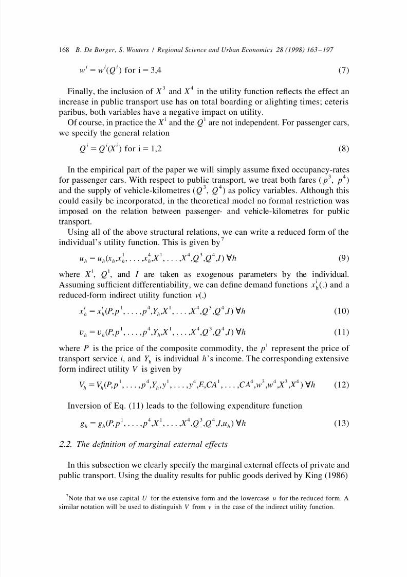
i i iw 5 w (Q ) for i 5 3,4 (7)
3 4Finally, the inclusion of X and X in the utility function reects the effect an
increase in public transport use has on total boarding or alighting times; ceterisparibus, both variables have a negative impact on utility.
i iOf course, in practice the X and the Q are not independent. For passenger cars,we specify the general relation
i i iQ 5 Q ( X ) for i 5 1,2 (8)
In the empirical part of the paper we will simply assume xed occupancy-rates3 4for passenger cars. With respect to public transport, we treat both fares ( p , p )
3 4and the supply of vehicle-kilometres ( Q , Q ) as policy variables. Although this
could easily be incorporated, in the theoretical model no formal restriction wasimposed on the relation between passenger- and vehicle-kilometres for publictransport.
Using all of the above structural relations, we can write a reduced form of the7individual’s utility function. This is given by
1 4 1 4 3 4u 5 u ( x , x , . . . , x , X , . . . , X ,Q ,Q , I ) ; h (9)h h h h h
i iwhere X , Q , and I are taken as exogenous parameters by the individual.iAssuming sufcient differentiability, we can dene demand functions x (.) and ah
reduced-form indirect utility function v(.)i i 1 4 1 4 3 4 x 5 x (P, p , . . . , p ,Y , X , . . . , X ,Q ,Q , I ) ; h (10)h h h
1 4 1 4 3 4v 5 v (P, p , . . . , p ,Y , X , . . . , X ,Q ,Q , I ) ; h (11)h h h
iwhere P is the price of the composite commodity, the p represent the price of transport service i, and Y is individual h’s income. The corresponding extensiveh
form indirect utility V is given by1 4 1 4 1 4 3 4 3 4V 5 V (P, p , . . . , p ,Y , y , . . . , y , E ,CA , . . . ,CA ,w ,w , X , X ) ; h (12)h h h
Inversion of Eq. (11) leads to the following expenditure function1 4 1 4 3 4g 5 g (P, p , . . . , p , X , . . . , X ,Q ,Q , I ,u ) ; h (13)h h h
2.2. The denition of marginal external effects
In this subsection we clearly specify the marginal external effects of private andpublic transport. Using the duality results for public goods derived by King (1986)
7Note that we use capital U for the extensive form and the lowercase u for the reduced form. Asimilar notation will be used to distinguish V from v in the case of the indirect utility function.
8/7/2019 Transport Ex Tern Ali Ties and Optimal Pricing and Supply
http://slidepdf.com/reader/full/transport-ex-tern-ali-ties-and-optimal-pricing-and-supply 7/35
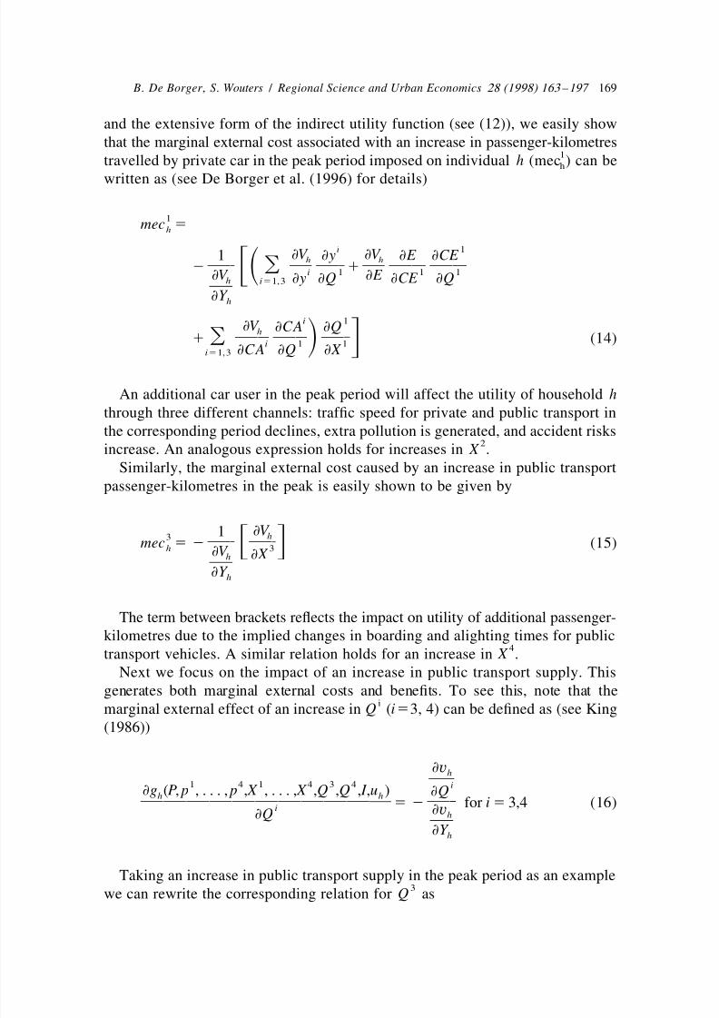
B. De Borger , S. Wouters / Regional Science and Urban Economics 28 (1998) 163 –197 169
and the extensive form of the indirect utility function (see (12)), we easily showthat the marginal external cost associated with an increase in passenger-kilometres
1travelled by private car in the peak period imposed on individual h (mec ) can beh
written as (see De Borger et al. (1996) for details)
1mec 5h
i 1≠V ≠V 1 ≠ y ≠ E ≠CE h h] ] ] ] ] ] ] ] ] ]2 O 1FS i 1 1 1≠V ≠ E ≠ y ≠Q ≠CE ≠Qh i 5 1,3]≠Y h
i 1≠V ≠CA ≠Qh] ] ] ] ] ]1 O (14)
D Gi 1 1≠
CA≠
Q≠ X i
5
1,3
An additional car user in the peak period will affect the utility of household hthrough three different channels: trafc speed for private and public transport inthe corresponding period declines, extra pollution is generated, and accident risks
2increase. An analogous expression holds for increases in X .Similarly, the marginal external cost caused by an increase in public transport
passenger-kilometres in the peak is easily shown to be given by
≠V 1 h3 ] ] ] ]mec 5 2 (15)F Gh 3≠V ≠ X h]≠Y h
The term between brackets reects the impact on utility of additional passenger-kilometres due to the implied changes in boarding and alighting times for public
4transport vehicles. A similar relation holds for an increase in X .Next we focus on the impact of an increase in public transport supply. This
generates both marginal external costs and benets. To see this, note that thei
marginal external effect of an increase in Q (i 5 3, 4) can be dened as (see King(1986))
≠ v h]1 4 1 4 3 4 i≠g (P, p , . . . , p , X , . . . , X ,Q ,Q , I ,u ) ≠Qh h]]]]]]]]]] ] ] ]5 2 for i 5 3,4 (16)i ≠ v h≠Q ]
≠Y h
Taking an increase in public transport supply in the peak period as an example3we can rewrite the corresponding relation for Q as

8/7/2019 Transport Ex Tern Ali Ties and Optimal Pricing and Supply
http://slidepdf.com/reader/full/transport-ex-tern-ali-ties-and-optimal-pricing-and-supply 8/35
170 B. De Borger , S. Wouters / Regional Science and Urban Economics 28 (1998) 163 –197
≠ gh] ] 53≠Q
i 3 i≠V ≠V ≠V 1 ≠ y ≠ E ≠CE ≠CAh h h] ] ] ] ] ] ] ] ] ] ] ] ] ]2 O 1 1 OF i 3 3 3 i 3≠V ≠ E ≠ y ≠ Q ≠CE ≠Q ≠CA ≠Qh i 5 1,3 i 5 1,3]≠Y h
3≠V ≠wh] ] ] ]1 (17)G3 3≠w ≠Q
This result clearly identies the different costs and benets. The rst three termsbetween brackets capture external costs: more peak-period supply contributes tocongestion by lowering travel speed, it generates extra pollution, and it increasesthe risk of accidents. The fourth term reects the benet of increased supply, viz.the decrease in waiting time for public transport passengers.
4A similar relation holds for Q . Finally, investment in infrastructure affectstravel speeds. Indeed, the external effect of extra infrastructural capacity is givenby
4 i≠g ≠V 1 ≠ yh h] ] ] ] ]5 2 O (18)F Gi≠ I ≠V ≠ I ≠ yh i 5 1]≠Y h
2.3. Organisation of the transport sector
It is assumed that both public transport and road infrastructure is provided bythe government. Total costs of road infrastructure are denoted C ( I ). Total costs of I
public transport consist of variable operating costs, capacity costs associated withrolling stock, and xed costs FC .
The capacity cost of rolling stock is generally specied as a function of thenumber of public transport vehicles B, C ( B). Variable operating costs of privateB
and public transport are given by
i i iC 5 C (Q ) for i 5 1,2 (19)
i i i iC 5 C (Q , X ) for i 5 3,4 (20)
iThe supply of vehicle-kilometres by public transport ( Q , i 5 3, 4) is constrainedby the number of available public transport vehicles B. Following Viton (1983),explicit capacity restrictions are imposed. Specically, the following inequalitiesshould be satised
i iQ # k B for i 5 3,4 (21)

8/7/2019 Transport Ex Tern Ali Ties and Optimal Pricing and Supply
http://slidepdf.com/reader/full/transport-ex-tern-ali-ties-and-optimal-pricing-and-supply 9/35
B. De Borger , S. Wouters / Regional Science and Urban Economics 28 (1998) 163 –197 171
iwhere the k may reect operating conditions (e.g. commercial speed), mainte-8nance policies etc.
2.4. Formulation of the optimisation problem
Two cases can be distinguished. Firstly, if there is no budget restriction imposedon the public transport rm, the model searches for optimal prices, optimal supplyof public transport, optimal number of buses, and optimal road infrastructure so asto solve the following problem:
MAX W [v , . . . ,v , . . . ,v ]1 h H 1 4 3 4 p , . . . , p ,Q ,Q , I , B
4i i i1 (1 1 l ) O ( p X 2 C ) 2 C ( B) 2 C ( I ) 2 FC F G B I
i 5 1(22)
k k s.t. Q # k B for k 5 3,4 ( m )k
1 2 3 4 p $ 0, p $ 0, p $ 0, p $ 0,3 4Q $ 0, Q $ 0, I $ 0, B $ 0
where W (.) is the relevant social welfare function, the v are given by (11), thehi 1 2 3 4 3 4aggregate demand functions X (P, p , p , p , p , Y , Q , Q , I ) are obtained byh
isumming the individual demands (10) over all h and solving for the X , and (11 l )is the marginal cost of public funds. In other words, we assume the governmentmaximises an objective function consisting of social welfare dened overindividual utilities plus government net revenues, evaluated at the marginal cost of public funds. Allowing for a marginal cost of public funds (1 1 l ) larger than onehas been suggested to account for existing distortions in the economy (e.g. due tothe impossibility of lump-sum taxation) in a partial equilibrium model (Laffontand Tirole, 1990).
Secondly, if the public transport authority does face a budget constraint, we addthe restriction
4 4i i iO C 1 C ( B) 1 FC # O p X 1 D (23) B
i 5 3 i 5 3
to the above optimisation problem, where D is the maximum allowed decit.
8 iIn the theoretical derivations it is assumed for simplicity that the k are exogenously given. Theempirical application on the other hand explicitly captures the dependency of these parameters onaverage speed, see below.

8/7/2019 Transport Ex Tern Ali Ties and Optimal Pricing and Supply
http://slidepdf.com/reader/full/transport-ex-tern-ali-ties-and-optimal-pricing-and-supply 10/35
172 B. De Borger , S. Wouters / Regional Science and Urban Economics 28 (1998) 163 –197
3. Optimal pricing rules and supply decisions
In this section we present optimal pricing and supply rules derived from the
formulated model. Note, however, that the presence of xed costs and externalitiesimplies non-convexities. It is well known that in this case the rst-order conditionsmay be insufcient and that corner solutions could be optimal (Guesnerie, 1980;
¨Bos, 1985). We restrict ourselves to a discussion of non-corner solutions.
3.1. No formal budget constraint
Using Roy’s identity, the duality results of King (1986), and dening s as theh
marginal social utility of income, it is easy to show that the rst-order conditionswith respect to prices can be summarized as follows
1 1≠C ≠Q1 2 3 4 1 1 1] ] ] ]h h h h S 1 l 2 (1 1 l ) p X S D1 1 1 1 1 1 ≠Q ≠ X
2 2≠C ≠Q1 2 3 4 2 2 2 ] ] ] ]h h h h S 1 l 2 (1 1 l ) p X S D2 2 2 2 2 2≠Q ≠ X 3 5
3 ≠C 1 2 3 4 3 3 3] ]h h h h S 1 l 2 (1 1 l ) p X
S D3 3 3 3 3
≠ X 4≠C 1 2 3 4 4 4 4] ]h h h h S 1 l 2 (1 1 l ) p X S D4 4 4 4 4 ≠ X 1 xh 1 1]O s 2 1 2 l p X S Dh 1 X h
2 xh 2 2 ]O s 2 1 2 l p X S Dh 2 X h2 (24)
3
xh 3 3]O s 2 1 2 l p X S Dh 3 X h 4 xh 4 4]O s 2 1 2 l p X S Dh 4 X h
iwhere h is the elasticity of demand for transport service i with respect to the price jiof service j, and S is the marginal social cost associated with an additional unit of
i X . It is dened as

8/7/2019 Transport Ex Tern Ali Ties and Optimal Pricing and Supply
http://slidepdf.com/reader/full/transport-ex-tern-ali-ties-and-optimal-pricing-and-supply 11/35
B. De Borger , S. Wouters / Regional Science and Urban Economics 28 (1998) 163 –197 173
i i≠C ≠Qi i ] ]S 5 O s mec 1 for i 5 1,2h h i i≠Q ≠ X h
(25)i
≠C i i ]S 5 O s mec 1 for i 5 3,4h h i≠ X h
Interestingly, the conditions for an optimal pricing structure are identical tothose derived in the case of a passive adaptation of public transport supply andxed infrastructure (De Borger et al., 1996). In other words, the availability of additional policy instruments does not affect the optimal pricing structure(although it may have a large impact on optimal price levels, see below).
The above results conrm the well-known fact that, if distortionary taxation is
assumed (i.e. l . 0), optimal pricing decisions depend in a complex way on theshadow cost of public funds, on all own and cross-elasticities, and on thedistributional characteristics of the different transport services. As usual, moreinsight can be obtained if one is willing to ignore distributional issues and assume
izero cross-elasticities of demand (i.e. assume h 5 0 except for i 5 j). Under those j
conditions the optimal pricing rules reduce to
i i1 l ≠C ≠Qi i] ] ] ] ] ] p 2 S 2i i1 1 l 1 1 l ≠Q ≠ X l 1]]]]]]]] ] ] ] ]5 2 for i 5 1,2 (26)
i i1 1 l p h i
i1 l ≠C i i] ] ] ] ] p 2 S 2i1 1 l 1 1 l l 1≠ X ]]]]]]] ] ] ] ]5 2 for i 5 3,4 (27)i i1 1 l p h i
These expressions show that optimal pricing requires a mark-up of price over aweighted average of marginal private and social cost; the mark-up is inversely
9
proportional to the price elasticity of demand. These ndings are consistent with,e.g. Sandmo (1975), and Oum and Thretheway (1988).Next consider the optimality conditions with respect to public transport supply
of vehicle-kilometres and with respect to infrastructure. They can be written as
9Alternatively, these relations imply a mark-up of price over private cost plus a fraction of externalcost. The mark-up is not over the full external cost. The reason is that an increase in price overmarginal private cost generates revenues for the transport sector while at the same time reducing thelevel of external effects.
8/7/2019 Transport Ex Tern Ali Ties and Optimal Pricing and Supply
http://slidepdf.com/reader/full/transport-ex-tern-ali-ties-and-optimal-pricing-and-supply 12/35
174 B. De Borger , S. Wouters / Regional Science and Urban Economics 28 (1998) 163 –197
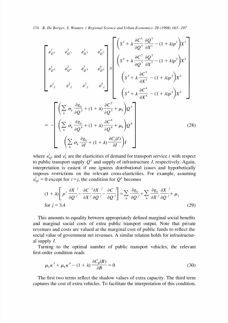
1 1≠C ≠Q1 1 1] ] ] ]S 1 l 2 (1 1 l ) p X S D1 1 ≠Q ≠ X 1 2 3 4´ ´ ´ ´ 3 3 3 3Q Q Q Q
2 2≠C ≠Q 2 2 2 ] ] ] ]S 1 l 2 (1 1 l ) p X S D2 2≠Q ≠ X 1 2 3 4 3´ ´ ´ ´ 4 4 4 4Q Q Q Q 3 ≠C 3 3 3] ]S 1 l 2 (1 1 l ) p X S D3≠ X 1 2 3 4 ´ ´ ´ ´ I I I I 4 ≠C 4 4 4] ]S 1 l 2 (1 1 l ) p X S D4 ≠ X
3≠g ≠C h 3] ] ] ]O s 1 (1 1 l ) 1 m Q
S Dh 3 3 3
≠ Q ≠Qh
4≠g ≠C h 45 2 ] ] ] ] (28)O s 1 (1 1 l ) 1 m QS Dh 4 4 4≠ Q ≠Qh ≠g ≠C ( I )h I ] ] ]O s 1 (1 1 l ) I S Dh ≠ I ≠ I
h
i iwhere ´ and ´ are the elasticities of demand for transport service i with respect jQ I jto public transport supply Q and supply of infrastructure I , respectively. Again,
interpretation is easiest if one ignores distributional issues and hypotheticallyimposes restrictions on the relevant cross-elasticities. For example, assumingi j´ 5 0 except for i 5 j, the condition for Q becomes jQ
j j j j j≠g ≠g≠ X ≠C ≠ X ≠C ≠ X h h j ] ] ] ] ] ] ] ] ] ] ] ] ](1 1 l ) p 2 2 5 O 1 O 1 mF G j j j j j j j j≠ Q ≠ X ≠Q ≠ Q ≠Q ≠ X ≠ Qh h
for j 5 3,4 (29)
This amounts to equality between appropriately dened marginal social benetsand marginal social costs of extra public transport output. Note that privaterevenues and costs are valued at the marginal cost of public funds to reect thesocial value of government net revenues. A similar relation holds for infrastructur-al supply I .
Turning to the optimal number of public transport vehicles, the relevantrst-order condition reads
≠C ( B) B3 4 ] ]m k 1 m k 2 (1 1 l ) 5 0 (30)3 4 ≠ B
The rst two terms reect the shadow values of extra capacity. The third termcaptures the cost of extra vehicles. To facilitate the interpretation of this condition,

8/7/2019 Transport Ex Tern Ali Ties and Optimal Pricing and Supply
http://slidepdf.com/reader/full/transport-ex-tern-ali-ties-and-optimal-pricing-and-supply 13/35
B. De Borger , S. Wouters / Regional Science and Urban Economics 28 (1998) 163 –197 175
suppose that the capacity restriction is binding in the peak period but not in the off peak so that m . 0 and m 5 0. Then (30) suggests that the social value of extra3 4
capacity should equal the extra costs, valued at one plus the shadow cost of public
funds.Finally, the capacity restrictions imply
j jk B 2 Q $ 0 for j 5 3,4 (31)
j jm [k B 2 Q ] 5 0 for j 5 3,4 (32) j
m $ 0, m $ 0 (33)3 4
It is easily shown that at the optimum at least one of the capacity restrictionswill be binding. To see this, consider Eq. (30) and note that the marginal cost of extra vehicles is always positive.
Finally, note that the interpretation of the optimality conditions can be furthersimplied if the government can use rst-best instruments. This amounts toassuming l 5 0 and ignoring redistributional concerns. In that case we obtain thewell-known rst-best rules:
3≠g ≠C hi i ] ] ] ]S 5 p ; i, O 1 1 m 5 0,3 3 3≠Q ≠Qh
(34)4≠g ≠g ≠ C ( I )≠C h h I ] ] ] ] ] ] ]O 1 1 m 5 0 and O 1 5 04 4 4 ≠ I ≠ I ≠Q ≠ Qh h
The optimum combines marginal social cost pricing with public transport supply
levels such that the marginal social cost of extra vehicle-kilometres, including theshadow price of the induced capacity expansion, equals marginal social benet.Similarly, levels of infrastructure are optimal when marginal costs equal marginalbenets.
3.2. Imposing a budget constraint on the public transport sector
The rst-order conditions describing optimal prices and optimal supply levelswhen budget restriction (23) is imposed on the public transport sector can berewritten as:

8/7/2019 Transport Ex Tern Ali Ties and Optimal Pricing and Supply
http://slidepdf.com/reader/full/transport-ex-tern-ali-ties-and-optimal-pricing-and-supply 14/35
176 B. De Borger , S. Wouters / Regional Science and Urban Economics 28 (1998) 163 –197
1 1≠C ≠Q1 2 3 4 1 1 1] ] ] ]h h h h S 1 l 2 (1 1 l ) p X S D1 1 1 1 1 1 ≠ Q ≠ X
2 2≠C ≠Q1 2 3 4 2 2 2 ] ] ] ]h h h h S 1 l 2 (1 1 l ) p X S D2 2 2 2 2 2≠ Q ≠ X
33
≠ C 1 2 3 4 3 3 3] ]h h h h S 1 ( l 1 f ) 2 (1 1 l 1 f ) p X S D3 3 3 3 3≠ X 4≠ C 1 2 3 4 4 4 4] ]h h h h S 1 ( l 1 f ) 2 (1 1 l 1 f ) p X S D4 4 4 4 4 ≠ X
1 xh 1 1]O s 2 1 2 l p X
S Dh 1
X h
2 xh 2 2 ]O s 2 1 2 l p X S Dh 2 X h5 2 (35)
3 xh 3 3]O s 2 1 2 l 2 f p X S Dh 3 X h
4 xh 4 4]O s 2 1 2 l 2 f p X S Dh 4 X h
1 1≠C ≠Q1 1 1] ] ] ]S 1 l 2 (1 1 l ) p X S D1 1 ≠ Q ≠ X 1 2 3 4´ ´ ´ ´ 3 3 3 3Q Q Q Q
2 2≠C ≠Q 2 2 2 ] ] ] ]S 1 l 2 (1 1 l ) p X S D2 2≠ Q ≠ X 1 2 3 4 3´ ´ ´ ´ 4 4 4 4Q Q Q Q 3 ≠C 3 3 3] ]S 1 ( l 1 f ) 2 (1 1 l 1 f ) p X S D3≠ X 1 2 3 4 ´ ´ ´ ´ I I I I
4
≠C 4 4 4] ]S 1 ( l 1 f ) 2 (1 1 l 1 f ) p X S D4 ≠ X
3≠g ≠ C h 3] ] ] ]O s 1 (1 1 l 1 f ) 1 m QS Dh 3 3 3≠ Q ≠Qh 4≠g ≠ C h 45 2 ] ] ] ] (36)O s 1 (1 1 l 1 f ) 1 m QS Dh 4 4 4≠ Q ≠Qh
≠ g ≠C ( I )h I ] ] ]O s 1 (1 1 l ) I
S Dh
≠ I ≠ I h

8/7/2019 Transport Ex Tern Ali Ties and Optimal Pricing and Supply
http://slidepdf.com/reader/full/transport-ex-tern-ali-ties-and-optimal-pricing-and-supply 15/35
B. De Borger , S. Wouters / Regional Science and Urban Economics 28 (1998) 163 –197 177
≠ C ( B) B3 4 ] ]m k 1 m k 2 (1 1 l 1 f ) 5 0 (37)3 4 ≠ B
j jk B 2 Q $ 0 for j 5 3,4 (38)
j jm [k B 2 Q ] 5 0 for j 5 3,4 (39) j
4 4i i iO p X 1 D 2 O C 2 C ( B) 2 FC $ 0 (40) B
i 5 3 i 5 3
4 4i i i
f O p X 1 D 2 O C 2 C ( B) 2 FC 5 0 (41)F G Bi 5 3 i 5 3
where f represents the multiplier associated with the budget restriction.Again, the results are much simplied if the government can use rst-best
redistributive taxation instruments (all s equal 1 and l 5 0) and cross-elasticitiesh
are restricted to zero. We nd under those circumstances
i i p 5 S for i 5 1,2 (42)
i1 f ≠ C i i] ] ] ] ] p 2 S 2i1 1 f 1 1 f f 1≠ X ]]]]]]] ] ] ] ]5 2 for i 5 3,4 (43)i i1 1 f p h i
Interestingly, note that marginal social cost pricing is optimal for private cartransport, but not for public transport. Zero cross-price elasticities imply that thereis no way car prices can be instrumental in generating modal shifts that might helpto satisfy the budgetary restriction. Consequently, there is no reason to deviatefrom social cost pricing for private car transport. However, for public transport a
mark-up over a weighted average of private and social cost should be charged thatis inversely proportional to the price elasticity of demand. Note that for publictransport the resulting pricing structure is essentially the same as the one obtainedin the case without budget restriction but where the marginal cost of fundsexceeded one. Optimal rules for public transport supply are also analogous; wend
j j j j j≠g ≠ g≠ X ≠C ≠ X ≠ C ≠ X h h j ] ] ] ] ] ] ] ] ] ] ] ] ](1 1 f ) p 2 2 5 O 1 O 1 mF G j j j j j j j j≠Q ≠ X ≠Q ≠Q ≠Q ≠ X ≠Qh h
for j 5 3,4 (44)
8/7/2019 Transport Ex Tern Ali Ties and Optimal Pricing and Supply
http://slidepdf.com/reader/full/transport-ex-tern-ali-ties-and-optimal-pricing-and-supply 16/35
178 B. De Borger , S. Wouters / Regional Science and Urban Economics 28 (1998) 163 –197
4. Implementation of the model
In what follows, we apply a simplied version of the model presented in the
theoretical section. Specically, we look for optimal transport prices and optimalsupply using Belgian data on urban transport. Due to current restrictions on dataavailability, the illustration is necessarily limited to a highly stylised application. Itis based on the use of aggregate data and therefore ignores distributionalconsiderations. Moreover, we assume throughout that the government can userst-best tax instruments.
In this section we provide information on the specication of the demand andsupply sides of the simulation model, and briey review the construction or thesources of the necessary data. We consecutively deal with the specication of thedemand functions, the structure of marginal social costs of additional private andpublic transport, the marginal social effects of additional infrastructure, and theconstruction of the budget constraint.
4.1. Specication of the demand functions
The model has to be interpreted as reecting an ‘aggregate’ Belgian urban area,consisting of all Belgian cities offering public urban transport. For the twotransport modes considered in the application, viz. the private car and publictransport, a distinction is made between peak and off-peak periods. The peak
period is assumed to cover 5 h a day, the off-peak period covers the remaining 17h (see STRATEC, 1992).The aggregate demand functions for the different transport services are taken to
be loglinear functions of the transport service prices, of the supply levels of publictransport, of the level of road infrastructure and of average speed
4 4i i i j i j i i i X 5 a exp O h ln( p ) 1 O ´ ln(Q ) 1 ´ ln( I ) 1 t ln( y ) (45) jS D j Q I i
j 5 1 j 5 3
To calibrate these demand functions, information is needed on elasticity values
(h , ´ , t ) and on levels of all relevant variables ( X , p, Q, B, I , y) in the referencesituation. A discussion of the data used is in Appendix A.
4.2. Marginal social costs and benets associated with additional trafc
1 2 4.2.1. Marginal social costs associated with additional car use ( S and S )
We assumed throughout that the occupancy rate of private cars was constant at1.7 persons per vehicle. As a consequence, a direct relation exists between themarginal social costs of an additional car-kilometre and those of an extrapassenger-kilometre. They consist of marginal congestion costs, marginal en-vironmental costs, marginal accident costs, and marginal private money costs.

8/7/2019 Transport Ex Tern Ali Ties and Optimal Pricing and Supply
http://slidepdf.com/reader/full/transport-ex-tern-ali-ties-and-optimal-pricing-and-supply 17/35
B. De Borger , S. Wouters / Regional Science and Urban Economics 28 (1998) 163 –197 179
To calculate marginal congestion costs associated with additional car users wefollowed the procedure described in De Borger et al. (1996) (p. 40), with a slightcorrection to accommodate endogenous infrastructure. Appendix B has some
details. The methodology basically consists of two steps. Firstly, we determinemarginal congestion, i.e. the time loss suffered by road users due to an extrakilometre travelled by car. Use is made of a congestion function calibrated withBelgian data. This relation describes how the average time needed to drive 1 kmby car depends on the total hourly trafc volume, expressed in passenger car
10equivalent unit kilometres (PCUkm/h), and on the level of road infrastructure. Itis assumed that the ratio of the average speed of public transport vehicles relativeto car speed is constant at | 0.77, reecting the relative speeds in the currentsituation. This information allowed us to calculate marginal congestion. The resultwas then combined with information on trafc composition and on respectivevalues of in-vehicle time of car and public transport users to estimate the marginalexternal congestion costs.
Due to the limited data available, the marginal external costs other thancongestion are assumed to be independent of trafc levels. The methodology istaken from Mayeres (1993); it is briey reviewed in De Borger et al. (1996, see
11Appendix). Application yielded marginal external accident costs equal to 0.648912BF per passenger-kilometre in both periods. With respect to the marginal
environmental costs, we make an explicit distinction between marginal airpollution costs and marginal noise costs. The marginal air pollution costsassociated with a car passenger-kilometre were calculated to be 0.354 BF, whilethe marginal noise costs associated with car use were found to be negligible(Mayeres, 1993).
The marginal private money costs associated with an additional car-kilometreinclude expenses on fuel, tyres, oil and maintenance. The average variable private
13money costs, exclusive of taxes , were used as an approximation of the relevantmarginal costs. Based on Cuijpers (1992), Zierock et al. (1989) and NIS (1988),
10 1 passenger car (PC) 5 1 passenger car equivalent unit (PCU), and 1 public transport vehicle
(PTV) 5 2 passenger car equivalent units.11 Note that the external cost gures used here differ from those used previously for both marginalaccident costs and marginal noise costs related to public transport use. See below for details.
12 Note that this gure is somewhat lower than the one used in De Borger et al. (1996). The reason isthat, as suggested by Jones-Lee (1990), we included in the earlier paper an allowance for the pain, grief and suffering experienced by relatives and friends as a component of marginal external accident costs.However, previous readers as well as Newbery (1988) have argued against this procedure, because it islikely that these costs are not external. Since they are imposed on friends and relatives they areprobably taken into account when drivers make their travel decisions. In the current paper we followedthis line of reasoning and did not include these costs as part of the marginal external accident costs.
13 These marginal private money costs can be interpreted as the ‘producer’ price. The differencebetween the optimal price (to be determined) and this producer price is the optimal tax to be levied onthe corresponding transport service.

8/7/2019 Transport Ex Tern Ali Ties and Optimal Pricing and Supply
http://slidepdf.com/reader/full/transport-ex-tern-ali-ties-and-optimal-pricing-and-supply 18/35
180 B. De Borger , S. Wouters / Regional Science and Urban Economics 28 (1998) 163 –197
14the average variable private money costs were estimated at 2.5525 BF pervehicle-kilometre or 1.5014 BF per passenger-kilometre. Note that these costswere assumed not to depend on trafc levels. In other words, the non-zero but
empirically small effect of trafc levels on energy consumption was ignored.
4.2.2. Marginal social costs and benets associated with additional publictransport
When discussing the marginal social costs and benets associated with extrapublic transport it is useful to distinguish between supply and demand effects. Theformer consider the impact of extra supply at a given level of demand forpassenger-kilometres. They include the extra monetary expenditures (on personnel,energy, materials, and reparations), marginal external costs (more congestion, moreenvironmental pollution and more accident costs), and external benets (a decreasein waiting time for the public transport passengers). In Section 4.2.2.1 we reporthow they were determined. Demand effects on the other hand look at extra costsassociated with an increase in the number of passenger-kilometres at a givensupply of vehicle-kilometres. Following Mohring (1972) and Viton (1983), it isassumed that an additional public transport passenger causes no additionalcongestion, environmental or accident costs. As a consequence, the relevant costssimply consist of marginal boarding and alighting time costs and marginal privatemoney costs. The procedure to calculate these costs is discussed in Section 4.2.2.2.
4.2.2.1. Marginal costs and benets associated with additional public transport supply
The marginal private money costs of public transport supply were approximatedby the average variable money costs, consisting of expenditures on drivers, energy(insofar as related to rolling stock), materials and reparations.
As previously suggested, the marginal external effects associated with additionalsupply of vehicle-kilometres by the public transport mode include congestion,environmental, and accident costs, as well as marginal reductions in waiting times.With the exception of the last component the procedure used to calculate therelevant external costs is similar to that used for private cars. Specically, to
calculate the marginal congestion costs associated with additional public transportvehicle-kilometres we rst determine the time loss suffered by road users, and nextestimate the monetary valuation of this loss. Again, all marginal external costsother than congestion costs are assumed to be constant. Marginal external airpollution costs associated with an additional bus-kilometre are estimated to be2.346 BF. Contrary to the situation for private car use, marginal external noisecosts were found not to be negligible for public buses. They were calculated usingan updated version of the procedure described in Boniver (1993) and amounted to
14 The variable private money costs are weighted by the proportion of total vehicle-kilometrestravelled with gasoline, diesel and LPG cars.

8/7/2019 Transport Ex Tern Ali Ties and Optimal Pricing and Supply
http://slidepdf.com/reader/full/transport-ex-tern-ali-ties-and-optimal-pricing-and-supply 19/35
B. De Borger , S. Wouters / Regional Science and Urban Economics 28 (1998) 163 –197 181
150.55 BF in the peak period and 1.88 BF in the off-peak period. Finally, themarginal external accident costs equal 2.5188 BF in both periods.
The marginal external benets associated with additional public transport
vehicle-kilometres equal the monetary value of the decrease in waiting time for allpublic transport passengers. To calculate the monetary value, we combine thedecrease in waiting time with the number of transit passengers and with theirvalues of waiting time.
We assume the average waiting time for a public transport vehicle (WT) to be16proportional to the inverse of frequency
1i ] ]WT ~iFreq
An indicator of frequency is obtained by dividing the number of public transportivehicle-kilometres during the period considered ( Q ) by the public transportnetwork length ( NL),
iQi ]Freq 5 NL
Using available information on network length, assumed constant at NL 5
1595.3 km, we found the inverse of frequency, i.e. the average headway, to be7.18 min in the peak and 12.57 min in the off-peak.
Instead of strictly applying the rule of thumb ‘wait equals half the headway’(Viton, 1983) we started from the observation that ‘the greater the headway of theservice, the bigger the proportion of passengers who will arrive to catch aparticular trip — above about 15 min headway, this probably applies to mostpassengers’ (Nash, 1982). We assumed that commuters and students heading forschool know the public transport timetable, and that, on average, they wait onethird of the headway. Other passengers are assumed to have somewhat lessinformation on the time schedule of public transport; they have an average waitingtime of half the headway. Based on these assumptions, and using data on therelative importance of trip motives, we found the proportionality factors to be 0.35
for the peak and 0.41 for the off-peak period. This implies that the average waitingtime is 2.51 min in the peak and 5.15 min in the off-peak.The monetary valuation of the decrease in waiting time due to an additional
public transport vehicle-kilometre can be found by differentiating the average
15 These gures are quite a bit lower than those used earlier (De Borger et al., 1996) for two reasons.One is the use of more recent information in several updated versions of Boniver (1993). The secondrelates to the recent correction of an error in the initial calculations reported there.
16 This is quite a common procedure in the literature; see, e.g. Mohring (1972), Jansson (1984), VanDeVoorde (1981). Some authors (e.g. Dodgson and Topham, 1987) have suggested other specications,however.

8/7/2019 Transport Ex Tern Ali Ties and Optimal Pricing and Supply
http://slidepdf.com/reader/full/transport-ex-tern-ali-ties-and-optimal-pricing-and-supply 20/35
182 B. De Borger , S. Wouters / Regional Science and Urban Economics 28 (1998) 163 –197
waiting time function with respect to Q and multiplying the result with the numberof public transport passengers and their values of waiting time. Using theobservation that the average distance travelled by public transport is 4 km
i
(Boniver, 1992), so that X /4 (i 5 3, 4) corresponds to the number of publictransport passengers in period i, the marginal external waiting time benet( MEWB ) associated with extra public transport supply can be written asi
i i i≠WT X hoursi] ] ] ] ] MEWB 5 2 VOWT for i 5 3,4S Di i 4 period ≠Qi iwhere VOWT is the value of waiting time and (hours /period) equals 5 and 17 for
the peak and off-peak, respectively. Values of waiting time for public transportusers were derived from Visser and van der Mede (1988), Bradley (1990) and
Gunn (1991). We used 218 BF per peak hour and 208 BF per off-peak hour.
4.2.2.2. Marginal social costs associated with additional public transport pas -3 4
senger -km ( S and S ) As previously suggested the marginal social costs associated with additional
public transport passenger-kilometres simply consist of marginal boarding andalighting time costs and marginal private money costs for the transport companies.
iMarginal boarding and alighting time costs ( MBATC ) associated with anadditional public transport passenger can be written
i
X i i] MBATC 5 MBAT ? ? IVT for i 5 3,4iQ
where MBAT is the marginal boarding/alighting time due to an extra passenger-ikilometre and IVT is the value of in-vehicle time.
The marginal boarding/alighting time for an additional passenger was taken tobe 2.5 s (Jansson, 1984; Glaister, 1985). Using an average distance travelled by apublic transport passenger of 4 km (Boniver, 1992), the marginal boarding/ alighting time for an additional passenger-kilometre equals 0.625 s. Of course, all
i ibus travellers — on average there are X / Q people aboard — experience this17
delay. Their value of in-vehicle time was calculated to be 151 BF per peak hourand 137 BF per hour in the off-peak period (Gunn, 1991). Using this informationyields the marginal boarding and alighting time costs associated with an additionalpublic transport passenger.
The private money costs for the transport companies caused by an additional
17 By boarding or alighting the passenger will cause some people further along the route to waitlonger. Other people will have to wait for a shorter time, since they would have had to wait for the nextbus if this one had not been delayed. Following Turvey and Mohring (1975), we assume that these twoeffects neutralise each other.

8/7/2019 Transport Ex Tern Ali Ties and Optimal Pricing and Supply
http://slidepdf.com/reader/full/transport-ex-tern-ali-ties-and-optimal-pricing-and-supply 21/35
B. De Borger , S. Wouters / Regional Science and Urban Economics 28 (1998) 163 –197 183
18passenger are estimated to be in the range of 0.35–1.1 BF. In view of an averagedistance travelled by a public transport passenger of 4 km, we used 0.2 BF as acrude estimate of the marginal private money cost.
4.3. Marginal effects of additional road infrastructure
Following Viton (1983), we assume that the location and length of the road isgiven, such that the decision variable I has to be interpreted as the number of lane-kilometres supplied. We estimated that in the reference year 1989 there were| 15 000 lane-kilometres in the relevant urban areas.
Additional road infrastructure involves costs and benets. Firstly, the averageconstruction, maintenance and expropriate costs were used as an approximation of the marginal infrastructure costs. These costs were determined at 6248 BF perlane-kilometre and per day. Secondly, when more lane-kilometres are available,trafc can move faster, resulting in a decreasing time needed to travel 1 km. The
Imonetary value of this time saving ( MB ) can be calculated as follows4 i≠ t I i i] MB 5 O ? X ? IVT ≠ I i 5 1
iwhere t is the relevant congestion function (see Appendix B).
4.4. The budget constraint
The budget constraint on the public transport sector implies that the sum of allvariable private costs of public transport, the capacity costs of rolling stock, andthe xed costs should be covered by public transport revenues plus a maximumallowed decit (or surplus). The necessary information was directly obtained fromthe transport companies’ annual reports.
5. Some simulation results for Belgium
In this section, we report some simulation results obtained using the non-linear19optimisation program GAMS/ MINOS (Brooke et al., 1992). We rst carefully
18 This cost information is based on interviews with representatives of the study department of thebus company. The marginal private money costs are the material costs associated with providingpassengers with tickets.
19 Of course, the model uses a large number of estimated parameters and data from a variety of sources. In order to test the sensitivity of the results with respect to the most important demand and costparameters a substantial number of additional simulations were carried out. Not surprisingly, we foundthe numerical results to be somewhat sensitive to the assumed own price elasticities, to variations in themarginal private cost of public transport, and to the initial level of infrastructure. However, thequalitative conclusions to be derived from these exercises were in no way affected.

8/7/2019 Transport Ex Tern Ali Ties and Optimal Pricing and Supply
http://slidepdf.com/reader/full/transport-ex-tern-ali-ties-and-optimal-pricing-and-supply 22/35
184 B. De Borger , S. Wouters / Regional Science and Urban Economics 28 (1998) 163 –197
discuss the results of the basic model, in which no budgetary restrictions areimposed; next we consider models with a budget constraint for the public transport
20sector. In describing the results three issues are of interest. Firstly, we want to
know to what extent the optimal values for the policy variables (prices, publictransport supply, level of road infrastructure), the corresponding trafc levels, andthe marginal social costs and average speeds differ from the values observed in theinitial situation. In other words, how large are the adjustments required toimplement the optimum. Secondly, we are interested to nd out what theimplications of optimal supply adjustments are for the resulting price structure.Comparison with the results obtained under the assumption of passive adaptationof supply and xed road capacity will prove useful here. Thirdly, we consider theeffects of optimal pricing and supply characteristics for the performance of thepublic bus operator in terms of occupance rates, budgetary decits, and overallproductivity.
5.1. Basic model : no budget constraint
In the absence of budgetary constraints and assuming that the government canuse rst-best instruments, optimal prices were shown to equal marginal socialcosts, and optimal supply levels were found to be such that the marginal socialcost of extra supply, including the shadow price of extra vehicles, equals themarginal social benet. Relevant simulation results for this case are given in Table1. For each variable, Table 1 contains the observed value in the reference situation,the optimal value, and the percentage change.
Firstly, consider the optimal prices of the basic model. For car transport, optimalprices turn out to be substantially higher than current price levels. Specically,internalisation of externalities yields car prices in the peak that are 86% abovecurrent prices, whereas off-peak prices have risen by 12% compared to referenceprices. Since, conditional on capacity and quantity of vehicle-kilometres supplied,extra passengers imply a relatively low marginal cost (i.e. consisting of marginalboarding and alighting time costs and the marginal costs associated with handlingtickets), the optimal prices for public transport combined with optimal supply
decisions are in both periods considerably below current prices. Public transportprices decrease by 61% in the peak, and by 84% in the off-peak period. Finally,note that optimal prices per passenger-kilometre are higher for private transportthan for public transport, unlike current prices.
Optimal supply of public transport in the peak period is 13% higher than the1989 supply level; for the off-peak period, the increase even amounts to 54%. Thereason for the substantial increase in off-peak public transport supply is due to the
20 i iNote that, in the simulations, we relax the assumption that k is constant. k is here dened suchithat the number of vehicle-kilometres supplied in the peak and off-peak period ( Q ) is bounded by the
distance B buses are able to travel during the relevant period.

8/7/2019 Transport Ex Tern Ali Ties and Optimal Pricing and Supply
http://slidepdf.com/reader/full/transport-ex-tern-ali-ties-and-optimal-pricing-and-supply 23/35
B. De Borger , S. Wouters / Regional Science and Urban Economics 28 (1998) 163 –197 185
Table 1Simulation results: optimal pricing and supply results
Initial Basic optimum without budget constraint
situationOptimal values % change
w.r.t. initialsituation
Prices (BF per passenger km)Car Peak 2.665 4.968 86.42%
Off-peak 2.665 2.986 12.05%Bus and tram Peak 3.460 1.345 2 61.13%
Off-peak 3.460 0.550 2 84.10%SupplyInfrastructure (lane km) 15 000 19 850 32.33%
Bus and tram (vehicle km a day) Peak 66 651 75 432 13.17%Off-peak 129 382 199 817 54.44%
Bus and tram (buses a day) 577 506
Marginal social costs of passenger km(BF per passenger km)Car Peak 11.635 4.968 2 57.30%
Off-peak 3.244 2.986 2 7.95%Bus and tram Peak 0.781 1.345 72.22%
Off-peak 0.415 0.550 32.53%
Marginal social effects of public transport vehicle km(BF per vehicle km)Marginal social costs Peak 85.175 55.100 2 35.31%
Off-peak 47.008 45.472 2 3.27%
Marginal social benets Peak 52.899 90.093 70.31%Off-peak 44.808 45.472 1.48%
Trafc ow(mio passenger km a day)Car Peak 47.313 40.968 2 13.41%
Off-peak 48.695 45.608 2 6.34%Total 96.008 86.576 2 9.82%
Bus and tram Peak 1.544 3.369 118.14%Off-peak 1.297 3.140 142.05%Total 2.842 6.509 129.06%
Total passenger km (mio a day) 98.849 93.085 2 5.83%Total vehicle km (mio a day) 56.671 51.202 2 9.65%
Average speed (km/h)Car Peak 30.000 38.735 29.12%
Off-peak 45.271 46.702 3.16%Bus and tram Peak 23.100 29.826 29.12%
Off-peak 34.859 35.961 3.16%
Surplus (BF a day)Transport sector as a whole 2 72.657 62 054 400 2 85 507.80%Private transport sector 17 994 400 85 727 100 376.41%Public transport sector 2 18 067 070 2 23 672 650 31.03%
Multipliers
Capacity constraint peak m 3 34.916Capacity constraint off-peak m 4 0Budget restriction f 0

8/7/2019 Transport Ex Tern Ali Ties and Optimal Pricing and Supply
http://slidepdf.com/reader/full/transport-ex-tern-ali-ties-and-optimal-pricing-and-supply 24/35
186 B. De Borger , S. Wouters / Regional Science and Urban Economics 28 (1998) 163 –197
observation that reductions in waiting time can be realised at very low extra costs.Since the capacity of vehicles is determined by transport needs in the peak periodthe marginal cost of extra vehicle-kilometres in the off-peak is small. The optimal
21
level of infrastructure is about 22% higher than the estimated current level.It is interesting to compare the implications of optimal supply adjustments for
the level and structure of optimal prices. To get some insight into this question wecompare the pricing results obtained under the assumption of xed infrastructureand passive adaptation of public transport supply (De Borger et al., 1996) with
22those of the current paper. Two conclusions emerge from this exercise. Firstly,allowing for the possibility of optimal adjustments in supply characteristics impliesthat optimal prices for car trafc are lower: assuming passive adaptation of supplyyielded price increases of 150% (compared to 86% in the current paper) and 30%(compared to 12%) for peak and off-peak car trafc, respectively. The reason forthis phenomenon is that the reduction in public transport prices combined withincreasing supply yields a shift from car to public transport. The shift to the left of the demand for car travel implies lower congestion, and therefore smaller optimalprice increases are necessary to cover marginal social costs. Secondly, withoptimal supply adjustments public transport prices are much lower as well. If theadditional supply instruments were not available public transport prices in the peak actually increased by some 22% in the peak period (compared to a 61% reductionin the current paper). There are two reasons for this nding. Firstly, optimal supplyadjustments allow a reduction in marginal social costs associated with publictransport. Secondly, calculation of the marginal social costs of extra vehiclekilometres differs substantially depending on the assumptions made with respect tothe supply of public transport. Assuming passive supply adjustments to demandvariations implies that the marginal social cost of an extra vehicle kilometre can bedirectly allocated to passengers. In the current model the marginal social cost of extra vehicle kilometres played a crucial role in determining optimal supply, andthe social cost of extra passenger kilometres were mainly limited to boarding andalighting time costs.
Returning to the results of the current model application, note that the optimalfare and supply structure causes 13% and 6% reductions in peak and off-peak car
23
trafc, respectively. The negative impact of the own price increases clearlydominate cross-price effects and the positive demand effect of the increase in
21 Sensitivity analysis suggested that the optimal level of infrastructure was not very sensitive to theassumed level in the reference situation.
22 Note that slightly different external cost gures were used in the current paper (see the discussionof accident and noise costs above). However, given the small share of these costs in the full marginalexternal cost of transport, which is mainly dominated by external congestion costs, a comparison of results of the current paper with those of the earlier analysis seems acceptable.
23 These effects are slightly smaller than in De Borger et al. (1996). The reason is that the expansionof infrastructure in the current model solution reduces congestion at given trafc volumes; therefore,some extra trafc is generated.

8/7/2019 Transport Ex Tern Ali Ties and Optimal Pricing and Supply
http://slidepdf.com/reader/full/transport-ex-tern-ali-ties-and-optimal-pricing-and-supply 25/35
B. De Borger , S. Wouters / Regional Science and Urban Economics 28 (1998) 163 –197 187
average speed. Not surprisingly, the percentage changes in public transport use aremuch more pronounced. We note an increase by 118% and 142% for the peak andthe off-peak period, respectively. These results are mainly induced by the
reduction in fares and the increase in public transport supply. Of course, theabsolute magnitude of the percentage changes should be interpreted in view of thesmall share of public transport in the reference situation. In 1989, the share of theprivate car was about 97%.
The ultimate result is a 6% decrease in the total number of passenger-kilometres. Total car trafc decreases by 10%, whereas public transport useincreases by 129%. The share of public transport rises from 3% to some 7%. Thisshift is consistent with expectations. Note that in this respect our results are not aspronounced as those in Viton (1983). He found extreme transit-favoring modalsplits (up to a 100% share of public transport in some simulations) when allpricing and investment decisions are made correctly.
In comparison with the initial situation, marginal social costs of car use havebeen reduced, whereas those associated with public transport use have beenincreased. For private car and public transport, the change in marginal social costsassociated with peak trafc is larger than the one associated with off-peak trafc.In both periods, the percentage change in marginal social costs is larger for thepublic transport mode than for the private mode. Note that the changes are actuallyquite substantial.
Implementation of the optimal pricing and supply structure has importantimplications for the performance of the public transport sector. Firstly, the increasein the number of passenger-kilometres travelled by public transport involves asubstantial increase in occupancy rates; in 1989 there were on average 23 peopleon a public transport vehicle in the peak and 10 in the off-peak, whereas in theoptimum there are on average 44 people aboard in the peak and 15 in the off-peak.In terms of the environmental impact it is interesting to note that the number of vehicle-kilometres travelled declines by 10%. Secondly, the reduction in conges-tion in the optimum and the increased use of public transport have a somewhatsurprising side-effect. Indeed, compared to the initial situation, the optimum yieldsa 12% decrease in the number of public transport vehicles B despite the increase in
public transport supply. Higher average speed (an increase of almost 30% in thepeak) allows public transport companies to provide more services with a somewhatsmaller eet. In this sense, productivity is clearly enhanced. Note, by the way, thatthe capacity constraint is binding in the peak period and non-binding in theoff-peak period, as was expected.
A third and important nding relates to the implications of pricing forgovernment revenues out of public and private transport. It is found that withoptimal prices and supply levels the decit of the public transport sector increasesby 31%. However, this is more than compensated by the increase in governmentrevenues due to heavier taxation of car use. Overall, the decit of the transportsector is transformed into a sizeable surplus.

8/7/2019 Transport Ex Tern Ali Ties and Optimal Pricing and Supply
http://slidepdf.com/reader/full/transport-ex-tern-ali-ties-and-optimal-pricing-and-supply 26/35
188 B. De Borger , S. Wouters / Regional Science and Urban Economics 28 (1998) 163 –197
T a b l e
2
S i m u
l a t i o n r e s u
l t s : i m p o s i n g a p u b
l i c t r a n s p o r t s e c t o r
b u d g e t r e s t r i c t i o n
B a s i c
O p t i m u m w i t h b u d g e t c o n s t r a i n t 1
O p t i m u m w i t h b u d g e t c o n s t r a i n t 2
O p t i m u m w i t h b u d g e t
c o n s t r a i n t 3
o p t i m u m
D 5
i n i t i a l d e c i t
D 5
9 0 % o f i n i t i a l d e c i t
D 5
7 0 % o f i n i t i a l d e c i t
O p t i m a l
O p t i m a l
% c h a n g e
O p t i m a l
% c h a n g e
O p t i m a l
% c h a n g e
v a l u e s
v a l u e s
w . r . t
b a s i c
v a l u e s
w . r . t .
b a s i c
v a l u e s
w . r . t .
b a s i c
o p t i m u m
o p t i m u m
o p t i m u m
P r i c e s ( B F p e r p a s s e n g e r k m )
C a r
P e a k
4 . 9 6 8
5 . 3 5 2
7 . 7 3 %
5 . 4 9 2
1 0 . 5 5 %
5 . 7 8 6
1 6 . 4 7 %
O f f - p e a k
2 . 9 8 6
3 . 0 4 1
1 . 8 4 %
3 . 0 5 9
2 . 4 4 %
3 . 0 9 5
3 . 6 5 %
B u s a n d t r a m
P e a k
1 . 3 4 5
2 . 7 5 4
1 0 4 . 7 6 %
3 . 0 9 8
1 3 0 . 3 3 %
3 . 6 1 2
1 6 8 . 5 5 %
O f f - p e a k
0 . 5 5 0
0 . 9 6 1
7 4 . 7 3 %
1 . 1 1 8
1 0 3 . 2 7 %
1 . 4 7 9
1 6 8 . 9 1 %
S u p p l y
I n f r a s t r u c t u r e ( l a n e k m )
1 9 8 5 0
1 9 8 5 8
0 . 0 4 %
1 9 8 3 6
2 0 . 0 7 %
1 9 7 8 1
2 0 . 3 5 %
B u s a n d t r a m
( v e h i c l e k m a d a y )
P e a k
7 5 4 3 2
1 1 1 7 1 4
4 8 . 1 0 %
1 2 7 8 7 3
6 9 . 5 2 %
1 6 3 0 2 9
1 1 6 . 1 3 %
O f f - p e a k
1 9 9 8 1 7
1 7 4 3 2 8
2 1 2 . 7 6 %
1 6 9 3 3 3
2 1 5 . 2 6 %
1 6 1 0 9 1
2 1 9 . 3 8 %
B u s a n d t r a m ( b u s e s a d a y )
5 0 6
7 4 8
4 7 . 7 9 %
8 5 5
6 8 . 9 8 %
1 0 8 7
1 1 4 . 9 3 %
M a r g i n a l s o c i a l c o s t s o f p a s s e n g e r
k m ( B F p e r p a s s e n g e r k m )
C a r
P e a k
4 . 9 6 8
4 . 9 7 5
0 . 1 4 %
4 . 9 7 8
0 . 2 0 %
4 . 9 8 6
0 . 3 6 %
O f f - p e a k
2 . 9 8 6
2 . 9 8 4
2 0 . 0 7 %
2 . 9 8 5
2 0 . 0 3 %
2 . 9 8 5
2 0 . 0 3 %
B u s a n d t r a m
P e a k
1 . 3 4 5
1 . 1 3 2
2 1 5 . 8 4 %
1 . 0 9 1
2 1 8 . 8 8 %
1 . 0 3 4
2 2 3 . 1 2 %
O f f - p e a k
0 . 5 5 0
0 . 5 2 0
2 5 . 4 5 %
0 . 5 1 0
2 7 . 2 7 %
0 . 4 9 0
2 1 0 . 9 1 %
M a r g i n a l s o c i a l e f f e c t s o f p u b l i c t r a n s p o r t v e h i c l e k m ( B F
p e r v e h i c l e k m )
M a r g i n a l s o c i a l c o s t s
P e a k
5 5 . 1 0 0
5 5 . 0 2 1
2 0 . 1 4 %
5 4 . 9 8 7
2 0 . 2 1 %
5 4 . 9 1 4
2 0 . 3 4 %
O f f - p e a k
4 5 . 4 7 2
4 5 . 4 7 0
2 0 . 0 0 %
4 5 . 4 7 3
0 . 0 0 %
4 5 . 4 8 1
0 . 0 2 %

8/7/2019 Transport Ex Tern Ali Ties and Optimal Pricing and Supply
http://slidepdf.com/reader/full/transport-ex-tern-ali-ties-and-optimal-pricing-and-supply 27/35
B. De Borger , S. Wouters / Regional Science and Urban Economics 28 (1998) 163 –197 189
M a r g i n a l s o c i a l b e n e t s
P e a k
9 0 . 0 9 3
4 9 . 7 8 9
2 4 4 . 7 4 %
4 1 . 6 2 8
2 5 3 . 7 9 %
3 0 . 6 3 9
2 6 5 . 9 9 %
O f f - p e a k
4 5 . 4 7 2
4 7 . 9 9 3
5 . 5 4 %
4 7 . 9 3 2
5 . 4 1 %
4 7 . 4 1 7
4 . 2 8 %
T r a f c o w ( m i o p a s s e n g e r k m a d a y )
C a r
P e a k
4 0 . 9 6 8
4 0 . 6 1 7
2 0 . 8 6 %
4 0 . 3 9 0
2 1 . 4 1 %
3 9 . 8 7 9
2 2 . 6 6 %
O f f - p e a k
4 5 . 6 0 8
4 5 . 8 1 4
0 . 4 5 %
4 5 . 8 5 1
0 . 5 3 %
4 5 . 9 0 2
0 . 6 4 %
T o t a l
8 6 . 5 7 6
8 6 . 4 3 0
2 0 . 1 7 %
8 6 . 2 4 1
2 0 . 3 9 %
8 5 . 7 8 0
2 0 . 9 2 %
B u s a n d t r a m
P e a k
3 . 3 6 9
4 . 0 8 4
2 1 . 2 1 %
4 . 4 7 4
3 2 . 7 8 %
5 . 3 5 2
5 8 . 8 5 %
O f f - p e a k
3 . 1 4 0
2 . 5 2 3
2 1 9 . 6 7 %
2 . 3 7 7
2 2 4 . 3 0 %
2 . 1 2 8
2 3 2 . 2 3 %
T o t a l
6 . 5 0 9
6 . 6 0 6
1 . 4 9 %
6 . 8 5 1
5 . 2 5 %
7 . 4 8 0
1 4 . 9 2 %
T o t a l p a s s e n g e r k m ( m i o a d a y )
9 3 . 0 8 5
9 3 . 0 3 7
2 0 . 0 5 %
9 3 . 0 9 1
0 . 0 1 %
9 3 . 2 6 1
0 . 1 9 %
T o t a l v e h i c l e
k m ( m i o a d a y )
5 1 . 2 0 2
5 1 . 1 2 7
2 0 . 1 5 %
5 1 . 0 2 7
2 0 . 3 4 %
5 0 . 7 8 3
2 0 . 8 2 %
A v e r a g e s p e e d ( k m / h )
C a r
P e a k
3 8 . 7 3 5
3 8 . 8 1 7
0 . 2 1 %
3 8 . 8 5 9
0 . 3 2 %
3 8 . 9 5 1
0 . 5 6 %
O f f - p e a k
4 6 . 7 0 2
4 6 . 6 9 5
2 0 . 0 1 %
4 6 . 6 9 0
2 0 . 0 3 %
4 6 . 6 7 8
2 0 . 0 5 %
B u s a n d t r a m
P e a k
2 9 . 8 2 6
2 9 . 8 8 9
0 . 2 1 %
2 9 . 9 2 1
0 . 3 2 %
2 9 . 9 9 2
0 . 5 6 %
O f f - p e a k
3 5 . 9 6 1
3 5 . 9 5 5
2 0 . 0 2 %
3 5 . 9 5 1
2 0 . 0 3 %
3 5 . 9 4 2
2 0 . 0 5 %
S u r p l u s ( B F a d a y )
T r a n s p o r t s e c t o r a s a w h o l e
6 2 0 5 4 4 0 0
8 4 7 9 4 9 0 0
3 6 . 6 5 %
9 2 4 1 6 7 0 0
4 8 . 9 3 %
1 0 7 7 9 1 0 0 0
7 3 . 7 0 %
P r i v a t e t r a n s p o r t s e c t o r
8 5 7 2 7 1 0 0
1 0 2 8 6 2 0 0 0
1 9 . 9 9 %
1 0 8 6 7 7 0 0 0
2 6 . 7 7 %
1 2 0 4 3 8 0 0 0
4 0 . 4 9 %
P u b l i c t r a n s p o r t s e c t o r
2 2 3 6 7 2 6 5 0
2 1 8 0 6 7 0 7 0
2 2 3 . 6 8 %
2 1 6 2 6 0 3 6 0
2 3 1 . 3 1 %
2 1 2 6 4 6 9 5 0
2 4 6 . 5 8 %
M u l t i p l i e r s
C a p a c i t y c o n s t r a i n t p e a k
m 3
3 4 . 9 1 6
3 8 . 6 2 6
3 8 . 9 7 2
3 9 . 3 1 5
C a p a c i t y c o n s t r a i n t o f f - p e a k
m 4
0
0
0
0
B u d g e t r e s t r i c t i o n
f
0
0 . 1 0 9
0 . 1 2
0 . 1 3 2

8/7/2019 Transport Ex Tern Ali Ties and Optimal Pricing and Supply
http://slidepdf.com/reader/full/transport-ex-tern-ali-ties-and-optimal-pricing-and-supply 28/35
190 B. De Borger , S. Wouters / Regional Science and Urban Economics 28 (1998) 163 –197
5.2. Introduction of a budget constraint on the public transport sector
The increased public transport decit at optimal prices may not be socially or
politically acceptable. We therefore also illustrate the impact of budgetaryconstraints on the public transport sector. Table 2 reports some results. The rstcolumn repeats the results of the basic optimum without budget constraint as abasis for comparison. The second column gives the results for the case where themaximum public transport decit allowed is the observed decit for 1989.Columns 3 and 4 report simulation results for more restrictive decit constraints;they refer to a 10% and a 30% reduction in the observed decit, respectively.
In order to remain within the observed 1989 budget all optimal prices have torise in comparison with the unconstrained optimum (see column 2). This is notsurprising, because the 1989 transport decit is substantially (some 24%) belowthe level at the unconstrained optimum. Public transport prices increase by 105%in the peak and 75% in the off-peak. The budget restriction on the public transportsector also makes car use more expensive. With non-zero cross price elasticities,the increasing public transport prices imply increasing congestion. To counteractthis negative effect optimal car prices rise as well, viz. by 8% in the peak and 2%in the off-peak.
Interestingly, imposition of a budget restriction implies a decrease in optimalpublic transport supply in the off-peak period, but an increase in peak-periodsupply as well as in the optimal number of public transport vehicles. Theseseemingly strange results can be explained as follows. First consider peak-periodsupply of vehicle-kilometres. Extra supply induces more people to use publictransport. However, as public transport prices exceed marginal social costs of extrapassenger-kilometres at the optimum (and therefore certainly marginal privatecosts), the extra revenues that are generated by far exceed the extra variableoperating costs associated with serving more passengers. This revenue increasemore than offsets the marginal private cost of extra supply of vehicle-kilometres(including the cost of extra capacity), resulting in an increase in prot for thepublic transport company. The requirement to cut the decit is therefore consistentwith both more peak public transport supply and an increase in the number of
public transport vehicles operated.Despite a higher capacity of available vehicles, supply in the off-peak perioddeclines due to more stringent budgetary restrictions. To understand this, note thatprice increases are much less pronounced than in the peak. As a consequence, therevenue increase generated by the extra demand for off-peak travel induced bymore off-peak supply is insufcient to cover the extra direct (associated with extrasupply) and indirect (associated with supply-induced extra passengers) operatingcosts. Therefore, the imposition of a budget constraint leads to a decrease in thenumber of off-peak vehicle-kilometres supplied.
Imposing a budget restriction affects the modal composition of transport ows,but, as can be seen in Table 2, total transport demand is hardly affected. Similarly,

8/7/2019 Transport Ex Tern Ali Ties and Optimal Pricing and Supply
http://slidepdf.com/reader/full/transport-ex-tern-ali-ties-and-optimal-pricing-and-supply 29/35
B. De Borger , S. Wouters / Regional Science and Urban Economics 28 (1998) 163 –197 191
the impact on average speed is also very small. Finally, the results do yield higheroccupancy rates for public transport vehicles: imposing the 1989 decit as arestriction implies average occupancy rates of 36 and 14 passengers in the peak
and off-peak periods, respectively.Columns 3 and 4 in Table 2 indicate that, as expected, more stringent budget
restrictions lead to even higher prices for all modes. Moreover, it results in anincrease in peak public transport supply, a decrease in off-peak public transportsupply, an increase in the number of buses used, and a decrease in the number of lane-kilometres available. Average speed of the different modes hardly changes.These trends imply small changes in private car use and more substantial changesin public transport use. However, the total number of passenger-kilometres andvehicle-kilometres travelled remains approximately constant.
A nal remark is in order. The exercises reported in this paper clearly suggestthat socially optimal pricing and supply decisions may require adjustments incurrent prices and public transport supply that are so large as to be politicallyunacceptable. However, the purpose of this paper was not to come up with animmediately applicable pricing structure. Its primary purpose was precisely toprovide information on the magnitude of the deviations of the current pricingstructure and public transport supply levels from their socially optimal levels,determined by taking all relevant externalities into account. The most desirablepath towards this social optimum was not explicitly studied in this paper.
6. Conclusions
In this paper, we analyzed the introduction of social cost considerations in thepricing of urban transport and in the determination of the optimal supply levels of both public transport and road infrastructure. The model was applied to studyoptimal transport prices and optimal supply levels using Belgian data. Due tolimitations on data availability the empirical analysis uses aggregate data andtherefore ignores distributional considerations. It does capture all relevant privateand external costs (associated with, e.g. congestion, air pollution, noise, accident
risks, and boarding and alighting times) as well as external benets associated withadditional public transport and road infrastructure.Ignoring distributional and budgetary considerations, optimal prices were found
to be well above the 1989 level for private transport (86% in the peak period and12% in the off-peak period). For public transport, the model yields optimal pricesthat are much lower than the 1989 fares (61% in the peak and 84% in theoff-peak). Optimal prices are higher in the peak than in the off-peak, and in bothperiods optimal transport prices are higher for private car use than for publictransport use. Optimal supply of public transport is substantially above the actualsupply level for the peak and off-peak period. Furthermore, there is a 32% increasein lane capacity of the road system. Interestingly, we found that explicitly
8/7/2019 Transport Ex Tern Ali Ties and Optimal Pricing and Supply
http://slidepdf.com/reader/full/transport-ex-tern-ali-ties-and-optimal-pricing-and-supply 30/35
192 B. De Borger , S. Wouters / Regional Science and Urban Economics 28 (1998) 163 –197
accounting for optimal supply adjustments reduce the price increases that arenecessary to balance prices and marginal social costs. When all prices and supplylevels are optimally determined, we further observe a 6% decrease in the number
of passenger-kilometres travelled. The number of vehicle-kilometres is reduced by10%. The increase in lane capacity and the decrease of vehicle-kilometres travelledinvolve an increase in average speed for both modes and periods. It turns out that,with respect to the initial situation, moving to the optimum has importantimplications for the public transport sector. Occupancy rates rise and fewer busesare needed to provide the optimal level of public transport vehicle-kilometres. Thepublic transport sector decit increases by 31%.
A number of simulations were performed to study the effects of imposing abudget restriction on the public transport sector. Not surprisingly, prices of allmodes and in all periods rise with respect to the basic model. Interestingly, for thepeak period, there is an increase in public transport supply as compared to theunconstrained optimum. Additional supply encourages people to use publictransport, which, at optimal prices that by far exceed private marginal costs, yieldsan increase in revenues that more than compensates for the increase in costs. In theoff-peak period, the opposite is true. Imposing a public transport sector budgetrestriction leads to less public transport supply in the off-peak.
Acknowledgments
This paper presents research results of the Belgian Incentive Program ‘Transportand Mobility’ initiated by the Belgian State — Prime Minister’s Service —Science Policy Ofce (Contract TR/C9/020). We are grateful to Gust Blauwens,Inge Mayeres and Stef Proost for useful discussions, and to two anonymousreferees for detailed comments. Responsibility for remaining errors is assumed bythe authors.
Appendix A
Data description
In this appendix we summarize relevant information to calibrate the parametersin Eq. 45. All data refer to the year 1989. More details are in De Borger andWouters (1995).
Elasticity values
Based on empirical literature (e.g. Oum et al. (1992), Goodwin (1992), ’t Hoenet al. (1991), Webster (1977), Ruitenberg (1983) and Glaister and Lewis (1978))iwe constructed the following matrix of price elasticities, h : j

8/7/2019 Transport Ex Tern Ali Ties and Optimal Pricing and Supply
http://slidepdf.com/reader/full/transport-ex-tern-ali-ties-and-optimal-pricing-and-supply 31/35
B. De Borger , S. Wouters / Regional Science and Urban Economics 28 (1998) 163 –197 193
Price /demand Peak car Off-peak car Peak pub. tr. Off-peak pub.tr.
Peak car 2 0.3 0.048 0.57 0
Off-peak car 0.05 2 0.6 0 0.57Peak pub. tr. 0.02 0 2 0.2 0.03
Off-peak pub. tr. 0 0.02 0.03 2 0.4
The matrix of supply elasticities (elasticities with respect to the number of scheduled vehicle-kilometres and with respect to the infrastructural investments)was constructed using ndings of Webster (1977), Ruitenberg (1983), VariiAuctores (1980), Lago et al. (1981) and Van DeVoorde (1981). It is given by:
Supply /demand Peak car Off-peak car Peak pub. tr. Off-peak pub. tr.
Peak pub. tr. 2 0.005 0 0.7 0
Off-peak pub. tr. 0 2 0.005 0 0.2
Infrastructure 0.02 0.02 0 0
iDemand elasticities with respect to speed, t , were taken from Van DeVoordei
(1981), Webster (1977) and Ruitenberg (1983). Relevant values used amounted to0.8 for public transport and to 0.2 for private car use. We were unfortunatelyunable to nd time elasticities that differentiated between the peak and off-peak periods.
Trafc levels and prices
The data on trafc levels and prices were taken from De Borger et al. (1996).
Supply of public transport
The number of vehicle-kilometres supplied by public transport in the differentcities under consideration were obtained from the Belgian ministry of transport.Differentiation between peak and off-peak supply was based on MIVB (1990). Wecalculated that 34% of the vehicle-kilometres were supplied in the peak period,while 66% were supplied in the off-peak period.
Number of public transport vehicles
The denition of B used in the paper deviates from the observed capacity of vehicles. In the initial situation, we dened B as the number of vehicles that arenecessary to produce the observed number of vehicle-kilometres in the peak period, given observed commercial speed. In other words, using data on speed and

8/7/2019 Transport Ex Tern Ali Ties and Optimal Pricing and Supply
http://slidepdf.com/reader/full/transport-ex-tern-ali-ties-and-optimal-pricing-and-supply 32/35
194 B. De Borger , S. Wouters / Regional Science and Urban Economics 28 (1998) 163 –197
the supply of vehicle-kilometres, B was calculated for the reference situation by3 3solving Q 5 a B. In the initial situation B equals 577. This number does not
exactly correspond to observed vehicle capacity. Indeed, in practice some vehicles
remain unused because of maintenance operations, or as a back-up in case of mechanical defects. These vehicles were not taken into account in our model; ourprocedure implicitly assumes that this excess capacity remains constant.
Infrastructural investments : number of lane -km supplied in the Belgian urbanarea
Data on the number of lane-kilometres supplied in the relevant Belgian urbanareas were approximated as follows. According to NIS (1988) the cities underconsideration in this paper have a total urbanised surface of | 8.5% of the gurefor Belgium. Applying this percentage to the number of lane-kilometres inBelgium, net of highway lane-kilometres yielded | 15 000 lane-kilometres as arough estimate.
Appendix B
Marginal congestion costs
The relation describing how the average time needed to drive 1 km by cardepends on the number of passenger car equivalent unit km/h and on the level of road infrastructure. It was based on several crude ‘observations’ on average speedand trafc levels in the initial situation. For peak and off-peak, the average timeneeded to drive 1 km by car was given by:
2 10464.204i ]]]]]]]]]]]]]]]]]]] ]t 52[2 138926.12 2 (138926.12 1 20928.408 ? 6133949 2 20928.408 ? 15)]
1 1 3 2 2 4where PCUkm/ h equals ( Q 1 2*Q ) /5, PCUkm/ h equals ( Q 1 2*Q )/17 and I is the level of road infrastructure. Average speed of public transport vehiclesamounts to | 77% of average car speed in the current situation, so that
1 2t t 3 4] ] ] ]t 5 and t 50.77 0.77
To calculate marginal external congestion costs, we combine marginal conges-tion with relevant information on trafc ows and values of in-vehicle time.Marginal congestion is dened as the marginal effect of an additional kilometretravelled on the average time needed to drive 1 km, which can be calculated usingthe relation between time needed to travel 1 km and vehicle ows described above.

8/7/2019 Transport Ex Tern Ali Ties and Optimal Pricing and Supply
http://slidepdf.com/reader/full/transport-ex-tern-ali-ties-and-optimal-pricing-and-supply 33/35
B. De Borger , S. Wouters / Regional Science and Urban Economics 28 (1998) 163 –197 195
The marginal external congestion costs of a peak car passenger-kilometre aredened as:
1 3≠t
≠t 1 1 3 3] ] ] ] MECC 5 ? [ X ? IVT ] 1 ? [ X ? IVT ]1 1 1≠ X ≠ X
iwhere IVT is the value of in-vehicle time for transport service i (BF/h). Figureswere taken from Bradley (1990) and Boniver (1993).
By analogy, marginal external congestion costs associated with additional carpassenger-kilometres in the off-peak period is given by:
2 4≠ t ≠ t 2 2 4 4] ] ] ] MECC 5 ? [ X ? IVT ] 1 ? [ X ? IVT ].2 2 2≠ X ≠ X
For the marginal costs of peak and off-peak public transport vehicle-kilometreswe nd
1 3≠ t ≠ t 1 1 3 3] ] ] ] MECC 5 ? [ X ? IVT ] 1 ? [ X ? IVT ]3 3 3≠Q ≠Q
2 4≠ t ≠ t 2 2 4 4] ] ] ] MECC 5 ? [ X ? IVT ] 1 ? [ X ? IVT ],4 4 4≠Q ≠Q
respectively.
References
Arnott, R.J., MacKinnon, J.G., 1978. Market and shadow land rents with congestion. AmericanEconomic Review 68, 588–600.
ˆ
Boniver, V., 1993. Les couts marginaux externes du transport public en milieu urbain. Estimations´ `chiffrees pour la Belgique, preliminary version, mimeo. Ciriec, Liege.
ˆ ´ ´Boniver,V., 1992. Estimation des couts prives de transport supportes par les utilisateurs, mimeo. Ciriec,`Liege.
¨Bos, D., 1985. Public Sector Pricing. In: Auerbach, A.J., Feldstein, M. (Eds.), Handbook of PublicEconomics. North-Holland, Amsterdam, pp. 129–212.
Bradley, M., 1990. Application of the VOT models to obtain representative average values of time.Hague Consulting Group, Den Haag, 11 p.
Brooke, A., Kendrick, D., Meeraus, A., 1992. GAMS: A user’s guide, Release 2.25. The ScienticPress, 289 p.
Cohen, Y., 1987. Commuter welfare under peak-period congestion tolls: who gains and who loses?.International Journal of Transport Economics 14,(3) 239–266.
Cuijpers, C., 1992. Statistisch vademecum — simulatie transport, mimeo. CES, Leuven.De Borger, B., Mayeres, I., Proost, S., Wouters, S., 1996. Optimal pricing of urban passenger transport:
a simulation exercise for Belgium. Journal of Transport Economics and Policy XXX (1) 31–54.De Borger, B., Wouters, S., 1995. Transport externalities and optimal pricing and supply decisions in
urban transportation. University of Antwerp, UFSIA, SESO report 95/328.

8/7/2019 Transport Ex Tern Ali Ties and Optimal Pricing and Supply
http://slidepdf.com/reader/full/transport-ex-tern-ali-ties-and-optimal-pricing-and-supply 34/35
196 B. De Borger , S. Wouters / Regional Science and Urban Economics 28 (1998) 163 –197
Dodgson, J.S., Topham, N., 1987. Benet-cost rules for urban transit subsidies. Journal of TransportEconomics and Policy, 57–71.
d’Ouville, E.L., McDonald, J.F., 1990. Effects of demand uncertainty on optimal capacity andcongestion tolls for urban highways. Journal of Urban Economics 28, 63–70.
d’Ouville, E.L., McDonald, J.F., 1990. Optimal road capacity with a suboptimal congestion toll.Journal of Urban Economics 29, 34–49.
Eskeland, G.S., 1994. A presumptive Pigovian tax: complementing regulation to mimic and emissionsfee. World Bank Economic Review 8,(3) 373–394.
Glaister, S., 1985. Competition on an urban bus route. Journal of Transport Economics and Policy 19,65–81.
Glaister, S., Lewis, D., 1978. An integrated fares policy for transport in London. Journal of PublicEconomics 9, 341–355.
Goodwin, P.B., 1992. A review of new demand elasticities with special reference to short and long runeffects of price changes. Journal of Transport Economics and Policy 26,(6) 155–169.
Guesnerie, R., 1980. Second-best pricing rules in the Boiteux tradition: derivation, review and
discussion. Journal of Public Economics 13, 51–80.Gunn, H., 1991. Research into the value of travel time savings and losses, The Netherlands 1985 to1991. Hague Consulting Group, Den Haag, 20 p.
Jansson, K., 1993. Optimal public transport price and service frequency. Journal of TransportEconomics and Policy 27,(1) 33–50.
Jansson, J.O., 1984. Transport System Optimization and Pricing. Chichester.Jones-Lee, M.W., 1990. The value of transport safety. Oxford Review of Economic Policy 6,(2) 39–60.Keeler, T.E., Small, K.A., 1977. Optimal peak-load pricing, investment, and service levels of urban
expressways. Journal of Political Economy 85, 1–25.King, M.A., 1986. A Pigovian rule for the optimal provision of public goods. Journal of Public
Economics 30, 273–291.Koopman, G.J., 1995. Policies to reduce CO emissions from cars in Europe. A partial equilibrium2
analysis. Journal of Transport Economics and Policy 29, 53–70.Kraus, M., 1982. Highway pricing and capacity choice under uncertainty. Journal of Urban Economics
12, 122–128.Kraus, M., 1989. The welfare gains from pricing road congestion using automatic vehicle identication
and on-vehicle meters. Journal of Urban Economics 25,(3) 261–281.Laffont, J.J., Tirole, J., 1990. The regulation of multiproduct rms — part I: theory. Journal of Public
Economics 43, 1–36.Lago, A.M., Mayworm, P., McEnroe, J.M., 1981. Transit service elasticities: evidence from demonstra-
tions and demand models. Journal of Transport Economics and Policy 15,(2) 99–119.MIVB, 1990. Statistische gegevens Dienstjaar 1989. MIVB, Brussels.Mayeres, I., 1993. The marginal external costs of car use — with an application to Belgium. Tijdschrift
voor Economie en Management 38,(3) 225–258.Mohring, H., 1972. Optimization and scale economies in urban bus transportation. American EconomicReview 62, 591–604.
Nash, C.A., 1982. Economics of Public Transport. Longman, Essex, 194 p.Newbery, D.M., 1988. Road user charges in Britain. Economic Journal 98, 161–176.NIS, 1988. National Institute of Statistics, Regional Statistical Yearbook.Nolan, D.M., 1994. Optimal pricing of urban trips with budget restrictions and distributional concerns.
Journal of Transport Economics and Policy 27,(3) 253–276.Oum, T.H., Thretheway, M.W., 1988. Ramsey pricing in the presence of externality costs. Journal of
Transport Economics and Policy 22,(3) 307–317.Oum, T.H., Waters II, W.G., Yong, J.-S., 1992. Concepts of price elasticities of transport demand and
recent empirical estimates, an interpretative survey. Journal of Transport Economics and Policy,139–154.

8/7/2019 Transport Ex Tern Ali Ties and Optimal Pricing and Supply
http://slidepdf.com/reader/full/transport-ex-tern-ali-ties-and-optimal-pricing-and-supply 35/35
B. De Borger , S. Wouters / Regional Science and Urban Economics 28 (1998) 163 –197 197
¨Ruitenberg, L.W., 1983. Openbaar Personenvervoer — Beınvloedende factoren en verdelingsnormen.Tijdschrift voor Vervoerswetenschap 19, 327–338.
Sandmo, A., 1975. Optimal taxation in the presence of externalities. Swedish Journal of Economics77,(1) 86–98.
Segal, D., Steinmeier, T.L., 1980. The incidence of congestion and congestion tolls. Journal of UrbanEconomics 7, 42–62.
Small, K., 1983. The incidence of congestion tolls on urban highways. Journal of Urban Economics 13,90–111.
´ ´ ˆ ´STRATEC, 1992. Plan regional des deplacements. Analyse de l’enquete ‘Menages’. STRATEC,Brussels.
Sullivan, A.M., 1983. The general equilibrium effects of congestion externalities. Journal of UrbanEconomics 14, 80–104.
Sullivan, A.M., 1983. Second-best policies for congestion externalities. Journal of Urban Economics14, 105–123.
’t Hoen, A.L., Kuik, F.C., Poppelaars, J.A.A., 1991. Vervoerselasticiteiten: een basis voor differentiatie.
Instituut voor Onderzoek van Overheidsuitgaven, Reeks nr. 30, Den Haag, 113 p.Turvey, R., Mohring, H., 1975. Optimal bus fares. Journal of Transport Economics and Policy 9,280–286.
Van de Voorde, E., 1981. De Invloed van de Tijdsfactor op de Vraag naar Stedelijk Openbaar Vervoer,Toepassing op het Intercommunaal Vervoer te Brussel. Tijdschrift voor Economie en Management16, 49–71.
Varii Auctores, 1980. The Demand for Public Transport: Report of the International CollaborativeStudy of the Factors Affecting Public Transport Patronage. Transport and Road ResearchLaboratory, Crowthorne.
Visser, J.J.C.M., van der Mede, P.H.J., 1988. The effects of parking measures on trafc congestion.PTRC, Transport and Planning, 16th Summer Annual Meeting, Proceedings of Seminar A,Transport Policy, pp. 95–107.
Viton, P.A., 1983. Pareto-optimal urban transportation equilibria. In: Keeler, T.E. (Ed.), Research inTransportation Economics, vol. 1, 75–101.
Webster, F.V., 1977. Urban Passenger Transport: Some Trends and Prospects. Transport and RoadResearch Laboratory, Crowthorne.
Wilson, J., 1983. Optimal road capacity in the presence of unpriced congestion. Journal of UrbanEconomics 13, 337–357.
Zierock, K.-H., Eggleston, H.S., et al., 1989. CORINAIR Working Group on Emission Factors forCalculating 1985 Emissions from Road Trafc, vol. 1: Methodology and Emission Factors.Directorate General Environment, Nuclear Safety and Civil Protection, Commission of the EuropeanCommunities.