transient response analysis for fault detection and pipeline wall … · 2015-06-17 · hanson...
TRANSCRIPT

Transient Response Analysis for Fault Detection
and Pipeline Wall Condition Assessment in
Field Water Transmission and Distribution
Pipelines and Networks
by
Mark Leslie Stephens
February 2008
A Thesis Submitted for the Degree of Doctor of Philosophy
School of Civil and Environmental Engineering
The University of Adelaide, SA 5005
South Australia

Chapter 9 – Leak and Blockage Detection for Transmission Mains Using Transients
190
Chapter 9
Leak and Blockage Detection for Transmission Mains
Using Transients
_____________________________________________________________________
The inverse calibration of quasi-steady friction (QSF), unsteady friction (UF), discrete
gas cavity with unsteady friction (DGCUF) and unsteady friction and “viscous”
Hanson pipeline and offtake branch (UFVHOB) models described in Chapter 8
revealed that identifying the correct pipeline roughness, the quantity of in-situ
entrained air and effects of mechanical dispersion and damping is not straight
forward. The inverse calibrations to no-fault measured responses from the Hanson
Transmission Pipeline (HTP) improved the match between the measured and
predicted responses. However, as emphasised in Chapter 8, this did not necessarily
mean that the correct physical mechanisms were identified, that realistic parameters
were derived for the physical mechanisms that were included in the models or that
transient response analysis and/or Inverse Transient Analysis (ITA) can be
successfully undertaken, using the calibrated forward transient models, to identify
faults.
Field tests, as described in Chapter 7, have been conducted with an artificial 9L/s leak.
The measured responses from these tests will be analysed to determine whether the
direct reflection information from the leak is sufficient to allow it to be identified.
Inverse Transient Analysis (ITA) will then be conducted, using long and short term
measured responses, and the calibrated QSF, UF and UFVHOB forward transient
models developed in Chapter 8. Varying the length of the measured response used in
the inverse analysis enables the influence of damping versus reflection information to
be assessed. The accuracy with which the artificial leak can be identified is assessed
without and with the use of prior information regarding the leak flowrate.
Chapter 9 – Leak and Blockage Detection for Transmission Mains Using Transients
191
The results of field tests conducted on the Morgan Transmission Pipeline (MTP) with
an artificial discrete blockage, as described in Chapter 7, are presented to illustrate its
effect upon the transient response of a pipeline. While ITA is not performed, the
results of forward transient modelling are presented to demonstrate how a measured
response can be interpreted to diagnose such a fault.
9.1 Comparison of numerical and measured leak reflections
It was hoped that a low level of hydraulic noise coupled with the minimisation of
instrumentation noise, would enable the detection of relatively small leak reflections.
This hydraulic noise is primarily due to fluctuations in the flow along the Hanson
Transmission Pipeline (HTP) but is also contributed to by a random component of
mechanical motion and vibration. Unfortunately, as the diameter of a transmission
pipeline increases, it appears that hydraulic noise levels remain relatively constant
while the relative size of the leak reflections decrease (i.e., as the signal (leak
reflection) to noise (hydraulic noise) ratio decreases). An assessment of the size of the
numerically estimated and measured leak reflections for the HTP is presented below.
9.1.1 Estimated leak reflection using direct formulation
Providing the pressure under steady conditions, the transmitted and reflected pressures
and the transient pressure rise at the location of a leak are known, and the friction in
the pipe system is not significant (nor any mechanical dispersion or damping), the size
of the lumped leak coefficient CdAL can be determined using the relation:
( )( )( )0212
1
21
2 HHH
HHg
a
AAC Ld −+
−= (9-1)
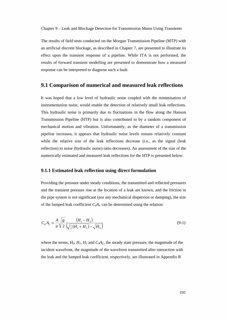
where the terms, H0, H1, H2 and CdAL, the steady state pressure, the magnitude of the
incident wavefront, the magnitude of the wavefront transmitted after interaction with
the leak and the lumped leak coefficient, respectively, are illustrated in Appendix R

Chapter 9 – Leak and Blockage Detection for Transmission Mains Using Transients
192
Equation 9-1 can be rearranged to form Equation 9-2 (below) which can be solved
iteratively to determine a value for H2 and the maximum anticipated leak reflection
when friction and other mechanical effects are ignored:
( )( )( ) =−
−+−
Ld ACHHH
HHg
a
A
02121
21
20 (9-2)
The leak on the Hanson Transmission Pipeline (HTP) was simulated using the
galvanised pipe section connected to an existing fire plug/air valve as described in
Chapter 6. The geometry of the galvanised steel pipe section and height of vertical
leak discharge were used to estimate the initial vertical velocity of the leak jet and
hence a discharge of approximately 9L/s. This was confirmed, as described in
Appendix T, using the orifice equation and geometric details of the fire plug/air valve
(including the geometry of the seat of the valve). Finally, chart records from the
insertion flowmeter in the HTP, included in Appendix J, confirmed that an additional
9L/s discharge occurred in the HTP when the fire plug/air valve was partially opened.
Knowing that the seat of the fire plug/air valve was opened 6.5 of 10 turns, giving and
equivalent orifice diameter of approximately 25mm across the seat of the valve, the
CdAL for the simulated leak on the Hanson Transmission Pipeline (HTP) is
approximately 0.000295m2 (for a Cd of approximately 0.6). The orifice equation can
be used to calculate the initial pressure at the leak location:
=⎟⎟⎠
⎞⎜⎜⎝
⎛=
2
0 2
1
Ld
L
AC
Q
gH 47.46m
Furthermore, the Joukowsky pressure rise can be estimated, for the customised 50mm
ball valve mounted in the transient generator, as described in Chapter 6, after it is
closed over approximately 10ms to induce a transient through an existing 200mm
diameter scour valve mounted on the side of the HTP. Based on a flow rate through
the transient generator of 43L/s, the theoretical Joukowsky pressure rise can be
calculated:

Chapter 9 – Leak and Blockage Detection for Transmission Mains Using Transients
193
=∆×−=∆g
VaH 15.06m
where 1055=a m/s and 14.0−=∆V m/s
The pressure rise is split equally as the transient propagates from the scour valve into
the HTP such that an increase in pressure of approximately 7.53m (HJ) occurs
upstream and downstream of the point of generation. As confirmed below, this
theoretical pressure rise is approximately equal to that observed in the measured
responses.
Given the area of the HTP is approximately 0.3072m2, its wave speed is 1055m/s, H0
is equal to 47.46m, H1 (= H0 + HJ) is equal to 54.99m and, finally, CdAL is equal to
0.000295m2, the pressure after the leak reflection can be calculated as H2 equal to
54.75m giving a leak reflection size of 0.24m. This is a maximum estimate of the size
of the leak reflection ignoring the effects of fluid friction and mechanical dispersion
and damping.
9.1.2 Estimated leak reflection using a forward transient model
Equation 9-1 can only provide a maximum estimate of the size of a leak reflection in
pipelines without significant friction or other dispersion and damping phenomena.
The Hanson Transmission Pipeline (HTP) is a relatively long field pipeline with,
amongst other things, significant friction loss and so it is more accurate to estimate the
size of anticipated leak reflections using a forward transient model that includes the
effect of friction. Numerous forms of forward transient model have been identified
and calibrated in Chapters 7 and 8. A forward transient model with unsteady friction,
but without any mechanical “viscous” mechanism, will be used for the purpose of
estimating the reflections for various leak sizes on the HTP. A roughness value of
2mm will be used for both the HTP and offtake branch.
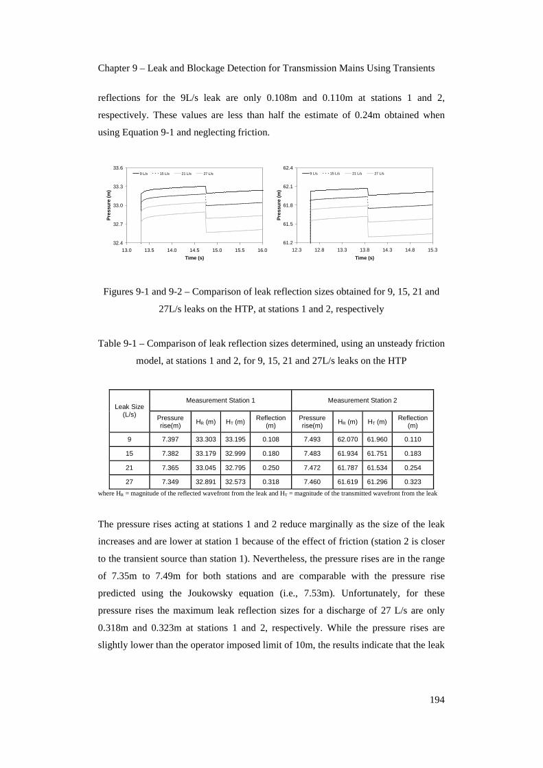
Figures 9-1 and 9-2 show the size of the reflections for 9, 15, 21 and 27L/s leaks, with
CdAL values of 0.000295, 0.000484, 0.000678 and 0.000873m2, respectively. The
sizes of the leak reflections are listed in Table 9-1. Importantly, the sizes of the
Chapter 9 – Leak and Blockage Detection for Transmission Mains Using Transients
194
reflections for the 9L/s leak are only 0.108m and 0.110m at stations 1 and 2,
respectively. These values are less than half the estimate of 0.24m obtained when
using Equation 9-1 and neglecting friction.
32.4
32.7
33.0
33.3
33.6
13.0 13.5 14.0 14.5 15.0 15.5 16.0
Time (s)
Pre
ssu
re (
m)
9 L/s 15 L/s 21 L/s 27 L/s
61.2
61.5
61.8
62.1
62.4
12.3 12.8 13.3 13.8 14.3 14.8 15.3
Time (s)
Pre
ssu
re (
m)
9 L/s 15 L/s 21 L/s 27 L/s
Figures 9-1 and 9-2 – Comparison of leak reflection sizes obtained for 9, 15, 21 and
27L/s leaks on the HTP, at stations 1 and 2, respectively
Table 9-1 – Comparison of leak reflection sizes determined, using an unsteady friction
model, at stations 1 and 2, for 9, 15, 21 and 27L/s leaks on the HTP
Measurement Station 1 Measurement Station 2 Leak Size
(L/s) Pressure rise(m) HR (m) HT (m) Reflection
(m) Pressure rise(m) HR (m) HT (m) Reflection
(m)
9 7.397 33.303 33.195 0.108 7.493 62.070 61.960 0.110
15 7.382 33.179 32.999 0.180 7.483 61.934 61.751 0.183
21 7.365 33.045 32.795 0.250 7.472 61.787 61.534 0.254
27 7.349 32.891 32.573 0.318 7.460 61.619 61.296 0.323
where HR = magnitude of the reflected wavefront from the leak and HT = magnitude of the transmitted wavefront from the leak
The pressure rises acting at stations 1 and 2 reduce marginally as the size of the leak
increases and are lower at station 1 because of the effect of friction (station 2 is closer
to the transient source than station 1). Nevertheless, the pressure rises are in the range
of 7.35m to 7.49m for both stations and are comparable with the pressure rise
predicted using the Joukowsky equation (i.e., 7.53m). Unfortunately, for these
pressure rises the maximum leak reflection sizes for a discharge of 27 L/s are only
0.318m and 0.323m at stations 1 and 2, respectively. While the pressure rises are
slightly lower than the operator imposed limit of 10m, the results indicate that the leak

Chapter 9 – Leak and Blockage Detection for Transmission Mains Using Transients
195
reflection information that can be induced in pipelines such as the HTP will be
relatively weak.
It is important to confirm that the predicted pressure rises are comparable with those
observed in the measured responses. Table 9-2 shows the average pressure for 1s prior
to and following the induction of the controlled transients for tests 1 (without leakage)
and 3 (with the artificial leak). The pressure for test 1 rises by an average of 7.40m
(for stations 1 and 2). The pressure for test 3 rises by an average of 7.28m. The
pressure rises predicted without and with the leak are of the same order as those
predicted using the transient model (they are marginally lower). Discrepancies may be
attributed to local variations in friction and mechanical damping effects.
Table 9-2 – Transient overpressures from measured responses for tests 1 and 3
Measurement Station 1 Measurement Station 2 Test No. Steady
(m) Plateau
(m) Pressure Rise
(m) Steady
(m) Plateau
(m) Pressure Rise
(m)
Average Pressure Rise (m)
1 25.94 33.32 7.38 54.80 62.21 7.41 7.40
3 25.80 33.06 7.26 54.50 61.80 7.30 7.28
9.1.3 Measured leak reflection from Hanson Transmission Pipeline
Figures 9-3 and 9-4 show the measured leak reflections for test 3 at stations 1 and 2,
respectively. The predicted leak reflections, respectively 0.108m and 0.110m, are
superimposed for the purpose of comparison. It is apparent that the leak reflections
are barely discernable amongst background hydraulic noise. Given the conclusions of
Stoianov et al. (2003a), regarding small leak reflections and large diameter pipelines,
the result is not unexpected. The results for Covas et al. (2004a) stand in contrast but
can be explained by the fact that the pipeline tested was only 300mm in diameter, had
a very high static pressure (132m) and was subjected to a pressure rise (13.2m) above
the limits determined by both Stoianov et al. (2003a) and in this research.

Chapter 9 – Leak and Blockage Detection for Transmission Mains Using Transients
196
31.9
32.5
33.1
33.7
34.3
14.25 14.45 14.65 14.85 15.05 15.25
Time (s)
Pre
ssu
re (
m)
Measured response - station 1
Predicted response - station 1
Leak reflection
60.6
61.2
61.8
62.4
63.0
13.35 13.55 13.75 13.95 14.15 14.35
Time (s)
Pre
ssu
re (
m)
Measured response - station 2
Predicted response - station 2
Leak reflection
Figures 9-3 and 9-4 – Measured versus predicted leak reflections for test 3, conducted
on the HTP, at stations 1 and 2, respectively
Figures 9-5 and 9-6 show the measured and predicted leak reflections in more detail.
A marginal fall in the measured response is discernable at the location of the leak. The
average pressures for 0.5s prior to and following the time of the leak reflection, for
test 3 at station 1, are 33.092m and 32.989m, respectively. This gives an average drop
of 0.103m. For station 2, the average pressures are 61.789 and 61.693m giving an
average drop of 0.096m. These measurements are inconsistent with the expectation
that the measured reflection at station 2, located closer to the transient generator and
artificial leak, should be greater than that at station 1.
32.8
32.9
33.0
33.1
33.2
33.3
14.5 14.6 14.7 14.8 14.9 15.0 15.1
Time (s)
Pre
ssu
re (
m)
Measured response - station 1
Predicted response - station 1
61.5
61.6
61.7
61.8
61.9
62.0
13.6 13.7 13.8 13.9 14.0 14.1 14.2
Time (s)
Pre
ssu
re (
m)
Measured response - station 2
Predicted response - station 2
Figures 9-5 and 9-6 – Focus on measured versus predicted leak reflections for test 3,
conducted on the HTP, at stations 1 and 2, respectively
The results may indicate that mechanical dispersion and damping near the source of
the transient have a disproportionately greater effect. However, it may also be because
the reflection recorded at station 2 is obscured, to a greater degree than at station 1, by
localised hydraulic noise. The results confirm that, for the size of leak and maximum
Chapter 9 – Leak and Blockage Detection for Transmission Mains Using Transients
197
permissible pressure rise specified by South Australian system operators, weak leak
reflections occur in larger transmission pipelines.
The sources of the hydraulic noise are discussed in Chapter 10 and include flow
variability or “flutter” through the nozzle mounted in the transient generator,
particularly for the tests conducted in May 2004, interaction of the relatively sharp
wavefronts with wall lining (and wall) thickness and other material variations and
reflections from the saddle supports and collar restraints (and changes in pipeline
profile in elevation and plan). Once the side discharge valve mounted in the transient
generator has been closed, the effect of flow variability is greatly reduced leaving
reflections from wall lining (and wall) thickness changes and the saddle supports and
collar restraints as the main sources of the hydraulic noise. Unfortunately, for leak
sizes around the threshold of interest, the measured reflections are within the
hydraulic noise band giving a very low signal to noise ratio.
9.2 Problems with wavefront dispersion
9.2.1 Wavefront dispersion and transient models
Traditional transient models, which neglect the effects of unsteady friction and
mechanical dispersion and damping (and flexural and shear wave formation) do not
account for wavefront dispersion. This problem has not been previously contemplated
by researchers investigating hydraulic transient methods for fault detection because of
a lack of measured responses from field pipelines. As described in Chapter 7, the
measured responses from both the Hanson Transmission Pipeline (HTP) and the
Morgan Transmission Pipeline (MTP) exhibit significant dispersion that increases as
the induced wavefronts continue propagating within the pipeline. This dispersion will
progressively obscure reflection information from any leak along the pipelines.
This problem is distinct from the problem of hydraulic noise obscuring weak leak
reflections. In the case of tests 3 and 4, conducted on the HTP, the close proximity of
the transient generator, the artificial 9L/s leak and measurement station 2 are such that
the hydraulic noise described above has not dispersed at the times the initial leak
reflection is recorded at station 2. Furthermore, while the dispersion has increased in

Chapter 9 – Leak and Blockage Detection for Transmission Mains Using Transients
198
the measured responses observed at station 1 (located approximately 878m to the east
of the transient generator), both the hydraulic noise and weak leak reflection remain
discernable.
The wavefront dispersion considered in this section increases as the length of pipeline
over which the wavefronts travel increases. As shown in Chapter 7, this results in
considerable dispersion of the reflected wavefronts from the Hanson summit tanks
and closed butterfly valve at “Sheep Dip” that cannot be explained in terms of the
inertial effects described by Skalak (1956). Hence, both the hydraulic noise and the
weak leak reflections themselves are dispersed and the leaks remain relatively
obscured.
Transient models have been developed in Chapter 8 that include unsteady friction and
mechanical dispersion and damping. These models have been calibrated to the no-leak
responses from the HTP. However, as previously discussed, “viscous” mechanisms
only provide for equivalent dispersion and damping. They do not describe the
physical behaviour of a pipeline and are unable to replicate the precise structure of the
measured responses. Furthermore, while the damping in the measured response is, on
average, correctly predicted, the observed dispersion is not accurately approximated
over the initial stages of the transient, unless separate long and short term calibrations
are performed.
9.2.2 Use of prior information regarding leak size
The use of prior information, in the form of knowledge of the leak discharge, can
partially compensate for structural deficiencies in the forward transient models
presented in Chapter 8, including an inability to model significant dispersion over the
initial stages of a measured transient response as well as over the longer term, and/or
low sensitivity leak information.
Prior information regarding leak discharge can be used, during Inverse Transient
Analysis (ITA) to fix the size of a leak at each potential leak location. Hence, both the
location and the size of the leak are fixed, as each potential leak location is assessed,
leaving the determination of the goodness of the fit (i.e., the objective function) as the

Chapter 9 – Leak and Blockage Detection for Transmission Mains Using Transients
199
only variable. The results presented below, for both short and long term analysis,
without and with prior information regarding the leak discharge, have been
determined using the quasi-steady friction (QSF), the unsteady friction (UF) and the
unsteady friction and “viscous” Hanson pipeline and offtake branch (UFVHOB)
models as previously developed and calibrated in Chapter 8.
9.2.3 Use of leak damping information
While the reflections from the artificial 9L/s leak introduced to the Hanson
Transmission Pipeline (HTP) are difficult to discern amongst significant hydraulic
noise, the long term measured responses nevertheless exhibit significant leak related
damping. Figures 9-7 and 9-8 show the numerically estimated effect, over the long
term, of 9, 15, 21 and 27L/s leaks at the location of the simulated leak on the HTP, at
measurement stations 1 and 2, respectively (the measured responses from the HTP for
tests 3 and 4 exhibit similar damping, as shown below, for a 9L/s leak).
10
15
20
25
30
35
40
45
0 100 200 300 400 500 600
Time (s)
Pre
ssu
re (
m)
9 L/s 15 L/s 21 L/s 27 L/s
39
44
49
54
59
64
69
74
0 100 200 300 400 500 600
Time (s)
Pre
ssu
re (
m)
9 L/s 15 L/s 21 L/s 27 L/s
Figures 9-7 and 9-8 – Comparison of leak damping for 9, 15, 21 and 27L/s leaks on
HTP, at stations 1 and 2, respectively
The leak damping significantly increases with the size of the leak. Furthermore, the
leak damping effect is more significant than the damping associated with unsteady
friction and mechanical dispersion and damping. This confirms that important leak
damping information is available in the measured responses from the HTP. The
challenge, is applying transient response analysis or Inverse Transient Analysis (ITA),
to interpret this leak related damping information.

Chapter 9 – Leak and Blockage Detection for Transmission Mains Using Transients
200
9.3 Leak detection using quasi-steady friction (QSF) model
9.3.1 Results of Inverse Transient Analysis performed over 580s
Given that the quasi-steady friction (QSF) model was only calibrated over the long
term (580s), Inverse Transient Analysis (ITA) will only be performed, to locate and
size the artificially introduced 9L/s leak, using long term measured responses. Figures
9-9 and 9-10 show the logarithm of the ratios between the objective functions
determined for each potential leak location and the minimum objective function
obtained when ITA is performed by fixing the leak location at individual nodes along
the Hanson Transmission Pipeline (HTP) and then fitting for the optimum leak size,
without and with prior information regarding the leak discharge, respectively.
0
0.05
0.1
0.15
0.2
0.25
0.3
0.35
0.4
41 81 121
161
201
241
281
321
361
401
441
481
521
561
601
Leak Node
Lo
g o
f ra
tio
O/F
to
O/F
min
Objective function ratios for test 3 with no prior information
Continuous envelope
0
0.1
0.2
0.3
0.4
0.5
0.6
0.7
0.8
0.9
41 81 121
161
201
241
281
321
361
401
441
481
521
561
601
Leak Node
Lo
g o
f ra
tio
O/F
to
O/F
min
Objective function ratios for test 3 with prior information
Continuous envelope
Figures 9-9 and 9-10 – Using the QSF model, calibrated over the long term, to
perform long term ITA for test 3, without and with prior information, respectively
Figure 9-9 shows that, without prior information regarding the leak discharge, the
minimum objective function is obtained when the leak location is fixed at node 401.
The objective function when the leak is fixed at its “true” location (node 441) is
ranked 6th from the minimum value for the leak at node 401. There is a significant
difference between the fitted leak sizes, at nodes 401 and 441, of 0.000527m2 and
0.000474m2, respectively. The fitted leak size at node 441 is closer to the “true” leak
size of 0.000295m2. Figure 9-10 shows that, with prior information regarding the leak
discharge, the minimum objective function is obtained when the leak location is fixed
at node 361. The objective function when the leak is fixed at its “true” location (node
441) is ranked 3rd from the minimum value. This represents an improvement relative
to the results obtained without prior information regarding the leak discharge.

Chapter 9 – Leak and Blockage Detection for Transmission Mains Using Transients
201
Figures 9-11 and 9-12 show the measured and predicted responses at station 1, over a
time scale of 580s, when the leak is located at its “true” position (node 441), and ITA
is performed without and with prior information regarding the leak discharge,
respectively. Figure 9-11 confirms that the QSF model does not replicate non-leak
related dispersion. However, the measured damping is approximated because a leak
size of 0.000474m2 is erroneously fitted (compared to the “true” leak size of
0.000295m2). Figure 9-12 shows that, by fixing the leak size to its “true” value, the
measured damping cannot be replicated by inaccurately calibrating for the size of the
leak and the structural inadequacy in the QSF model is exposed. This example shows
how fitting a parameter (in this case, the size of a leak rather than pipe roughness) can
incorrectly compensate for other phenomena affecting a transient response.
10
15
20
25
30
35
40
45
0 100 200 300 400 500 600Time (s)
Pre
ssu
re (
m)
Measured response at station 1
Predicted response at station 1
10
15
20
25
30
35
40
45
0 100 200 300 400 500 600Time (s)
Pre
ssu
re (
m)
Measured response at station 1
Predicted response at station 1
Figures 9-11 and 9-12 – Comparison between measured and predicted responses, over
580s, when ITA is performed without and with prior information, respectively
Figures 9-13 and 9-14 show the measured and predicted responses at station 1, over a
time scale of 40s, when the leak is located at its “true” position (node 441), and ITA is
performed without and with prior information regarding the leak discharge,
respectively. Figure 9-13 shows a discrepancy between the measured and predicted
steady state pressures due to the erroneously fitted leak size. Figure 9-14 shows that,
by constraining the leak size to its “true” value, the error between the measured and
predicted steady state pressures is reduced. Figures 9-13 and 9-14 confirm that the
measured and predicted leak reflection information is relatively indistinct in the
context of the observed hydraulic noise and dispersion.

Chapter 9 – Leak and Blockage Detection for Transmission Mains Using Transients
202
24
27
30
33
36
39
42
0 8 16 24 32 40Time (s)
Pre
ssu
re (
m)
Measured response at station 1
Predicted response at station 1
24
27
30
33
36
39
42
0 8 16 24 32 40Time (s)
Pre
ssu
re (
m)
Measured response at station 1
Predicted response at station 1
Figures 9-13 and 9-14 – Comparison between measured and predicted responses, over
40s, when ITA is performed without and with prior information, respectively
9.3.2 Regression diagnostics for the QSF model following ITA
Figures 9-15 and 9-16 show the standardised residual plotted against time for Inverse
Transient Analysis (ITA) performed without and with prior information regarding the
leak discharge. The leak is located at its “true” location (i.e., node 441). Prime facie,
the deterioration in the residual error when the prior information is used suggests that
the fixed (“true”) leak size is incorrect. However, the correct interpretation is that the
leak damping should not be used to compensate for the effects of other phenomena
and that the quasi-steady friction (QSF) model is structurally inadequate.
-6
-4
-2
0
2
4
6
0 100 200 300 400 500 600
Time (s)
Sta
nd
ard
ised
res
idu
al
Ideal standardised residual vs time
Standardised residual vs time
-6
-4
-2
0
2
4
6
0 100 200 300 400 500 600
Time (s)
Sta
nd
ard
ised
res
idu
al
Ideal standardised residual vs time
Standardised residual vs time
Figures 9-15 and 9-16 – Standardised residual versus time plots for test 3, when using
the QSF model, without and with prior information, respectively

Chapter 9 – Leak and Blockage Detection for Transmission Mains Using Transients
203
9.4 Leak detection using unsteady friction (UF) model
9.4.1 Results of Inverse Transient Analysis performed over 580s
As for the analysis performed using the quasi-steady friction (QSF) model, Inverse
Transient Analysis (ITA) will only be performed, using the unsteady friction (UF)
model, to locate and size the artificially introduced 9L/s leak using the long term
measured responses. Figures 9-17 and 9-18 show the logarithm of the ratios between
the objective functions determined for each potential leak location and the minimum
objective function obtained when ITA is performed by fixing the leak location at
individual nodes along the Hanson Transmission Pipeline (HTP) and then fitting for
the optimum leak size, without and with prior information regarding the leak
discharge, respectively.
0
0.05
0.1
0.15
0.2
0.25
0.3
0.35
0.4
41 81 121
161
201
241
281
321
361
401
441
481
521
561
601
Leak Node
Lo
g o
f ra
tio
O/F
to
O/F
min
Objective function ratios for test 3 with no prior information
Continuous envelope
0
0.1
0.2
0.3
0.4
0.5
0.6
0.7
0.8
0.9
41 81 121
161
201
241
281
321
361
401
441
481
521
561
601
Leak Node
Lo
g o
f ra
tio
O/F
to
O/F
min
Objective function ratios for test 3 with prior information
Continuous envelope
Figures 9-17 and 9-18 – Using the UF model, calibrated over the long term, to
perform long term ITA for test 3, without and with prior information, respectively
Figure 9-17 shows that, without prior information regarding the leak discharge, the
minimum objective function is obtained when the leak location is fixed at node 201.
The objective function when the leak is fixed at its “true” location (node 441) is
ranked 7th from the minimum value for the leak at node 201. This represents a
deterioration relative to the results obtained using the QSF model. There is a
significant difference between the fitted leak sizes, at nodes 201 and 441, of
0.000777m2 and 0.000333m2, respectively. The fitted leak size at node 441 is
relatively close to the “true” leak size of 0.000295m2. Figure 9-18 shows that, with
prior information regarding the leak discharge, the minimum objective function is
obtained when the leak location is fixed at node 321. The objective function when the
Chapter 9 – Leak and Blockage Detection for Transmission Mains Using Transients
204
leak is fixed at its “true” location (node 441) is ranked 2rd from the minimum value.
This represents an improvement relative to the results obtained without prior
information regarding the leak discharge and to those obtained using the QSF model.
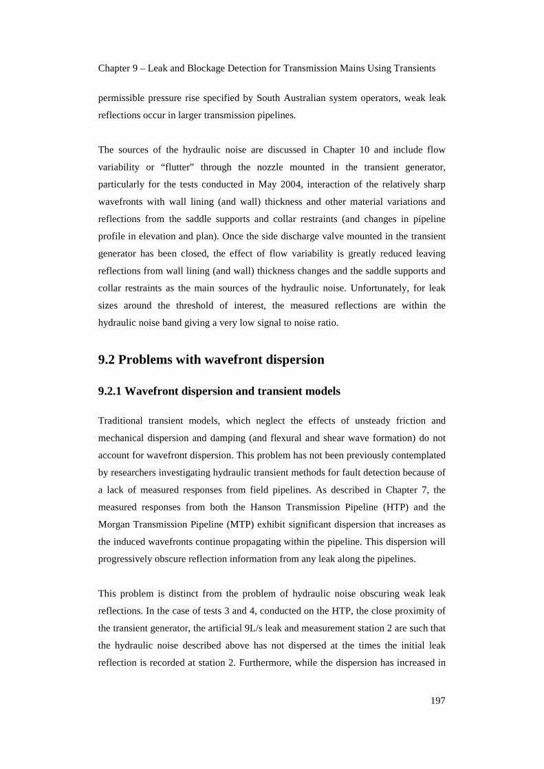
9.4.2 Regression diagnostics for the UF model following ITA
Figures 9-19 and 9-20 show the standardised residual plotted against time for Inverse
Transient Analysis (ITA) performed without and with prior information regarding the
leak discharge. The leak is located at its “true” location (i.e., node 441). In contrast to
the results obtained using the quasi-steady friction (QSF) model (presented for
comparison), the cyclical error apparent in the residual reduces with increasing time
regardless of whether prior information regarding the leak size is used. Furthermore,
there is only a marginal difference between the residual obtained without and with
prior information. This is a consequence of the similarity between the fitted and “true”
leak sizes specified above.
-6
-4
-2
0
2
4
6
0 100 200 300 400 500 600
Time (s)
Sta
nd
ard
ised
res
idu
al
Ideal standardised residual vs time
Standardised residual vs time - QSF model
Standardised residual vs time - UF model
-6
-4
-2
0
2
4
6
0 100 200 300 400 500 600
Time (s)
Sta
nd
ard
ised
res
idu
al
Ideal standardised residual vs time
Standardised residual vs time - QSF model
Standardised residual vs time - UF model
Figures 9-19 and 9-20 – Standardised residual versus time plots for test 3, when using
the UF model, without and with prior information, respectively
9.5 Leak detection using “viscous” UFVHOB model
9.5.1 Results of Inverse Transient Analysis performed over 580s
As for the Inverse Transient Analysis (ITA) performed using the quasi-steady friction
(QSF) and unsteady friction (UF) models, ITA will be performed, using the unsteady
friction and “viscous” Hanson pipeline and offtake branch (UFVHOB) model, to
locate and size the artificially introduced 9L/s leak using the long term measured

Chapter 9 – Leak and Blockage Detection for Transmission Mains Using Transients
205
responses. Figures 9-21 and 9-22 show the logarithm of the ratios between the
objective functions determined for each potential leak location and the minimum
objective function obtained when ITA is performed by fixing the leak location at
individual nodes along the Hanson Transmission Pipeline (HTP) and then fitting for
the optimum leak size, without and with prior information regarding the leak
discharge, respectively.
0
0.05
0.1
0.15
0.2
0.25
0.3
0.35
0.4
41 81 121
161
201
241
281
321
361
401
441
481
521
561
601
Leak Node
Lo
g o
f ra
tio
O/F
to
O/F
min
Objective function ratios for test 3 with no prior information
Continuous envelope
0
0.1
0.2
0.3
0.4
0.5
0.6
0.7
0.8
0.9
41 81 121
161
201
241
281
321
361
401
441
481
521
561
601
Leak Node
Lo
g o
f ra
tio
O/F
to
O/F
min
Objective function ratios for test 3 with prior information
Continuous envelope
Figures 9-21 and 9-22 – Using the UFVHOB model, calibrated over the long term, to
perform long term ITA for test 3, without and with prior information, respectively
Figure 9-21 shows that, without prior information regarding the leak discharge, the
minimum objective function is obtained when the leak location is fixed at node 201.
The objective function when the leak is fixed at its “true” location (node 441) is
ranked 8th from the minimum value for the leak at node 201. This represents a
deterioration relative to the results obtained using the QSF and UF models. There is a
significant difference between the fitted leak sizes, at nodes 201 and 441, of
0.000768m2 and 0.000328m2, respectively. The fitted leak size at node 441 is
relatively close to the “true” leak size of 0.000295m2. Figure 9-22 shows that, with
prior information regarding the leak discharge, the minimum objective function is
obtained when the leak location is fixed at node 321. The objective function when the
leak is fixed at its “true” location (node 441) is ranked 2rd from the minimum value.
Figure 9-23 shows the measured and predicted responses at station 1, over a time
scale of 580s, when the leak is located at its “true” position (node 441), and ITA is
performed without prior information regarding the leak discharge. The measured
response is best replicated when an erroneous leak size of 0.000328m2 is fitted

Chapter 9 – Leak and Blockage Detection for Transmission Mains Using Transients
206
(compared to the “true” leak size of 0.000295m2). As for the results obtained using
the QSF model, this indicates that the fitted leak size is acting to compensate for non-
leak related damping.
10
15
20
25
30
35
40
45
0 100 200 300 400 500 600Time (s)
Pre
ssu
re (
m)
Measured response at station 1
Predicted response at station 1
Figure 9-23 – Comparison between measured and predicted responses, over 580s,
when the leak is located at node 441, and ITA is performed without prior information
9.5.2 Regression diagnostics for the UFVHOB model following ITA
Figures 9-24 and 9-25 show the standardised residual plotted against time for Inverse
Transient Analysis (ITA) performed without and with prior information regarding the
leak discharge. The leak is located at its “true” location (i.e., node 441). A marginal
reduction in the residuals is apparent relative to the results obtained using the
unsteady friction (UF) model (presented for comparison). However, a cyclical error
persists in the residuals regardless of whether prior information regarding the leak size
is used. Furthermore, there is only a marginal difference between the residual
obtained without and with prior information. Unfortunately, the cyclical residual is
significant and is related to the inability of the unsteady friction and “viscous” Hanson
pipeline and offtake branch (UFVHOB) model to replicate the dispersion and
damping over the later stages of the transient responses with sufficient accuracy. This

Chapter 9 – Leak and Blockage Detection for Transmission Mains Using Transients
207
inaccuracy is critical in the context of accessing the leak damping information in the
context of Inverse Transient Analysis (ITA).
-6
-4
-2
0
2
4
6
0 100 200 300 400 500 600
Time (s)
Sta
nd
ard
ised
res
idu
al
Ideal standardised residual vs time
Standardised residual vs time - UF model
Standardised residual vs time - UFVHOB model
-6
-4
-2
0
2
4
6
0 100 200 300 400 500 600
Time (s)
Sta
nd
ard
ised
res
idu
al
Ideal standardised residual vs time
Standardised residual vs time - UF model
Standardised residual vs time - UFVHOB model
Marginally greater residuals relative to those obtained without prior information
Figures 9-24 and 9-25 – Standardised residual versus time plots for test 3, when using
the UFVHOB model, without and with prior information, respectively
9.6 Using UFVHOB model over a period of 2L/a seconds
9.6.1 Results of ITA performed over 2L/a seconds
Based on the model calibration performed in Chapter 8, it is known that the unsteady
friction and “viscous” Hanson pipeline and offtake branch (UFVHOB) model,
calibrated over the long term, does not approximate the dispersion of the measured
responses, particularly over their initial stages, as accurately as when calibration is
performed over the short term. Inverse Transient Analysis (ITA) will therefore be
performed, using the UFVHOB model calibrated over the short term, to locate and
size the artificially introduced leak using 2L/a seconds (38.1s) of the measured
responses. Figures 9-26 and 9-27 show the logarithm of the ratios between the
objective functions determined for each potential leak location and the minimum
objective function obtained when ITA is performed by fixing the leak location at
individual nodes along the Hanson Transmission Pipeline (HTP) and then fitting for
the optimum leak size, without and with prior information regarding the leak
discharge, respectively.

Chapter 9 – Leak and Blockage Detection for Transmission Mains Using Transients
208
0
0.05
0.1
0.15
0.2
0.25
0.3
0.35
0.4
41 81 121
161
201
241
281
321
361
401
441
481
521
561
601
Leak Node
Lo
g o
f ra
tio
O/F
to
O/F
min
Objective function ratios for test 3 with no prior information
Continuous envelope
0
0.05
0.1
0.15
0.2
0.25
0.3
0.35
0.4
41 81 121
161
201
241
281
321
361
401
441
481
521
561
601
Leak Node
Lo
g o
f ra
tio
O/F
to
O/F
min
Objective function ratios for test 3 with prior information
Continuous envelope
Figures 9-26 and 9-27 – Using the UFVHOB model, calibrated over the short term, to
perform short term ITA for test 3, without and with prior information, respectively
Figure 9-26 shows that, without prior information regarding the leak discharge, the
minimum objective function is obtained when the leak location is fixed at node 241.
The objective function when the leak is fixed at its “true” location (node 441) is
ranked 5th from the minimum value for the leak at node 241. This represents a
significant improvement relative to the results obtained when long term ITA was
performed using the UFVHOB model. However, a significant difference persists
between the fitted leak sizes, at nodes 241 and 441, of 0.000649m2 and 0.000365m2,
respectively. The fitted leak size at node 441 is closer to the “true” leak size of
0.000295m2. Figure 9-27 shows that, with prior information regarding the leak
discharge, the minimum objective function is obtained when the leak location is fixed
at node 321. The objective function when the leak is fixed at its “true” location (node
441) is ranked 3rd from the minimum value. This is a deterioration relative to the
result obtained using the UFVHOB model calibrated over the long term.
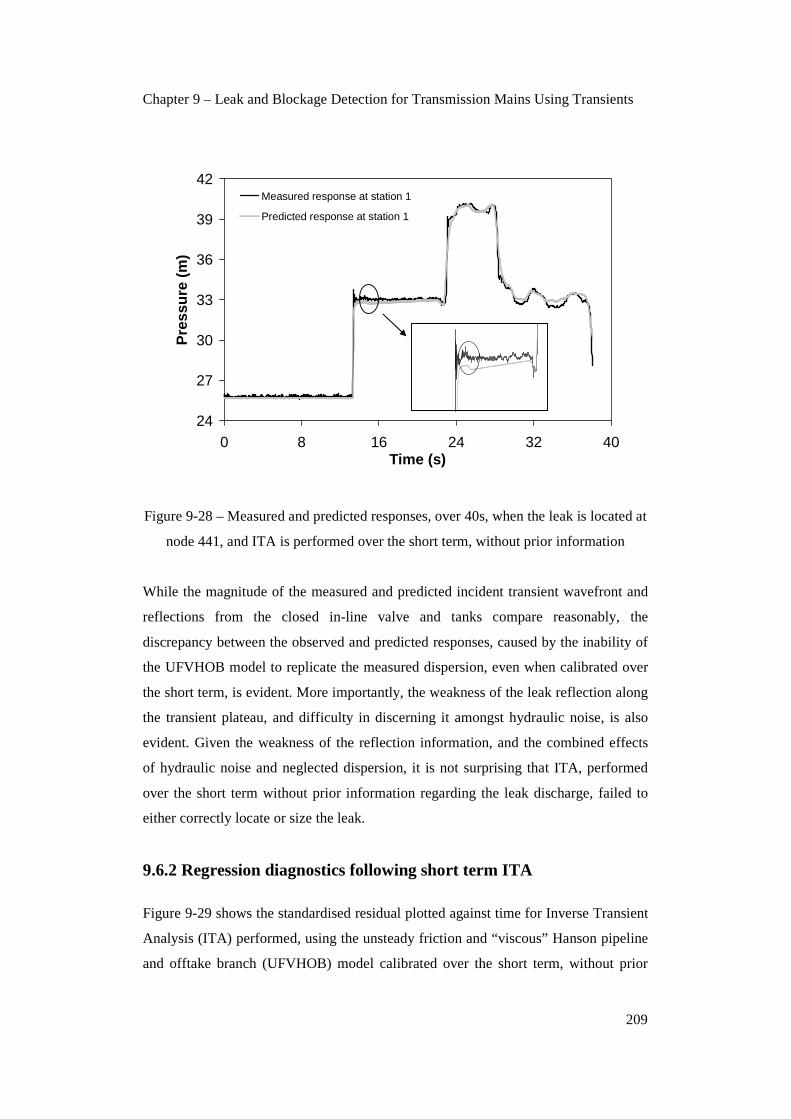
Figure 9-28 shows the measured and predicted responses at station 1, over a time
scale of 2L/a seconds (38.1s), when the leak is located at its “true” position (node
441), and ITA is performed, over the short term, without prior information regarding
the leak discharge. The measured response is best replicated when an erroneous leak
size of 0.000365m2 is fitted (based on objective function minimisation). The inset
shows that this erroneously fitted leak size results in an inaccurate offset of the
predicted steady state pressure and initial transient plateau below the measured
pressures. As for the long term ITA, the fitted leak size is compensating for non-leak
related uncertainties rather than giving a more accurate estimate of the leak size.
Chapter 9 – Leak and Blockage Detection for Transmission Mains Using Transients
209
24
27
30
33
36
39
42
0 8 16 24 32 40Time (s)
Pre
ssu
re (
m)
Measured response at station 1
Predicted response at station 1
Figure 9-28 – Measured and predicted responses, over 40s, when the leak is located at
node 441, and ITA is performed over the short term, without prior information
While the magnitude of the measured and predicted incident transient wavefront and
reflections from the closed in-line valve and tanks compare reasonably, the
discrepancy between the observed and predicted responses, caused by the inability of
the UFVHOB model to replicate the measured dispersion, even when calibrated over
the short term, is evident. More importantly, the weakness of the leak reflection along
the transient plateau, and difficulty in discerning it amongst hydraulic noise, is also
evident. Given the weakness of the reflection information, and the combined effects
of hydraulic noise and neglected dispersion, it is not surprising that ITA, performed
over the short term without prior information regarding the leak discharge, failed to
either correctly locate or size the leak.
9.6.2 Regression diagnostics following short term ITA
Figure 9-29 shows the standardised residual plotted against time for Inverse Transient
Analysis (ITA) performed, using the unsteady friction and “viscous” Hanson pipeline
and offtake branch (UFVHOB) model calibrated over the short term, without prior

Chapter 9 – Leak and Blockage Detection for Transmission Mains Using Transients
210
information regarding the leak discharge. The leak is located at its “true” location
(i.e., node 441). The discrepancies between the measured and predicted responses,
evident for the quasi-steady friction (QSF) and unsteady friction (UF) models, have
been reduced.
-6
-4
-2
0
2
4
6
0 8 16 24 32 40
Time (s)
Sta
nd
ard
ised
res
idu
al
Ideal standardised residual vs time
Standardised residual vs time
Ongoing discrepancies due to response of offtake branch
Figure 9-29 – Standardised residual versus time plot, for ITA over 2L/a seconds using
the UFVHOB model, calibrated over the short term, without prior information
9.7 Summary of problems affecting ITA for leak detection
Table 9-3 summarises the results of the Inverse Transient Analysis (ITA) performed
over the long term (i.e., 580s) using the quasi-steady friction (QSF), the unsteady
friction (UF) and the unsteady friction and “viscous” Hanson pipeline and offtake
branch (UFVHOB) models. Erroneous leak locations and sizes are determined,
without any prior information regarding the leak discharge, using the QSF, UF and
UFVHOB models. Erroneous leak locations are determined, when the leak size is
fixed using prior information regarding the leak discharge, using all three models.
Furthermore, the objective function does not minimise when the leak is fixed at its
“true” location and its size is determined without and with prior information regarding
the correct leak discharge.

Chapter 9 – Leak and Blockage Detection for Transmission Mains Using Transients
211
Table 9-3 – Comparison of results when ITA is performed over the long term
Without prior information With prior information
Model Calibration Leak
node/location Rank Size (m2) Leak node/location Rank Size (m2)
QSF Long term 401/8440m 1 0.000527 361/7596m 1 0.000295
QSF Long term 441/9284m 6 0.000474 441/9284m 3 0.000295
UF Long term 201/4220m 1 0.000777 321/6752m 1 0.000295
UF Long term 441/9284m 7 0.000333 441/9284m 2 0.000295
UFVHOB Long term 201/4220m 1 0.000768 321/6752m 1 0.000295
UFVHOB Long term 441/9284m 8 0.000328 441/9284m 2 0.000295
* true leak location taken as node 441 (CH 9284m) approximately equal to actual location at CH 9290m
Table 9-4 summarises the results of the ITA performed over the short term (i.e., 2L/a
seconds) using the UFVHOB model (calibrated to short term no-leak measured
responses). As for the ITA performed over the long term using a long term
calibration, an erroneous leak location and size is determined without any prior
information regarding the leak discharge. An erroneous leak location is determined
when the leak size is fixed using prior information regarding the leak discharge. The
objective function does not minimise when the leak is fixed at its “true” location and
its size is determined without and with prior information regarding the correct leak
discharge.
Table 9-4 – Comparison of results when ITA is performed over the short term
Without prior information With prior information
Model Calibration Leak
node/location Rank Size (m2) Leak node/location Rank Size (m2)
UFVHOB Short term 241/4220m 1 0.000649 321/6752m 1 0.000295
UFVHOB Short term 441/9284m 5 0.000365 441/9284m 3 0.000295
* true leak location taken as node 441 (CH 9284m) approximately equal to actual location at CH 9290m
9.7.1 Weak leak reflection information and hydraulic noise
As noted previously, the magnitude of the theoretically anticipated leak reflection,
neglecting friction, was approximately 0.24m. The inclusion of friction in a numerical

Chapter 9 – Leak and Blockage Detection for Transmission Mains Using Transients
212
transient model led to a reduction in the anticipated leak reflection to approximately
0.110m at station 2 (closest to the transient generator). The measured leak reflection
was approximately 0.096m at station 2. The reduction in the size of the numerically
predicted leak when unsteady friction is included in the numerical transient model
suggests that the effect of friction is significant and should not be ignored. The
residual difference between the size of the leak reflection predicted with unsteady
friction and the measured leak reflection suggests that additional phenomena, thought
to be related to mechanical dispersion and damping, may be further reducing the size
of the leak reflections.
The measured leak reflections are small and difficult to discern amongst significant
hydraulic noise. This hydraulic noise is thought to derive from a combination of the
effects of flow variability and mechanical motion and vibrations and/or reflections
from changes to the pipeline walls. As a consequence, the signal to noise ratio for the
leak to hydraulic noise is low and the latter acts to confound the optimisation of the
leak location and size when performing Inverse Transient Analysis (ITA). The ITA
becomes reliant upon low sensitivity steady state pressure information.
9.7.2 Effect of wavefront dispersion on damping information
Considerable dispersion of the measured wavefronts propagating along the Hanson
Transmission Pipeline (HTP) was observed for no-leak as well as leak tests.
Furthermore, the magnitude of the dispersion observed for all four tests was similar
suggesting that the dispersion was not leak related. It was hoped that the leak damping
information in the measured responses could be used to locate and size the artificial
9L/s leak introduced to the HTP if non-leak related sources of dispersion and damping
could be accounted for with sufficient accuracy using calibrated quasi-steady friction
(QSF), unsteady friction (UF) and unsteady friction and “viscous” Hanson pipeline
and offtake branch (UFVHOB) models.
While discrepancies in the replication of the no-leak measured response were reduced
significantly by the implementation of unsteady friction, and to a lesser degree,
calibration for mechanical dispersion and damping, the calibrated forward transient
models were not sufficiently accurate to enable the isolation of differences in leak

Chapter 9 – Leak and Blockage Detection for Transmission Mains Using Transients
213
damping related to different potential leak locations. This confirms that while the
effect of leak damping on a transient is significant, and will vary with the size of the
leak, there are many non-unique combinations of leak location and size that will give
rise to the same or similar damping effect. Uncertainties in pipeline roughness (or
friction effects) and the extent of mechanical dispersion and damping may prevent the
successful isolation of the damping effect of a particular leak (e.g., the 9L/s artificial
leak introduced to the HTP).
9.7.3 Use of prior information regarding leak discharge
Flowmeter records are often available for transmission pipelines (as they were for the
Hanson Transmission Pipeline (HTP)). The use of these records as prior information
regarding the magnitude of the leak discharge significantly constrained the solution
space during Inverse Transient Analysis (ITA) such that the identification of the
“true” leak was significantly improved despite the weakness of the leak reflection
information and the dispersion of leak damping information. That said, the use of
prior information regarding the leak size is a very significant concession in terms of
the potential for ITA for leak detection. In practical terms, South Australian Water
Corporation operators would have been able to identify the presence of the leak by
examining the flowmeter records and then visually inspecting the HTP.
9.8 Blockage detection in the Morgan Transmission Pipeline
In the case of transient response analysis and/or Inverse Transient Analysis (ITA) for
leak detection, South Australian Water Corporation operators were consulted to
determine the threshold size of interest for leak detection using hydraulic transients.
Field tests on the Hanson Transmission Pipeline (HTP) were then conducted to
determine whether leaks near the threshold of interest could, in fact, be successfully
located and sized. It is tempting to trivialise the inverse problem, particularly during
the early stages of the transfer of techniques using hydraulic transients for fault
detection to the field, by introducing a severe fault to a pipeline. The effect is that
problems afflicting transient model accuracy become less significant as the signal to
hydraulic noise ratio is increased.

Chapter 9 – Leak and Blockage Detection for Transmission Mains Using Transients
214
The introduction of a discrete blockage to the Morgan Transmission Pipeline (MTP),
as described in Chapter 6, demonstrates how a severe fault is easier to detect using
transient response analysis and/or ITA. As reported in Chapter 7, transient field tests
were conducted with in-line gate valve “No.3” along the MTP closed 54 of 58 turns.
This left an open aperture with an equivalent orifice diameter of approximately
50mm. In a pumped transmission pipeline, such as the MTP, a blockage of this
severity would become immediately apparent and could not form gradually. It is
difficult to envisage the circumstances under which such a blockage might form and
fortunately one never has along the MTP. As a consequence, the simulation of a
discrete blockage of the severity described above was considered unrealistic.
Figures 9-30 and 9-31 show the comparison between the measured and predicted
response of the MTP, over relatively short time periods, with a 50mm equivalent
diameter in-line orifice located at in-line valve “No.3”, at stations 1 and 2,
respectively. A relatively strong reflection (approximately 2.5m as recorded at station
1) is apparent because of the severity of the discrete blockage, and this reflection is far
greater than the magnitude of the hydraulic noise band. As a consequence, the
location and size of the discrete blockage are obvious and can be replicated with little
effort by simply conducting trial and error modelling with different blockage locations
and sizes. Figure 9-31 shows that the corresponding transmitted wavefront can also be
relatively easily modelled.
63
65
67
69
71
73
75
24 25 26 27 28 29 30Time (s)
Pre
ssu
re (
m)
Measured response at station 1
Predicted response at station 1
Timing and magnitude of initial reflection from partially closed in-line gate valve approximately predicted by including 50mm orifice at gate valve "No.3"
51
53
55
57
59
61
63
26 29 32 35 38 41 44Time (s)
Pre
ssu
re (
m)
Measured response at station 2
Predicted response at station 2
Initial partially transmitted wavefront
Reflection from gate valve "No.1" of initial transmitted wavefront and secondary reflection from gate valve "No.3"
Additional "hydraulic noise" from flow "flutter"
Figures 9-30 and 9-31 – Measured and predicted reflected and transmitted wavefronts,
from a discrete blockage, at stations 1 (over 6s) and 2 (over 18s), respectively

Chapter 9 – Leak and Blockage Detection for Transmission Mains Using Transients
215
Figures 9-32 and 9-33 show the comparison between the measured and predicted
response of the MTP, over a longer time period of 540s, with a 50mm equivalent
diameter in-line orifice located at in-line valve “No.3”, at stations 1 and 2,
respectively. It is apparent that the severity of the discrete blockage gives rise to a
significant damping effect upon the measured and predicted responses of the MTP
and a distinct secondary oscillation.
50
55
60
65
70
75
80
0 90 180 270 360 450 540Time (s)
Pre
ssu
re (
m)
Measured response at station 1
Measured response at station 1
In-situ air pocket reflectionUnpredicted damping due to lack of calibration for roughness and inelastic losses and neglect of entrained air
40
45
50
55
60
65
70
0 90 180 270 360 450 540Time (s)
Pre
ssu
re (
m)
Measured response at station 2
Predicted response at station 2
In-situ air pocket reflection Unpredicted damping due to lack of calibration for roughness and inelastic losses and neglect of entrained air
Figures 9-32 and 9-33 – Measured and predicted reflected and transmitted waveforms,
from a discrete blockage, at stations 1 and 2, respectively (over 540s)
While the blockage induced damping and secondary oscillation is dominant, a
discrepancy, exists between the measured and predicted damping and waveforms.
This is probably due to the effect of friction losses (pipeline roughness) and
mechanical dispersion and damping that have not been calibrated to no-blockage
responses (and possibly the presence of a small percentage of entrained air).
Nevertheless, the damping and secondary oscillation due to the presence of the
blockage are obvious and have been reasonably replicated, with no calibration effort,
by conducting trial and error modelling with different blockage locations and sizes.
The same blockage location and size gives the best fit over the short and long term
response of the MTP.
9.9 Summary
The size of the reflections from a range of leaks have been numerically assessed in
this chapter, for large transmission pipelines, and compared with the size of the
measured reflection from an artificial 9L/s leak introduced to the Hanson
Transmission Pipeline (HTP). It was found, by comparing results obtained using a

Chapter 9 – Leak and Blockage Detection for Transmission Mains Using Transients
216
frictionless reflection formulation and a forward transient model including unsteady
friction, that the effect of friction, and, to a lesser extent, mechanical dispersion and
damping, significantly reduce the size of leak reflections. The measured reflection
from the 9L/s leak was of the order of 0.1m and difficult to discern amongst
background hydraulic noise. Furthermore, significant dispersion of the leak reflected
wavefront reduced the effective interpretation of reflection and damping information
from the 9L/s leak.
The quasi-steady friction (QSF), unsteady friction (UF) and unsteady friction and
“viscous” Hanson pipeline and offtake branch (UFVHOB) models, developed and
calibrated in Chapter 8, have been used to perform Inverse Transient Analysis (ITA)
for leak detection. Furthermore, regression diagnostics, including, in particular,
standardised residual versus time plots, were used to assess the performance of each
forward transient model. ITA was performed over both the long and short term, using
the UFVHOB model, to assess the sensitivity of the results to the length of measured
response and to the proportion of reflection versus damping information. The QSF
model performed least well, in terms of correctly identifying the 9L/s leak, while the
UFVHOB model gave the best results. However, none of the proposed models
correctly identified the leak location or size. The use of prior information regarding
the leak discharge was proposed to compensate for the weakness of the direct leak
reflection and dispersion of reflection and damping information. This improved the
results of the ITA but the leak location and size were still not correctly identified.
The QSF and UF models were expected to perform less well given neglected
mechanical dispersion and damping. The UFVHOB model, although incorporating a
calibrated “viscous” mechanism, only provided for equivalent dispersion and damping
and did not accurately replicate the hydraulic noise and wavefront dispersion
obscuring the leak reflection information. The weakness of the leak reflection, relative
to background hydraulic noise, and the dispersion of leak reflection and damping
information were identified as the main reasons for the failure of the ITA.
If leak reflections in or near the band of hydraulic noise identified in this study are to
be used to successfully perform ITA then a more comprehensive understanding of the
phenomena contributing to the hydraulic noise is required. The mechanisms calibrated

Chapter 9 – Leak and Blockage Detection for Transmission Mains Using Transients
217
to replicate mechanical dispersion and damping make an “on-average” correction and
do not replicate the actual physical mechanisms at work (e.g., at individual restraints).
As a consequence, the calibrated quasi-steady friction (QSF), unsteady friction (UF)
and unsteady friction and “viscous” Hanson pipeline and offtake branch (UFVHOB)
models do not replicate the microstructure response over, in particular, the initial
stages of the measured transient responses. The microstructure response of the
Morgan Transmission Pipeline (MTP) will be examined in Chapter 10 to determine
whether variations in the condition of the pipeline wall help to explain the hydraulic
noise observed in the measured responses.
Another interesting reality is that the closer the leak is to the source of the induced
transient, the more significant will be the effect of obscuring hydraulic noise from, in
particular, mechanical motion and vibration. However, the further the leak is from the
source of the induced transient, the more significant will be the effect of progressive
dispersion which, unfortunately, also has the effect of obscuring the leak reflection by
broadening its associated wavefront. While the way in which the leak reflection is
obscured by hydraulic noise and dispersion differ, the common effect is to decrease
the accessibility of the leak reflection information in the measured response. This
insight is critical to the design of future field investigations seeking to develop
methods for leak detection using hydraulic transients.
Chapter 10 – Wall Condition Assessment for Transmission Mains Using Transients
218
Chapter10
Wall Condition Assessment for Transmission Mains
Using Transients
_____________________________________________________________________
The results presented in Chapter 9 identify hydraulic noise that cannot be explained
using either a complex forward transient model, incorporating unsteady friction,
entrained air and fluid structure interaction effects, or a conceptual model based on
the calibration of a “viscous” mechanism to approximate equivalent mechanical
dispersion and damping. This hydraulic noise is a significant problem if transient
response analysis and Inverse Transient Analysis (ITA) are to be used to identify
specific faults along transmission pipelines. Furthermore, it is not known whether the
hydraulic noise is associated with mechanical motion and vibration, or if there is some
other physical explanation, or a combination of both.
Misiunas et al. (2005) hypothesised that there was a correlation between an increase
in the standard deviation of the measured pressure response of the Morgan
Transmission Pipeline (MTP) and sections of pipe along which there was internal
damage. Specifically, the standard deviation of the measured pressure response
following the induction of a transient was determined, along 1km sections of the
MTP, and relative levels of hydraulic noise were reported. Misiunas (2005) suggested
that the oscillations were caused by reflections from deposits of internal lining
material built-up along the bottom of the MTP.
The hypothesis that a significant proportion of the hydraulic noise observed in the
measured transient responses is related to reflections from changes in lining and pipe
wall thickness, along the Hanson Transmission Pipeline (HTP) and, in particular, the
Morgan Transmission Pipeline (MTP), is presented in this chapter and, while different
from the explanation offered by Misiunas et al. (2005), derives from the same
physical observations. The hypothesis is developed in this chapter by applying

Chapter 10 – Wall Condition Assessment for Transmission Mains Using Transients
219
forward transient models to investigate the effect of entrained air, discrete air pockets,
reflections from minor loss elements and, finally, changes in the thickness of cement
mortar lining and metal wall thickness along the MTP. The intention is to
systematically eliminate alternate physical explanations and confirm the hypothesis
that there is a correlation between the hydraulic noise and the internal condition of the
wall of the MTP. In this regard, it has already been demonstrated, in Chapter 8, that
the inertial effects of a pipeline, as formulated in the equations presented by Skalak
(1956), do not explain the hydraulic noise in the transient responses of the pipelines.
This analysis is not repeated in this chapter.
10.1 Characteristics of observed hydraulic noise
10.1.1 Hydraulic noise in measured responses from pipelines
The measurements reported by Stoianov et al. (2003a) appear to have contained
hydraulic noise (not instrumentation noise) making it difficult to identify leak
reflections of a size less than approximately 0.25m. A similar level of hydraulic noise,
recorded both before and over the initial period after the induction of controlled
transients, was observed for the field tests conducted on the Hanson Transmission
Pipeline (HTP) and Morgan Transmission Pipeline (MTP) in May 2004. For the tests
conducted on the MTP in August 2004, the noise was largely restricted to the period
after the induction of the controlled transients.
Figure 10-1 shows the measured response of the MTP for test 9 conducted on the 11th
August 2004. Distinct line packing is evident (i.e., a positive slope along the initial
transient plateau). This suggests that the MTP has a significant average roughness and
this is consistent with the information obtained from the CCTV camera logs (see
below). The insets in Figure 10-1 are magnified approximately 5 times and each
plotted at the same scale. Inset 1 shows that the degree of noise prior to the induction
of the transient event is not significant because of the use of a new nozzle with a
discharge coefficient of approximately 0.9 (and the minimisation of flow variability or
“flutter” through the nozzle). Inset 2 shows a level of hydraulic noise after the
induction of the transient that may, if other physical explanations are eliminated, be
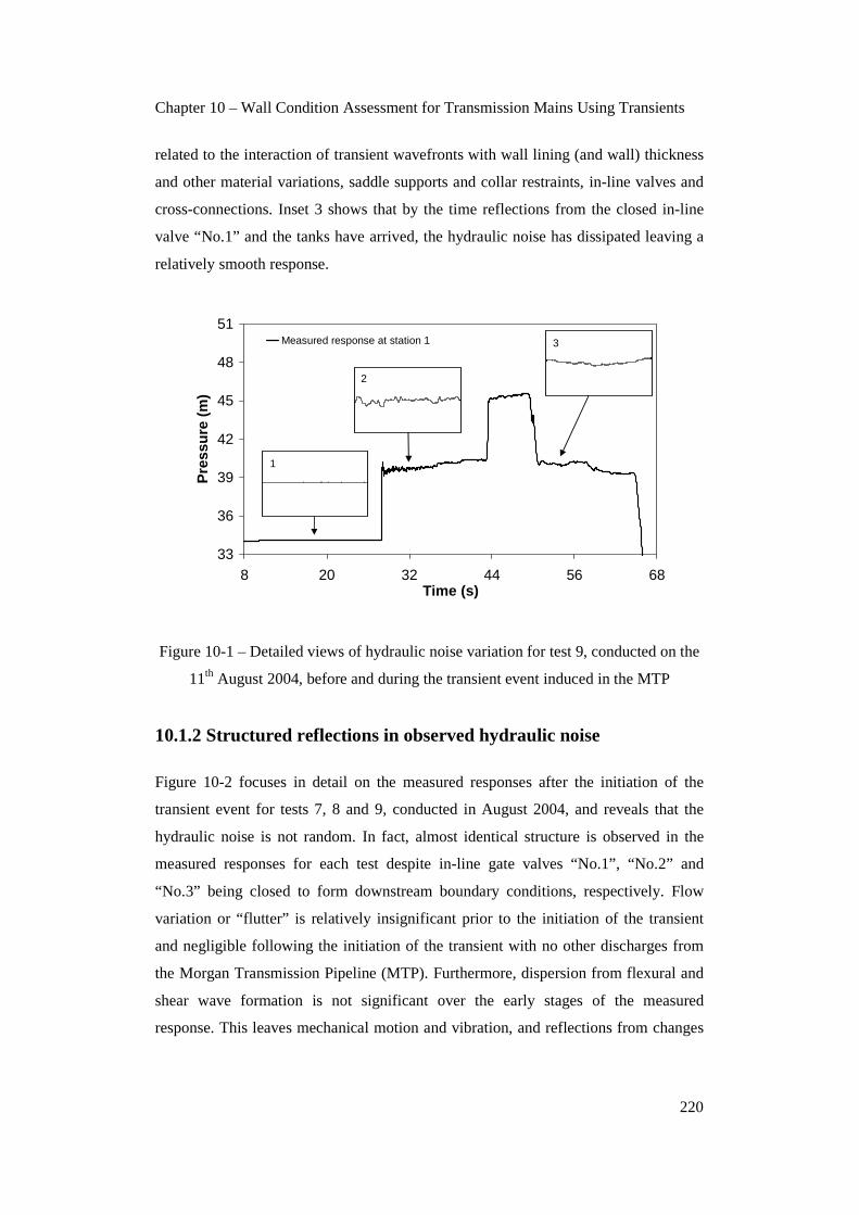
Chapter 10 – Wall Condition Assessment for Transmission Mains Using Transients
220
related to the interaction of transient wavefronts with wall lining (and wall) thickness
and other material variations, saddle supports and collar restraints, in-line valves and
cross-connections. Inset 3 shows that by the time reflections from the closed in-line
valve “No.1” and the tanks have arrived, the hydraulic noise has dissipated leaving a
relatively smooth response.
33
36
39
42
45
48
51
8 20 32 44 56 68Time (s)
Pre
ssu
re (
m)
Measured response at station 1
1
2
3
Figure 10-1 – Detailed views of hydraulic noise variation for test 9, conducted on the
11th August 2004, before and during the transient event induced in the MTP
10.1.2 Structured reflections in observed hydraulic noise
Figure 10-2 focuses in detail on the measured responses after the initiation of the
transient event for tests 7, 8 and 9, conducted in August 2004, and reveals that the
hydraulic noise is not random. In fact, almost identical structure is observed in the
measured responses for each test despite in-line gate valves “No.1”, “No.2” and
“No.3” being closed to form downstream boundary conditions, respectively. Flow
variation or “flutter” is relatively insignificant prior to the initiation of the transient
and negligible following the initiation of the transient with no other discharges from
the Morgan Transmission Pipeline (MTP). Furthermore, dispersion from flexural and
shear wave formation is not significant over the early stages of the measured
response. This leaves mechanical motion and vibration, and reflections from changes

Chapter 10 – Wall Condition Assessment for Transmission Mains Using Transients
221
to the lining and wall thickness along the MTP, as the likely causes of the structured
hydraulic noise observed in the measured responses.
That said, Fluid Structure Interaction (FSI), related to pipeline inertia and precursor
wave formation, does not account for the observed pattern of reflections (as explained
in Chapter 7). This does not preclude other effects from mechanical motion and
vibration and, in particular, flexural wave formation. Indeed, measurements taken
subsequent to the research reported in this thesis, presented by way of example in
Chapter 7, have confirmed inertial effects and structural accelerations and
displacements in lateral (horizontal), vertical and axial directions. However, the
structural oscillations are relatively small and do not contribute to significant
dispersion over the first few seconds of the measured responses. Furthermore, the
structural accelerations and displacements are dispersive and do not generate
reflections in the measured pressure responses.
38.5
38.9
39.3
39.7
40.1
40.5
27.5 27.9 28.3 28.7 29.1 29.5 29.9 30.3
Time (s)
Pre
ssu
re (
m)
Measured response at station 1 - test 7
Measured response at station 1 - test 8
Measured response at station 1 - test 9
Consistent pattern of "structured" reflections
Figure 10-2 – Consistent pattern of structured reflections for tests 7, 8 and 9
conducted on the Morgan Transmission Pipeline in August 2004
10.2 Internal condition of the Morgan Transmission Pipeline
CCTV camera footage of sections of the Morgan Transmission Pipeline (MTP) was
made available by the South Australian Water Corporation and used to determine the
average pipeline roughness over the sections to which the footage relates. The log of

Chapter 10 – Wall Condition Assessment for Transmission Mains Using Transients
222
lining and wall damage, between chainages 15000m and 15400m, is presented below,
and is of particular interest because this section is in close proximity to the location of
the transient generator (chainage 15709m) and measurement station 1 (chainage
15627m) for the tests conducted in August 2004. As a consequence, the measured
response at station 1, including reflections from features within and along the MTP, is
relatively unaffected by dispersion. Figure 10-3 shows the relative positions of the
transient generator, measurement stations 1 and 2, and the surveyed section of the
MTP.
CCTV camera footage was also available for the section of the MTP between
chainage 17200m and chainage 17700m and a log for this section is presented in
Appendix N. Furthermore, CCTV camera investigation was conducted between
chainage 16000m and chainage 16400m. Unfortunately, the South Australian Water
Corporation could not make this footage available at the time of enquiry by the
author. That said, the South Australian Water Corporation officers confirmed that
there was insignificant damage along this section of the MTP.
No. 1No. 2
Gate Valve No.4
Transient source
t=1/4” t=3/16”
t=1/4”
t=3/16”
CH 13231 m CH 15627 mCH 15024 m CH 15709 m
CH 15731 m
CH 15839 m
CH 11740 m
CCTV between CH 15000 m and 15400 m
Figure 10-3 – Close proximity of damaged section of pipeline to transient generator
and measurement station 1
A summary of the damage to the pipeline, as derived from the logs of the CCTV
camera footage between chainages 15000m and 15400m, with the accumulation of

Chapter 10 – Wall Condition Assessment for Transmission Mains Using Transients
223
pieces of cement lining, delamination and the presence of corrosion surmised every
10m, is presented in Table 10-1. At particular locations, a direct estimate of the area
of exposed wall steel was made and a total of 28.3m2 of lining had been lost along the
400m of the MTP surveyed. Figures 10-4 and 10-5 show typical damage to the
cement lining and wall steel along the MTP between chainages 15000m and 15400m.
Figure 10-4 shows delamination and corrosion of exposed steel along a 4m section of
pipeline. Figure 10-5 shows the same section and a collection of pieces of cement
lining in the bottom of the pipeline.
Table 10-1 – Summary of log of CCTV camera investigation for the Morgan
Transmission Pipeline between chainage 15000m and 15400m
Chainage (m)
Damage classification
Exposed steel (m2)
Roughness (mm) Chainage Damage
classification Exposed steel (m2)
Roughness (mm)
15000 Nil 0 1 15210 Nil 0 1
15010 Nil 0 1 15220 P+D 0.1 8
15020 P+D 0.2 8 15230 Nil 0 1
15030 Nil 0 1 15240 Nil 0 1
15040 Nil 0 1 15250 Nil 0 1
15050 Nil 0 1 15260 P+D 0.6 8
15060 Nil 0 1 15270 P+D+R 4.7 8
15070 P+D+R 6.0 8 15280 P+D+R 12.2 8
15080 Nil 0 1 15290 P+R 0.7 8
15090 Nil 0 1 15300 Nil 0 1
15100 P+R 0.1 6 15310 Nil 0 1
15110 P 0 2 15320 Nil 0 1
15120 Nil 0 1 15330 P+D 0.5 8
15130 P 0 2 15340 P+R 0.2 8
15140 Nil 0 1 15350 Nil 0 1
15150 P+R 0.2 8 15360 P+D 0.1 6
15160 P+D+R 0.6 8 15370 Nil 0 1
15170 Nil 0 1 15380 Nil 0 1
15180 P 0 2 15390 P+D 0.6 8
15190 Nil 0 1 15400 P+D+R 1.5 8
15200 Nil 0 1 Average 3.5mm
where P, D and R represent pieces of cement mortar lining (protrusions), delamination of the cement mortar lining and corrosion/rust, respectively

Chapter 10 – Wall Condition Assessment for Transmission Mains Using Transients
224
Figures 10-4 and 10-5 – Delamination and corrosion damage, with accumulated
pieces of cement lining, for the MTP between chainages 15000m and 15400m
10.3 Potential explanations for observed hydraulic noise
10.3.1 Modelling and assessment of discrete air pockets/entrained air
Given the damage to the internal surface of the Morgan Transmission Pipeline (MTP)
identified in the logs of the CCTV camera investigation and rationalised in Table 10-2
(below) to exclude sections where only pieces of cement mortar lining have
accumulated, it was conceivable that discrete air pockets might accumulate at a
number of locations between chainages 15000m and 15400m (and/or between
chainages 17200m and 17700m) along the MTP. The accumulation of such air
pockets was thought to be most likely at locations where the damage included
delaminated lining and/or exposed and corroded steel (as listed in Table 10-2). The
sizes of the discrete air pockets were assumed to be roughly proportional to the level
of observed damage at particular locations.
The discrete air pockets listed in Table 10-2 were included in a forward transient
model of the MTP. Figure 10-6 shows the measured and predicted responses obtained
using a forward transient model without any air pockets and with the distribution of
air pockets described above. The result is predictable and confirms that while the air
pockets give reflections of the correct order of magnitude, the dispersive
characteristics of the air pockets lead to the formation of an amalgam response that is
unrepresentative of the measured response.
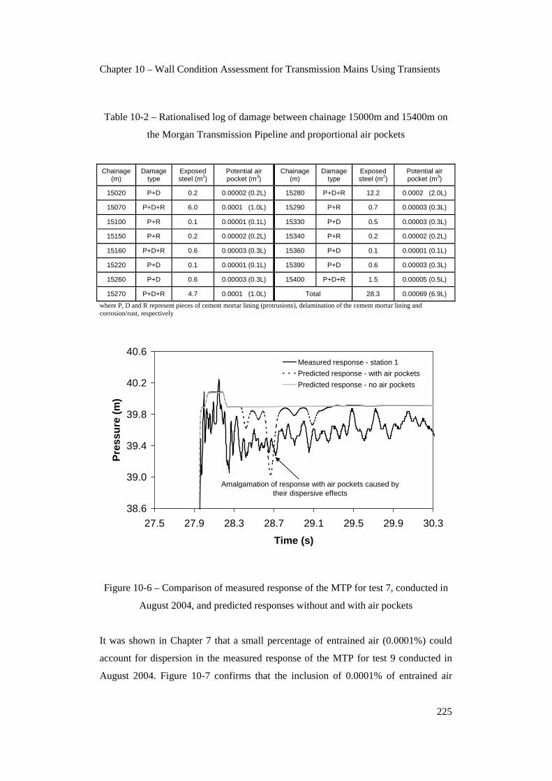
Chapter 10 – Wall Condition Assessment for Transmission Mains Using Transients
225
Table 10-2 – Rationalised log of damage between chainage 15000m and 15400m on
the Morgan Transmission Pipeline and proportional air pockets
Chainage (m)
Damage type
Exposed steel (m2)
Potential air pocket (m3)
Chainage (m)
Damage type
Exposed steel (m2)
Potential air pocket (m3)
15020 P+D 0.2 0.00002 (0.2L) 15280 P+D+R 12.2 0.0002 (2.0L)
15070 P+D+R 6.0 0.0001 (1.0L) 15290 P+R 0.7 0.00003 (0.3L)
15100 P+R 0.1 0.00001 (0.1L) 15330 P+D 0.5 0.00003 (0.3L)
15150 P+R 0.2 0.00002 (0.2L) 15340 P+R 0.2 0.00002 (0.2L)
15160 P+D+R 0.6 0.00003 (0.3L) 15360 P+D 0.1 0.00001 (0.1L)
15220 P+D 0.1 0.00001 (0.1L) 15390 P+D 0.6 0.00003 (0.3L)
15260 P+D 0.6 0.00003 (0.3L) 15400 P+D+R 1.5 0.00005 (0.5L)
15270 P+D+R 4.7 0.0001 (1.0L) Total 28.3 0.00069 (6.9L)
where P, D and R represent pieces of cement mortar lining (protrusions), delamination of the cement mortar lining and corrosion/rust, respectively
38.6
39.0
39.4
39.8
40.2
40.6
27.5 27.9 28.3 28.7 29.1 29.5 29.9 30.3
Time (s)
Pre
ssu
re (
m)
Measured response - station 1
Predicted response - with air pockets
Predicted response - no air pockets
Amalgamation of response with air pockets caused by their dispersive effects
Figure 10-6 – Comparison of measured response of the MTP for test 7, conducted in
August 2004, and predicted responses without and with air pockets
It was shown in Chapter 7 that a small percentage of entrained air (0.0001%) could
account for dispersion in the measured response of the MTP for test 9 conducted in
August 2004. Figure 10-7 confirms that the inclusion of 0.0001% of entrained air

Chapter 10 – Wall Condition Assessment for Transmission Mains Using Transients
226
improves the comparison between the measured and predicted responses in terms of
the initial pressure rise following the induction of the controlled transient. Figure 10-8
confirms that, over the period encompassing the detailed reflections noted above,
0.0001% of entrained air gives a satisfactory match with the timing and slope of the
incident wavefront. Higher percentages of air excessively reduce the initial pressure
rise and overly delay and disperse the predicted wavefront. That said, the inclusion of
0.0001% of entrained air does not account for the observed pattern of reflections.
33
34
35
36
37
38
39
40
41
42
25 27 29 31 33 35
Time (s)
Pre
ssu
re (
m)
Measured response
0.0001%
0.001%
0.01%
33
34
35
36
37
38
39
40
41
42
27.85 27.90 27.95 28.00 28.05 28.10 28.15
Time (s)
Pre
ssu
re (
m)
Measured response
0.0001%
0.001%
0.01%
Figures 10-7 and 10-8 – Effect of different percentages of entrained air, relative to the
measured response for test 7, over time scales of 10s and 0.3s, respectively
10.3.2 Modelling and assessment of minor losses
Misiunas et al. (2005) hypothesised that sections of the Morgan Transmission Pipeline
(MTP) that exhibited higher densities of reflections, with greater magnitudes, when
subject to controlled transient inputs, might have damaged internal linings and walls.
A method was proposed whereby the standard deviation of the measured response for
different 1km long sections of the MTP could be compared to quantitatively gauge
relative levels of damage. The method was not verified against the available CCTV
camera logs because it applied to long lengths of pipeline (greater than or equal to
1km) and could not be used to identify damage with greater specificity. Transient
models incorporating the effects of unsteady friction, discrete and entrained air and
Fluid Structure Interaction (FSI) effects were not developed to assess the potential
impact of these phenomena.
Misiunas (2005) suggested that the mechanism responsible for the observed
reflections was the interaction of the transient wavefront with protrusions, largely

Chapter 10 – Wall Condition Assessment for Transmission Mains Using Transients
227
comprised of delaminated cement lining, from the internal surface of the wall of the
MTP. Based on the CCTV camera logs of the section of the MTP between chainages
15000m and 15400m, the distribution and degree of protrusions from the delaminated
cement lining (and corrosion/tuberculation) has been directly estimated and
summarised in Table 10-3.
Table 10-3 – Log of wall damage and cement lining delamination between chainage
15000m and 15400m on the MTP with corresponding extent of protrusion
Chainage (m) / point
Damage type
Approx. intrusion (m)
Approx. diameter (m)
Chainage (m) / point
Damage type
Approx. intrusion (m)
Approx. diameter (m)
15020 – 1 P+D 0.2 0.53 15260 – 8 P+D 0.1 0.63
15070 – 2 P+D+R 0.3 0.43 15270 P+D+R 0.3 0.43
15100 – 3 P+R 0.2 0.53 15280 P+D+R 0.3 0.43
15110 P 0.3 0.43 15290 P+R 0.1 0.63
15130 – 4 P 0.1 0.63 15330 – 9 P+D 0.1 0.63
15150 – 5 P+R 0.1 0.63 15340 P+R 0.3 0.43
15160 P+D+R 0.2 0.53 15360 – 10 P+D 0.3 0.43
15180 – 6 P 0.2 0.53 15390 – 11 P+D 0.1 0.63
15220 – 7 P+D 0.3 0.43 15400 P+D+R 0.3 0.43
where P, D and R represent pieces of cement mortar lining (protrusions), delamination of the cement mortar lining and
corrosion/rust, respectively
Figure 10-9 illustrates the distribution and degree of protrusion, formed by pieces of
cement lining, listed in Table 10-3 (with chainages corresponding to point labels). The
horizontal scale is distorted to extend from chainage 15000m to 15400m. In contrast
to smaller distribution pipelines with tuberculation, the corrosion and tubercules on
the exposed steel wall surfaces do not form protrusions more than 25mm high. As a
consequence, the bulk of each protrusion comprises loose pieces of cement lining
heaped in piles at the locations shown along the pipeline. These piles of cement lining
should not be represented as an integral change in the internal pipeline diameter over
an extended length. Instead, they are better characterised as a sequence of in-line
orifices or discrete blockages.

Chapter 10 – Wall Condition Assessment for Transmission Mains Using Transients
228
1 2 3 4 5 7 6 8 9 10 11
530mm 630mm 430mm 727.5mm
Figure 10-9 – Distribution and degree of protrusions between chainage 15000m and
15400m along the Morgan Transmission Pipeline
The distribution and extent of the protrusions listed in Table 10-3 were included in a
forward transient model of the MTP as in-line orifices. Figure 10-10 shows the
measured and predicted responses obtained using a forward transient model without
any protrusions and with the distribution of protrusions described above.
38.6
39.0
39.4
39.8
40.2
40.6
27.5 27.9 28.3 28.7 29.1 29.5 29.9 30.3
Time (s)
Pre
ssu
re (
m)
Measured response - station 1
Predicted response - with protrusions
Predicted response - no protrusions
Indistinct reflections from discrete protrusions into pipeline from internal wall surface
Figure 10-10 – Comparison of measured response of MTP for test 7, conducted in
August 2004, and predicted responses without and with discrete protrusions

Chapter 10 – Wall Condition Assessment for Transmission Mains Using Transients
229
The result confirms that direct reflections from protrusions of the magnitude listed in
Table 10-3, and illustrated in Figure 10-9, are not significant. The result can be
confirmed by simple application of the direct equations for reflection and transmission
from a discrete blockage or in-line orifice as presented by Wylie and Streeter (1993)
and summarised in Chapter 3. The behaviour of reflections from discrete blockages,
equivalent to the protrusions illustrated in Figure 10-9, is further investigated in
Chapter 13 in the context of field tests on a water distribution pipeline. The analysis
presented in Chapter 13 and, in particular, Appendix S identifies the percent
constrictions required to create discernable reflections from discrete constrictions or
protrusions. None of the protrusions identified in the CCTV camera investigation of
the MTP are of a sufficient extent so as to give rise to the reflections observed in the
measured response.
10.4 Correlating internal pipe condition with reflections
The observation by Misiunas et al. (2005), that there is a correlation between damage
to the inside of the wall of the Morgan Transmission Pipeline (MTP) and the density
and magnitude of reflections observed from 1km long sections of the pipeline subject
to transient tests (i.e., the standard deviation of the pressure response), is thought to be
correct. However, it has been necessary to develop complex forward transient models
of the MTP in order to assess the potential impact of lateral pipes, cross-connections,
discrete air pockets, entrained air and fluid structure interaction effects (as far as they
relate to inertial effects). Furthermore, the mechanism identified by Misiunas (2005),
which suggests that there are reflections from the deposits of internal lining that have
built-up along the bottom of the MTP, is contradicted by the results of transient
modelling and the application of the direct equations for reflection and transmission
presented by Wylie and Streeter (1993).
Given the systematic elimination of other plausible explanations, and the fact that the
reflections occur with the same magnitude and distribution for repeated tests
(suggesting that they are related to the invariant (or very slowly varying) physical
characteristics of the MTP), it is postulated that the reflections are correlated with
changes in the wave speed of the MTP at locations at which there has been

Chapter 10 – Wall Condition Assessment for Transmission Mains Using Transients
230
delamination of the cement lining around the internal circumference of the pipeline
and where wall corrosion has occurred.
10.4.1 Theoretical effect of changes to lining and wall thickness
The wave speed for the sections of the Morgan Transmission Pipeline (MTP) with
3/16 of an inch (4.76mm) thick wall is theoretically 1015m/s when the pipeline is
taken to be fully restrained. This wave speed was determined assuming composite
action between the steel wall and cement lining with the physical and geometric
properties shown in Figure 10-11. If in good condition, nearly all of the pipeline in
close proximity to the location of the transient generator and measurement station 1,
for tests 7, 8 and 9, conducted in August 2004, has a 4.76mm thick wall. However,
there is a relatively short section of pipeline with a 1/4 of an inch (6.35mm) thick wall
between chainage 15731m and chainage 15839m as shown in Figure 10-3 (above).
The wave speed for the section of pipeline with this wall thickness is theoretically
1074m/s.
727.5 mm
762 mm
tS = 4.76 mm
MSCL pipeline in good condition with intact cement lining and no wall corrosion
Wave speed a = 1015 m/s
tC = 12.5 mm
Figure 10-11 – Morgan Transmission Pipeline in good condition with intact cement
lining
The transient response of the MTP is extremely sensitive to the wave speed, which is,
in turn, sensitive to the condition of the pipeline wall. If we recall the traditional

Chapter 10 – Wall Condition Assessment for Transmission Mains Using Transients
231
Method of Characteristics (MOC) solution for the C+ and C- compatibility equations
along the characteristic lines of the MOC grid, with a quasi-steady representation of
friction, then the solution for the transient pressure can be obtained using:
( ) ( ) ( )
( ) ( )+
+
⎥⎦
⎤⎢⎣
⎡∆−∆−∆+
−⎥⎦
⎤⎢⎣
⎡∆−∆−+∆−∆−=
txQttxxQtagDA
f
gA
a
ttxxQgA
attxxHtxH
,,2
,,,
2
(10-1)
and
( ) ( ) ( )
( ) ( )−
−
⎥⎦
⎤⎢⎣
⎡∆−∆+∆+
+⎥⎦
⎤⎢⎣
⎡∆−∆+−∆−∆+=
txQttxxQtagDA
f
gA
a
ttxxQgA
attxxHtxH
,,2
,,,
2
(10-2)
where f is a steady state friction factor, a is the wave speed, A is the internal area of
the pipeline and the impedance of the pipeline gA
aB =
It is apparent, through the impedance term, that the transient response of the pipeline
is sensitive to the wave speed and the internal area of the pipeline. The loss of the
cement lining reduces the stiffness of the pipeline wall by an amount proportional to
the thickness and modulus of elasticity of the cement. Once exposed, the pipe wall
begins to corrode leading to a reduction in the thickness of the metal retaining its
original elastic modulus. If the pipeline wall is damaged, and has lost cement lining
and/or developed wall corrosion, the wave speed will decrease, and the internal area
of the pipeline will increase, such that there will be a reduction of pipeline impedance.
As the variability in the condition of the pipeline wall increases so too does the
magnitude and density of reflections following the passage of a sharp transient
wavefront. As a consequence, it may be possible to replicate the effect of a damaged
section of pipeline by varying its physical and geometric properties along its length.

Chapter 10 – Wall Condition Assessment for Transmission Mains Using Transients
232
Based on examination of the CCTV camera footage for the sections of the MTP
between chainage 15000m and chainage 15400m, and also chainage 17200m and
17700m, it was decided to characterise the damage to the internal surface of the walls
of the MTP in terms of four discrete categories of damage. While individual pits (i.e.,
points of specific corrosion) could not be represented, the loss of cement lining could
be specified, as could average reductions in pipeline wall thickness for different
degrees of corrosion. Table 10-4 summarises the four categories of damage, the
change to internal pipe diameter, the status of the cement lining, thickness of steel that
has corroded and, finally, the wave speed corresponding to each level of damage. The
wave speed is a function of the change to internal pipe diameter and remaining
thickness of cement lining and steel in the pipeline wall and has been calculated using
the relationship presented by Wylie and Streeter (1993) and described in Appendix S.
Table 10-4 – Physical and geometric properties of the Morgan Transmission Pipeline
for four discrete levels of damage
Level of Damage
Description of Damage
Internal Diameter
(mm)
Cement Lining
Corroded Metal
Thickness (mm)
Un-corroded Metal
Thickness (mm)
Wave Speed (m/s)
0 Nil 727.5 Intact 0 4.76 1015
1 Loss of cement lining
752.5 None 0 4.76 932
2 1mm of corrosion 754.5 None 1 3.76 865
3 2mm of corrosion 756.5 None 2 2.76 778
4 3mm of corrosion 758.5 None 3 1.76 655
Figure 10-12 shows the idealised physical characteristics of the MTP for the four
discrete levels of damage that include the pipeline without cement lining and with
0mm, 1mm, 2mm and 3mm of wall corrosion, respectively.

Chapter 10 – Wall Condition Assessment for Transmission Mains Using Transients
233
752.5 mm
762 mm
tS = 4.76 mm
MSCL pipeline without cement lining but no wall corrosion
Wave speed a = 932 m/s
762 mm
tS = 3.76 mm
MSCL pipeline without cement lining and 1mm average wall corrosion
Wave speed a = 865 m/s
754.5 mm
762 mm
tS = 2.76 mm
MSCL pipeline without cement lining and 2mm average wall corrosion
Wave speed a = 778 m/s
756.5 mm
762 mm
tS = 1.76 mm
MSCL pipeline without cement lining and 3mm average wall corrosion
Wave speed a = 655 m/s
758.5 mm
Figure 10-12 – Four discrete levels of pipe wall damage for the Morgan Transmission
Pipeline
10.4.2 Representing the effects of known damage and wall changes
Table 10-5 summarises the condition of the Morgan Transmission Pipeline (MTP), in
terms of the categories of damage identified above over 10m lengths of pipeline,
between chainage 15000m and chainage 15400m. Loss of cement lining without
significant corrosion was observed, on average, over the 10m lengths of pipeline
centred on chainages 15020m, 15110m and 15180m. For all other damaged sections,
the loss of cement lining was accompanied by various degrees of corrosion of the
internal pipeline wall.
Figure 10-13 shows the effect of the known change in wall thickness between
chainage 15731m and 15839m from 4.76mm to 6.35mm, and back to 4.76mm, and
the distribution and extent of categorised damage, estimated using the CCTV camera
footage, between chainage 15000m and 15400m, upon the wave speed of the MTP.

Chapter 10 – Wall Condition Assessment for Transmission Mains Using Transients
234
Table 10-5 – Approximate known condition of the MTP, in terms of diameter and
wave speed, per 10m length, between chainage 15000m and 15400m
Chainage (m)
Damage Level
Internal Diameter
(m)
Wave Speed (m/s)
Chainage (m)
Damage Level
Internal Diameter
(m)
Wave Speed (m/s)
15000 Nil 0.7275 1015 15210 Nil 0.7275 1015 15010 Nil 0.7275 1015 15220 2 0.7545 865 15020 1 0.7525 932 15230 Nil 0.7275 1015 15030 Nil 0.7275 1015 15240 Nil 0.7275 1015 15040 Nil 0.7275 1015 15250 Nil 0.7275 1015 15050 Nil 0.7275 1015 15260 2 0.7545 865 15060 Nil 0.7275 1015 15270 3 0.7565 778 15070 3 0.7565 778 15280 3 0.7565 778 15080 Nil 0.7275 1015 15290 2 0.7545 865 15090 Nil 0.7275 1015 15300 Nil 0.7275 1015 15100 2 0.7545 865 15310 Nil 0.7275 1015 15110 1 0.7525 932 15320 Nil 0.7275 1015 15120 Nil 0.7275 1015 15330 3 0.7565 778 15130 Nil 0.7275 1015 15340 2 0.7545 865 15140 Nil 0.7275 1015 15350 Nil 0.7275 1015 15150 2 0.7545 865 15360 2 0.7545 865 15160 3 0.7565 778 15370 Nil 0.7275 1015 15170 Nil 0.7275 1015 15380 Nil 0.7275 1015 15180 1 0.7525 932 15390 3 0.7565 778 15190 Nil 0.7275 1015 15400 3 0.7565 778 15200 Nil 0.7275 1015
500
600
700
800
900
1000
1100
1200
14300
14400
14500
14600
14700
14800
14900
15000
15100
15200
15300
15400
15500
15600
15700
15800
15900
16000
Chainage (m)
Wav
e sp
eed
(m
/s)
Extent of CCTV camera footage
Deteriorated cement lining / corrosion
Change in wall thickness from 4.76mm to 6.35mm
Figure 10-13 – Distribution and extent of changes to the MTP wave speed, estimated
over 10m lengths, between chainage 15000m and 15400m

Chapter 10 – Wall Condition Assessment for Transmission Mains Using Transients
235
10.4.3 Transient modelling of known wall changes
Although Equations 10-1 and 10-2 presented above represent a traditional transient
solution scheme with quasi-steady friction, the forward transient model developed for
the following analysis includes turbulent rough pipe unsteady friction, using the
roughness values determined on the basis of the CCTV camera footage, and 0.0001%
of entrained air (as previously determined in Chapter 7 as the most realistic quantity).
“Viscous” damping mechanisms have not been included in the forward transient
model. A 10m discretisation, and hence 10m resolution for the classification of
damaged sections of the Morgan Transmission Pipeline (MTP), has been adopted.
This length matches that over which the average condition of the MTP was
catergorised using the CCTV camera footage. A 5m discretisation has also been used,
to assess the sensitivity of the modelled response to discretisation and interpolation
errors, below.
Apart from the estimated changes to the wall of the MTP between chainage 15000m
and 15400m, it was known that the pipeline wall thickness changed between chainage
15731m and 15839m from 4.76mm to 6.35mm, and back to 4.76mm, and that it
changed from 4.76mm to 6.35mm at chainage 11740m. Figure 10-14 shows the
comparison between the measured (test 7) and predicted responses, at station 1, when
these known changes in the wall thickness are included, as well as the known damage
inferred from the CCTV camera footage between chainage 15000m and 15400m.
Unfortunately, the effects of the change in thickness between chainage 15731m and
chainage 15839m are partially obscured by the incident wavefront because of its close
proximity to the transient generator and station 1. That said, the additional reflections
(positive and negative) associated with the changes in wall thickness are apparent and
have a magnitude of approximately 0.16m.
The reflection from the change in pipeline wall thickness at chainage 11740m is
clearly discernable and is also approximately 0.16m in magnitude. The measured and
predicted magnitude of the reflection, and the timing, compare favourably. The results
confirm that reflections from changes in pipe wall thickness from 4.76mm to 6.35mm
(i.e., 25%) are observed in the measured response and can be predicted using the
forward transient model. Furthermore, this magnitude of change in pipe wall thickness

Chapter 10 – Wall Condition Assessment for Transmission Mains Using Transients
236
is comparable with that for the damage categories identified above. The discrepancy
between the measured and predicted transient plateau, once the limits of the known
information regarding the damage to the pipe wall are reached, appears to be related
to the neglect of further damage along the pipeline that has not been included in the
forward transient model. Similarly, the lag between the predicted and measured
reflection is likely to be related to an unaccounted for reduction in the wave speed
along damaged sections of pipeline.
38.0
38.5
39.0
39.5
40.0
40.5
41.0
41.5
26 28 30 32 34 36 38
Time (s)
Pre
ssu
re (
m)
Measured response - station 1
Predicted response - no damage
Predicted response - with damage
Effect of change in wall thickness at chainages 15731m and 15839m
Effect of "known" damage
Damage effecting response along "plateau" is unknown
Effect of change in wall thickness at chainage 11740m
Figure 10-14 – Measured and predicted responses when known changes in wall
thickness and known damage are included in a forward transient model of the MTP
10.4.4 Inferring the condition of a section of the MTP
Figure 10-15 shows the measured (test 7) and predicted responses when known
damage, between chainage 15000m and chainage 15400m, is included in the forward
transient model. The validity of the comparison is restricted, to between times 28.35s
and 29.20s, because the range over which the lining and wall condition are known is
limited to the extent of the CCTV camera footage. Within this range, trends in the
predicted response approximately match those in the measured response.

Chapter 10 – Wall Condition Assessment for Transmission Mains Using Transients
237
38.6
39.0
39.4
39.8
40.2
40.6
27.5 27.9 28.3 28.7 29.1 29.5 29.9 30.3
Time (s)
Pre
ssu
re (
m)
Measured response - station 1
Predicted response - no damage
Predicted response - with 'known' damage
Limit of valid comparison
Figure 10-15 – Measured and predicted responses when known damage between
chainage 15000m and 15400m is included in the forward transient model
Discrepancies are likely to be due to the categorisation process by which the damage
is included in the forward transient model and differences between the damage
inferred from the CCTV footage and the actual physical condition of the pipe wall.
However, the important point is that the inclusion of the idealised damage, at
locations that were physically confirmed using the CCTV camera footage, has led to a
significant improvement in the comparison between the measured and predicted
responses. Neither the inclusion of entrained air pockets nor discrete protrusions in the
forward transient model gave this improvement.
An inferred distribution of damage has been determined for the remainder of the MTP
between chainage 14300m and 16000m. Figure 10-16 shows the inferred pattern of
damage, in terms of changes in wave speed, combined with the known damage,
between chainage 14300m and 16000m. South Australian Water Corporation officers
provided advice that there was insignificant damage to the MTP between chainage
16000m and 16400m. This has been relied upon when determining the inferred
distribution of damage.

Chapter 10 – Wall Condition Assessment for Transmission Mains Using Transients
238
500
600
700
800
900
1000
1100
1200
14300
14400
14500
14600
14700
14800
14900
15000
15100
15200
15300
15400
15500
15600
15700
15800
15900
16000
Chainage (m)
Wav
e sp
eed
(m
/s)
Deteriorated cement lining / corrosion
Change in wall thickness from 4.76mm to 6.35mm
Known condition Inferred conditionInferred condition
Figure 10-16 – Inferred and known distribution and extent of changes to the MTP
wave speed, estimated over 10m lengths, between chainage 14300m and 16000m
Figure 10-17 shows that this combined distribution of inferred and known damage
improves the comparison between the measured and predicted responses (over the full
range between times 27.9s and 30.3s). It appears the changes in the wall condition,
and corresponding changes in wave speed and impedance, provide an explanation for
the observed reflections and, potentially, a way of inferring the damage to the pipeline
wall by interpreting reflections using a forward transient model when known
information is not available.
That said, the inferred distribution of damage has been determined by limited trial and
error analysis and is not an optimal representation of the likely damage to the pipeline
wall. This explains, in part, the discrepancies between the measured and predicted
responses and represents a further complication additional to those introduced by the
categorisation of the damage and the use of a 10m discretisation in the forward
transient model.
Apart from suggesting that dispersion due to entrained air and/or mechanical
dispersion and damping is not significant over the initial stages of the response, the
density of reflection detail in the measured responses suggests that variations in
damage to the pipe wall are significant on a metre for metre basis. The use of a finer

Chapter 10 – Wall Condition Assessment for Transmission Mains Using Transients
239
discretisation in the forward transient model is feasible and would increase the
specificity with which known or inferred damage, could be represented. Figure 10-18
shows the predicted response obtained for a forward transient model with a 5m
discretisation.
38.6
39.0
39.4
39.8
40.2
40.6
27.5 27.9 28.3 28.7 29.1 29.5 29.9 30.3
Time (s)
Pre
ssu
re (
m)
Measured response - station 1
Predicted response - no damage
Predicted response - 'known' + inferred damage
Figure 10-17 – Measured and predicted responses with known and inferred damage in
a forward transient model with a 10m discretisation
38.6
39.0
39.4
39.8
40.2
40.6
27.5 27.9 28.3 28.7 29.1 29.5 29.9 30.3
Time (s)
Pre
ssu
re (
m)
Measured response - station 1
Predicted response - 10m discretisation
Predicted response - 5m discretisation
Figure 10-18 – Measured and predicted responses with known and inferred damage in
a forward transient model with 10m and 5m discretisations, respectively

Chapter 10 – Wall Condition Assessment for Transmission Mains Using Transients
240
10.4.5 Use of evolutionary algorithm for inferring pattern of damage
The intention in this chapter has been to identify a physical mechanism that can
explain the observed reflections and explore the possibility that a forward transient
model could be applied to both confirm the effect of a known distribution of damage
and predicatively infer a distribution of damage from a measured response. The
inferred distribution of damage presented above has been determined on the basis of
limited trial and error variation of the magnitude and distribution of damage and does
not represent the optimal inferred distribution that gives the best match between the
measured and predicted responses.
The use of trial and error analysis cannot be relied upon in future investigation of the
methodology because of the number of potential combinations of damage magnitudes
and distributions over even relatively short sections of pipeline. In the case of the
Morgan Transmission Pipeline (MTP), between chainage 14300m and 16000m, there
are 170 by 10m long sections that can each have one of 5 conditions (i.e., either
undamaged or category 1, 2, 3 or 4). This gives an extremely large number of possible
combinations of magnitude and distribution of damage.
The application of global optimisation algorithms is required to determine the
distribution of damage that gives the optimal fit between the measured and predicted
responses. In this regard, either a Genetic Algorithm, or the Shuffled Complex
Evolution Algorithm used in the inverse analysis presented in this research, may be
used to fit for discrete levels of damage at 10m (or other) intervals along a section of
pipeline. At the time of writing, the author has completed the programming work
required to combine a Genetic Algorithm with the forward transient model
BSOLVER (previously described).
10.4.6 Numerical exploration of operation of evolutionary algorithm
Unfortunately, for the tests conducted on the Morgan Transmission Pipeline (MTP) in
August 2004, measurement station 2 is not close enough to the damaged section of
pipeline between chainage 15000m and 15400m, or the transient generator and station

Chapter 10 – Wall Condition Assessment for Transmission Mains Using Transients
241
1, to enable the measured response at station 2 to be used as input for the program
combining the Genetic Algorithm and forward transient model. This is because the
reflections measured at this station are significantly dispersed and the transient model
required to include measurement stations 1 and 2, and the transient generator, with a
discretisation of 10m, requires too many sub-pipe sections (nearly 500).
That said, issues can be numerically explored and the operation of the combined
Genetic Algorithm and BSOLVER developed in this research can be demonstrated.
This will be done using a 1000m long numerical pipe example and then a 1500m long
representation of the MTP encompassing the location near SC22, AV39 and AV41.
The pattern of damage along the 1500m pipeline will be a composite of the known
damage identified using the CCTV camera footage, the damage inferred from the trial
and error analysis described above and an artificial pattern for the remainder of the
pipeline.
Description of numerical pipeline and results of inverse analysis
Figure 10-19 shows the 1000m long numerical pipeline example. The pipeline
diameter is 727.5mm (i.e., the same as for the Morgan Transmission Pipeline (MTP)).
However, the pipeline is treated as frictionless with a roughness of 0mm.
Furthermore, the pipeline is at the same relative elevation along its entire length. An
assumed reservoir depth of 40m is applied to give similar static pressures to those
observed in the MTP at the location of scour valve 22. As for test 7, conducted on the
MTP in August 2004, the pressure response is determined at three locations (namely,
measurement stations 1 and 2 and at the transient generator). These locations are
250m, 500m and 750m from the closed valve, respectively.
Four categories of damage are used to simulate the deterioration of the wall of the
MTP over 10m lengths as described above. The loss of cement mortar lining (CML)
without corrosion of the steel pipeline wall is category 1, and categories 2, 3 and 4
have lost CML and 1mm, 2mm and 3mm of corroded wall thickness, respectively.
The different categories of damage are shown in Figure 10-19 at seven arbitrary
locations selected for the purpose of this example. Each damaged section of pipeline
is 10m long.

Chapter 10 – Wall Condition Assessment for Transmission Mains Using Transients
242
G QSIDE DISCHARGE
HR = 40m
QV = 0 L/s
ε= 0.0mm (frictionless)
M1 M2
750m
500m
250m
1000m
Pipe segment – 89 Damage level – 3
Pipe segment – 13 Damage level – 2
Pipe segment – 83 Damage level – 1
Pipe segment – 39 Damage level – 3
Pipe segment – 69 Damage level – 1
Pipe segment – 57 Damage level – 2
Pipe segment – 31 Damage level – 4
D= 727.5mm
M1 = measurement station 1 M2 = measurement station 2 G = generator measurement station
Damage level Internal diameter (mm)
Wave speed (m/s)
Remaining wall thickness (mm)
Comment
0 727.5 1015 100% Undamaged
1 752.5 932 100% No CML + no corrosion
2 754.5 865 79% No CML + 1mm corrosion
3 756.5 778 58% No CML + 2mm corrosion
4 758.5 655 37% No CML + 3mm corrosion
9 8 7 6 5 4 3 2 1 100 99 98 97
Figure 10-19 – Example pipeline used to numerically test the inverse transient model
for wall condition assessment using a Genetic Algorithm and BSOLVER
Figure 10-20 shows the pattern of damage along the numerical pipeline, represented
in terms of reduction in wave speed and loss of CML and/or corrosion of wall
thickness, artificially established for this example, and the pattern of damage
predicted after performing inverse analysis. Forward transient responses were
determined for the numerical example using BSOLVER and these were used as
artificial measurements when performing the inverse analysis using NLFIT,
BSOLVER and a Genetic Algorithm.
The inverse analysis was performed with 64 (i.e., 26) divisions of the potential values
for wave speed, between bounds of 655m/s and 1015m/s, for each 10m sub-pipe
segment (i.e., one of 64 uniformly distributed wave speeds, increasing in 5.625m/s
increments from 655m/s to 1015m/s, could be fitted for each sub-pipe length). This
number of divisions was selected after performing sensitivity checks to determine the
balance between the number of potential wave speed values between the bounds, and
the resultant improvement in accuracy of fit, and the size of the inverse search space
which increased with the number of wave speed values. Further investigation of the
optimum number of divisions is continuing outside the scope of this research.

Chapter 10 – Wall Condition Assessment for Transmission Mains Using Transients
243
The lower and upper bounds were determined using the minimum and maximum
wave speeds that could feasibly give rise to the observed pattern of reflections (i.e.,
the magnitude of the lowest reflection was such that a wave speed of less than 655m/s
in any one sub-pipe segment was not feasible). This result follows from the fact that
the lowest artificial wave speed for the numerical example was 655m/s. The
importance of bounding the search space is investigated further below. In the case of a
field pipeline, the lower bound can be determined, before conducting inverse analysis,
by examining the measured responses and identifying the lowest feasible wave speed
over a 10m length of pipe that can give rise to the observed reflections.
650
700
750
800
850
900
950
1000
1050
0 250 500 750 1000
Chainage (m)
Wav
e S
pee
d (
m/s
)
Damage level 1 Damage level 2
Damage level 3 Damage level 4
Wave Speed (m/s) Measurement Points
655m/s to 1015m/s bounds
M1 M2G
Location at which transient is generated
79%
Approximate % of remaining wall thickness
58%
100%
37%
100%
no CML
Figure 10-20 – Artificial pattern of damage versus fitted pattern of damage, in terms
of wave speed and wall thickness reduction, for the numerical pipeline example
The artificial and fitted patterns of damage match closely after approximately 500000
evaluations using BSOLVER. Figure 10-21 shows the improvement in the objective
function for the inverse fitting over the first 50000 evaluations. Most of the
improvement in the fit occurs over the first 50000 of the 500000 evaluations. The
discrepancies between the patterns of damage are problematic given the fitted damage
was determined using the same forward transient response data in BSOLVER during
the inverse analysis. Investigation into this discrepancy is continuing and it is

Chapter 10 – Wall Condition Assessment for Transmission Mains Using Transients
244
suspected to be partly related to the large number of parameters being fitted (i.e., 100
parameters).
0 10000 20000 30000 40000 50000Evaluations
0.0
30.0
60.0
90.0
120.0
150.0
Obj function
Figure 10-21 – Improvement in objective function over first 50000 evaluations using
NLFIT, BSOLVER and a Genetic Algorithm
Figure 10-22 shows that the artificial numerical response and the response determined
after fitting are similar at the location of the transient generator. This is despite the
discrepancies between the artificial and fitted patterns of damage noted above. Figures
10-23 and 10-24 show that the artificial numerical responses and those determined
after fitting are also similar at measurement locations 1 and 2. This indicates a loss of
sensitivity in the inverse analysis as the weaker reflections are replicated and may
help explain the residual discrepancies between the artificial and fitted patterns of
damage. It is evident that approximately 0.45s passes before the wavefronts reach
stations 1 and 2 and that there is less transient information available at these locations
than at the transient generator. The inverse analysis is limited to 0.9s to avoid
reflections from the artificial closed valve and reservoir boundary conditions
influencing the results.

Chapter 10 – Wall Condition Assessment for Transmission Mains Using Transients
245
39.0
40.0
41.0
42.0
43.0
44.0
45.0
46.0
47.0
0.0 0.1 0.2 0.3 0.4 0.5 0.6 0.7 0.8 0.9Time (s)
Pre
ssu
re (
m)
Measured "artificial" response
Predicted "fitted" response
Figure 10-22 – Artificial and fitted transient responses at the transient generator
39.0
40.0
41.0
42.0
43.0
44.0
45.0
46.0
47.0
0.0 0.1 0.2 0.3 0.4 0.5 0.6 0.7 0.8 0.9
Time (s)
Pre
ssu
re (
m)
Measured "artificial" response
Predicted "fitted" response
39.0
40.0
41.0
42.0
43.0
44.0
45.0
46.0
47.0
0.0 0.1 0.2 0.3 0.4 0.5 0.6 0.7 0.8 0.9
Time (s)
Pre
ssu
re (
m)
Measured "artificial" response
Predicted "fitted" response
Figure 10-23 and 10-24 – Artificial and fitted transient responses at measurement
locations 1 and 2, respectively
Search space issues
The larger the search space for the inverse problem the more difficult it is to identify
parameters that give the best fit between measured and predicted responses. As
mentioned above, increasing the number of divisions between the wave speed bounds
increases the search space for the inverse problem. However, it also increases the
accuracy with which a unique wave speed can be identified. The Genetic Algorithm in
NLFIT is discrete (i.e., searches for discrete rather continuous parameter values).
However, the search space between the wave speed bounds can be divided into binary

Chapter 10 – Wall Condition Assessment for Transmission Mains Using Transients
246
multiples of 22, 23, 24, 25, 26, 27, 28, 29 up to 212. That is, the search space can be
divided into 4, 8, 16, 32, 64, 128, 256, 512 up to 4096 wave speeds such that the
available values trend from 4 discrete values to 4096 finely spaced semi-continuous
values, respectively. In the case of 4 divisions, the available wave speeds are 655,
775, 895 and 1015m/s. These values are reasonably close to the categories established
earlier with wave speeds of 655, 778, 865, 932 and 1015m/s, respectively. Further
division of the available values gives more flexibility to fit parameters closer to the
arbitrary categories (i.e., for 4096 divisions the available wave speeds increase from
655m/s in 0.0879m/s increments such that 778, 865 and 932m/s are available).
However, this additional division increases the size of the search space such that
optimum solutions are not achieved. Sensitivity analysis has revealed that, for the
numerical problem posed in this section, approximately 64 divisions gives the
smallest relative objective function and this number of divisions will be used for the
remainder of the analysis.
It was also mentioned above that the lower and upper bounds can be determined using
the minimum and maximum wave speeds that feasibly give rise to the observed
pattern of reflections. Figure 10-25 compares the results of the inverse analysis when
lower bounds of 655m/s and 500m/s are used.
650
700
750
800
850
900
950
1000
1050
0 250 500 750 1000
Chainage (m)
Wav
e S
pee
d (
m/s
)
Damage level 1 Damage level 2
Damage level 3 Damage level 4
Wave Speed (m/s) Measurement Points
655m/s lower bound 500m/s lower bound
M1 M2G
Location at which transient is generated
79%
Approximate % of remaining wall thickness
58%
100%
37%
100%
no CML
Figure 10-25 – Effect of reducing lower bound from 655m/s to 500m/s and increasing
the inverse search space
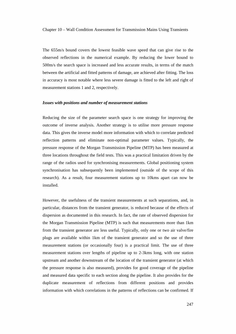
Chapter 10 – Wall Condition Assessment for Transmission Mains Using Transients
247
The 655m/s bound covers the lowest feasible wave speed that can give rise to the
observed reflections in the numerical example. By reducing the lower bound to
500m/s the search space is increased and less accurate results, in terms of the match
between the artificial and fitted patterns of damage, are achieved after fitting. The loss
in accuracy is most notable where less severe damage is fitted to the left and right of
measurement stations 1 and 2, respectively.
Issues with positions and number of measurement stations
Reducing the size of the parameter search space is one strategy for improving the
outcome of inverse analysis. Another strategy is to utilise more pressure response
data. This gives the inverse model more information with which to correlate predicted
reflection patterns and eliminate non-optimal parameter values. Typically, the
pressure response of the Morgan Transmission Pipeline (MTP) has been measured at
three locations throughout the field tests. This was a practical limitation driven by the
range of the radios used for synchronising measurements. Global positioning system
synchronisation has subsequently been implemented (outside of the scope of this
research). As a result, four measurement stations up to 10kms apart can now be
installed.
However, the usefulness of the transient measurements at such separations, and, in
particular, distances from the transient generator, is reduced because of the effects of
dispersion as documented in this research. In fact, the rate of observed dispersion for
the Morgan Transmission Pipeline (MTP) is such that measurements more than 1km
from the transient generator are less useful. Typically, only one or two air valve/fire
plugs are available within 1km of the transient generator and so the use of three
measurement stations (or occasionally four) is a practical limit. The use of three
measurement stations over lengths of pipeline up to 2-3kms long, with one station
upstream and another downstream of the location of the transient generator (at which
the pressure response is also measured), provides for good coverage of the pipeline
and measured data specific to each section along the pipeline. It also provides for the
duplicate measurement of reflections from different positions and provides
information with which correlations in the patterns of reflections can be confirmed. If

Chapter 10 – Wall Condition Assessment for Transmission Mains Using Transients
248
less than three measurements are taken, then the loss of information along the
adjacent section of pipeline is significant. Figure 10-26 shows the effect of removing
the measured response at the transient generator for the numerical pipeline example.
Damage is erroneously predicted between measurement stations M1 and M2 (i.e., in
the region where the transient generator measurement has been removed).
650
700
750
800
850
900
950
1000
1050
0 250 500 750 1000
Chainage (m)
Wav
e S
pee
d (
m/s
)
Damage level 1 Damage level 2
Damage level 3 Damage level 4
Wave Speed (m/s) Measurement Points
G+M1+M2 M1+M2
M1 M2G
Location at which transient is generated
79%
Approximate % of remaining wall thickness
58%
100%
37%
100%
no CML
Figure 10-26 – Effect of removing measured response at the transient generator upon
the results of the inverse analysis
Figures 10-27 and 10-28 show the effect of removing the measured response at
stations M1 and M2, respectively. Erroneous damage is predicted in the region of the
pipeline adjacent to measurement station M1 when it is removed from the inverse
analysis. Similarly, erroneous damage is predicted in the region of the pipeline
adjacent to measurement station M2 when it is removed. The extent of the erroneous
damage is greater when M2 is removed. This is because the majority of the artificial
damage is on the M1 side of the transient generator and the reflections that were
recorded at M2 provided important information regarding this region of the pipeline.
The results confirm that it is important to cover the length of pipeline under
investigation with as many measurement locations as practical.

Chapter 10 – Wall Condition Assessment for Transmission Mains Using Transients
249
650
700
750
800
850
900
950
1000
1050
0 250 500 750 1000
Chainage (m)
Wav
e S
pee
d (
m/s
)
Damage level 1 Damage level 2
Damage level 3 Damage level 4
Wave Speed (m/s) Measurement Points
G+M1+M2 G+M2
M1 M2G
Location at which transient is generated
79%
Approximate % of remaining wall thickness
58%
100%
37%
100%
no CML
650
700
750
800
850
900
950
1000
1050
0 250 500 750 1000
Chainage (m)
Wav
e S
pee
d (
m/s
)
Damage level 1 Damage level 2
Damage level 3 Damage level 4
Wave Speed (m/s) Measurement Points
G+M1+M2 G+M1
M1 M2G
Location at which transient is generated
79%
Approximate % of remaining wall thickness
58%
100%
37%
100%
no CML
Figure 10-27 and 10-28 – Effect on the results of the inverse analysis of removing the
measured responses at M1 and M2, respectively
Another issue is the location of the measurement stations relative to the source of the
transient (i.e., the location of the transient generator). For the numerical example
presented above M1, G and M2 are located at 250, 500 and 750m from the closed in-
line valve boundary condition. Figure 10-29 shows the effect of moving M1 and M2
such that M1, G and M2 are located at 350, 500 and 650m from the closed in-line
valve boundary condition. The comparison between the artificial and fitted damage
patterns is improved between measurement stations M1 and M2, in the region of the
transient generator, because more information is concentrated along this section of the
pipeline.
650
700
750
800
850
900
950
1000
1050
0 250 500 750 1000
Chainage (m)
Wav
e S
pee
d (
m/s
)
Damage level 1 Damage level 2
Damage level 3 Damage level 4
Wave Speed (m/s) Measurement Points
M1@250 and M2@750 M1@350 and M2@650
M1 M2G
Location at which transient is generated
79%
Approximate % of remaining wall thickness
58%
100%
37%
100%
no CML
Figure 10-29 – Effect of moving measurement stations M1 and M2
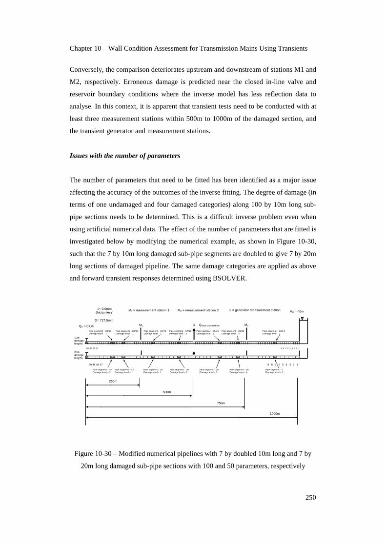
Chapter 10 – Wall Condition Assessment for Transmission Mains Using Transients
250
Conversely, the comparison deteriorates upstream and downstream of stations M1 and
M2, respectively. Erroneous damage is predicted near the closed in-line valve and
reservoir boundary conditions where the inverse model has less reflection data to
analyse. In this context, it is apparent that transient tests need to be conducted with at
least three measurement stations within 500m to 1000m of the damaged section, and
the transient generator and measurement stations.
Issues with the number of parameters
The number of parameters that need to be fitted has been identified as a major issue
affecting the accuracy of the outcomes of the inverse fitting. The degree of damage (in
terms of one undamaged and four damaged categories) along 100 by 10m long sub-
pipe sections needs to be determined. This is a difficult inverse problem even when
using artificial numerical data. The effect of the number of parameters that are fitted is
investigated below by modifying the numerical example, as shown in Figure 10-30,
such that the 7 by 10m long damaged sub-pipe segments are doubled to give 7 by 20m
long sections of damaged pipeline. The same damage categories are applied as above
and forward transient responses determined using BSOLVER.
G QSIDE DISCHARGE
HR = 40m
QV = 0 L/s
ε= 0.0mm (frictionless)
M1 M2
750m
500m
250m
1000m
Pipe segment – 89/90 Damage level – 3
Pipe segment – 13/14 Damage level – 2
Pipe segment – 83/84 Damage level – 1
Pipe segment – 39/40 Damage level – 3
Pipe segment – 69/70 Damage level – 1
Pipe segment – 57/58 Damage level – 2
Pipe segment – 31/32 Damage level – 4
D= 727.5mm
M1 = measurement station 1 M2 = measurement station 2 G = generator measurement station
Pipe segment – 45 Damage level – 3
Pipe segment – 7 Damage level – 2
Pipe segment – 42 Damage level – 1
Pipe segment – 20 Damage level – 3
Pipe segment – 35 Damage level – 1
Pipe segment – 29 Damage level – 2
Pipe segment – 16 Damage level – 4
20mdamage lengths
10mdamage lengths
50 49 48 47 9 8 7 6 5 4 3 2 1
100 99 98 97 9 8 7 6 5 4 3 2 1
Figure 10-30 – Modified numerical pipelines with 7 by doubled 10m long and 7 by
20m long damaged sub-pipe sections with 100 and 50 parameters, respectively

Chapter 10 – Wall Condition Assessment for Transmission Mains Using Transients
251
In addition, a second model is established using a numerical pipeline with 50 by 20m
long sub-pipe sections and damage along 7 by 20m long sub-pipe lengths that
correspond with those defined by the doubled 10m long sub-pipe lengths (also as
shown in Figure 10-30). The same damage categories are again applied and forward
transient responses determined using BSOLVER. The same underlying model
discretisation (10m) is used for both models such that similar predicted responses are
obtained using both models.
Figure 10-31 shows the results of inverse analysis performed using the 100 and 50
parameter models, respectively. The comparison between the artificial and fitted
damage patterns for the 100 parameter model (with 7 by doubled 10m long sub-pipe
sections) is significantly less satisfactory than that obtained for the 50 parameter
model (with 7 by 20m long sub-pipe sections). The fitted pattern of damage obtained
using the 50 parameter model closely matches the artificial pattern. The fitted pattern
of damage obtained using the 100 parameter model includes numerous erroneous
predictions. The 50 parameter model is thought to be more accurate because fewer
parameters are fitted.
650
700
750
800
850
900
950
1000
1050
0 250 500 750 1000
Chainage (m)
Wav
e S
pee
d (
m/s
)
Damage level 1 Damage level 2
Damage level 3 Damage level 4
Wave Speed (m/s) Measurement Points
10m damage lengths 20m damage lengths
M1 M2G
Location at which transient is generated
79%
Approximate % of remaining wall thickness
58%
100%
37%
100%
no CML
Figure 10-31 – Results of inverse analysis using 100 parameter and 50 parameter
models with the same pattern of artificial damage in 20m long sub-pipe lengths

Chapter 10 – Wall Condition Assessment for Transmission Mains Using Transients
252
Figure 10-32 shows the measured artificial response and predicted fitted response at
the transient generator when 10m long and 20m long sub-pipe sections are used to
represent damage, respectively. The results obtained when the model with 50
parameters and 7 by 20m long damaged sub-pipe lengths is used match closely with
the artificial damage pattern. The results obtained when the model with 100
parameters and 7 by doubled 10m long damaged sub-pipe lengths is used match
relatively less closely. This discrepancy is consistent with the more and less accurate
comparison between the artificial and fitted patterns of damage obtained using the 50
and 100 parameter models, respectively.
39.0
40.0
41.0
42.0
43.0
44.0
45.0
46.0
47.0
0.0 0.1 0.2 0.3 0.4 0.5 0.6 0.7 0.8 0.9Time (s)
Pre
ssu
re (
m)
Measured "artificial" response
Predicted "fitted" response - 10m damage lengths
Predicted "fitted" response - 20m damage lengths
Figure 10-32 – Artificial and fitted transient responses at the transient generator
obtained using 100 parameter and 50 parameter numerical models, respectively
Figures 10-33 and 10-34 show the measured artificial responses and predicted fitted
responses at measurement stations M1 and M2, respectively. As at the transient
generator, the results obtained using the 50 parameter model are more accurate than
those obtained using the 100 parameter model. As mentioned above, the 50 parameter
model is thought to be more accurate because fewer parameters are fitted. Further
investigation, beyond the scope of this research is occurring into inverse methods and
algorithms that can be used to fit large numbers of parameters with greater accuracy.

Chapter 10 – Wall Condition Assessment for Transmission Mains Using Transients
253
39.0
40.0
41.0
42.0
43.0
44.0
45.0
46.0
47.0
0.0 0.1 0.2 0.3 0.4 0.5 0.6 0.7 0.8 0.9Time (s)
Pre
ssu
re (
m)
Measured "artificial" response
Predicted "fitted" response - 10m damage lengths
Predicted "fitted" response - 20m damage lengths
39.0
40.0
41.0
42.0
43.0
44.0
45.0
46.0
47.0
0.0 0.1 0.2 0.3 0.4 0.5 0.6 0.7 0.8 0.9Time (s)
Pre
ssu
re (
m)
Measured "artificial" response
Predicted "fitted" response - 10m damage lengths
Predicted "fitted" response - 20m damage lengths
Figure 10-33 and 10-34 – Artificial and fitted transient responses, obtained using 100
and 50 parameter models, at measurement locations 1 and 2, respectively
10.4.7 Application of inverse transient software to pseudo-field pipe
Figure 10-35 shows a representation of the Morgan Transmission Pipeline (MTP)
along the 1.5km section encompassing scour valve 22 and air valves 39 and 41. The
pipeline is 1500m long and 727.5mm in diameter. The pipeline has an estimated
roughness of 3mm and this is included in the transient modelling. Furthermore, the
relative elevation of the pipeline is maintained along its entire length. An assumed
reservoir depth of 32.6m is applied to give similar static pressures to those observed in
the MTP at the locations of scour valve 22 and air valves 39 and 41. As for test 7,
conducted on the MTP in August 2004, the pressure response is determined at three
locations (namely measurement stations 1 and 2 and at the transient generator). These
locations correspond with air valves 39 and 41 and scour valve 22, respectively.
As for the numerical example, and the trial and error fitting described above, four
categories of damage are used to simulate the deterioration of the wall of the MTP
over 10m lengths. The loss of cement mortar lining (CML) without corrosion of the
steel pipeline wall is category 1, and categories 2, 3 and 4 have lost CML and 1mm,
2mm and 3mm of corroded wall thickness, respectively. The different categories of
damage are shown in Figure 10-35 at 45 locations. The first 16 damaged sections
from the closed in-line valve boundary condition are located on the basis of CCTV
camera footage available along this section of the MTP. The next 10 damaged
sections are located on the basis on the results of the trial and error fitting, for test 7
conducted on the MTP, as described above. The last 19 damaged sections up to the
reservoir boundary are located on an arbitrary basis. The category of damage is based

Chapter 10 – Wall Condition Assessment for Transmission Mains Using Transients
254
on the results of the CCTV camera inspection or trial and error fitting over the
relevant sections of the MTP.
G
QSIDE DISCHARGE
HR = 32.6m
QV = 0 L/s M1
M2
Pipe segment – 144Damage level – 1
Pipe segment – 24Damage level – 1
Pipe segment – 139Damage level – 3
Pipe segment – 135/136 Damage level – 1 and 2
Pipe segment – 124Damage level – 2
D= 727.5mm
M1 = measurement station 1 M2 = measurement station 2 G = generator measurement station
Pipe segment – 64/65Damage level – 2 and 1
Pipe segment – 61 Damage level – 2 Pipe segment – 31
Damage level – 3 Pipe segment – 49/50/51Damage level – 2, 3 and 2
Pipe segment – 43Damage level – 1
Pipe segment – 27 Damage level – 2
10m damage lengths
100 99 98 97
9 8 7 6 5 4 3 2 1
Pipe segment – 130/131 Damage level – 3 and 2
Pipe segment – 128Damage level – 1
Pipe segment – 117/118/119/120Damage level – 2, 3, 3, and 2
Pipe segment – 112/113Damage level – 2 and 3 Pipe segment – 110
Damage level – 2
Pipe segment – 105/106/107Damage level – 3, 3, and 3
Pipe segment – 103Damage level – 3
Pipe segment – 98 Damage level – 4
Pipe segment – 95Damage level – 3
Pipe segment – 91 Damage level – 2
Pipe segment – 88 Damage level – 2
Pipe segment – 84 Damage level – 2
Pipe segment – 81 Damage level – 1
Pipe segment – 78 Damage level – 1
Pipe segment – 69 Damage level – 3
Pipe segment – 55 Damage level – 4
Pipe segment – 41 Damage level – 2 Pipe segment – 34/35/36
Damage level – 3, 1 and 3
Pipe segment – 16 Damage level – 3
Pipe segment – 12 Damage level – 2
Pipe segment – 10 Damage level – 3
“Known” pattern of damage from CCTV camera footage Inferred pattern of damage from “trial and error” fitting
“Arbitrary” or “artificial” pattern of damage “Arbitrary” or “artificial” pattern of damage
ε= 3.0mm
Label Chainage Elevation Comment M1 15290m 112.0m Measurement station 1 at air valve 39 G 15710m 114.0m Transient Generator at scour valve 22 M2 15990m 115.5m Measurement station 2 at air valve 41 Closed end valve 14960m 110.0m Artificial closed valve boundary condition Reservoir 16460m 117.5m Artificial reservoir/tank boundary condition
Figure 10-35 – Psuedo-field pipeline used to test the inverse transient model for wall
condition assessment along a representative length of the MTP
Figure 10-36 shows the estimated pattern of damage along the pseudo-field pipeline,
represented in terms of reduction in wave speed and loss of CML and/or corrosion of
wall thickness, and the pattern of damage predicted after performing inverse analysis.
In this problem, 150 sub-pipe segments are used to represent damage along 1500m of
the MTP in 10m lengths. This means that 150 parameters need to be fitted during the
inverse analysis. This is a more difficult inverse problem than tackled numerically
above with an even larger search space. Furthermore, the measurement station
locations are fixed, at the locations of scour valve 22 and air valves 39 and 41, and
cannot be moved to positions that maximise the reflection information used during the
inverse analysis.

Chapter 10 – Wall Condition Assessment for Transmission Mains Using Transients
255
The comparison between the estimated and fitted patterns of damage is not as good as
for the numerical example. Nevertheless, the results are reasonable and the pattern of
damage based on CCTV camera footage, trial and error fitting and a partial arbitrary
distribution is fitted with relative accuracy. Even at this stage, the results provide a
qualified basis upon which to infer the locations at which damage occurs along the
section of the MTP subject to CCTV camera survey (which can be used to check the
pattern of damage derived from the inverse analysis). Errors in the position of
predicted damage along this section are in the order of ±30m while the errors in
magnitude are up to, but generally less than, 50%. As mentioned previously, work is
continuing outside the scope of this research to find methods for improving the
inverse analysis including the identification of better search algorithms.
650
700
750
800
850
900
950
1000
1050
0 250 500 750 1000 1250 1500
Chainage (m)
Wav
e S
pee
d (
m/s
)
Damage level 1 Damage level 2 Damage level 3 Damage level 4
Wave Speed (m/s) Measurement Points Results after fitting
M1 M2G
Location at which transient is generated
79%
Approximate % of remaining wall thickness
58%
100%
37%
100%
no CML
Figure 10-36 – Estimated and predicted patterns of damage along the 1500m long
section of the MTP encompassing scour valve 22 and air valves 39 and 41
Figure 10-37 shows that the measured artificial and predicted fitted responses
determined after the inverse analysis are similar at the location of the transient
generator (i.e., scour valve 22). This is despite the discrepancies between the
estimated and fitted patterns of damage noted above and indicates that the inverse
algorithm is operating on relatively small differences in pressure once the match
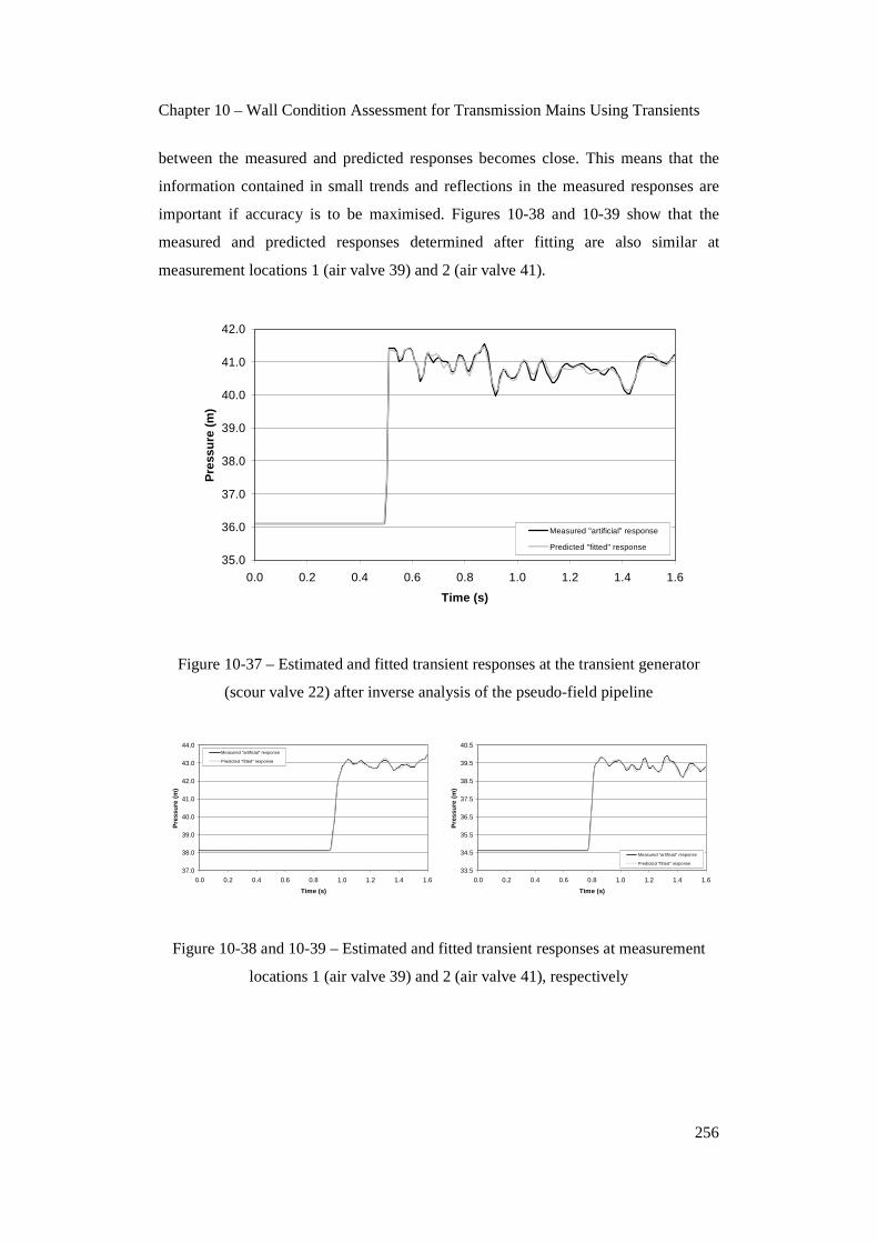
Chapter 10 – Wall Condition Assessment for Transmission Mains Using Transients
256
between the measured and predicted responses becomes close. This means that the
information contained in small trends and reflections in the measured responses are
important if accuracy is to be maximised. Figures 10-38 and 10-39 show that the
measured and predicted responses determined after fitting are also similar at
measurement locations 1 (air valve 39) and 2 (air valve 41).
35.0
36.0
37.0
38.0
39.0
40.0
41.0
42.0
0.0 0.2 0.4 0.6 0.8 1.0 1.2 1.4 1.6
Time (s)
Pre
ssu
re (
m)
Measured "artificial" response
Predicted "fitted" response
Figure 10-37 – Estimated and fitted transient responses at the transient generator
(scour valve 22) after inverse analysis of the pseudo-field pipeline
37.0
38.0
39.0
40.0
41.0
42.0
43.0
44.0
0.0 0.2 0.4 0.6 0.8 1.0 1.2 1.4 1.6
Time (s)
Pre
ssu
re (
m)
Measured "artificial" response
Predicted "fitted" response
33.5
34.5
35.5
36.5
37.5
38.5
39.5
40.5
0.0 0.2 0.4 0.6 0.8 1.0 1.2 1.4 1.6
Time (s)
Pre
ssu
re (
m)
Measured "artificial" response
Predicted "fitted" response
Figure 10-38 and 10-39 – Estimated and fitted transient responses at measurement
locations 1 (air valve 39) and 2 (air valve 41), respectively

Chapter 10 – Wall Condition Assessment for Transmission Mains Using Transients
257
10.5 Summary
The hydraulic noise identified in Chapter 7, and found to be problematic in the
context of Inverse Transient Analysis (ITA) for leak detection in Chapter 9, is
examined in more detail in this chapter. The field tests conducted on the Morgan
Transmission Pipeline (MTP) in August 2004, with a modified nozzle, to reduce the
effects of flow turbulence or “flutter”, exhibited relatively insignificant hydraulic
noise prior to the induction of each controlled transient. However, significant
hydraulic noise was observed following the induction of each transient. This hydraulic
noise was structured and a consistent pattern of reflections was observed for repeated
tests (even with different pipeline boundary conditions). Eventually, the pattern of
reflections was dispersed and damped by a combination of the effects of fluid friction,
entrained air and mechanical motion and vibration (and possibly the formation of
flexural and shear waves).
The condition of the MTP between chainage 15000m and 15400m, 17200m and
17700m and, finally, 16000m and 16400m is described in this chapter based on
CCTV camera investigation and information provided by the South Australian Water
Corporation. This information is used to categorise 10m lengths of the MTP between
the abovementioned chainages in terms of cement mortar lining delamination, wall
corrosion and accumulations of pieces of lining. Physical explanations for the pattern
of structured reflections observed in the measured responses, which may be related to
the condition of the lining and pipe wall, are explored including reflections from
trapped air pockets and discrete protrusions (formed by accumulations of delaminated
lining). These physical mechanisms do not explain the observed reflections. Fluid
Structure Interaction (FSI) has previously been considered in Chapter 7 and does not
account for the observed reflections.
The hypothesis that the structured reflections are related to variations in wave speed
(and pipeline impedance), where lining has delaminated and/or wall corrosion has
occurred, is presented in this chapter. Four different categories of damage to the lining
and wall condition of the MTP, together with the undamaged condition, are described
in terms of wave speed over 10m (and also 5m) lengths of pipeline. Different
distributions of these categories are then applied on a trial and error basis to infer the

Chapter 10 – Wall Condition Assessment for Transmission Mains Using Transients
258
condition of the MTP either side of the section between chainage 15000m and
15400m (for which the condition of the pipeline is known). The objective of the trial
and error process was to match the predicted response, obtained using a forward
transient model, with the measured response using a known or inferred pattern of
damage.
The result has been a reasonable match between the predicted and measured transient
responses using a combination of the known and inferred pipeline condition. This
suggests that the inferred pipeline condition may be representative of the physical
condition of the relevant lengths of pipeline. Significantly, the ability to interpret the
structured reflections using forward transient models, and global optimisation
algorithms (to replace trial and error inference of pipeline condition), may allow
variations in the condition of pipeline linings and walls to be determined using
measured transient responses.

Chapter 11 – Distribution Pipeline Tests and Transient Modelling
259
Chapter 11
Distribution Pipeline Tests and Transient Modelling
_____________________________________________________________________
No reported transient tests or analysis could be identified in the literature for
individual pipelines within water distribution systems. This may be because of the
physical complexity of such pipelines and the difficulties in inducing sufficiently
sharp transients to acquire interpretable reflection information. Details of three
pipelines within water distribution systems, at the scale of individual residential
streets, are introduced in this chapter. The first two pipelines, called the Saint Johns
Terrace Pipeline (SJTP) and Kookaburra Court Pipeline (KCP), are in close
geographical proximity to each other (both being located within a small gravity
distribution system called the Willunga Network). The third pipeline, called the Foster
Street Pipeline (FSP), is geographically remote from the other two and located close
to the City of Adelaide, South Australia. Figure 11-1 shows the location of SJTP and
KCP within the Willunga Network.
The method for generating the transients involved the rapid closure of a side discharge
valve transient generator as described in Chapter 6. Druck PDCR-810 pressure
transducers, mounted inside “dummy” fire plug caps, were typically installed within
existing fire plug chambers. The pressure measurement stations recorded the transient
response of the distribution pipelines at either 500Hz or 2000Hz and were
synchronised, as described in Chapter 6, using voltage pulses transmitted between
stations along cables.
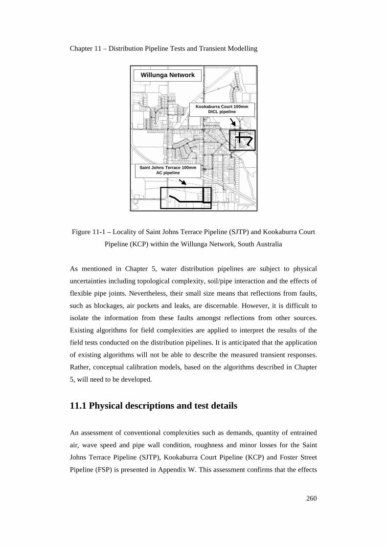
Chapter 11 – Distribution Pipeline Tests and Transient Modelling
260
Willunga Network
Kookaburra Court 100mm DICL pipeline
Saint Johns Terrace 100mm AC pipeline
Figure 11-1 – Locality of Saint Johns Terrace Pipeline (SJTP) and Kookaburra Court
Pipeline (KCP) within the Willunga Network, South Australia
As mentioned in Chapter 5, water distribution pipelines are subject to physical
uncertainties including topological complexity, soil/pipe interaction and the effects of
flexible pipe joints. Nevertheless, their small size means that reflections from faults,
such as blockages, air pockets and leaks, are discernable. However, it is difficult to
isolate the information from these faults amongst reflections from other sources.
Existing algorithms for field complexities are applied to interpret the results of the
field tests conducted on the distribution pipelines. It is anticipated that the application
of existing algorithms will not be able to describe the measured transient responses.
Rather, conceptual calibration models, based on the algorithms described in Chapter
5, will need to be developed.
11.1 Physical descriptions and test details
An assessment of conventional complexities such as demands, quantity of entrained
air, wave speed and pipe wall condition, roughness and minor losses for the Saint
Johns Terrace Pipeline (SJTP), Kookaburra Court Pipeline (KCP) and Foster Street
Pipeline (FSP) is presented in Appendix W. This assessment confirms that the effects

Chapter 11 – Distribution Pipeline Tests and Transient Modelling
261
of demands and entrained air are not significant during the transient tests (because of
precautionary measures taken before the tests). Wave speeds for the three distribution
pipelines are determined on the basis of the timed arrival of wave fronts at different
measurement stations. Pipe roughness is determined using steady state pressure
measurements and significant minor losses are identified.
In the context of below ground (i.e., buried) distribution system pipelines, physical
complexities, in addition to the conventional complexities mentioned above, include
the potential for mechanical motion and vibration as well as effects from complex
water service connection topology, the behaviour of numerous individual flexible
joints and soil/pipe interaction. The response of each of these physical complexities
contributes to dispersion and damping of the measured transient responses of
distribution pipelines. Apart from the theoretical complexities of the response of
flexible joints and soil/pipe interaction, as discussed in Chapter 5, the sheer scope for
physical variation, in terms of the numbers and condition of individual elements,
suggests that the measured transient responses from such pipelines will be highly
complex.
11.1.1 Physical description and test details for the SJTP
Physical description of the Saint Johns Terrace Pipeline (SJTP)
The general details and configuration of the pipeline during testing are shown in
Figure 11-2. The SJTP is 575m long, comprises 100mm nominal diameter “Class D”
Asbestos Cement (AC) pipe (manufactured in accordance with obsolete Australian
Standard AS 1711 – 1975). The SJTP exists as a natural branch on the perimeter of
the Willunga Network and the boundary conditions comprise a “T” intersection with
the main network and a naturally occurring dead end. An existing in-line gate valve
was used to simulate different extents of discrete blockage (as described in Chapter
6). The presence of the in-line gate valve partly along the length of the pipeline was
the main motivation for conducting tests on the SJTP.

Chapter 11 – Distribution Pipeline Tests and Transient Modelling
262
The in-line gate valve is located approximately 382.4m along the pipeline from the
“T” intersection with the main network. An equivalent gate valve, removed from the
Willunga Network, has been calibrated in the laboratories of the University of
Adelaide, at different percentage openings, as described in Appendix I. The transient
generator was installed on a fire plug located 273.5m from the “T” intersection. For a
percentage of the transient tests, a baseflow was established along the SJTP and
through an additional standpipe located at the end of the pipeline. A 25mm diameter
orifice was installed to restrict the magnitude of this baseflow.
Controlled transient source located at central FH with torsional spring generator
Baseflow discharge through 25mm orifice located on standpipe connected to FH
FH – fire hydrant PMS – pressure measurement station
PMS – location 2 FH
FH FH
FH
FH FH
FHFH
15.1m
96.2m 83.4m
78.8m
108.9m
100.8m 91.6m
GATE VALVE – open
Artificial reservoir at tee intersection with network
GATE VALVE – partially closed to simulate discrete blockages
PMS – location 1
PMS – location 3
Typical 25mm water service connections
Figure 11-2 – Basic layout and details of the Saint Johns Terrace Pipeline (SJTP)
The SJTP was manually surveyed, as part of a larger survey of the Willunga Network,
using a “Total Station” electronic level and position survey instrument and this
information was verified using “as constructed” plans as described in Appendix K.
There are 8 fire plugs located at road level along the length of the SJTP. Risers of
various lengths are used to connect these fire plugs to the pipeline. There are 6 by
25mm water service connections.
Each in-line gate valve and fire plug is installed using flexible rubber ring collar joints
as described in Chapter 5. Additional flexible joints are provided at a 3m to 6m
spacing to join the sections of Asbestos Cement (AC) pipe comprising the SJTP. Each

Chapter 11 – Distribution Pipeline Tests and Transient Modelling
263
joint reduces the level of restraint and increases the potential for mechanical losses
(particularly at changes in direction or at dead ends). Soil/pipe interaction is
anticipated because the ratio of the modulus of the backfill in the pipe trenches, as
consolidated by road traffic, to the elastic modulus of the AC pipe (as determined in
the laboratory and specified in Appendix D), is less than 500. Finally, water service
connections are directly connected to the SJTP and water meters are installed on each
water service connection.
Test details for the Saint Johns Terrace Pipeline (SJTP)
On the 23rd July 2003, five controlled transient tests were performed as listed in Table
11-1 which also specifies the configuration of the Saint Johns Terrace Pipeline
(SJTP), including initial flow conditions, whether a side discharge valve closure or
opening was used to induce controlled transients, the size of the nozzle mounted in the
transient generator, recording rate and purpose of each test. The SJTP was in its “in-
situ” condition without baseflow for all five tests.
Table 11-1 – Summary of controlled transient tests for the SJTP on 23rd July 2003
Test Valve Configuration
Flow Condition
Type of Motion
Discharge Nozzle
Recording Stations Rate Purpose
1 Fully open No baseflow Closure 6mm 1, 2 and 3 500Hz “In-situ” condition
2 Fully open No baseflow Closure 8mm 1, 2 and 3 500Hz “In-situ” condition
3 Fully open No baseflow Closure 10mm 1, 2 and 3 500Hz “In-situ” condition
4 Closed No baseflow Closure 6mm 1, 2 and 3 500Hz Closed valve
5 Closed No baseflow Closure 10mm 1, 2 and 3 500Hz Closed valve
On the 15th August 2003, a mix of fourteen controlled transient tests were performed
as listed in Table 11-2, without and with baseflow along the pipeline, and with the in-
line gate valve either open or only partially open. The baseflow was created by
opening a 25mm diameter orifice, mounted on a standpipe, located at the dead end of
the SJTP. Pressure transducers were located at measurement stations 2 and 3 (i.e.,
upstream and downstream of the gate valve) and an 8mm nozzle was installed in the
transient generator.

Chapter 11 – Distribution Pipeline Tests and Transient Modelling
264
Table 11-2 – Summary of controlled transient tests for the SJTP on 15th August 2003
Test Valve Configuration
Flow Condition
Type of Motion
Discharge Nozzle Stations Rate Purpose
1 Fully open No baseflow Closure 8mm 2 and 3 500Hz “In-situ” condition
2 Fully open No baseflow Closure 8mm 2 and 3 500Hz “In-situ” condition
3 Fully open Baseflow Closure 8mm 2 and 3 500Hz “In-situ” condition
4 Fully open Baseflow Closure 8mm 2 and 3 500Hz “In-situ” condition
5 “1/2” turn open Baseflow Closure 8mm 2 and 3 500Hz Discrete blockage
6 “1/2” turn open Baseflow Closure 8mm 2 and 3 500Hz Discrete blockage
7 “1/2” turn open Baseflow Closure 8mm 2 and 3 500Hz Discrete blockage
8 “1/2” turn open Baseflow Closure 8mm 2 and 3 500Hz Discrete blockage
9 “5/8” turn open Baseflow Closure 8mm 2 and 3 500Hz Discrete blockage
10 “5/8” turn open Baseflow Closure 8mm 2 and 3 500Hz Discrete blockage
11 “5/8” turn open Baseflow Closure 8mm 2 and 3 500Hz Discrete blockage
12 “5/8” turn open Baseflow Closure 8mm 2 and 3 500Hz Discrete blockage
13 “1” turn open Baseflow Closure 8mm 2 and 3 500Hz Discrete blockage
14 “1” turn open Baseflow Closure 8mm 2 and 3 500Hz Discrete blockage
On the 26th August 2003, a mix of ten controlled transient tests were performed as
listed in Table 11-3, with baseflow along the pipeline, and with the in-line gate valve
either open or only partially open. Pressure transducers were located at measurement
stations 1 and 2 (i.e., both upstream of the gate valve) and an 8mm nozzle was
installed in the transient generator.
Table 11-3 – Summary of controlled transient tests for the SJTP on 26th August 2003
Test Valve Configuration
Flow Condition
Type of Motion
Discharge Nozzle Stations Rate Purpose
1 Fully open Baseflow Closure 8mm 1 and 2 500Hz In-situ condition
2 Fully open Baseflow Closure 8mm 1 and 2 500Hz In-situ condition
3 “1/2” turn open Baseflow Closure 8mm 1 and 2 500Hz Discrete blockage
4 “1/2” turn open Baseflow Closure 8mm 1 and 2 500Hz Discrete blockage
5 “1/2” turn open Baseflow Closure 8mm 1 and 2 500Hz Discrete blockage
6 “1/2” turn open Baseflow Closure 8mm 1 and 2 500Hz Discrete blockage
7 “1/2” turn open Baseflow Closure 8mm 1 and 2 2000Hz Discrete blockage
8 “1/2” turn open Baseflow Closure 8mm 1 and 2 2000Hz Discrete blockage
9 “1/2” turn open Baseflow Closure 8mm 1 and 2 2000Hz Discrete blockage
10 “1/2” turn open Baseflow Closure 8mm 1 and 2 2000Hz Discrete blockage

Chapter 11 – Distribution Pipeline Tests and Transient Modelling
265
The transients induced in the SJTP on the 23rd July 2003 gave maximum pressure
rises of approximately 90kPa and 130kPa for the 8mm and 10 mm discharge nozzles,
respectively. Similar transient pressure rises were induced during the tests conducted
on the 15th and 26th August 2003. These pressure rises did not concern operators from
United Water. Data was recorded over a limited period of 0.8s. This time marginally
exceeded that required for the transient wavefront to travel to the open “T”
intersection and return to the nearest measurement station location.
11.1.2 Physical description and test details for the KCP
Physical description of the Kookaburra Court Pipeline (KCP)
The general details and configuration of the pipeline during testing are shown in
Figure 11-3 together with the locations at which an artificial air pocket and leak were
introduced along the KCP. The details of the artificial air pocket and leak were
described in Chapter 6. The transient generator was installed on a fire plug located
318.1m from the “T” intersection. The method for generating the transients involved
both the rapid closure and opening of a side discharge valve.
The KCP is 379.2m long, comprises 100mm nominal diameter “Class K9” Ductile
Iron Cement Mortar Line (DICL) pipe (manufactured in accordance with Australian
Standard AS 2280 – 1999) and forms part of the Willunga Network. The KCP exists
as a natural branch on the perimeter of the Willunga Network and the boundary
conditions comprise a “T” intersection with the main network and a naturally
occurring dead end. An artificial air pocket and leak were introduced as known faults.
The location of the KCP at the extremity of the Willunga Network, and the fact that it
was DICL, were the main motivations for conducting tests on the KCP.

Chapter 11 – Distribution Pipeline Tests and Transient Modelling
266
Controlled transient source located at FH with torsional spring generator
FH – fire hydrant PMS – pressure measurement station
FH
FH
FH
FH
FH
73.0m
81.3m
70.7m 93.1m
40.1m
20.0m
GATE VALVE – open
PMS – location 1
PMS – location 2 Artificial air chamber
Artificial 10mm leak
Typical 25mm water service connections
Artificial reservoir at tee intersection with network
Figure 11-3 – Basic layout and details of the Kookaburra Court Pipeline (KCP)
The KCP was manually surveyed, as part of a larger survey of the Willunga Network,
using a “Total Station” electronic level and position survey instrument and this
information was verified using “as constructed” plans as described in Appendix K.
There are 5 fire plugs located at road level along the length of the KCP. Risers of
various lengths are used to connect these fire plugs to the pipeline. A 90 degree bend
is located approximately 20m from the dead end of the KCP. There are 15 by 25mm
water service connections.
Each in-line gate valve and fire plug is installed using flexible spigot and socket joints
as described in Chapter 5. Additional flexible joints are provided at a 3m to 6m
spacing to join the sections of Ductile Iron Cement Lined (DICL) pipe comprising the
KCP. The effect of soil/pipe interaction is expected to be less significant for the KCP
because the ratio of the modulus of the backfill in the pipe trenches, as consolidated
by road traffic, to the elastic modulus of the DICL pipe is greater than 500. That said,
the larger number of water service connections add significantly to the physical
complexity of the pipeline.

Chapter 11 – Distribution Pipeline Tests and Transient Modelling
267
Test details for the Kookaburra Court Pipeline (KCP)
On the 28th August 2003, twelve controlled transient tests were performed as listed in
Table 11-4 which also specifies the configuration of the Kookaburra Court Pipeline
(KCP), including initial flow conditions, whether a side discharge valve closure or
opening was used to induce controlled transients, the size of the nozzle mounted in the
transient generator, recording rate and purpose of each test. The KCP was either in its
“in-situ” condition or had an artificial air pocket or leak installed at the locations
shown above, and using the fittings, described in Chapter 6.
Table 11-4 – Summary of controlled transient tests for the KCP on 28th August 2003
Test Configuration Type of Motion
Discharge Nozzle
Recording Stations Rate Purpose
1 No air pocket or leak Closure 6mm 1 and 2 500Hz “In-situ” condition
2 No air pocket or leak Closure 6mm 1 and 2 500Hz “In-situ” condition
3 No air pocket or leak Opening 6mm 1 and 2 500Hz “In-situ” condition
4 No air pocket or leak Opening 6mm 1 and 2 500Hz “In-situ” condition
5 No air pocket or leak Opening 6mm 2 2000Hz “In-situ” condition
6 No air pocket or leak Opening 6mm 2 2000Hz “In-situ” condition
7 No air pocket or leak Closure 6mm 2 2000Hz “In-situ” condition
8 1.635L air pocket Opening 6mm 1 and 2 500Hz Air pocket response
9 1.635L air pocket Opening 6mm 1 and 2 500Hz Air pocket response
10 10 mm leak Opening 6mm 2 500Hz Leak response
11 10 mm leak Opening 6mm 2 500Hz Leak response
12 10 mm leak Opening 6mm 2 2000Hz Leak response
As reported in Table 11-4, side discharge valve closures and openings were used to
generate controlled transients in the KCP on the 28th August 2003. Positive transients
(i.e., transients associated with an increase in pressure in the pipeline) were induced in
the KCP by closing the side discharge valve giving an initial maximum pressure rise
of approximately 65kPa at station 2. A maximum pressure rise of 105kPa was
recorded after wavefront reflection from the dead end of the KCP.
Negative transients (i.e., transients associated with a decrease in pressure in the
pipeline) were induced in the KCP by opening the side discharge valve giving an

Chapter 11 – Distribution Pipeline Tests and Transient Modelling
268
initial minimum pressure drop of approximately 55kPa at station 2. A minimum
pressure drop of 105kPa was recorded after wavefront reflection from the dead end of
the KCP. Data was recorded over a limited period of 0.7s. This time marginally
exceeded that required for the transient wavefront to travel to the open “T”
intersection and return to the nearest measurement station.
11.1.3 Physical description and test details for the FSP
Physical description of the Foster Street Pipeline (FSP)
The general details and configuration of the pipeline during testing are shown in
Figure 11-4. The FSP is approximately 358.2m long by 80mm nominal diameter Cast
Iron Cement Mortar Line (CICL) pipe. The pipeline was not manufactured in
accordance with any known standard and was laid in 1932. The FSP exists as a
connecting pipeline within a grid-like larger network and the boundary conditions
comprise “T” intersections at either end. The main motivation for conducting tests on
the FSP was a record of low pressure and water quality complaints from two residents
near the middle of the street. It was thought that these complaints indicated the
presence of tuberculation along the parts of the pipeline.
Controlled transient source located at FH with torsional spring generator – locations 1 and 2
FH – fire hydrant PMS – pressure measurement station
FH
FH
81.1m 72.0m
75.6m
18.0m
84.6m
GATE VALVE – open Typical 20mm water service connections
Artificial reservoir at tee intersection with network
FH FHFH
29.0m
18.0m
GATE VALVE – closed
2 1
PMS – location 2
PMS – location 1
Figure 11-4 – Basic layout and details of the Foster Street Pipeline (FSP)

Chapter 11 – Distribution Pipeline Tests and Transient Modelling
269
“Total Station” survey was not undertaken for the FSP because United Water
operators had obtained manual survey information in order to develop a contract for
the replacement of the pipeline in April 2005. This survey information was compared
to existing “as constructed” records and the plan and elevation information describing
the FSP was found to be consistent. There are 5 fire plugs located at road level along
the length of the FSP. Risers of various lengths are used to connect these fire plugs to
the pipeline. There are 22 by 20mm water service connections.
Each in-line gate valve and fire plug is installed using flexible spigot and socket joints
as described in Chapter 5. Additional flexible joints are provided at a 3m to 6m
spacing to join the sections of Cast Iron Cement Lined (CICL) pipe comprising the
FSP. As for the Kookaburra Court Pipeline (KCP), the effect of soil/pipe interaction is
expected to be less significant than for the Saint Johns Terrace Pipeline (SJTP).
However, there is a greater number of water service connections for the FSP than
KCP as well as existing sections of pipeline with significant tuberculation.
Given that the FSP was not a natural branch, it was necessary to close the in-line gate
valve at the western end of the pipeline to isolate it from the influence of the existing
network beyond this location. At the same time, the in-line gate valve at the eastern
end of the pipeline needed to remain open to maintain continuity of supply to the
residents and transient generator. In effect, the local network was decomposed to
favourably configure the FSP for the transient tests without interrupting supply. The
formation of an artificial branch pipeline allowed the FSP to be individually assessed.
The concept of network decomposition is further explained in Appendix W. Transient
inputs were generated at two locations to increase the likelihood of identifying
reflections from either end of any tuberculated sections.
Test details for the Foster Street Pipeline (FSP)
On the 16th July and 7th August 2003, four controlled transient tests were performed as
listed in Table 11-5 which also specifies whether a side discharge valve closure or
opening was used, the size of the nozzle mounted in the transient generator and

Chapter 11 – Distribution Pipeline Tests and Transient Modelling
270
recording rate. The purpose of the tests was to obtain measured transient responses
from a pipeline with in-situ extended blockage (i.e., tuberculation).
Table 11-5 – Summary of controlled transient tests for the FSP on the 16th July and 7th
August 2003
Test Date Transient Generator Location
Type of Motion
Discharge Nozzle
Recording Stations Rate
1 16/07/2003 Station 1 Closure 6mm 1 and 2 500Hz
2 16/07/2003 Station 1 Closure 6mm 1 and 2 500Hz
3 7/08/2003 Station 2 Closure 6mm 1 and 2 500Hz
4 7/08/2003 Station 2 Closure 6mm 1 and 2 500Hz
11.2 Positive and negative transients for the KCP
Figure 11-5 shows the response of the Kookaburra Court Pipeline (KCP), measured at
station 2, to controlled positive transients. Various features are apparent in the
measured response including reflections from the dead end of the KCP and the “T”
intersection with the Willunga Network at approximately 0.21s and 0.55s,
respectively. A collapse and then partial recovery in the pressure plateau following the
reflection from the dead end is apparent. Distinct reflections in the response of the
KCP, which cannot be attributed to any known element, are apparent. These
reflections represent the cumulative response of the combined physical complexities
of the KCP. The oscillation following the induction of the transient is due to “ringing”
in the transient generator and will be discussed later in this chapter.
Figure 11-6 shows the response of the KCP, measured at station 2, to controlled
negative transients. Various features are again apparent in the measured response
including reflections from the dead end of the KCP and the “T” intersection with the
Willunga Network at approximately 0.21s and 0.55s, respectively. Notably, there is
no collapse in the magnitude of the negative pressure plateau after the reflection from
the dead end of the KCP. As for positive transient test, distinct reflections in the
response of the KCP, which cannot be attributed to any known element, are apparent.
However, there appears to be significantly less damping.

Chapter 11 – Distribution Pipeline Tests and Transient Modelling
271
42
44
46
48
50
0 0.1 0.2 0.3 0.4 0.5 0.6 0.7
Time (s)
Pre
ssu
re (
m)
Test 1 - Station 2
Test 2 - Station 2
Doubled reflection from dead end
Initial wavefront
Reflection from "T" intersection
26
28
30
32
34
0 0.1 0.2 0.3 0.4 0.5 0.6 0.7
Time (s)
Pre
ssu
re (
m)
Test 3 - Station 2
Test 4 - Station 2
Doubled reflection from dead end
Reflection from "T" intersection
Figures 11-5 and 11-6 – Measured responses for tests 1 and 2 and tests 3 and 4,
conducted on 28th August 2003, over 0.7 seconds at station 2
The induction of positive and negative transients in the KCP, and the responses to
each, provides an important insight into the effect of the physical complexities,
including mechanical motion and vibration, flexible joints and soil/pipe interaction,
and how they might be acting to disperse and damp the observed transients. Figure
11-7 shows the dimensionless comparison of measured responses for test 1, a positive
transient, and test 3, a negative transient (inverted), at station 2. The initial
dimensionless pressure rise for both tests is approximately 1.
-0.5
0.0
0.5
1.0
1.5
2.0
2.5
0 0.1 0.2 0.3 0.4 0.5 0.6 0.7Time (s)
(H-H
S)/
HJo
uko
wsk
y
Test 1 - Station 2 Test 3 - Station 2
Greater pressure loss after reflection from dead end for "positive" vs "negative" transient
Figure 11-7 – Measured positive response for test 1 versus inverted negative response
for test 3 over 0.7 seconds at station 2

Chapter 11 – Distribution Pipeline Tests and Transient Modelling
272
A significant discrepancy emerges between the responses to the positive and negative
transients after the reflection from the dead end of the KCP. A collapse in the pressure
plateau is evident for test 1. In contrast, the pressure plateau is relatively constant for
the negative transient induced during test 3 (as inverted). The fact that no positive
thrust is exerted at the dead end of the KCP may partly explain these observations.
Instead of a volume of water being forced into and along the KCP towards the dead
end, following the induction of a positive transient, a volume of water is abstracted
from the KCP, including the section up to the dead end, and this creates a negative
thrust or pulls on the dead end. Furthermore, physical complexities such as water
service connections, fire plugs and risers, existing roughness and flexible joints may
dissipate more energy following a rapid increase in pressure (i.e., for a positive
transient) as axial and outward circumferential thrust is transferred, via mechanical
vibration and/or movement, to surrounding soils.
The proposed hypothesis is therefore that there is considerable mechanical motion and
vibration at flexible joints (sliding friction) due to variable restraint from soil/pipe
(joint) interaction and that this is responsible for a significant proportion of the
observed dispersion and damping of the measured responses of the KCP (and also
other distribution pipelines with similar physical complexity). The observation that
more damping occurs when the pressure is increased, as opposed to when it is
decreased, supports the hypothesis. There are numerous precedents in other fields of
engineering where mechanical friction and damping (directly proportional to a
pressure increase or internal dynamic load in the case of a positive transient) is
replicated using equivalent “viscous” dispersion and damping. This hypothesis forms
part of the justification for the development of the conceptual transient model
proposed in Chapter 5.
11.3 Development of traditional transient models
As mentioned in Chapter 7, an explicit Method of Characteristics (MOC) scheme has
been implemented in a transient model (called BSOLVER) to determine the response
of single and branched pipe systems. The model includes algorithms for the
calculation of the effect of unsteady friction and discrete air pockets and/or entrained

Chapter 11 – Distribution Pipeline Tests and Transient Modelling
273
air, as elaborated in Appendices E and O, and a listing of the Fortran source code
developed by the author is included in Appendix M.
The program is applied to conduct the forward transient modelling of the Saint Johns
Terrace Pipeline (SJTP) and the Kookaburra Court Pipeline (KCP) reported below.
The forward transient modelling of the Foster Street Pipeline (FSP) is conducted
using the same program in Chapter 13 after the detailed condition of the pipeline,
including the extent of tuberculation, is described. The forward transient program is
modified and linked to the NLFIT suite of Bayesian non-linear regression programs,
developed by Kuczera (1994), in order to perform the inverse analysis described in
Chapters 12, 13 and 14. The modified subroutines developed by the author for this
analysis are presented in Appendix M.
The results of the forward transient modelling will be compared to the measured
responses from the SJTP and KCP without any artificially introduced faults in this
chapter. Complex calibrated conceptual models will be investigated in Chapter 12.
Comparisons between measured and predicted transient responses obtained using
traditional and more complex calibrated conceptual models, with artificial faults, are
presented in Chapters 13 and 14.
11.3.1 Traditional model for the Saint Johns Terrace Pipeline
The Saint Johns Terrace Pipeline (SJTP) has a total length of 574.8m and is
discretised into 496 sub-pipe segments (each 1.16m long). A wave speed varying
between 1061m/s and 1159m/s is applied giving a time step in the calculations of 1ms
and a minimum Courant number of 0.915. A linear timeline interpolation scheme is
implemented in the model and a pipe roughness of 1mm is used. The wave speeds and
pipe roughness are taken from the assessment presented in Appendix W. The transient
generator is located approximately 273.5m along the pipeline measured from the open
“T” intersection end. Boundary conditions are formed by the natural dead end of the
SJTP and the open “T” intersection with the network. The pressure at the “T”
intersection is varied to match the measured pressure at the start of each transient test

Chapter 11 – Distribution Pipeline Tests and Transient Modelling
274
but is not thereafter adjusted (i.e., the pressure at the “T” intersection is not a variable
boundary condition).
It was not possible to accurately survey the 6 private water service connections along
the SJTP. Even if the original details of the pipe work had been able to be ascertained,
the physical condition of the plumbing, at the time of the tests, was unknown. As a
consequence, the 6 water service connections have been approximated by including
10m long branches of 25mm diameter pipe at each offtake. Individual water meters
are represented using 20mm orifices located approximately 3.5m along each offtake
(measured from the SJTP). The transient generator, and other vertical risers beneath
the fire plugs along the SJTP, have been included in the forward transient model as
vertical branches using the nearest multiple of the sub-pipe segment length.
Results of traditional transient modelling without baseflow
Figures 11-8 and 11-9 show the comparison between the measured and predicted
responses, obtained using a traditional forward transient model with unsteady friction
over a time scale of 0.8s, at station 1, for tests 2 and 3 from the 23rd July 2003,
respectively. Discrepancies, comprising a loss and then recovery of pressure along the
measured transient plateau, relative to the predicted response, are apparent following
the arrival of the incident wavefront. Further discrepancies, following the arrival of
the reflection from the “T” intersection are not relevant to the analysis because an
artificial boundary condition is assumed at the “T” intersection.
26
30
34
38
42
46
0 0.1 0.2 0.3 0.4 0.5 0.6 0.7 0.8
Time (s)
Pre
ssu
re (
m)
Measured response Predicted response
Maximum "plateau" discrepancy
Reflections from double fire plugsReflection from "T" intersection vs aritificial tank
26
30
34
38
42
46
0 0.1 0.2 0.3 0.4 0.5 0.6 0.7 0.8
Time (s)
Pre
ssu
re (
m)
Measured response Predicted response
Reflection from "T" intersection vs aritificial tank
Maximum "plateau" discrepancy
Reflections from double fire plugs
Figures 11-8 and 11-9 – Measured and predicted responses for tests 2 and 3, with
8mm and 10mm nozzles and without baseflow, at station 1

Chapter 11 – Distribution Pipeline Tests and Transient Modelling
275
Figures 11-10 and 11-11 show the comparison between the measured and predicted
responses, obtained using a traditional forward transient model with unsteady friction
over a time scale of 0.8s, at station 2, for tests 2 and 3 from the 23rd July 2003,
respectively. Discrepancies, comprising a loss and then recovery of pressure along the
measured transient plateau, relative to the predicted response, are again apparent. The
forward transient model approximately reproduces a “ringing” effect at the transient
generator, associated with the standpipe between the nozzle and the SJTP below, and
the reflections from known point features including the fire plug risers either side of
the in-line gate valve.
33
37
41
45
49
53
0 0.1 0.2 0.3 0.4 0.5 0.6 0.7 0.8
Time (s)
Pre
ssu
re (
m)
Measured response Predicted response
Maximum "plateau" discrepancy
Reflections from double fire plugs
Reflection from "T" intersection vs aritificial tank
33
37
41
45
49
53
0 0.1 0.2 0.3 0.4 0.5 0.6 0.7 0.8
Time (s)
Pre
ssu
re (
m)
Measured response Predicted response
Reflection from "T" intersection vs aritificial tank
Reflections from double fire plugs
Maximum "plateau" discrepancy
Figures 11-10 and 11-11 – Measured and predicted responses for tests 2 and 3, with
8mm and 10mm nozzles and without baseflow, at station 2
Results of traditional transient modelling with baseflow
Figures 11-12 and 11-13 show the comparison between the measured and predicted
responses, obtained using a traditional forward transient model with unsteady friction
over a time scale of 0.8s, for test 3 from the 15th August 2003, conducted with
baseflow, at stations 2 and 3, respectively. The comparison at station 2 shows that
there is a discrepancy along the transient plateau that is similar to that observed
without baseflow. The comparison at station 3 shows a discrepancy along the transient
plateau and between the measured and predicted reflection from the discharging
orifice used to establish the baseflow at the dead end of the Saint Johns Terrace
Pipeline (SJTP).

Chapter 11 – Distribution Pipeline Tests and Transient Modelling
276
11
13
15
17
19
21
23
0 0.1 0.2 0.3 0.4 0.5 0.6 0.7 0.8
Time (s)
Pre
ssu
re (
m)
Measured response Predicted response
Initial underestimation of pressure rise
Reflection from "T" intersection vs aritificial tank
22
24
26
28
30
32
34
0 0.1 0.2 0.3 0.4 0.5 0.6 0.7 0.8
Time (s)
Pre
ssu
re (
m)
Measured response Predicted response
Discrepancy along "plateau" and pressure relief at discharging 25mm orifice at dead end
Figures 11-12 and 11-13 – Measured and predicted responses for test 3, with an 8mm
nozzle and with baseflow, at stations 2 and 3
Figures 11-14 and 11-15 show the comparison between the measured and predicted
responses, obtained using a traditional forward transient model with unsteady friction
over a time scale of 0.8s, for test 1 from the 26th August 2003, conducted with
baseflow, at stations 1 and 2, respectively. The comparison at both stations again
reveals a discrepancy between the measured and predicted responses along the
transient plateaus.
5
7
9
11
13
15
17
0 0.1 0.2 0.3 0.4 0.5 0.6 0.7 0.8
Time (s)
Pre
ssu
re (
m)
Measured response Predicted response
Reflection from "T" intersection vs aritificial tank
Initial underestimation of pressure rise
11
13
15
17
19
21
23
0 0.1 0.2 0.3 0.4 0.5 0.6 0.7 0.8
Time (s)
Pre
ssu
re (
m)
Measured response Predicted response
Reflection from "T" intersection vs aritificial tank
Initial underestimation of pressure rise
Figures 11-14 and 11-15 – Measured and predicted responses for test 1, with an 8mm
nozzle and with baseflow, at stations 1 and 2
Transient generator effect for the Saint Johns Terrace Pipeline
The 1.25m high transient generator standpipe, in combination with the rapid closure
of the 15mm diameter ball valve regulating discharge through the nozzles, over
approximately 4ms, produces a short lived and localised oscillating pressure response
within the standpipe described above and hereafter as “ringing” (a more stable rise or

Chapter 11 – Distribution Pipeline Tests and Transient Modelling
277
fall in pressure is established in the main pipeline). Figure 11-16 shows the measured
transient responses at station 2, recorded at rates of 500Hz and 2000 Hz, for tests 5
and 7, conducted on the 15th and 26th August 2003, respectively. Discrepancies are
apparent between the responses measured at 500Hz and 2000Hz with the form of the
“ringing” better captured at the higher frequency. The higher frequency oscillations
damp out within approximately 0.05s following the induction of the transient.
22
27
32
37
42
47
52
0.09 0.1 0.11 0.12 0.13 0.14
Time (s)
Pre
ssu
re (
m)
Test 5 - 15th Aug Station 2 at 500Hz
Test 7 - 26th Aug Station 2 at 2000Hz
Figure 11-16 – Measured responses for tests 5 and 7, at station 2, over 0.05 seconds,
recorded at 500Hz and 2000Hz, respectively
At the time the tests were conducted, no other practical way of mounting a side
discharge standpipe, with a rapid operation valve mechanism, on fire plug valves
located in underground access chambers had been developed. Furthermore, access to
the main pipe can generally only be achieved through existing fire plugs.
Significantly, these fire plugs are mounted on 0.5m to 1.5m long vertical risers, as the
embedment depth of the main varies, so that a standard access chamber depth of 0.9m
can be maintained. As a consequence, transients induced through existing fire plugs
will exhibit some form of oscillatory response, regardless of whether a transient
generator standpipe or some other device is used. That said, the magnitude of the
oscillatory effect can be reduced if the combined length of standpipe and riser is
minimised.
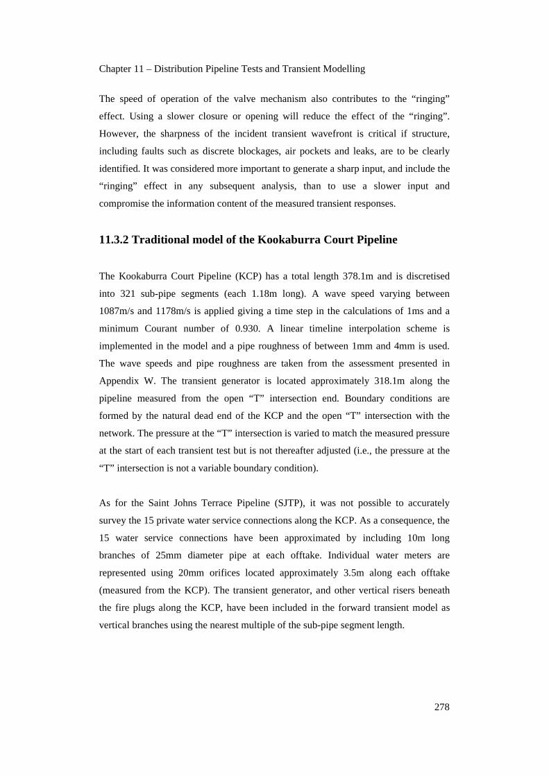
Chapter 11 – Distribution Pipeline Tests and Transient Modelling
278
The speed of operation of the valve mechanism also contributes to the “ringing”
effect. Using a slower closure or opening will reduce the effect of the “ringing”.
However, the sharpness of the incident transient wavefront is critical if structure,
including faults such as discrete blockages, air pockets and leaks, are to be clearly
identified. It was considered more important to generate a sharp input, and include the
“ringing” effect in any subsequent analysis, than to use a slower input and
compromise the information content of the measured transient responses.
11.3.2 Traditional model of the Kookaburra Court Pipeline
The Kookaburra Court Pipeline (KCP) has a total length 378.1m and is discretised
into 321 sub-pipe segments (each 1.18m long). A wave speed varying between
1087m/s and 1178m/s is applied giving a time step in the calculations of 1ms and a
minimum Courant number of 0.930. A linear timeline interpolation scheme is
implemented in the model and a pipe roughness of between 1mm and 4mm is used.
The wave speeds and pipe roughness are taken from the assessment presented in
Appendix W. The transient generator is located approximately 318.1m along the
pipeline measured from the open “T” intersection end. Boundary conditions are
formed by the natural dead end of the KCP and the open “T” intersection with the
network. The pressure at the “T” intersection is varied to match the measured pressure
at the start of each transient test but is not thereafter adjusted (i.e., the pressure at the
“T” intersection is not a variable boundary condition).
As for the Saint Johns Terrace Pipeline (SJTP), it was not possible to accurately
survey the 15 private water service connections along the KCP. As a consequence, the
15 water service connections have been approximated by including 10m long
branches of 25mm diameter pipe at each offtake. Individual water meters are
represented using 20mm orifices located approximately 3.5m along each offtake
(measured from the KCP). The transient generator, and other vertical risers beneath
the fire plugs along the KCP, have been included in the forward transient model as
vertical branches using the nearest multiple of the sub-pipe segment length.
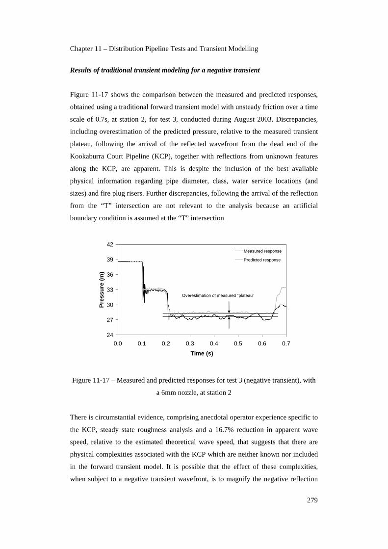
Chapter 11 – Distribution Pipeline Tests and Transient Modelling
279
Results of traditional transient modeling for a negative transient
Figure 11-17 shows the comparison between the measured and predicted responses,
obtained using a traditional forward transient model with unsteady friction over a time
scale of 0.7s, at station 2, for test 3, conducted during August 2003. Discrepancies,
including overestimation of the predicted pressure, relative to the measured transient
plateau, following the arrival of the reflected wavefront from the dead end of the
Kookaburra Court Pipeline (KCP), together with reflections from unknown features
along the KCP, are apparent. This is despite the inclusion of the best available
physical information regarding pipe diameter, class, water service locations (and
sizes) and fire plug risers. Further discrepancies, following the arrival of the reflection
from the “T” intersection are not relevant to the analysis because an artificial
boundary condition is assumed at the “T” intersection
24
27
30
33
36
39
42
0.0 0.1 0.2 0.3 0.4 0.5 0.6 0.7
Time (s)
Pre
ssu
re (
m)
Measured response
Predicted response
Overestimation of measured "plateau"
Figure 11-17 – Measured and predicted responses for test 3 (negative transient), with
a 6mm nozzle, at station 2
There is circumstantial evidence, comprising anecdotal operator experience specific to
the KCP, steady state roughness analysis and a 16.7% reduction in apparent wave
speed, relative to the estimated theoretical wave speed, that suggests that there are
physical complexities associated with the KCP which are neither known nor included
in the forward transient model. It is possible that the effect of these complexities,
when subject to a negative transient wavefront, is to magnify the negative reflection

Chapter 11 – Distribution Pipeline Tests and Transient Modelling
280
from the dead end of the KCP. In this context, the behaviour of the dead end of the
KCP, when subject to suction or pulling thrust during a negative transient, is a major
uncertainty. The results from the negative transient tests (e.g., test 3) are used to
develop a conceptual calibration model in Chapter 12 because the measured responses
appear less affected by mechanical friction and damping (relative to the measured
responses for the positive transients).
Transient generator effect for the Kookaburra Court Pipeline
As for the results from the tests on the Saint Johns Terrace Pipeline (SJTP), the 1.25m
high transient generator standpipe, in combination with the rapid closure or opening
of the 15mm diameter ball valve regulating discharge through the nozzles, over
approximately 4ms, produces a short lived and localised oscillating pressure response
within the standpipe (“ringing”). Figure 11-18 shows the measured transient responses
at station 2, recorded at rates of 500Hz and 2000 Hz, for tests 1 and 7, conducted on
the 28th August 2003, respectively. Discrepancies are apparent between the responses
measured at 500Hz and 2000Hz with the form of the “ringing” effect for these
positive transient tests better captured at the higher frequency. The high frequency
oscillations damp out within approximately 0.03s following the induction of the
positive transients.
Figure 11-19 shows the measured transient responses at station 2, recorded at rates of
500Hz and 2000Hz, for tests 3 and 5, conducted on the 28th August 2003,
respectively. The “ringing” effect for these negative transient tests is better captured at
a recording rate of 2000Hz over the first 0.05s of the responses. The high frequency
oscillations damp out within approximately 0.02s. The magnitude of oscillation
induced following the negative transients is significantly reduced relative to that
following the positive transients. It is likely that sustained discharge through the 6mm
nozzle is responsible for the extra damping.

Chapter 11 – Distribution Pipeline Tests and Transient Modelling
281
35
39
43
47
51
55
0.09 0.10 0.11 0.12 0.13
Time (s)
Pre
ssu
re (
m)
Test 1 - Station 2 at 500Hz
Test 7 - Station 2 at 2000Hz
30
32
34
36
38
40
0.09 0.10 0.11 0.12 0.13
Time (s)
Pre
ssu
re (
m)
Test 3 - Station 2 at 500Hz
Test 5 - Station 2 at 2000Hz
Figures 11-18 and 11-19 – Measured responses for tests 1 and 7, and tests 3 and 5, at
station 2, over 0.04 seconds, recorded at 500 and 2000Hz, respectively
11.4 Summary
Physical complexities relevant to distribution pipelines have been summarised in this
chapter and include pipe, valve, flexible joint and water service connection elements.
When subject to a transient event, these physical components can provide conditions
suitable for, or contribute to, effects from mechanical motion and vibration
(particularly at flexible joints) and soil/pipe interaction. Controlled transient tests
performed on three distribution pipelines, the Saint Johns Terrace Pipeline (SJTP), the
Kookaburra Court Pipeline (KCP) and the Foster Street Pipeline (FSP), are listed in
this chapter. Results are presented for the SJTP and the KCP. The results of the tests
on the FSP are presented in Chapter 13.
Traditional transient models have been developed in this chapter to obtain predicted
transient responses for comparison with the measured responses. Comparisons
between the measured and predicted response of the SJTP have been presented for the
tests conducted with the pipeline in its in-situ condition. Some tests were conducted
with a baseflow to determine the in-situ response of the SJTP, without discrete
blockage, under these conditions. The significance of conducting tests with a baseflow
is explained, in the context of blockage detection, in Chapter 13. Significant
discrepancies between the measured and predicted responses have been identified in
this chapter (for tests without and with baseflow). Explanations for these
discrepancies, and the development of a conceptual calibration model for the SJTP to
account for them, are investigated in Chapter 12.

Chapter 11 – Distribution Pipeline Tests and Transient Modelling
282
A comparison between the measured and predicted response of the KCP, for a test
conducted by opening the side discharge valve in the transient generator, and inducing
a negative transient, has been presented for the pipeline in its in-situ condition. As for
the SJTP, discrepancies between the measured and predicted responses have been
identified. The development of a conceptual calibration model for the KCP is
presented in Chapter 12.
The effect of the standpipe, as part of the transient generator, has been presented in
this chapter. A significant oscillation is introduced to the measured responses obtained
at the location of the transient generator regardless of whether a side discharge closure
or opening is performed. This oscillation has been labelled “ringing” and reduces the
interpretable reflection information near the location of the transient generator.
Modifications to the transient generator are currently being performed, outside of the
scope of this research, to reduce the “ringing” effect.

Chapter 12 – Development of Transient Models for Distribution Pipelines
283
Chapter 12
Development of Transient Models for Distribution
Pipelines
_____________________________________________________________________
Based on the calibration model presented in Chapter 5, and the development and
calibration of such a model for the Hanson Transmission Pipeline (HTP), as presented
in Chapter 8, conceptual calibration models are developed and calibrated, for both the
SJTP and KCP, in this chapter. As for the model developed in Chapter 8, Kelvin-
Voigt mechanical elements are used to introduce a “viscous” mechanism to
approximate equivalent mechanical dispersion and damping. However, the models
developed in this chapter utilise multiple Kelvin-Voigt mechanical elements, with
different creep deformation spring and retardation time dashpot parameters,
distributed spatially in distinct zones along each pipeline to replicate increased
physical variability. This significantly increases the number of parameters used to
calibrate the proposed models and regression diagnostics are examined to identify
signs of redundancy in model structure or parameter correlations indicative of an
over-parameterised model. The sensitivity of the calibration to the number of spatial
zones for each pipeline, and hence also the number of Kelvin-Voigt mechanical
elements, is assessed. Furthermore, the sensitivity of the models, developed for the
KCP, to the inclusion or omission of the physically approximated water service
connections is tested. Finally, limitations to the physical interpretation of the
calibrated “viscous” dispersion and damping parameters are discussed in this chapter.
12.1 Non-conventional physical complexities
As for transmission pipelines, the degree of restraint along a distribution pipeline is
likely to govern potential mechanical motion and vibration. The effects of this motion
and vibration may be replicated using a “viscous” mechanism to approximate

Chapter 12 – Development of Transient Models for Distribution Pipelines
284
equivalent dispersion and damping. However, significant additional complexity is
introduced, in the case of distribution pipelines, via uncertainties in the topology and
condition of water service connections. Each connection to a distribution pipeline can
potentially abstract transient energy. Furthermore, the type and nature of the energy
abstraction will vary with the multitude of different restraints and materials, their
physical condition and the number of energy absorbing fixtures. Even if a practical
inventory of the physical details and condition of each connection could be collated,
theoretical deficits in the understanding of the response of individual elements is
likely to continue to compromise the accuracy of the forward transient model.
As mentioned in Chapter 5, the degree of restraint is coupled with the type and
number of flexible joints and the support from surrounding soils at each joint.
Previous research has confirmed that mechanical movement and rotation at flexible
joints can lead to significant energy losses under dynamic loads. Furthermore,
although Coulomb sliding friction typically best describes the physical mechanisms at
a flexible joint, equivalent “viscous” damping is used to replicate the overall energy
loss. With regard to soil/pipe interaction, some work has been conducted to assess the
reduction in pipe wall stress and strain that occurs during a transient event due to
support from surrounding soils and viscoelastic models have been developed by,
amongst others, Rajani et al. (1996) to account for the interaction of buried pipelines
with externally applied dynamic loads.
Significant discrepancies between measured and predicted transient responses for the
Saint Johns Terrace Pipeline (SJTP), presented in Chapter 11, were apparent when the
pipeline was subject to rapid increases in pressure (i.e., positive transients).
Significant discrepancies between the measured and predicted transient responses for
the Kookaburra Court Pipeline (KCP) were also apparent when the pipeline was
subject to rapid decreases in pressure (i.e., negative transients). The predicted
responses were obtained using a traditional forward transient model including
available information relating to conventional physical complexities. The remainder
of this chapter presents the development and calibration of conceptual transient
models utilising multiple Kelvin-Voigt mechanical elements, distributed spatially
along the SJTP and KCP in distinct zones, to introduce “viscous” dispersion and

Chapter 12 – Development of Transient Models for Distribution Pipelines
285
damping and approximately replicate physically variable non-conventional
complexities.
12.2 Extension of models to include spatial variability
12.2.1 Using “viscous” mechanisms to model dispersion and damping
The physical uncertainties affecting the transient response of a distribution pipeline,
which cannot be directly accounted for using a traditional forward transient model,
include the restraint of the main pipe, the restraint and condition of water service
connections, the behaviour and condition of flexible joints and the interaction of the
pipeline with surrounding soils. For buried pipelines, there is likely to be some
interaction between these general categories of uncertainty. In particular, the soils
surrounding the pipeline are likely to influence the degree of restraint along the main
pipe (and at water service connections) and the degree of support at flexible joints.
Importantly, all of these uncertainties have been, in analogous research contexts,
modelled using “viscous” or viscoelastic mechanisms (refer to Ferri (1988) for
viscous replication of restraint and joint effects and Rajani and Tesfamarian (2004)
for viscoelastic replication of soil/pipe interaction). This approach has been relied
upon when developing the conceptual forward transient models presented below.
12.2.2 Development of a spatially zoned Kelvin-Voigt model
It is unrealistic to expect to calibrate a conceptual calibration model with only one
Kelvin-Voigt element (two parameters) to the complex responses observed at the
scale of individual distribution pipelines. Given the spatial (and physical) variability
of water service connections, flexible joints and soil/pipe interaction along the main
pipe, a conceptual forward transient model has been developed which includes
numerous spatial zones and Kelvin-Voigt elements. This model allows for the
calibration of independent Kelvin-Voigt elements, distributed along the length of the
main pipe, and is called the spatially zoned “viscous” calibration model (SZVCM).
The number of spatial zones, and corresponding Kelvin-Voigt elements, required to
adequately replicate the measured responses varies and is confirmed by examining the

Chapter 12 – Development of Transient Models for Distribution Pipelines
286
predicted responses, regression diagnostics and parameter correlations obtained after
inverse calibration.
In this regard, the problem of over-parameterisation must be considered. This problem
is often encountered in other fields of inverse engineering (e.g., groundwater
hydrology) where high levels of spatial variability often tempt modellers to increase
numbers of spatial zones until good fits are achieved. There is a balance between
increasing the structural complexity of a conceptual model, and consequently
increasing its ability to replicate a measured response, and over-parameterising it (and
thereby creating redundant parameters that are not independently fitted during inverse
calibration). A number of regression diagnostics are available to assess the parsimony
of a parameterised model including the posterior parameter correlations (Carrera and
Neuman (1986a)).
12.3 Calibration of spatially zoned model of the SJTP
12.3.1 Description of the spatially zoned “viscous” model
The number of spatial zones, and hence Kelvin-Voigt elements, along the Saint Johns
Terrace Pipeline (SJTP) is initially set to 16. This gives 32 Kevin-Voigt parameters
(i.e., 16 creep deformation spring (J) and 16 dashpot retardation time (τ) parameters).
Figure 12-1 (below) shows a schematic of the SJTP with 16 spatial zones each 35.9m
long (i.e., approximately 31 by 1.16m sub-pipe segments long). Pairs of creep
deformation spring and dashpot retardation time parameters are separately calibrated
to replicate the dispersive and damping effect of mechanical motion and vibration,
flexible joints and soil/pipe interaction within each zone. Figure 12-2 (below) shows a
schematic of the 16 element (32 parameter) Kelvin-Voigt model.
Calibrations are performed using measured responses from tests 1, 2 and 3, conducted
on the 23rd July 2003, without baseflow, test 3, conducted on the 15th August 2003,
with baseflow, and test 1, conducted on the 26th August 2003, with baseflow. In each
case, the measured responses from each recording station (three for the tests
conducted on the 23rd July 2003 and two for the other tests) are used to perform the

Chapter 12 – Development of Transient Models for Distribution Pipelines
287
inverse calibration. The results for test 2 (at stations 1 and 2), conducted on the 23rd
July 2003, and test 3 (at stations 2 and 3), conducted on the 15th August 2003, are
presented below. Calibration using fixed τ parameters is performed to assess the
sensitivity of the calibration to these parameters. The results are presented in tabular
form, with those obtained when simultaneously calibrating the τ parameters, below.
1 2 3 4 5 6 7 8 9 10 11 12 13 14 15 16
Fire plug - typical
“Transient Generator”
Discharge through 25mm orifice
In-line gate valve
16 spatial zones x 35.9m long each
Figure 12-1 – Saint Johns Terrace Pipeline divided into spatial zones for calibration
using 16 pairs of Kelvin-Voigt spring and dashpot parameters
τ1
J1
a1
ELEMENT 1
τ5
J5
a5
ELEMENT 5
τ9
J9
a9
ELEMENT 9
τ13
J13
a13
ELEMENT 13
τ2
J2
a2
ELEMENT 2
τ3
J3
a3
ELEMENT 3
τ4
J4
a4
ELEMENT 4
τ6
J6
a6
ELEMENT 6
τ7
J7
a7
ELEMENT 7
τ8
J8
a8
ELEMENT 8
τ10
J10
a10
ELEMENT 10
τ11
J11
a11
ELEMENT 11
τ12
J12
a12
ELEMENT 12
τ14
J14
a14
ELEMENT 14
τ15
J15
a15
ELEMENT 15
τ16
J16
a16
ELEMENT 16
Figure 12-2 – Spatially zoned “viscous” calibration model (SZVCM) with 16 zones

Chapter 12 – Development of Transient Models for Distribution Pipelines
288
12.3.2 Calibration for test 2 conducted on 23rd July 2003
Figures 12-3 and 12-4 show the measured versus predicted responses for test 2,
conducted on the 23rd July 2003, following calibration using the spatially zoned
“viscous” calibration model (SZVCM) with 16 zones, at stations 1 and 2, respectively.
The predicted responses obtained using the traditional forward transient model,
developed in Chapter 11, are plotted for comparison. There is a marked improvement
in the predicted responses obtained using the 16 zone SZVCM relative to those
obtained using the traditional forward transient model.
26
29
32
35
38
41
0 0.1 0.2 0.3 0.4 0.5Time (s)
Pre
ssu
re (
m)
Measured response
Predicted response
Traditional model
33
36
39
42
45
48
0 0.1 0.2 0.3 0.4 0.5Time (s)
Pre
ssu
re (
m)
Measured response
Predicted response
Traditional model
Figures 12-3 and 12-4 – Measured and predicted responses for test 2, conducted on
the 23rd July 2003, at stations 1 and 2, respectively
The coefficients of determination for the measured and predicted responses are 99.1%
and 88.9% at stations 1 and 2, respectively. These coefficients of determination
indicate that the predicted responses approximately replicate the measured responses.
The coefficient of determination is lower for station 2 because of inaccuracies in the
replication of the “ringing” effect of the transient generator.
Figures 12-5 and 12-6 show the standardised residual plotted against time for test 2, at
stations 1 and 2, respectively. The discrepancies between the measured and predicted
responses along the transient plateaus manifest as relatively random “runs” of positive
and negative residuals. Variations in the standardised residual, associated with
inadequacies in the replication of the “ringing” effect from the transient generator, are
apparent for a short time following the induction of the transient at station 2.

Chapter 12 – Development of Transient Models for Distribution Pipelines
289
-6
-4
-2
0
2
4
6
0 0.1 0.2 0.3 0.4 0.5
Time (s)
Sta
nd
ard
ised
res
idu
al
Ideal standardised residual vs time
Standardised residual vs time
-6
-4
-2
0
2
4
6
0 0.1 0.2 0.3 0.4 0.5
Time (s)
Sta
nd
ard
ised
res
idu
al
Ideal standardised residual vs time
Standardised residual vs time
Figures 12-5 and 12-6 – Standardised residual versus time plots for test 2, conducted
on the 23rd July 2003, at stations 1 and 2, respectively
12.3.3 Calibration for test 3 conducted on the 15th August 2003
Figures 12-7 and 12-8 show the measured versus predicted responses for test 3,
conducted on the 15th August 2003, following calibration using the spatially zoned
“viscous” calibration model (SZVCM) with 16 zones, at stations 2 and 3, respectively.
The predicted responses obtained using the traditional forward transient model are
plotted for comparison. There is a marked improvement in the predicted responses
obtained using the SZVCM relative to those obtained using the traditional forward
transient model. The reflection from the standpipe discharging at the end of the Saint
Johns Terrace Pipeline (SJTP) is not replicated accurately (as shown in Figure 12-8).
10
12
14
16
18
20
22
0 0.1 0.2 0.3 0.4 0.5Time (s)
Pre
ssu
re (
m)
Measured response
Predicted response
Traditional model
23
25
27
29
31
33
35
0 0.1 0.2 0.3 0.4 0.5Time (s)
Pre
ssu
re (
m)
Measured response
Predicted response
Traditional model
Figures 12-7 and 12-8 – Measured and predicted responses for test 3, conducted on
the 15th August 2003, at stations 2 and 3, respectively
The coefficients of determination for the measured and predicted responses are 80.1%
and 98.0% at stations 2 and 3, respectively. These coefficients of determination

Chapter 12 – Development of Transient Models for Distribution Pipelines
290
indicate that the predicted responses approximately replicate the measured responses.
The coefficient of determination is again lower for station 2 because of inaccuracies in
the replication of the “ringing” effect of the transient generator.
Figures 12-9 and 12-10 show the standardised residual plotted against time for test 3,
at stations 2 and 3, respectively. The discrepancies between the measured and
predicted responses along the transient plateaus manifest as relatively random “runs”
of positive and negative residuals. Variations in the standardised residual, associated
with inadequacies in the replication of the “ringing” effect from the transient
generator, are apparent for a short time following the induction of the transient at
station 2.
-6
-4
-2
0
2
4
6
0 0.1 0.2 0.3 0.4 0.5
Time (s)
Sta
nd
ard
ised
res
idu
al
Ideal standardised residual vs time
Standardised residual vs time
-6
-4
-2
0
2
4
6
0 0.1 0.2 0.3 0.4 0.5
Time (s)
Sta
nd
ard
ised
res
idu
al
Ideal standardised residual vs time
Standardised residual vs time
Figures 12-9 and 12-10 – Standardised residual versus time plots for test 3, conducted
on the 15th August 2003, at stations 2 and 3, respectively
12.3.4 Assessment of 16 zone SZVCM and parameterisation
SZVCM performance and parameters for test 2 on 23rd July 2003
Table 12-1 shows the results of the calibration for creep deformation spring (J)
parameters, with fixed 0.1, 0.2, 0.3, 0.4, 0.5 and 0.6s dashpot retardation time (τ)
parameters, and then for simultaneous calibration of both J and τ parameters, for test 2
conducted on 23rd July 2003. There is considerable variation in the fitted J parameters
for each zone as the value of the fixed τ parameter is increased. Nevertheless, there
are consistent trends in the fitted J parameters for each of the calibrations. The lowest
objective function is obtained for the calibration with fitted J and τ parameters. The

Chapter 12 – Development of Transient Models for Distribution Pipelines
291
next lowest objective function is obtained for the calibration with a fixed τ parameter
of 0.3s.
Table 12-1 – Calibrated creep deformation spring (J) parameters, using fixed and
fitted dashpot retardation time (τ) parameters, for test 2, on the 23rd July 2003
Fixed τ Parameter Fitted J and τZone
0.1 0.2 0.3 0.4 0.5 0.6
Average (x e-10) J (x e-10) τ
1 1.68 -0.44 1.96 -0.61 -0.88 1.45 0.53 3.94 0.37 2 0.96 1.40 0.82 1.32 1.83 1.49 1.30 1.14 0.40 3 0.48 0.49 1.06 1.23 1.00 1.15 0.90 1.27 0.56 4 0.22 0.21 -0.38 -0.75 -0.65 -0.65 -0.33 0.31 0.46 5 0.53 0.74 1.36 1.84 1.99 2.00 1.41 0.95 0.35 6 -0.10 0.02 -0.02 -0.15 0.22 0.74 0.12 0.46 0.39 7 0.19 0.13 0.23 0.30 0.18 -0.08 0.16 0.14 0.39 8 -0.13 -0.19 -0.32 -0.45 -0.71 -0.99 -0.47 -0.69 0.37 9 -0.15 -0.11 -0.24 -0.40 -0.16 0.39 -0.11 0.14 0.39
10 0.84 1.71 2.60 3.89 4.47 4.59 3.02 2.35 0.29 11 0.73 0.49 0.16 -0.58 -0.96 -0.94 -0.18 -0.24 0.54 12 -0.47 -0.78 -0.91 -0.99 -0.99 -1.00 -0.86 -0.98 0.40 13 -0.46 -0.75 -0.99 -0.99 -0.99 -0.99 -0.86 -1.00 0.41 14 0.35 0.84 1.09 1.35 1.45 1.11 1.03 1.55 0.40 15 0.97 1.59 2.36 2.95 3.77 5.08 2.79 3.21 0.41 16 0.18 -0.03 -0.02 -0.02 -0.24 -0.56 -0.12 -0.36 0.48
Obj. Func.
1.893 1.835 1.831 1.839 1.862 1.901 1.860 1.826 Avg. 0.41
Figure 12-11 shows the variation of the fitted J parameters with spatial zone along the
Saint Johns Terrace Pipeline (SJTP). The magnitude of the calibrated J parameters,
and consequently the magnitude of “viscous” damping, varies with position along the
SJTP. It is difficult to identify any consistent trend for zones 1 to 4. However,
consistent trends are evident, despite variations in magnitude, for zones 5 to 16. These
variations in magnitude are correlated with changes in the fixed τ parameter.
Interestingly, the average magnitudes of the fitted J parameters, determined for each
zone using fixed τ parameters, are similar to those of the fitted J parameters,
determined for each zone, while simultaneously fitting for the τ parameters.

Chapter 12 – Development of Transient Models for Distribution Pipelines
292
-2
-1
0
1
2
3
4
5
6
1 2 3 4 5 6 7 8 9 10 11 12 13 14 15 16Zone
Fit
ted
Par
amet
er J
(P
a-1)
x e-
10 Tau = 0.1 Tau = 0.2 Tau = 0.3 Tau = 0.4
Tau = 0.5 Tau = 0.6 Average Tau Fitted Tau
Figure 12-11 – Fitted J parameters for test 2, conducted on the 23rd July 2003, without
baseflow, for fixed and fitted τ parameter calibrations
Table 12-2 shows the correlation of calibrated J parameters for the different zones
along the SJTP, when the τ parameters have been simultaneously fitted. Generally, the
fitted J parameters for each of the 16 zones are not highly correlated. The general lack
of correlation between the fitted J parameters suggests that the 16 zone SZVCM,
while having 32 parameters, is not over-parameterised. The fitted τ parameters are
neither highly correlated between zones nor with the fitted J parameters.
Table 12-2 – J parameter correlations for different zones for test 2
J1 J2 J3 J4 J5 J6 J7 J8 J9 J10 J11 J12 J13 J14 J15 J16
J1 1.00 0.37 0.43 0.06 0.33 0.44 0.44 0.16 0.24 0.11 0.21 0.21 0.22 0.21 0.04 0.29
J2 0.37 1.00 0.20 0.13 0.08 0.19 0.33 0.41 0.09 0.26 0.68 0.61 0.04 0.04 0.24 0.14
J3 0.43 0.20 1.00 0.69 0.68 0.62 0.52 0.20 0.73 0.71 0.57 0.53 0.47 0.47 0.48 0.50
J4 0.06 0.13 0.69 1.00 0.70 0.59 0.59 0.17 0.84 0.82 0.59 0.58 0.49 0.49 0.58 0.61
J5 0.33 0.08 0.68 0.70 1.00 0.84 0.61 0.36 0.83 0.58 0.46 0.44 0.32 0.26 0.51 0.73
J6 0.44 0.19 0.62 0.59 0.84 1.00 0.89 0.01 0.75 0.46 0.17 0.12 0.23 0.27 0.50 0.84
J7 0.44 0.33 0.52 0.59 0.61 0.89 1.00 0.35 0.66 0.47 0.04 0.01 0.21 0.36 0.51 0.82
J8 0.16 0.41 0.20 0.17 0.36 0.01 0.35 1.00 0.37 0.07 0.38 0.44 0.13 0.05 0.12 0.03
J9 0.24 0.09 0.73 0.84 0.83 0.75 0.66 0.37 1.00 0.77 0.49 0.46 0.40 0.52 0.68 0.73
J10 0.11 0.26 0.71 0.82 0.58 0.46 0.47 0.07 0.77 1.00 0.66 0.54 0.44 0.54 0.54 0.41
J11 0.21 0.68 0.57 0.59 0.46 0.17 0.04 0.38 0.49 0.66 1.00 0.92 0.09 0.10 0.56 0.29
J12 0.21 0.61 0.53 0.58 0.44 0.12 0.01 0.44 0.46 0.54 0.92 1.00 0.30 0.11 0.48 0.30
J13 0.22 0.04 0.47 0.49 0.32 0.23 0.21 0.13 0.40 0.44 0.09 0.30 1.00 0.58 0.12 0.03
J14 0.21 0.04 0.47 0.49 0.26 0.27 0.36 0.05 0.52 0.54 0.10 0.11 0.58 1.00 0.43 0.15
J15 0.04 0.24 0.48 0.58 0.51 0.50 0.51 0.12 0.68 0.54 0.56 0.48 0.12 0.43 1.00 0.73
J16 0.29 0.14 0.50 0.61 0.73 0.84 0.82 0.03 0.73 0.41 0.29 0.30 0.03 0.15 0.73 1.00
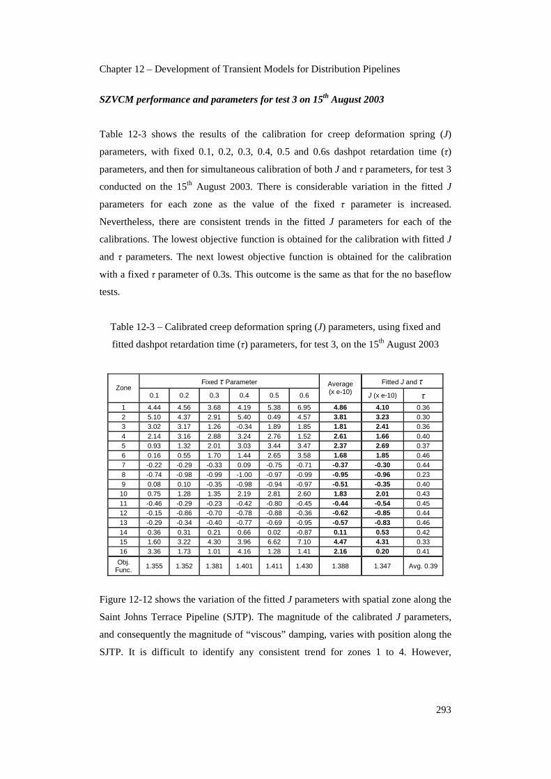
Chapter 12 – Development of Transient Models for Distribution Pipelines
293
SZVCM performance and parameters for test 3 on 15th August 2003
Table 12-3 shows the results of the calibration for creep deformation spring (J)
parameters, with fixed 0.1, 0.2, 0.3, 0.4, 0.5 and 0.6s dashpot retardation time (τ)
parameters, and then for simultaneous calibration of both J and τ parameters, for test 3
conducted on the 15th August 2003. There is considerable variation in the fitted J
parameters for each zone as the value of the fixed τ parameter is increased.
Nevertheless, there are consistent trends in the fitted J parameters for each of the
calibrations. The lowest objective function is obtained for the calibration with fitted J
and τ parameters. The next lowest objective function is obtained for the calibration
with a fixed τ parameter of 0.3s. This outcome is the same as that for the no baseflow
tests.
Table 12-3 – Calibrated creep deformation spring (J) parameters, using fixed and
fitted dashpot retardation time (τ) parameters, for test 3, on the 15th August 2003
Fixed τ Parameter Fitted J and τZone
0.1 0.2 0.3 0.4 0.5 0.6
Average (x e-10) J (x e-10) τ
1 4.44 4.56 3.68 4.19 5.38 6.95 4.86 4.10 0.36 2 5.10 4.37 2.91 5.40 0.49 4.57 3.81 3.23 0.30 3 3.02 3.17 1.26 -0.34 1.89 1.85 1.81 2.41 0.36 4 2.14 3.16 2.88 3.24 2.76 1.52 2.61 1.66 0.40 5 0.93 1.32 2.01 3.03 3.44 3.47 2.37 2.69 0.37 6 0.16 0.55 1.70 1.44 2.65 3.58 1.68 1.85 0.46 7 -0.22 -0.29 -0.33 0.09 -0.75 -0.71 -0.37 -0.30 0.44 8 -0.74 -0.98 -0.99 -1.00 -0.97 -0.99 -0.95 -0.96 0.23 9 0.08 0.10 -0.35 -0.98 -0.94 -0.97 -0.51 -0.35 0.40
10 0.75 1.28 1.35 2.19 2.81 2.60 1.83 2.01 0.43 11 -0.46 -0.29 -0.23 -0.42 -0.80 -0.45 -0.44 -0.54 0.45 12 -0.15 -0.86 -0.70 -0.78 -0.88 -0.36 -0.62 -0.85 0.44 13 -0.29 -0.34 -0.40 -0.77 -0.69 -0.95 -0.57 -0.83 0.46 14 0.36 0.31 0.21 0.66 0.02 -0.87 0.11 0.53 0.42 15 1.60 3.22 4.30 3.96 6.62 7.10 4.47 4.31 0.33 16 3.36 1.73 1.01 4.16 1.28 1.41 2.16 0.20 0.41
Obj. Func. 1.355 1.352 1.381 1.401 1.411 1.430 1.388 1.347 Avg. 0.39
Figure 12-12 shows the variation of the fitted J parameters with spatial zone along the
Saint Johns Terrace Pipeline (SJTP). The magnitude of the calibrated J parameters,
and consequently the magnitude of “viscous” damping, varies with position along the
SJTP. It is difficult to identify any consistent trend for zones 1 to 4. However,

Chapter 12 – Development of Transient Models for Distribution Pipelines
294
consistent trends are evident, despite variations in magnitude, for zones 7 to 16. The
trends for zones 5 to 6 are less consistent than for the tests without baseflow.
-2
-1
0
1
2
3
4
5
6
7
8
1 2 3 4 5 6 7 8 9 10 11 12 13 14 15 16Zone
Fit
ted
Par
amet
er J
(P
a-1)
x e-
10 Tau = 0.1 Tau = 0.2 Tau = 0.3 Tau = 0.4
Tau = 0.5 Tau = 0.6 Average Tau Fitted Tau
Figure 12-12 – Fitted J parameters for test 3, conducted on the 15th August 2003, with
baseflow, for fixed and fitted τ parameter calibrations
Table 12-4 – J parameter correlations for different zones for test 3
J1 J2 J3 J4 J5 J6 J7 J8 J9 J10 J11 J12 J13 J14 J15 J16
J1 1.00 0.21 0.03 0.01 0.28 0.01 0.19 0.01 0.20 0.06 0.26 0.02 0.13 0.10 0.17 0.04
J2 0.21 1.00 0.04 0.39 0.45 0.14 0.00 0.28 0.01 0.06 0.42 0.39 0.06 0.72 0.04 0.39
J3 0.03 0.04 1.00 0.80 0.01 0.02 0.48 0.02 0.36 0.39 0.37 0.79 0.98 0.05 0.50 0.34
J4 0.01 0.39 0.80 1.00 0.42 0.03 0.19 0.21 0.09 0.29 0.63 0.99 0.83 0.48 0.15 0.13
J5 0.28 0.45 0.01 0.42 1.00 0.12 0.01 0.33 0.03 0.13 0.86 0.48 0.01 0.57 0.06 0.43
J6 0.01 0.14 0.02 0.03 0.12 1.00 0.41 0.06 0.41 0.79 0.09 0.06 0.03 0.17 0.28 0.53
J7 0.19 0.00 0.48 0.19 0.01 0.41 1.00 0.04 0.94 0.08 0.36 0.27 0.42 0.12 0.84 0.74
J8 0.01 0.28 0.02 0.21 0.33 0.06 0.04 1.00 0.20 0.06 0.22 0.21 0.02 0.39 0.08 0.35
J9 0.20 0.01 0.36 0.09 0.03 0.41 0.94 0.20 1.00 0.21 0.35 0.19 0.30 0.10 0.88 0.76
J10 0.06 0.06 0.39 0.29 0.13 0.79 0.08 0.06 0.21 1.00 0.12 0.20 0.30 0.00 0.16 0.30
J11 0.26 0.42 0.37 0.63 0.86 0.09 0.36 0.22 0.35 0.12 1.00 0.70 0.33 0.49 0.22 0.17
J12 0.02 0.39 0.79 0.99 0.48 0.06 0.27 0.21 0.19 0.20 0.70 1.00 0.83 0.49 0.22 0.08
J13 0.13 0.06 0.98 0.83 0.01 0.03 0.42 0.02 0.30 0.30 0.33 0.83 1.00 0.01 0.47 0.31
J14 0.10 0.72 0.05 0.48 0.57 0.17 0.12 0.39 0.10 0.00 0.49 0.49 0.01 1.00 0.19 0.60
J15 0.17 0.04 0.50 0.15 0.06 0.28 0.84 0.08 0.88 0.16 0.22 0.22 0.47 0.19 1.00 0.76
J16 0.04 0.39 0.34 0.13 0.43 0.53 0.74 0.35 0.76 0.30 0.17 0.08 0.31 0.60 0.76 1.00
Table 12-4 (above) shows the correlation of calibrated J parameters for the different
zones along the SJTP, when the τ parameters have been simultaneously fitted, for test
3, conducted on the 15th August 2003. Generally, the fitted J parameters for each of
the 16 zones are not highly correlated. As for the case without baseflow, the fitted τ

Chapter 12 – Development of Transient Models for Distribution Pipelines
295
parameters are neither highly correlated between zones nor with the fitted J
parameters.
Comparison of results from tests without and with baseflow
Figure 12-13 compares the calibrated J parameters, determined as an average of the
results for each fixed τ parameter, with the J parameters, calibrated while
simultaneously fitting for τ parameters, for test 2, conducted without baseflow on the
23rd July 2003, and test 3, conducted with baseflow on the 15th August 2003,
respectively. There is a marked divergence between the calibrated J parameters for
zones 1 to 6 for the tests conducted without and with baseflow. That said, the
calibrated J parameters are relatively similar for zones 7 to 16.
-2
-1
0
1
2
3
4
5
6
1 2 3 4 5 6 7 8 9 10 11 12 13 14 15 16Zone
Fit
ted
Par
amet
er J
(P
a-1)
x e-
10 Test 2 (23rd July) - Average Tau Test 3 (15th Aug) - Average Tau
Test 2 (23rd July) - Fitted Tau Test 3 (15th Aug) - Fitted Tau
Figure 12-13 – Comparison of fitted J parameters for test 2, conducted on the 23rd
July 2003, and for test 3, conducted on the 15th August 2003
It is possible that the difference for zones 1 to 6 is related to the reduction of pressure
along the Saint Johns Terrace Pipeline (SJTP) for test 3, with baseflow, and, in
particular, the reduction of pressure along the sections with higher elevations and less
static pressure. The “viscous” damping associated with mechanical motion and
vibration, flexible joints and soil/pipe interaction may, depending on the physical
processes involved, be greater if the SJTP is subject to less static pressure.

Chapter 12 – Development of Transient Models for Distribution Pipelines
296
Nevertheless, the consistency in the calibrated J parameters for zones 7 to 16 supports
the hypothesis that “viscous” damping can be used to replicate the effects of physical
complexity along at least part of the SJTP.
12.3.5 Assessment of lower number of spatial zones for SZVCM
While a spatially zoned “viscous” calibration model (SZVCM) with 16 zones has
been adopted for the calibration described above, a smaller number of spatial zones
may facilitate adequate replication of the effects of the physical variability, and
changes in the magnitude of “viscous” damping, along the Saint Johns Terrace
Pipeline (SJTP). In order to assess the sensitivity of the results to the number of
spatial zones, SZVCMs with 8 and 4 zones have been calibrated below.
The calibrations are performed using the measured response from test 2, conducted on
the 23rd July 2003, without baseflow. Given the general consistency of the calibrated J
and τ parameters obtained for this test with those obtained for the other tests, test 2
was considered sufficient to gauge the performance of the 8 and 4 zone SZVCMs.
Furthermore, it was considered sufficient to perform the calibration using only fitted,
and not fixed, τ parameters.
Assessment of 8 zone SZVCM
Figures 12-14 and 12-15 show the measured versus predicted responses for test 2
following calibration using a spatially zoned “viscous” calibration model (SZVCM)
with 8 zones, and fitted τ parameters, at stations 1 and 2, respectively. The predicted
responses obtained using the 16 zone SZVCM and traditional forward transient model
are plotted for comparison. There is a marked improvement relative to the predicted
results obtained when using a traditional forward transient model. Figures 12-16 and
12-17 show that the calibrated response obtained using the 8 zone SZVCM is
marginally less accurate than that obtained using the 16 zone SZVCM.

Chapter 12 – Development of Transient Models for Distribution Pipelines
297
26
29
32
35
38
41
0 0.1 0.2 0.3 0.4 0.5Time (s)
Pre
ssu
re (
m)
Measured response
Predicted response - 16 zones
Predicted response - 8 zones
Traditional model
33
36
39
42
45
48
0 0.1 0.2 0.3 0.4 0.5Time (s)
Pre
ssu
re (
m)
Measured response
Predicted response - 16 zones
Predicted response - 8 zones
Traditional model
Figures 12-14 and 12-15 – Measured and predicted responses, obtained using 16 and
8 zone SZVCMs, for test 2, at stations 1 and 2, respectively
33
34
35
36
37
38
39
0.10 0.18 0.26 0.34 0.42 0.50Time (s)
Pre
ssu
re (
m)
Measured response
Predicted response - 16 zones
Predicted response - 8 zones
40
41
42
43
44
45
46
0.00 0.10 0.20 0.30 0.40 0.50Time (s)
Pre
ssu
re (
m)
Measured response
Predicted response - 16 zones
Predicted response - 8 zones
Figures 12-16 and 12-17 – Measured and predicted responses, obtained using 16 and
8 zone SZVCMs, over a pressure range of 6m, at stations 1 and 2, respectively
The coefficients of determination for the measured and predicted responses are 98.4%
and 88.6%, for the calibrations performed using the 8 zone SZVCM, at stations 1 and
2, respectively (compared to 99.1% and 88.9% when calibrating using the 16 zone
SZVCM). These coefficients of determination indicate that the predicted responses
approximately replicate the measured responses. The coefficient of determination is
lower for station 2 because of the inaccuracies in the replication of the “ringing”
effect of the transient generator.
Figures 12-18 and 12-19 show the standardised residual plotted against time for test 2,
for the calibrations performed using the 16 and 8 zone SZVCMs, at stations 1 and 2,
respectively. Relative to the results obtained using the 16 zone SZVCM, marginally
longer “runs” of positive and negative residuals are obtained using the 8 zone
SZVCM. Variations in the standardised residual, associated with inadequacies in the

Chapter 12 – Development of Transient Models for Distribution Pipelines
298
replication of the “ringing” effect from the transient generator, are particularly
apparent for a short time following the induction of the transient at station 2.
-3
-2
-1
0
1
2
3
0 0.1 0.2 0.3 0.4 0.5
Time (s)
Sta
nd
ard
ised
res
idu
al
16 zones
8 zones
-3
-2
-1
0
1
2
3
0 0.1 0.2 0.3 0.4 0.5
Time (s)
Sta
nd
ard
ised
res
idu
al
16 zones
8 zones
Figures 12-18 and 12-19 – Standardised residual versus time plots, obtained using 16
and 8 zone SZVCMs, for test 2, at stations 1 and 2, respectively
Assessment of 4 zone SZVCM
Figures 12-20 and 12-21 show the measured versus predicted responses for test 2
following calibration using a spatially zoned “viscous” calibration model (SZVCM)
with 4 zones, and fitted τ parameters, at stations 1 and 2, respectively. There is a
marked improvement, relative to the predicted results obtained when using a
traditional forward transient model, when using the 4 zone SZVCM. However,
Figures 12-22 and 12-23 show that the calibrated response obtained using the 4 zone
SZVCM is significantly less accurate than that obtained using the 16 zone SZVCM
(and 8 zone SZVCM).
26
29
32
35
38
41
0 0.1 0.2 0.3 0.4 0.5Time (s)
Pre
ssu
re (
m)
Measured response
Predicted response - 16 zones
Predicted response - 4 zones
Traditional model
33
36
39
42
45
48
0 0.1 0.2 0.3 0.4 0.5Time (s)
Pre
ssu
re (
m)
Measured response
Predicted response - 16 zones
Predicted response - 4 zones
Traditional model
Figures 12-20 and 12-21 – Measured and predicted responses, obtained using 16 and
4 zone SZVCMs, for test 2, at stations 1 and 2, respectively

Chapter 12 – Development of Transient Models for Distribution Pipelines
299
33
34
35
36
37
38
39
0.10 0.18 0.26 0.34 0.42 0.50Time (s)
Pre
ssu
re (
m)
Measured response
Predicted response - 16 zones
Predicted response - 4 zones
40
41
42
43
44
45
46
0.00 0.10 0.20 0.30 0.40 0.50Time (s)
Pre
ssu
re (
m)
Measured response
Predicted response - 16 zones
Predicted response - 4 zones
Figures 12-22 and 12-23 – Measured and predicted responses, obtained using 16 and
4 zone SZVCMs, over a pressure range of 6m, at stations 1 and 2, respectively
The coefficients of determination for the measured and predicted responses are 97.1%
and 84.1%, for the calibrations performed using the 4 zone SZVCM, at stations 1 and
2, respectively (compared to 99.1% and 88.9% when calibrating using the 16 zone
SZVCM). The loss of accuracy relative to the results obtained using the 16 and 8 zone
SZVCMs is significant.
Figures 12-24 and 12-25 show the standardised residual plotted against time for test 2,
for the calibrations performed using the 8 and 4 zone SZVCMs, at stations 1 and 2,
respectively. Relative to the results obtained using the 8 zone SZVCM, significantly
longer “runs” of positive and negative residuals are obtained using the 4 zone
SZVCM. This confirms that the error for the 4 zone SZVCM is less random than for
the 8 and 16 zone SZVCMs.
-3
-2
-1
0
1
2
3
0 0.1 0.2 0.3 0.4 0.5
Time (s)
Sta
nd
ard
ised
res
idu
al
8 zones
4 zones
-3
-2
-1
0
1
2
3
0 0.1 0.2 0.3 0.4 0.5
Time (s)
Sta
nd
ard
ised
res
idu
al
8 zones
4 zones
Figures 12-24 and 12-25 – Standardised residual versus time plots, obtained using 8
and 4 zone SZVCMs, for test 2, at stations 1 and 2, respectively

Chapter 12 – Development of Transient Models for Distribution Pipelines
300
Parameter correlations for the 8 and 4 zone SZVCMs
Table 12-5 shows the correlation of calibrated J and τ parameters, for the different
zones along the Saint Johns Terrace Pipeline (SJTP), obtained using the spatially
zoned “viscous” calibration model (SZVCM) with 8 zones, for test 2. Generally, the
fitted J and τ parameters for each of the 8 zones are not highly correlated. The general
lack of correlation between the fitted J parameters suggests that the 8 zone SZVCM is
not over-parameterised. Table 12-6 shows the correlation of calibrated J and τ
parameters, for the different zones along the SJTP, obtained using the 4 zone
SZVCM, for test 2. The fitted J and τ parameters for each of the for zones are, again,
not generally highly correlated.
Table 12-5 – J and τ parameter correlations for 8 zone SZVCM for test 2
J1 τ1 J2 τ2 J3 τ3 J4 τ4 J5 τ5 J6 τ6 J7 τ7 J8 τ8
J1 1.00 0.98 0.01 0.09 0.18 0.24 0.21 0.21 0.21 0.20 0.09 0.04 0.15 0.21 0.07 0.06
τ1 0.98 1.00 0.19 0.12 0.08 0.13 0.19 0.19 0.18 0.16 0.07 0.03 0.13 0.20 0.07 0.06
J2 0.01 0.19 1.00 0.97 0.13 0.10 0.08 0.07 0.13 0.18 0.26 0.21 0.19 0.02 0.06 0.06
τ2 0.09 0.12 0.97 1.00 0.31 0.30 0.06 0.06 0.11 0.16 0.22 0.18 0.18 0.00 0.05 0.05
J3 0.18 0.08 0.13 0.31 1.00 0.98 0.51 0.52 0.48 0.46 0.01 0.12 0.03 0.01 0.19 0.18
τ3 0.24 0.13 0.10 0.30 0.98 1.00 0.35 0.37 0.37 0.37 0.06 0.03 0.00 0.00 0.11 0.11
J4 0.21 0.19 0.08 0.06 0.51 0.35 1.00 1.00 0.86 0.77 0.20 0.39 0.16 0.06 0.40 0.37
τ4 0.21 0.19 0.07 0.06 0.52 0.37 1.00 1.00 0.87 0.78 0.18 0.37 0.15 0.06 0.39 0.36
J5 0.21 0.18 0.13 0.11 0.48 0.37 0.86 0.87 1.00 0.99 0.27 0.06 0.17 0.23 0.30 0.28
τ5 0.20 0.16 0.18 0.16 0.46 0.37 0.77 0.78 0.99 1.00 0.42 0.21 0.28 0.29 0.25 0.23
J6 0.09 0.07 0.26 0.22 0.01 0.06 0.20 0.18 0.27 0.42 1.00 0.97 0.80 0.58 0.22 0.20
τ6 0.04 0.03 0.21 0.18 0.12 0.03 0.39 0.37 0.06 0.21 0.97 1.00 0.77 0.55 0.30 0.28
J7 0.15 0.13 0.19 0.18 0.03 0.00 0.16 0.15 0.17 0.28 0.80 0.77 1.00 0.91 0.14 0.15
τ7 0.21 0.20 0.02 0.00 0.01 0.00 0.06 0.06 0.23 0.29 0.58 0.55 0.91 1.00 0.02 0.04
J8 0.07 0.07 0.06 0.05 0.19 0.11 0.40 0.39 0.30 0.25 0.22 0.30 0.14 0.02 1.00 1.00
τ8 0.06 0.06 0.06 0.05 0.18 0.11 0.37 0.36 0.28 0.23 0.20 0.28 0.15 0.04 1.00 1.00
Table 12-6 – J and τ correlations for 4 zone SZVCM for test 2
J1 τ1 J2 τ2 J3 τ3 J4 τ4
J1 1.00 0.58 0.88 0.88 0.41 0.38 0.04 0.03
τ1 0.58 1.00 0.38 0.39 0.17 0.14 0.01 0.00
J2 0.88 0.38 1.00 1.00 0.74 0.69 0.20 0.17
τ2 0.88 0.39 1.00 1.00 0.73 0.69 0.22 0.19
J3 0.41 0.17 0.74 0.73 1.00 0.97 0.38 0.34
τ3 0.38 0.14 0.69 0.69 0.97 1.00 0.49 0.46
J4 0.04 0.01 0.20 0.22 0.38 0.49 1.00 1.00
τ4 0.03 0.00 0.17 0.19 0.34 0.46 1.00 1.00

Chapter 12 – Development of Transient Models for Distribution Pipelines
301
Performance of the 16, 8 and 4 zone SZVCMs
Table 12-7 shows the results of the calibration for creep deformation spring (J) and
dashpot retardation time (τ) parameters for test 2, using spatially zoned “viscous”
calibration models (SZVCMs) with 16, 8 and 4 zones. The objective functions
obtained for the calibrations are 1.83, 2.22 and 3.07, respectively. On the basis of
lowest objective function, and an assessment of the regression diagnostics, the 16
zone SZVCM is superior to the 8 and 4 zone SZVCMs. Furthermore, the parameter
correlations for the 16 zone SZVCM indicate that it is not over-parameterised.
Table 12-7 – Calibrated creep deformation spring (J) and dashpot retardation time (τ)
parameters for test 2 using 16, 8 and 4 zone SZVCMs
Number of spatial zones in model
16 8 4 Zone
Fitted J (x e-10) Pa-1
Fitted τ(s)
Fitted J (x e-10) Pa-1
Fitted τ(s)
Fitted J (x e-10) Pa-1
Fitted τ(s)
1 3.94 0.37 1.29 0.43 0.20 0.05 2 1.14 0.40 0.21 0.31 0.60 0.65 3 1.27 0.56 0.65 0.36 0.30 0.26 4 0.31 0.46 -0.76 0.46 1.14 0.65 5 0.95 0.35 2.72 0.60 NA NA 6 0.46 0.39 -0.41 0.43 NA NA 7 0.14 0.39 -0.24 0.25 NA NA 8 -0.69 0.37 2.31 0.54 NA NA 9 0.14 0.39 NA NA NA NA 10 2.35 0.29 NA NA NA NA 11 -0.24 0.54 NA NA NA NA 12 -0.98 0.40 NA NA NA NA 13 -1.00 0.41 NA NA NA NA 14 1.55 0.40 NA NA NA NA 15 3.21 0.41 NA NA NA NA 16 -0.36 0.48 NA NA NA NA
1.83 Obj Func Avg. 0.42 2.22 Obj Func Avg. 0.41 3.07 Obj Func Avg. 0.40
Figure 12-26 shows the variation of the fitted J parameters with spatial zone along the
Saint Johns Terrace Pipeline (SJTP), for calibrations obtained for test 2 using the 16
and 8 zone SZVCMs. Despite halving the number of zones, the magnitudes of the
calibrated J parameters, and consequently the magnitude of “viscous” damping, are
relatively consistent along the SJTP for both models. This suggests that the 8 zone
SZVCM is sufficiently flexible, in terms of representing variations in the physical
complexities that disperse and damp the response of the SJTP, to be relatively
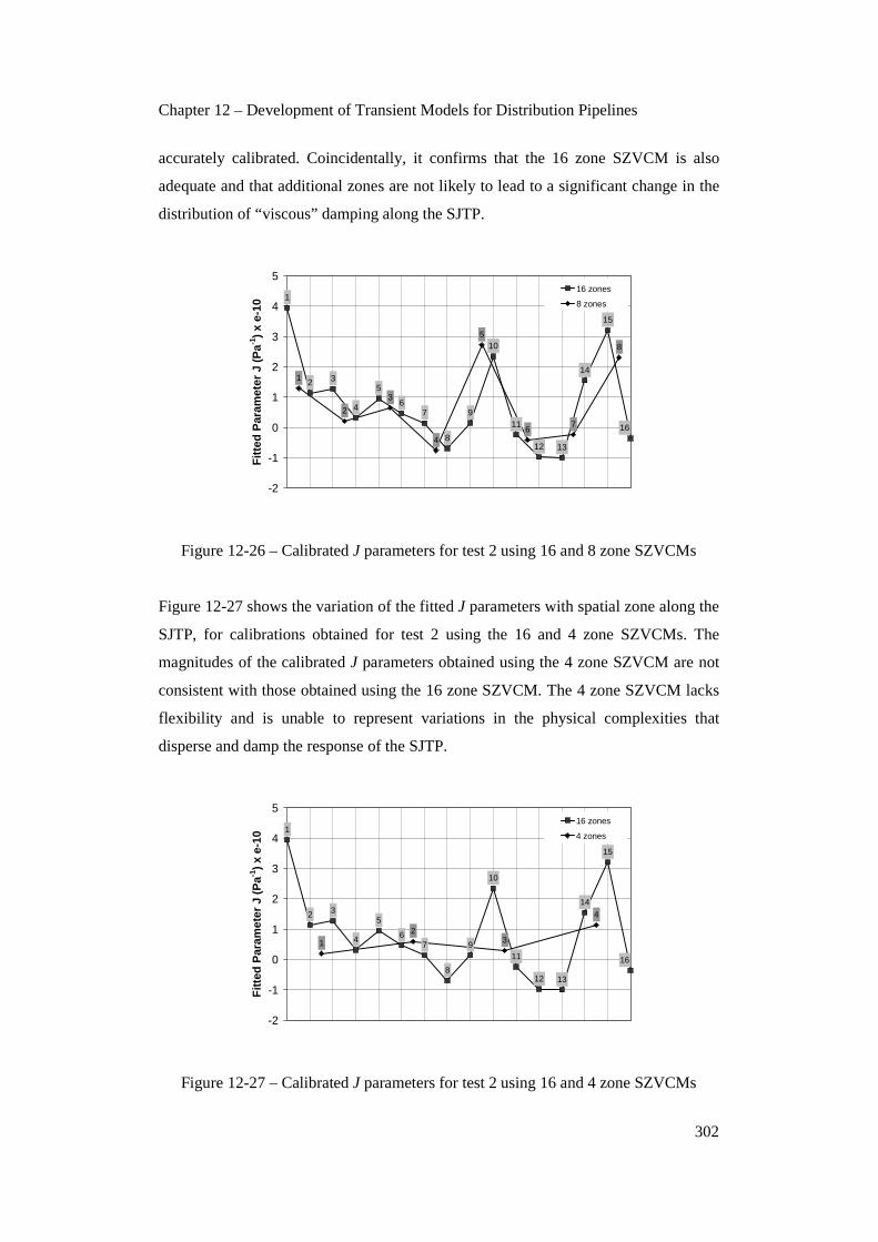
Chapter 12 – Development of Transient Models for Distribution Pipelines
302
accurately calibrated. Coincidentally, it confirms that the 16 zone SZVCM is also
adequate and that additional zones are not likely to lead to a significant change in the
distribution of “viscous” damping along the SJTP.
7
8
9
10
11
12 13
14
15
16
6
53
1
2
4
8
76
5
4
3
1
2
-2
-1
0
1
2
3
4
5
Fit
ted
Par
amet
er J
(P
a-1)
x e-
10
16 zones
8 zones
Figure 12-26 – Calibrated J parameters for test 2 using 16 and 8 zone SZVCMs
Figure 12-27 shows the variation of the fitted J parameters with spatial zone along the
SJTP, for calibrations obtained for test 2 using the 16 and 4 zone SZVCMs. The
magnitudes of the calibrated J parameters obtained using the 4 zone SZVCM are not
consistent with those obtained using the 16 zone SZVCM. The 4 zone SZVCM lacks
flexibility and is unable to represent variations in the physical complexities that
disperse and damp the response of the SJTP.
7
8
9
10
11
12 13
14
15
16
6
53
1
2
4
4
32
1
-2
-1
0
1
2
3
4
5
Fit
ted
Par
amet
er J
(P
a-1)
x e-
10
16 zones
4 zones
Figure 12-27 – Calibrated J parameters for test 2 using 16 and 4 zone SZVCMs

Chapter 12 – Development of Transient Models for Distribution Pipelines
303
12.4 Calibration of spatially zoned model of the KCP
12.4.1 Description of the spatially zoned “viscous” model
The number of spatial zones, and hence Kelvin-Voigt elements, along the Kookaburra
Court Pipeline (KCP) is initially set to 8 because the KCP is shorter than the Saint
Johns Terrace Pipeline (SJTP). This gives 16 Kevin-Voigt parameters (i.e., 8 creep
deformation spring (J) and 8 dashpot retardation time (τ) parameters). Figure 12-28
shows a schematic of the KCP with 8 spatial zones each 47.3m long (i.e.,
approximately 40 by 1.18m sub-pipe segments long).
84 5 61 2 3 7
Fire plug - typical “Transient Generator”
Artificial air pocket Artificial leak
8 spatial zones x 47.3m long each
Figure 12-28 – Kookaburra Court Pipeline divided into spatial zones for calibration
using 8 pairs of Kelvin-Voigt spring and dashpot parameters
Pairs of creep deformation spring and dashpot retardation time parameters are
separately calibrated to replicate the dispersive and damping effect of mechanical
motion and vibration, flexible joints and soil/pipe interaction within each zone.
Calibration is performed using the measured responses for test 3, conducted on the
28th August 2003, from stations 1 and 2. Calibration using fixed τ parameters is
performed to assess the sensitivity of the calibration to these parameters. The results
are presented with those obtained when simultaneously calibrating the τ parameters.

Chapter 12 – Development of Transient Models for Distribution Pipelines
304
It was not possible to accurately determine either the topology or physical condition
of the 15 water service connections along the KCP (this scenario is likely to be typical
of the general situation for other distribution pipelines). A complex forward transient
model of the KCP, as described in Chapter 11, has been developed and includes 15 by
10m long branches of 25mm pipe, with 20mm orifices for individual water meters,
located approximately 3.5m along each offtake (measured from the KCP),
representing each water service connection.
While the size of the offtakes and location of the water meters are topologically
correct, the approximation of each water service connection, using a 10m length of
pipe, is likely to be deficient. Given this uncertainty, a topologically simplified
forward transient model has been developed (excluding the 10m lengths of pipe used
to approximate each water service connection). The results of the calibration of a
spatially zoned “viscous” calibration model (SZVCM) with 8 zones, and simplified
topology, will be compared with those obtained using a complex topology.
12.4.2 Calibration of complex spatially zoned “viscous” model
Figures 12-29 and 12-30 show the measured versus predicted responses for test 3,
conducted on the 28th August 2003, following calibration using a topologically
complex spatially zoned “viscous” calibration model (SZVCM) with 8 zones, at
stations 1 and 2, respectively. Only a proportion of the measured and predicted
reflections correlate with each other. Given the uncertainty in the topology, condition
and anticipated response of the water service connections, this result is not
unexpected. The coefficients of determination for the measured and predicted
responses are 99.6% and 98.3% at stations 1 and 2, respectively. The coefficient of
determination is lower for station 2 because of inaccuracies in the replication of the
“ringing” effect of the transient generator.
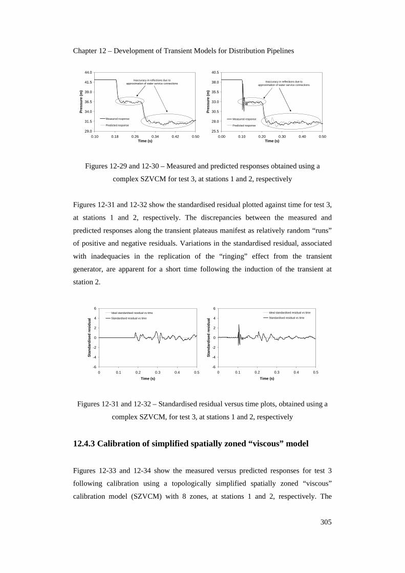
Chapter 12 – Development of Transient Models for Distribution Pipelines
305
29.0
31.5
34.0
36.5
39.0
41.5
44.0
0.10 0.18 0.26 0.34 0.42 0.50Time (s)
Pre
ssu
re (
m)
Measured response
Predicted response
Inaccuracy in reflections due to approximation of water service connections
25.5
28.0
30.5
33.0
35.5
38.0
40.5
0.00 0.10 0.20 0.30 0.40 0.50Time (s)
Pre
ssu
re (
m)
Measured response
Predicted response
Inaccuracy in reflections due to approximation of water service connections
Figures 12-29 and 12-30 – Measured and predicted responses obtained using a
complex SZVCM for test 3, at stations 1 and 2, respectively
Figures 12-31 and 12-32 show the standardised residual plotted against time for test 3,
at stations 1 and 2, respectively. The discrepancies between the measured and
predicted responses along the transient plateaus manifest as relatively random “runs”
of positive and negative residuals. Variations in the standardised residual, associated
with inadequacies in the replication of the “ringing” effect from the transient
generator, are apparent for a short time following the induction of the transient at
station 2.
-6
-4
-2
0
2
4
6
0 0.1 0.2 0.3 0.4 0.5
Time (s)
Sta
nd
ard
ised
res
idu
al
Ideal standardised residual vs time
Standardised residual vs time
-6
-4
-2
0
2
4
6
0 0.1 0.2 0.3 0.4 0.5
Time (s)
Sta
nd
ard
ised
res
idu
al
Ideal standardised residual vs time
Standardised residual vs time
Figures 12-31 and 12-32 – Standardised residual versus time plots, obtained using a
complex SZVCM, for test 3, at stations 1 and 2, respectively
12.4.3 Calibration of simplified spatially zoned “viscous” model
Figures 12-33 and 12-34 show the measured versus predicted responses for test 3
following calibration using a topologically simplified spatially zoned “viscous”
calibration model (SZVCM) with 8 zones, at stations 1 and 2, respectively. The

Chapter 12 – Development of Transient Models for Distribution Pipelines
306
calibrated responses obtained using the simplified SZVCM are devoid of reflections
apart from those from the vertical fire plug risers (which are retained in the simplified
model). This confirms that the water service connections (as approximated) affect the
predicted responses of the KCP. The coefficients of determination for the measured
and predicted responses are 99.1% and 98.0% at stations 1 and 2, respectively
(compared to 99.6% and 98.3% when calibrating using the complex SZVCM).
29.0
31.5
34.0
36.5
39.0
41.5
44.0
0.10 0.18 0.26 0.34 0.42 0.50Time (s)
Pre
ssu
re (
m)
Measured response
Predicted response
Water services (as approximated) excluded in simplified model
25.5
28.0
30.5
33.0
35.5
38.0
40.5
0.00 0.10 0.20 0.30 0.40 0.50Time (s)
Pre
ssu
re (
m)
Measured response
Predicted response
Water services (as approximated) excluded in simplified model
Figures 12-33 and 12-34 – Measured and predicted responses obtained using a
simplified SZVCM for test 3, at stations 1 and 2, respectively
Figures 12-35 and 12-36 show the standardised residual plotted against time for test 3,
at stations 1 and 2, respectively. The discrepancies between the measured and
predicted responses along the transient plateaus manifest as “runs” of positive and
negative residuals. These “runs” are significantly longer than for the results obtained
using the complex SZVCM.
-6
-4
-2
0
2
4
6
0 0.1 0.2 0.3 0.4 0.5
Time (s)
Sta
nd
ard
ised
res
idu
al
Ideal standardised residual vs time
Standardised residual vs time
-6
-4
-2
0
2
4
6
0 0.1 0.2 0.3 0.4 0.5
Time (s)
Sta
nd
ard
ised
res
idu
al
Ideal standardised residual vs time
Standardised residual vs time
Figures 12-35 and 12-36 – Standardised residual versus time plots, obtained using a
simplified SZVCM, for test 3, at stations 1 and 2, respectively

Chapter 12 – Development of Transient Models for Distribution Pipelines
307
12.4.4 Assessment of SZVCM and parameterisation
Complex SZVCM performance and parameters
Table 12-8 shows the results of the calibration, using a topologically complex
spatially zoned “viscous” calibration model (SZVCM) with 8 zones, of creep
deformation spring (J) parameters, with fixed 0.1, 0.2, 0.3, 0.4, 0.5 and 0.6s dashpot
retardation time (τ) parameters, and then simultaneous calibration of both J and τ
parameters. There is considerable variation in the fitted J parameters for each zone as
the value of the fixed τ parameter is increased. Nevertheless, there are consistent
trends in the fitted J parameters. The lowest objective function is obtained for the
calibration with fitted J and τ parameters. The next lowest objective function is
obtained for the calibration with a fixed τ parameter of 0.3s.
Table 12-8 – Calibrated creep deformation spring (J) parameters, using fixed and
fitted dashpot retardation time (τ) parameters, for test 3
Fixed Tau Parameter Fitted J and Tau Zone
0.1 0.2 0.3 0.4 0.5 0.6
Average (x e-10) J (x e-10) Tau
1 4.30 8.02 9.95 5.73 9.98 8.21 7.70 3.99 0.39 2 -0.05 0.09 0.30 0.47 0.80 1.08 0.45 0.25 0.39 3 -0.11 -0.20 -0.35 -0.34 -0.62 -0.80 -0.40 -0.23 0.43 4 -0.07 -0.03 -0.09 -0.05 0.11 0.15 0.00 0.01 0.37 5 -0.14 -0.25 -0.06 -0.32 -0.36 -0.37 -0.25 -0.40 0.43 6 0.11 0.24 -0.06 0.37 0.31 0.22 0.20 0.44 0.36 7 -0.35 -0.53 -0.72 -0.83 -1.00 -1.00 -0.74 -0.99 0.44 8 0.14 0.17 0.29 0.21 0.29 0.26 0.23 0.17 0.27
Obj. Func. 0.452 0.443 0.439 0.481 0.468 0.470 0.459 0.434 Avg. 0.39
Figure 12-37 shows the variation of the fitted J parameters with spatial zone along the
Kookaburra Court Pipeline (KCP). The magnitude of the calibrated J parameters, and
consequently the magnitude of “viscous” damping, varies with position along the
KCP. These variations in magnitude appear to be correlated with changes in the fixed
τ parameter. Figure 12-38 shows the variation of the J parameters over a scale of
±1.0e-10Pa-1 for zones 2 to 8. The fitted J parameters for zones 3, 5 and 7, are
negative. It is difficult to physically interpret this result. The SZVCM is designed to
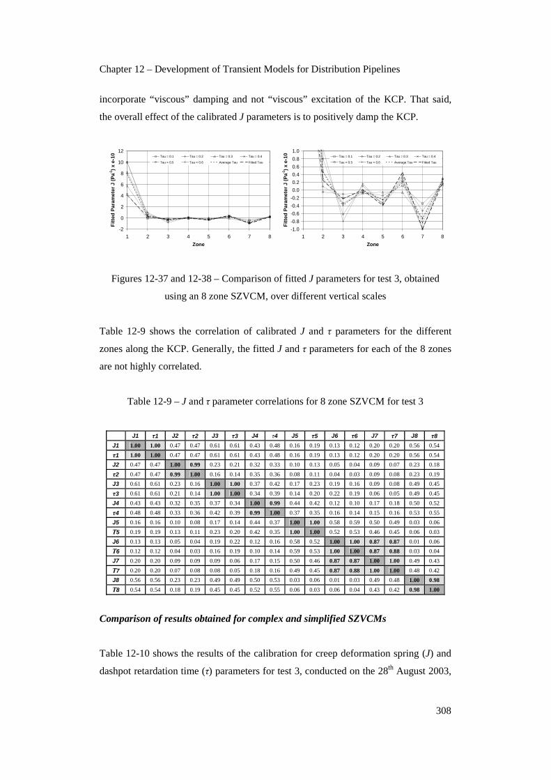
Chapter 12 – Development of Transient Models for Distribution Pipelines
308
incorporate “viscous” damping and not “viscous” excitation of the KCP. That said,
the overall effect of the calibrated J parameters is to positively damp the KCP.
-2
0
2
4
6
8
10
12
1 2 3 4 5 6 7 8
Zone
Fit
ted
Par
amet
er J
(P
a-1)
x e-
10 Tau = 0.1 Tau = 0.2 Tau = 0.3 Tau = 0.4
Tau = 0.5 Tau = 0.6 Average Tau Fitted Tau
-1.0
-0.8
-0.6
-0.4
-0.2
0.0
0.2
0.4
0.6
0.8
1.0
1 2 3 4 5 6 7 8
Zone
Fit
ted
Par
amet
er J
(P
a-1)
x e-
10 Tau = 0.1 Tau = 0.2 Tau = 0.3 Tau = 0.4
Tau = 0.5 Tau = 0.6 Average Tau Fitted Tau
Figures 12-37 and 12-38 – Comparison of fitted J parameters for test 3, obtained
using an 8 zone SZVCM, over different vertical scales
Table 12-9 shows the correlation of calibrated J and τ parameters for the different
zones along the KCP. Generally, the fitted J and τ parameters for each of the 8 zones
are not highly correlated.
Table 12-9 – J and τ parameter correlations for 8 zone SZVCM for test 3
J1 τ1 J2 τ2 J3 τ3 J4 τ4 J5 τ5 J6 τ6 J7 τ7 J8 τ8
J1 1.00 1.00 0.47 0.47 0.61 0.61 0.43 0.48 0.16 0.19 0.13 0.12 0.20 0.20 0.56 0.54
τ1 1.00 1.00 0.47 0.47 0.61 0.61 0.43 0.48 0.16 0.19 0.13 0.12 0.20 0.20 0.56 0.54
J2 0.47 0.47 1.00 0.99 0.23 0.21 0.32 0.33 0.10 0.13 0.05 0.04 0.09 0.07 0.23 0.18
τ2 0.47 0.47 0.99 1.00 0.16 0.14 0.35 0.36 0.08 0.11 0.04 0.03 0.09 0.08 0.23 0.19
J3 0.61 0.61 0.23 0.16 1.00 1.00 0.37 0.42 0.17 0.23 0.19 0.16 0.09 0.08 0.49 0.45
τ3 0.61 0.61 0.21 0.14 1.00 1.00 0.34 0.39 0.14 0.20 0.22 0.19 0.06 0.05 0.49 0.45
J4 0.43 0.43 0.32 0.35 0.37 0.34 1.00 0.99 0.44 0.42 0.12 0.10 0.17 0.18 0.50 0.52
τ4 0.48 0.48 0.33 0.36 0.42 0.39 0.99 1.00 0.37 0.35 0.16 0.14 0.15 0.16 0.53 0.55
J5 0.16 0.16 0.10 0.08 0.17 0.14 0.44 0.37 1.00 1.00 0.58 0.59 0.50 0.49 0.03 0.06
Τ5 0.19 0.19 0.13 0.11 0.23 0.20 0.42 0.35 1.00 1.00 0.52 0.53 0.46 0.45 0.06 0.03
J6 0.13 0.13 0.05 0.04 0.19 0.22 0.12 0.16 0.58 0.52 1.00 1.00 0.87 0.87 0.01 0.06
Τ6 0.12 0.12 0.04 0.03 0.16 0.19 0.10 0.14 0.59 0.53 1.00 1.00 0.87 0.88 0.03 0.04
J7 0.20 0.20 0.09 0.09 0.09 0.06 0.17 0.15 0.50 0.46 0.87 0.87 1.00 1.00 0.49 0.43
Τ7 0.20 0.20 0.07 0.08 0.08 0.05 0.18 0.16 0.49 0.45 0.87 0.88 1.00 1.00 0.48 0.42
J8 0.56 0.56 0.23 0.23 0.49 0.49 0.50 0.53 0.03 0.06 0.01 0.03 0.49 0.48 1.00 0.98
Τ8 0.54 0.54 0.18 0.19 0.45 0.45 0.52 0.55 0.06 0.03 0.06 0.04 0.43 0.42 0.98 1.00
Comparison of results obtained for complex and simplified SZVCMs
Table 12-10 shows the results of the calibration for creep deformation spring (J) and
dashpot retardation time (τ) parameters for test 3, conducted on the 28th August 2003,

Chapter 12 – Development of Transient Models for Distribution Pipelines
309
using topologically complex and simplified spatially zoned “viscous” calibration
models (SZVCMs) with 8 zones. The objective functions are 0.43 and 0.64 for the
calibration of the complex and simplified SZVCMs, respectively. On the basis of
lowest objective function, and an assessment of the regression diagnostics, the
SZVCM with complex topology is marginally superior.
Table 12-10 – Calibrated creep deformation spring (J) and dashpot retardation time (τ)
parameters using 8 zone SZVCMs with complex and simplified topologies
Fitted J and τ – complex topology Fitted J and τ – simplified topology Zone
J (x e-10) τ J (x e-10) τ
1 3.99 0.39 -0.24 0.43 2 0.25 0.39 0.60 0.31 3 -0.23 0.43 -0.75 0.40 4 0.01 0.37 -0.06 0.53 5 -0.40 0.43 -0.25 0.47 6 0.44 0.36 0.46 0.35 7 -0.99 0.44 -0.95 0.25 8 0.17 0.27 0.42 0.22
Obj. Func. 0.434 Avg. 0.39 0.638 Avg. 0.37
Figure 12-39 shows the variation of the fitted J parameters with spatial zone along the
Kookaburra Court Pipeline (KCP), when both J and τ parameters are simultaneously
calibrated using the complex and simplified 8 zone SZVCMs. Relatively consistent J
parameters are obtained for each of the zones, except for zone 1, regardless of
whether the model with complex or simplified topology is used. Figure 12-40 shows
the variation of the J parameters, over a scale of ±1.0e-10Pa-1, for zones 1 to 8.
-2
-1
0
1
2
3
4
5
1 2 3 4 5 6 7 8
Zone
Fit
ted
Par
amet
er J
(P
a-1)
x e-
10 Fitted Tau - complex FTM Fitted Tau - simplified FTM
-1.0
-0.8
-0.6
-0.4
-0.2
0.0
0.2
0.4
0.6
0.8
1.0
1 2 3 4 5 6 7 8
Zone
Fit
ted
Par
amet
er J
(P
a-1)
x e-
10 Fitted Tau - complex FTM Fitted Tau - simplified FTM
Figures 12-39 and 12-40 – Comparison of fitted J parameters obtained using 8 zone
SZVCMs, with complex and simplified topologies, over different vertical scales

Chapter 12 – Development of Transient Models for Distribution Pipelines
310
The consistency in the calibrated J parameters may be explained if the effects of
mechanical motion or vibration, flexible joints and soil/pipe interaction, rather than
the topology and physical condition of the water service connections, dominate the
“viscous” damping. Alternatively, the damping effects of the water service
connections may be being incorporated during the calibration. Both interpretations
suggest that the inclusion of the precise physical details of the water service
connections may not be significant for damping calibration.
That said, the use of the model with simplified topology leads to the omission of
significant reflections. Figures 12-41 and 12-42 show the standardised residual plotted
against time for test 3, for the calibrations performed using the complex and
simplified 8 zone SZVCMs with fitted τ parameters, at stations 1 and 2, respectively.
Relative to the results obtained using the complex model, marginally longer “runs” of
positive and negative residuals are obtained.
The neglect of the water service connections leads to the predicted wavefront pre-
empting the arrival of the measured reflected wavefront from the dead end of the KCP
(this manifests as the distinctive spike at both stations 1 and 2). Each water service
connection acts as a volumetric accumulator and their omission from a model will
result in predicted wavefronts arriving earlier than measured wavefronts. This
observation is important when the time of arrival of a wavefront at a station is used to
determine wave speed and/or infer the condition of the wall of a distribution pipeline.
-4
-3
-2
-1
0
1
2
3
4
0 0.1 0.2 0.3 0.4 0.5
Time (s)
Sta
nd
ard
ised
res
idu
al
Complex
Simplified
-4
-3
-2
-1
0
1
2
3
4
0 0.1 0.2 0.3 0.4 0.5
Time (s)
Sta
nd
ard
ised
res
idu
al
Complex
Simplified
Figures 12-41 and 12-42 – Standardised residual versus time plots, obtained using
SZVCMs with complex and simplified topologies, at stations 1 and 2, respectively

Chapter 12 – Development of Transient Models for Distribution Pipelines
311
That said, it has been presumed that the inclusion of more information regarding the
topology and condition of the water service connections will result in reflections
being accurately predicted. This is only true if the information is accurate. The
amount of physical information that can be gathered for any particular distribution
pipeline will vary significantly and, in some cases, no information regarding the
position, size, extent or condition of water service connections will be available. In
these situations, the use of a model with simplified topology may be necessary.
12.5 Summary
Physical complexities, including effects from mechanical motion and vibration,
flexible joints and soil/pipe interaction, are more likely to be significant for
distribution pipelines and require the development of conceptual transient models
with parameters that can be calibrated using measured transient responses.
Furthermore, the presence of water service connections, with ill-defined or unknown
topology and/or physical condition, represents a significant additional complexity.
The conceptual approach described in Chapter 5, and applied to reproduce the
measured responses of the Hanson Transmission Pipeline (HTP) in Chapter 8, has
been further developed in this chapter by introducing spatial zones and increasing the
number of Kelvin-Voigt mechanical elements to replicate variable dispersion and
damping observed in the measured responses from the Saint Johns Terrace Pipeline
(SJTP) and Kookaburra Court Pipeline (KCP).
A spatially zoned “viscous” calibration model (SZVCM) has been developed and
calibrated to the measured responses of the SJTP. Selected positive transient tests
were used to perform the calibration without any artificial fault. Regression
diagnostics have been examined and the SZVCM with 16 distinct spatial zones, and
32 creep deformation spring (J) and dashpot retardation time (τ) parameters, was not
over-parameterised. The number of spatial zones, and hence parameters, was reduced
from 16 to 8 to 4 to assess the adequacy of these models. The 8 zone SZVCM could
be calibrated with marginally less accuracy than the 16 zone SZVCM. However, the 4
zone SZVCM could not be satisfactorily calibrated.

Chapter 12 – Development of Transient Models for Distribution Pipelines
312
A SZVCM has also been developed and calibrated to the measured response of the
KCP. A selected negative transient test was used to perform the calibration without
any artificial fault. Models with complex, but approximated, water service connection
topology and condition, as well as models with simplified topology, have been
calibrated. The water service connections were omitted for the simplified SZVCM.
The results of the calibrations confirm that the topology and condition of the water
service connections is important, but that using approximate representations gave
results only marginally better than those obtained when omitting the water service
connections.
Given the physical complexity of the Saint Johns Terrace Pipeline (SJTP) and
Kookaburra Court Pipeline (KCP), the calibrated values of the creep deformation
spring (J) parameters cannot be ascribed any specific physical meaning. This is partly
due to uncertainty regarding whether mechanical motion or vibration, flexible joints
and/or soil/pipe interaction, are responsible for the damping in the main pipe.
Furthermore, the contribution of uncertainty in the topology and condition of water
service connections to the observed damping is unknown. That said, the spatially
zoned “viscous” calibration models (SZVCMs) presented in this chapter do facilitate
calibration to the no-fault measured responses of the SJTP and the KCP. The
significance of these calibrations is demonstrated in the context of detecting
artificially introduced blockages, air pockets and leaks, using Inverse Transient
Analysis (ITA), in Chapters 13 and 14.