Transient Instability Mechanisms by Frequency Coalescence inFluid Structure Systems*

*Mecanismes Transitoires d’Instabilites par Confusion de Frequence dans des

Systemes Fluides-Structures

Muhamad SHEHRYAR

Laboratoire d’Hydrodynamique (LadHyX)

Ecole Polytechnique

Palaiseau, France

These presentee pour obtenir le grade de

Docteur de l’Ecole Polytechnique,

Specialite Mecanique

En vue d’une soutenance le 3 Decembre 2010 devant le jury compose de :

Laurent JOLY Rapporteur ISAE, Toulouse

Ian TAYLOR Rapporteur University of Strathclyde

Benoit OESTERLE Examinateur Universite de Nancy I

Gerard GRILLAUD Examinateur CSTB, Nantes

Xavier BOUTILLON Examinateur Ecole Polytechnique

Pascal HEMON Directeur de these Ecole Polytechnique

my parents and my wife

i

Acknowledgement

it all started with an e-mail:

... ... Please let me know if I can apply for a PhD position

in your laboratory ... ...

who knew those simple words would bring me the three years of work experience

which I shall cherish for the rest of my life. It wasn’t long after that I was at LadHyX

working with Pascal Hemon.

From the first coffee that I had at LadHyX up till now when I add these final

words to my thesis, Pascal has always been there, bearing with me all the way. Go-

ing lengths and taking pain to respond to my silly questions. I wouldn’t have learnt

probably half of what I know today had it not been for his keen interest and personal

concern. He pointed me in the right direction and inspired me to learn more and

do better. Words cannot explain my deep gratitude and profound respect that he

earned over the last three years. Pascal, thank you for letting me work with you and

pushing me all the way to this stage.

Emmanuel, your towering personality (and I mean literally a towering personal-

ity) and your signature laugh have always been my inspiration. Discussing problems

with you was always an enlightening experience. Had it not been your encouragement

doing a large part of this thesis would have been very boring. Xavier Amandolese,

thank you for patiently listening to me and for all the sincere advice that I needed

the most.

Patrick, if I want to be like anyone in this world, that is you. Asking you all the

wild questions on our way to the cafeteria used to be the best part of the whole day.

iii

I must thank Christelle and Franz for tolerating me through the thesis writing

phase and for not throwing me out during my allergies. Franz, thank you so much

for all the jokes and fun. By the way, plant on the office table, seriously, what were

you thinking? Christelle, I hope your cat gets well soon.

Benoit, thank you for all the coffees that we had at the lab. I couldn’t have

learnt LaTeX without your support. You saved me valuable time with all the tricks

in Matlab. Thank you so much for always taking out time to help me.

Successful completion of this thesis would not have been possible had it not been

for the constant IT support by Daniel Guy and Alexandre Rosinisky. Therese, I re-

member when you showed me the Bureau de Badge, listened to all my broken French

and did not embarass me. Credit for the unique working environment at LadHyX

goes to all the PhD Students, GianLu, Cristobal, Elena, Xavier, Johnny, Yu, thank

you guys for the great company. Shyam, you have been an awsome smoking partner.

While all the results discussed in this report have been obtained experimentally

using the facilities at LadHyX, I was paid a monthly stipend by the Higher Educa-

tion Commission, Governement of Pakistan. Thank you Sir‘s’ for letting me persue

this PhD.

Finally, someone I can’t live without, SADDAF, thank you for staying up late

for me all these years, for being with me every day and every night, for encouraging

me all the way, for praying for me and for all the love. I couldn’t have done this

without you.

iv

Abstract

This thesis concerns the transient mechanism in fluid structure systems with two

coupled degrees of freedom, submitted to frequency coalescence instabilities. Three

different solid objects are studied in the order of increasingly streamlined cross sec-

tions, namely a square cylinder, a streamlined bridge deck section and a symmetric

airfoil. This report is divided into two parts. First part is reserved for the long term

behavior of all the three fluid structure systems. The square cylinder is allowed to

oscillate freely in a high mass ratio environment. Experiments are repeated, firstly

without the memory effect and then with the memory effect over the entire reduced

velocity range. Data points obtained from the first case represent validity of the

experimental procedure. The later case demonstrates the existence of hysteresis in

the reduced amplitude curve. A comparison is developed with a standard wake os-

cillator model. Long term stability parameters for a bridge deck and a symmetric

airfoil are measured and validated using simple theoretical tools detailed in Part-I.

Part-II of the thesis report is dedicated to the transient behavior. Growth rate of

oscillations amplitude for the square cylinder is measured for the first case, as men-

tioned above. Experimental results are provided showing the effect of frequency ratio

and the amplitude of initial excitation on the maximum energy amplification for the

bridge deck. The bridge deck behavior is studied first, under the effect of a mechan-

ical excitation and then under the effect of an excitation induced by an abrupt gust.

The airfoil is studied in a linear and a non-linear structural environment subjected

to an abrupt gust. Experimental evidence of the existence of by-pass transition to

flutter instability in case of the non-linear setup is provided and discussed. A new

combination of the quasi steady theory and the Kussner’s aerodynamic admittance

function is proposed to validate the results obtained for the linear airfoil setup. Some

discussion and a few ideas about the future work are included in the end.

v

Keywords

Vortex Induced Vibrations, Limit Cycle Oscillations, Hysteresis, Lock-in, Growth

Rate, Transient Growth, Frequency Ratio, Bridge Deck, Airfoil, By-pass Transition,

Aerodynamic Damping / Stiffness.

vi

Resume

Cette these porte sur les mecanismes transitoires de systemes fluide-structure a

deux degres de liberte, soumis a des instabilites par confusion de frequence. Trois

differents objets solides sont etudies dans l’ordre des sections de plus en plus aero-

dynamique: un cylindre carre, un profil de pont et un profil d’aile symetrique. Deux

grandes parties composent ce manuscrit. La premiere concerne le comportement

a long terme des trois systemes. Le cylindre carre oscille librement sous l’effet du

vent. Les experiences sont realisees d’abord sans effet memoire, puis avec l’effet

memoire, sur la gamme complete de vitesse reduite. La seconde serie d’experiences

demontre l’existence d’une hysteresis sur l’amplitude reduite. Une comparaison avec

un modele classique est presentee. Les parametres de stabilite a long terme pour le

profil de pont et le profil d’aile symetrique sont mesures et valides a l’aide d’outils

theoriques simples. La seconde partie du rapport de these est consacree au comporte-

ment transitoire. Le taux de croissance de l’amplitude des oscillations du cylindre

carre est mesure. Le comportement du profil du pont est etudie d’abord sous l’effet

d’une excitation mecanique, puis sous l’effet d’une excitation par une rafale de vent.

Les resultats experimentaux sont fournis montrant l’effet du rapport de frequence

et de l’amplitude de l’excitation initiale sur l’amplification d’energie par croissance

transitoire. Le profil d’aile symetrique est etudie dans un montage lineaire puis non-

lineaire soumis aux effets d’une rafale soudaine. L’existence de la transition by-pass

vers l’instabilite de flottement dans le cas du systeme non-lineaire est demontree a

l’aide des resultats experimentaux. Une combinaison de la theorie quasi-stationnaire

et de la fonction de Kussner est proposee et en tres bon accord avec les resultats des

mesures. Le rapport conclut par des discussions et quelques idees sur les travaux

futurs.

vii

Mots cles

Vibrations Induite par detachement des tourbillonaires, Cycle limite, l’Hysteresis,

Lock-in, Taux de croissance, Croissance transitoire, la raport de frequence, Profil du

pont, Profil d’aile, Croissance by-pass, Amortissement / Rigidite aerodynamique.

viii

Contents

1 Introduction 2

1.1 Motivation . . . . . . . . . . . . . . . . . . . . . . . . . . . . . . . . 2

1.2 Limited Frequency Coalescence . . . . . . . . . . . . . . . . . . . . . 8

1.3 Un-Limited Frequency Coalescence . . . . . . . . . . . . . . . . . . . 12

1.4 Problematic . . . . . . . . . . . . . . . . . . . . . . . . . . . . . . . 18

PART-I Long Term Behavior 26

2 Behavior of a Square Cylinder in a Wind Tunnel at Low Velocity 26

2.1 Experimental Methods . . . . . . . . . . . . . . . . . . . . . . . . . . 27

2.1.1 Experimental Set-up . . . . . . . . . . . . . . . . . . . . . . . 27

2.1.2 Measurement System . . . . . . . . . . . . . . . . . . . . . . . 27

2.1.3 Identification of Structural Parameters . . . . . . . . . . . . 29

2.2 Limit Cycle Oscillations . . . . . . . . . . . . . . . . . . . . . . . . . 30

2.3 Comparison with Theoretical Model . . . . . . . . . . . . . . . . . . 34

2.3.1 Theoretical Model . . . . . . . . . . . . . . . . . . . . . . . . 34

2.3.2 Den Hartog’s Instability Criteria . . . . . . . . . . . . . . . . 35

2.4 Discussion . . . . . . . . . . . . . . . . . . . . . . . . . . . . . . . . . 40

3 Flutter in Two Degrees of Freedom Systems 43

3.1 Linear Flutter Modeling . . . . . . . . . . . . . . . . . . . . . . . . . 43

3.2 Wind Tunnel Setup and Measurement Techniques . . . . . . . . . . 49

3.2.1 Wind Tunnel Setup . . . . . . . . . . . . . . . . . . . . . . . 49

3.2.2 Measurement Techniques . . . . . . . . . . . . . . . . . . . . 49

3.3 Airfoil Setup . . . . . . . . . . . . . . . . . . . . . . . . . . . . . . . 50

3.3.1 Structural Parameters . . . . . . . . . . . . . . . . . . . . . . 51

3.3.2 Critical Velocity . . . . . . . . . . . . . . . . . . . . . . . . . 51

ix

3.3.3 Frequency . . . . . . . . . . . . . . . . . . . . . . . . . . . . . 53

3.3.4 Aerodynamic Damping . . . . . . . . . . . . . . . . . . . . . 54

3.4 Bridge Deck Setup . . . . . . . . . . . . . . . . . . . . . . . . . . . . 56

3.4.1 Structural Parameters . . . . . . . . . . . . . . . . . . . . . . 58

3.4.2 Frequency Ratio . . . . . . . . . . . . . . . . . . . . . . . . . 59

3.4.3 Aerodynamic Damping . . . . . . . . . . . . . . . . . . . . . 62

3.5 Discussion . . . . . . . . . . . . . . . . . . . . . . . . . . . . . . . . . 62

PART-II Transient Behavior 68

4 Transient Behavior of a Square Cylinder 68

4.1 Measurement Procedure . . . . . . . . . . . . . . . . . . . . . . . . . 68

4.2 Growth Rate in the Transient Region . . . . . . . . . . . . . . . . . 70

4.3 Discussion . . . . . . . . . . . . . . . . . . . . . . . . . . . . . . . . . 71

5 Transient Behavior of a Bridge Deck 72

5.1 Introduction . . . . . . . . . . . . . . . . . . . . . . . . . . . . . . . . 72

5.2 Transient Response to Mechanical Excitation . . . . . . . . . . . . . 75

5.2.1 Mechanical Excitation . . . . . . . . . . . . . . . . . . . . . . 75

5.2.2 Effect of Excitation Amplitude . . . . . . . . . . . . . . . . . 77

5.2.3 Effect of Frequency Ratio . . . . . . . . . . . . . . . . . . . . 80

5.3 Gust Generation and Identification . . . . . . . . . . . . . . . . . . 80

5.4 Transient Response to Gust Excitation . . . . . . . . . . . . . . . . . 83

5.5 Discussion . . . . . . . . . . . . . . . . . . . . . . . . . . . . . . . . . 86

6 Transient Behavior of a Non-Linear Airfoil 87

6.1 Introduction . . . . . . . . . . . . . . . . . . . . . . . . . . . . . . . 87

6.2 Experimental Techniques . . . . . . . . . . . . . . . . . . . . . . . . 90

6.2.1 Non-Linear Airfoil Setup . . . . . . . . . . . . . . . . . . . . 90

6.2.2 Gust Generation and Identification . . . . . . . . . . . . . . 91

6.3 By-Pass Transition due to Transient Growth . . . . . . . . . . . . . 93

6.4 Theoretical Modeling . . . . . . . . . . . . . . . . . . . . . . . . . . . 97

6.4.1 Gust Modeling . . . . . . . . . . . . . . . . . . . . . . . . . . 97

6.4.2 Unsteady Airfoil Theories . . . . . . . . . . . . . . . . . . . . 98

6.4.3 Slender Body and Quasi-Steady Hypothesis . . . . . . . . . 103

6.5 Linear System Experiment versus QST . . . . . . . . . . . . . . . . 105

6.6 Discussion . . . . . . . . . . . . . . . . . . . . . . . . . . . . . . . . . 106

x

7 Conclusions and Perspectives 107

7.1 Conclusions . . . . . . . . . . . . . . . . . . . . . . . . . . . . . . . . 107

7.2 Perspectives . . . . . . . . . . . . . . . . . . . . . . . . . . . . . . . 109

Bibliography 111

Appendix 117

xi

List of Figures

1.1 Frequency Coalescence Mechanisms Fluid Structure Systems. . . . . 4

1.2 Fluid Structure Interaction Systems. . . . . . . . . . . . . . . . . . . 7

1.3 Flow Past a Bluff Body by Da Vinci. (www.cora.nwra.com) . . . . 11

1.4 Chain Pier Brighton, Artist: Clem Lambert. (en.structurae.net) . . 12

1.5 Tacoma Narrows moments before the collapse. . . . . . . . . . . . . 13

1.6 Historic Tail Plane Flutter Analysis given by Bairstow & Fage in 1916,

Garrick & Wilmer (1981). . . . . . . . . . . . . . . . . . . . . . . . . 16

1.7 Von Schlippe’s Historical Flight Flutter Test Method, Kehoe (1995). 17

2.1 Sketch showing the principles of the experimental setup Amandolese

& Hemon (2010). . . . . . . . . . . . . . . . . . . . . . . . . . . . . . 28

2.2 Schematic for Square Cylinder Coupled Wake Oscillator for 2D Vortex

Induced Vibrations in a Vertical Wind Tunnel. . . . . . . . . . . . . 29

2.3 Time evolution of the cylinder motion amplitude at U=2.5155 m/s

Amandolese & Hemon (2010). . . . . . . . . . . . . . . . . . . . . . 31

2.4 Reduced RMS Amplitude of the limit cycle oscillations versus reduced

velocity; without Memory Effect. . . . . . . . . . . . . . . . . . . . 32

2.5 Reduced RMS Amplitude of the limit cycle oscillations versus reduced

velocity; (o) increasing velocity, (x) decreasing velocity. . . . . . . . 33

2.6 Single Degree of Freedom Galloping Model. Reproduced as Blevins

(1990). . . . . . . . . . . . . . . . . . . . . . . . . . . . . . . . . . . 36

2.7 Hysteresis Standard Wake-Oscillator Model Solved Numerically using

Velocity Coupling as in Facchinetti et al. (2004). . . . . . . . . . . . 38

2.8 Reduced RMS Amplitude of the Limit Cycle Ocillations starting from

rest configuration. (Solid Line) Velocity Coupling Simulations of the

Wake Ocillator Model as presented in Facchinetti et al. (2004). . . . 40

xii

3.1 ‘O’ is the Axis of Rotation, ‘G’ is the Center of Gravity, ‘d’ induces

coupling between the two Degrees of Freedom. . . . . . . . . . . . . 44

3.2 Real and Imaginary Part of the Theodoresen Function, k =K

2. . . 47

3.3 Aerodynamic Flutter Derivatives . . . . . . . . . . . . . . . . . . . . 47

3.4 Airfoil Experimental Setup Schematic . . . . . . . . . . . . . . . . . 50

3.5 Time evolution of angular and bending displacement, Initial condi-

tions: αo = −2.173o, zo = −0.0003534m. Linear Airfoil Setup (Table

3.1). (solid-line) Experiment, (dashed-line) Computation. . . . . . . 51

3.6 Frequency Ratios of the 2 modes versus velocity parameter; Schwartz

et al. (2009). . . . . . . . . . . . . . . . . . . . . . . . . . . . . . . . 53

3.7 Aerodynamic damping versus velocity; (o) Experiment; (-) QST. Lin-

ear Airfoil Case (Table 3.1). . . . . . . . . . . . . . . . . . . . . . . 55

3.8 Bridge Deck Cross Section Schematic. . . . . . . . . . . . . . . . . . 56

3.9 Bridge Deck Cross Section Schematic. . . . . . . . . . . . . . . . . . 57

3.10 Time evolution of angular displacement and corresponding dimen-

sionless total energy U = 0, αo = 1.66 , Bridge Deck Section, Case 2

(Table 3.2). (solid-line) Experiment, (dashed-line) Computation. . . 58

3.11 Frequency Ratios of the 2 modes versus Velocity Ratio.Case 3, (Table

3.2). . . . . . . . . . . . . . . . . . . . . . . . . . . . . . . . . . . . . 59

3.12 Dimensional Critical System Velocities versus Frequency Ratio; ()

Case 1; (O) Case 2; ( ∆ ) Case 3; (Table 3.2) . . . . . . . . . . . . . 61

3.13 A3# versus Frequency Ratio at the respective critical velocities. ()

Case 1; (O) Case 2; (∆) Case 3; (Table 3.2) . . . . . . . . . . . . . . 61

3.14 Aerodynamic damping versus velocity; () Experiment; (-) Linear

Regression. Bridge Deck Section Case 1 (Table 3.3). . . . . . . . . . 62

4.1 Reduced frequency of the LCO versus reduced velocity zoomed around

the lock-in region, reproduced as Amandolese & Hemon (2010) . . . 69

4.2 Logarithmic decrement technique used to measure the growth rate. 70

4.3 Growth rate of the oscillations (percentage of the critical damping)

versus reduced velocity. . . . . . . . . . . . . . . . . . . . . . . . . . 71

5.1 Energy evolution with respect to time. . . . . . . . . . . . . . . . . 74

5.2 Energy evolution of a linearly stable system with respect to time . . 75

xiii

5.3 Time Evolution of Energy, Angular Displacement and Vertical Dis-

placement of the Bridge Deck Section. Mechanical Excitation. U/Uc =

0.8 , Case 2, [Initial Conditions: αo = −2.212 ; zo = −0.0009191] (Ta-

ble 3.3). . . . . . . . . . . . . . . . . . . . . . . . . . . . . . . . . . 76

5.4 Amplification rate of energy versus velocity parameter for Case 2 (Ta-

ble 3.2); (O) αo = −2.6o ; () αo = −2.5o ; ( ∆ ) αo = −1.8o ; (+)

αo = −2.1o; Mechanical Excitation . . . . . . . . . . . . . . . . . . . 78

5.5 Amplification rate of energy versus velocity parameter for Case 1 (Ta-

ble 3.2); Mechanical Excitation . . . . . . . . . . . . . . . . . . . . . 78

5.6 Amplification rate of energy versus velocity parameter for Case 3 (Ta-

ble 3.2); Mechanical Excitation . . . . . . . . . . . . . . . . . . . . . 79

5.7 Maximum Energy Amplification versus Frequency Ratio. () Case 1;

(O) Case 2; ( ∆ ) Case 3; (Table 3.2) . . . . . . . . . . . . . . . . . 80

5.8 Measured Sample of Upstream Velocity Perturbation. . . . . . . . . 81

5.9 Characteristics of the instantaneous upstream velocity perturbation

versus mean velocity at the leading edge position. . . . . . . . . . . 82

5.10 Time Evolution of Energy, Angular Displacement and Vertical Dis-

placement of the Bridge Deck Section. Excitation by Flap. U/Uc =

0.91 , Case 3 (Table 3.3). . . . . . . . . . . . . . . . . . . . . . . . . 84

5.11 Value of Normalization Energy (J) versus Mean Velocity (m/s); (o)

Case2; (∆) Case 3. (Table 3.2); Excitation by flap. . . . . . . . . . 85

5.12 Amplification rate of energy versus velocity ratio; (O) Case2; (∆) Case

3. (Table 1); Excitation by flap. . . . . . . . . . . . . . . . . . . . . 86

6.1 (a). Effects of an initial perturbation for a linear system; (b). Per-

turbation amplitude effect for a non-linear system; (c). Scenario of

by-pass transition due to transient growth of an initial perturbation,

Schwartz et al. (2009). . . . . . . . . . . . . . . . . . . . . . . . . . 89

6.2 Kinematics of the flexible airfoil Schwartz et al. (2009). . . . . . . . 90

6.3 Gust Profile, Schwartz et al. (2009). . . . . . . . . . . . . . . . . . . 91

6.4 Instantaneous up-stream gust versus mean velocity at the leading edge

position, Schwartz et al. (2009). . . . . . . . . . . . . . . . . . . . . . 92

6.5 Frequencies of the 2 modes versus velocity parameter; (o) linear case;

(∆) non-linear case. Schwartz et al. (2009). . . . . . . . . . . . . . . 94

6.6 Amplification rate of energy versus velocity parameter; (o) linear, type

A; (∆) non-linear, type B; (hachure) non-linear, type C with by-pass

transition caused by transient growth. Schwartz et al. (2009). . . . 95

xiv

6.7 Energy time histories in linear and non-linear cases atU

Uc

= 0.99,

Reproduced from Schwartz et al. (2009). . . . . . . . . . . . . . . . 96

6.8 Upstream Gust Components Modeled using Gauss Distribution Func-

tion. . . . . . . . . . . . . . . . . . . . . . . . . . . . . . . . . . . . . 98

6.9 Wagner’s Single Step Behavior. . . . . . . . . . . . . . . . . . . . . . 99

6.10 Wagner’s Multi-Step Function Behavior. . . . . . . . . . . . . . . . . 100

6.11 Sears Function. . . . . . . . . . . . . . . . . . . . . . . . . . . . . . . 101

6.12 Kussner’s Airfoil Theory. . . . . . . . . . . . . . . . . . . . . . . . . . 102

6.13 Velocity Triangle. . . . . . . . . . . . . . . . . . . . . . . . . . . . . . 104

6.14 Maximum Normalized Energy versus Velocity Parameter. ‘o’ Experi-

mental Points, (Solid Line) Computations. . . . . . . . . . . . . . . . 105

xv

List of Tables

2.1 Physical Parameters of the System . . . . . . . . . . . . . . . . . . . 41

2.2 Non-Dimensional Parameters of the System . . . . . . . . . . . . . . 42

3.1 Airfoil System Parameters . . . . . . . . . . . . . . . . . . . . . . . 55

3.2 Structural Parameters of Different Bridge Deck Sections Studied . . 63

3.3 Measured Parameters of Different Bridge Deck Sections Studied . . 63

xvi

Nomenclature

A Coupling force scaling, wake-oscillator model

Ai Aeroelastic coefficients for torsional motion

b Span of the airfoil, bridge deck and square cylinder

B Chord of the bridge deck section

c Chord of the airfoil

c Structural damping, square cylinder set-up

Cc Critical damping, square cylinder set-up (N.s/m)

CD Drag coefficient

C(k) Theodoresen circulation function

CL Lift coefficient, square cylinder set-up

CLoLift coefficient measured on a fixed cylinder subjected to vortex

shedding

CM Moment coefficient

CMaAdded mass coefficient

Cz Lift coefficient airfoil and bridge deck set-ups

C ′

z Derivative of lift coefficient, C ′

z =∂

∂αCz

d Distance between the center of gravity ‘G’ and axis of rotation

‘O’ (m)

D Side of the square cylinder (m)

E(t) Total energy as a function of time (J)

Eo Initial energy (J)

Emax Maximum energy (J)

Enl(t) Energy term due to the non-linear feature in the airfoil set-up (J)(

Emax

Eo

)

c

Maximum normalized energy at critical mean velocity, Uc

f Frequency of the LCO for square cylinder (Hz)

xvii

fo Un-damped natural frequency of the square cylinder (Hz)

fα, fz Pure natural frequencies (Hz), airfoil and bridge deck set-ups

f1, f2 Frequencies in bending and in torsion, airfoil and bridge deck set-

ups

fw Vortex shedding frequency (fw = foStUr)

f∗ Reduced frequency of the LCO (f∗ =f

fo

)

F ′(t) Fluctuating lift component (N)

Fz Lift force (N)

Fx Drag force (N)

g Gap value in the non-linear airfoil set-up

Hi Aeroelastic coefficients for flexural motion

Jo Moment of inertia around O,(

kg.m2)

, airfoil and bridge deck set-

ups

k Stiffness (N/m), Square cylinder set-up

ka, kz Stiffness (N.m/rad) and (N/m), airfoil and bridge deck set-ups

K Reduced circular frequency, K =2π

Ur

.

L Circulatory lift

m Mass (kg)

M Mass parameter, square cylinder setup, M =CLo

2

1

2π2St2µ.

Mo Pitching moment at the axis of rotation O, (Nm), airfoil and bridge

deck set-ups

q Reduced vortex lift coefficient, q = 2CL

CLo

rF Frequency ratio, rF =fz

fα

, bridge deck set-up

rs Structural damping, square cylinder set-up

Re Reynold’s number

S(k) Sears admittance function

Sc Scruton number, Sc = 2ηµ

SG Skopp-Griffin parameter, SG = 4π2St2Sc

St Strouhal number, St =fw

UD

u Horizontal component of up-stream gust (m/s)

U Wind velocity (m/s)

U Mean wind velocity (m/s)

Uc Critical wind velocity (m/s)

xviii

Ucnl Non-linear critical wind velocity (m/s)

Ur Reduced velocity (Ur =U

Dfo

)

w Vertical component of up-stream gust (m/s)

zM Oscillation amplitude at lock-in

z(t) Pure vertical motion, (m), airfoil and bridge deck set-ups

z(t) Amplitude of the transverse vortex induced oscillations for square

cylinder set-up

Z∗ Reduced RMS amplitude of LCO (Z∗ =z

D)

α Angular displacement, (rad), airfoil and bridge deck set-ups

δ Growth rate of the oscillations square cylinder set-up (%)

δk Additional stiffness in the non-linear airfoil set-up

ǫ Near wake Van der Pole parameter

η Damping ratio, square cylinder set-up (η =c

Cc

)

ηα, ηz Reduced structural damping (%)

γ Added damping coefficient (%)

λα, λz Pure eigen values (rad2/s2)

µ Dimensionless mass ratio, µ =m

ρD2bν Kinematic viscosity (m2/s)

ωα, ωz Pure angular frequencies (rad/s)

Ω = Ωf Vortex shedding angular frequency, Ωf = 2πStU

D

Ωs Structural angular frequency, square cylinder set-up, Ωs =

√

k

mΦ(τ) Wagner’s aerodynamic indicial admittance function

Ψ(τ) Kussner’s aerodynamic indicial admittance function

ρ Air density (kg/m3)

τ Non-dimensional time, τ =2U

ct

ϕ Phase angle between the vortex shedding frequency and the cylin-

der oscillating frequency

ξ Reduced structural damping for square cylinder, ξ =rs

2mΩs

xix

Chapter 1

Introduction

From an eagle soaring in the sky to long curly rivers tracing their paths through

valleys and fields to the perfectly synchronized dancing corn fields taking their queue

from the wind, almost everything that goes on around us in nature involves a solid

structural body interacting with a freely flowing fluid. Either its flesh and bone of

a bird or solid rock, structures of many different types interact with air or water

all the time. Its not just nature; most of human activities from driving to work on

a busy week day to wave surfing during the vacations constitute un-deniably; un-

countable examples of fluid structure interaction systems. The importance of this

field of science cannot be over stated.

1.1 Motivation

In nature as a fluid interacts with a solid object, the mere interface between

the two mediums results in a net force being exerted on the solid surface. A flex-

ible solid surface may deform under the load. A rigid solid may displace from its

original position given the magnitude of the applied force is large enough. Either

case results in a reactionary force changing the fluid flow in return. Our discussion

during the course of this study however, shall be limited to rigid oscillating solids in

a uniform fluid flow. This action and reaction mechanism results in a highly coupled

fluid structure system in the sense that any small change in the characteristics of

one would result in a proportional change in the dynamic characteristics of the other.

Given the extremely un-predictable behavior of various important parameters in

nature; if such a highly interactive coupled system is left un-checked, the magnitude

of energy exchanged between the two mediums may rise to dangerous levels. The

2

system may self-destruct. Luckily, enough research has already been done in this

field of science to allow us a fairly good understanding of the under lying mechanisms

of instabilities likely to be generated under such circumstances.

From a scientific point of view, a system is normally considered to have just

two degrees of freedom to ensure simplicity. Each degree of freedom has its proper

natural frequency. A system shall be at a greater risk of annihilation if the two fre-

quencies are close together or even approach one another under the effect of a rapidly

changing dynamic variable. The reason being, as the two frequencies approach one

another, the fluid and the structure motion gets increasingly synchronized. The

extent of energy transfer increases resulting in higher amplitude of structure oscilla-

tions. The amplitude may increase to a limit where the structure may suffer fatigue

and consequently failure.

In a fluid structure interaction system this dynamic variable is usually the mean

free stream fluid velocity. As long as the two frequencies are far apart, there is no

such threat to the integrity of the system. The system is said to be stable. Frequency

interaction in a two degree of freedom system can be depicted by one of the following

schematics:

3

(a).

Type-I: Limited Frequency Coalescence

(b).

Type-II: Un-limited Frequency Coalescence, Class 1

(c).

Type-II: Un-limited Frequency Coalescence, Class 2

Figure 1.1: Frequency Coalescence Mechanisms Fluid Structure Systems.

4

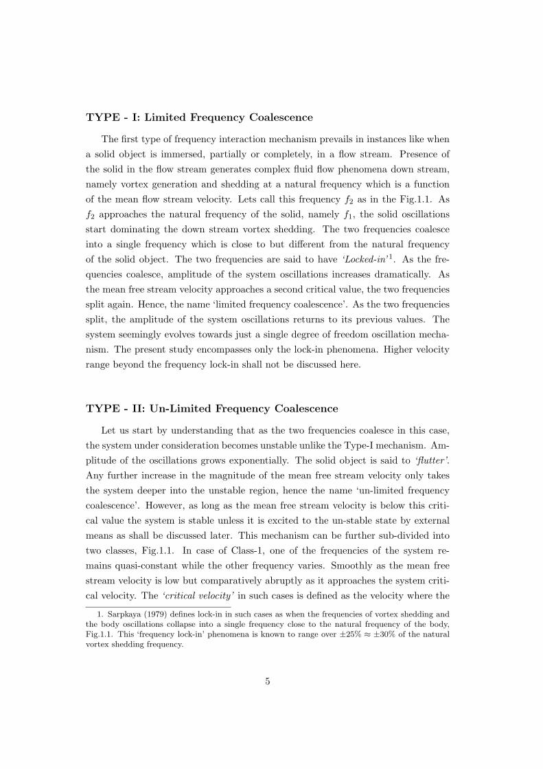
TYPE - I: Limited Frequency Coalescence

The first type of frequency interaction mechanism prevails in instances like when

a solid object is immersed, partially or completely, in a flow stream. Presence of

the solid in the flow stream generates complex fluid flow phenomena down stream,

namely vortex generation and shedding at a natural frequency which is a function

of the mean flow stream velocity. Lets call this frequency f2 as in the Fig.1.1. As

f2 approaches the natural frequency of the solid, namely f1, the solid oscillations

start dominating the down stream vortex shedding. The two frequencies coalesce

into a single frequency which is close to but different from the natural frequency

of the solid object. The two frequencies are said to have ‘Locked-in’ 1. As the fre-

quencies coalesce, amplitude of the system oscillations increases dramatically. As

the mean free stream velocity approaches a second critical value, the two frequencies

split again. Hence, the name ‘limited frequency coalescence’. As the two frequencies

split, the amplitude of the system oscillations returns to its previous values. The

system seemingly evolves towards just a single degree of freedom oscillation mecha-

nism. The present study encompasses only the lock-in phenomena. Higher velocity

range beyond the frequency lock-in shall not be discussed here.

TYPE - II: Un-Limited Frequency Coalescence

Let us start by understanding that as the two frequencies coalesce in this case,

the system under consideration becomes unstable unlike the Type-I mechanism. Am-

plitude of the oscillations grows exponentially. The solid object is said to ‘flutter’.

Any further increase in the magnitude of the mean free stream velocity only takes

the system deeper into the unstable region, hence the name ‘un-limited frequency

coalescence’. However, as long as the mean free stream velocity is below this criti-

cal value the system is stable unless it is excited to the un-stable state by external

means as shall be discussed later. This mechanism can be further sub-divided into

two classes, Fig.1.1. In case of Class-1, one of the frequencies of the system re-

mains quasi-constant while the other frequency varies. Smoothly as the mean free

stream velocity is low but comparatively abruptly as it approaches the system criti-

cal velocity. The ‘critical velocity’ in such cases is defined as the velocity where the

1. Sarpkaya (1979) defines lock-in in such cases as when the frequencies of vortex shedding andthe body oscillations collapse into a single frequency close to the natural frequency of the body,Fig.1.1. This ‘frequency lock-in’ phenomena is known to range over ±25% ≈ ±30% of the naturalvortex shedding frequency.

5

frequencies coalesce. In Class-2 however, ideally both the frequencies mirror each

other’s behavior, Fig.1.1(c). This clear distinction in behavior within Type-II can be

attributed to the existence of strong structural coupling between the two degrees of

freedom in Class-2. In case of Class-1 usually in real life scenarios, structural coupling

between the two degrees of freedom is avoided by manipulating various structural

parameters. It can not however be eliminated entirely given the aerodynamic effects

which reveal themselves in detailed theoretical modelling of such problems. All the

pertinent structural parameters and the added aerodynamic terms shall be identified

and discussed in the following chapters.

In man made systems, Type-I limited frequency coalescence mechanism prevails

largely in human inventions like sky-scrapers, chimney stacks and riser tubes etc.

The Type-II, Class-1 un-limited frequency coalescence mechanism exists more often

in civil constructions like bridge decks. Aircraft structures generally exhibit the

Type-II, Class-2 mechanism. We shall investigate all these cases in more detail

in the chapters which follow. Figs.1.1(a, b & c) correspond to Figs.1.2(a, b & c)

respectively.

6

(a).

(b).

(c).

Figure 1.2: Fluid Structure Interaction Systems. (a). Flow Past a Bluff Body (b).Suspension Bridge at Porte de Millau France (c). Airbus A380 landing at SydneyAirport November 2006.

7

1.2 Limited Frequency Coalescence

Vortex-induced vibration of structures is of practical interest in many fields of

engineering. It can cause vibrations in heat exchanger tube bundles, it influences the

dynamics of riser tubes bringing oil from the sea bed to the surface, it is important

for the design of civil structures such as chimney stacks as well as for the design

of marine and land vehicles. It can also cause large amplitude motions of tethered

structures in the ocean. These examples are just a few from the large spectrum of

problems where vortex-induced-vibrations (VIV) are important.

Vibrations induced by vortices shedding down-stream of a bluff body submerged

in an incident flow have been a subject of vast scientific investigations for a long

time now, Fig.1.3. Wilkinson (1974), Otsuki et al. (1974) and Mizota & Nakamura

(1975) presented some experimental data on the forced oscillations of square section

cylinders. Sarpkaya (1979) presented a selective review of the then existing knowl-

edge bank about vortex induced oscillations. Sarpkaya and the references there in

remark that in case of circular cylinders inclination angle of the cylinder with respect

to the mean free stream apparently does not affect the vortex induced oscillations.

Bearman & Obasaju (1982) conducted a study to compare experimental results for

fixed and forcibly oscillating square cylinders. They determined that the amplifica-

tion of the fluctuating lift coefficient for a square cylinder at lock-in was much less

than that of a circular cylinder subjected to similar conditions. Moreover, at low

reduced velocities phase of the vortex shedding may actually damp out oscillations

of a flexibly mounted cylinder. Below the lock-in range forced oscillations dominate

the system, forcing the vortices to shed at approximately the cylinder frequency. Its

only in the lock-in range that the cylinder executes vortex induced oscillations. Bear-

man (1984) reviewed the vortex shedding phenomena from oscillating bluff bodies.

Ongoren & Rockwell (1988a) studied cylinders of various cross sections executing

forced oscillations while submerged vertically in a water channel. Two different

mechanisms of frequency synchronization based on whether the excitation is sub-

harmonic or harmonic relative to the vortex formation frequency, were outlined. In

a subsequent paper in the same year, they studied the effects of cylinder inclination

with respect to the mean free stream, using a forced circular cylinder in a water

channel. The authors contend that outside the synchronization range the symmetri-

cal and anti-symmetrical modes compete to lock on to the near wake structure. The

number of occurrences of each mode is a function of the excitation frequency and

the inclination angle, Ongoren & Rockwell (1988b). Williamson & Roshko (1988)

8

provided the mechanism of vortex formation and the underlying physics for mode

shifts. The authors concluded that the sudden phase shifts of the lift force with

respect to the body motion can be attributed to the vortex pairing each half cycle

occurring downstream of the bluff body. Parkinson (1989) resumed the phenomenol-

ogy and the theoretical modeling tools available to understand the vortex induced

oscillations and the galloping instability in case of flow past bluff bodies. Brika &

Laneville (1993) studied a hollow slender cylinder in a wind tunnel and showed that

the cylinder’s steady response was hysteretic. Each branch in the hysteresis loop is

associated to either the 2S or the 2P mode of vortex shedding. Abrupt change in

the amplitude curve is attributed to the sudden mode shift. Khalak & Williamson

(1999) conducted an experiment using low mass and low damping. They studied

the effects of varying non-dimensional mass and non-dimensional damping. Govard-

han & Williamson (2000) presented the transverse vortex induced oscillations of an

elastically mounted rigid cylinder in a fluid flow. The authors point out that in a

classical high mass ratio system the initial and lower amplitude branches can be dis-

tinctly identified due to a discontinuous mode transition. In case of lower mass ratio

systems a further upper amplitude branch is clearly identifiable attributed to a sec-

ond instance of mode transition. Extensive details about the vortex shedding mode

formation and the transition from 2S to 2P can be found in Govardhan & Williamson

(2000). Hemon et al. (2006) submitted experimental and numerical results on the

aeroelastic behavior of slender rectangular and square cylinders subjected to a cross

flow. Their study primarily focused on a flexible rectangular cylinder. They noted

that a small increase in the free stream turbulence intensity actually reduces the

critical galloping velocity. Cheng et al. (2003) have discussed the use of piezoelectric

ceramic actuators installed on the bluff body surface. The actuators when operated

would deform the cylinder surface thus modifying the fluid flow and structural vibra-

tion. Facchinetti et al. (2004) have investigated the coupled dynamic behavior of a

circular cylinder using the classical wake oscillator model based on the one proposed

by Currie & Hartlen (1970). The authors have demonstrated that the acceleration

coupling in the forcing term of the wake oscillator best matches with the available

experimental data. Morse & Williamson (2009) discovered the 2Poverlap mode using

high resolution data from a forced oscillating cylinder at a fixed Reynold’s number.

They found that even when the cylinder oscillates with a constant amplitude and

frequency, the cylinder wake can still shift from the 2P to 2Poverlap mode. Also, a

cylinder subjected to a flow could keep on oscillating even if the vortex generation

9

frequency de-synchronizes with the cylinder oscillating frequency. This can be ex-

plained by the presence of a component of fluid forcing at the cylinder oscillation

frequency which yields positive fluid excitation.

Common practice in studying VIV on cables and on slender structures consists in

performing free motion tests in a wind tunnel on sectional models to define the lock-

in region in terms both of vibration amplitudes and width of the synchronization

range and the energy transferred by the wind in the mechanical system.

10

Figure 1.3: Flow Past a Bluff Body by Da Vinci. (www.cora.nwra.com)

11

1.3 Un-Limited Frequency Coalescence

Civil engineering structures like bridge decks may also execute self-excited oscil-

lations and in turn respond to the aerodynamic forces thus generated. One of the

oldest examples of suspended bridge deck failure due to frequency coalescence is the

Angers Bridge in France, although the exact cause of failure in this case is not aeroe-

lastic in nature. The Brighton Chain Pier Bridge, Fig.1.4 and the original Tacoma

Narrows Bridge, Fig.1.5 are notorious examples of bridge failure due to aeroelastic

effects.

Figure 1.4: Chain Pier Brighton, Artist: Clem Lambert. (en.structurae.net)

Aerodynamic performance of bridges is very sensitive to sectional shape and

detailed structure of the section. Studies aimed at investigating the bridge deck

behavior at lock-in wind speeds have increasingly found space in modern bridge con-

struction projects. Recent developments in the long span suspension bridge deck

design and huge on-going projects across the globe have strengthened the need to

investigate this phenomenon. Storebaelt Suspension Bridge in Denmark is a real life

example where vortex shedding downstream of the deck section caused low frequency

oscillations. Subsequent investigations in a wind tunnel revealed lock-in at existing

12

Figure 1.5: Tacoma Narrows moments before the collapse.

wind speed conditions, Larsen et al. (2000).

Scanlan & Tomko (1977) showed conclusively that though helpful, the Standard

Airfoil Theory has very distinct limitations in case of bridge deck sections. Aerody-

namic flutter derivatives calculated even for stream-lined bridge deck sections showed

limited resemblance with those of a symmetric airfoil. The most important difference

as pointed out in Scanlan & Tomko (1977) is the difference between the added aero-

dynamic damping coefficient for an airfoil and for a bridge deck. Some streamlined

bridge decks may exhibit similar coefficients as those of an airfoil, attention must be

paid that any such resemblance is necessarily limited. Nakamura (1978) submitted

a set of analytical formulas applied to the bi-modal bridge deck flutter. Larose &

Mann (1998) presented an analytical model independent of the strip assumption to

predict the gust loading effects on a streamlined bridge deck subjected to isotropic

turbulence. The strip assumption is known to be a source of error in the analytical

prediction methods used to predict the aerodynamic behavior of closed box girder

bridge decks. Chen et al. (2000) investigated the effect of aerodynamic coupling be-

tween the modes on the flutter and buffeting response of a bridge deck. They solved

the equations of motion of an aeroelastic bridge deck section using complex eigen

13

value analysis to study the self-excited forces and their effects on modal frequencies,

inter-modal coupling and damping ratios as functions of wind velocity. The authors

concluded that the symmetric vertical and torsional modes are the dominant modes

for coupled flutter. The coupled self excited forces acting on the bridge deck are

primarily responsible for the negative damping which in turn causes flutter. These

coupling effects may cause flutter at lower velocities as predicted by the conventional

mode by mode approach in case of relatively bluff bridge deck sections. Chen et al.

(2002) proposed a method exploiting the general least square theory for identifying

the flutter derivatives of a three degree of freedom bridge deck section. Banerjee

(2003) submitted an analytical method for the free vibrations and flutter analysis

of bridge decks using the normal modes method and generalized coordinates. Chen

(2007) proposed a new frame work for estimating the modal frequencies, damping

ratios and coupled oscillations of a two degree of freedom aeroelastic bridge deck

system subjected to varying wind velocities. Matsumoto et al. (2007) resumed the

evolution of our know-how about the flutter instability in bridge decks. The authors

pointed out the most effective flutter derivatives which can be exploited to counter

the flutter instability in such cases. Detailed discussion on flutter derivatives shall

follow in Sec.3.1. Bartoli & Mannini (2008) showed that the contribution of struc-

tural damping in on-setting flutter cannot always be neglected depending on the

dynamic and aerodynamic properties of the bridge deck. Neglecting the structural

damping may result in an in-accurate prediction of the critical fultter velocity.

The present study explores the long term and transient stability phenomena in

case of bridge deck sections. Most bridge deck sections, except very stream-lined,

behave like bluff bodies and the airflow is essentially separated down-streams. Cross

section aerodynamics of the bridge deck is often optimized by modifying shape and

non-structural parameters. Sometimes dynamic parameters like the frequency ratio

are also adjusted to increase the flutter critical wind speed. Prediction of the critical

flutter speed remains one of the most important design procedures for modern long

span suspension bridges.

Frequency Coalescence in Airfoil Sections

Aircraft wings and control surfaces have been known to oscillate since early days.

Consider a simple rigid airfoil without sweep in a wind tunnel with a small angle of

attack. In the absence of any flow, any forced vibration would damp out gradually.

14

As the flow speed in the wind tunnel increases, the rate of damping first increases.

With further increase in the flow velocity, a point is reached at which the damping

decreases rapidly. At the critical flutter speed an oscillation can just maintain itself

with steady amplitude. At flow velocities beyond this critical value, a small acci-

dental disturbance of the airfoil can serve as a trigger to initiate oscillations with

an increasing amplitude. In such circumstances the airfoil suffers from oscillatory

instability and is said to ‘flutter’.

The first recorded flutter victim was a Handley Page O/400 twin engine bi-plane

bomber in 1916. Bairstow & Fage authored the first theoretical flutter analysis in

1916, Fig.1.6. They investigated binary flutter; twisting of the fuselage and motion

of the elevators about their hinges, Garrick & Wilmer (1981). H. Reissner in 1926;

developed a detailed analysis of wing torsional divergence, showing the importance

of relative locations of the aerodynamic center of pressure and of the elastic axis,

Garrick & Wilmer (1981).

Von Schlippe formulated the first ever flutter test in 1935 in Germany, Kehoe

(1995). He plotted the amplitude of an airframe forced to oscillate at resonating fre-

quencies as a function of airspeed. Increase in amplitude suggested reduced damping.

Flutter was thought to occur at the asymptote of theoretically infinite amplitude as

shown in Fig.1.7.

Theodorsen & Garrick (1940) compiled the results of the then existing basic flut-

ter theory and the large number of experiments that were being conducted at that

time. Kholodar et al. (2004) studied the effects of structural parameters and free

stream Mach number on the Limit Cycle Oscillation (LCO) characteristics of a typ-

ical two degrees of freedom transonic airfoil configuration. They concluded that the

stability of the limit cycle oscillations is very sensitive to the changes in the Mach

number in the transonic range. Lee et al. (2005) studied a two degrees of freedom

airfoil in sub-sonic flow with cubic non-linear stiffnesses at the supports. Exploiting

the Quasi-Steady Aerodynamic Theory they formulated three fast frequency com-

ponents to study the dynamics of fluid structure interaction. Their study showed

that an initial excitation of the bending mode triggers the excitation of the torsional

mode through non-linear interaction. Hemon et al. (2006) presented an extensive

experimental study of coupled mode airfoil flutter with reference to the transient

15

Figure 1.6: Historic Tail Plane Flutter Analysis given by Bairstow & Fage in 1916,Garrick & Wilmer (1981). Modern theoretical tools used to study flutter are basedon Theodorsen’s General Theory of Aerodynamic Instability. Theodorsen’s methodto solve the equation for flutter stability differs from his predecessors. This dif-ference exists because he deals with pure sinusoidal motion applied to a case ofun-stable equilibrium. He therefore, does not make use of the Routh’s discriminant,Theodorsen (1935) .

growth of energy in the system. Experimental data showed that the maximum en-

ergy amplification attained in such a system does indeed vary with the magnitude of

the imposed initial conditions. In these experiments however, upstream turbulence

was very low. The airfoil was excited by physical mechanical means like dropping

a fixed weight from a controlled height. Experimental results were later compared

with the simulations using the Unsteady Airfoil Theory and were found to be in

good agreement. Shams et al. (2008) presented a method for non-linear aeroelastic

analysis of a slender airfoil. They showed that the Unsteady Linear Airfoil Theory

based on the Wagner function agreed well with the results obtained from their test

case. Limitations of the theory in predicting the physical phenomenon beyond the

critical flutter limit was pointed out.

16

Figure 1.7: Von Schlippe’s Historical Flight Flutter Test Method, Kehoe (1995).

Presenting a comprehensive chronological overview of the discoveries in this field

is not the aim here. It would suffice to say that flutter has remained a subject

of intense research ever since. Despite the tremendous advancement in our under-

standing of the flutter phenomena and the development of the state of the art flutter

testing techniques, it keeps occurring. Recent examples of flutter related incidents

in the aviation industry include Taiwan’s IDF fighter, which crashed due to flutter

of horizontal tail during high dynamic-pressure flight-test in 1992. Later in the same

year, a prototype of the U.S. F-22 crashed in a flutter related accident. In September

1997, a U.S. Air Force F-117 crashed due to flutter excited by the vibration from

a loose elevon. Every year many small airplanes, usually the home-built, continue

to become casualties of flutter. Boeing started flutter testing of its 787 Dream liner

in February 2010. As obvious, flutter still attracts tremendous potential for further

research. It continues to remain a hugely important aspect of modern aircraft design.

In this work we shall investigate the by-pass tansition to flutter due to transient

growth of energy in case of an airfoil with coupled two degrees of freedom. We

shall demonstrate how the simple quasi-steady theory coupled with the Kussners

aerodynamic admittance function can qualitatively predict the airfoil behavior. The

airfoil experimental set-up is similar to the one described in Schwartz et al. (2009).

Scope of this work is limited to two dimensional incompressible flow past a symmetric

airfoil.

17

1.4 Problematic

Fluid structure interaction systems as outlined in the previous sections encom-

pass a broad horizon of our daily lives. Given the natural tendency of things to move

towards chaos, all efforts are spent to find out and understand any possible mecha-

nisms which could lead a fluid structure system inch towards an un-stable state. As

the title of the thesis suggests; purpose of this study is to investigate various fluid

structure interaction systems with focus on their behaviors both in the long-term

and short-term. The later is commonly referred to as Transient Behavior. Various

standard measurements like the critical velocities and natural frequency evolution

provide important information regarding the long-term response of a fluid structure

interaction system. Careful caliberation, detection and measurement of these pa-

rameters plays an important role towards reliable scientific investigation. Findings

from these experimental procedures are then put to use to study the more complex

short-term or transient dynamic properties of the system which are inherently elusive

and complicated to reproduce in a lab environment. For example, critical velocity

measured is commonly used to normalize the mean free stream velocity while study-

ing the transient behavior of such systems close to their linear stability limits.

Traditionally, investigations of the stability properties of a flow were treated as

eigen value problems. It was established that exponentially growing eigen modes in

a system cause the instability. In some cases however, a system may transition to

an unstable state even in the absence of primary exponential instabilities as men-

tioned above. This type of instability mechanism is known as the ‘by-pass transition’.

Given all the above, it is needless to point out that although proven experimental

techniques exist to study the long-term behavior of various systems, its awareness

and anticipation of various crucial system parameters remains of profound practical

importance. At the same time, as we shall see during the course of this study, tran-

sient behavior of a system has proven to be critical in understanding various new

failure mechanisms as discovered in the field of fluid structure interaction and briefly

summarized in the preceeding sections.

Recently, a number of theoretical and numerical studies have explored the pos-

sibility of exsitance of transient instability mechanism in case of fluid structure in-

teraction systems. Schmid & de Langre (2003) applied the concept of transient

growth of energy to coupled mode flutter, Type-II fluid structure system, Fig.1.1.

The authors found that energy of a coupled two degree of freedom system can be

18

amplified by a factor of 10 by the transient growth. The magnitude of this tran-

sient amplification is large enough to qualify as a discrepancy from the threshold

predicted by the linear stability theory. Noger & Hemon (2004) presented a study

showing the existence of transient amplification of energy in case of automobiles.

Hemon et al. (2006) presented experimental evidence of transient amplification of

energy before airfoil flutter. The authors established that natural transient loading

may trigger large amplitude oscillations at linear sub-critical flow velocities; in such

systems. Needless to mention here that transient amplification of energy in fluid

structure interaction systems has attracted some attention only recently. Very little

experimental data exists, Hemon et al. (2006), to verify the theoretical predictions.

More detailed experimental investigations are needed.

The present study is an experimental investigation of the long-term and transient

behavior of fluid structure systems with two degrees of freedom. We shall present

our findings based on three case studies under taken during the course of this work.

Each case study is based on a bluff body subjected to a uniform incident flow. This

report is divided into two parts based on the long-term and transient properties of

the experimental setups. We shall discuss the long term behavior of a bluff body

system executing vortex induced vibrations in the first part. Moreover, long term

stability parameters for an airfoil and a bridge deck system are also included. The

second part is dedicated to the transient behavior of all the three fluid structure

systems. We have organized the fluid structure interaction systems into two types

based on how the natural frequencies of the system behave as linear stability thresh-

old is approached, Section1.1, Fig1.1.

We shall start our inquisition firstly by a Type-I system, Fig.1.1. The most sim-

ple Type-I fluid structure system is depicted by the classical flow past a bluff body

setup. One of the most intriguing phenomenas related to the investigations of flow

past a freely oscillating bluff body is the existence of hysteresis in the amplitude vari-

ation and the frequency capture depending on the approach to the resonance range -

from lower velocities or from higher velocities. As cataloged in the previous sections,

it appears that very few experimental studies have focused on the existence of hys-

teresis in case of freely oscillating square cylinders. Some data obtained from freely

oscillating circular cylinders can be obtained from Feng (1968) and Brika & Laneville

(1993). Cheng et al. (2003) have presented some data on a freely oscillating square

cylinder. None of these works presents data concerning transient regime. The vortex

19

shedding oscillations of high mass ratio structure is therefore not well documented

for a freely oscillating square section despite its obvious interest in civil engineering

problems. In the present study we shall present results obtained from a freely oscil-

lating square cylinder in a vertical wind tunnel. Reduced amplitude curves of the

oscillating cylinder obtained under different experimental configurations provide in-

sight to the long term behavior of such systems. Experimental data is compared with

the results obtained by numerically simulating a theoretical wake-oscillator model.

Wind tunnel measurements of the reduced growth rate in the transient regime are

discussed in Part-II of the study. The experimental findings were used to validate a

wake oscillator model presented by Facchinetti et al. (2004).

Type-II fluid structure interaction systems are studied for two cases. Firstly, the

aeroelastic behavior of a linear two degrees of freedom bridge deck is studied in a

horizontal wind tunnel. Most bridge deck sections are not streamlined so that flow

around the cross section is necessarily separated. On the other hand most bridge

deck sections are not very bluff so there may be a net lift/drag force acting on the

deck section. In the present study, flow around the bridge deck section generates

a net lift force pushing the bridge deck downwards in the wind tunnel test section.

This new position is taken as reference for subsequent energy calculations. Extensive

experimental evidence is provided to study the effects of frequency ratio on the evo-

lution of maximum normalized energy of the system and the critical flutter speed.

We shall define our frequency ratio and see how the maximum energy amplification

of a bridge deck section can be controlled by manipulating the frequency ratio pa-

rameter. Accurate experimental evidence is also provided linking the critical flutter

velocity and the frequency ratio of the system. The present work is limited to lower

Reynolds Number and the turbulence level upstream of the test section is kept very

low. We have studied a stream-lined bridge deck profile resembling that of the cable-

stayed road bridge constructed over the valley of river Tarn near Millau in Southern

France, Fig.1.2(b).

Secondly, another important fluid structure interaction system which exhibits

Type-II frequency coalescence mechanism, Fig.1.1, but which is fundamentally dif-

ferent from the bridge deck is the airfoil system. As pointed out earlier with reference

to Scanlan & Tomko (1977) Standard Airfoil Theory has distinct limitations when

applied to bridge deck sections. End plates are used to ensure two dimensionality of

the setup. This experiment builds onwards from the experimental study presented

20

in Hemon et al. (2006). We added an aluminum flap to the system to create an

up-stream gust. The gust is allowed to excite the airfoil in the test section. This

brings the experimental set-up closer to the real world scenario where aircrafts are

often subjected to gusts in flight. Results obtained by this experimental procedure

are compared with the already existing classical airfoil theories. The experiment is

repeated for another airfoil setup with weak non-linearity in the system stiffness.

Results obtained by both linear and non-linear experimental setups are compared to

establish the existence of by-pass transition to flutter, Sec.6.3. Furthermore, a new

cobmination of the standard quasi-steady theory and the Kussners aerodynamic ad-

mittance function is proposed to validate the transient energy amplification results

obtained for the linear airfoil setup. Airflow over the profile has been treated as in-

compressible in the simulations. All the experimental results and our findings from

the comparison shall be discussed in subsequent chapters.

In the end, our findings from the study, some suggestions regarding the possi-

bilities for further investigations and a bibliography of the literature consulted shall

conclude this study.

21

PART-I Long Term Behavior

Part-I of this thesis report is dedicated to the long-term behavior of different

fluid structure interaction systems, Sec.1.4. As pointed out earlier, various standard

measurements including the critical velocities and frequency evolution provide im-

portant information regarding the long term response. Accurate knowledge of these

parameters is important because the results obtained in this part shall be used in the

more complex transient study in Part-II. For example, awareness of the frequency

evolution in the presence of dynamic wind conditions enables us to determine how

the energy amplification due to transient growth is linked to the frequency ratio in

case of bridge deck sections, Chapter 5.

We shall start with the long-term limit cycle behavior of a square cylinder os-

cillating freely in a high mass ratio environment. The present study differs from

its predecessors in the sense that while the flow velocity and elastic system param-

eters are closely controlled, the square cylinder is allowed to oscillate freely under

the effect of incident air flow. The existence of hysteresis in the reduced amplitude

result is demonstrated using credible experimental data. Experimental results are

compared with the findings from a wake-oscillator model. Discrepencies in the lo-

cation of maximum amplitude and the frequency lock-in range are pointed out and

discussed. Next, we move on to a similar long-term analysis of an airfoil and a bridge

deck system. We submit our experimental setups with low structural damping and

inherently protected from friction losses. An Aluminum flap is used to generate a

single gust. All the measured system parameters are verified using results from nu-

merical simulations. Our experimental findings are presented and discussed in terms

of critical velocities, frequencies and dampings.

Chapter 2

Behavior of a Square Cylinder in

a Wind Tunnel at Low Velocity

In this chapter we shall present experimental results obtained in a wind tunnel

for an elastically mounted rigid square cylinder restrained to move in the transverse-

wind direction. Structural supports of the set-up are assumed to behave linearly

through out the amplitude envelope. Measurements consist of the time histories

of oscillations using laser displacement sensors. All the structural parameters are

estimated without airflow. The behavior of the vortex-induced oscillation is studied

using two configurations. In the first case, the cylinder was brought to rest and

then allowed to oscillate freely for each increment in velocity. In the second case

however, the cylinder was not brought to rest for any velocity increment so as to

study the memory effects on the cylinder amplitude. The classical mode switch can

be observed in both the cases. Hysteresis is however found only in the later case.

Results for both the cases are presented and discussed.

We know that, a bluff body when placed in a fluid stream; generates separated

flow. In the creeping steady flow regime where Re < 1, viscous diffusion dominates

most of the flow and Stokes solution applies to the system. A symmetrical un-

separated flow surrounds the body. No significant changes take place until Re > 5.

The flow remains stable but a re-circulation bubble appears behind the body. As

the Re > 48.5, a typical Benard-Karman vortex street appears behind the bluff

body, Godreche (1998). This vortex shedding and general wake turbulence induce

fluctuating pressure on the body surface, in a direction away from the last detached

vortex, which can in turn cause the body to oscillate. The body is set to oscillate

26

in a direction normal to the mean flow. Amplitude of the oscillation can vary from

1.5 to 2 body diameters. For large amplitude oscillations of a body in high mass

ratio configuration, frequency of body oscillations is close to its natural frequency,

Bearman (1984).

2.1 Experimental Methods

2.1.1 Experimental Set-up

The square cylinder has a cross section, D = 0.02 m and a span, b = 0.15 m.

The cylinder is put in place in the test section using four linear springs mounted

outside the test section. Specific chord wiring is used to restrain the cylinder such

that it oscillates transverse to the air flow. Special attention is paid to keep the

structural damping as low as possible. The experiment is conducted in a vertical

axis Eiffel Wind Tunnel which has a closed circular test section of diameter 0.20

m. A centrifugal fan, down stream of the test section is used to produce the wind

stream. This free stream flow velocity can be safely assumed to be uniform over the

cylinder span given the comparison between the cylinder span and the test section

diameter. Mean velocity in the test section varies from ≈ 2 m/sec to ≈ 7 m/sec for

this experiment. Turbulence level of the upstream airflow is less than 1% over the

velocity range during the course of this study, Amandolese & Hemon (2010), Fig.2.1.

No endplates have been used in the experiments. Due to the aspect ratio of the

cylinder (b/D = 7.5), flow around the longitudinal ends can have a significant effect

on the vortex dynamics, the correlation of the induced fluid forces on the body and

thus the vibrations. Meanwhile the proximity of both the ends of the cylinder with

the test section wall could reduce the effect of the end conditions. As reported by

Morse et al. (2008), for a circular cylinder the vortex-induced vibrations for attached

and un-attached endplates are nearly the same.

2.1.2 Measurement System

Accurate measurement of low velocities is always difficult to achieve. In the

present case, a nozzle is mounted down-stream of the test section. Bernoulli’s The-

orem is used to calculate the air flow velocity in the test section compared with the

flow velocity in the nozzle section. Pressure readings in the test section and the

nozzle section are obtained by using pairs of static pressure taps in each section. A

27

Figure 2.1: Sketch showing the principles of the experimental setup Amandolese &Hemon (2010).

thermocouple is used to implement temperature correction. This technique allows us

to measure low flow velocities with accuracy better than 1%, Amandolese & Hemon

(2010).

Measurements of the transverse displacement of the cylinder are obtained by a

laser displacement sensor. The measurement resolution is 40µm and the accuracy

is 1% of the full scale range. Signals from the laser displacement sensors are trans-

mitted to an acquisition system named PAK provided by Mueller-BBM. It consists

mainly of a 24-bit and 8-channel acquisition card and a signal processing software.

Sampling resolution is 1024 Hz and the typical duration of data accumulation is 60

s. This duration was increased to 300 s for the frequency measurements of the LCO

of the cylinder. Increasing the duration enabled us to obtain a better frequency

resolution for the measurements. The physical degree of freedom z is provided by

the recombination of the measured signals using the system kinematics, Amandolese

& Hemon (2010).

28

Strouhal number of the cylinder was measured while at rest using the spectral

analysis of the unsteady wake. Measurements were obtained by a single component

hot wire anemometer installed down-stream of the square cylinder at a distance equal

to one length of the cylinder side. The Strouhal number was found to be 0.127 over

the velocity range of the vortex shedding oscillation regime, Amandolese & Hemon

(2010).

2.1.3 Identification of Structural Parameters

We have a rigid square cylinder of side ‘D’. The cylinder is constrained to oscil-

late in a direction normal to the mean flow direction as depicted in Fig.2.2.

Figure 2.2: Schematic for Square Cylinder Coupled Wake Oscillator for 2D VortexInduced Vibrations in a Vertical Wind Tunnel.

Flow is assumed to be uniform all along the cylinder length. The cross flow

displacement ‘z’ of the cylinder can be described by the standard damped linear

oscillator as in Eqn.2.1.

mz + rz + kz = S (2.1)

29

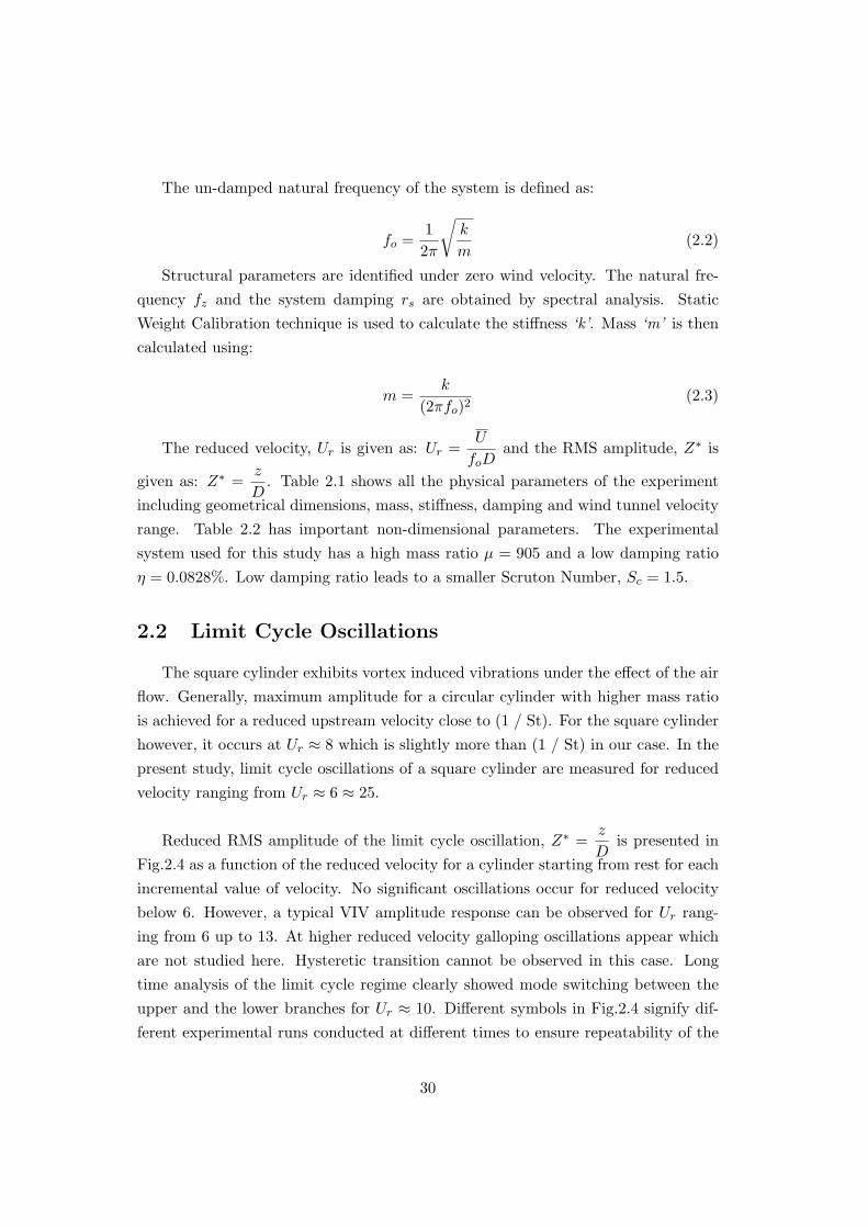
The un-damped natural frequency of the system is defined as:

fo =1

2π

√

k

m(2.2)

Structural parameters are identified under zero wind velocity. The natural fre-

quency fz and the system damping rs are obtained by spectral analysis. Static

Weight Calibration technique is used to calculate the stiffness ‘k’. Mass ‘m’ is then

calculated using:

m =k

(2πfo)2(2.3)

The reduced velocity, Ur is given as: Ur =U

foDand the RMS amplitude, Z∗ is

given as: Z∗ =z

D. Table 2.1 shows all the physical parameters of the experiment

including geometrical dimensions, mass, stiffness, damping and wind tunnel velocity

range. Table 2.2 has important non-dimensional parameters. The experimental

system used for this study has a high mass ratio µ = 905 and a low damping ratio

η = 0.0828%. Low damping ratio leads to a smaller Scruton Number, Sc = 1.5.

2.2 Limit Cycle Oscillations

The square cylinder exhibits vortex induced vibrations under the effect of the air

flow. Generally, maximum amplitude for a circular cylinder with higher mass ratio

is achieved for a reduced upstream velocity close to (1 / St). For the square cylinder

however, it occurs at Ur ≈ 8 which is slightly more than (1 / St) in our case. In the

present study, limit cycle oscillations of a square cylinder are measured for reduced

velocity ranging from Ur ≈ 6 ≈ 25.

Reduced RMS amplitude of the limit cycle oscillation, Z∗ =z

Dis presented in

Fig.2.4 as a function of the reduced velocity for a cylinder starting from rest for each

incremental value of velocity. No significant oscillations occur for reduced velocity

below 6. However, a typical VIV amplitude response can be observed for Ur rang-

ing from 6 up to 13. At higher reduced velocity galloping oscillations appear which

are not studied here. Hysteretic transition cannot be observed in this case. Long

time analysis of the limit cycle regime clearly showed mode switching between the

upper and the lower branches for Ur ≈ 10. Different symbols in Fig.2.4 signify dif-

ferent experimental runs conducted at different times to ensure repeatability of the

30

Figure 2.3: Time evolution of the cylinder motion amplitude at U=2.5155 m/s Aman-dolese & Hemon (2010).

experimental procedure. Apart from the obvious dispersion of experimental points

at higher reduced velocities we can safely assume that the resonant frequencies lie

approximately in the same reduced velocity range for each experimental run.

In the VIV regime the amplitude data shown in Fig.2.4 are very similar to those

carried out by Feng (1968) for a circular cylinder in airflow. Results obtained by

Feng (1968) show two amplitude branches, which were later named as the ‘initial’

and the ‘lower’ branch in Khalak & Williamson (1999). The maximum oscillation

amplitude occurs on the initial branch for a reduced velocity close to 10 which is

significantly above the pure resonant point expected for a reduced frequency close

to 8 (≈ 1/St). This off-set of the maximum value of amplitude from the expected

value of reduced velocity, Ur can be attributed to the blockage effects in the wind

tunnel test section.

A second series of experiments was conducted where the cylinder was not brought

to rest so as to study the memory effects on the cylinder amplitude. Results are re-

ported in Fig.2.5, where circular points represent experimental data recorded while

increasing the velocity by a fixed increment and cross points represent data accumu-

lated while decreasing the free stream velocity using a fixed decrement. As was the

31

6 8 10 12 14 16 180

0.02

0.04

0.06

0.08

0.1

0.12

0.14

0.16

0.18

0.2

Ur

Z∗

Figure 2.4: Reduced RMS Amplitude of the limit cycle oscillations versus reducedvelocity; without Memory Effect.

case in Fig.2.4, reduced RMS amplitude of the limit cycle oscillation is presented as

a function of the reduced velocity. We see that in this case also, the typical VIV

response is observed for the same reduced velocity range, from 6 to 13.

Results, obtained from the experiments which allowed the memory effect, exhibit

an upper and a lower branch with an abrupt transition for a reduced velocity ≈ 9.5.

Williamson & Roshko (1988) used visualisations attributing the sudden change in

magnitude to an abrupt mode switch which in turn can be explained by the abrupt

shift in phase angle between the vortex shedding frequency and the cylinder oscil-

lating frequency. They showed that the fluid stream just below the critical reduced

velocity is extremely sensitive and a very small disturbance is enough for the system

to go from one equilibrium state to another thereby causing an abrupt change in

formation named as ‘the mode-jump’. Brika & Laneville (1993) found that these

amplitude branches correspond to different synchronized vortex wake patterns. The

‘upper’ branch in the amplitude response lies in the von Karman type 2S mode of

the Williamson-Roshko map of wake patterns. The ‘lower’ branch however lies in

the 2P mode regime in which two vortices of opposite sign are shed from each side of

the cylinder at every oscillation cycle. The probability of the existence of 2S mode

32

6 7 8 9 10 11 120

0.02

0.04

0.06

0.08

0.1

0.12

0.14

Ur

Z∗

Figure 2.5: Reduced RMS Amplitude of the limit cycle oscillations versus reducedvelocity; (o) increasing velocity, (x) decreasing velocity.

decreases as Ur is increased. A slight hysteretic effect can be observed for Ur ≈ 9.5.

Following the circular points as the reduced velocity is increased by a fixed incre-

ment, a relatively smooth mode switch to the lower branch can be noticed for a

reduced velocity slightly above 9.5. Following the cross points while decreasing the

free stream velocity using a fixed decrement, an abrupt mode switch takes place at

reduced velocity slightly lower than 9.5. We can observe that the RMS amplitude

routes for the square cylinder tend to superimpose except for a very brief interval

of reduced velocity in the vicinity of the mode switch. The maximum oscillation

amplitude found in this case is clearly less than 0.20D. This maximum amplitude is

smaller than the maximum amplitude predicted for a circular cylinder in air flow by

Brika & Laneville (1993) and later catalogued by Khalak & Williamson (1999). The

amplitude levels presented in Fig.2.5 are also significantly lower than for the starting

from rest configuration.

It is important to note here that the maximum amplitude location in both the

cases is off-set from its expected value of (1 / St). This off-set may be attributed to

the blockage effect in the test section. However, the fact that in case of the growth

rate measurements of the same cylinder the maximum growth rate value lies very

33

close to (1 / St) adds to the complexity of apparently a simple phenomenon. We

shall discuss the growth rate measurements in more detail in Sec.4.2.

2.3 Comparison with Theoretical Model

2.3.1 Theoretical Model

For a one dimensional case the equation of motion of a rigid cylinder oscillating

in the transverse z-direction (normal to the flow) reads as Eqn.2.1, where, ‘m’ is the

mass of the cylinder, ‘r’ is a viscous damping coefficient, ‘k’ is the stiffness of the

setup and ‘S’ is the aerodynamic force resulting from the fluid structure interaction

in this case, mainly due to vortex shedding.

The mass ‘m’ takes into account the cylinder mass and the fluid added mass mf

which models the inviscid inertial effects. Following Blevins (1990) we can precise:

m = ms + mf ; mf = CMaρD2 π

4; µ =

m

ρD2(2.4)

where, ‘ρ’ is the fluid density (in our case air), ‘µ’ is a dimensionless mass ratio

and ‘CMa’ is the added mass coefficient. Similarly, following Blevins (1990) we can

write the system damping:

r = rs + rf ; rf = γΩρD2 (2.5)

where ‘γ’ is a stall parameter as Skop & Balasubramanian (1997) and ‘Ω’ is a

reference angular frequency. Assuming that the mean free stream velocity ‘U’ is zero,

‘Ω’ is the angular frequency of the structure oscillation and ‘γ’ is a function of the

amplitude of oscillations related to the mean structural drag coefficient CD, Blevins

(1990). Blevins (1990) defines ‘γ’ for a circular cylinder as:

γ =1

4πStCD (2.6)

In our case however, ‘Ω’ is the vortex shedding angular frequency, Ω = Ωf =

2πStU

D. ‘St’ is the Strouhal Number. Following Skop & Balasubramanian (1997)

‘γ’ shall be assumed to remain constant for the sake of simplicity. Govardhan &

Williamson (2000) used two distinct formulations of the equation of motion for the

‘total force’ and the ‘vortex force’. Following the same approach the fluid effects

namely the added mass and added damping have been included directly in the

34

structural oscillatior in Eqn.2.1 through Eqn.2.4 & Eqn.2.5. The vorticity effects

are modelled by the forcing term at the right hand side in Eqn.2.1. Structural an-

gular frequency Ωs is typically defined as Ωs =

√

k

mand the reduced structural

damping ξ =rs

2mΩs

. Eqn.2.1 can be rewritten as:

z +

(

2ξΩs +γ

µΩf

)

z + Ω2sz =

S

m(2.7)

Standard van der Pol equation is used to model the fluctuating nature of the

vortex street down stream of the oscillating square cylinder.

q +(

ǫΩf

(

q2 − 1))

q + Ω2fq = F (2.8)

The fluid variable ‘q’ is defined as the reduced vortex lift coefficient. Mathemat-

ically, q = 2CL

CLo

. CLo is the reference lift coefficient measured on a fixed cylinder

subjected to vortex shedding. ‘F’ shall be ‘Az’ for displacement coupling, ‘Az’ for

velocity coupling and ‘Az’ for acceleration coupling. Facchinetti et al. (2004) have

presented a detailed study of the dynamics of such a coupled system. They estimated

the near wake van der Pol parameter ‘ǫ’ and the coupling force scaling ‘A’ from the

available experimental data. The oscillation amplitude at lock-in zM is obtained

from:

zM =CLo/2

SG + 4π2St2γ

√

1 +A

ǫ

CLo/4

SG + 4π2St2γ(2.9)

see Facchinetti et al. (2004) for algebraic details.

2.3.2 Den Hartog’s Instability Criteria

It should be kept in mind here that the model proposed by Facchinetti et al.

(2004) as discussed above is valid for circular cylinders. The present study however

is based on the vortex induced vibrations of a square section cylinder. It is imperative

to remark here that this basic difference in geometery has to be taken into account

to be able to compare theoretical findings and experimental results later. Blevins

(1990) suggested a simplified system to be considered, Fig.2.6.

The angle of attack ‘α’ can be calculated as α = tan−1

(

z

U

)

such that if α = 0;

z = 0 implying that the cylinder is at its equilibrium position. Also, if ‘α’ is very

35

FL

FD

Figure 2.6: Single Degree of Freedom Galloping Model. Reproduced as Blevins(1990).

small α ≈ z

Uand Urel ≈ U . Now from the Fig.2.6, the resultant vector is assumed

positve downwards:

Fz = −FLcos (α) − FDsin (α) =1

2ρU2DLCz (2.10)

where Cz is the vertical force coefficient

Cz = −U2rel

U2[CLcos (α) + CDsin (α)] (2.11)

Now because α is very small, advancing Eqn.2.11:

Cz (α) = −CL −(

−∂CL

∂α+ CD

)

α (2.12)

In the last equation if∂Cz

∂α< 0 or equivalently

∂CL

∂α+ CD > 0, total damping of

the system remains positive. The system remains stable. This is known as the Den

Hartog’s Stability Criteria. Equation 2.12 at α ≈ 0 gives Cz = CL. Trivial algebraic

manipulation of Eqn.2.10 and Eqn.2.12 yield:

Fz = −1

2ρU2DLCL +

1

2ρUDL

∂Cz

∂αz (2.13)

36

Comparing Eqn.2.1 and Eqn.2.13, retaining only lower order terms of α, we arrive

at:

γ =1

8πSt

∂Cz

∂α(2.14)

where,∂Cz

∂αis 3 for a square cylinder in smooth flow and 3.5 for a square cylinder

in turbulent flow, Blevins (1990).

Investigations by Facchinetti et al. (2004) revealed that using acceleration cou-

pling in the forcing term of the wake oscillator best matches with the then available

experimental results. The coupling terms were formulated to essentially allow only

the linear functions of the wake variable ‘q’ and displacement ‘z’ and their temporal

derivatives. In order to set the values of parameters ‘A’ and ‘ǫ’, the total lift coeffi-

cient was assumed to be the same as the vortex lift coefficient. Although Facchinetti

et al. (2004) recommend acceleration coupling as the most suitable, it is important

to keep in mind that the theoretical model was devised for systems with lower mass

ratios. Since this experimental work involves higher mass ratio system we refer to the

lock-in domain calculations as a function of mass ratio by the same authors. Given

the seemingly asymptotic relationship between the upper and lower bounds of the

lock-in region in the velocity coupling model at lower mass ratios, we can conclude

that it is the velocity coupling model which is best suitable for our high mass ratio

experimental setup. This study therefore focuses on the velocity coupling model.

Following the same approach as Facchinetti et al. (2004) and the references there

in, we solved the model numerically as presented in Eqn.2.7 and Eqn.2.8 using the

Fox and Goodwin iteration scheme. Details of the iteration scheme shall be described

in Sec.3.1. System parameters are described in Table 2.1 and Table 2.2, Fig.2.7.

37

6 7 8 9 10 11 12 130

0.02

0.04

0.06

0.08

0.1

0.12

0.14

0.16

0.18

Ur

Z∗

6 7 8 9 10 11 12 131.95

2

2.05

2.1

2.15

2.2

2.25

2.3

2.35

2.4

Ur

q

Figure 2.7: Hysteresis Standard Wake-Oscillator Model Solved Numerically usingVelocity Coupling as in Facchinetti et al. (2004). (Solid-Line) Increasing Velocity,(Dashed-Line) Decreasing Velocity. Z* is the amplitude normalized with respect tothe dimension ‘D’ of the Square Cylinder, Fig.2.2.

38

As discussed in Sec.1.1, experimental results presented in Fig.2.4 and Fig.2.5 can

be explained by the Type-II frequency coalescence mechanism, Fig1.1. As obvious

from Fig.1.1, no significant oscillations take place at lower reduced mean free stream

velocities, Ur, when the two natural frequencies of the system are far apart. The

fluid structure interaction mechanism is dominated by the inertial effects due to the

in coming flow. As the Ur increases, the vortex shedding frequency down streams of

the cylinder gets increasingly synchronized with the cylinder oscillating frequency.

This results in an increasing energy transfer from the wake to the oscillating cylinder.

Facchinetti et al. (2004) have stated that for a positive energy transfer of this sort,

0 < −ϕ

π< 1, where ϕ is the phase angle between the vortex shedding frequency and

the cylinder oscillating frequency. Increased energy transfer shows as higher cylinder

oscillating amplitude. The cylinder exhibits a maximum oscillation amplitude for a

critical flow velocity where the two frequencies of the system match exactly. As the

mean free stream velocity is increased further, a sudden phase shift results in an

abrupt change in the wake mode pattern, Khalak & Williamson (1999) and Brika &

Laneville (1993). This point can be identified on the amplitude curves where there

is a sudden change in amplitude. Facchinetti et al. (2004) observed that for such

Type-II fluid structure interaction systems, phase between the structure and wake

oscillators showed an overall jump of π passing through the lock-in range.

As the mean free stream velocity increases, a negative energy transfer takes place

accredited to the sudden phase shift. Consequently, the cylinder oscillations ampli-

tude decreases, Fig.2.4 and Fig.2.5, untill a second critical value of the reduced mean

free stream velocity is reached. Experimental data presented in Fig.2.4 and Fig.2.5

depicts amplitude values for a velocity just below this second critical value. Beyond

this second critical value of Ur, the two system frequencies split, Sec.1.1, Fig.1.1. If

the mean free stream velocity is increased further, the secondary galloping instability

sets in which is outside the scope of this work.

We shall now compare our experimental results as presented in Sec.2.2 with the

theoretical wake-oscillator model outlined in Sec.2.3.1. As can be observed from

Fig.2.8, the wake oscillator model predicts the location of maximum limit cycle am-

plitude closer to the expected value of (1 / St) for this case. However, the extent

of frequency lock-in domain does not match the experimental result. We can safely

state that the lock-in amplitude model in Eqn.2.9 provides acceptable results given

that the added aerodynamic damping effect due to bluff-body cross section, Eqn.2.14

39

has been taken into account. de Langre (2006) states that the extent of the lock-in

domain is infact controlled by the product AM; where ‘A’ is the coupling force scal-

ing in the wake-oscillator model. Following Facchinetti et al. (2004), we determine

A = 2.7 for our case. ‘M’ is a mass parameter such that: M =CLo

2

1

2π2St2µ. We

shall address these findings in more detail in Sec.7.2.

6 8 10 12 14 16 180

0.02

0.04

0.06

0.08

0.1

0.12

0.14

0.16

0.18

0.2

Ur

Z∗

Figure 2.8: Reduced RMS Amplitude of the Limit Cycle Ocillations starting fromrest configuration. (Solid Line) Velocity Coupling Simulations of the Wake OcillatorModel as presented in Facchinetti et al. (2004).

2.4 Discussion

We take this space to bring home the point that a similar experimental study

involving a square cylinder oscillating freely in a high mass ratio environment ap-

parently does not exist. Close coherence of the data points in Fig.2.4 exhibits the

validity of the experimental procedure. Given the inherently elusive nature of the

hysteresis phenomenon in such systems, we strongly believe that this study is a first

step. Data from such experiments can be used to validate theoretical models as

discussed in this chapter.

40

Table 2.1: Physical Parameters of the System

Diameter of the cylinder D 20 mm

Length of the cylinder b 150 mm

Stiffness of the setup k 597.6 ± 35 N/m

Mass of the Cylinder m 0.0654 ± 0.004 kg

Critical Damping Cc 12.5 ± 0.75 N.s/m

Structural Damping c 0.0104 ± 0.0008 N.s/m

Natural Frequency fo 15.21875 ± 0.01563 Hz

Wind tunnel Velocity U 1.5 - 6.0 m/s

Air Density ρ 1.205 kg/m3

Kinematic Viscosity ν 15e−6 m2/s

41

Table 2.2: Non-Dimensional Parameters of the System

Reynolds Number ReUD

ν2000 - 8000

Mass Ratio µm

ρD2b905

Damping Ratio ηc

cc

0.000828 ± 0.000014

Scruton Number Sc 2ηm∗ 1.498

Strouhal Number StfwD

U0.127

Skopp Griffin Parameter SG 4π2St2Sc 0.954

Reduced Velocity UrU

foD5-20

42

Chapter 3

Flutter in Two Degrees of

Freedom Systems

Aeroelastic flutter plays a very important role in modern aircraft and suspended

bridge deck design. We use the space in this chapter to recall the fundamental

concept of Aeroelastic Flutter. Linear flutter modeling tools are briefly described.

Although, comparatively straight forward, yet still the importance of the Quasi

Steady Hypothesis cannot be under estimated. As we discussed earlier, accurate

caliberation and measurement of different system parameters pertaining to the long

term global behavior of the system is very important to conduct subsequent studies

of the transient characteristics. This chapter is therefore devoted to the long term

properties of our experimental setups. Different methods employed to measure sys-

tem properties like dampings, stiffnesses and critical velocities are outlined in this

chapter. As the reader shall find out; experimental findings have been satisfactorily

validated.

3.1 Linear Flutter Modeling

Coupled mode flutter has been a subject of intense investigations for some time

now. In this section we present salient features of classical coupled mode flutter.

Symmetric Airfoil Setup

Referring to Fung (1993), the equations of motion can be described as, Fig.3.1(a):

43

mz + 2mηzωz z + kzz + mdα = Fz

Joα + 2Joηαωαα + kαα + mdz = Mo

(3.1)

(a). Symmetric Airfoil (b). Stream-lined Bridge Deck

Figure 3.1: ‘O’ is the Axis of Rotation, ‘G’ is the Center of Gravity, ‘d’ inducescoupling between the two Degrees of Freedom.

Assuming that the structural damping is small, Table 3.1, eigen values can be

written in the form:

λα = ω2α = (2πfα)2 =

kα

Jo

; λz = ω2z = (2πfz)

2 =kz

m(3.2)

The distance ‘d’ between the center of gravity ‘G’ and the axis of rotation ‘O’,

Fig.3.1, can be determined using the following relation:

λ1 + λ2 = λz + λα

1

1 − md2

Jo

(3.3)

where, λ1 and λ2 are the eigen values of the coupled system. The parameter ‘d’

is responsible for the inherent coupling between the two degrees of freedom.

Structural parameters are identified for each pure degree of freedom taken in-

dependently under zero wind velocity. Both the natural frequencies fz and fa are

obtained by spectral analysis. Static Weight Calibration technique is used to calcu-

late the stiffness kz and kα. The inertia Jo and mass m are then calculated using:

44

m =kz

(2πfz)2

; Jo =kα

(2πfα)2(3.4)

Total energy is the sum of the system’s Kinetic and Potential energies:

E(t) =1

2mz2 +

1

2Joα

2 + mdαz +1

2kzz

2 +1

2kαα2 (3.5)

Streamlined Bridge Deck Setup

In case of the bridge deck section, Fig.3.1(b), the model is supported at the

center of gravity, d = 0. Consequently, the coupling term disappears. However,

coupling between the two degrees of freedom in this case can be ascribed to the

cross flutter derivatives associated to the aerodynamic damping terms in the right

hand side of Eqn.3.1. The bridge deck profile is not symmetric, hence as the wind

flows around the deck section a net lift force is generated which pushes the deck

section down wards inducing an initial displacement from its rest position. This

initial displacement remains constant with respect to time but it is a function of the

mean wind velocity, U . It is taken into account for all the energy calculations during

the course of the present study. Equation 3.5 for the total energy takes the following

form:

E(t) =1

2mz2 +

1

2Joα

2 +1

2kzz

2 +1

2kzzo

2 − zzo +1

2kαα2 (3.6)

where zo is the initial displacement induced by the incident wind.

Linear Aerodynamic Loading

We use Scanlan’s flutter derivatives from Scanlan & Tomko (1977) to model the

linear aerodynamic loading on the right hand side of Eqn.3.1:

Fz =1

2ρbcU

2(H1z + H2α + H3α + H4z)

Mo =1

2ρbc2U

2(A1z + A2α + A3α + A4z)

(3.7)

The Aerodynamic Flutter Derivatives are also sometimes referred to as Aeroe-

lastic Coefficients. They can be expressed by the Unsteady Airfoil Theory (UAT)

45

implying that the thin airfoil is in a non-stalled state executing small amplitude

periodic oscillations along the two degrees of freedom. The incident airflow is as-

sumed to be in-compressible and the viscous effects are neglected according to the

established Kutta-Joukowski condition, Fung (1993). Two important pre-requisites

are the reduced velocity, Ur and the reduced frequency, K which are commonly

expressed as:

Ur =U

cfz

; Ur =U

cfα

(3.8)

The reduced velocity is defined based on the profile chord and the frequency of

each pure degree of freedom. All the aeroelastic coefficients of Eq.3.7 are expressed

using the Theodorsen function, Theodorsen (1935), C(K) = F (K) + iG(K), where

K is the reduced circular frequency commonly expressed as K =2π

Ur

. The real and

imaginary parts of the Theodoresen Function are expressed using the modified Bessel

Functions:

F =J1 (Y0 + J1) − Y1 (J0 − Y1)

(Y0 + J1)2 + (J0 − Y1)

2; G =

−J1 (J0 − Y1) − Y1 (Y0 + J1)

(Y0 + J1)2 + (J0 − Y1)

2(3.9)

The functions ‘F’ and ‘G’ have been plotted against the reduced frequency ‘K’

in Fig.3.2.

The aeroelastic coefficients are now expressed as, Fung (1993):

46

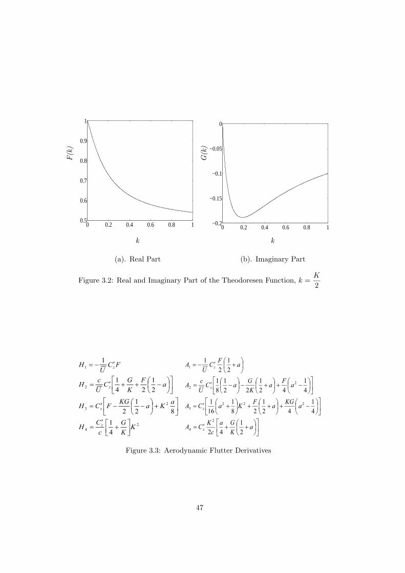
0 0.2 0.4 0.6 0.8 10.5

0.6

0.7

0.8

0.9

1

k

F(k

)

0 0.2 0.4 0.6 0.8 1−0.2

−0.15

−0.1

−0.05

0

k

G(k

)

(a). Real Part (b). Imaginary Part

Figure 3.2: Real and Imaginary Part of the Theodoresen Function, k =K

2

Figure 3.3: Aerodynamic Flutter Derivatives

47

Reissner (1926) analysed the wing torsional divergence demonstrating the impor-

tance of relative locations of the aerodynamic center of pressure and the elastic axis.

The parameter ‘a’ is the dimensionless distance between these two points of inter-

est based on a reference length c/2. In our case a = -1/4 for the symmetric airfoil

and a = 0 for the streamlined bridge deck section. In practice, flutter derivatives of

suspended bridge deck sections are measured experimentally on a case to case basis.

Measurement of the same for the bridge deck section in question is however, out of

the scope of this work.

Numerical Simulations

As stated earlier, Sec.2.3, we used the Fox and Goodwin iteration scheme to nu-

merically solve the governing equations 2.7 and 2.8. We shall use the same scheme

to solve the equation 3.1, 3.5 and 3.6. Results from the numerical simulations shall

be used to validate the measured structural parameters as in Fig.3.5 and Fig.3.10.

The same numerical scheme is used to simulate the theoretic energy curve in Fig.6.14.

The Fox and Goodwin iteration scheme is a modified form of the widely known

single step Newmark iteration method. In our case we shall implement the prediction-

correction strategy in each iteration to solve the equations of motion. Unlike the

standard Newmark scheme, Fox and Goodwin defined the constants as γ =1

2and

β =1

12. Assigning these values improves the precision of the method to the third

order compared to a second order precision level obtained by the standard scheme.

The stability condition in this case is typically defined as ∆tω ≤√

6. The inherent

numerical damping in the scheme is reduced to zero given the fact that the phase

error is shifted to the third order, Geradin & Rixen (1992). We implemented the

Fox and Goodwin scheme using the following algorithm:

Prediction x∗

n+1 = xn + (1 − γ)∆txn

x∗

n+1 = xn + ∆txn + (1

2− β)∆t2xn

Acceleration xn+1 =f(

x∗

n+1, x∗

n+1, tn+1

)

− cx∗

n+1 − kx∗

n+1

1 + cγ∆t + kβ∆t2

Correction xn+1 = x∗

n+1 + γ∆txn+1

xn+1 = x∗

n+1 + β∆t2xn+1

(3.10)

48

3.2 Wind Tunnel Setup and Measurement Techniques

3.2.1 Wind Tunnel Setup

All the experimental results discussed in this study were obtained using the fluid

structure interaction lab facility at the Laboratoire d’Hydrodynamique, (LadHyX).

Experiments were conducted on an airfoil and a bridge deck model separately. The

models are flexibly mounted in an Eiffel type wind tunnel. The wind tunnel has a

test section of 0.18m width. A 2500W centrifugal fan is installed down-stream of the

test section. When operated the fan can create an airflow from ≈ 4m/s to ≈ 30m/s

at maximum power. Air discharge from the fan exhaust is in the vertical direction.

Contraction section of the wind tunnel is 0.5m long. A wire mesh and a honey comb

structure at the inlet of the contraction section ensures a turbulence level of 1.5% at

10m/s.

The models used in the experiments were fabricated using a numerical milling

machine to ensure close dimensional tolerance. The models are suspended in the test

section primarily supported by two long flat Aluminum bands of dimensions 400mm

x 20mm x 2mm. Two sets of vertical springs, one at each extremity of the models

hold them exactly in place. Bending natural frequency of the models is controlled by

adjusting the thickness of Aluminum bands near their clamping positions. Torsional

frequency of the set-ups is controlled by using two sets of horizontal springs on each

side. The models are restrained so that they can oscillate only in the rotational and

vertical degrees of freedom when subjected to an air flow.

It must be pointed out here that there are no moving parts in the experimental

set-ups so that there is no moving friction and the structural damping of the systems

is very low. Sand particles are glued to the leading edge of the airfoil to ensure that

the boundary layer separation takes place always at the same point. End plates were

used to further the two dimensionality of the experimental set-up.

3.2.2 Measurement Techniques

Measurements are obtained using two laser displacement sensors for each degree

of freedom. Measurement resolution used during the course of the experiments is

40µm. The laser sensors have an accuracy better than 1% of the full scale range,

±10mm. Output signals from the laser displacement sensors are treated by a PAK

49

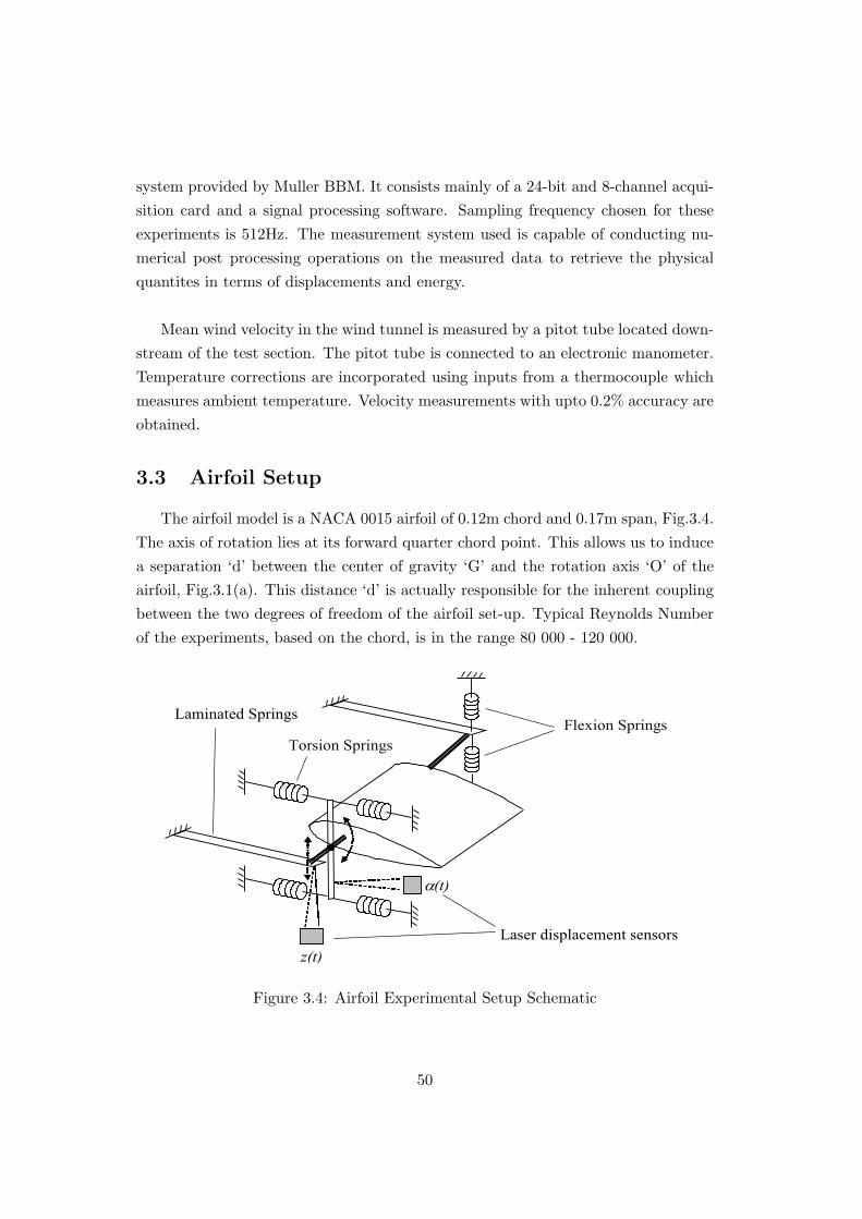
system provided by Muller BBM. It consists mainly of a 24-bit and 8-channel acqui-

sition card and a signal processing software. Sampling frequency chosen for these

experiments is 512Hz. The measurement system used is capable of conducting nu-

merical post processing operations on the measured data to retrieve the physical

quantites in terms of displacements and energy.

Mean wind velocity in the wind tunnel is measured by a pitot tube located down-

stream of the test section. The pitot tube is connected to an electronic manometer.

Temperature corrections are incorporated using inputs from a thermocouple which

measures ambient temperature. Velocity measurements with upto 0.2% accuracy are

obtained.

3.3 Airfoil Setup

The airfoil model is a NACA 0015 airfoil of 0.12m chord and 0.17m span, Fig.3.4.

The axis of rotation lies at its forward quarter chord point. This allows us to induce

a separation ‘d’ between the center of gravity ‘G’ and the rotation axis ‘O’ of the

airfoil, Fig.3.1(a). This distance ‘d’ is actually responsible for the inherent coupling

between the two degrees of freedom of the airfoil set-up. Typical Reynolds Number

of the experiments, based on the chord, is in the range 80 000 - 120 000.

Figure 3.4: Airfoil Experimental Setup Schematic

50

3.3.1 Structural Parameters

Structural parameters are identified for each pure degree of freedom taken inde-

pendently under zero wind velocity using Eqn.3.4 and Eqn.3.5. Computations curve

in Fig.3.5 is obtained by numerically simulating Eqn.3.1. The technique used for

simulations is described in Sec.3.1, Eqn.3.10.

−3

−2

−1

0

1

2

3

0 0.5 1 1.5 2 2.5 3−4

−2

0

2

4x 10

−4

Time(s)

z(t)

α(t

)

Figure 3.5: Time evolution of angular and bending displacement, Initial conditions:αo = −2.173o, zo = −0.0003534m. Linear Airfoil Setup (Table 3.1). (solid-line)Experiment, (dashed-line) Computation.

3.3.2 Critical Velocity

The most important parameter relative to the long term study of such fluid

structure interaction systems is the critical velocity. If the incident wind velocity

approaches this value, the system may suffer from the flutter instability. In order

to demonstrate the calculation of critical velocity, following Hemon et al. (2006),

51

we shall start by rewritting Eqn.3.1, this time identifying the added aerodynamic

damping terms:

z + 2 (ηz + ηaz)ωz z + kzz + dα =Fz

m

α + 2 (ηα + ηaα)ωαα + kαα +md

Jo

z =Mo

Jo

(3.11)

combining with Eqn.3.7 and applying the quasi-steady hypothesis, we have the

following form:

z + 2 (ηz + ηaz)ωz z + ω2zz + dα =

ρbcU2r

2cf2z m

C ′

zα

α + 2 (ηα + ηaα)ωαα + ω2αα +

md

Jo

z = 0

(3.12)

considering the system in Eqn.3.12 without any damping:

z + ω2zz + dα =

ρbcU2r

2cf2z m

C ′

zα

α + ω2αα +

md

Jo

z = 0

(3.13)

if the eigen values of such a system become complex, natural frequencies of the

two degrees of freedom shall become equal and the airfoil shall experience flutter.

Mathematically,

det

∣

∣

∣

∣

∣

∣

∣

λ − λz λd +ρbcU2

r

2cf2z m

H3

λmd

Jo

λ − λα

∣

∣

∣

∣

∣

∣

∣

= 0 (3.14)

now, we can find the smallest root U2 of the following second order equation:

(

λz + λα +dρbcU2

2Jo

C ′

z

)2

− 4λzλα

(

1 − md2

Jo

)

= 0 (3.15)

the critical velocity is now given by:

U2c =

−2Jo

(

− (λz + λα) +

√

4λzλαλz + λα

λ1 + λ2

)

dρbcC ′

z

(3.16)

52

Using the system parameters as catalogued in Table 3.1, we solve the Eqn.3.16 for

Uc which is found to be 18.58 m/s for this case.

3.3.3 Frequency

Normalized frequencies of the two degrees of freedom are shown in Fig.3.6. We

can see that the two frequencies approach one an other as the incident mean wind

velocity increases. The two frequencies finally merge at the critical velocity sig-

nalling the on-set of the flutter instability. This value of the flutter frequency can

be calculated using

f2c =

1

(2π)2

√

λzλαλ1 + λ2

λz + λα(3.17)

substituting values in Eqn.3.17, we obtain the critical frequency value, fc = 5.99Hz.

This value is normalized with respect to the bending natural frequency fz giving a

dimensionless value 1.21, marked by the dashed line in Fig.3.6.

0 0.2 0.4 0.6 0.8 10.6

0.8

1

1.2

1.4

1.6

1.8

U

Uc

f 1 f z

f 2 f z

Figure 3.6: Frequency Ratios of the 2 modes versus velocity parameter; Schwartzet al. (2009).

53

3.3.4 Aerodynamic Damping

We know that aerodynamic damping plays a very important part in over all sys-

tem dynamics. In order to fully observe the contribution of aerodynamic phenomena

in the overall damping of the system, each degree of freedom is studied independently,

Fig.3.7. The experimental setup was designed to keep the two structural dampings

as low as possible. Applying the quasi-steady conditions, we know that the pure

aerodynamic damping for each degree of freedom can be written as:

H1 =−1

UC ′

z ; A2 =−1

8

c

UC ′

z (3.18)

These aerodynamic dampings can be rewritten in a direct form by exploiting

Eqns.3.1, 3.7 and 3.18 as follows:

ηaz=

ρbcU

4mωz

C′

z ; ηaα=

ρbc3U

32Joωα

C′

z(3.19)

C′

z was measured and found to be approximately equal to 2π. Aerodynamic

damping curves obtained from Eqn.3.19 are compared with the experimental findings

in Fig.3.7. Good agreement between the experimental points and the damping curves

obtained by the quasi-steady theory validates the experimental procedure and the

identification of structural parameters.

54

0 5 10 15 200

0.5

1

1.5

2

2.5

3

U (m/s)

η az

0 5 10 15 200

0.5

1

1.5

2

2.5

3

U (m/s)

η aα

Figure 3.7: Aerodynamic damping versus velocity; (o) Experiment; (-) QST. LinearAirfoil Case (Table 3.1).

Table 3.1: Airfoil System Parameters

kα, kz 1.66 ± 0.05 881 ± 33 (N.m/rad) , (N/m)

g 0.655 ± 0.04 mm

δk 120 ± 5 N/m

b, c 0.12 ± 0.0001 0.17 ± 0.0001 m

fα, fz 6.9375 ± 0.0625 4.9375 ± 0.0625 Hz

f1, f2 4.9375 ± 0.0625 7.4375 ± 0.0625 Hz

ηα, ηz 0.2 ± 0.01 0.15 ± 0.01 (%)

Jo, m 8.74e−4 ± 0.25e−4 0.915 ± 0.05 (kg.m2), (kg)

d 9.3 ± 0.3 mm

55

3.4 Bridge Deck Setup

The bridge deck section has a chord, B = 0.11 m and a span 0.17 m. The

bridge deck model is supported at its axis of rotation which is located at its chord-

wise geometric center, Fig.3.1(b). Bridge deck model mimicks the cable-stayed road

bridge constructed over the valley of river Tarn near Millau in Southern France,

Fig.3.8. Typical Reynolds number of the experiments, based on the chord, is in the

range 35 000 - 160 000.

Figure 3.8: Bridge Deck Cross Section Schematic.

56

Figure 3.9: Bridge Deck Cross Section Schematic.

57

3.4.1 Structural Parameters

Structural parameters are identified for each pure degree of freedom taken inde-

pendently under zero wind velocity using Eqn.3.4 and Eqn.3.5. Total energy is the

sum of the system’s Kinetic and Potential energies, Eqn.3.6 for bridge deck setup.

−2

−1

0

1

2

0 0.5 1 1.5 2 2.5 30.4

0.6

0.8

1

Time(s)

E(t

)

Eo

α(t

)

Figure 3.10: Time evolution of angular displacement and corresponding dimension-less total energy U = 0, αo = 1.66 , Bridge Deck Section, Case 2 (Table 3.2).(solid-line) Experiment, (dashed-line) Computation.

Measurement of these structural parameters is validated by comparing an exper-

imental test for each case without wind with results from numerical simulation, as

shown in Fig.3.10 for one of the cases. The numerical simulation technique is de-

scribed in Sec.3.1, Eqn.3.10. Initial conditions for each independent case are provided

by small mechanically induced offsets. For the pure vertical displacement case, the

laminated springs also introduce a small angle of rotation. This is taken into account

in the recovery procedure of the laser signal. Close agreement of the experimental

58

and simulation curves in Fig.3.10 verifies the correct detection and measurement of

various structural parameters of the experimental setup.

3.4.2 Frequency Ratio

As part of our experimental investigations of the stream-lined bridge deck section;

three different setups were used. All the three setups are distinctly identifiable on

the basis of their frequency ratios. In this study the frequency ratio is defined as

the ratio of the natural bending frequency of the bridge deck section to the pure

torsional frequency.

rF =fz

fα

(3.20)

0 0.2 0.4 0.6 0.8 10

0.5

1

1.5

2

2.5

3

U

Uc

f 1 f z

f 2 f z

Figure 3.11: Frequency Ratios of the 2 modes versus Velocity Ratio.Case 3, (Table3.2).

Recalling that the system is a Type-II (Class-1), Sec.1.1, Fig.1.1, fluid structure

interaction system; in such two degrees of freedom cases one of the frequencies of the

system remains almost constant while the second frequency changes as a function of

mean free stream velocity. In this particular case, bending frequency (f1) of the sys-

tem remains quasi-constant. Torsional frequency (f2) however changes. As the mean

59

free stream velocity is increased, torsional frequency moves towards the bending fre-

quency until for a certain critical value of wind velocity, the two frequencies merge.

In this result slight dispersion in the experimental points for the bending frequency

can be observed in the vicinity of the critical velocity. A closer data resolution could

not be obtained due to the practical constraints. If however, the velocity is increased

further, the flutter in-stability sets in. The flutter frequency, fc/fz shall be the same

as f1/fz.

Effect of Frequency Ratio on Critical Velocity

In our case for a frequency ratio 0.44, the maximum critical flutter velocity

was 21.34 m/s as shown in Fig.3.12. This maximum velocity is close to maximum

allowable operational velocity of the wind tunnel which is slightly more than 25 m/s.

After credible energy evolution data had been obtained for this case, the system

parameters were changed to obtain a frequency ratio value of 0.62. It is observed,

as in Fig.3.12, that increasing the frequency ratio of the bridge deck section actually

reduced the critical wind speed. Bridge deck systems with a higher frequency ratio

shall have an equally lower critical wind speed making them susceptible to structural

fatigue and a risk of complete failure at much lower incident wind speeds. The

representation, 1−(

fz

fα

)2

, has been adopted to keep in line with Schmid & de Langre

(2003).

Effect of Frequency Ratio on Aerodynamic Stiffness

We know that the aerodynamic added terms including the aerodynamic damping

and aerodynamic stiffness play a very important part in overall system dynamics.

Aerodynamic dampings have been discussed in Sec.3.4.3, Fig.3.14. Aerodynamic

Stiffness, A3# is measured experimentally using the following expression, assuming

that Quasi-Steady Theory holds:

A#3 = K2A∗

3 =

2Joλα

(

1 −(

fz

fα

)2)

ρbB2U2c

(3.21)

where A#3 is inspired from Scanlan’s flutter derivatives for which ‘K’ is the re-

duced angular frequency. Added stiffness is found to be quasi-constant for all the

three frequency ratios. Experimental values of the aerodynamic stiffness are plotted

as a function of the frequency parameter in Fig.3.13.

60

0 0.2 0.4 0.6 0.8 110

12

14

16

18

20

22

24

1 −(

fz

fα

)2

Uc(m

/s)

Figure 3.12: Dimensional Critical System Velocities versus Frequency Ratio; ()Case 1; (O) Case 2; ( ∆ ) Case 3; (Table 3.2)

0 0.2 0.4 0.6 0.8 10

0.5

1

1.5

2

2.5

3

3.5

4

1 −(

fz

fα

)2

A3#

Figure 3.13: A3# versus Frequency Ratio at the respective critical velocities. ()

Case 1; (O) Case 2; (∆) Case 3; (Table 3.2)

61

3.4.3 Aerodynamic Damping

Recalling from Scanlan & Tomko (1977) and Sec.3.1, we know that the Standard

Airfoil Theory as invoked above cannot be reliably used in case of a bridge deck

section irrespective of the surface streamlining conditions. Therefore, for experiments

conducted on the bridge deck section we use simple linear regression to observe the

evolution of added damping with respect to the increasing mean wind velocity. The

added damping is found to evolve linearly as expected from the Quasi-Steady Theory.

Straight line in Fig.3.14 thus, represents the linear regression unlike in Fig.3.7 where

the same is used to represent the Quasi-Steady Theory.

0 5 10 150

0.2

0.4

0.6

0.8

1

1.2

1.4

U (m/s)

η az

0 5 10 150

0.5

1

1.5

2

2.5

U (m/s)

η aα

Figure 3.14: Aerodynamic damping versus velocity; () Experiment; (-) LinearRegression. Bridge Deck Section Case 1 (Table 3.3).

3.5 Discussion

All the experimental results in this chapter have been reasonably validated using

simple theoretical methods. As stated earlier, importance of such procedures cannot

be under estimated for the fact that findings from these experiments shall be used in

the more complicated transient energy growth studies. Any small discrepency can

snowball into an un-acceptable error if proper attention is not paid to the fine details.

62

Table 3.2: Structural Parameters of Different Bridge Deck Sections Studied

fz

fα

fα fz kα kz Jo m ηα% ηz%

Case 1 0.84 8.00 6.75 1.85 1246.91 7.32e−4 0.69 0.17 0.16

Case 2 0.62 7.12 4.43 1.33 519.36 6.64e−4 0.66 0.3 0.08

Case 3 0.44 8.00 3.56 1.67 309.16 6.61e−4 0.62 0.24 0.07

Table 3.3: Measured Parameters of Different Bridge Deck Sections Studied

fz

fα

Uc A#3

Case 1 0.84 12.74 2.53

Case 2 0.62 16.14 2.66

Case 3 0.44 21.34 2.38

63

PART-II Transient Behavior

As the name suggests, this part is reserved for the transient behavior of all the

three fluid structure systems studied in Part-I. As pointed out earlier, Sec.1.4, re-

searchers started paying attention to the existence of transient energy growth in fluid

structure systems very recently. Experimental evidence published lately proves the

existence of this phenomenon. Traditionally, spectral methods have been used to

estimate structural constraints in such problems. However, recent research shows

that such techniques may not always encompass all the exisitng phenomenon arising

due to the combination of wind turbulence excitation and aeroelastic effects. This

scenario becomes increasingly important in situations where a bridge deck may be

exposed to high turbulent wind close to the ground level, for example. It is such real

life scenarios which reflect the need for exhaustive temporal simulations. The time

domain simulation tool enables us to treat wind gusts as a sudden transient exci-

tation instead of a stationary excitation as largely assumed during typical spectral

investigations. A very important favorable consequence of using temporal simula-

tions is the fact that we can detect and study transient energy growth phenomenon

as shall be discussed during the course of this part.

In this part we present an exhaustive experimental study demonstrating the

existence of transient growth and techniques employed to objectively quantify our

findings. Results have been compared with existing theoretical tools where available

and where permitted by the time constraints. We shall start with the investigation of

the transient behavior exhibited by a freely oscillating square cylinder. Growth rate

of oscillations amplitude in the transient regime is measured and presented. Then

we move on to a two degree of freedom bridge deck section studied in a wind tunnel.

We demonstrate how the maximum energy amplification due to transient growth in

such systems can be linked to the frequency ratio and the amplitude of the initial

mechanical excitation. The bridge deck behavior is studied under the effect of both

mechanical excitation and excitation by an upstream gust, separately. These results

are followed by the experimental investigation of a non-linear symmetric airfoil. We

present experimental results showing the by-pass transition to flutter instability due

to transient growth in case of a non-linear airfoil setup. A new combination of

the already existing quasi-steady theory and the Kussner’s aerodynamic admittance

function is proposed to validate the transient energy amplification results obtained

from a linear airfoil setup subjected to an upstream gust. This combination enables

us to circumvent the complex details of standard un-steady airfoil theory.

Chapter 4

Transient Behavior of a Square

Cylinder

Before we go into the details of the transient behavior of the square cylinder, it

is important to keep in mind that we are interested in the long term and transient

behavior of the cylinder in the VIV regime. This vortex induced vibration region is

in turn governed by the extent of the frequency lock-in domain as discussed earlier,

Chapter 2.

Amandolese & Hemon (2010) recently published interesting experimental data

obtained using long time analysis of the limit cycle oscillations. Results presented by

the authors depict that the oscillations frequency tends to approach the vortex shed-

ding frequency at the beginning of the lock-in. As the reduced velocity is increased,

the oscillations frequency increases settling eventually at a value slightly higher than

the natural frequency of the cylinder, Fig.4.1. This frequency coalescence mechanism

as demonstrated by the authors is in line with de Langre (2006) and validates our

earlier discussion, Fig.1.1, Sec.1.1.

4.1 Measurement Procedure

We recall from Fig.2.3 that the square cylinder oscillating under the vortex shed-

ding effect in a wind tunnel actually passes a transient stage before it achieves the

limit cycle oscillations amplitude. One of the most straight forward technique to

quantify the cylinder behavior in the transient regime is to measure the amplitude

68

0 5 10 15 20 25 300.99

0.995

1

1.005

1.01

Ur

F∗

Figure 4.1: Reduced frequency of the LCO versus reduced velocity zoomed aroundthe lock-in region, reproduced as Amandolese & Hemon (2010)

growth rate for each value of up-stream velocity. The logarithmic decrement tech-

nique is used for this purpose. de Langre (2006) reported that the growth rate of

amplitude of a cylinder executing vortex induced oscillations increases during the

frequency lock-in range resulting in a higher oscillation amplitude. These measure-

ments are however possible only for the starting from rest configuration of these

experiments, Fig.2.4.

For each value of the mean free stream velocity, the cylinder is brought to rest

and then allowed to respond to the incident wind. Data accumulation is triggered

manually from as soon as the cylinder is let free untill the cylinder achieves limit

cycle amplitude. Square of the cylinder displacement, z2(t) is plotted on a semi-

logarithmic scale as a function of time, Fig.4.2. Corresponding values of time i.e.

t1 and t2 are noted when the z2(t) curve intersects two consecutive base lines along

the y-axis. We use the logarithmic decrement formula as Eqn.4.1 to calculate the

reduced growth rate, δ(%).

δ(%) = −100ln

1

104πf∆t

(4.1)

69

Figure 4.2: Logarithmic decrement technique used to measure the growth rate.

4.2 Growth Rate in the Transient Region

For the ‘starting from rest’ configuration, Fig.2.4, the transient behavior of the

cylinder oscillation has been characterized by measuring the growth rate of the os-

cillations amplitude.

The growth rate δ(%) has been identified in the VIV regime for reduced velocity

ranging from ≈ 7 up to ≈ 14. Results are reported in Fig.4.3 where the growth

rate is presented (as percentage of the cylinder critical damping) as a function of

the reduced velocity. It must be noted that the growth rate values have not been

corrected by the damping ratio of the cylinder motion in still fluid. To do so and

to express a growth rate due to pure aerodynamics effect one has to subtract the

damping ratio value η = 0.0828% from the growth rate data presented in Fig.4.3.

We can observe from Fig.2.3 that the amplitude of the square cylinder increases

quasi exponentially. Experimental data presented in Figure 4.3 shows a sharp in-

crease at the beginning of the lock-in, with a maximum slightly below 0.2% for a

reduced velocity corresponding to the matching of the oscillations frequency with the

vortex shedding frequency (Ur ≈ 1/St ≈ 8). Beyond, the growth rate then decreases

in a slightly smoother way. This growth-rate behavior is in line with the frequency

70

coalescence results discussed earlier, Fig.4.1. Moreover, the same can be highlighted

using classical couple mode-flutter analysis between the cylinder dynamics and the

wake dynamics as reported in de Langre (2006).

6 7 8 9 10 11 12 130

0.05

0.1

0.15

0.2

Ur

δ%

Figure 4.3: Growth rate of the oscillations (percentage of the critical damping) versusreduced velocity.

It is imperative to note here that contrary to the results presented and discussed

in Sec.2.2, the maximum growth rate lies closer to the expected (1 / St). Hence, the

off-set in the amplitude results cannot be explained by the blockage effect alone. In

order to resolve this, we shall propose continuation of the present research work and

some investigations of the wake-oscillator model in the following chapters.

4.3 Discussion

As emphasized in Chapter 2, our study finds an over all lack of experimen-

tal evidence concerning a square cylinder executing free vortex induced oscillations

subjected to an airflow. Such evidence is needed to support the already existing

theoretical models, de Langre (2006) for example.

71

Chapter 5

Transient Behavior of a Bridge

Deck

5.1 Introduction

A spring mounted bridge deck section with two degrees of freedom is studied in a

wind tunnel, Sec.3.2. The bridge deck profile is restrained such that it can oscillate

only along the flexural and torsional degrees of freedom. Since the profile is hinged

at its center of gravity there is no inherent structural coupling between the two de-

grees of freedom. However, coupling appears in the added aerodynamic terms in

the expression for linear aerodynamic loading in such cases, Sec.3.1, Eqn.3.7. Also,

given the physical structural constraints in the experimental setup, the two degrees

of freedom cannot be mutually isolated. A small off-set in any one of the degrees

of freedom induces a proportional off-set in the other. This fact has been kept in

mind and appropriate algorithms have been implemented for the accquistion and

post processing of experimental data to minimize error.

Experimental evidence is provided linking the frequency ratio, the critical veloc-

ity and the maximum transient energy amplification of a bridge deck section. The

transient growth of energy is found to have significant effects on the behavior of the

bridge deck. Energy amplification reaches up to 5 times the initial energy transmit-

ted by the gust at a mean velocity just below the critical flutter velocity.

An Aluminum flap is used to generate the upstream perturbation which trig-

gers the vertical and torsional oscillations in the flexible bridge deck system. This

72

perturbation is characterized using two component hot wire anemometry. Measure-

ments consist of the time histories of oscillations in the two degrees of freedom using

laser displacement sensors. Structural parameters are estimated without airflow.

Time evolution of energy of the bridge deck section is measured and amplification

is recorded for the deck section, first for a given set of initial conditions and then

under the effect of the upstream perturbation.

It is important to keep in mind that the dynamics and aeroelasticity of a bridge

deck are different from those of an airfoil. Hence, most of the existing theoretical

tools commonly employed to study the airfoil behavior cannot be directly used in

such cases.

Transient Growth

Before we discuss our experimental results in detail, it makes sense that we remind

ourselves of the phenomenon of transient growth. This phenomenon until now has

been a subject of immense scientific investigations in the field of hydrodynamic sta-

bility. Its effects in case of fluid structure systems started attracting some attention

very recently, Schmid & de Langre (2003). It is already widely known that in case

of viscous flows, transition to an unstable state is possible if an initial disturbance

grows to activate any non-linear mechanisms in the system under consideration. In

this thesis report however, we shall restrict our focus to the transient energy growth

essentially in case of fluid structure interaction systems.

Let us start by considering any linear fluid structure system with coupled two

degrees of freedom. In the absence of any external excitation the system tends to

preserve its equilibrium state. Assuming now that at time to the system is excited

using an external dynamic variable, incident wind for example. The system achieves

an energy state Eo. If the system is stable the energy Eo decays with the passage of

time and the system returns to its equilibrium state, Fig.5.1(a). On the other hand

in case if the magnitude of the external excitation is beyond the linear stability limit,

energy of the system grows exponentially in response ultimately resulting in system

failure, Fig.5.1(b). In our experiments using linear models, the stability limit can be

accurately known by measuring the critical velocity.

In real life scenarios however, the fluid structure interaction mechanism is not

as simple. Speaking strictly of a solid object subjected to an incident airflow, if the

73

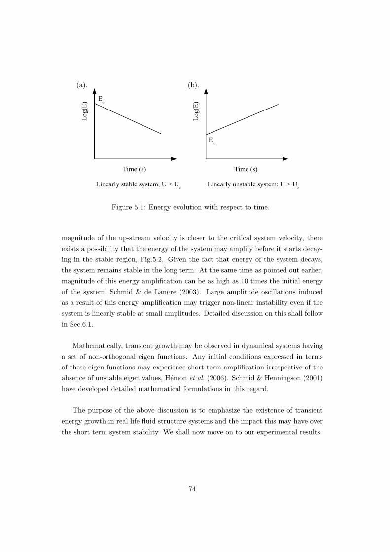
(a). (b).

Figure 5.1: Energy evolution with respect to time.

magnitude of the up-stream velocity is closer to the critical system velocity, there

exists a possibility that the energy of the system may amplify before it starts decay-

ing in the stable region, Fig.5.2. Given the fact that energy of the system decays,

the system remains stable in the long term. At the same time as pointed out earlier,

magnitude of this energy amplification can be as high as 10 times the initial energy

of the system, Schmid & de Langre (2003). Large amplitude oscillations induced

as a result of this energy amplification may trigger non-linear instability even if the

system is linearly stable at small amplitudes. Detailed discussion on this shall follow

in Sec.6.1.

Mathematically, transient growth may be observed in dynamical systems having

a set of non-orthogonal eigen functions. Any initial conditions expressed in terms

of these eigen functions may experience short term amplification irrespective of the

absence of unstable eigen values, Hemon et al. (2006). Schmid & Henningson (2001)

have developed detailed mathematical formulations in this regard.

The purpose of the above discussion is to emphasize the existence of transient

energy growth in real life fluid structure systems and the impact this may have over

the short term system stability. We shall now move on to our experimental results.

74

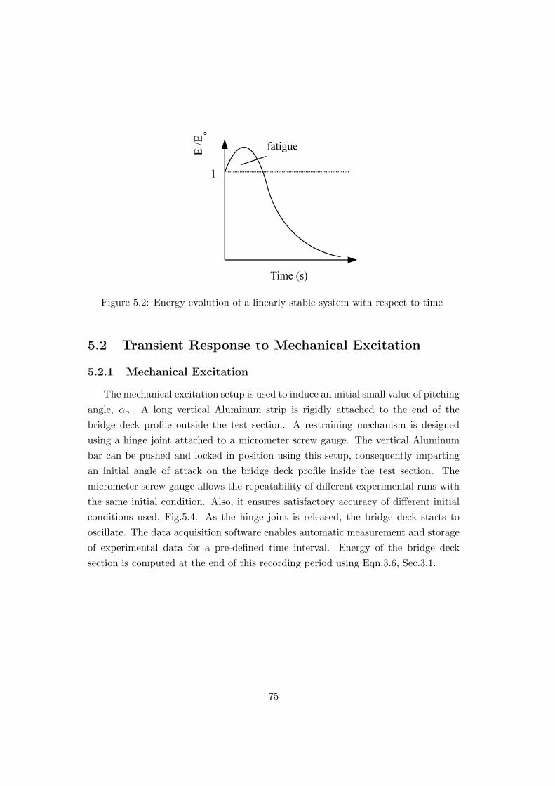
Figure 5.2: Energy evolution of a linearly stable system with respect to time

5.2 Transient Response to Mechanical Excitation

5.2.1 Mechanical Excitation

The mechanical excitation setup is used to induce an initial small value of pitching

angle, αo. A long vertical Aluminum strip is rigidly attached to the end of the

bridge deck profile outside the test section. A restraining mechanism is designed

using a hinge joint attached to a micrometer screw gauge. The vertical Aluminum

bar can be pushed and locked in position using this setup, consequently imparting

an initial angle of attack on the bridge deck profile inside the test section. The

micrometer screw gauge allows the repeatability of different experimental runs with

the same initial condition. Also, it ensures satisfactory accuracy of different initial

conditions used, Fig.5.4. As the hinge joint is released, the bridge deck starts to

oscillate. The data acquisition software enables automatic measurement and storage

of experimental data for a pre-defined time interval. Energy of the bridge deck

section is computed at the end of this recording period using Eqn.3.6, Sec.3.1.

75

2 2.5 3 3.5 4 4.5 5 5.5 60

1

2

2 2.5 3 3.5 4 4.5 5 5.5 6−5

0

5

2 2.5 3 3.5 4 4.5 5 5.5 6−4

−2

0

2

4x 10

−3

Time (s)

α(t

)z(t

)E

(t)

Eo

Figure 5.3: Time Evolution of Energy, Angular Displacement and Vertical Displace-ment of the Bridge Deck Section. Mechanical Excitation. U/Uc = 0.8 , Case 2,[Initial Conditions: αo = −2.212 ; zo = −0.0009191] (Table 3.3).

76

The transient response of the bridge deck system due to the initial mechanical

excitation can be observed from Fig.5.3. Transient response of the bridge deck

sections is depicted as the maximum amplified energy at each value of up stream

velocity normalized by a value of initial energy, Eo. In the present case, this value is

deduced from the initial condition produced by the imposed initial pitch angle, αo.

5.2.2 Effect of Excitation Amplitude

The effects of changes in the initial conditions on the maximum energy amplifica-

tion are presented in Fig.5.4. A slight dispersive effect can be observed as the velocity

approaches the critical velocity of the system or as the velocity ratio approaches 1. It

can be deduced from Fig.5.4 that initial conditions with greater magnitudes result in

a greater energy amplification of the system. Schmid & de Langre (2003) state that

amplifying the initial perturbations may introduce non-linear effects. In the present

study however, magnitude of the initial mechanical excitation is varied within a very

small range i.e. ≈0.8 . The system is safely assumed to behave linearly for different

initial conditions within this range. Hemon et al. (2006) have also studied the effect

of initial conditions on the transient amplification of energy but in case of a linear

two dimensional airfoil in a wind tunnel. Figures 5.5 & 5.6 show sets of experimental

data points obtained from a number of series to validate the reliability of the ex-

perimental technique under similar initial conditions between distinct experimental

series.

77

0.3 0.4 0.5 0.6 0.7 0.8 0.9 11

1.5

2

2.5

3

3.5

4

4.5

5

5.5

U

Uc

Em

ax

Eo

Figure 5.4: Amplification rate of energy versus velocity parameter for Case 2 (Table3.2); (O) αo = −2.6o ; () αo = −2.5o ; ( ∆ ) αo = −1.8o ; (+) αo = −2.1o;Mechanical Excitation

0.3 0.4 0.5 0.6 0.7 0.8 0.9 11

1.2

1.4

1.6

1.8

2

2.2

2.4

2.6

2.8

U

Uc

Em

ax

Eo

Figure 5.5: Amplification rate of energy versus velocity parameter for Case 1 (Table3.2); Mechanical Excitation

78

0.3 0.4 0.5 0.6 0.7 0.8 0.9 11

1.5

2

2.5

3

3.5

4

4.5

5

5.5

U

Uc

Em

ax

Eo

Figure 5.6: Amplification rate of energy versus velocity parameter for Case 3 (Table3.2); Mechanical Excitation

79

5.2.3 Effect of Frequency Ratio

The ‘frequency ratio’ for this experimental study has been defined in Sec.3.4.2.

Although the energy evolution curves for all the three cases of frequency ratios

exhibit similar behavior however, all the three cases manage to attain three different

maximum amplification values. Figure 5.7 shows that as the frequency ratio of the

bridge deck section is increased, the maximum attainable energy amplification just

below the critical upstream velocity decreases. It must be kept in mind that varying

the frequency ratio automatically changes the flutter critical velocity of the bridge

deck. Higher energy amplification for lower frequency ratio can be attributed to

the corresponding higher dimensional value of the flutter critical velocity, Tab.3.3

& Fig.3.12. At the same time, a simple law like a linear evolution of the maximum

energy amplification as a function of the square of the critical flutter velocity could

not be established using these experimental results.

0 0.2 0.4 0.6 0.8 12

2.5

3

3.5

4

4.5

5

5.5

6

1 −(

fz

fα

)2

(

Em

ax

Eo

)

c

Figure 5.7: Maximum Energy Amplification versus Frequency Ratio. () Case 1;(O) Case 2; ( ∆ ) Case 3; (Table 3.2)

5.3 Gust Generation and Identification

In order to study the transient behavior of the system closer to the physical real

world, a gust generating mechanism was incorporated in the experimental set-up.

80

Since in nature, gusts are not a harmonic entity, the aim was to generate a short

singular gust up-stream of the test section and study the system transient behavior

under the effect of this gust. An Aluminum flap (170mm x 45mm) was used. The

flap is mounted on the floor of the wind tunnel. Initially, the flap remains aligned

to the flow direction under the effect of a pre-tensioned spring. A rubber pad at

the edge of the flap damps out vibrations due to impact with the wind tunnel floor

and prevents the flap from bouncing. An accelerometer is attached to the flap. As

the flap is let go by releasing the spring, signal from the accelerometer triggers the

transient data accumulation. This approach ensures that the data is accumulated

from the same relative time instant in each repetition of the experiment. Abrupt

movement of the flap creates a short impulse (u(t), w(t)) which is added to the mean

free stream flow, U , Sec.6.4.1.

0.5

1

1.5

0 0.02 0.04 0.06 0.08 0.1−0.2

−0.1

0

0.1

0.2

Time (s)

w(t

)

U

U+

u(t

)

U

U + umax

U

wmax

U

wmin

U

Figure 5.8: Measured Sample of Upstream Velocity Perturbation.

This impulse was calibrated using two component hot wire anemometry in an

empty test section at the leading position of the bridge deck. The impulse thus cre-

ated has a typical duration period of 0.02s which is below the typical period of the

two degrees of freedom of the bridge deck set-up. For mean wind velocity greater

than ≈ 12m/s, we note that the gust components remain quasi-constant. It may

also be noted that the gust profile generated by this experimental setup agrees to

81

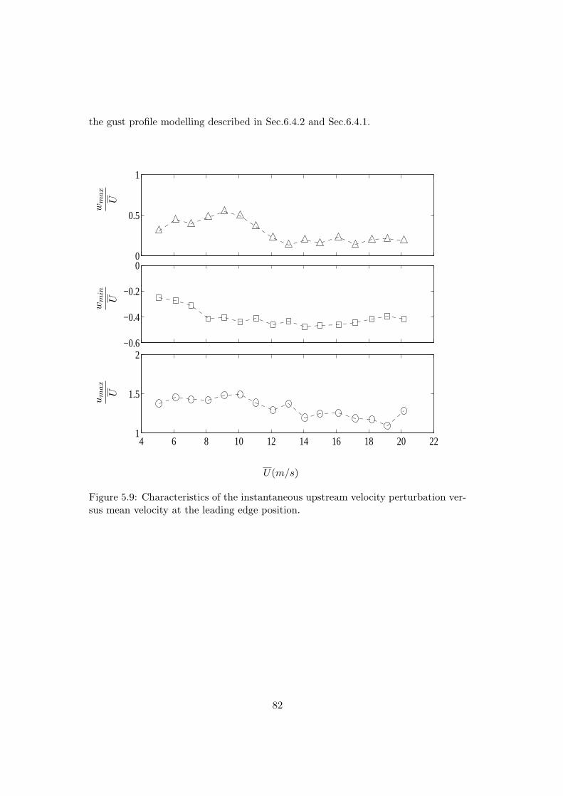
the gust profile modelling described in Sec.6.4.2 and Sec.6.4.1.

0

0.5

1

−0.6

−0.4

−0.2

0

4 6 8 10 12 14 16 18 20 221

1.5

2

U(m/s)

um

ax

U

wm

in

U

wm

ax

U

Figure 5.9: Characteristics of the instantaneous upstream velocity perturbation ver-sus mean velocity at the leading edge position.

82

5.4 Transient Response to Gust Excitation

In the preceding sections we presented our findings from a series of experiments

on a bridge deck section in a wind tunnel. The bridge deck system was excited me-

chanically while the wind velocity remained constant through out the interval of data

accumulation. In this section we shall discuss results obtained from a more realistic

bridge deck experimental setup involving up-stream gust. This gust impulse sets the

system to oscillate upon interaction. We know from Sec.5.3 that the reduced gust

components behave quasi-constantly for mean velocity greater than approximately

12m/s. However, out of the three bridge deck models studied, two have their veloc-

ity range greater then 12m/s, Tab.3.3. We shall therefore, discuss transient growth

results for bridge deck models with velocity range greater than 12m/s.

As obvious in Fig.5.10 there is a clear wedge in the energy curve just before

three seconds. Position of the wedge on the energy curve corresponds roughly with

the maximum pitch and minimum plunge position of the bridge deck section. Total

energy curve of the bridge deck model is normalized using the value at this point

consequently setting it to 1.

A closer observation of Fig.5.3 and Fig.5.10 shall reveal that the gust excita-

tion mechanism generates slightly different transient dynamics when compared with

mechanical excitation. It can be seen that the maximum energy level for both the

cases is achieved for different motion conditions. For mechanical excitation, Fig.5.3,

the maximum energy amplification is obtained for almost a mximum pitch and min-

imum plunge. For the gust excitation however, the maximum energy is obtained

with almost a mimimum pitch and maximum plunge.

83

0

1

2

3

−5

0

5

2 2.5 3 3.5 4 4.5 5 5.5 6−5

0

5x 10

−3

Time (s)

α(t

)z(t

)E

(t)

Eo

Figure 5.10: Time Evolution of Energy, Angular Displacement and Vertical Displace-ment of the Bridge Deck Section. Excitation by Flap. U/Uc = 0.91 , Case 3 (Table3.3).

84

12 14 16 18 200

1

2

3

4

5

6

7x 10

−3

U(m/s)

Eo(J

)

Figure 5.11: Value of Normalization Energy (J) versus Mean Velocity (m/s); (o)Case2; (∆) Case 3. (Table 3.2); Excitation by flap.

Figure.5.11 depicts the dimensional values of normalization energy, Eo(J) plot-

ted against the dimensional mean velocity, U(m/s). We can observe that despite the

distinct structural parameters of the two cases, values of Eo(J) collapse perfectly for

the overlapping operational velocity range i.e. between ≈14m/s and ≈16m/s. This

result reinforces the fact that the values of Eo(J) chosen for this set of experiments

are representative of the gust effect at the bridge deck leading edge. Moreover, this

value of initial energy Eo(J) follows an evolution as the square of the mean wind

velocity.

Figure 5.12 shows the energy amplification behavior of two deck section systems

subjected to an upstream gust. Gust monitoring through out the experiments was

carried out as described in Sec.5.3. We see that the transient growth mechanism

amplifies the initial energy of the system by a factor greater than five just below the

linear stability limit. The experimental data points in this case show a considerably

lesser cohesion when compared to the previous experiments conducted using fixed

mechanical excitations. Still, the maximum energy amplification observed in this

case is approximately of the same order as observed previously in case of mechanical

excitations. This case is however closer to the real world scenario. Though the

85

experimental points are easily distinguishable, they follow approximately the same

trend as we move along the horizontal axis.

0.3 0.4 0.5 0.6 0.7 0.8 0.9 11

1.5

2

2.5

3

3.5

4

4.5

5

5.5

U

Uc

Em

ax

Eo

Figure 5.12: Amplification rate of energy versus velocity ratio; (O) Case2; (∆) Case3. (Table 1); Excitation by flap.

5.5 Discussion

This experimental study high lights the fact that suspended bridged decks ex-

posed to turbulent wind conditions are prone to short term instabilities which may

arise due to the transient energy growth in the system. Some authors have lately ad-

dressed the more general case of transient growth in fluid structure systems. Experi-

mental results from this study including maximum energy amplification by transient

growth follow previous theoretical results. We shall discuss some future aspects of

the study in Sec.7.2.

86

Chapter 6

Transient Behavior of a

Non-Linear Airfoil

6.1 Introduction

As the chapter name suggests, two degree of freedom coupled mode flutter of

a symmetric airfoil is studied in a horizontal wind tunnel. A single upstream gust

is used as the source of excitation for the airfoil. In addition to the experimental

setup described in Sec.3.2 the model is modified to introduce a weak non-linearity

in the system stiffness, Sec.6.2.1. Experiments are repeated for both the linear and

non-linear airfoil models and the results are compared to show that the initial energy

in such non-linear systems may get amplified to the un-stable range by the transient

growth even below the linear stability limit of the dynamic system parameters. Vari-

ous existing theoretical tools have been explored and a comparison is developed with

a simple model validating the experimental results.

Non-Linear Systems and By-Pass Transition

In a linear case, transient growth may lead to an initial amplification of energy

which would subsequently decrease as long as the system is under sub-critical con-

ditions. Hemon et al. (2006) have shown that initial amplification of energy in such

cases is strongly dependent on initial conditions. In a non-linear case on the other

hand, if Ucnl < U < Uc; where Ucnl is the non-linear critical mean free stream veloc-

ity and Uc is the linear critical mean free stream velocity; the resultant amplitude

becomes very important, Fig.6.1. A small initial perturbation may not trigger an

instability but a sufficiently large excitation may push the system in the un-stable

87

region even below the linear critical velocity.

In a non-linear case, i.e. when the airfoil support elasticity behaves non-linearly,

the amplitude of the perturbation is an important parameter due to the sub-critical

branch as illustrated in Figure 6.1(b), when the mean velocity is larger than the

non-linear critical velocity Ucnl and below the linear critical velocity Uc. An initial

small perturbation keeps the system in the stable region but for a larger initial per-

turbation, the system state may reach the unstable region, leading to flutter even

below Uc. This scenario is called by-pass transition to flutter by amplitude effect.

Another possibility is the scenario when the transient growth results in the lin-

ear amplification of an initially small perturbation because the mean velocity is just

below the linear critical velocity. As illustrated in Figure 6.1(c), two possibilities

can exist. The transient amplification remains small and keeps the system stable,

referred to as type B in Figure 6.1(c) or the transient amplification is such that the

system response then reaches the sub critical branch, flutter instability is triggered

(referred to as type C).

The latter is also a by-pass transition to flutter, but caused by transient growth

of a small initial perturbation, the level of which would have lead to stability without

this amplification. It is therefore different from a classic by-pass transition where

the initial amplitude alone triggers the flutter instability. A similar mechanism is a

possible scenario in the domain of transition to turbulence, Schmid & Henningson

(2001).

88

(a).

(b).

(c).

Figure 6.1: (a). Effects of an initial perturbation for a linear system; (b). Perturba-tion amplitude effect for a non-linear system; (c). Scenario of by-pass transition dueto transient growth of an initial perturbation, Schwartz et al. (2009).

89

6.2 Experimental Techniques

6.2.1 Non-Linear Airfoil Setup

The non-linearity is located on the stiffness of the flexion due to the contact

springs. Two parameters are needed, the gap ‘g’ between the position zero and the

contact, and the resulting stiffness knl = kz + δk above this gap. In fact the non-

linear system can be seen as a bi-linear system and the contact springs stiffness was

chosen small enough so that the non-linearity is relatively small. The calibration

Figure 6.2: Kinematics of the flexible airfoil Schwartz et al. (2009).

is performed statically. This leads to a gap value g = 0.655 mm and an additional

stiffness δk = 0.136kz. The non-linear feature of the flexural stiffness leads to an

additional term on the energy that reads:

Enl(t) =δk

4

(

(|z − g| + (z − g))2 + (|z + g| − (z + g))2)

(6.1)

This quantity is added to the energy, Eqn.3.5, when measurements are performed

with the non-linear system.

90

6.2.2 Gust Generation and Identification

It is important to note here that the wind tunnel apparatus used in these exper-

iments is different from the one used for bridge deck experiments, Chapter.5. The

wind tunnel test section has been changed resulting in a corresponding new flap

mechanism. We therefore discuss the results of the gust identification procedure for

the sake of clarity and scientific consistency. Like the previous experimental setup an

Aluminum flap is mounted on the test section floor 160mm up-stream of the airfoil.

Two component hot wire anemometry is used to characterize the impulse, Sec.5.3.

Horizontal component u(t) of the impulse comprises of a unique positive peak. The

vertical component however, has a negative peak followed by a simultaneous posi-

tive peak. An example of the time evolution of both the orthogonal components is

shown in Fig.6.3. It may be noted that the gust profile generated by this experi-

mental setup agrees to the gust profile modelling described in Sec.6.4.1 and Sec.6.4.2.

Figure 6.3: Gust Profile, Schwartz et al. (2009).

Effects of any changes in the mean velocity U , on the behavior of the two com-

ponent velocities are also investigated in Fig.6.4. These characteristic parameters

of the upstream perturbation have been measured in the empty test section at the

91

position of the airfoil leading edge. The impulse thus created has a typical duration

period of 0.05s which is below the typical period of the two degrees of freedom of

the airfoil set-up. A comparison of the accelerometer and the hot wire signals gives

us the time taken by the gust impulse to reach the leading edge of the airfoil. If

the mean free stream velocity, U is maintained at 17m/s, the impulse takes 0.08s

to reach the leading edge of the airfoil. This time interval decreases as the wind

velocity increases in the test section. The gust parameters have been normalized

with respect to the mean wind velocity in the test section.

0

0.4

0.8

−0.4

0.2

0

8 10 12 14 16 18 20 221.2

1.3

1.4

1.5

1.6

U (m/s)

wm

ax

U

wm

in

U

um

ax

U

Figure 6.4: Instantaneous up-stream gust versus mean velocity at the leading edgeposition, Schwartz et al. (2009).

92

6.3 By-Pass Transition due to Transient Growth

The experimental results are mainly presented by comparing the behavior of the

linear system, type A and behaviours of the non linear system, type B or C, Fig.6.1.

The first measured quantities are the periods of the system and their evolution

versus the wind velocity as presented in Figure 6.5 in terms of frequencies. The

linear critical velocity Uc has been previously estimated by experiments, Sec.3.3.2.

In the non-linear system, the period depends on the amplitude of the motion. For

the period measurements, plunge amplitude was then initiated manually during the

recording so that the contact springs were always engaged. Since the gap ‘g’ is small,

the amplitude necessary to reach contact remains small, of the order of 1mm. As

the system is in fact weakly non-linear, the resulting period can be considered as a

mean value between a linear system having a stiffness kz and another linear system

having a stiffness knl = kz + δk, with less than 14% between them. This effect can

be observed at U = 0 where the non-linear system plunge frequency is just above

that of the linear system (5.0625 Hz against 4.9375 Hz).

In the linear system at the onset of flutter the two frequencies coalesce. In the

non-linear case, the coalescence of the two frequencies occurs at a velocity Ucnl which

is lower than in linear case. For a velocity above Ucnl and below Uc a by-pass tran-

sition to flutter is therefore possible.

All data for the transient growth of energy is collected and finally presented in

Figure 6.6, for the linear case, type A, and the non-linear cases, types B and C. The

region covered by the unstable behavior of type C is shown with hachure. When the

system is unstable the motion amplitude grows rapidly and it is stopped manually

as the setup is not designed for high amplitude limit cycle oscillations.

Just below critical velocity with the linear system, the type A presents an ampli-

fication level that is 9 times the value of initial energy. With the non-linear system,

the behavior follows the evolution of the linear system for low velocity. Then, ap-

proaching the value Ucnl, the energy growth rate is higher than in linear case and

finally transition to flutter occurs, after an amplification larger than 7.

The comparison between linear and non-linear behavior is essential for the confir-

mation of the by-pass transition due to transient growth, because this is not a simple

93

0 0.2 0.4 0.6 0.8 14

4.5

5

5.5

6

6.5

7

7.5

8

U

Uc

Fre

quen

cies

(Hz)

Figure 6.5: Frequencies of the 2 modes versus velocity parameter; (o) linear case;(∆) non-linear case. Schwartz et al. (2009).

by-pass transition by initial amplitude effect. The initial perturbation produced by

the flap generates a value of the energy which remains below the level of the energy

for which the non-linear behavior occurs, i.e. the plunge ‘z’ remains below the value

of ‘g’ at the initial instant.

This is shown in Figure 6.7 where we present time histories of the total energy

in a linear case of type A and a non-linear unstable case of type C. Wind velocity

is just below the linear critical velocity: the system is stable for the linear case, and

by-pass transition to flutter occurs for the non-linear case. Before the perturbation

is introduced, the background energy level is of the order 10−5J , a level where the

linear system returns to the stable condition. The initial perturbation of level Eo

is amplified by transient growth up to Emax for the linear case, while it triggers

flutter in non-linear case. In the latter, the boundary of the non-linear behavior was

determined statically. This energy level corresponds to the potential energy of the

system when the displacement ‘z(t)’ reaches the value of ‘g’. Beyond this gap, the

contact springs are engaged and contribute to the stiffness of the airfoil, the system

behaves non-linearly.

94

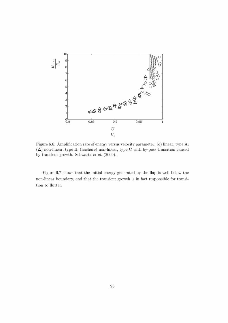
0.8 0.85 0.9 0.95 10

1

2

3

4

5

6

7

8

9

10

U

Uc

Em

ax

Eo

Figure 6.6: Amplification rate of energy versus velocity parameter; (o) linear, type A;(∆) non-linear, type B; (hachure) non-linear, type C with by-pass transition causedby transient growth. Schwartz et al. (2009).

Figure 6.7 shows that the initial energy generated by the flap is well below the

non-linear boundary, and that the transient growth is in fact responsible for transi-

tion to flutter.

95

Figure 6.7: Energy time histories in linear and non-linear cases atU

Uc

= 0.99, Re-

produced from Schwartz et al. (2009).96

6.4 Theoretical Modeling

6.4.1 Gust Modeling

The atmospheric turbulence models can generally be categorized within two dif-

ferent approaches. The methods associated with a discrete gust representation are

generally deterministic in nature. On the other hand, continuous turbulence models

allow for a stochastic perspective. Hybrid methods also exist and are used in some

cases such as the statistical discrete gust, Poirel & Price (1997).

Taylor and Von Karman pioneered the theory of isotropic stochastic turbulence.

Isotropic implies that the properties of air are independent of the orientation at any

point in space. The atmosphere is usually assumed to be homogeneous. Following

Poirel & Price (1997), we assume that by superimposing a mean free stream velocity

U on a fluctuation field, (u, v, w), we can neglect the temporal gradients of turbulent

velocity fluctuations for a coordinate system attached to the mean velocity (x, y, z, t).

This is known as the Taylor’s Hypothesis or The Frozen Gust Assumption. Now,

since the temporal gradients are neglected, a transformation from a spatial to a time

system of coordinates is permissible. For example the longitudinal component with

a mean free stream velocity along the x-axis gives:

u (x, y, z, t) = u (x, y, z) = u(

x − Ut, y, z)

(6.2)

where x, y and z form the body fixed system of coordinates. Hence at any fixed

point on the airfoil, the longitudinal gust is considered as a function of time only.

In two dimensional flows, we consider only the vertical and longitudinal compo-

nents of atmospheric turbulence velocity field. The vertical component acts as an

external forcing function. On the contrary, the longitudinal turbulent field excita-

tion also known as Head on Turbulence, is parametric as it acts on the airspeed.

Furthermore, the gust is assumed to interact with the airfoil in a uniform fashion

in the span wise direction to eliminate the three dimensional complexities from the

model. Any irregularities along the vertical axis are also neglected.

The vertical and the horizontal components in this case were defined using the

standard Gaussian Distribution Functions. The horizontal component is a symmetric

gauss distribution function:

97

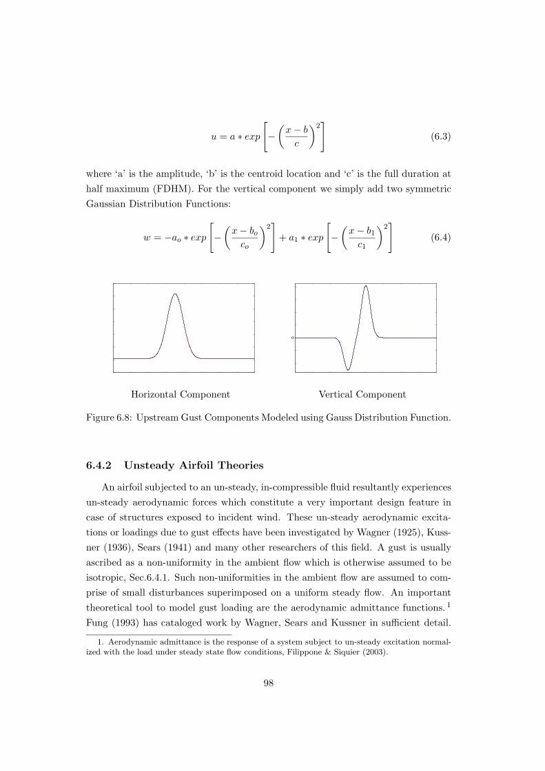
u = a ∗ exp

[

−(

x − b

c

)2]

(6.3)

where ‘a’ is the amplitude, ‘b’ is the centroid location and ‘c’ is the full duration at

half maximum (FDHM). For the vertical component we simply add two symmetric

Gaussian Distribution Functions:

w = −ao ∗ exp

[

−(

x − bo

co

)2]

+ a1 ∗ exp

[

−(

x − b1

c1

)2]

(6.4)

0

Horizontal Component Vertical Component

Figure 6.8: Upstream Gust Components Modeled using Gauss Distribution Function.

6.4.2 Unsteady Airfoil Theories

An airfoil subjected to an un-steady, in-compressible fluid resultantly experiences

un-steady aerodynamic forces which constitute a very important design feature in

case of structures exposed to incident wind. These un-steady aerodynamic excita-

tions or loadings due to gust effects have been investigated by Wagner (1925), Kuss-

ner (1936), Sears (1941) and many other researchers of this field. A gust is usually

ascribed as a non-uniformity in the ambient flow which is otherwise assumed to be

isotropic, Sec.6.4.1. Such non-uniformities in the ambient flow are assumed to com-

prise of small disturbances superimposed on a uniform steady flow. An important

theoretical tool to model gust loading are the aerodynamic admittance functions. 1

Fung (1993) has cataloged work by Wagner, Sears and Kussner in sufficient detail.

1. Aerodynamic admittance is the response of a system subject to un-steady excitation normal-ized with the load under steady state flow conditions, Filippone & Siquier (2003).

98

Response of an airfoil subjected to an upstream gust is studied under the assump-

tions outlined in Fung (1993).

Wagner’s function enjoys fundamental significance in the Unsteady Airfoil The-

ories. The function models circulation growth or lift about an airfoil starting from

rest and reaching a certain uniform velocity with a small angle of attack. The situa-

tion can be accurately modelled using a single step function, Fig.6.9. The circulation

growth is assumed to be uniform over the airfoil as it traverses through a two di-

mensional in-compressible fluid. Wagner formulized the circulatory lift as Eqn.6.5:

L(τ) = −2πρbUwΦ(τ) where Φ(τ) = L−1

(

C(−is)

s

)

(6.5)

Φ(τ) is the Wagner’s aerodynamic indicial admittance function. Details of the

modelling procedure for Eqn.6.5 can be consulted in Fung (1993). W. P. Jones

formulated an approximate expression for a two dimensional airfoil. We use the

same expression, Eqn.6.6 to plot the Wagner’s function in Fig.6.9.

Φ(τ) = 1 − 0.165e−0.041τ − 0.335e−0.32τ (6.6)

0 0.1 0.2 0.3 0.4 0.50

2

4

6

8

w (t)

0 100 200 300 400 5000

0.2

0.4

0.6

0.8

1

Φ(τ)

0 0.1 0.2 0.3 0.4 0.50

0.5

1

1.5

2

2.5

F ′(t)1

2ρU2bc

Figure 6.9: Wagner’s Single Step Behavior.

It is imperative to note that the vertical gust component w(t) is plotted as func-

tion of time, the Wagner’s function Φ(τ) is plotted as a function of non-dimensional

time τ and the normalized fluctuating lift component F ′(t) is plotted as a function

99

of time.

We know that gust loading pattern of the simpliest airfoil cannot actually be

modelled by the single step velocity profile in Fig.6.9. However, the significance of

this simple model for theoretical purposes cannot be over stated. A slightly more

accurate representation of a free stream gust is presented in Fig.6.10. We use a

sequence of step functions to model a velocity profile with a negative peak and a

subsequent positive peak. Such a gust profile is closer to real life scenario. Wagner’s

function approximation by W. P. Jones, Eqn.6.6 is used to obtain the fluctuating lift

component in Fig.6.10.

0 0.05 0.1 0.15 0.2−6

−4

−2

0

2

4

6

8

w (t)

0 100 200 300 400 5000

0.2

0.4

0.6

0.8

1

Φ(τ)

0 0.05 0.1 0.15 0.2

−1

−0.5

0

0.5

1

1.5

2

F ′(t)1

2ρU2bc

Figure 6.10: Wagner’s Multi-Step Function Behavior.

Sears (1941) calculated the lift and moment of a rigid airfoil subjected to a

gust with sinusoidal intensity distribution. He modeled lift as a function of reduced

frequency which in turn depends on the ratio of airfoil chord and gust wavelength.

For such a case, the total lift acts at the quarter chord point of the airfoil at all

times. Sears expressions for lift and moment appear in Eqn.6.7:

L = πρcUWeiwtS(k) ; M = Lc

4(6.7)

where S(k) = [J0(k) − iJ1(k)] C(k) + iJ1(k) is Sears Admittance Function based

on C(k), the Theodoresen Circulation Function, Sec.3.1. Substituting the expression

for Theodoresen’s Function and simplifying we have:

100

|S(k)|2 =(

J20 + J2

1

) (

F 2 + G2)

+ J21 + 2J0J1G − 2J2

1F (6.8)

Sinusoidal gust form, typical sears function profile for our case and the resultant

fluctuating lift component are plotted in Fig.6.11. Since, by definition, the Sears

function is a function of reduced frequency, Eqn.6.8, it remains constant for this

case.

0 0.05 0.1 0.15 0.2

−5

0

5

10

w (t)

0 100 200 300 400 5000

0.2

0.4

0.6

0.8

1

S(τ)

0 0.05 0.1 0.15 0.2

−1

0

1

2

3

F ′(t)1

2ρU2bc

Figure 6.11: Sears Function.

Kussner derived an admittance function which provides lift on an airfoil as it pen-

etrates into a sudden vertical gust. Lift induced by a variable gust can be expressed

as a Duhamel integral, Fung (1993):

L(τ) =1

2ρbcU2C ′

z

∫ τ

0

w(σ)

UΨ′(τ − σ)dσ (6.9)

where Ψ is the Kussner’s admittance function. R. T. Jones provided an approximate

expression for two dimensional elliptic airfoils, Eqn.6.10, Fung (1993):

Ψ (τ) = 1 − 0.5e−0.13τ − 0.5e−τ (6.10)

The fluctuating lift force component exerted by the gust is now computed nu-

merically using the Duhamel integral in Eqn.6.9.

101

0 0.05 0.1 0.15 0.2

−5

0

5

10

w (t)

0 100 200 300 400 5000

0.2

0.4

0.6

0.8

1

Ψ(τ)

0 0.05 0.1 0.15 0.2

−1

0

1

2

3

F ′(t)1

2ρU2bc

Figure 6.12: Kussner’s Airfoil Theory.

Fig.6.12 exhibits the vertical component of the up-stream gust as a function of

time, the Kussner function varying with respect to the non-dimensional time, τ and

the normalized fluctuating component of lift force exerted by the gust.

In this section, we have catalogued all the theoretical tools used in common prac-

tise to understand the aerodynamic behavior of an airfoil subjected to an upstream

gust. Without going into the complicated mathematical details we can see from

Sec.6.2.2 and Sec.6.4.1 that the admittance functions proposed by Wagner and Sears

cannot be used in this study. Firstly, because although Wagner’s step assumption

simplifies the problem to a large extent, yet a step function profile cannot be used

to model a gust as observed in these experiments. Moreover, Sears’ admittance for-

mulation is based on the assumption that the gust behaves sinusoidally. This is also

not the case in our experiments. Infact the experimental setup has been designed

essentially to create only a single gust, Sec.5.3. A rubber padding was used on the

flap so that it can be prevented from bouncing which would have created a somewhat

continuous gust form otherwise. Kussner’s admittance formula on the other hand

is developed for the case of an airfoil penetrating a sudden gust which is about the

case in our experiments.

It is for the reasons described above that the linear aerodynamic load model,

Eqn.6.15 in Sec.6.4.1 depicts only the Kussner’s aerodynamic admittance function.

Moreover, results described in Sec.6.5 depict a theoretical curve obtained by plotting

102

Eqn.6.15. The Kussner’s admittance function was incorporated following Eqn.6.9

and Eqn.6.10.

6.4.3 Slender Body and Quasi-Steady Hypothesis

We shall assume that the airfoil can be considered as a ‘slender body’ with re-

spect to its longitudinal axis and that the ‘Quasi-Steady Hypothesis’ holds. Such

hypotheses hold if the characteristic size of the section is small when compared with

the turbulence length scale.

Effect of Upstream Turbulence

Under such circumstances, the forces due to turbulence can be defined as a func-

tion of the turbulence components in one point representative of the section and can

be evaluated defining an instantaneous velocity corresponding to the resultant of the

mean wind velocity and of the turbulence components. Holding the two hypotheses

and assuming that the turbulence components are small with respect to the mean

wind velocity: u(t) << U and w(t) << U . The forces can be separated into a mean

vector F and a fluctuating part F ′(t). Then Eq.6.11:

Fz =1

2ρU

2

acCz (αa)

Mo =1

2ρU

2

ac2CM (αa)

(6.11)

actually has:

Fz = Fz + F ′

z(t)

My = My + M ′

y(t)

(6.12)

Effect of Airfoil Motion

Variations in the coefficients of aerodynamic forces are functions of the angle of

incidence traced by the apparent velocity.

Assuming α is very small in Fig.6.13, simple substitutions in Eqn.6.11 & Eqn.6.12

provides us the following comprehensive form:

103

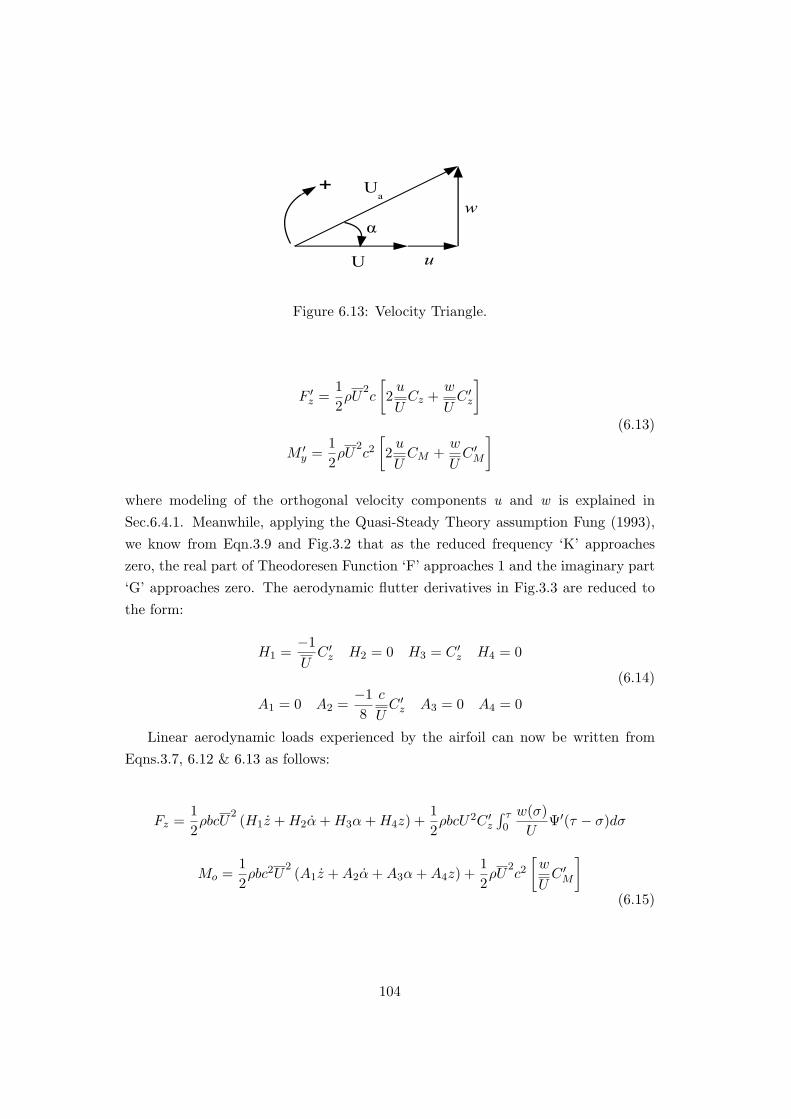
Figure 6.13: Velocity Triangle.

F ′

z =1

2ρU

2c

[

2u

UCz +

w

UC ′

z

]

M ′

y =1

2ρU

2c2

[

2u

UCM +

w

UC ′

M

]

(6.13)

where modeling of the orthogonal velocity components u and w is explained in

Sec.6.4.1. Meanwhile, applying the Quasi-Steady Theory assumption Fung (1993),

we know from Eqn.3.9 and Fig.3.2 that as the reduced frequency ‘K’ approaches

zero, the real part of Theodoresen Function ‘F’ approaches 1 and the imaginary part

‘G’ approaches zero. The aerodynamic flutter derivatives in Fig.3.3 are reduced to

the form:

H1 =−1

UC ′

z H2 = 0 H3 = C ′

z H4 = 0

A1 = 0 A2 =−1

8

c

UC ′

z A3 = 0 A4 = 0

(6.14)

Linear aerodynamic loads experienced by the airfoil can now be written from

Eqns.3.7, 6.12 & 6.13 as follows:

Fz =1

2ρbcU

2(H1z + H2α + H3α + H4z) +

1

2ρbcU2C ′

z

∫ τ

0

w(σ)

UΨ′(τ − σ)dσ

Mo =1

2ρbc2U

2(A1z + A2α + A3α + A4z) +

1

2ρU

2c2

[

w

UC ′

M

]

(6.15)

104

where Ψ (τ) is Kussner’s aerodynamic indicial admittance function which varies with

non-dimensional time, τ =2U

ct, Sec.6.4.2.

6.5 Linear System Experiment versus QST

Circular points in Fig.6.14 represent transient energy growth for the linear airfoil

setup, Sec.3.3. Each circular point denotes the value of maximum energy of the

system normalized with respect to a reference value for each increment in the mean

free stream velocity. We see that as the mean free stream velocity approaches the

linear critical velocity, energy amplification in the system increases exponentially.

It reaches a value of ≈ 9 ≈ 10 for a mean velocity just below the linear critical

velocity. This result is in line with Schmid & de Langre (2003). The authors studied

a generic case of coupled mode flutter and established that energy amplification in

case of linear systems by transient growth mechanism may be as large as 10. For

damped systems, maximum energy amplification scales inversely to the square of the

damping constant, Schmid & de Langre (2003).

0.5 0.6 0.7 0.8 0.9 10

1

2

3

4

5

6

7

8

9

10

U

Uc

Em

ax

Eo

Figure 6.14: Maximum Normalized Energy versus Velocity Parameter. ‘o’ Experi-mental Points, (Solid Line) Computations.

105

Solid line in the figure is obtained by numerically simulating the on-going fluid

structure interaction phenomena using Eqn.6.15. Long term response of the airfoil

can be obtained by the first term on the right hand side in Eqn.6.15. The gust

effect is modelled in the second term including the Kussner’s admittance function.

Normally, such a scenario would have been treated using the full un-steady airfoil

theory. What we propose here is that the long term response of the airfoil can be

reliably predicted using the quasi-steady theory as outlined in Sec.6.4.3. The short

term impulsive response to the up-stream gust can be incorporated into the model

using the Kussner’s admittance function, Eqn.6.9. The important advantage asso-

ciated with this approach is that system dynamics can be studied without going

into the complex mathematical details of the un-steady airfoil theory, Hemon et al.

(2006). The numerical simulation technique used in this case is described in Sec.3.1,

Eqn.3.10. Excitation by the up-stream turbulence effects was modeled using sym-

metric Gauss Distribution Functions as described in Sec.6.4.1.

We can see from Fig.6.14 that although this new combination of the quasi-steady

theory and the Kussner’s admittance formulation slightly under-estimates the max-

imum energy amplification near critical flutter velocity, it models the aeroelastic

phenomena fairly accurately.

6.6 Discussion

Detailed experimental evidence is provided showing the existence of by-pass tran-

sition to flutter instability in case of a non-linear airfoil setup; due to transient

growth. Moreover, a new combination of the standard quasi-steady theory and the

Kussner’s admittance formulation is proposed to model the effects of a single abrupt

gust on a symmetric airfoil. Experimental results and the simulation curve agree

well.

106

Chapter 7

Conclusions and Perspectives

7.1 Conclusions

To conclude, this study deepened our understanding of the transient phenom-

ena in different fluid structure interaction systems. We conducted experiments and

validated our findings using simple theoretical tools. The study emphasizes the

importance of accurate caliberation of different long term system parameters be-

fore they can be used for much complicated short term transient behavior of the

systems. Another important aspect that comes to light is the significance of time

domain simulations necessary for better comprehension of short term energy amplifi-

cation phenomenon. This significance can be attributed to the fact that time domain

simulations allow us to take into account different combinations of the turbulence

excitation and aeroelastic effects. The study allows us to see some inherently com-

plicated phenomena like hysteresis in case of vortex induced oscillations of a bluff

body and the by-pass transition to flutter instability due to transient growth in case

of non-linear airfoil systems.

We started with the vortex induced oscillations of a square cylinder in a wind

tunnel at low wind velocities. An overview of the existing literature shall reveal

that although various authors have written extensively on the underlying mecha-

nisms of vortex induced vibrations, none of the studies caters for a square section

cylinder allowed to respond freely to the incident flow; as is the case in this thesis

report. Experimental set up was designed to ensure nearly two dimensional trans-

verse oscillations. The free vibration approach was chosen due to the lack of existing

experimental evidence for such systems. This approach is closer to a practical real

107

world system due to the fact that it provides direct evidence of non-linear fluid struc-

ture interaction mechanisms as shown and discussed. We conducted the experiments

primarily using two different configurations. In the first case, the square cylinder was

brought to rest for each increment in the upstream velocity. Oscillations growth rate

during the transient phase was measured. In the second case however, the memory

effect was allowed to play for each increment in velocity through out the velocity

range. We were able to capture the ever elusive hysteresis in the reduced amplitude

curve. It is important to underline the fact that although hysteresis is known to ex-

ist, this study is the first of its kind given the unique experimental conditions chosen

for this case. The experimental results were compared with the simulation results of

a theoretical wake oscillator model. Our study shows that while the wake oscillator

model could predict the maximum lock-in amplitude fairly accurately, there remain

some questions regarding the location of the maximum amplitude on the reduced

velocity axis and the extent of the frequency lock-in range. We shall discuss possible

explanations in the next section.

As stated earlier, this study reiterates the importance of the awareness of the

long term behavior of fluid structure systems, indicating its direct implications on

our understanding of the transient behavior of the same. A significant part of this

study is therefore dedicated to the long term system analysis. An efficient exper-

imental setup is proposed capable of generating just a single upstream gust which

can be measured and incorporated into the theoretical model using simple algebraic

tools. Special attention was paid to the fact that structural damping in the exper-

iments remains very low. Sliding friction was eliminated by avoiding any moveable

parts from the setups. Important structural parameters are measured and verified

using simple theoretical tools. We observed how the frequency ratio of a linear two

degree of freedom system effects the long term stability parameters including the

critical velocity and aerodynamic stiffness.

The second part of this study presented the main focus of our research i.e. tran-

sient energy growth. The logarithmic decrement technique is used to measure the

growth rate of oscillations amplitude in the transient regime. As discussed before,

this study sets a foundation stone for the growth rate measurements of oscillating

bluff bodies under similar circumstances. The experimental results are consistent

with previously published findings, Amandolese & Hemon (2010) and with previous

108

theoretical studies, de Langre (2006).

Transient energy growth was investigated in case of a spring mounted bridge

deck section subjected to an upstream gust. Since the bridge deck section is not

symmetrical, the incident airflow displaces the deck section downwards due to the

resultant lifting force. This initial displacement is a function of the mean free stream

velocity. All the subsequent energy calculations take this initial displacement into

account. This study established experimental proof for the first time indicating the

existance of transient energy amplification in such fluid structure systems. Exper-

imental results support Schmid & de Langre (2003) on the fact that larger initial

excitation results in larger energy amplification of the system due to the transient

growth phenomenon. Experimental evidence is provided linking the frequency ratio,

the critical velocity and the maximum energy amplification of a bridge deck section

in a wind tunnel.

This study introduced another phenomenon, namely the by-pass transition to

flutter instability due to transient growth in case of two degrees of freedom non-

linear airfoil systems. A weak non-linearity was introduced in the system stiffness.

Energy of the system was calculated while taking into account the non-linear effect.

Experimental results from similar linear and non-linear experimental setups were

compared to pin-point the existence of by-pass transition to flutter due to transient

energy growth. During the course of this study we explored a number of aerodynamic

admittance models as presented by Wagner, Sears and Kussner. The Kussner func-

tion was chosen for its closer co-relation to our experimental setup. We presented a

new combination of the existing quasi-steady theory to model the long-term behavior

and the Kussners aerodynamic admittance formulation to model the upstream gust

effect. Results show that we can obtain an acceptable comparison without going into

the intricate details of the unsteady airfoil theory.

7.2 Perspectives

Different authors have published their work in attempts to enhance the wake-

oscillator model since it was proposed by Currie & Hartlen (1970). Such models are

based on the reduced vortex lift coefficient manipulated in the form of a standard

van der Pol equation to model the effects of the vortex shedding on the solid object.

The solid object in turn is modelled in the form a standard damped spring mass

109

system. Focring terms in both the equations impose the necessary coupling. An

important aspect associated with using this type of theoretical models is the fact

that the ratio between the coupling force scaling ‘A’ and the near wake van der Pol

parameter ‘ǫ’ has to be fixed independently for each case of a bluff body executing

vortex induced vibrations. This ratio governs the maximum limit cycle amplitude

at lock-in. The extent of the lock-in domain is controlled by the product of the

coupling force scaling ‘A’ and the mass parameter ‘M’, de Langre (2006). While

our experimental results validate the model’s ability to predict the maximum lock-in

amplitude; the comparison reflects an important draw back regarding the extent of

the lock-in range. Also, a closer inspection of our experimental results in Fig.2.4

and Fig.2.5 shall reveal that the maximum lock-in amplitude lies at a slightly higher

value of the reduced velocity then the expected (1 / St). The wake oscillator model

proposes that this maximum amplitude should lie indeed at reduced velocity closer

to (1 / St). This discrepency in the location of the maximum lock-in amplitude and

the extent of the lock-in domain may be connected. A plausible explanation for the

off-set in the maximum amplitude could be the blockage effect in the wind tunnel

test section. However, the fact that the maximum growth rate, Fig.4.3 lies closer

to the (1 / St) value contradicts this hypothesis. A two pronged approach may be

helpful in this regard. A detailed investigation of the blockage effects in this case

may yield new experimental evidence. But this will take intense consistent efforts

given the highly coupled nature of the solid oscillations and the vortex shedding

phenomenon. At the same time extending the model to consider higher order terms

in the forcing functions could improve the accuracy of theoretical curves. Another

important tool which could be used is a visualization study. The ability to simply

see the vortex shedding patterns in real time could shed some more light on any

existing phenomena near resonance.

Results presented regarding the transient energy growth in suspended bridge

deck sections add valuable insight to our understanding of the aerodynamic bridge

deck behavior. However, it is important to note that despite the extensive efforts

we could not establish a linear relationship between the maximum transient energy

amplification and the frequency ratio. This was largely due to the fact that chang-

ing fundamental system parameters like the frequency ratio changes the operational

mean velocity range. The maximum operational wind velocity is physically governed

by the available experimental tools, maximum fan power for exmaple. Needless to

mention that working at higher wind velocities may pose a possible health/safety

110

concern. A future experimental study can be possibly directed towards this objec-

tive. Another important point regarding this study is that, as mentioned before,

traditional theoretical tools cannot be directly used to qualify the transient exper-

imental results. A literature overview would show that common practise in this

respect is to measure aerodynamic coefficients for each bridge construction project

individually. This was however, not the prime objective of this study. A theoretical

study may be organized in future keeping in mind that although similar, the aero-

dynamic behavior of a bridge deck section is fundamentally different from that of an

airfoil. Same aerodynamic coefficients cannot be used for both the cases, Scanlan &

Tomko (1977). It is common practise in bridge deck design to keep the aerodynamic

center at the axis of rotation which in turn lies at the chord wise geometric center

of the deck section. Consequently, the coupling parameter ‘d’ and the parameter ‘a’

in Sec.3.1 become zero.

This study presented new experimental data establishing proof of the existence

of by-pass transition to flutter instability due to transient growth in non-linear air-

foil systems. We presented a new combination of the existing quasi-steady theory

and the Kussners aerodynamic admittance function. Although the model under esti-

mates the maximum energy amplification, it agrees with the experimental data to an

acceptable limit. We hope that this model could be further evaluated and adopted

for future transient energy studies of similar fluid structure systems.

111

Bibliography

Amandolese, X. & Hemon, P. 2010 Vortex induced vibrations of a square cylinder

in wind tunnel. Compte Rendus Mecanique 338 (1), 12–17.

Banerjee, J. R. 2003 A simplified method for the free vibration and flutter analysis

of bridge decks. Journal of Sound and Vibration 260 (5), 829–845.

Bartoli, G. & Mannini, C. 2008 A simplified approach to bridge deck flutter.

Journal of Wind Engineering and Industrial Aerodynamics 96 (2), 229–256.

Bearman, P. W. 1984 Vortex shedding from oscillating bluff bodies. Annual Review

of Fluid Mechanics 16, 195–222.

Bearman, P. W. & Obasaju, E. D. 1982 An experimental study of pressure

fluctuations on fixed and oscillating Square-Section cylinders. Journal of Fluid

Mechanics 119, 297–321.

Blevins, R. D. 1990 Flow Induced Vibrations. Van Nostrand Reinhold, New York.

Brika, D. & Laneville, A. 1993 Vortex-induced vibrations of a long flexible

circular cylinder. Journal of Fluid Mechanics 250 (-1), 481–508.

Chen, A., He, X. & Xiang, H. 2002 Identification of 18 flutter derivatives of

bridge decks. Journal of Wind Engineering and Industrial Aerodynamics 90 (12-

15), 2007–2022.

Chen, X. 2007 Improved understanding of bimodal coupled bridge flutter based on

Closed-Form solutions. Journal of Structural Engineering 133, 22–31.

Chen, X., Matsumoto, M. & Kareem, A. 2000 Aerodynamic coupling effects

on flutter and buffeting of bridges. Journal of Engineering Mechanics 126, 17–26.

Cheng, L., Zhou, Y. & Zhang, M. M. 2003 Perturbed interaction between vortex

shedding and induced vibration. Journal of Fluids and Structures 17, 887–901.

112

Currie, I. G. & Hartlen, R. T. 1970 Lift oscillator model of vortex induced

vibration. Journal of Engineering Mechanics Division of ASCE 96, 577–591.

Facchinetti, M. L., de Langre, E. & Biolley, F. 2004 Coupling of struc-

ture and wake ooscillators in Vortex-Induced vibrations. Journal of Fluids and

Structures 19 (2), 123–140.

Feng, C. C. 1968 The Measurement of Vortex Induced Effects in Flow Past Station-

ary and Oscillating Circular and D-Section Cylinders. The University of British

Columbia, Canada: Masters Thesis, Deptt of Mechanical Engg.

Filippone, A. & Siquier, J. 2003 Aerodynamic admittance of a two dimensional

body. The Aeronautical Journal pp. 405–418.

Fung, Y. 1993 An Introduction to the Theory of Aeroelasticity . New York: Dover

Publications.

Garrick, I. E. & Wilmer, H. Reed III 1981 Historical development of aircraft

flutter. Journal of Aircraft 18, 897–911.

Godreche, C. 1998 Hydrodynamics and Nonlinear Instabilities. New York: Cam-

bridge University Press.

Govardhan, R. & Williamson, C. H. K. 2000 Modes of vortex formation and

frequency response of a freely vibrating cylinder. Journal of Fluid Mechanics 420,

85–130.

Geradin, M. & Rixen, D. 1992 Theorie des Vibrations (Application a la Dy-

namique des Structures). Paris: Masson Paris.

Hemon, P., de Langre, E. & Schmid, P. 2006 Experimental evidence of transient

growth of energy before airfoil flutter. Journal of Fluids and Structures 22 (3),

391–400.

Kehoe, M. W. 1995 A historical overview of flight flutter testing. NASA TM-4720

.

Khalak, A. & Williamson, C. H. K. 1999 Motions, forces and mode transi-

tions in Vortex-Induced vibrations at low Mass-Damping. Journal of Fluids and

Structures 13 (7-8), 813–851.

113

Kholodar, D. B., Dowel, E. H., Thomas, J. P. & Hall, K. C. 2004 Limit

cycle oscillations of a typical airfoil in transonic flow. Journal of Aircraft 41 (5),

1067–1072.

Kussner, H. G. 1936 Zusammenfassender bericht uber den instationaren auftrieb

von flugeln. Luftfahrtforschung 13, 410–424.

de Langre, E. 2006 Frequency lock-in is caused by coupled-mode flutter. Journal

of Fluids and Structures 22 (6-7), 783–791.

Larose, G. L. & Mann, J. 1998 Gust loading in streamlined bridge decks. Journal

of Fluids and Structures 12 (5), 511–536.

Larsen, A., Esdahl, S., Andersen, J. E. & Vejrum, T. 2000 Storebaelt sus-

pension bridge - vortex shedding excitation and mitigation by guide vanes. Journal

of Wind Engineering and Industrial Aerodynamics 88 (2-3), 283–296.

Lee, Y. S., Vakakis, A. F., Bergman, L. A., McFarland, D. M. & Ker-

schen, G. 2005 Triggering mechanisms of limit cycle oscillations due to aeroelastic

instability. Journal of Fluids and Structures 21 (5-7), 485–529.

Matsumoto, M., Mizuno, K., Okubo, K., Ito, Y. & Matsumiya, H. 2007

Flutter instability and recent development in stabilization of structures. Journal

of Wind Engineering 95, 888–907.

Mizota, T. & Nakamura, Y. 1975 Unsteady lifts and wakes of oscillating rectan-

gular prisms. Proceedings of the ASCE 101 (EM6), 855–871.

Morse, T. L., Govardhan, R. N. & Williamson, C. H. K. 2008 The effect

of end conditions on the Vortex-Induced vibration of cylinders. Journal of Fluids

and Structures 24 (8), 1227–1239.

Morse, T. L. & Williamson, C. H. K. 2009 Fluid forcing, wake modes, and

transitions for a cylinder undergoing controlled oscillations. Journal of Fluids and

Structures 25 (4), 697–712.

Nakamura, Y. 1978 An analysis of binary flutter of bridge deck sections. Journal

of Sound and Vibration 57 (4), 471–482.

Noger, C. & Hemon, P. 2004 Transient growth of energy and aeroelastic stability

of ground vehicles. Compte Rendu Mecanique 332, 175–180.

114

Ongoren, A. & Rockwell, D. 1988a Flow structure from an oscillating cylinder

part 1. mechanisms of phase shift and recovery in the near wake. Journal of Fluid

Mechanics 191 (-1), 197–223.

Ongoren, A. & Rockwell, D. 1988b Flow structure from an oscillating cylinder

part 2. mode competition in the near wake. Journal of Fluid Mechanics 191,

225–245 M3 – 10.1017/S0022112088001570.

Otsuki, Y., Washizu, K., Tomizawa, H. & Ohya, A. 1974 A note on the

aeroelastic instability of a prismatic bar with square section. Journal of Sound

and Vibration 34, 233–248.

Parkinson, G. 1989 Phenomena and modelling of flow induced vibrations of bluff

bodies. Progress in Aerospace Science 26, 169–224.

Poirel, D. C. & Price, S. J. 1997 Post-Instability behavior of a structurally

Non-Linear airfoil in longitudinal turbulence. Journal of Aircraft 34 (5), 619–626.

Reissner, H. 1926 Neurere probleme aus der flugzeugstatik. Zeitschrift fuer

Flugtechnik und Motorluftschiffahrt 17, 137–146.

Sarpkaya, T. 1979 Vortex induced oscillations, a selective review. Journal of Ap-

plied Mechanics 46, 241–258.

Scanlan, R. H. & Tomko, J. J. 1977 Airfoil and bridge deck flutter derivatives.

ASCE Journal of the Engineering Mechanics Division pp. 1717–1737.

Schmid, P. & Henningson, D. S. 2001 Stability and Transition in Shear Flows.

New York: Springer.

Schmid, P. & de Langre, E. 2003 Transient growth before Coupled-Mode flutter.

Journal of Applied Mechanics 70 (6), 894–901.

Schwartz, M., Manzoor, S., Hemon, P. & de Langre, E. 2009 By-pass tran-

sition to airfoil flutter by transient growth due to gust impulse. Journal of Fluids

and Structures 25 (8), 1272–1281.

Sears, W. R. 1941 Some aspects of non stationary airfoil theory and its practical

applications. Journal of Aeronautical Sciences 18, 104–108.

Shams, Sh., Lahidjani, M. H. S. & Haddadpour, H. 2008 Nonlinear aeroelas-

tic response of slender wings based on wagner function. Thin-Walled Structures

46 (11), 1192–1203.

115

Skop, R. A. & Balasubramanian, S. 1997 A new twist on an old model for

Vortex-Excited vibrations. Journal of Fluids and Structures 11 (4), 395–412.

Theodorsen, T. 1935 General theory of aerodynamic instability and the mecha-

nism of flutter. NACA Technical Report 496 .

Theodorsen, T. & Garrick, I. E. 1940 A theoretical and experimental investi-

gation of the flutter problem. NACA Technical Report 685 .

Wagner, H. 1925 Uber die entstahung des dynamischen auftriebes von tragflugeln.

Zeitschrift fur Angewandte Mathematik und Mechanik 5, 17–35.

Wilkinson, R. H. 1974 On the Vortex Induced Loading on Long Bluff Cylinders.

Faculty of Engineering, University of Bristol, England: PhD Thesis, Faculty of

Engineering, University of Bristol, England.

Williamson, C. H. K. & Roshko, A. 1988 Vortex formation in the wake of an

oscillating cylinder. Journal of Fluids and Structures 2, 355–381.

116

Appendix

Vortex Induced Vibrations of a Square Cylinder in a Wind Tunnel.

Manzoor, S., Hemon, P., Amandolese, X. Proceedings of ASME 3rd FEDSM 2010,

FEDSM-ICNMM2010-30067.

On the aeroelastic transient behavior of a streamlined bridge deck

section in a wind tunnel. Manzoor, S., Hemon, P., Amandolese, X. Submitted,

Journal of Fluids and Structures.

By-pass transition to airfoil flutter by transient growth due to gust

impulse. Schwartz, M., Manzoor, S., Hemon, P., de Langre, E. Journal of Fluids

and Structures, 2009, 25(8), 1272-1281.

Transient temporal response of a flexible bridge deck submitted to a

single gust. Manzoor, S., Amandolese, X., Hemon, P. Submitted, 13th

International Conference on Wind Engineering, Amsterdam.

118