transient analysis and motor fault detection using …...transient analysis and motor fault...

3

Transient Analysis and Motor Fault Detection using the Wavelet Transform

Jordi Cusidó i Roura and Jose Luis Romeral Martínez MCIA Group, Technical University of Catalonia,

Spain

1. Introduction

Induction motors are the most common means of converting electrical power to mechanical power in the industry. Induction machines were typically considered robust machines; however, this perception began to change toward the end of the last decade as low-cost motors became available on the market. Nowadays the most widely used induction motor in the industry is a machine which works at the limits of its mechanical and physical properties. A good diagnosis system is mandatory in order to ensure proper behavior in operation. The history of fault diagnosis and protection is as outdated as the machines themselves. Initially, manufacturers and users of electrical machines used to rely on simple protection against, for instance, overcurrent, overvoltage and earth faults to ensure safe and reliable operation of the motor. However as the tasks performed by these machines became more complex, improvements were also sought in the field of fault diagnosis. It has now become essential to diagnose faults at their very inception, as unscheduled machine downtime can upset deadlines and cause significant financial losses. The major faults of electrical machines can be broadly classified as follows: Electrical faults (Singh et al., 2003): 1. Stator faults resulting in the opening or shorting of one or more stator windings; 2. Abnormal connection of the stator windings; Mechanical faults: 3. Broken rotor bars or rotor end-rings; 4. Static and/or dynamic air-gap irregularities; 5. Bent shaft (similar to dynamic eccentricity) which can result in frictions between the

rotor and the stator, causing serious damage to the stator core and the windings; 6. Bearing and gearbox failures. However, as is introduced in the basic bibliography by Devaney (Devaney et al., 2004), the effect of bearing faults is, in most cases, similar to eccentricities and has the same effects on the motor. The operation during faults generates at least one of the following symptoms: 1. Unbalanced air-gap voltages and line currents 2. Increased torque pulsations 3. Decreased average torque 4. Increase in losses and decrease in efficiency 5. Excessive heating 6. Appearance of vibrations

www.intechopen.com

Discrete Wavelet Transforms - Theory and Applications

44

Many diagnostic methods have been developed so far for the purpose of detecting such fault-related signals. These methods come from different types and areas of science and technology, and can be summarized as follows (Jardine et al., 2006) (Meador, 2003): 1. Electromagnetic field monitoring by means of search coils, and coils placed around

motor shafts (axial flux-related detection). This is associated with the capacity for capturing the presence of magnetic fields around an IM. Field evaluation must provide information about motor-operation states.

2. Temperature measurements: Temperature is a typical second-order effect of operation conditions. Induction motors typically have an operational temperature range, defined in the motor nameplate, which is associated with the tests performed. Any fault-operation condition shows a temperature increment. By performing a temperature analysis the first approach to fault conditions can be made.

3. Infrared recognition: This is used to evaluate the state of the material, especially for bearings. This cannot be performed in an online system.

4. Radio frequency (RF) emissions monitoring: Radio frequency is a second-order effect of fault conditions which is currently used for gearbox diagnosis.

5. Vibration monitoring: This is the typical method for fault diagnosis in industrial applications; it achieves good results for bearing analysis although it presents some deficiencies with electrical faults and rotor faults.

6. Chemical analysis: This is used to analyze bearing grease; it is only used with big motors and not with the typical small ones.

7. Acoustic noise measurement: This is a new trend in the field of gearbox failure (Tahori et al., 2007).

8. Motor current signature analysis (MCSA), which is explained further below. 9. Model-based artificial intelligence and neural-network-based techniques: These are new

approaches which combine multi-modal data acquisition with advanced signal-processing techniques.

Motor current signature analysis (MCSA) is one of the most widely used techniques for fault detection analysis in induction machines. It is based on the Fast Fourier transform (FFT), which is currently considered the standard. Finally, other pieces of work introduce all the motor faults (Benbouzid et al., 2000) (Thomson et al., 2003) at the same time, typifying the different harmonic effects of every fault. The classic MCSA method works well under constant load torque and with high-power motors, but difficulties emerge when it is applied to pulsating load torques, in applications such as mills, freight elevators and reciprocating compressors. On the other hand, the results of the common signal processing method (typically FFT, Fast Fourier transform) should vary according to the application, especially during transient states. In the cases described above, the FFT algorithm is likely to cause errors due to the averaging of spectral amplitudes during sampling time. The need to find other signal processing techniques for non-stationary signals becomes, therefore essential. Time-frequency transforms such as the short time Fourier transform or the wavelet analysis (Ukil et al., 2006) (Valsan et al., 2008) have been successfully used with electrical systems in order to evaluate faults during transient states. The detection of induction motor faults using the wavelet transform has also been introduced (Kar et al., 2006), especially in the case of noise or vibration signals. Interesting approaches have been presented recently (Calis et al., 2007) (Bacha et al., 2008) which introduce the analysis and

www.intechopen.com


45

monitoring of fluctuations of motor current zero-crossing instants and the use of artificial intelligence solutions such as neural networks. A recent publication (Niu et al., 2008) presents an interesting approach of DWT applied to the evaluation of different statistic feature extraction techniques. In this paper different statistic methodologies are applied over wavelet decomposition details showing interesting results for specific details. However the feature extraction has been done without taking the motor fault behavior into consideration. This chapter proposes a different approach that begins with a detailed analysis of motor current decomposition for the further application of DWT at specific faulty bands. An energy estimation of the analyzed bands is proposed to define fault factors. PSD (power spectral density) (Ayhan et al., 2003) describes the distribution of power along frequencies. A similar concept applied to the wavelet transform could be useful for diagnosing a motor under variable load torque. The energy estimation of specific details improves the diagnosis, as it introduces a specific fault factor. This chapter starts with a description of the theoretical approach of MCSA bases and signal processing techniques proposed, followed by a presentation of experimental results. The use of the wavelet transform improves fault detection, and the energy estimation provides the fault factor needed to implement an online monitoring system. Conclusions are presented in the last section.

2. Basic theory

2.1 Motor current signature analysis (MCSA) This method focuses its efforts on the spectral analysis of the stator current and has been successfully introduced for the detection of broken rotor bars (Deleroi, 1984), bearing damage and dynamic eccentricities (Devaney et al., 2004) caused by a variable air gap due to a bent shaft or a thermal bow. The procedure consists in evaluating the relative amplitudes of the different current harmonics which appear as a result of the fault. The frequencies related to the different faults in the induction machine, such as air-gap eccentricity, broken rotor bars (Figure 1), and the effect of bearing damage, are expressed by equations (1), (2) and (3), respectively (Tahori et al., 2007)

ecc 1

1 sf f 1 m

p

⎡ ⎤⎛ ⎞−= ±⎢ ⎥⎜ ⎟⎢ ⎥⎝ ⎠⎣ ⎦ (1)

brb 1

1 sf f m s

p

2

⎡ ⎤⎛ ⎞⎢ ⎥⎜ ⎟−= ±⎢ ⎥⎜ ⎟⎢ ⎥⎜ ⎟⎢ ⎥⎝ ⎠⎣ ⎦ (2)

i ,o r

n bdf f 1 cos

2 pdβ⎡ ⎤= ±⎢ ⎥⎣ ⎦ (3)

where fi is the rotational speed frequency of the rotor, f1 is the frequency supply, m is the harmonic order, s is the slip and p is the number of poles. In the bearing fault equation, bd, pd and cos β correspond to the constructive bearing parameters (Figure 2).

www.intechopen.com


46

Fig. 1. Stator current spectrum for an induction motor with broken bars. Base frequency of 50 Hz

Fig. 2. Bearing parameters

www.intechopen.com


47

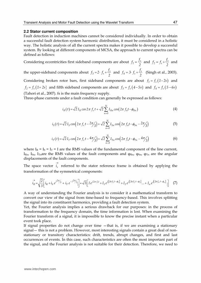
2.2 Stator current composition Fault detection in induction machines cannot be considered individually. In order to obtain a successful fault detection system harmonic distribution, it must be considered in a holistic way. The holistic analysis of all the current spectra makes it possible to develop a successful system. By looking at different components of MCSA, the approach to current spectra can be defined as follows:

Considering eccentricities first sideband components are about s1

ff

2= and s

2 s

ff f

2= + and

the upper-sideband components about s3 s

ff 2 f

2= ⋅ + and s

4 s

ff 3 f

2= ⋅ + (Singh et al., 2003).

Considering broken rotor bars, first sideband components are about ( )1 sf f 1 2s= − and

( )2 sf f 1 2s= + and fifth sideband components are about ( )3 sf f 4 5s= − and ( )4 sf f 5 6s= −

(Tahori et al., 2007). fs is the main frequency supply. Three-phase currents under a fault condition can generally be expressed as follows:

( ) ( )N

R R s Rn n Rnn 0

i t 2 I cos 2 f t 2 I cos 2 f tπ π φ=

= + −∑ (4)

( ) ( ) ( )N

S S s Sn n Snn 0

2 2i t 2 I cos 2 f t 2 I cos 2 f t3 3π ππ π φ

== − + − −∑ (5)

( ) ( ) ( )N

T T s Tn n Tnn 0

4 4i t 2 I cos 2 f t 2 I cos 2 f t3 3π ππ π φ

== − + − −∑ (6)

where IR = IS = IT = I are the RMS values of the fundamental component of the line current, IRn, ISn, ITnare the RMS values of the fault components and φRn, φSn, φTn are the angular displacements of the fault components.

The space vector si→

referred to the stator reference frame is obtained by applying the

transformation of the symmetrical components:

[ ] [ ] [ ]1 1 2 2 n ns2 2j j j 2 f t j 2 f t j 2 f tj2 f t3 3

R R S T 1 2 n

2i i i e i e 3 I e I e I e ... I e

3

π π π φ π φ π φπ→ − − − −⎡ ⎤ ⎡ ⎤= + + = + + +⎢ ⎥ ⎢ ⎥⎣ ⎦⎣ ⎦ (7)

A way of understanding the Fourier analysis is to consider it a mathematical transform to convert our view of the signal from time-based to frequency-based. This involves splitting the signal into its constituent harmonics, providing a fault detection system. Yet, the Fourier analysis implies a serious drawback for our purposes: in the process of transformation to the frequency domain, the time information is lost. When examining the Fourier transform of a signal, it is impossible to know the precise instant when a particular event took place. If signal properties do not change over time —that is, if we are examining a stationary signal— this is not a problem. However, most interesting signals contain a great deal of non-stationary or transitory characteristics: drift, trends, abrupt changes, and first and last occurrences of events. In this case, such characteristics are often the most important part of the signal, and the Fourier analysis is not suitable for their detection. Therefore, we need to

www.intechopen.com


48

apply another signal processing technique, such as the Wavelet transform, that can reveal aspects that a simple Fourier analysis misses.

2.3 Continuous wavelet transform (CWT) The Fourier analysis consists in breaking up a signal into sine waves with different frequencies. Similarly, a wavelet analysis is the breaking-up of a signal into shifted and scaled versions of the function called the ‘mother wavelet’. The continuous wavelet transform is the sum over time of the signal multiplied by scaled and shifted versions of the wavelet. This process produces wavelet coefficients that are a function of scale and position.

The integral wavelet transform of a function ( ) 2f t L∈ with respect to an analyzing wavelet

φ is defined as

( ) ( ) ( )b ,aW f b ,a f t t dtφ φ∞−∞= ∫ (8)

where

( )b ,a

t b1t a 0

aaφ φ −= > (9)

Parameters b and a are called translation and dilation parameters respectively. The

normalization factor a is included so that b ,aφ φ=

The expression for the inverse wavelet transform is

( ) ( ) ( )b ,a2

1 1f t db W f b ,a t da

C aφφ

φ∞ ∞−∞ −∞ ⎡ ⎤= ⎣ ⎦∫ ∫ (10)

Where Cφ is a constant that depends on the choice of wavelet and is given by

( ) 2

ˆC dφ

φ ω ωω= < ∞∫ (11)

The coefficients constitute the results of a regression of the original signal performed on the wavelets. A plot can be generated with the x-axis representing position along the signal (time), the y-axis representing scale, and the color at the x-y point representing the magnitude of wavelet coefficient C. These coefficient plots are generated with graphical tools.

2.4 Discrete wavelet transform (DWT) The discrete version of the wavelet transform, DWT, consists in sampling the scaling and shifted parameters, but neither the signal nor the transform. This leads to high-frequency resolution at low frequencies and high-time resolution for higher frequencies, with the same time and frequency resolution for all frequencies. A discrete signal x[n] can be decomposed as (Mallat, 1998):

www.intechopen.com


49

[ ] [ ] [ ]0 0

o

J 1

j ,k j ,k j ,k j ,kk j j k

x n a n d nφ ϕ−=

= +∑ ∑∑ (12)

where

[ ]nφ is the scaling function,

[ ] 00

0

jj2

j ,k n 2 (2 n k)φ φ= − , is the scaling function at a scale of ojs 2= shifted by k,

[ ]nϕ , is the mother wavelet,

[ ] ( )jj2

j ,k n 2 2 n kϕ ϕ= − , is the mother wavelet at a scale of js 2= shifted by k,

0j ,ka , is the approximation coefficients at a scale of ojs 2=

j ,kd , is the detail coefficients at a scale of ojs 2=

and JN 2= , where N is the number of x[n] samples. The scaling function can be defined as an aggregation of wavelets at scales larger than 1. A discrete signal can be constructed by using a sum of J-j0 details and an approximation to 1 of

a signal at a scale of ojs 2= . A quick way to obtain the forward DWT coefficients is to use the filter bank structure shown in Figure 3. The approximation coefficients at a lower level are transferred through a high-pass (h[n]) and a low-pass filter (g[n]), followed by a downsampling by two to compute both the detail (from the high-pass filter) and the approximation (from the low-pass filter) coefficients at a higher level. The two filters are linked to each other and they are known as quadrature mirror filters. High-pass and low-pass filters are derived from the mother wavelet and the scaling function, considered respectively in (Mallat, 1998) and (Mallat, 1989).

g[n]

h[n]

2

x[n2

g[n]

h[n]

2

2

g[n]

h[n]

2

2

Level 1 detail coefficients




Fig. 3. Wavelet tree decomposition for three levels of detail

The various frequency range coverings for the details and the final approximation for a three-level decomposition are shown in Figure 4. These are directly related to the bands where the analysis will be performed.

www.intechopen.com


50

Detail

Level 1Detail

Level 2DetailLevel 3

Approx.Level 3

fs/2fs/4fs/8fs/160

Fig. 4. Frequency ranges for details and final approximation

Figure 5 represents in a graphical manner the time-frequency window, which has better resolution on the time domain for high frequencies, and better frequency resolution for low frequencies, which means fewer resources for processing.

∧Δϕ1

2

a1a

ωω

∧Δϕ0

2

a

12aϕΔ

0a

ω

tab00

+tab11

+ t

Fig. 5. Time-Frequency window for the wavelet transform

The shape of the frequency response for these filters depends on the type and the order of the mother wavelet used in the analysis. In order to avoid overlapping between two adjacent frequency bands, a high-order mother wavelet has to be used that results in a high-order frequency filter. In order to separate the different frequency bands there is an obvious trade-off between the order of the mother wavelet and the computational cost. Thus, intensive study is needed in order to adapt the order of the mother wavelet to the requirements. Taking a common wavelet family such as the Daubechies mother wavelet, the mother wavelet time shape shows an evolution if we just change the Daubechies order as is shown in Figure 6. Yet, this does not provide clear information for our purpose.

www.intechopen.com


51

Fig. 6. Daubechies mother wavelet time evolution for order increase

Figure 7 shows the frequency response for low-pass and high-pass filters, which determines the detail and approximation decomposition for different orders. For low orders the power of one harmonic near the cut frequency could be split into two different details. This could give a false impression of the the time evolution of the analyzed signal's frequency component. By increasing the Daubechies order it is possible to idealize the filters and, hence, to obtain better frequency decomposition.

Fig. 7. Low- and high-pass filter frequency response corresponding to details

Figure 8 shows an example of this drawback. A test signal has been built with two harmonic components, one at 100 Hz and the other one at 45 Hz, and the signal has been sampled at 1000 Hz. The wavelet analysis is performed with a Daubechies db3 mother wavelet.

www.intechopen.com


52

Harmonic content due to the 100 Hz superimposed frequency appears on details 2 and 3; when it should only appear on detail 3, corresponding to the analysis band between 125 and 62.5 Hz. A high-order Daubechies mother wavelet is needed to prevent this drawback, which is due to the db3 associated filter not being ideal enough to filter the 100 Hz harmonic content on detail 2.

Fig. 8. Test decomposition signal with an overlapping effect

2.5 Power detail density (PDD) In a classical Fourier analysis, the power of a signal can be obtained by integrating the power spectral density (PSD), which is the square of the Fourier transform’s absolute value. The power carried by a defined spectral band can be obtained by integrating the PSD along this band. A similar derivation can be obtained for a wavelet transform. The power detail density (PDD) can be described as the squares of the coefficients for one particular detail. The power energy carried by this detail can be obtained by integrating its PDD. Discrete wavelet transforms show variations in the harmonic amplitude and location, and are the most suitable transform to be applied to non-stationary signals. The power detail density function resulting from a wavelet transform has proven to be one of the best suited methods for motor fault analysis under variable load, which presents the stator current as a non-stationary signal.

www.intechopen.com


53

The average power for a signal ( )x t is:

( ) ( )2 21 1P lim x t dt lim x t dt

2 2

ττττ ττ τ

∞− −∞→∞ →∞

⎡ ⎤ ⎡ ⎤= =⎢ ⎥ ⎢ ⎥⎣ ⎦⎣ ⎦∫ ∫ (13)

Applying Parseval’s theorem, this could be expressed as:

( ) ( ) ( )22 x1 1 1 1

P lim x d lim d S d2 2 2 2 2

τ ττττ τωω ω ω ω ωπ τ π τ π

∞ ∞− −∞ −∞→∞ →∞

⎡ ⎤⎡ ⎤ ⎢ ⎥= = =⎢ ⎥ ⎢ ⎥⎣ ⎦ ⎣ ⎦∫ ∫ ∫ (14)

Where:

( ) ( ) 2x

S lim2

ττ

ωω τ→∞⎡ ⎤⎢ ⎥= ⎢ ⎥⎣ ⎦

(15)

( )S ω is the spectral density of the signal ( )x t , and represents the distribution or the density of power as a function of ω . The energy of a discrete signal can be calculated by averaging the square of all the signal components inside the unity window, following equation 12:

( ) ( )( )T2

R

0

1Power i t t dt

Tφ= ∗∫ (16)

3. Experimental results

3.1 Experimental setup A three-phase, 1.1 kW, 380 V and 2.6 A, 50 Hz, 1410 rpm, four-pole induction motor was used in this study. Firstly, its healthy performance was analyzed and, afterwards, a sixth of the rotor bars was damaged as is shown in Figure 8. The motor nameplate is shown as follows:

Induction motor Value

Rated power 1.1kW. :Y 400/ D 230V

2.6/4.5A

Number of poles 4

Nominal speed 1410 rev/min

Cos ϕ 0.81

Table I. Specifications for an induction motor

The current has been measured by an A622 Tektronix 100 Ampere AC/DC current probe. The current ranges are 0/100 mV/A, and the typical DC accuracy is ±3% ± 50 mA at 100 mV/A (50 mA to a 10 A peak). The frequency range extends from DC to 100 kHz (-3 dB). The test rig and the data processing are displayed in Figure 9.

www.intechopen.com


54

Wavelet Details

Load Torque

Control

Fig. 9. Experimental setup

Load control has been implemented by using a PMSM and an inverter where variable load torque was introduced. The variable load torque follows an implemented increasing ramp as a torque control reference. Figure 10 depicts the evolution of the acquired currents.

12 12.5 13 13.5 14 14.5 15-5

-4

-3

-2

-1

0

1

2

3

4

5

Ia

Time (s)

Am

plit

ude

(A)

Fig. 10. Current supply to the motor

3.2 Signal acquisition requirements When carrying out experimental analyses one of the key elements to obtain good results is to choose appropriate acquisition parameters: sampling frequency and number of samples. There are three different constraints: analysis signal bandwidth, frequency resolution for the FFT analysis and wavelet decomposition spectral bands. For an IM, the most significant information about the stator current signal is focused around the 0-400 Hz band (Devaney et al., 2004), (Benbouzid et al., 2000) & (Thomson et al., 2003). The application of Nyquist’s theorem results in a minimum sampling frequency (fs) of 800 Hz.

www.intechopen.com


55

Furthermore, in case of an FFT analysis, it is necessary to get the right resolution. As for the inverter supply, several harmonics could be mixed up in case low resolution of the band side was chosen. The minimum resolution needed in order to obtain good results is 0.5 Hz. Equation (17) defines the number of samples to achieve the correct resolution required.

ss

fN

R= (17)

Ns is the number of samples needed and R is the resolution. On the other hand, wavelet analysis will show different frequency bands, centered at different frequencies. Frequency bands will depend on the sampling frequency, and will decrease as shown in Figure 4. The band covered by the wavelet decomposition will start with

,4 2sf f⎡ ⎤⎢ ⎥⎣ ⎦ and will then decrease as of 1

2 . The band suitable for analysis is about 40 Hz

(Tahori et al., 2007), needs to be covered by one detail, and depends on the sampling frequency. Finally, a sample frequency fs = 6 kHz was chosen and 50,000 samples were obtained. The full analysis band ranges from 0 to 3 kHz with a resolution of 0.12 Hz for the FFT analysis. The frequency bands of the wavelet decomposition are shown in Table II.

Decomposition details Frequency bands (Hz)

Detail at level 1 3000-1500 Detail at level 2 1500-750 Detail at level 3 750-375 Detail at level 4 375-187.5 Detail at level 5 187.5-92.75 Detail at level 6 92.75-46.37 Detail at level 7 46.37-23.18

Table II. Wavelet decomposition frequency bands for our test

3.3 Experimental results This section presents the experimental results. To clearly demonstrate the effectiveness of the method, different test have been performed. Firstly, tests were done in order to verify the state of the faulty motor at nominal torque on stationary state. These allow us to check MCSA harmonics resulting from the fault condition and their amplitude. The results show us that the performance of the DWT is far superior to the FFT. Finally, PSD calculations over the wavelet details are used to define a fault factor. After an FFT analysis, the current spectra for a faulty motor operating under constant and nominal load torque and a frequency supply of 50 Hz show a mark with an amplitude of 0.15 A (Figure 1) caused by a fault in the motor’s rotor bars. Equation (2) determines the frequency where the fault harmonics are located. The frequency of the fault harmonic depends on the slip, and the slip, in turn, depends on the load torque. This means that a variable load torque condition results in a time-dependent slip value, which causes variations in the spectrum. The measured speed values have a slip between 5 and 10%. Frequency locations for the fault harmonic are depicted in equations (18) and (19).

www.intechopen.com


56

( )fault s sf f 1 2 50(1 2 0.05) 45Hz= − = − ⋅ = (18)

( )fault s sf f 1 2 50(1 2 0.1) 40Hz= − = − ⋅ = (19)

Figure 11 corresponds to experimental harmonic distribution for a faulty motor working under variable load torque. An FFT analysis shows the spread of the power of a fault harmonic along the spectrum and the decrease of its amplitude. The wavelet analysis shows the temporary changes in the fault frequency band, and achieves great results under these particular conditions.

Fig. 11. Spectrum under variable load conditions

The harmonic amplitude found due to the fault (2.5 mA) is too low to use standard FFT. The wavelet transform will be used in order to find the correct amplitude. The CWT scalogram is shown in Figure 12. It clearly shows the fault evolution on the increased value from 30 to 50 coefficients

Fig. 12. Coefficient scalogram for the continuous wavelet transform

Figures 13 and 14 show the details of the wavelet decomposition for healthy and faulty motors when computing the transform with a Daubechies 23 mother wavelet. Daubechies 23 ensures correct signal decomposition, isolating the fault harmonic content, which gives proper results for our diagnostic purposes.

www.intechopen.com


57

Fig. 13. DWT decomposition of a healthy motor

Fig. 14. DWT decomposition of a faulty motor

www.intechopen.com


58

Detail levels of high frequency bands provide virtually no information about the original signal. Detail 6 corresponds to the frequency band of the main harmonic and detail 7 corresponds to the frequency band where the fault harmonic is located in the test. Comparing Figure 13 to Figure 14, we can clearly see the increase of the coefficient values as a result of the fault condition on the depicted scalograms (cfs). Also, the increase of the signal content is clearly appreciated on details 4, 5 and 7. Promising results are also obtained using wavelet transforms and evaluating the proper signal evolution during acquisition time. Figure 14 shows the advantage of the use of wavelets under variable load torque. Comparing the FFT decomposition and the DWT proves how using the Fourier decomposition (Figure 11) will reveal low amplitude for the spectrum in the 40 Hz band, lower than 3 mA. However, analyzing the wavelet time-amplitude decomposition (Figure 14) will show that the amplitude value follows the change of the amplitude in the fault harmonic over time, eventually achieving a value higher than 0.15 A when maximum torque is applied. The maximum torque value is the same that was applied to the constant torque test. The result of the analysis using the wavelet decomposition under a variable load torque matches the results obtained using an FFT analysis in the constant load torque test (Figure 1.) To perform the diagnosis, we also need to determine the fault factor, which is defined as the estimation of the energy content of any decomposed detail. Energy is estimated applying equation (16). Table III illustrates the energy increment for a fault condition of the approximation and detail decompositions at level 7. This energy has been calculated according to equation (12).

Power [W] D1 D2 D3 D5 D6 D7

Healthy motor Phase A 0.00 0.00 0.11 9.9 929.2 35.75

Motor with broken rotor bars Phase A 0.00 0.00 1.1 13 887.7 88.11

Table III. Power spectral density (power detail density)

Table III clearly illustrates the energy increment of the decompositions chosen. Both wavelet decompositions shown in Table III can be used to detect rotor faults in the motor at any point of operation. The fault condition can be clearly identified by analyzing the energy content of faulty harmonics (PSD). A clear efficiency decrease of about 6% is appreciated on the main supply harmonic and a clear increase due to the fault condition is appreciated on the fault frequency bands. In D7, which is placed over the main fault harmonic, there is an increase of 2.5 times the energy content. This technique combines the time and frequency analysis of wavelet decompositions, allowing for better fault factor estimation. Combining DWT and PSD allows for further development of expert algorithms to implement an autonomous fault diagnosis system for induction machines.

4. Conclusions

This chapter has introduced the problems of fault detection under a variable load torque. The classical computation of MCSA using the FFT introduces average errors in the

www.intechopen.com


59

amplitude harmonic evaluation, hampering fault detection. To ensure proper results a time-frequency analysis is required. As with time-frequency analysis, the proposed alternative is the discrete wavelet transform (DWT). DWT has different resolutions on time and frequency depending on the different frequency bands defined. The use of DWT ensures good time-frequency analysis. DWT has been used to analyze motors with eccentricity and broken rotor bars under fault conditions, achieving good results. Moving toward an autonomous diagnosis sensor, a fault condition parameter has been studied and the power spectral density has been used as a power detail density with wavelets, ensuring proper results. To sum up, we can say that: • Wavelet decomposition is the proper technique for isolating time components of non-

stationary signals, with low computational costs. • Analyzing the energy of some wavelet decompositions is the right way to detect rotor

faults in industrial motor applications with non-constant load torque. • The evolution of wavelet coefficients gives good results in terms of fault detection. • Orthogonal properties of wavelet functions ensure the detection of major variations on

small amplitude signals, which is the case of reduced fault condition operation.

5. References

B. Ayhan, M.Y.Chow, H.J. Trussell, M.H. Song, E.S. Kang, H.J.Woe: “Statistical Analysis on a Case Study of Load Effect on PSD Technique for Induction Motor Broken Rotor Bar Fault Detection”, Symposium on Diagnostics for Electric Machines, Power

Electronics and Drives, SDEMPED 2003, Atlanta GA, USA 24-26 August 2003. Khmais Bacha, Humberto Henao, Moncef Gossa, Gérard-André Capolino; “Induction

machine fault detection using stray flux EMF measurement and neural network-based decision”; Electric Power Systems Research, Volume 78, Issue 7, July 2008, Pages 1247-1255.

Mohamed El Hachemi Benbouzid: “A Review of Induction Motor Signature Analysis as a Medium for Faults Detection”, IEEE Transactions on Industrial Electronics, Vol. 47, nº 5, Oct 2000, pp. 984-993.

Hakan Çalış and Abdülkadir Çakır, Rotor bar fault diagnosis in three phase induction motors by monitoring fluctuations of motor current zero crossing instants; Electric

Power Systems Research, Volume 77, Issues 5-6, April 2007, Pages 385-392. J. R. Cameron, W. T. Thomson, and A.. B. Dow: “Vibration and current monitoring for

detecting airgap eccentricity in large induction motors”, IEE Proceedings, pp. 155-163, Vol.133, Pt. B, No.3, May 1986.

W. Deleroi, “Broken bars in squirrel cage rotor of an induction motor- Part 1: Description by superimposed fault currents” (in German) Arch. Elektrotech, vol. 67, pp. 91-99, 1984.

Michael J. Devaney, Levent Eren; “Detecting Motor Bearing Faults” IEEE Transactions on

Instrumentation and Measurement Magazine, pp 30-50, December 2004. Andrew K.S. Jardine, Daming Lin, Dragan Banjevic, A review on machinery diagnostics and

prognostics implementing condition-based maintenance, Mechanical Systems and

Signal Processing 20 (2006), 1483-1510

www.intechopen.com


60

Chinmaya Kar, A.R. Mohanty, Monitoring gear vibrations through motor current signature analysis and wavelet transform, Mechanical Systems and Signal Processing 20 (2006) 158-187.

S. G. Mallat “A Theory for multiresolution Signal Decomposition: The Wavelet Representation” IEEE Transactions on Pattern Analysis and Machine intelligence Vol II No 7, July 1989.

S. G. Mallat, “A Wavelet tour of signal Processing” Academic Press 1998 Second Edition Dick Meador; “Tools for O&M, from Building Controls to Thermal Imaging” O&M Workshop

for Government Facility Managers, June 19, 2003, US Department of Energy. Gang Niu, Achmad Widodo, Jong-Duk Son, Bo-Suk Yang, Don-Ha Hwang, Dong-Sik Kang;

“Decision-level fusion based on wavelet decomposition for induction motor fault diagnosis using transient current signal”; Expert Systems with Applications, Volume 35, Issue 3, October 2008, Pages 918-928.

G. K. Singh, Saad Ahmed Saleh Al Kazzaz; “Induction machine drive condition monitoring and diagnostic research—a survey”, Electric Power Systems Research, Volume 64, Issue 2, February 2003, Pages 145-158.

Easa Tahori Oskouel, Alan James Roddis: “A condition Monitoring Device using Acoustic Emission Sensors and data Storage Devices”, UK Patent Application GB 2340034 A, data of publication 03/14/2007.

W. T. Thomson, and M. Fenger: “Case histories of current signature analysis to detect faults in induction motor drives”, IEEE International Conference on Electric Machines and

Drives, IEMDC'03, Vol. 3, pp. 1459-1465, June 2003. Abhisek Ukil and Rastko Živanović, “Abrupt change detection in power system fault

analysis using adaptive whitening filter and wavelet transform”; Electric Power

Systems Research, Volume 76, Issues 9-10, June 2006, Pages 815-823 Simi P. Valsan, K.S. Swarup; “Wavelet based transformer protection using high frequency

power directional signals”; Electric Power Systems Research, Volume 78, Issue 4, April 2008, Pages 547-558.

www.intechopen.com

Discrete Wavelet Transforms - Theory and ApplicationsEdited by Dr. Juuso T. Olkkonen

ISBN 978-953-307-185-5Hard cover, 256 pagesPublisher InTechPublished online 04, April, 2011Published in print edition April, 2011

InTech EuropeUniversity Campus STeP Ri Slavka Krautzeka 83/A 51000 Rijeka, Croatia Phone: +385 (51) 770 447 Fax: +385 (51) 686 166www.intechopen.com

InTech ChinaUnit 405, Office Block, Hotel Equatorial Shanghai No.65, Yan An Road (West), Shanghai, 200040, China

Phone: +86-21-62489820 Fax: +86-21-62489821

Discrete wavelet transform (DWT) algorithms have become standard tools for discrete-time signal and imageprocessing in several areas in research and industry. As DWT provides both frequency and locationinformation of the analyzed signal, it is constantly used to solve and treat more and more advanced problems.The present book: Discrete Wavelet Transforms: Theory and Applications describes the latest progress inDWT analysis in non-stationary signal processing, multi-scale image enhancement as well as in biomedicaland industrial applications. Each book chapter is a separate entity providing examples both the theory andapplications. The book comprises of tutorial and advanced material. It is intended to be a reference text forgraduate students and researchers to obtain in-depth knowledge in specific applications.

How to referenceIn order to correctly reference this scholarly work, feel free to copy and paste the following:

Jordi Cusidó i Roura and Jose Luis Romeral Martínez (2011). Transient Analysis and Motor Fault Detectionusing the Wavelet Transform, Discrete Wavelet Transforms - Theory and Applications, Dr. Juuso T. Olkkonen(Ed.), ISBN: 978-953-307-185-5, InTech, Available from: http://www.intechopen.com/books/discrete-wavelet-transforms-theory-and-applications/transient-analysis-and-motor-fault-detection-using-the-wavelet-transform

© 2011 The Author(s). Licensee IntechOpen. This chapter is distributedunder the terms of the Creative Commons Attribution-NonCommercial-ShareAlike-3.0 License, which permits use, distribution and reproduction fornon-commercial purposes, provided the original is properly cited andderivative works building on this content are distributed under the samelicense.

https://creativecommons.org/licenses/by-nc-sa/3.0/

transient analysis and motor fault detection using …...transient analysis and motor fault...

Documents