Tactical Missiles

Autopilot Design

Aerodynamic Control

— D Viswanath

Acknowledgment

I am most grateful to my Dr. S. E. Talole, for introducing me to this subject. His

teachings have been my source of motivation throughout this work.

(D Viswanath)

Apr 2011

1

Synopsis

Broadly speaking autopilots either control the motion in the pitch and yaw planes, in

which they are called lateral autopilots, or they control the motion about the fore and

aft axis in which case they are called roll autopilots. Lateral ”g” autopilots are designed

to enable a missile to achieve a high and consistent ”g” response to a command. They

are particularly relevant to SAMs and AAMs. There are normally two lateral autopilots,

one to control the pitch or up-down motion and another to control the yaw or left-right

motion.

The requirements of a good lateral autopilot are very nearly the same for command

and homing systems but it is more helpful initially to consider those associated with

command systems where guidance receiver produces signals proportional to the mis-

alignment of the missile from the line of sight (LOS).

The effectiveness of a guided missile weapon system, in terms of accuracy and prob-

ability of kill, depends greatly on the response characteristics of the complete guidance,

control, and airframe loop. Since the accuracy or effectiveness of a guided missile de-

pends greatly on the dynamics of the missile, particularly during the terminal phase of

its flight, it is often desirable to predict its flight dynamics in the early preliminary-design

phase to assure that a reasonably satisfactory missile configuration is realized.

The missile control methods can be broadly classified under aerodynamic control and

thrust vector control. Aerodynamic control can be further classified into Cartesian and

polar control methods while thrust vector control can be further classified under gim-

baled motors, flexible nozzles (ball and socket), interference methods (spoilers/vanes),

secondary fluid or gas injection and vernier engines (external or extra engines). Aero-

dynamic control methods are generally used for tactical missiles.

2

Contents

Acknowledgment 1

Synopsis 2

Contents 3

1 Modeling Roll, Pitch and Yaw Dynamics Using Aerodynamic Deriva-

tives 1

1.1 Introduction . . . . . . . . . . . . . . . . . . . . . . . . . . . . . . . . . . 1

1.2 Translational and Rotational Dynamics of Missile Autopilot . . . . . . . 1

1.2.1 Dynamics of Yaw Autopilot . . . . . . . . . . . . . . . . . . . . . 2

1.2.2 Dynamics of Pitch Autopilot . . . . . . . . . . . . . . . . . . . . . 2

1.2.3 Dynamics of Roll Autopilot . . . . . . . . . . . . . . . . . . . . . 2

1.3 Roll Dynamics using Aerodynamic Derivatives . . . . . . . . . . . . . . . 2

1.3.1 Normalized Form . . . . . . . . . . . . . . . . . . . . . . . . . . . 3

1.3.2 Example[1] . . . . . . . . . . . . . . . . . . . . . . . . . . . . . . 4

1.3.3 Transfer Function Model of a Missile : Roll Dynamics . . . . . . . 4

1.4 Yaw Dynamics using Aerodynamic Derivatives . . . . . . . . . . . . . . . 5

1.4.1 Transfer Function Model of a Missile : Yaw Dynamics . . . . . . . 7

3

1.4.2 Latax of the missile due to Rudder Deflection . . . . . . . . . . . 8

1.5 Pitch Dynamics using Aerodynamic Derivatives . . . . . . . . . . . . . . 9

1.5.1 Transfer Function Model of a Missile : Pitch Dynamics . . . . . . 9

1.5.2 Transfer functions for Angle of Attack and Latax of the missile

due to Elevator Deflection . . . . . . . . . . . . . . . . . . . . . . 9

References 10

4

Chapter 1

Modeling Roll, Pitch and Yaw

Dynamics Using Aerodynamic

Derivatives

1.1 Introduction

Aerodynamic derivatives are devices enabling control engineers to obtain transfer

functions defining the response of a missile to aileron, elevator or rudder inputs. With

the roll, pitch and yaw dynamics under consideration, aerodynamic derivatives are force

derivatives if they are used in force equation and moment derivatives if they are used in

moment equation.

1.2 Translational and Rotational Dynamics of Mis-

sile Autopilot

The final simplified equations for forces and moments acting on the missile which rep-

resent the translational and rotational dynamics of the missile respectively were derived

in Chapter 2 as follows: -

1

1.2.1 Dynamics of Yaw Autopilot

It can be seen that the equations

Y = m(dv

dt+ rU) (1.1)

N = rIz

are coupled and produce moments about z axis or torque about z axis or the yaw

movement and are used for design of yaw autopilot.

1.2.2 Dynamics of Pitch Autopilot

Similarly the eqns

Z = m(dw

dt− qU) (1.2)

M = qIy

are for pitching dynamics and are used for design of pitch autopilot.

1.2.3 Dynamics of Roll Autopilot

The roll autopilot dynamics is represented by the equation

L = pIx (1.3)

1.3 Roll Dynamics using Aerodynamic Derivatives

The roll dynamics can be rewritten as given below:-

pIx = L (1.4)

where p is the angular velocity about the x-axis; Ix is the moment of inertia about the

x-axis and L is the total rolling moment acting on the missile.

2

The total rolling moment L is a function of the angular velocity p and the aileron

deflection ξ, i.e.,

L = L(p, ξ) (1.5)

Hence using partial derivatives, the roll dynamics can be expressed as follows:-

pIx =∂L

∂ξξ +

∂L

∂pp (1.6)

The partial derivatives ∂L∂ξ

and ∂L∂p

are also known as the aerodynamic moment derivatives

and represented by Lξ and Lp respectively. In other words, Lξ is the roll moment

derivative due to aileron deflection ξ and Lp is the roll moment derivative due to angular

velocity p. Thus

pIx = Lξξ + Lpp (1.7)

Note:- Lξ is not a linear function of ξ due to two reasons:-

(i) Aileron effectiveness decreases with total incidence θ.

(ii) For a given θ, Lξ is not a linear function of ξ, although the graph passes through

origin.

However, bearing in mind that in most applications ξ is unlikely to exceed a few degrees

we can consider Lξ as constant.

1.3.1 Normalized Form

The normalised form of roll dynamics using aerodynamic dervatives can be expressed

considering the moment of inertia Ix(or A) to be constant as follows:-

pIx = Lξξ + Lpp (1.8)

p =LξIxξ +

LpIxp

p = lξξ + lpp

where lξ and lp are the normalised roll moment derivatives.

Sign Convention for Roll Moments Positive aileron deflection results in the sign

of moments being negative. Hence Lξ and Lp are negative values.

3

1.3.2 Example[1]

Consider an air to air homing missile whose roll moment of inertia is A = 0.96Kgm2

and is assumed to fly at a constant height of 1500m. The table 1.1 shows that the roll

derivatives, aerodynamic gains and time constants vary largely due to the variability in

the launch speeds in the range of M = 1.4 to M = 2.8.

Various quantities M = 1.4 M = 1.6 M = 1.8 M = 2.0 M = 2.4 M = 2.8

−Lξ 7050 8140 9100 10200 11700 13500

−Lp 22.3 24.9 27.5 30.3 34.5 37.3

Ta =−ALp

0.043 0.0385 0.0349 0.0316 0.0278 0.0257

LξLp

316 327 331 336 340 362

Table 1.1: Roll Derivatives, Gains and Time Constants

1.3.3 Transfer Function Model of a Missile : Roll Dynamics

Thus the above equation of roll dynamics where aerodynamic derivatives have been

used can now be easily expressed in transfer function form where the input is the aileron

deflection (ξ) and output is the roll rate (p).

Using Laplace Transforms

p = lξξ + lpp (1.9)

sp(s) = lξξ(s) + lpp(s)

(s− lp)p(s) = lξξ(s)

p(s)

ξ(s)=

lξ(s− lp)

4

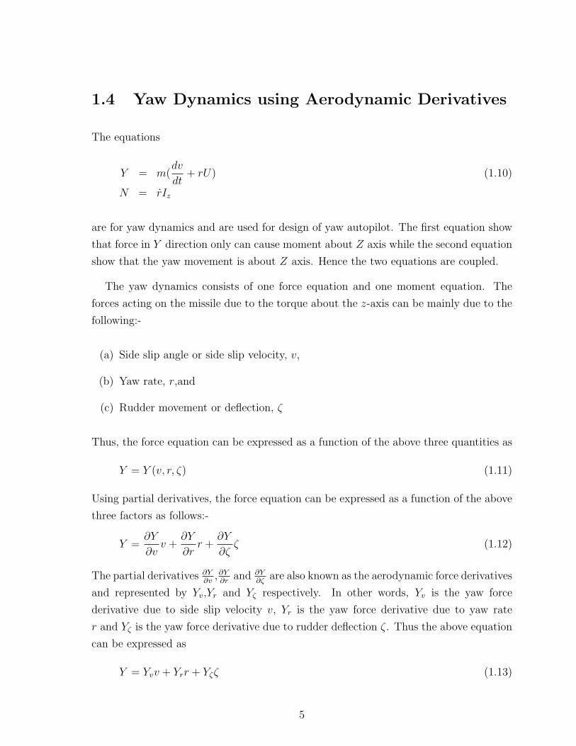
1.4 Yaw Dynamics using Aerodynamic Derivatives

The equations

Y = m(dv

dt+ rU) (1.10)

N = rIz

are for yaw dynamics and are used for design of yaw autopilot. The first equation show

that force in Y direction only can cause moment about Z axis while the second equation

show that the yaw movement is about Z axis. Hence the two equations are coupled.

The yaw dynamics consists of one force equation and one moment equation. The

forces acting on the missile due to the torque about the z-axis can be mainly due to the

following:-

(a) Side slip angle or side slip velocity, v,

(b) Yaw rate, r,and

(c) Rudder movement or deflection, ζ

Thus, the force equation can be expressed as a function of the above three quantities as

Y = Y (v, r, ζ) (1.11)

Using partial derivatives, the force equation can be expressed as a function of the above

three factors as follows:-

Y =∂Y

∂vv +

∂Y

∂rr +

∂Y

∂ζζ (1.12)

The partial derivatives ∂Y∂v

,∂Y∂r

and ∂Y∂ζ

are also known as the aerodynamic force derivatives

and represented by Yv,Yr and Yζ respectively. In other words, Yv is the yaw force

derivative due to side slip velocity v, Yr is the yaw force derivative due to yaw rate

r and Yζ is the yaw force derivative due to rudder deflection ζ. Thus the above equation

can be expressed as

Y = Yvv + Yrr + Yζζ (1.13)

5

Re-writing the force equation in yaw,

Y = m(dv

dt+ rU) (1.14)

m(dv

dt+ rU) = Yvv + Yrr + Yζζ

dv

dt+ rU =

Yvmv +

Yrmr +

Yζmζ

dv

dt=

Yvmv +

Yrmr +

Yζmζ − rU

dv

dt= yvv + yrr + yζζ − rU

v = yvv + (yr − U)r + yζζ

where yv, yr and yζ are the normalized aerodynamic force derivatives in yaw.

Similarly, the moment N is also a function of the side slip velocity v, yaw rate r and

rudder deflection ζ and can be expressed as

N = N(v, r, ζ) (1.15)

Using partial derivatives, the moment about Z axis can be expressed as

N =∂N

∂vv +

∂N

∂rr +

∂N

∂ζζ (1.16)

The partial derivatives ∂N∂v

,∂N∂r

and ∂N∂ζ

are also known as the aerodynamic moment

derivatives in yaw and represented by Nv,Nr and Nζ respectively. In other words, Nv is

the yaw moment derivative due to side slip velocity v, Nr is the yaw moment derivative

due to yaw rate r and Nζ is the yaw moment derivative due to rudder deflection ζ. Thus

the above equation can be expressed as

N = Nvv +Nrr +Nζζ (1.17)

Re-writing the moment equation in yaw,

N = rIz (1.18)

rIz = Nvv +Nrr +Nζζ

r =Nv

Izv +

Nr

Izr +

Nζ

Izζ

r = nvv + nrr + nζζ

where nv, nr and nζ are the normalized aerodynamic moment derivatives in yaw.

6

1.4.1 Transfer Function Model of a Missile : Yaw Dynamics

The yaw dynamics using aerodynamic force and moment derivatives was derived in the

above subsection and the final equations for forces and moments in the yaw plane were

expressed in the form of a set of simultaneous equations as follows:-

v = yvv + (yr − U)r + yζζ (1.19)

r = nvv + nrr + nζζ

Transfer function is defined as the ratio of the Laplace Transform of the output

variable to the Laplace Transform of the input variable. Here the control model is

the missile under test and input is deflection, say, rudder while output is either lateral

acceleration in Y direction or velocity component in Y direction (side slip angle in steady

state) or yaw rate in Y direction.

Taking Laplace Transforms of the two equations given above gives

sv(s) = yvv(s) + (yr − U)r(s) + yζζ(s) (1.20)

sr(s) = nvv(s) + nrr(s) + nζζ(s)

Simplifying the above equation gives

(s− yv)v(s)− (yr − U)r(s) = yζζ(s) (1.21)

−nvv(s) + (s− nr)r(s) = nζζ(s)

Expressing the above equations using matrices gives[(s− yv) −(yr − U)

−nv (s− nr)

] [v(s)

r(s)

]=

[yζ

nζ

]ζ(s) (1.22)

Solving the above equations using Cramer’s rule gives two transfer functions where

the input is the rudder deflection, ζ(s) and the two outputs are v(s) and r(s) which are

7

given as follows:-

v(s)

ζ(s)=

det

[yζ −(yr − U)

nζ (s− nr)

]

det

[(s− yv) −(yr − U)

−nv (s− nr)

] (1.23)

v(s)

ζ(s)=

yζ(s− nr) + nζ(yr − U)

s2 − (yv + nr) + yv nr − nv(yr − U)

and

r(s)

ζ(s)=

det

[(s− yv) yζ

−nv nζ

]

det

[(s− yv) −(yr − U)

−nv (s− nr)

] (1.24)

r(s)

ζ(s)=

nζ(s− yv) + nvyζs2 − (yv + nr) + yv nr − nv(yr − U)

The equation v(s)ζ(s)

describes how side slip velocity or angle acts on the missile while

the equation r(s)ζ(s)

describes how yaw rate acts on the missile.

1.4.2 Latax of the missile due to Rudder Deflection

The force equation in yaw plane was initially derived as follows:-

m(v + rU) = Y (1.25)

Force is the product of mass and acceleration, i.e.,in other words

m(v + rU) = may (1.26)

where ay is the lateral acceleration in yaw plane. Thus, taking Laplace transform of

above equation and simplifying gives

ay(s) = s v(s) + U r(s) (1.27)

8

Dividing the above equation throughout by ζ(s) gives the transfer function for lateral

acceleration in yaw plane due to rudder deflection as follows:-

ay(s)

ζ(s)= s

v(s)

ζ(s)+ U

r(s)

ζ(s)(1.28)

Substituting the right hand side of equations for v(s)ζ(s)

and r(s)ζ(s)

in the above equation gives

ay(s)

ζ(s)= s

yζ(s− nr) + nζ(yr − U)

s2 − (yv + nr) + yv nr − nv(yr − U)+U

nζ(s− yv) + nvyζs2 − (yv + nr) + yv nr − nv(yr − U)

(1.29)

Simplifying the above equation gives

ay(s)

ζ(s)=s2yζ − snryζ + snζyr − U(nζyv − nvyζ)

s2 − (yv + nr) + yv nr − nv(yr − U)(1.30)

This is an important equation which is used in the design of lateral autopilot.

1.5 Pitch Dynamics using Aerodynamic Derivatives

The equations for the pitching dynamics of the missile are given by

Z = m(dw

dt− qU) (1.31)

M = qIy

1.5.1 Transfer Function Model of a Missile : Pitch Dynamics

Using the steps used in the derivation for various transfer functions of the missile model

in the yaw plane, analogous transfer functions for the missile model in pitch plane also

can be derived as follows.

1.5.2 Transfer functions for Angle of Attack and Latax of the

missile due to Elevator Deflection

9

References

[1] P. Garnell, Guided Weapon Control Systems. London: Brassey’s Defence Publishers,

1980.

10